Implications from the velocity profile of the M87 jet: a possibility of a slowly rotating black hole magnetosphere

Abstract

Motivated by the measured velocity profile of the M87 jet using the KVN and VERA Array (KaVA) by Park et al. (2019b) indicating that the starting position of the jet acceleration is farther from the central engine of the jet than predicted in general relativistic magnetohydrodynamic simulations, we explore how to mitigate the apparent discrepancy between the simulations and the KaVA observation. We use a semi-analytic jet model proposed by Tomimatsu & Takahashi (2003) consistently solving the trans-magnetic field structure but neglecting any dissipation effects. By comparing the jet model with the observed M87 jet velocity profile, we find that the model can reproduce the logarithmic feature of the velocity profile, and can fit the observed data when choosing $c/(100r_{g})\lesssim\Omega_{F}\lesssim c/(70r_{g})$ where $r_{g}$ is the gravitational radius. While a total specific energy (${\cal E}$) of the jet changes the terminal bulk Lorentz factor of the jet, a slower angular velocity of the black hole magnetosphere (funnel region) ($\Omega_{F}$) makes a light-cylinder radius ($r_{\rm lc}$) larger and it consequently pushes out a location of a starting point of the jet acceleration. Using the estimated $\Omega_{F}$ we further estimate the magnetic field strength on the event horizon scale in M87 by assuming Blandford-Znajek (BZ) process is in action. The corresponding magnetic flux threading the event horizon of M87 is in good agreement with a magnetically arrested disc (MAD) regime.

1 Introduction

The formation mechanism of relativistic jets in active galactic nuclei (AGNs) remains elusive a longstanding problem in astrophysics. Towards better understanding of this longstanding issue, significant forward steps have been made by recent VLBI observations of the notable nearby radio galaxy M87. The radio galaxy M87 is the one of the closest examples of the radio jet and it provides us the best opportunity to explore the jet launching mechanism at its base (e.g., Junor et al., 1999; Hada et al., 2011; Abramowski et al., 2012; Hada et al., 2014; Kim et al., 2018; Walker et al., 2018). Recently, the Event Horizon Telescope (EHT) has delivered the first resolved images of M87*, the supermassive black hole in the center of the M87 galaxy. From the EHT data, the $D=16.8\pm 0.8$ Mpc and $M_{\bullet}=(6.5\pm 0.7)\times 10^{9}M_{\odot}$ are derived and the corresponding angular radius of the gravitational radius $\theta_{g}={GM_{\bullet}/Dc^{2}}=3.8\pm 0.4~{}{\mu}$as where $G$ and $c$ are the gravitational constant, and the light speed, respectively (Event Horizon Telescope Collaboration, 2019a, b, c, d, e, f). The gravitational radius is given by $r_{\rm g}\equiv GM_{\bullet}/c^{2}$ and this corresponds to the relation of $1~{}{\rm mas}=263~{}r_{g}$.

Based on mm/sub-mm VLBI observations, the jet base of M87 has been indicated to be magnetic-energy dominated based on the energetics at the optically thick region against synchrotron self-absorption (SSA) process (Kino et al., 2014, 2015b). Now it is widely considered that magnetic field plays an important role in the formation of the relativistic jet (e.g., Blandford et al., 2019). At the footpoint region of the jet, a scenario in which the jet formation is caused by the extraction of the black hole’s rotational energy via the large scale magnetic field that penetrates the black hole event horizon, has been proposed by Blandford & Znajek (1977) (hereafter BZ77), which is so-called BZ process. Although this BZ process looks promising so far, there are still many details of the physical process that are not yet understood. Given this background, we will discuss a jet model driven by a large-scale magnetic field in this work.

Toward a better understanding of the jet formation, the $z$-dependence of the jet velocity ($u_{p}$) where the subscript $p$ denotes the poloidal velocity is one of the fundamental quantities to be explored. The profile of $u_{p}$ in M87 has been intensively investigated via VLBI monitoring for years (Kovalev et al., 2007; Asada et al., 2014; Mertens et al., 2016; Hada et al., 2016, 2017; Walker et al., 2018). Recently, further comprehensive dedicated observation of densely-sampled monitoring at 22 and 43 GHz in 2016 using the KVN and VERA (KaVA) array, (as a sub-array of the East Asian VLBI Network (Wajima et al., 2016; Asada et al., 2017; An et al., 2018, and references therein)) was performed as one of the large programs of KaVA array(Niinuma et al., 2014; Kino et al., 2015a) and it particularly clarified the velocity field on 0.3-10 mas scale by Park et al. (2019b). Interestingly, Park et al. (2019b) pointed out that the measured velocity profile is not described as a single streamline but rather explained by multiple ones, and the location where the jet starts acceleration is farther from the central engine than expected in GRMHD simulations. The existence of such a discrepancy has been also pointed out in recent literature (Nakamura et al., 2018; Chatterjee et al., 2019).

The goal of this work is to find a possible solution to mitigate the apparent discrepancy between the theoretical model of magnetically accelerated jet and the observed velocity field profile in the M87 jet by Park et al. (2019b). It is important to note a possibility that blob motions observed by VLBI may be caused by apparent changes of dissipative non-steady pattern structures such as shocks, turbulence and local instabilities (e.g., Cohen et al., 2014; Mertens et al., 2016) that can be different from the fluid velocity itself. The purpose of this paper is not to deny this possibility. However, it is difficult to ascribe all the moving blob motions to dissipative pattern structures, which do not reflect actual fluid motions since the one-side feature ubiquitously seen in radio jets in AGNs is essentially explained by the Doppler boosting effect due to actual fluid motions. Therefore, while recognizing the possibility that some of the observed velocities could be partially mixed with pattern velocities, we will investigate the nature of the stationary jet in this paper.

In § 3, we briefly overview the model proposed by Tomimatsu & Takahashi (2003) (hereafter TT03). In § 4, we show basic properties of $u_{p}$ based on TT03 model. In § 5, we apply TT03 model to the M87 jet and we constrain on ${\cal E}$ and $\Omega_{F}$ of M87 by comparing the model predicted $u_{p}$ to the VLBI measured $u_{p}$. In § 6, we make comparisons between our result and previous works, and then discuss implications of our result. In § 7, we summarize the present work. In this work, we use the natural unit ($c=1$, $G=1$), otherwise stated.

2 Overall setting

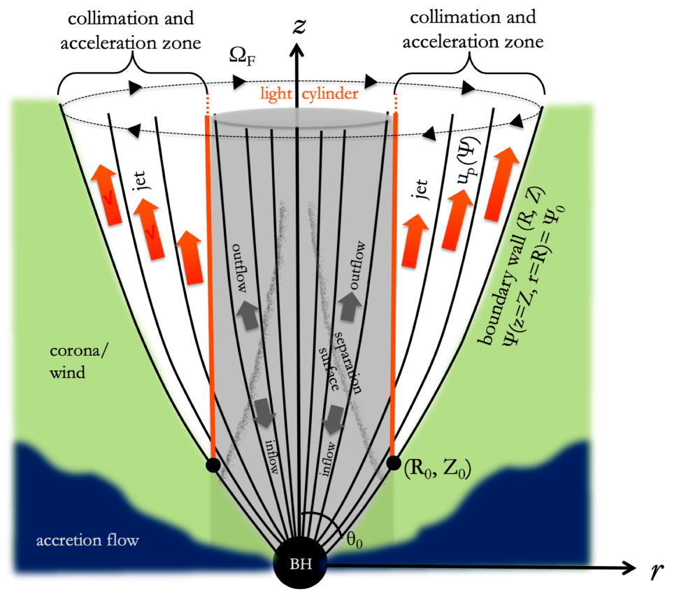
Figure 1: A schematic illustration of Poynting flux dominated jet confined by the outer boundary wall made of corona/wind region. The jet is accelerated outside the light cylinder and that is denoted as acceleration region (collimation and acceleration zone). In the highly magnetized funnel region, a stagnation surface is generated that separates the inflow and outflow regions. TT03 appropriately describes the poloidal velocity field of the jet flow in the outer region of the light cylinder (equivalent to the outer light surface) denoted as $u_{p}(\Psi)$. The angular velocity of the magnetic field lines is denoted as $\Omega_{F}$. TT03 model does not describe the interior of the light cylinder. We use cylindrical coordinates. The position coordinates of the outer boundary wall is denoted by the capital letters ($R$, $Z$). The value of the $z$ coordinate of the light surface is different for each magnetic field line. The position where each magnetic field line intersects the light surface is the position of the light cylinder for each magnetic field line, thus the more distant the light surface for the inner magnetic field line, the farther away it is. We denote the $z$ coordinate where the boundary wall (equivalent to the outermost magnetic field line) intersects the light surface as $(R_{0},Z_{0})$.

Before going into a detailed description of the model, it would be useful to describe the overall setting and the core motivation of the present work. Figure 1 summarizes the overall picture of the situation considered here. In this work, we utilize the MHD model proposed by TT03 in the framework of special relativity (i.e., SRMHD). It shows a schematic illustration of Poynting flux dominated jet confined by the outer boundary wall made of corona/wind region. In the black hole magnetosphere, due to the balance between the gravitational force of the black hole and magneto-centrifugal force, a stagnation (also known as separation) surface is generated that separates the inflow and outflow regions (e.g., Takahashi et al., 1990; McKinney, 2006; Pu et al., 2015; Pu & Takahashi, 2020). For clarity, in Figure 1, we show the region where we will apply TT03 model. Comparing semi-analytical approaches and GRMHD simulation approaches, it is known that the semi-analytical approaches have the following advantages. The large spatial extent of the acceleration region has posed a challenge for such calculations by GRMHD simulations and they tend to be eventually limited by computational costs and numerical dissipation (e.g., McKinney, 2006; Komissarov et al., 2007, for details), while semi-analytic approaches are free from these concerns. When discussing properties of axisymmetric and steady MHD flows in general, the magnetic field geometry should be consistent with Grad-Shafranov (GS) equation, and the flow should be trans-fast-magnetosonic. However, it is technically difficult to obtain a solution satisfying both of these conditions (e.g., Beskin, 2010, for review). TT03 model is the only semi-analytic solution to satisfy both of these conditions. Since $u_{p}$ profile is sensitive to the magnetic field geometry, we use TT03 model in this work.

TT03 model is prescribed by two model parameters, i.e., total energy (${\cal E}$) and the angular velocity of magnetic field lines $\Omega_{F}$ for a given streamline of the flow. Therefore, our main goal in this work can be rephrased as constraining ${\cal E}$ and $\Omega_{F}$ by matching $u_{p}$ profiles by KaVA observation and TT03 model. It would be worth stressing in advance that the physical quantity $\Omega_{F}$ is one of the most important quantities in BZ process. The BZ process is a magnetic extraction of the spin energy of a Kerr black hole within the force-free limit and it is thought to be a plausible production mechanism for the relativistic jets in AGNs. BZ77 showed that a frame-dragging effect of the central Kerr black hole can induce an outward flux of electromagnetic energy along magnetic field lines threading the event horizon, at the expense of the black hole’s rotational energy and its expected power ($L_{BZ}$) is given by

$$L_{BZ}\propto\Omega_{F}(\Omega_{H}-\Omega_{F})B_{H}^{2},$$ (1)

where $B_{H}$ is the magnetic field strength threading the event horizon. GRMHD simulations of jet productions indicate that powerful jets can be produced by BZ process, when an angular velocity of the central Kerr BH ($\Omega_{H}$) is not too small (e.g., Zamaninasab et al., 2014, and references therein) and higher spin of the black holes for powerful outflows is also in good agreement with the indications from the observational data (e.g., Sikora et al., 2007). One of the questions to be addressed in this paper will be whether the M87 jet meets the condition of the activation of the BZ process, i.e., $0<\Omega_{F}<\Omega_{H}$ or not. If the condition seems to hold in M87, then we will estimate $B_{H}$ by using the estimated $\Omega_{F}$.

3 Model

We briefly overview the work of TT03. Hereafter, the cylindrical coordinate $(t,r,\phi,z)$ is used and the corresponding line element is given by $ds^{2}=c^{2}dt^{2}-dr^{2}-dz^{2}-r^{2}d\phi^{2}$.

3.1 Basic Assumptions

The basic assumptions in TT03 are as follows.

• A cold (zero pressure), steady ($\partial/\partial t=0$), axisymmetric ($\partial/\partial\phi=0$) special relativistic MHD jet flow is assumed.

• Effects of general relativity (GR) are not included and a Minkowski space-time is assumed in this work. The assumption is well justified on the spatial scale dealt with in the present work. A formulation including GR effects (but assuming the magnetic field geometry) is presented in Takahashi & Tomimatsu (2008); Pu & Takahashi (2020); Huang et al. (2020).

• Any dissipation and energy loss processes are not included in TT03 model. Dissipation effects caused by various instabilities are generally considered to become more pronounced as the jet moves downstream (e.g., Chatterjee et al., 2019, and references therein).

With these assumptions, the flow is characterized by five physical quantities, i.e., the poloidal and toroidal velocity ($u_{p}$ and $u_{\phi}$) and the poloidal- and toroidal magnetic field ($B_{p}$ and $B_{\phi}$), and the plasma mass density $\rho$ Poloidal magnetic field and 4-velocity of the fluid are given by $B_{p}^{2}=B_{z}B^{z}+B_{r}B^{r}$ and $u_{p}^{2}=u_{z}u^{z}+u_{r}u^{r}$, respectively. With the Lorentz factor of the poloidal velocity $\Gamma=\sqrt{1+u_{p}^{2}}$, $u_{p}=\Gamma v_{p}$ hold where $v_{p}$ is the 3-velocity of the poloidal velocity (Tomimatsu, 1994).

3.2 Field aligned conserved quantities

Here we introduce the well known magnetic-field aligned conserved quantities (i.e., ${\cal E}$, ${\cal L}$, $\Omega_{F}$, and $\eta$, see later), which facilitates understanding flow dynamics. The $B_{p}$ and $u_{p}$ will be determined by GS equation and the relativistic Bernoulli equation together with appropriate conditions (such as boundary condition, trans-magnetosonic condition). The remaining three quantities will be given by conservation laws and boundary conditions at the plasma source. The toroidal components $u_{\phi}$ and $B_{\phi}$ are obtained by the $B_{p}$ and $u_{p}$ and the conserved quantities.

Using the vector potential of the magnetic field ($\vec{A}$), the magnetic field is given by $\vec{B}=\nabla\times\vec{A}$. A stationary and axisymmetric ideal MHD flow provides the existence of a magnetic flux (stream) function ($\Psi(r,z)$). The toroidal component of $\vec{A}$ plays a role in the magnetic flux (stream) function and it is written as

$$\Psi(r,z)=A_{\phi}$$ (2)

(e.g., Blandford & Znajek, 1977). The magnetic fields are structured along the surface of $\Psi(r,z)=$constant. The poloidal magnetic field is given by $\vec{B}_{p}=\frac{\nabla\Psi(r,z)\times\vec{e}_{\phi}}{2\pi r}$ where $\vec{e}_{\phi}$ is the $\phi$-component unit vector, which can be written as $B^{r}=-\frac{1}{r}\frac{\partial\Psi(r,z)}{\partial z}$, and $B^{z}=\frac{1}{r}\frac{\partial[\Psi(r,z)]}{\partial r}$.

For a stationary, axisymmetric MHD flow, there are four conserved quantities along a constant $\Psi$ surface, which are $\eta(\Psi)$, ${\cal E}(\Psi)$, ${\cal L}(\Psi)$, and $\Omega_{F}(\Psi)$, are the particle flux, the total specific energy the total specific angular-momentum, and the angular velocity of a magnetic field line, respectively (Camenzind, 1986, and references therein). The total specific energy and angular-momentum can be decomposed into two terms as follows.

$${\cal E} = {\cal E}_{\rm EM}+{\cal E}_{\rm MA},\quad{\cal E}_{\rm EM}=-\frac{r\Omega_{F}B_{\phi}}{4\pi\eta},\quad{\cal E}_{\rm MA}=\Gamma,$$ (3)

$${\cal L}={\cal L}_{\rm EM}+{\cal L}_{\rm MA},\quad{\cal L}_{\rm EM}=-\frac{rB_{\phi}}{4\pi\eta},\quad{\cal L}_{\rm MA}=\Gamma r^{2}\Omega,$$ (4)

where $\Omega$ is the angular velocity of the plasma in the jet and the relation $\eta=\rho u_{p}/B_{p}$ holds. The $\sigma$ parameter describing a degree of magnetization is given by

$$\sigma=\frac{{\cal E}_{\rm EM}}{{\cal E}_{\rm MA}}.$$ (5)

The total specific energy and angular momentum are decomposed into the electro-magnetic and matter (plasma) part and the corresponding subscripts are EM and MA, respectively. We add to note that $\eta$ and ${\cal E}$ reflect the amount of mass-loading/particle-injection into the jet (e.g., Mościbrodzka et al., 2011; Levinson & Rieger, 2011; Toma & Takahara, 2012; Hirotani & Pu, 2016; Hirotani, 2018; Chen et al., 2018; Levinson & Cerutti, 2018; Parfrey et al., 2019; Kisaka et al., 2020) although detailed studies on particle-injection is beyond the scope of this paper.

The relativistic Alfvén Mach number is defined as

$$M^{2}\equiv\frac{4\pi\rho u_{p}^{2}}{B_{p}^{2}}.$$ (6)

The behavior of $M^{2}$ at the fast magnetosonic point is the key to understanding the jet acceleration in the framework of MHD model.

3.3 Relativistic Bernoulli equation

Here we briefly review of relativistic Bernoulli equation. The equation is also known as a poloidal wind equation. Following the framework of TT03, the normalized $r$ by the light-cylinder radius ($r_{\rm lc}$) is introduced as

$$\hat{r}\equiv\frac{r}{r_{\rm lc}}=r\Omega_{F},\quad\Omega_{F}(\Psi)=const.$$ (7)

In this work, we focus on the region where $\hat{r}>1$ holds. If a poloidal velocity reaches the relativistic fast-magnetosonic wave speed at a certain point, then the term $\partial M^{2}/\partial r$ may diverge at the point. Such a flow solution is unphysical. For a physical trans-fast magnetosonic flow solution, it is necessary to satisfy the critical condition there. To remove this technical difficulty to find a special class of solutions of $M^{2}$ which satisfies this critical condition, TT03 introduced a regular function of

$$\xi(\hat{r})\equiv\frac{E_{p}}{|B_{\phi}|}\equiv\hat{r}\frac{B_{p}}{|B_{\phi}|}$$ (8)

where $E_{p}$ is the poloidal component of the electric field. The $\xi$ is set as a smooth function of $\hat{r}$ including the fast magnetosonic point along each given $\Psi=$constant surface. It is worth stressing that $\hat{r}$ dependence on $\xi$, to be determined by the GS equation, governs the magnetic field geometry and the corresponding velocity profile.

The Bernoulli equation is given by

$$(1+u_{p}^{2})(M^{2}+\hat{r}^{2}-1)^{2} =$$

$${\cal E}_{\rm co}^{2}(1-2M^{2}-\hat{r}^{2}) + \left({\cal E}^{2}-\frac{{\cal L}^{2}\Omega_{F}^{2}}{\hat{r}^{2}}\right)M^{4}$$ (9)

where the total specific energy measured in the co-rotation frame (${\cal E}_{\rm co}$) with the frame’s rotation speed of $\Omega_{F}$ is defined as

$${\cal E}_{\rm co} \equiv {\cal E}-{\cal L}\Omega_{F}.$$ (10)

By using the $\xi$, the Bernoulli equation reduces to the quadratic equation for $M^{2}$

$${\cal A}M^{4}-2{\cal B}M^{2}+{\cal C}=0$$ (11)

where the coefficients ${\cal A}$, ${\cal B}$, and ${\cal C}$ are functions of $\Omega_{F}$, ${\cal E}$, $\xi^{2}$, and $\hat{r}^{2})$. Readers can refer to TT03 for details. Next, we consider Mach numbers at Alfven radius and fast magnetosonic radius. One can define the Alfven radius normalized by $r_{\rm lc}$ and the Alfven Mach number at the Alfven radius as

$$M_{A} \equiv \frac{{\cal E}-{\cal L}\Omega_{F}}{{\cal E}}=1-\hat{r}_{A}^{2},\quad\hat{r}_{A}\equiv\frac{{\cal L}\Omega_{F}}{{\cal E}}<1,$$ (12)

which means the Alfven radius is within the light cylinder. Similarly, at the fast magnetosomic point ($\hat{r}=\hat{r}_{F}$),

$$M_{F}^{2}\equiv\frac{(1-\xi^{2})\hat{r}^{2}+\xi^{2}}{\xi^{2}}$$ (13)

Thus, the behavior of the flow is controlled by the pitch angle of the magnetic field, which is reflected in $\xi$. For instance, $\xi$ smaller than the critical value leads to $M^{2}=\infty$ at finite $r$.

3.4 The approximated GS equation

The approximated GS equation derived by TT03 (Eqs. (39) and (42) in TT03), which is valid for highly relativistic outflow of $1\leq{\cal E}_{\rm co}\ll{\cal E}$, is given by

$$\frac{1}{\Psi_{r}}\frac{\partial}{\partial r}\left[\frac{\xi^{2}\eta^{2}}{1+(\Psi_{z}/\Psi_{r})^{2}}\left({\cal E}-\frac{{\cal L}\Omega_{F}}{\hat{r}^{2}}\right)\right]\simeq$$

$$(1+\hat{M}^{2})\Omega_{F}^{2}\frac{\partial}{\partial\Psi}\left(\frac{\eta^{2}}{\Omega_{F}^{2}\hat{M}^{4}}\right).$$ (14)

where $\partial\Psi(r,z)/\partial r=\Psi_{r}$ and $\partial\Psi(r,z)/\partial z=\Psi_{z}$. Since collimated jets in AGNs are discussed in the present work, the collimated geometry of the magnetic field is assumed as follows:

$$\frac{\Psi_{z}}{\Psi_{r}}<\frac{1}{{\cal E}}\ll 1.$$ (15)

Then one can obtain the general solution of an analytical form for the approximated GS equation (Eqs. (51) and (54) in TT03) described as

$$\frac{2(\hat{r}/{\cal E})^{2}(\hat{M}^{2}+1)}{\hat{M}^{2}+2(\hat{r}/{\cal E})^{2}}=\ln\left[\frac{2(\hat{r}/{\cal E})^{2}}{\hat{M}^{2}}+1\right].$$ (16)

From this, we can numerically obtain $\hat{M}(\hat{r})$. By numerically solving the below shown equation (Eqs. (52) and (55) in TT03), one can obtain $\Psi(\hat{r},\hat{z})$

$$\frac{\Psi}{\Psi_{0}}\left[\frac{1}{\hat{M}^{2}(\hat{r}/{\cal E})}+\frac{1}{2(\hat{r}/{\cal E})^{2}}\right]=\frac{1}{\hat{M}^{2}(\theta_{0}\hat{z})}+\frac{1}{2(\theta_{0}\hat{z})^{2}},$$ (17)

where $\hat{z}\equiv z\Omega_{F}/\cal{E}$ and $\theta_{0}$ is the half opening angle of the jet (see the next section). It is well known that the geometry of magnetic field line is essential for jet acceleration and thus solving $\Psi$ is essential for discussing the velocity field. Qualitatively, magnetic field lines which bend towards the rotation axis realize a location of $r_{F}$ at a finite distance from the central engine (e.g., Begelman & Li, 1994; Takahashi & Shibata, 1998).

3.5 Outer boundary wall condition

The outer boundary wall condition would be given by a parabolic streamline along the poloidal magnetic field lines. Since there are multiple normalization, it would be useful to explicitly write down the boundary condition here. The outer boundary wall shape denoted as ($Z$, $R$) in the cylindrical coordinate and it satisfies the following relation:

$$\frac{Z}{r_{\rm lc}{\cal E}}\theta_{0} = \left(\frac{R}{r_{\rm lc}{\cal E}}\right)^{q}(1\leq q\leq 2),$$ (18)

where the $\theta_{0}$ is the half-opening angle of the jet at the inlet boundary and the magnetic flux function on the boundary wall satisfies $\Psi(z=Z,r=R)=\Psi_{0}$. Note that the case of $q=1$ corresponds to a conical boundary wall shape. In this work, we will give the value of $a$ with reference to the overall results of the detailed VLBI observations in §4.

4 Basic properties of the velocity profile

By solving these Bernoulli and GS equations, one can obtain a consistent $z$-dependence of $u_{p}$. Before applying TT03 model to the M87 jet, here we overview the basic properties of $u_{p}$. In § 4.1, we show the $z$-profiles of $u_{p}$ for multi-streamlines with different $\Psi$. In § 4.2, we present ${\cal E}$ and $\Omega_{F}$ dependence of the $u_{p}$ profile which will be important for comparisons of TT03 model with the observed $u_{p}$ of the M87 jet.

4.1 $\Psi$ dependence

Figure 2 shows the $z$-profile of $u_{p}$ for each streamline. First, we briefly review the $r$-profile of $u_{p}$ for a given single $\Psi$=const. streamline. One can define the square of the normalized relativistic Alfven Mach number $\hat{M}^{2}(\Psi)\equiv\frac{M^{2}(\Psi)}{\hat{r}^{2}}=\frac{1}{\sigma(\Psi)}$. It is also convenient to rewrite $\Gamma$ (equivalent to $u_{p}$) as

$$\Gamma={\cal E}-\frac{u_{p}}{\xi\hat{M}^{2}}.$$ (19)

This shows $z$-dependence of jet acceleration by the energy conversion. From Eq. (16), in the inner zone $(1\ll\hat{r}\ll{\cal E})$, one can obtain

$$\hat{M}^{2}\approx\hat{r}/{\cal E},\quad(1\ll\hat{r}\ll{\cal E})$$ (20)

This initial phase is identical to the linear acceleration phase indicated by Tchekhovskoy et al. (2008). In the asymptotic far zone ($\hat{r}\gg{\cal E}$), the acceleration profile gets deviated from the linear acceleration and it becomes a logarithmic accelerated phase as

$$\hat{M}^{2}\approx\ln\left(\frac{2\hat{r}^{2}}{({\cal E}\hat{M})^{2}}\right),\quad(\hat{r}\gg{\cal E}),$$ (21)

the emergence of the logarithmic acceleration phase after the linear acceleration phase is not only shown by TT03 but also pointed out in Beskin et al. (1998); Lyubarsky (2009). The transition from linear to logarithmic acceleration is caused by plasma inertia.

As for $\Psi$-dependence, faster $u_{p}$ is seen for larger $\Psi$ in Figure 2. This behavior is explained by a differential bunching of $B_{p}$ in the jet. As already known in previous works of GRMHD simulations (e.g., McKinney, 2006; Nakamura et al., 2018; Chatterjee et al., 2019), the energy conversion from ${\cal E}_{\rm EM}$ to ${\cal E}_{\rm MA}$ gets on at outer part of the jet flow with larger $\Psi$. Therefore, the faster $u_{p}$ is realized for larger $\Psi$.

4.2 ${\cal E}$ and $\Omega_{F}$ dependence

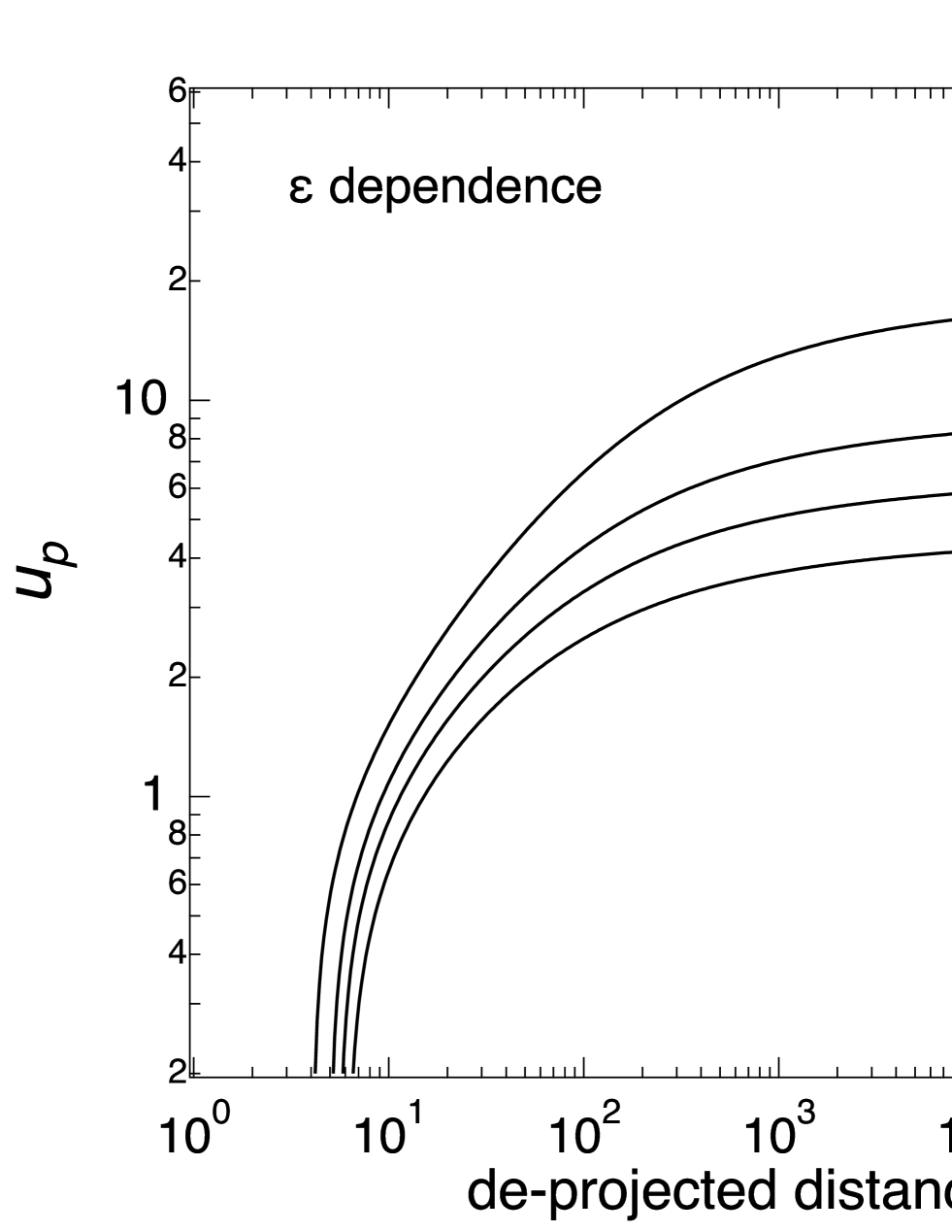
Figure 3: We show the ${\cal E}$ dependence of $u_{p}$.

In Figure 3, we show the ${\cal E}$-dependence of $u_{p}$. Here we demonstrate the cases with ${\cal E}=$5, 7, 10 and 20. In order to demonstrate the ${\cal E}$-dependence , we select the flow with $\Psi=\Psi_{0}$ for each ${\cal E}$ case. Since TT03 model does not include any energy dissipation processes, it is clear that the Lorentz factor asymptotically goes to the maximum value and it is given by

$${\cal E}=\Gamma_{\rm max}\quad(z\to\infty).$$ (22)

Since TT03 model describes an ideal magneto-transonic flow, the complete energy conversion from ${\cal E}_{\rm EM}$ to ${\cal E}_{\rm MA}$ realizes at infinity.

In Figure 4, we show the $\Omega_{F}$-dependence of $u_{p}$. Same as Figure 3, we select the flow with $\Psi=\Psi_{0}$ for each $\Omega_{F}$ case to present the $\Omega_{F}$-dependence. On the contrary to the case of varying ${\cal E}$, $\Omega_{F}$ does not alter the profile of $u_{p}$ itself. As already shown, $\Omega_{F}$ is governed by the light cylinder radius $r_{\rm lc}$ and it is given by $\Omega_{F}=1/r_{\rm lc}$. Slower rotation of $\Omega_{F}^{-1}$ leads to more distant starting point of the jet acceleration from the central BH.

4.3 Location of intersection between Boundary-wall and light-cylinder

In this work, a location of intersection between the boundary-wall ($\Psi=\Psi_{0}=1$ surface) and the light-cylinder is important. Hereafter, we denote the location as ($R_{0}$, $Z_{0}$). By inserting $R_{0}=r_{\rm lc}$ at Eq. (18), the location of $Z_{0}$, from which the jet acceleration starts (see Figure 1), is obtained as follows:

$$Z_{0}=100~{}r_{g}\left(\frac{\theta_{0}}{0.1}\right)^{-1}\left(\frac{r_{\rm lc}}{10r_{g}}\right){\cal E}^{1-q},$$ (23)

where it will turn out to be ${\cal E}^{1-q}\approx 0.2-0.5$ from observational properties of the M87 jet shown in the next section. We note that the geometrical factor $\theta_{0}$ also affects the location of $Z_{0}$.

5 Application to the M87 jet

Here we apply TT03 model to the $u_{p}$ measured in the M87 jet. The two parameters to be determined are ${\cal E}$, and $\Omega_{F}$. While ${\cal E}$ is easily constrained from the maximum speed of the M87 jet around HST-1 region, $\Omega_{F}$ has been poorly constrained by any observational data so far.

5.1 Maximum Lorentz factor

As mentioned, in the asymptotic zone ${\cal E}$ satisfies ${\cal E}\approx\Gamma_{\rm max}$. Regarding the maximum Lorentz factor, it is chosen to match with the HST-1 component at the $4\times 10^{5}~{}r_{s}$ (Biretta et al., 1999; Giroletti et al., 2012) and we set

$${\cal E}=10.$$ (24)

To clear up the essential discussion in this work, hereafter we fix the value ${\cal E}=10$ for simplicity, which never affects the main result of this work.

The jet half-opening angle is directly constrained by VLBI observations (Junor et al., 1999; Hada et al., 2016). Here, we set

$$\theta_{0}\approx 0.34~{}\tan^{-1}\left[\sin\left(\frac{\theta_{\rm view}}{17^{\circ}}\right)\tan\left(\frac{\theta_{0,\rm obs}}{50^{\circ}}\right)\right]~{}{\rm rad}$$ (25)

in our subsequent numerical calculations. The chosen value of the observed $\theta_{0,obs}$ is adopted from the result of the high dynamic range VLBA+GBT obseravation at 86 GHz, which indicate the $\sim 100^{\circ}$ of the full-opening angle at the jet base (Hada et al., 2016). The viewing angle of the M87 jet $\theta_{\rm view}$ has uncertainty and here we adopt the normalization of $17^{\circ}$ based on (Event Horizon Telescope Collaboration, 2019e).

5.2 Boundary-wall shape

In the present work, we identify the jet width profile measurement conducted by Asada & Nakamura (2012); Hada et al. (2013) as the boundary-wall shape. It means that the observed M87 jet is identical to the funnel region, in which the ordered magnetic field collimates and accelerates the plasma jet. It is, however, difficult to know exactly which magnetic field lines among the ordered fields are identical to the observationally measured jet profile. If no dissipation occurs at the boundary between the jet and surrounding matter and the funnel region is filled with radio emitting non-thermal electrons, then the outermost magnetic field lines on $\Psi=\Psi_{0}$ surface that thread the black hole are basically identical to the jet width profile measured by VLBI described above. In more realistic cases, however, the boundary region between a jet and a surrounding matter may become dissipative by reflecting the details of physical conditions at the boundary layer (e.g., Levinson & Globus, 2016; Chatterjee et al., 2019). It is also uncertain about where and how nonthermal electrons are produced and cooled down in the jet. Thus, model predicted images generally depend on assumptions in treatments of non-thermal electrons (e.g., Dexter et al., 2012; Takahashi et al., 2018; Event Horizon Telescope Collaboration, 2019e). Therefore, taking those uncertainties into account, we include all the allowed range of $q$ obtained by Asada & Nakamura (2012); Hada et al. (2013) is as follows:

$$1.3\lesssim q\lesssim 1.7.$$ (26)

In addition, TT03 model can describe the magnetic field bending around the characteristic distance $z_{\rm brk}$ where ${\cal E}_{\rm EM}\sim{\cal E}_{\rm MA}$ holds. It is obtained by the condition of $\hat{r}\approx{\cal E}$ at $R=R_{\rm brk}$ and given by $z_{\rm brk}=1000~{}r_{g}\left(\frac{{\cal E}}{10}\right)\left(\frac{\theta_{0}}{0.1}\right)^{-1}\left(\frac{r_{\rm lc}}{10~{}r_{g}}\right)$ in the deprojected distance (see eq. (56) in TT03).

5.3 Velocity profile

Here, we fit the observed $u_{p}$ data with the one predicted by TT03 model. At first, we explain how to do the fitting. As already mentioned, we fix ${\cal E}=10$ throughout this work. Therefore, the remaining model parameters to be adjusted are $\Omega_{F}$ (equivalent to $r_{\rm lc}$) and $\theta_{0}$. To properly search for the best fit $\Omega_{F}$ and $\theta_{0}$ taking the uncertainty into account, we impose the following condition.

1. From the currently measured range of $u_{p}$ (Park et al., 2019b, and references therein), we set the allowed range of $Z_{0}$ as $2\times 10^{2}~{}r_{g}\lesssim Z_{0}\lesssim 4\times 10^{2}~{}r_{g}$ in this work.

2. Based on VLBI observations, we set the allowed range of $\theta_{0}$ as $0.1\leq\theta_{0}\leq 0.34$ where the upper bound is given by Eq. (25) while the lower bound is assumed as $\theta_{0}=1/{\cal E}=0.1$.

3. The light-cylinder radius should be smaller than the jet radius in the jet acceleration region (i.e., $z\gtrsim Z_{0}$) within the framework of TT03 model. The jet width $R_{0}$ at $z\approx Z_{0}$ is measured as $R_{0}\approx 100~{}r_{g}$ (Hada et al., 2013).

4. As shown in Figure 4, $\Omega_{F}$ tightly links to $Z_{0}$. We will search for a best fit $\Omega_{F}$ so that the model predicted $u_{p}$ of the outer edge of the jet flow ($\Psi=\Psi_{0}$) does not largely exceed the observed data.

5. Taking various uncertainties into account, here we will perform the fitting for both $q=1.3$ and $q=1.7$ boundary-wall conditions and we will determine the allowed range of $\Omega_{F}$ in between those two best-fit values.

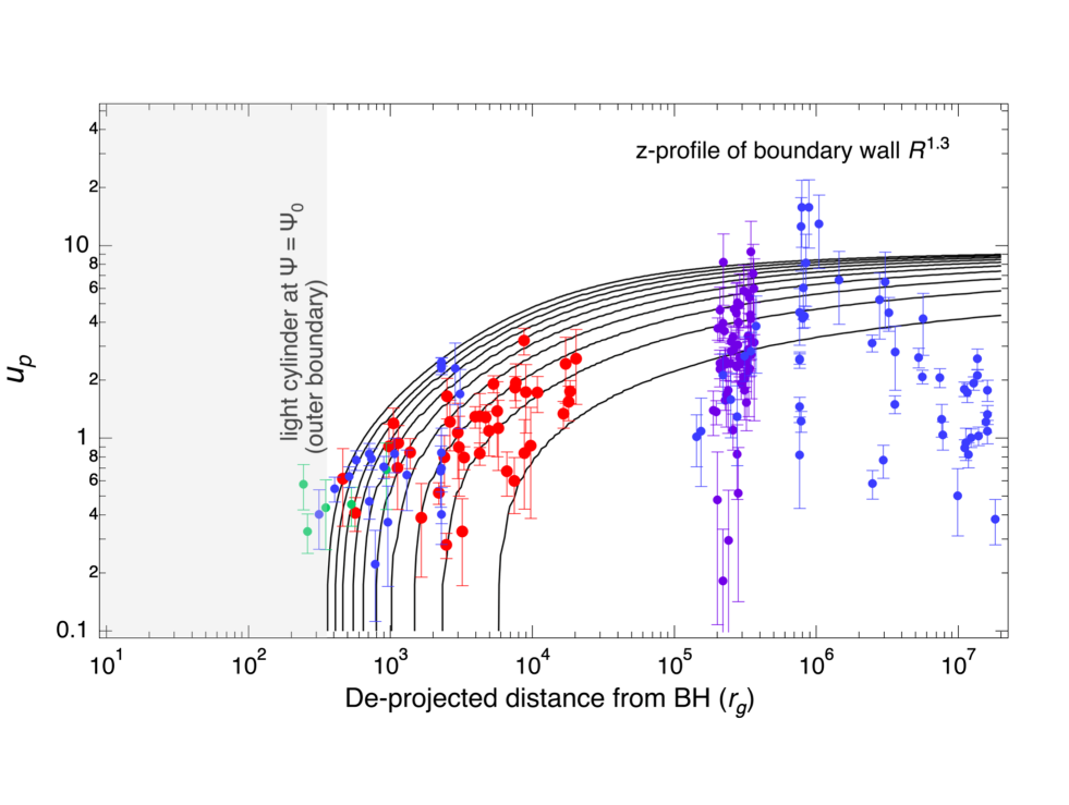
Figure 5: The comparison of the model predicted $u_{p}$ and and the VLBI measured $u_{p}$ as a function of deprojected distance $z$ from the black hole in unit of $r_{g}$. The observation data points are adopted from (Park et al., 2019b). The case in which the parameter $q=1.3$ is chosen for the boundary wall shape is presented here. Whereas TT03 model well reproduces the overall logarithmic acceleration of $u_{p}$, some offset remains at the inner region $z\lesssim 500~{}r_{g}$. We also note that it is natural for the observed data and the model to have a gap below $10^{6}~{}r_{g}$ since the region is beyond the domain of application of the model, where various dissipation processes are supposed to occur.

In Figure 5, we show the best fit profile of the $u_{\rm p}$ for the case of the boundary-wall with $q=1.3$. Same as Figure 2, we have plotted the multiple flow paths along with $\Psi=0.1\Psi_{0},0.2\Psi_{0},\dots,\Psi_{0}$. As shown in Figure 1, the jet flow is not heterogeneous but described as multiple laminar flow paths along multiple magnetic surfaces. The jet plasma is not essentially accelerated inside the light cylinder. That is because the plasma is co-rotating with the magnetic field lines inside the light cylinder. When the plasma exceeds the light cylinder radius, it cannot co-rotate with the magnetic field lines anymore and flows outward, and is accelerated in the poloidal direction. The KaVA observational data shown in Park et al. (2019b) indicates that the M87 jet logarithmically accelerates up to the HST1 scale. Hence the linear acceleration (e.g., Tchekhovskoy et al., 2008) is not able to explain the observed $u_{\rm p}$ profile. On the contrary, TT03 model predicts the logarithmic acceleration, which naturally agrees with the observed logarithmic $u_{\rm p}$ profile. As pointed out by Park et al. (2019b), the observed trend of the jet acceleration in M87 is slower than those indicated in GRMHD simulation in the literature and does not match each other. From Figure 5, one can find that our model can overcome this problem and explain with this observed velocity profile above $10^{3}~{}r_{g}$ scale. The reason is the best fit parameter $r_{\rm lc}\approx 70~{}r_{g}$ is larger than a typical one in GRMHD simulations. For instance, GRMHD simulation of the M87 jet in McKinney (2006) obtained $r_{\rm lc}\approx 10~{}r_{g}$. We thus find that the larger $r_{\rm lc}$ shifts the starting point of the jet acceleration, i.e., $Z_{0}$ and it can explain the observed $u_{p}$. The obtained distance is $Z_{0}\approx 3\times 10^{2}~{}r_{g}$. We add to note that the condition 3 holds only when $\theta_{0}\approx 0.1$. Hence we use this value although this is a factor of $\sim 3$ smaller than the $\theta_{0}$ indicated by 86GHz observation. An investigation of this mismatch is beyond the scope of this work since TT03 model cannot discuss anything inside the light cylinder.

In Figure 5, one can see that the innermost data points within $30~{}r_{g}$ do not match the model prediction. But it is not fatal. Although the detailed investigation is beyond the scope of this paper, this mismatch may suggest the need for effects not incorporated in TT03 model. In Takahashi et al. (2021), we discussed that differences in the angular momentum values of the plasma are one possibility to mitigate the discrepancy.

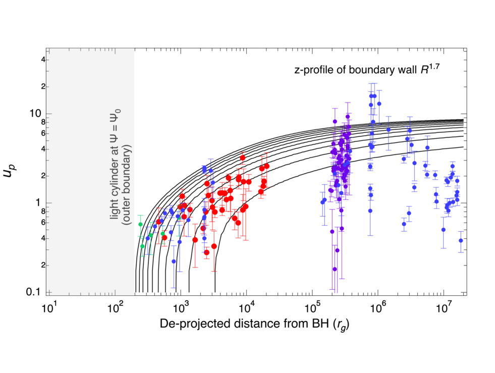
Figure 6: Same as Figure 2 but with $q=1.7$.

In Figure 6, we show the best fit profile of the $u_{\rm p}$ for the case of the boundary-wall with $q=1.7$. The overall behavior of the the model predicted $u_{p}$ profile is similar with the case with $q=1.3$. The difference between $q=1.3$ and $q=1.7$ cases is that the case with $q=1.7$ have a smaller (more gradual) slope of acceleration than the case with $q=1.3$. The best fit value adopted in Figure 6 is $r_{\rm lc}\approx 100~{}r_{g}$ and correspondingly we have $Z_{0}\approx 2\times 10^{2}~{}r_{g}$ in Figure 6.

Finally, by setting the result for the case of $q=1.3$ as the upper limit of $\Omega_{F}$ and setting the result with $q=1.7$ as the lower limit of $\Omega_{F}$, we obtain the allowed range of $\Omega_{F}$ as follows:

$$\frac{c}{100~{}r_{g}}\lesssim\Omega_{F}\lesssim\frac{c}{70~{}r_{g}}.$$ (27)

Thus, we find that the slower $\Omega_{F}$ compared to typical values in GRMHD simulations mitigates the velocity mismatch problem in the M87 jet pointed out in Park et al. (2019b).

5.4 $\sigma$ profile

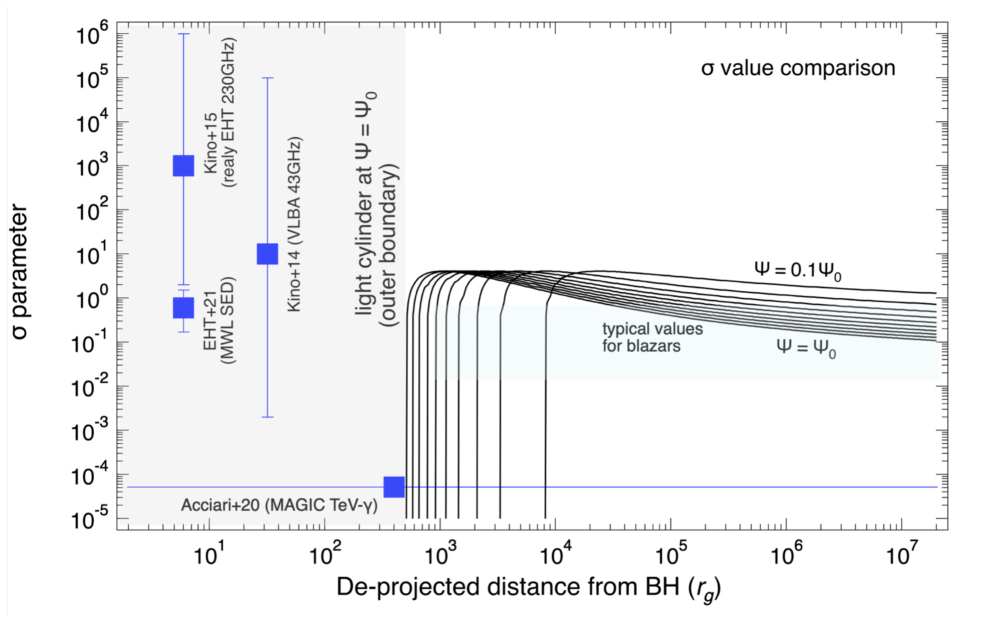
Figure 7: The comparison of the obtained $\sigma$ profile for each magnetic field lines and the estimations of the magnetization degrees constrained in previous literature for the M87 jet. For comparison, a region indicating typical values for the location and the magnetization degree of blazars is also shown by a light blue filled square. Unfortunately, the estimates made by Kino et al. (2014, 2015b) are in a region beyond the applicability of TT03 model (i.e., inside the light cylinder), which means that they cannot be directly compared with the obtained $\sigma$ curves presented here. The result reported by MAGIC Collaboration et al. (2020) indicates apparently much smaller magnetization degree than the values found in other reports.

In Figure 7, we show the corresponding $\sigma$ profile with $q=1.3$ together with the $\sigma$ values obtained in literatures. In general, there is a limitation for constraining a magnetization degree at a jet base from spectral energy distribution (SED) fitting of multi-wavelengths (MWL) data since collected flux data do not share a common single emission region due to different angular resolution of various telescopes. To overcome the limitation of MWL SED fitting, Kino et al. (2014) and Kino et al. (2015b) explore the energetics at the M87 jet base based on VLBI data alone together with the well-established process of synchrotron self-absorption (SSA). In Figure 7, we include these values in the literatures by setting $\sigma={\cal E}_{\rm EM}/{\cal E}_{\rm MA}\approx U_{B}/U_{\pm}$. Unfortunately, sub-mm radio-emitting 40 $\mu$as region in (Kino et al., 2014, 2015b; EHT MWL Science Working Group et al., 2021) is within the light cylinder, which is not described by TT03. Therefore, it is not possible to directly compare the obtained $\sigma$ profile with the constrained $\sigma$ those previous works. At least, what one can conservatively say is that a high value of $\sigma$ inside the light cylinder does not contradict to the overall picture of the magnetic acceleration of the jet. We also plot the resultant $\sigma$ by MWL SED fitting (MAGIC Collaboration et al., 2020) plotted in Figure 7 shows extremely low magnetization degree to explain the observed $\gamma$-ray emission. To explain this, an extremely efficient conversion process from Poynting flux into kinetic one is required.

6 Discussions

6.1 Observational evidence of the boundary-wall

First, we begin with a recent observational support for the existence of the global wind component in M87, which plays a role of the outer-boundary wall that confines the jet. The need for such an outer wall has been generally suggested in theoretical studies (e.g., Nitta, 1997). A wind component is naturally considered to play the role of an outer boundary-wall. Observataionally, a parabolic shape is required as the boundary-wall. The existence of the wind component surrounding the M87 jet has been indeed discovered by Park et al. (2019a) using eight VLBA data sets, one at 8 GHz, four at 5 GHz, and three at 2 GHz. Faraday rotation measures (RMs) measured across the bandwidth of each data set were obtained and the authors found that the magnitude of RM systematically decreases with increasing distance from 5000 to 200,000 Schwarzschild radii. The data, showing predominantly negative RM signs without significant difference of the RMs on the northern and southern jet edges, suggest that the spatial extent of the Faraday screen is much larger than the jet. Park et al. (2019a) find that the decrease of RM along the M87 jet axis is described well by a gas density profile that is inversely proportional to $z$. This observational data support the collimation of the M87 jet by the surrounding winds.

6.2 Comparison with force-free jet model

The suggested value of $\Omega_{F}$ in Eq. (27) is somewhat slower than the typically claimed $\Omega_{F}\approx\Omega_{H}/2$ in force-free jet models. Hence, it is worth discussing the possible origin of the difference. For monopole magnetic field, the exact solution of $\Omega_{F}=\Omega_{H}/2$ is obtained by equating Michel’s monopole magnetic field solution $B_{\phi}=B^{r}\Omega_{F}\sin\theta$ obtained by the outer-infinity boundary condition (Michel, 1973) with the Znajek’s inner boundary condition (Znajek, 1977) on the event horizon $B_{\phi}=B^{r}(\Omega_{F}-\Omega_{H})\sin\theta$ (see details for Komissarov, 2004; Beskin, 2010). Generally, $\Omega_{F}$ depends on magnetic field configuration and current density distribution in the magnetosphere (e.g., Beskin, 2010, for review). Nathanail & Contopoulos (2014) studied $\Omega_{F}/\Omega_{H}$ for the magnetic field lines extend from the Kerr black hole with a thin disk (current sheet) that sources toroidal current. Their results showed $\Omega_{F}/\Omega_{H}\gtrsim 0.2$ (see their Figure 2). In Nathanail & Contopoulos (2014), their numerical procedure for solving $\Omega_{F}$ and longitudinal current works only for the case when the light cylinder is not too far away due to the numerical box size. That was probably why they chose the initial condition as $\Omega_{F}=\Omega_{H}/2$. Ogihara et al. (2021) studied the case where the density floor problem is alleviated by solving the transverse force balance between the field lines at the separation surface and they suggests $\Omega_{F}\approx(0.35-0.5)\Omega_{H}$. Thoelecke et al. (2017, 2019) also investigated steady force-free magnetic field configuration without placing a thin current sheet on the equatorial plane nor imposing outer-infinity boundary condition. They found that the resultant configuration are classified into the following three cases: (i) conical jet and wind structure appears when the BH-spin is slow or $\Omega_{F}\sim\Omega_{H}/2$, (ii) conical jet and wind structure realizes when the fast BH-spin with slow $\Omega_{F}$. (iii) equatorial wind structure realizes when both $\Omega_{H}$ and $\Omega_{F}$ are high. Our suggestion of $\Omega_{F}$ agrees with the case (ii). Therefore, the relatively slow $\Omega_{F}$ in Eq. (27) suggested in this work could indicate that the outer boundary condition is different from Michel’s monopole solution or the absence of a thin current-sheet on the equatorial plane in M87.

6.3 Comparison with GRMHD simulations

6.3.1 Comparison between disk-jets model and wall-jets model

Recently Chatterjee et al. (2019) made a comparison between the wall-jets model and the disk-jets model. Chatterjee et al. (2019) refer to simulations where a jet is surrounded by an idealized perfectly conducting external boundary-wall as wall-jets model, while we call it disk-jets model without such an artificial ideal boundary-wall. Chatterjee et al. (2019) showed that $\Gamma$, $\sigma$, and ${\cal E}$ agree well between the disk-jet and the wall-jet. It means that the wall-jets model well capture most of the time-averaged steady-state properties of the disk-jet model with the same shape in the absence of instabilities. Although it does not affect the main result of this work, there is an interesting difference between the wall-jets model and the disk-jets model. For the disk-jets model, the presence of a pressure imbalance between the jet and the accretion disk-wind gives rise to oscillations in the jet shape. It causes a difference in the value of enthalpy between the two setups. For the disk-jet model, the enthalpy increases substantially at 200 $r_{g}$ due to the onset of the pinch instabilities that convert the poloidal field energy into enthalpy and this is the main difference between these two different setups.

6.3.2 Validity of constant $\Omega_{F}$

Next, we discuss the validity of the assumption of a constant $\Omega_{F}$. Komissarov et al. (2007) conducted special relativistic MHD jet simulations in which the jet is confined by a rigid boundary wall. As for the inlet boundary condition, Komissarov et al. (2007) explored the two cases for $\Omega_{F}$, i.e., solid-body rotation and differential rotation. The solid-body rotation law (i.e., $\Omega_{F}=$const.) would provide a good description of magnetic fields that thread the event horizon of a central BH, while the differential rotation law is more suitable when the magnetic fields anchor to the accretion disk. These two cases reproduce the different distribution in $u_{p}$. The constant $\Omega_{F}$ case (C2 model in Komissarov et al., 2007)) shows faster velocity field for larger $\theta$ ( i.e., near the outer-boundary wall), while slower velocity realizes for smaller $\theta$ (i.e., near the jet axis). On the other hand, the differential rotation of $\Omega_{F}$ (C1 model in Komissarov et al., 2007)) realize the inverse situation, i.e., slower velocity near the outer-boundary wall, while the flow has faster velocity near the jet axis. It is clear that the resultant $u_{p}$ of TT03 model is in good agreement with the model of C2 in Komissarov et al. (2007). (Nakamura et al., 2018) also made a detailed study on $\theta$-dependence of $u_{p}$ in a more realistic case by performing GRMHD simulation. They also found the same result with Komissarov et al. (2007), i.e., shows faster $u_{p}$ for larger $\theta$ ( i.e., faster sheath) and slower $u_{p}$ for smaller $\theta$ ( i.e., slow spine). Thus, the validity of the assumption of a constant $\Omega_{F}$ is reasonably supported by GRMHD simulations.

6.4 Possible origin of the slow $\Omega_{F}$

Here, we discuss possible origin of the slow $\Omega_{F}$. As briefly discussed in § 6.2, choice of boundary conditions would generally affect the value of $\Omega_{F}$.

One possibility that we would like to bring up first is an injection of plasma generated at an unscreened strong electric field regions (so-called ”vacuum gaps”) along magnetic field line may form close to the horizon in under-dense black hole environments in which the force-free approximation breaks down (e.g., Hirotani & Okamoto, 1998; Chen et al., 2018; Hirotani, 2018; Katsoulakos & Rieger, 2020). Charged seed electrons, injected by e.g. pair-creation processes (in an inner accretion flow) into these regions, are then quickly accelerated along the fields to high energies and can trigger an electromagnetic pair cascade and that eventually ensures a charge supply high enough to establish the formation of jet like features. Within the framework of steady MHD flows, the slower $\Omega_{F}$ would require a larger total angular momentum ${\cal L}$ when $\Omega_{F}{\cal L}\sim{\cal E}$ holds and this is indeed shown by the recent work of (Takahashi et al., 2021). Therefore, we can say that how to achieve such ${\cal L}$ at the plasma injection point will be a key question to be solved in future work.

A recent study of Levinson & Segev (2017) explored steady gap solutions around Kerr BH and they showed that such solutions are allowed only under restrictive conditions and then they conclude that magnetospheric gaps are intermittent. Such intermittency could affect floor conditions in GRMHD simulations and it could help slowing down the $\Omega_{F}$. However, it should be fair to note that the gap model do not successfully reproduce sufficient amount of $e^{\pm}$ pairs to explain a required total jet power (Kisaka et al., 2020). In contrast, drizzle pair production cascade model predict that smooth background of MeV photons produced by a hot accretion flow that interact with each other and $e^{\pm}$ pairs are produced (Mościbrodzka et al., 2011). Recently, Wong et al. (2021) revisited the drizzle model using radiative GRMHD. They found that the drizzle pair production process produces a background pair above the Goldreich–Julian (GJ) density in M87-like SANE model that may make it difficult to open the gap. To obtain a consistent picture, combined study of the gap and the drizzle models would be of great importance in future work.

Second possibility is due to the difference in an outer torus that feeds the magnetic fields into the funnel region. The magnetosphere in the funnel region is built up via the accreted magnetic fields from the geometrically-thick hydrostatic outer torus put in GRMHD simulations. Therefore, the property of the outer torus would affect the magnetic field in the funnel region. The torus with the constant angular momentum was considered Fishbone & Moncrief (1976); Kozlowski et al. (1978). and it is typically utilized in GRMHD simulations (e.g., Porth et al., 2019, and references therein). However, there is no guarantee that the outer torus with the constant angular momentum considered is actually realized. We also point out that the inner-edge of the torus is typically placed quite close to the BH ($\sim$ a few $\times 10~{}r_{g}$) simply due to a limitation of finite computational cost. Furthermore, a new type of accretion via wind-fed process is proposed (Ressler et al., 2020a, b). Thus, the value of $\Omega_{F}$ may be affected by different physical states of the source (whichever is the torus or wind) that supplies the magnetic field to the funnel region.

Third possibility is that the jet base of M87 is anchored to the innermost region of the accretion flow rather than threading the central Kerr BH. If this is the case, the suggested slow $\Omega_{F}$ is naturally explained. However, it is fair to note that highly accelerated jets reproduced in various GRMHD simulations are produced inside the funnel regions with high $\sigma$ values which are anchored to the central BH. The boundary region in between the funnel region and the wind can be recognized as a funnel-wall (FW) jet and it may be possible that the observed limb-brightening region includes a boundary layer zone between the pure funnel region and the disk-wind (funnel-wall), where dissipation, turbulence generation and mass-loading may take place (Hawley & Krolik, 2006). Interestingly, recent resistive GRMHD simulations show that plasmoids produced by magnetic reconnection have relativistic temperature (Ripperda et al., 2020, 2021) that may trigger a relativistic flow. Therefore, the funnel-wall could produce relativistic blobs. Reconnection-driven particle acceleration in relativistic shear flows triggered by Kelvin-Helmholtz instability could be another possibility (Sironi et al., 2021). The VLBI data also show that fast moving blobs in the M87 jet are located at the limb brightening region (e.g., Mertens et al., 2016; Hada et al., 2017; Park et al., 2019b). Thus, the FW jet with a slower $\Omega_{F}$ has a potential to mitigate the problem of the apparent discrepancy between the observed and the GRMHD-simulation-predicted velocity field profile, although further scrutiny should be definitely needed.

6.5 Magnetic field strength on the event horizon

6.5.1 $B_{H}$ estimation by assuming BZ-process

Here we discuss magnetic field strength on the horizon scale ($B_{\rm H}$) by assuming BZ process is in action at the jet base of M87. The essence of the BZ process is the energy extraction of the rotation energy of the BH via magnetic fields anchored to the event horizon. BZ process works under the condition $0<\Omega_{F}<\Omega_{H}$ (see further recent discussions King & Pringle, 2021; Komissarov, 2021). The BZ power can be given by

$$L_{\rm BZ}\approx 7.5\times 10^{45}\chi_{-2}\frac{\Omega_{F}(\Omega_{H}-\Omega_{F})}{\Omega_{H}^{2}}$$

$$\left(\frac{B_{H}}{10^{3}~{}{\rm G}}\right)^{2}\left(\frac{r_{H}}{10^{15}~{}{\rm cm}}\right)^{2}~{}{\rm erg~{}s^{-1}},$$ (28)

where $\chi$ is the geometrical factor given by

$$\chi=\int^{\theta_{H}}_{0}\sin^{3}\theta d\theta=\frac{2}{3}-\frac{3}{4}\cos\theta_{H}+\frac{1}{12}\cos 3\theta_{H}.$$ (29)

(e.g., Beskin & Kuznetsova, 2000; Takahashi et al., 2021) and $r_{H}$ is the outer horizon radius of the black hole (see Appendix). Here we normalized $\chi$ with a typical value suggested at the jet base $\chi_{-2}=\chi/10^{-2}$ (e.g., Beskin & Kuznetsova, 2000; Tchekhovskoy et al., 2011). We should bear in mind that there is uncertainty in the value of $\chi$ due to $\theta_{H}$. Regarding the black hole spin, we assume the allowed range of the black hole spin as $0.5\leq a/M_{\bullet}\leq 1$ (e.g., Zamaninasab et al., 2014; Nakamura et al., 2018) since too small spin is not able to explain the required jet power. By combining the estimated $\Omega_{F}$ and assumed $\Omega_{H}$, here we will explore the range of $0.02\lesssim\Omega_{F}/\Omega_{H}\lesssim 0.1$. In most of the literature, $\Omega_{F}/\Omega_{H}\sim(0.2-0.5)$ are considered (e.g., McKinney, 2006; Tchekhovskoy et al., 2010; Penna et al., 2013; Takahashi et al., 2018) and our estimation is somewhat smaller than those estimations. Therefore, higher $B_{H}$ will be needed to compensate to keep the total jet power.

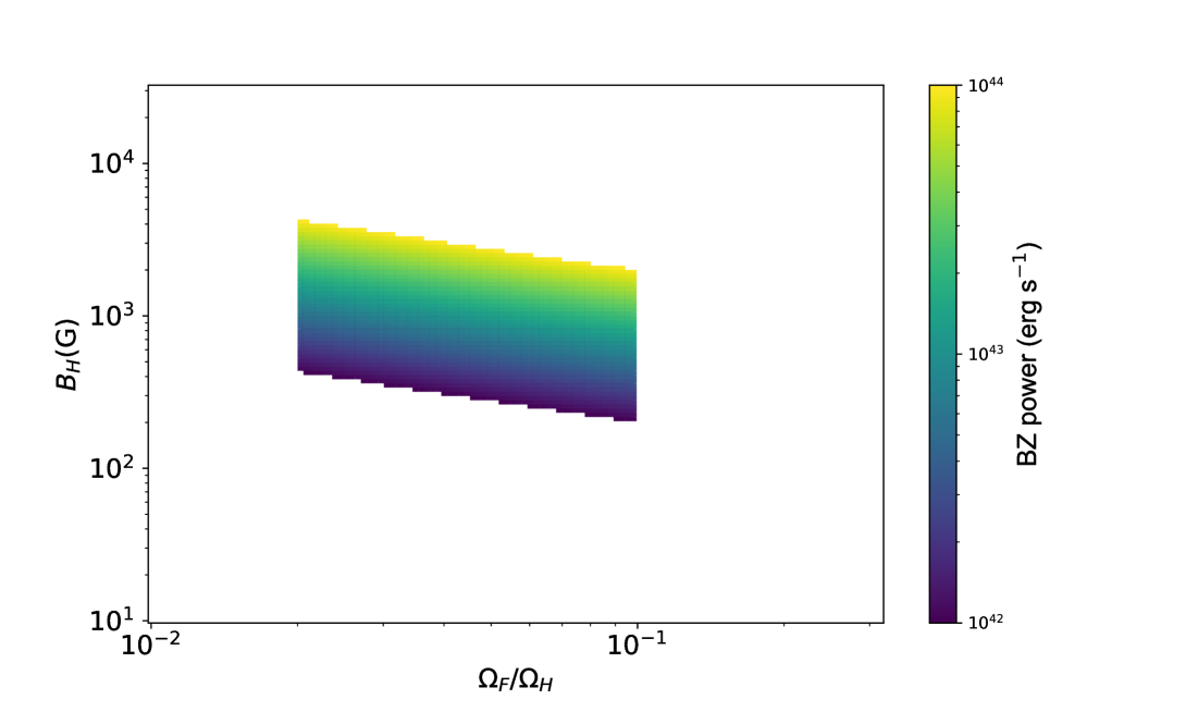
Figure 9: Estimate of the magnetic field strength threading the event horizon. The horizontal axis shows the ratio $\Omega_{F}/\Omega_{H}$ where $\Omega_{F}$ is constrained as Eq. (27). The estimate here is simply derived by equating $L_{\rm BZ}$ (Appendix) to the total jet power in M87 suggested as $1\times 10^{42}~{}{\rm erg~{}s^{-1}}\lesssim L_{\rm j}\lesssim 1\times 10^{44}~{}{\rm erg~{}s^{-1}}$. The color bar shows the corresponding $L_{\rm BZ}$.

Figure 9 presents the estimated range of $B_{\rm H}$ in the allowed range of $\Omega_{F}/\Omega_{H}$ together with the assumption of $L_{BZ}\approx L_{\rm j}$ which holds unless significant dissipation happens during its propagation. We conservatively allow a fairly wide range of the jet power as $1\times 10^{42}~{}{\rm erg~{}s^{-1}}\lesssim L_{\rm j}\lesssim 1\times 10^{44}~{}{\rm erg~{}s^{-1}}$ (e.g., Reynolds et al., 1996; Bicknell & Begelman, 1996; Owen et al., 2000; Stawarz et al., 2006; de Gasperin et al., 2012). Following the recent GRMHD simulations of highly magnetized jets (e.g., Porth et al., 2019; Ripperda et al., 2019), we set the value of the magnetic field threading angle as $\theta_{H}=1$ radian and it leads to $\chi=0.18$ (see Appendix). Then, the estimated $B_{H}$ lies in the range of $2\times 10^{2}~{}{\rm G}\lesssim B_{\rm H}\lesssim 4\times 10^{3}~{}{\rm G}$, which is comparable to the estimation by Blandford et al. (2019). This is larger than those estimated at the EHT photon ring region (Event Horizon Telescope Collaboration, 2019e; Event Horizon Telescope Collaboration et al., 2021; EHT MWL Science Working Group et al., 2021). The corresponding dimensionless magnetic flux on the event horizon scale ($\phi_{\rm BH}$) is estimated as $\phi_{\rm BH}\equiv(\Phi_{\rm BH}/\dot{M}r_{g}^{2}c)^{1/2}\approx 22(B_{H}/10^{3}~{}{\rm G})(\dot{M}/10^{-3}~{}{\rm M_{\odot}~{}yr^{-1}})^{-1/2}$ where $\Phi_{\rm BH}\approx B_{H}r_{g}^{2}$, and $\dot{M}$ are the magnetic flux threading the black hole, and the mass accretion rate onto the black hole, respectively. The mass accretion rate is adopted from (Event Horizon Telescope Collaboration et al., 2021). Accretion flows with $\phi_{\rm BH}\sim 1$ are classified as Standard and Normal Evolution (SANE: Narayan et al., 2012) state, while the accretion flows with a larger $\phi_{\rm BH}$ such as $\phi_{\rm BH}\gtrsim 15$ are conventionally referred as Magnetically Arrested Disks (MAD: Igumenshchev et al., 2003; Narayan et al., 2003; Tchekhovskoy et al., 2011; Event Horizon Telescope Collaboration, 2019e) state. The obtained $\phi_{\rm BH}$ obviously indicates that M87 is in a MAD regime. Although the estimation of the $B_{H}$ value depends on the adopted jet power, the estimated $\phi_{\rm BH}$ is consistent with the suggestion that M87 is MAD (Event Horizon Telescope Collaboration et al., 2021).

6.5.2 Consistency check with EHT results

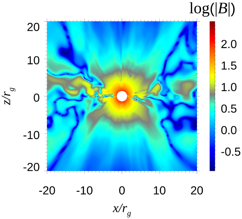
Figure 10: Map of magnetic field strength of a GRMHD simulation in logarithmic scale in a poloidal plane. Since GRMHD simulations are scale free, we normalized the mass accretion rate by carrying out GRRT calculations with RAIKOU code (Kawashima et al., 2019, 2021) using the parameters for M87* ($M_{\bullet}=6.5\times 10^{9}M_{\odot}$ and the distance $D=16.9$ Mpc in such a way that the resulting image reproduces the ring like image with the radiative flux $\sim 0.5$ Jy at 230 GHz observed by EHT (Event Horizon Telescope Collaboration, 2019a). Here we demonstrate the case of $B_{\rm H}=91$ G in the GRMHD simulation model This is roughly consistent with the $B_{\rm H}\gtrsim 200$ G estimated from our analytical jet model. Although the GRMHD simulation model shown here is in the semi-MAD state, we also confirmed that the MAD state achieved $B_{\rm H}\gtrsim 200$ G with the same procedure (Kawashima et al. in prep.) Although a detailed comparison with the EHT images is beyond the scope of this paper, it is clear that the reproduction of the photon-ring with the synchrotron flux density about 0.5 Jy at 230 GHz is feasible.

Since the averaged magnetic field strength at the photon-ring region is estimated as $B_{\rm ph-ring}\approx(5-30)~{}{\rm G}$ (Event Horizon Telescope Collaboration, 2019e; Event Horizon Telescope Collaboration et al., 2021; EHT MWL Science Working Group et al., 2021), at a glance, one may concern that a large $B_{H}$ may emit excess synchrotron radiation that largely exceeds the observed photon-ring flux about 0.5 Jy at 230 GHz. Therefore, it is worth to check whether the above estimated $B_{H}$ can be consistent with the EHT observation. To this end, it is straightforward to directly map magnetic field strengths at the jet base using GRMHD+GRRT simulation data. In Figure 10, we show an example of the mapping of magnetic field strength at the M87 jet base. We find that a case of relatively dimmer jet can make it possible to realize a large $B_{H}$ without violating the EHT observational results (see details for the model parameters in Appendix). Further detailed comparisons between the model and the observed images will be addressed as in future work.

7 Summary

Motivated by the measured velocity field profile of the M87 jet inthe KaVA large program by Park et al. (2019b) that shows a slower acceleration compared to those suggested by GRMHD simulations, we explore how to mitigate this apparent discrepancy by using a semi-analytic SRMHD jet model proposed by Tomimatsu & Takahashi (2003) consistently solving the trans-magnetic field structure. We summarize our findings as follows:

• By comparing TT03 model with the observed M87 jet velocity profile, we find that the model can reproduce the logarithmic feature of the velocity profile, and fit the observed data when choosing $c/(100r_{g})\lesssim\Omega_{F}\lesssim c/(70r_{g})$ which is by a factor of 7-10 slower than the typical $\Omega_{F}$ in GRMHD simulations (e.g., McKinney, 2006; Tchekhovskoy et al., 2010). We discussed the possibility that different boundary conditions lead to different values of $\Omega_{F}$.

• While a total specific energy (${\cal E}$) of each streamline changes the terminal bulk Lorentz factor, a slower angular velocity of the magnetic fields ($\Omega_{F}$) makes a light-cylinder radius ($r_{\rm lc}$) larger and it consequently push out a starting point of the jet acceleration. This provides us a new possibility to mitigate the apparent deviation between the KaVA observation of the M87 jet and GRMHD-simulation based prediction.

• By assuming Blandford-Znajek (BZ) process is in action with the total jet power of $10^{42-44}~{}{\rm erg~{}s^{-1}}$, we estimate the magnetic field strength on the event horizon scale in M87. Then, it is estimated as $2\times 10^{2}~{}{\rm G}\lesssim B_{H}\lesssim 5\times 10^{3}$ G for the total jet power of $10^{42-44}~{}{\rm erg~{}s^{-1}}$ in order to compensate for the effect of slower $\Omega_{F}$ than previously thought. The corresponding $\phi_{\rm BH}$ suggests that M87 is in a MAD regime. This is similar to the argument by Blandford et al. (2019) claiming the need of the spinning of the hole together with the magnetic field of order of $\sim 10^{3}$ G to launch the M87 jet.

• It is important to note that this work only discusses the extreme cases where dissipation does not work merely for simplicity. Although the simplification is basically justified to some extent (e.g., Chatterjee et al., 2019), it may be possible to have co-existence of a feeble dissipation at the jet base (e.g., Ripperda et al., 2020, 2021; Sironi et al., 2021). Inclusion of the magnetic reconnection process would probably facilitate to explain the observed characteristic limb brightening structure observed at 86 GHz (Hada et al., 2016; Kim et al., 2018). One of the ways to test this scenario would be to probe $u_{p}$ at the base of deeper jets ($\lesssim 10^{2}~{}r_{g}$) with VLBI observations of high spatial resolution and compare the model prediction by Takahashi et al. (2021) and those future VLBI observations.

Acknowledgment

We thank the referee for the comments that helped improve the overall clarity of the manuscript. We thank the EHT Collaboration internal reviewer Y. Mizuno, who carefully checked the manuscript and provided constructive comments. We are grateful to M. Nakamura and K. Toma for fruitful discussions and useful comments. We also thank K. Ohsuga and H. R. Takahashi for discussions on GRMHD simulations. This work was partially supported by the MEXT/JSPS KAKENHI (JP18H03721, JP17K05439, JP18K1359, JP21H01137, and JP22H00157). J.P. acknowledges financial support through the EACOA Fellowship awarded by the East Asia Core Observatories Association, which consists of the Academia Sinica Institute of Astronomy and Astrophysics, the National Astronomical Observatory of Japan, Center for Astronomical Mega-Science, Chinese Academy of Sciences, and the Korea Astronomy and Space Science Institute. This research was also supported by MEXT as “Program for Promoting Researches on the Supercomputer Fugaku” (Toward a unified view of the universe: from large scale structures to planets, JPMXP1020200109) and JICFuS.

In this Appendix, a brief note on the estimation of BZ power is presented where the background metric is written by Boyer-Lindquist coordinates. The electromagnetic energy flux from the horizon is generally given by $T^{\mu\nu}k_{\nu}=T^{r}_{0}$ where $T^{\mu\nu}$ is the stress-energy tensor, and $k_{\nu}$ is the time-like Killing vector. For axisymmetric case, the radial component of the electromagnetic energy flux is explicitly given by (Blandford & Znajek, 1977; Znajek, 1977)

$$T^{r}_{0} = -\epsilon_{0}\frac{\Omega_{F}B_{\phi}}{\Sigma_{H}\sin\theta}\Psi_{\theta}$$ (1)

$$= 2\epsilon_{0}M_{\bullet}r_{H}\Omega_{F}(\Omega_{H}-\Omega_{F})\left(\frac{\Psi_{\theta}}{\Sigma_{H}}\right)^{2},$$

where $a=J/M_{\bullet}=2M_{\bullet}\Omega_{H}r_{H}$, $J=M_{\bullet}\Omega_{H}r_{H}^{2}$, $r_{H}=M_{\bullet}+\sqrt{M_{\bullet}^{2}-a^{2}}$, and $\Omega_{H}$ are, the spin parameter, the angular momentum, the radius of the outer horizon, and the angular velocity of the Kerr BH, respectively. We also note that $\Sigma_{H}=r_{H}^{2}+a^{2}\cos^{2}\theta$ and the toroidal magnetic fields on the event horizon ($B_{\phi}$) is given by $B_{\phi}=\frac{[\Omega_{F}(r_{H}^{2}+a^{2})-a]\sin\theta}{\Sigma_{H}}A_{\phi,\theta}$. In this Appendix, we locally use the conventionally used magnetic flux function of $\Psi=\Psi_{\rm BH}\left(\frac{r}{M_{\bullet}}\right)^{p}(1-\cos\theta)$ where $p$ is the power-law index describing the field geometry and $\Psi_{\rm BH}$ is constant. The case of $p=0$ corresponds to the conical magnetic field (split monopole), while $p=1$ describes the parabolic one.

The net BZ power in the jet is obtained by integrating the EM energy flux evaluated at the event horizon, where magnetic fields are within the half opening angle of the foot-point of the black hole magnetosphere $\theta_{H}$. Then, the BZ power is given by

$$L_{\rm BZ} = \int^{2\pi}_{0}d\phi\int^{\theta_{H}}_{0}T^{r}_{0}\Sigma_{H}\sin\theta d\theta$$ (2)

$$= 2\pi\epsilon_{0}\left(\frac{r_{H}}{M_{\bullet}}\right)^{2p}\Psi_{\rm BH}^{2}\int^{\theta_{H}}_{0}\frac{2M_{\bullet}r_{H}}{\Sigma_{H}}\Omega_{F}(\Omega_{H}-\Omega_{F})\sin^{3}\theta d\theta.$$

Thus we obtain $L_{\rm BZ}\propto\Omega_{F}(\Omega_{H}-\Omega_{F})\Psi_{\rm BH}^{2}$ and hence a slow $\Omega_{F}$ leads to a smaller $L_{\rm BZ}$ (e.g., Tchekhovskoy et al., 2008; Beskin & Kuznetsova, 2000). Then the BZ power can be further written as

$$L_{\rm BZ}\approx 2\pi\epsilon_{0}\Psi_{\rm BH}^{2}\left(\frac{r_{H}}{M_{\bullet}}\right)^{2p}\left(\frac{a}{2M_{\bullet}r_{H}}\right)^{2}\frac{\Omega_{F}(\Omega_{H}-\Omega_{F})}{\Omega_{H}^{2}}\chi.$$ (3)

When the magnetic field geometry is split-monopole for instance, the BZ power is estimated as

$$L_{\rm BZ} \approx 7.5\times 10^{45}\chi_{-2}\frac{\Omega_{F}(\Omega_{H}-\Omega_{F})}{\Omega_{H}^{2}}\left(\frac{B_{H}}{10^{3}~{}{\rm G}}\right)^{2}\left(\frac{r_{H}}{10^{15}~{}{\rm cm}}\right)^{2}~{}{\rm erg~{}s^{-1}},$$ (4)

where $\Psi_{\rm BH}\approx B_{H}r_{H}^{2}$ is the magnetic flux on the horizon and here we omit $a$ dependence in $r_{H}$ merely for simplicity. The case of parabolic magnetic field geometry needs to multiply the additional factor of $r_{H}/M_{\bullet}=1+\sqrt{1-(a/M_{\bullet})^{2}}$, which maximally becomes the factor of 2 at most.

In this Appendix, we explain of one example of GRMHD simulation presented in the discussion in details. We used a GRMHD simulation snapshot in semi-MAD state with normalized spin parameter $a_{*}=0.9375$, which is same with that shown in (Kawashima et al., 2021) performed by using a GR(-Radiation)MHD simulation code UWABAMI (Takahashi et al., 2016). To set the electron temperature $T_{\rm e}$, we assumed an $R$-$\beta$ prescription (e.g., Mościbrodzka et al., 2016; Event Horizon Telescope Collaboration, 2019e) given by

$$\frac{T_{p}}{T_{e}}=R_{\rm high}\frac{\beta^{2}}{1+\beta^{2}}+R_{\rm low}\frac{1}{1+\beta^{2}}$$ (5)

where $T_{\rm p}$ and $\beta$ are the proton temperature and plasma beta (i.e., the ratio of gas pressure to magnetic pressure), respectively. The term $R_{\rm high}$ parameterizes $T_{e}$ in a high-$\beta$ accretion flow region, while $R_{\rm low}$ parameterizes $T_{e}$ in a low-$\beta$ jet region. By performing GRRT calculations with RAIKOU code (Kawashima et al., 2019, 2021), we search for combinations of $R_{low}$ and $B_{H}$ that satisfy the total flux about 0.5 Jy at 230 GHz(Event Horizon Telescope Collaboration, 2019a) and $B_{H}$ estimated in the present work. Following EHTC work, we conservatively choose $\sigma_{\rm cut}=1$ to fully exclude the emission coming from the density floor region. We set $R_{\rm high}=160$ and $R_{\rm low}=2$ where $R_{\rm low}$ is set to be slightly larger than that used in the most of works $R_{\rm low}=1$. The $R_{\rm low}$ larger than unity will be applicable, since the radiative cooling via synchrotron and inverse-Compton scattering processes can reduce the electron temperature and one temperature assumption in the low-$\beta$ region can breakdown (see, e.g., Figure 17 in Event Horizon Telescope Collaboration et al., 2021). In this work, we tried $R_{\rm low}$ than unity to examine the possibility of a large $B_{\rm H}$. This is because a larger mass accretion rate is required to reproduce the same radiative flux when $R_{\rm low}$ is larger (i.e., lower temperature in the highly magnetized region.). The magnetic field strength is proportional to the root square of the mass accretion rate in GRMHD simulations, i.e., the stronger magnetic field appears when we set a larger $R_{\rm low}$ with keeping reproducing the observed radiative flux. A large $R_{\rm low}$ reduces the 230 GHz flux density from the jet and thus can avoid the overshooting of the observed EHT flux density.

Figure 2: We show the $\Psi$ dependence of $u_{p}$ by drawing the $u_{p}$ profile with $\Psi=0.1\Psi_{0},0.2\Psi_{0},\dots,\Psi_{0}$. The fixed outer boundary wall has $q=1.3$.

Figure 4: We show the $\Omega$ dependence of $u_{p}$.

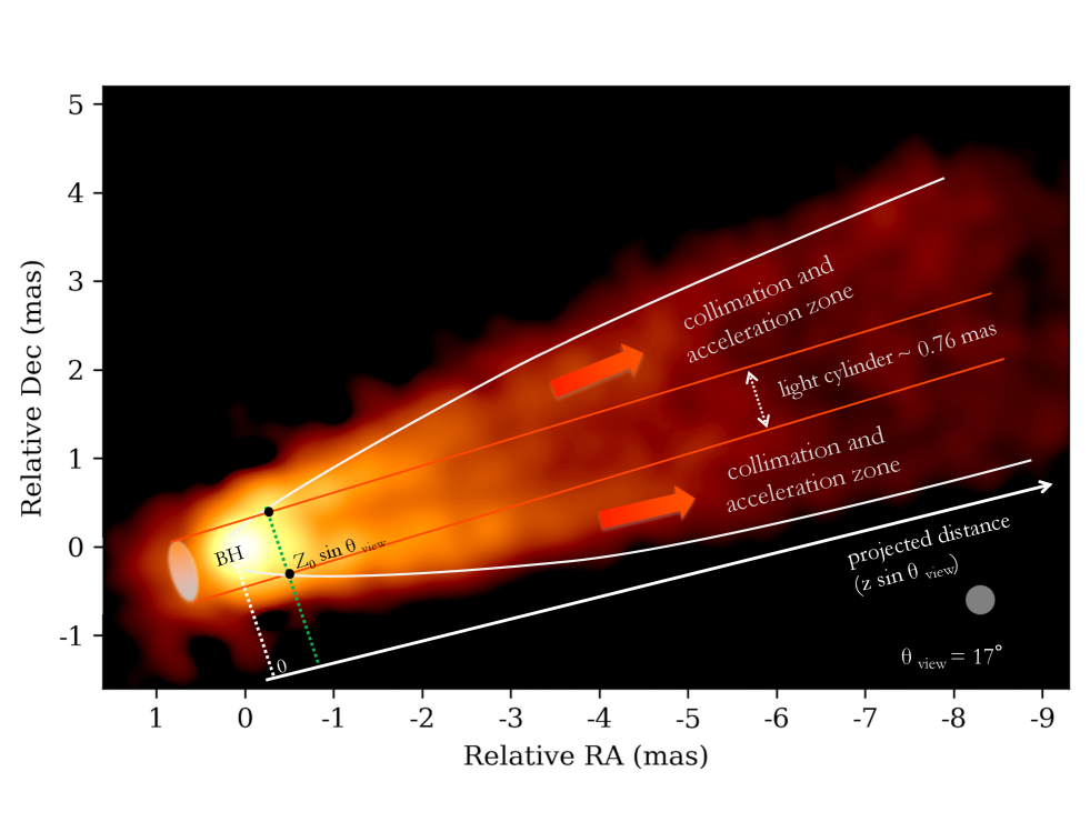
Figure 8: Schematic illustration of the model overlaid on stacked M87 image at 43 GHz (Cui et al. in preparation). TT03 model is applicable to the region outside the light cylinder. The model applicable range starts from $z\geq Z_{0}$, at which the outer boundary wall and the light cylinder have intersection points, and it is located at $\sim(2-4)\times 100~{}r_{g}$ from the central BH. As explained in the main body, the semi-parabolic boundary wall is determined by the jet-width measurement by VLBI (Asada & Nakamura, 2012; Hada et al., 2013).

References

- Abramowski et al. (2012) Abramowski, A., Acero, F., Aharonian, F., et al. 2012, ApJ, 746, 151, doi: 10.1088/0004-637X/746/2/151
- An et al. (2018) An, T., Sohn, B. W., & Imai, H. 2018, Nature Astronomy, 2, 118, doi: 10.1038/s41550-017-0277-z
- Asada & Nakamura (2012) Asada, K., & Nakamura, M. 2012, ApJ, 745, L28, doi: 10.1088/2041-8205/745/2/L28
- Asada et al. (2014) Asada, K., Nakamura, M., Doi, A., Nagai, H., & Inoue, M. 2014, ApJ, 781, L2, doi: 10.1088/2041-8205/781/1/L2
- Asada et al. (2017) Asada, K., Kino, M., Honma, M., et al. 2017, arXiv e-prints, arXiv:1705.04776. https://arxiv.org/abs/1705.04776
- Begelman & Li (1994) Begelman, M. C., & Li, Z.-Y. 1994, ApJ, 426, 269, doi: 10.1086/174061
- Beskin (2010) Beskin, V. S. 2010, MHD Flows in Compact Astrophysical Objects, doi: 10.1007/978-3-642-01290-7
- Beskin & Kuznetsova (2000) Beskin, V. S., & Kuznetsova, I. V. 2000, Nuovo Cimento B Serie, 115, 795. https://arxiv.org/abs/astro-ph/0004021
- Beskin et al. (1998) Beskin, V. S., Kuznetsova, I. V., & Rafikov, R. R. 1998, MNRAS, 299, 341, doi: 10.1046/j.1365-8711.1998.01659.x
- Bicknell & Begelman (1996) Bicknell, G. V., & Begelman, M. C. 1996, ApJ, 467, 597, doi: 10.1086/177636
- Biretta et al. (1999) Biretta, J. A., Sparks, W. B., & Macchetto, F. 1999, ApJ, 520, 621, doi: 10.1086/307499
- Blandford et al. (2019) Blandford, R., Meier, D., & Readhead, A. 2019, ARA&A, 57, 467, doi: 10.1146/annurev-astro-081817-051948
- Blandford & Znajek (1977) Blandford, R. D., & Znajek, R. L. 1977, MNRAS, 179, 433, doi: 10.1093/mnras/179.3.433
- Camenzind (1986) Camenzind, M. 1986, A&A, 162, 32
- Chatterjee et al. (2019) Chatterjee, K., Liska, M., Tchekhovskoy, A., & Markoff, S. B. 2019, MNRAS, 490, 2200, doi: 10.1093/mnras/stz2626
- Chen et al. (2018) Chen, A. Y., Yuan, Y., & Yang, H. 2018, ApJ, 863, L31, doi: 10.3847/2041-8213/aad8ab
- Cohen et al. (2014) Cohen, M. H., Meier, D. L., Arshakian, T. G., et al. 2014, ApJ, 787, 151, doi: 10.1088/0004-637X/787/2/151
- de Gasperin et al. (2012) de Gasperin, F., Orrú, E., Murgia, M., et al. 2012, A&A, 547, A56, doi: 10.1051/0004-6361/201220209
- Dexter et al. (2012) Dexter, J., McKinney, J. C., & Agol, E. 2012, MNRAS, 421, 1517, doi: 10.1111/j.1365-2966.2012.20409.x
- EHT MWL Science Working Group et al. (2021) EHT MWL Science Working Group, Algaba, J. C., Anczarski, J., et al. 2021, ApJ, 911, L11, doi: 10.3847/2041-8213/abef71
- Event Horizon Telescope Collaboration (2019a) Event Horizon Telescope Collaboration. 2019a, ApJ, 875, L1, doi: 10.3847/2041-8213/ab0ec7
- Event Horizon Telescope Collaboration (2019b) —. 2019b, ApJ, 875, L2, doi: 10.3847/2041-8213/ab0c96
- Event Horizon Telescope Collaboration (2019c) —. 2019c, ApJ, 875, L3, doi: 10.3847/2041-8213/ab0c57
- Event Horizon Telescope Collaboration (2019d) —. 2019d, ApJ, 875, L4, doi: 10.3847/2041-8213/ab0e85
- Event Horizon Telescope Collaboration (2019e) —. 2019e, ApJ, 875, L5, doi: 10.3847/2041-8213/ab0f43
- Event Horizon Telescope Collaboration (2019f) —. 2019f, ApJ, 875, L6, doi: 10.3847/2041-8213/ab1141
- Event Horizon Telescope Collaboration et al. (2021) Event Horizon Telescope Collaboration, Akiyama, K., Algaba, J. C., et al. 2021, ApJ, 910, L13, doi: 10.3847/2041-8213/abe4de
- Fishbone & Moncrief (1976) Fishbone, L. G., & Moncrief, V. 1976, ApJ, 207, 962, doi: 10.1086/154565
- Giroletti et al. (2012) Giroletti, M., Hada, K., Giovannini, G., et al. 2012, A&A, 538, L10, doi: 10.1051/0004-6361/201218794
- Hada et al. (2011) Hada, K., Doi, A., Kino, M., et al. 2011, Nature, 477, 185, doi: 10.1038/nature10387
- Hada et al. (2013) Hada, K., Kino, M., Doi, A., et al. 2013, ApJ, 775, 70, doi: 10.1088/0004-637X/775/1/70
- Hada et al. (2014) Hada, K., Giroletti, M., Kino, M., et al. 2014, ApJ, 788, 165, doi: 10.1088/0004-637X/788/2/165
- Hada et al. (2016) Hada, K., Kino, M., Doi, A., et al. 2016, ApJ, 817, 131, doi: 10.3847/0004-637X/817/2/131
- Hada et al. (2017) Hada, K., Park, J. H., Kino, M., et al. 2017, PASJ, 69, 71, doi: 10.1093/pasj/psx054
- Hawley & Krolik (2006) Hawley, J. F., & Krolik, J. H. 2006, ApJ, 641, 103, doi: 10.1086/500385
- Hirotani (2018) Hirotani, K. 2018, Galaxies, 6, 122, doi: 10.3390/galaxies6040122
- Hirotani & Okamoto (1998) Hirotani, K., & Okamoto, I. 1998, ApJ, 497, 563, doi: 10.1086/305479
- Hirotani & Pu (2016) Hirotani, K., & Pu, H.-Y. 2016, ApJ, 818, 50, doi: 10.3847/0004-637X/818/1/50
- Huang et al. (2020) Huang, L., Pan, Z., & Yu, C. 2020, ApJ, 894, 45, doi: 10.3847/1538-4357/ab86a3
- Igumenshchev et al. (2003) Igumenshchev, I. V., Narayan, R., & Abramowicz, M. A. 2003, ApJ, 592, 1042, doi: 10.1086/375769
- Junor et al. (1999) Junor, W., Biretta, J. A., & Livio, M. 1999, Nature, 401, 891, doi: 10.1038/44780
- Katsoulakos & Rieger (2020) Katsoulakos, G., & Rieger, F. M. 2020, ApJ, 895, 99, doi: 10.3847/1538-4357/ab8fa1
- Kawashima et al. (2019) Kawashima, T., Kino, M., & Akiyama, K. 2019, ApJ, 878, 27, doi: 10.3847/1538-4357/ab19c0
- Kawashima et al. (2021) Kawashima, T., Ohsuga, K., & Takahashi, H. R. 2021, arXiv e-prints, arXiv:2108.05131. https://arxiv.org/abs/2108.05131
- Kim et al. (2018) Kim, J.-Y., Lee, S.-S., Hodgson, J. A., et al. 2018, A&A, 610, L5, doi: 10.1051/0004-6361/201732421
- King & Pringle (2021) King, A. R., & Pringle, J. E. 2021, arXiv e-prints, arXiv:2107.12384. https://arxiv.org/abs/2107.12384
- Kino et al. (2015a) Kino, M., Niinuma, K., Zhao, G.-Y., & Sohn, B. W. 2015a, Publication of Korean Astronomical Society, 30, 633, doi: 10.5303/PKAS.2015.30.2.633
- Kino et al. (2015b) Kino, M., Takahara, F., Hada, K., et al. 2015b, ApJ, 803, 30, doi: 10.1088/0004-637X/803/1/30
- Kino et al. (2014) Kino, M., Takahara, F., Hada, K., & Doi, A. 2014, ApJ, 786, 5, doi: 10.1088/0004-637X/786/1/5
- Kisaka et al. (2020) Kisaka, S., Levinson, A., & Toma, K. 2020, ApJ, 902, 80, doi: 10.3847/1538-4357/abb46c
- Komissarov (2004) Komissarov, S. S. 2004, MNRAS, 350, 427, doi: 10.1111/j.1365-2966.2004.07598.x
- Komissarov (2021) —. 2021, MNRAS, doi: 10.1093/mnras/stab2686
- Komissarov et al. (2007) Komissarov, S. S., Barkov, M. V., Vlahakis, N., & Königl, A. 2007, MNRAS, 380, 51, doi: 10.1111/j.1365-2966.2007.12050.x
- Kovalev et al. (2007) Kovalev, Y. Y., Lister, M. L., Homan, D. C., & Kellermann, K. I. 2007, ApJ, 668, L27, doi: 10.1086/522603
- Kozlowski et al. (1978) Kozlowski, M., Jaroszynski, M., & Abramowicz, M. A. 1978, A&A, 63, 209
- Levinson & Cerutti (2018) Levinson, A., & Cerutti, B. 2018, A&A, 616, A184, doi: 10.1051/0004-6361/201832915
- Levinson & Globus (2016) Levinson, A., & Globus, N. 2016, MNRAS, 458, 2269, doi: 10.1093/mnras/stw459
- Levinson & Rieger (2011) Levinson, A., & Rieger, F. 2011, ApJ, 730, 123, doi: 10.1088/0004-637X/730/2/123
- Levinson & Segev (2017) Levinson, A., & Segev, N. 2017, Phys. Rev. D, 96, 123006, doi: 10.1103/PhysRevD.96.123006
- Lisakov et al. (2021) Lisakov, M. M., Kravchenko, E. V., Pushkarev, A. B., et al. 2021, ApJ, 910, 35, doi: 10.3847/1538-4357/abe1bd
- Lyubarsky (2009) Lyubarsky, Y. 2009, ApJ, 698, 1570, doi: 10.1088/0004-637X/698/2/1570
- MAGIC Collaboration et al. (2020) MAGIC Collaboration, Acciari, V. A., Ansoldi, S., et al. 2020, MNRAS, 492, 5354, doi: 10.1093/mnras/staa014
- McKinney (2006) McKinney, J. C. 2006, MNRAS, 368, 1561, doi: 10.1111/j.1365-2966.2006.10256.x
- Mertens et al. (2016) Mertens, F., Lobanov, A. P., Walker, R. C., & Hardee, P. E. 2016, A&A, 595, A54, doi: 10.1051/0004-6361/201628829
- Michel (1973) Michel, F. C. 1973, ApJ, 180, 207, doi: 10.1086/151956
- Mościbrodzka et al. (2016) Mościbrodzka, M., Falcke, H., & Shiokawa, H. 2016, A&A, 586, A38, doi: 10.1051/0004-6361/201526630
- Mościbrodzka et al. (2011) Mościbrodzka, M., Gammie, C. F., Dolence, J. C., & Shiokawa, H. 2011, ApJ, 735, 9, doi: 10.1088/0004-637X/735/1/9
- Murchikova et al. (2022) Murchikova, L., White, C. J., & Ressler, S. M. 2022, ApJ, 932, L21, doi: 10.3847/2041-8213/ac75c3
- Nakamura et al. (2018) Nakamura, M., Asada, K., Hada, K., et al. 2018, ApJ, 868, 146, doi: 10.3847/1538-4357/aaeb2d
- Narayan et al. (2003) Narayan, R., Igumenshchev, I. V., & Abramowicz, M. A. 2003, PASJ, 55, L69, doi: 10.1093/pasj/55.6.L69
- Narayan et al. (2012) Narayan, R., SÄ dowski, A., Penna, R. F., & Kulkarni, A. K. 2012, MNRAS, 426, 3241, doi: 10.1111/j.1365-2966.2012.22002.x
- Nathanail & Contopoulos (2014) Nathanail, A., & Contopoulos, I. 2014, ApJ, 788, 186, doi: 10.1088/0004-637X/788/2/186
- Niinuma et al. (2014) Niinuma, K., Lee, S.-S., Kino, M., et al. 2014, PASJ, 66, 103, doi: 10.1093/pasj/psu104
- Nitta (1997) Nitta, S.-Y. 1997, MNRAS, 284, 899, doi: 10.1093/mnras/284.4.899
- Ogihara et al. (2021) Ogihara, T., Ogawa, T., & Toma, K. 2021, ApJ, 911, 34, doi: 10.3847/1538-4357/abe61b
- Okino et al. (2021) Okino, H., Akiyama, K., Asada, K., et al. 2021, arXiv e-prints, arXiv:2112.12233. https://arxiv.org/abs/2112.12233
- Owen et al. (2000) Owen, F. N., Eilek, J. A., & Kassim, N. E. 2000, ApJ, 543, 611, doi: 10.1086/317151
- Parfrey et al. (2019) Parfrey, K., Philippov, A., & Cerutti, B. 2019, Phys. Rev. Lett., 122, 035101, doi: 10.1103/PhysRevLett.122.035101
- Park et al. (2019a) Park, J., Hada, K., Kino, M., et al. 2019a, ApJ, 871, 257, doi: 10.3847/1538-4357/aaf9a9
- Park et al. (2019b) —. 2019b, ApJ, 887, 147, doi: 10.3847/1538-4357/ab5584
- Penna et al. (2013) Penna, R. F., Narayan, R., & Sadowski, A. 2013, MNRAS, 436, 3741, doi: 10.1093/mnras/stt1860
- Porth et al. (2019) Porth, O., Chatterjee, K., Narayan, R., et al. 2019, ApJS, 243, 26, doi: 10.3847/1538-4365/ab29fd
- Pu et al. (2015) Pu, H.-Y., Nakamura, M., Hirotani, K., et al. 2015, ApJ, 801, 56, doi: 10.1088/0004-637X/801/1/56
- Pu & Takahashi (2020) Pu, H.-Y., & Takahashi, M. 2020, ApJ, 892, 37, doi: 10.3847/1538-4357/ab77ab
- Ressler et al. (2020a) Ressler, S. M., Quataert, E., & Stone, J. M. 2020a, MNRAS, 492, 3272, doi: 10.1093/mnras/stz3605
- Ressler et al. (2020b) Ressler, S. M., White, C. J., Quataert, E., & Stone, J. M. 2020b, ApJ, 896, L6, doi: 10.3847/2041-8213/ab9532
- Reynolds et al. (1996) Reynolds, C. S., Fabian, A. C., Celotti, A., & Rees, M. J. 1996, MNRAS, 283, 873, doi: 10.1093/mnras/283.3.873
- Ripperda et al. (2020) Ripperda, B., Bacchini, F., & Philippov, A. A. 2020, ApJ, 900, 100, doi: 10.3847/1538-4357/ababab
- Ripperda et al. (2021) Ripperda, B., Liska, M., Chatterjee, K., et al. 2021, arXiv e-prints, arXiv:2109.15115. https://arxiv.org/abs/2109.15115
- Ripperda et al. (2019) Ripperda, B., Bacchini, F., Porth, O., et al. 2019, ApJS, 244, 10, doi: 10.3847/1538-4365/ab3922
- Sikora et al. (2007) Sikora, M., Stawarz, Ł., & Lasota, J.-P. 2007, ApJ, 658, 815, doi: 10.1086/511972
- Sironi et al. (2021) Sironi, L., Rowan, M. E., & Narayan, R. 2021, ApJ, 907, L44, doi: 10.3847/2041-8213/abd9bc
- Stawarz et al. (2006) Stawarz, Ł., Aharonian, F., Kataoka, J., et al. 2006, MNRAS, 370, 981, doi: 10.1111/j.1365-2966.2006.10525.x
- Takahashi et al. (2016) Takahashi, H. R., Ohsuga, K., Kawashima, T., & Sekiguchi, Y. 2016, ApJ, 826, 23, doi: 10.3847/0004-637X/826/1/23
- Takahashi et al. (2018) Takahashi, K., Toma, K., Kino, M., Nakamura, M., & Hada, K. 2018, ApJ, 868, 82, doi: 10.3847/1538-4357/aae832
- Takahashi et al. (2021) Takahashi, M., Kino, M., & Pu, H.-Y. 2021, Phys. Rev. D, 104, 103004, doi: 10.1103/PhysRevD.104.103004
- Takahashi et al. (1990) Takahashi, M., Nitta, S., Tatematsu, Y., & Tomimatsu, A. 1990, ApJ, 363, 206, doi: 10.1086/169331
- Takahashi & Shibata (1998) Takahashi, M., & Shibata, S. 1998, PASJ, 50, 271, doi: 10.1093/pasj/50.2.271
- Takahashi & Tomimatsu (2008) Takahashi, M., & Tomimatsu, A. 2008, Phys. Rev. D, 78, 023012, doi: 10.1103/PhysRevD.78.023012
- Tchekhovskoy et al. (2008) Tchekhovskoy, A., McKinney, J. C., & Narayan, R. 2008, MNRAS, 388, 551, doi: 10.1111/j.1365-2966.2008.13425.x
- Tchekhovskoy et al. (2010) Tchekhovskoy, A., Narayan, R., & McKinney, J. C. 2010, ApJ, 711, 50, doi: 10.1088/0004-637X/711/1/50
- Tchekhovskoy et al. (2011) —. 2011, MNRAS, 418, L79, doi: 10.1111/j.1745-3933.2011.01147.x
- Thoelecke et al. (2019) Thoelecke, K., Takahashi, M., & Tsuruta, S. 2019, Progress of Theoretical and Experimental Physics, 2019, 093E01, doi: 10.1093/ptep/ptz097
- Thoelecke et al. (2017) Thoelecke, K., Tsuruta, S., & Takahashi, M. 2017, Phys. Rev. D, 95, 063008, doi: 10.1103/PhysRevD.95.063008
- Toma & Takahara (2012) Toma, K., & Takahara, F. 2012, ApJ, 754, 148, doi: 10.1088/0004-637X/754/2/148
- Toma & Takahara (2014) —. 2014, MNRAS, 442, 2855, doi: 10.1093/mnras/stu1053
- Tomimatsu (1994) Tomimatsu, A. 1994, PASJ, 46, 123
- Tomimatsu & Takahashi (2003) Tomimatsu, A., & Takahashi, M. 2003, ApJ, 592, 321, doi: 10.1086/375579
- Wajima et al. (2016) Wajima, K., Hagiwara, Y., An, T., et al. 2016, in Astronomical Society of the Pacific Conference Series, Vol. 502, Frontiers in Radio Astronomy and FAST Early Sciences Symposium 2015, ed. L. Qain & D. Li, 81
- Walker et al. (2018) Walker, R. C., Hardee, P. E., Davies, F. B., Ly, C., & Junor, W. 2018, ApJ, 855, 128, doi: 10.3847/1538-4357/aaafcc
- Wong et al. (2021) Wong, G. N., Ryan, B. R., & Gammie, C. F. 2021, ApJ, 907, 73, doi: 10.3847/1538-4357/abd0f9
- Zamaninasab et al. (2014) Zamaninasab, M., Clausen-Brown, E., Savolainen, T., & Tchekhovskoy, A. 2014, Nature, 510, 126, doi: 10.1038/nature13399
- Znajek (1977) Znajek, R. L. 1977, MNRAS, 179, 457, doi: 10.1093/mnras/179.3.457