Generalization Properties of NAS under Activation and Skip Connection Search

Abstract

Neural Architecture Search (NAS) has fostered the automatic discovery of state-of-the-art neural architectures. Despite the progress achieved with NAS, so far there is little attention to theoretical guarantees on NAS. In this work, we study the generalization properties of NAS under a unifying framework enabling (deep) layer skip connection search and activation function search. To this end, we derive the lower (and upper) bounds of the minimum eigenvalue of the Neural Tangent Kernel (NTK) under the (in)finite-width regime using a certain search space including mixed activation functions, fully connected, and residual neural networks. We use the minimum eigenvalue to establish generalization error bounds of NAS in the stochastic gradient descent training. Importantly, we theoretically and experimentally show how the derived results can guide NAS to select the top-performing architectures, even in the case without training, leading to a train-free algorithm based on our theory. Accordingly, our numerical validation shed light on the design of computationally efficient methods for NAS. Our analysis is non-trivial due to the coupling of various architectures and activation functions under the unifying framework and has its own interest in providing the lower bound of the minimum eigenvalue of NTK in deep learning theory.

1 Introduction

Neural Architecture Search (NAS) (Zoph and Le, 2017) is a powerful technique that enables the automatic design of neural architectures. NAS defines a set of operations (referred to as the search space), that include various activation functions and layer types, or potential connections among layers (Elsken et al., 2019; Ren et al., 2021). Optimization over the search space returns the optimal architecture as a subset of the possible combinations of operations. NAS obtains state-of-the-art results in image recognition (Liu et al., 2019a; Ding et al., 2020; Zhang et al., 2019; Chen et al., 2019) or can be used to further improve architectures defined by a human expert (Tan and Le, 2019). The spectacular results obtained by NAS have led to a significant interest in the community to further improve the NAS algorithms, the search space etc. However, to date little focus has been provided in the following question: Can NAS ¹ achieve generalization guarantees similar to a typical neural network?

Neural tangent kernel (NTK)-based analysis (Jacot et al., 2018) is a powerful method for analyzing the optimization and the generalization of deep networks (Allen-Zhu et al., 2019; Cao and Gu, 2019; Chen et al., 2020a; Arora et al., 2019a). The minimum eigenvalue of NTK has been used in previous work to demonstrate the global convergence of gradient descent, such as two-layer networks (Du et al., 2019b), and deep networks with polynomially wide layers (Allen-Zhu et al., 2019). Besides, the minimum eigenvalue of NTK is also used to prove generalization bounds (Arora et al., 2019a) and memorization (Montanari and Zhong, 2020). However, previous work mainly focuses on a limited set of architectures, e.g., fully-connected (FC) neural networks  (Allen-Zhu et al., 2018; Bartlett et al., 2017) or residual neural networks (He et al., 2016; Huang et al., 2020), in which a single activation function is used throughout the network. These off-the-shelf theoretical results cannot be directly applied to analyze the rich search space (of NAS) that is covering various/mixed architectures and parameters. That makes the non-trivial analysis on NAS worth of study on its own right.

The recent work of Oymak et al. (2021) is the first work to provide generalization guarantees on a related problem, i.e., activation functions search. The study provides generalization results on two-layer networks relying on the minimum eigenvalue with a strictly larger than zero assumption, i.e., $\lambda_{\min}(\bm{K})>0$ for the NTK matrix $\bm{K}$.

In this work, we introduce the first theoretical guarantees for multilayer NAS where the search space includes activation functions and skip connections. We study the upper/lower bound of the minimum eigenvalue of NTK (in the (in)finite regime) under mixed activation functions and architectures which evade the minimum eigenvalue assumption of Oymak et al. (2021). Then, we provide optimization and generalization guarantees of deep neural networks (DNNs) equipped with NAS. Our results indicate that the minimum eigenvalue estimation can act as a powerful metric for NAS. This method, called Eigen-NAS, is train-free, but still effective with experimental validation when compared to recent promising algorithms (Xu et al., 2021; Chen et al., 2021; Mellor et al., 2021). Formally, our main contribution and findings are summarized below:

i) We build a general theoretical framework based on NTK for NAS with search on popular activation functions in each layer, fully-connected, and skip connections. We derive the NTK formula of these architectures in the (in)finite-width regime under the unifying framework.

ii) We derive the upper and lower bounds of the minimum eigenvalue of the NTK under the (in)finite-width regime for the considered architectures. We introduce a new technique to ensure the probability of concentration inequality remains positive. Our analysis highlights how the upper and lower bounds differs under activation function search and skip connection search and can guide NAS.

iii) We establish a connection between the minimum eigenvalue and generalization of the searched DNN trained by stochastic gradient descent (SGD). Our theoretical results show that the generalization performance largely depends on the minimum eigenvalue of NTK for NAS, which provides theoretical guarantees for the searched architecture.

iv) Our theoretical results are supported by thorough experimental validations with the following findings: 1) our upper and lower bounds on the minimum eigenvalue largely depend on the activation function in the first layer rather than the activation functions in deeper layers. 2) The applied NAS algorithm always picks up ReLU (Rectified Linear Unit) and LeakyReLU in the optimal architecture, which coincides with our theory that predicts ReLU and LeakyReLU achieve the largest minimum eigenvalues. 3) The skip connections are required in each layer under our not very large DNNs. Furthermore, our experimental evidence on Eigen-NAS indicates that the minimum eigenvalue is a promising metric to guide NAS (without training) as suggested by our theory.

Technical challenges. The technical challenges of this paper mainly focus on how to analyze activation functions with different properties and skip connections under a unifying framework. This work is non-trivial; previous works mainly focus on the ReLU activation function (Nguyen et al., 2021; Cao and Gu, 2019; Allen-Zhu et al., 2019) in optimization and generalization of a single fully-connected neural network. Their proofs heavily depend on the properties of $\mathrm{ReLU}$, e.g., homogeneity and $\mathrm{ReLU}(x)=x\mathrm{ReLU}^{\prime}(x)$ which are invalid when other commonly-used activation functions, e.g., Tanh, Sigmoid, and Swish, are used. This problem becomes harder when mixed activation functions and residual connections are considered. To tackle these technical challenges, we develop the following techniques: a) to handle the non-homogeneous property of Tanh, Sigmoid, and Swish, we develop a new integral estimation approach for the minimal eigenvalue estimation. b) To establish the connection between the minimum eigenvalues of NTK and generalization errors, we use the Lipschitz continuity to avoid the special property of ReLU. More importantly, we introduce a new way to use Gershgorin circle theorem for minimum eigenvalue estimation, which avoids concentration inequalities with negative probability in some certain cases (Nguyen et al., 2021).

2 Related work

Network architecture search (NAS): The idea of NAS stems from Zoph and Le (2017), while the idea of cell search, i.e., searching core building blocks and composing them together, emerged in Zoph et al. (2018). The earlier literature used discrete optimization techniques for obtaining the architecture. DARTS (Liu et al., 2019b) considers NAS as a continuous bi-level optimization task. Recent variants of DARTS (Xu et al., 2019; Wu et al., 2019) and several train-free methods (Mellor et al., 2021; Chen et al., 2021; Xu et al., 2021) have demonstrated success in reducing the search time or improving the search algorithm. However, the aforementioned works have not provided generalization guarantees for the optimal architecture.

Optimization and generalization of DNNs via NTK: In the NTK framework (Jacot et al., 2018; Du et al., 2019a; Chen et al., 2020b), the training dynamics of (in)finite-width networks can be exactly characterized by kernel tools. Leveraging NTK facilitates studies on the global convergence of GD Allen-Zhu et al. (2019); Du et al. (2019a); Nguyen (2021) in DNNs via the minimum eigenvalue of NTK. In fact, it also controls the generalization performance of DNNs (Du et al., 2019b; Cao and Gu, 2019; Allen-Zhu et al., 2018), which is further studied in Bietti and Bach (2021).

3 Problem Settings

In this section we introduce the problem setting of our NAS framework based on the search space and algorithm (search strategy) for our paper.

Let $X\subseteq\mathbb{R}^{d}$ be a compact metric space and $Y\subseteq\mathbb{R}$. We assume that the training set $\mathcal{D}_{tr}=\{(\bm{x}_{i},y_{i})\}_{i=1}^{N}$ is drawn from a probability measure $\mathcal{D}$ on $X\times Y$, with its marginal data distribution denoted by $\mathcal{D}_{X}$. The goal of a supervised learning task is to find a hypothesis (i.e., a neural network used in this work) $f:X\rightarrow Y$ such that $f(\bm{x};\bm{W})$ parameterized by $\bm{W}$ is a good approximation of the label $y\in Y$ corresponding to a new sample $\bm{x}\in X$. In this paper, we consider the classification task, evaluated by minimizing the expected risk

$$\min_{\bm{W}}~{}\ell_{\mathcal{D}}(\bm{W}):=\mathbb{E}_{(\bm{x},y)\sim\mathcal{D}}~{}\ell[yf(\bm{x};\bm{W})]\,,$$

where $\ell[yf(\bm{x};\bm{W})]$ is the classification loss $\ell(\cdot)$ as a surrogate of the expected 0-1 loss $\ell_{\mathcal{D}}^{0-1}(\bm{W}):=\mathbb{E}_{(\bm{x},y)\sim\mathcal{D}}[1\left\{yf(\bm{x};\bm{W})<0\right\}]$. In this paper, we employ the cross-entropy loss, which is defined as $\ell(z)=\log[1+\exp(-z)]$.

Notation: For an integer $L$, we use the shorthand $[L]=\left\{1,2,\dots,L\right\}$. The multivariate standard Gaussian distribution is $\mathcal{N}(\bm{0},\mathbb{I}_{d})$ with the zero-mean vector $\bm{0}$ and the identity-variance matrix $\mathbb{I}_{d}$. We denote the direct sum by $\oplus$. We follow the standard Bachmann–Landau notation in complexity theory e.g., $\mathcal{O}$, $o$, $\Omega$, and $\Theta$ for order notation.

3.1 Neural Networks and Search Space

In this work, we consider a particular parametrization of $f$ as a deep neural network (DNN) with depth $L$ ($L\geq 3$) which includes the fully-connected (FC) neural networks setting and the residual neural networks setting, and various activation functions in each layer. This enables a quite general NAS setting. Formally, we define a single-output DNN with the output $\bm{f}_{l}(\bm{x})$ in each layer

$$\begin{matrix}\bm{f}_{l}(\bm{x})\!=\!\left\{\begin{matrix}\bm{x}&l=0\,,\\ \sigma_{1}(\bm{W}_{1}\bm{x})&l=1\,,\\ \sigma_{l}(\langle\bm{W}_{l},\bm{f}_{l-1}(\bm{x})\rangle)\!+\!\alpha_{l-1}\bm{f}_{l-1}(\bm{x})&2\!\leq\!l\!\leq\!L\!-\!1,\\ \left\langle\bm{W}_{L},\bm{f}_{L-1}(\bm{x})\right\rangle&l=L\,,\end{matrix}\right.\\ \end{matrix}$$ (1)

where the weights of the neural networks are $\bm{W}_{1}\in\mathbb{R}^{m\times d}$, $\bm{W}_{l}\in\mathbb{R}^{m\times m}$, $l=2,\dots,L-1$ and $\bm{W}_{L}\in\mathbb{R}^{m}$. The binary parameter $\alpha_{l}$ is for layer search, and the activation function is $\sigma_{l}(\cdot)$. The neural network output is $f(\bm{x};\bm{W})=f_{L}(\bm{x})$.

Architecture search: A binary vector $\bm{\alpha}=[\alpha_{1},\alpha_{2},\cdots,\alpha_{L-2}]^{\!\top}$ represents the skip connections, where the $\alpha_{l}\in\{0,1\}$ in Equation 1 indicates whether there is a skip connection in the $l$-th layer. Notice that we unify FC and residual neural networks under the same framework.

Activation function search: We select five representative activation functions defined by $\mathcal{F}_{\sigma}=\{\mathrm{ReLU},\mathrm{LeaklyReLU},\mathrm{Sigmoid},\mathrm{Tanh},\mathrm{Swish}\}$ used in Equation 1, that can be bounded, unbounded, smooth, non-smooth, monotonic, or non-monotonic, as reported in Table 1. We define $\bm{\sigma}=[\sigma_{1},\sigma_{2},\cdots,\sigma_{L-1}]^{\!\top}$ with $\sigma_{l}\in\mathcal{F}_{\sigma}$ for any $l\in[L-1]$ as the indicator to show which activation function is selected in each layer. Our NAS framework allows for a different activation function in each layer, which enlarges the search space.

In our setting, we conduct the architecture search and the skip connection search independently, and accordingly, our search space is defined as the direct sum of them:

$$\mathcal{W}:=\mathbb{R}^{L-2}\oplus\mathcal{F}_{\sigma}^{L-1}\oplus\{\mathbb{R}^{m\times d}\times(\mathbb{R}^{m\times m})^{L-2}\times\mathbb{R}^{m}\}\,,$$ (2)

where $\bm{W}:=(\bm{\alpha},\bm{\sigma},\bm{W}_{1},\dots,\bm{W}_{L})\in\mathcal{W}$ represents the collection of weight matrices and indicator for skips and selected activation functions for all layers.

Table 1: Formula of different activation functions, definitions of relevant constants and some intermediate results.

$\sigma_{l}$	ReLU	LeakyReLU	Sigmoid[1]	Tanh[2]	Swish
Formula	$\max(0,x)$	$\max(\eta x,x),~{}\eta\in(0,1)$	$\frac{1}{1+e^{-x}}-\frac{1}{2}$	$\frac{e^{x}-e^{-x}}{e^{x}+e^{-x}}$	$\frac{x}{1+e^{-x}}$
$\beta_{1}(\sigma_{l})$	$1$	$1+\eta^{2}$	$1/8$	$2$	$1$
$\beta_{2}(\sigma_{l})$	$1$	$1+\eta^{2}$	$1/8$	$2$	$1.22$
$\beta_{3}(\sigma_{l})$	$1$	$1+\eta^{2}$	$f_{S}(t)$	$f_{T}(t)$	$1/2$

• We consider the integral $f_{\mathrm{S}}(y)=\int_{-\infty}^{\infty}\frac{2}{\sqrt{2\pi y}}e^{-\frac{x^{2}}{2y}}{f^{\prime}_{\mathrm{Sigmoid}}}(x)^{2}\mathrm{d}x.$ We add $-1/2$ in Sigmoid to ensure $f_{\mathrm{Sigmoid}}(0)=0$ facilitates our theoretical analysis. The parameter is $t:=3(1+\eta^{2})(2+\eta^{2})^{L-3}$.

3.2 Algorithm (Search Strategy)

The search strategy is the core part in NAS to pick up the optimal architecture from the search space. Here we build a general Algorithm 1 combining the search strategy for NAS (the first part) and the subsequent neural network training by SGD (the second part).

We firstly utilize a typical NAS algorithm, e.g., random search WS (Li and Talwalkar, 2020) or DARTS, to search skip connections and activation functions independently, which results in the optimal architecture $\{(\sigma^{*}_{i})_{i=1}^{L-1},(\alpha^{*}_{i})_{i=1}^{L-2}\}$ with the max probability, see sec. 5.1 for details. In particular, Algorithm 1 also allows for the guidance of NAS in a train-free strategy via some specific metrics, e.g., the minimum eigenvalue of NTK (and its variant), see our Eigen-NAS method in sec. 5.2.

Then, we conduct neural network training on the selected architecture by SGD. For ease of theoretical analysis, we employ the constant step-size SGD with one epoch and randomly choose the weight parameters during all the iterations, which is commonly used in deep learning theory (Cao and Gu, 2019; Zou et al., 2019).

  Input: search space $\mathcal{S}$, data $\mathcal{D}_{tr}=\{(\bm{x}_{i},y_{i})_{i=1}^{N}\}$, step size $\gamma$ and ${\tt Flag}_{\mbox{\tiny method}}\in\left\{\tt EigenNAS,DARTS,\cdots\right\}$.

// conduct NAS algorithms

  if ${\tt Flag}_{\mbox{\tiny GuideNAS}}=\tt EigenNAS$ then

     Guide NAS from $\mathcal{S}$ by our Eigen-NAS algorithm.

  else if ${\tt Flag}_{\mbox{\tiny GuideNAS}}=\tt DARTS$ then

     Search neural network architectures from $\mathcal{S}$ using the DARTS algorithm.

  end if

  Output the optimal architecture $\{(\sigma^{*}_{i})_{i=1}^{L-1},(\alpha^{*}_{i})_{i=1}^{L-2}\}\in\mathcal{S}$ with max probability.

// do neural network training via SGD

  Gaussian initialization: $\bm{W}_{l}^{(1)}\sim\mathcal{N}(0,1/m)$, $l\in[L]$

  Construct the neural network $f(\bm{x};\bm{W}_{l}^{(1)})$ based on $\{(\sigma^{*}_{i})_{i=1}^{L-1},(\alpha^{*}_{i})_{i=1}^{L-2}\}$

  for $i=1$ to $N$ do

     $\bm{W}^{(i+1)}=\bm{W}^{(i)}-\gamma\cdot\nabla_{\bm{W}}\ell\big{(}f(\bm{x}_{i};\bm{W}^{(i)})y_{i}\big{)}\,.$

  end for

Output Randomly choose $\hat{\bm{W}}$ uniformly from $\left\{\bm{W}^{(1)},\dots,\bm{W}^{(N)}\right\}$.

Algorithm 1 SGD for training DNNs by NAS

4 Main result

In this section, we state the main theoretical results. We present the assumptions used in our proof in sec. 4.1. Then in sec. 4.2 we provide the recursive form of NTK for DNNs defined by Equation 1 with mixed activation functions and skip connections. The upper and lower bounds of the minimum eigenvalue of NTK in the infinite and finite-width setting is given in sec. 4.3 and 4.4, respectively. Finally, in sec. 4.5, we connect the minimum eigenvalue of NTK and the generalization error bound of DNNs under these search schemes. The proofs of our theoretical results presented in this section are deferred to Appendix B, C, and D, respectively.

4.1 Assumptions

We make the following assumptions on data and activation functions. Our assumptions are frequently employed in the literature as we highlight below.

Assumption 1.

The training data $\bm{x}_{1},\cdots,\bm{x}_{n}$ are i.i.d. sampling from a distribution under the $\ell_{2}$ normalization $\|\bm{x}_{i}\|_{2}=1$ for any $i\in[n]$. Besides, we assume that with probability 1, for any $i\neq j$, $\bm{x}_{i}\nparallel\bm{x}_{j}$, i.e., $\max_{i\neq j}\left\langle\bm{x}_{i},\bm{x}_{j}\right\rangle\leq C_{\max}<1$.

Assumption 2.

The activation function $\sigma:\mathbb{R}\rightarrow\mathbb{R}$ satisfies $\sigma\in L^{2}(\mathbb{R},e^{-x^{2}/2}/\sqrt{2\pi})$, where $L^{2}(\mathbb{R},g)$ denotes the square integrable function.

Remark: The first assumption on normalized data is commonly used in practice and theory on over-parameterized neural networks (Du et al., 2019b, a; Allen-Zhu et al., 2019; Oymak and Soltanolkotabi, 2020; Malach et al., 2020) and no parallel data points is standard in statistics and machine learning (Du et al., 2019b, a). The second assumption is general as the studied activation functions in Table 1 satisfy it.

4.2 Recursive NTK for DNNs defined by Equation 1

Recall that NTK (Jacot et al., 2018) under the infinite-width setting ($m\to\infty$) is:

$$K^{(L)}(\bm{x},\widetilde{\bm{x}}):=\mathbb{E}_{\bm{W}}\left\langle\frac{\partial f(\bm{x};\bm{W})}{\partial\bm{W}},\frac{\partial f(\widetilde{\bm{x}};\bm{W})}{\partial\bm{W}}\right\rangle\,,$$

where the NTK matrix for residual networks is derived by the following regular chain rule.

Lemma 1.

For any $l\in[3,L]$ and $s\in[2,L]$, denote

$$\small\begin{split}&\bm{G}^{(1)}=\bm{XX}^{\top}\,,\quad\bm{A}^{(2)}=\bm{G}^{(2)}=2\mathbb{E}_{\bm{w}\sim\mathcal{N}(\bm{0},\mathbb{I}_{d})}[\sigma_{1}(\bm{Xw})\sigma_{1}(\bm{Xw})^{\top}]\,,\\ &\bm{G}^{(l)}=2\mathbb{E}_{\bm{w}\sim\mathcal{N}(\bm{0},\mathbb{I}_{N})}[\sigma_{l-1}(\sqrt{\bm{A}^{(l-1)}}\bm{w})\sigma_{l-1}(\sqrt{\bm{A}^{(l-1)}}\bm{w})^{\top}]\,,\quad\bm{A}^{(l)}=\bm{G}^{(l)}+\alpha_{l-2}\bm{A}^{(l-1)}\,,\\ &\dot{\bm{G}}^{(s)}=2\mathbb{E}_{\bm{w}\sim\mathcal{N}(\bm{0},\mathbb{I}_{N})}[{\sigma}^{\prime}_{s-1}(\sqrt{\bm{A}^{(s-1)}}\bm{w}){\sigma}^{\prime}_{s-1}(\sqrt{\bm{A}^{(s-1)}}\bm{w})^{\top}]\,.\end{split}$$

Then the NTK for residual networks defined in Equation 1 can be written as

$$\bm{K}^{(L)}=\bm{G}^{(L)}+\sum_{l=1}^{L-1}\bm{G}^{(l)}\circ\dot{\bm{G}}^{(l+1)}\circ(\dot{\bm{G}}^{(l+2)}+\alpha_{l}\bm{1}_{N\times N})\circ\cdots\circ(\dot{\bm{G}}^{(L)}+\alpha_{L-2}\bm{1}_{N\times N})\,.$$

Remark: $(i)$ Our NTK formula of ResNet differs from the one of Tirer et al. (2022); Huang et al. (2020); Belfer et al. (2021) in two critical ways: 1) each skip-layer in our model skips one fully-connected layer and one activation function, as opposed to the two-layer skip of previous works, 2) our formulation does not require every layer to have a parallel skip connection, which increases the flexibility of the network. Those differences also result in a different NTK matrix.
$(ii)$ Our NTK formulation covers different activation functions, and we adopt the same initialization (coefficient) on them to ensure fair/equal search in our NAS framework.

Lemma 1 covers both FC and residual neural networks, which facilitates the analysis of the minimum eigenvalue of NTK under the unifying framework. If $\alpha_{l}=0$ for $l\in[L-1]$, our NTK formulation for residual neural networks degenerates to that of a fully connected neural network, and $\bm{A}^{l}$ and $\bm{G}^{l}$ become equal.

4.3 Minimum Eigenvalue of NTK for infinite-width

We are now ready to state the main result of the infinite-width neural network. We provide the upper and lower bounds of the minimum eigenvalue of NTK for an infinite-width neural network mixed with five different activation functions. The main differences between different activation functions are illustrated in Table 1.

Theorem 1.

For a DNN defined by Equation 1 and a not very large $L$, let $\bm{K}^{(L)}$ be the limiting NTK recursively defined in Lemma 1. Then, under Assumptions 1, choose $r\geq\frac{\log(2n)}{1-C_{\text{max}}}$, we have

$$\lambda_{\min}(\bm{K}^{(L)})\geq\mu_{r}(\sigma_{1})^{2}\prod_{p=3}^{L}\Bigg{(}\beta_{3}(\sigma_{p-1})+\alpha_{p-2}\Bigg{)}\,,$$

$$\lambda_{\min}(\bm{K}^{(L)})\leq\sum_{l=1}^{L}\Bigg{(}\beta_{1}(\sigma_{l-1})\prod_{p=2}^{l-1}\big{(}\beta_{1}(\sigma_{p-1})+\alpha_{p-2})\big{)}\prod_{p=l+1}^{L}(\beta_{2}(\sigma_{p-1})+\alpha_{p-2})\Bigg{)}\,,$$

where $\mu_{r}(\sigma_{1})$ is the $r$-st Hermite coefficient of the first layer activation function, and $\beta_{1},\beta_{2},\beta_{3}$ are three constants on various activation functions defined in Table 1.

Remark: A not very large depth, e.g., $L\leq 10$, is often sufficient for the search phase in practical implementations (Liu et al., 2018; Dong et al., 2021). In addition, existing NAS algorithms such as DARTS tend to have architectures with wide and shallow cell structures as suggested by Shu et al. (2020). Theorem 1 shows the upper and lower bounds of the minimum eigenvalue of NTK under the mix of activation functions and skip connections. The following conclusions can be drawn from our results:

1. The bounds of the minimum eigenvalue depend significantly on the depth of the network $L$, the skip connections via $\alpha_{p}$, which makes the minimum eigenvalue increase fast as $L$ and the number of skip connections increase. Besides, the minimum eigenvalue is also affected by activation functions via $\beta_{1},\beta_{2},\beta_{3}$. Nevertheless, the lower bound is independent of $\beta_{1}$ and $\beta_{2}$.

2. Different activation functions lead to different tendencies (increase or decrease) on $\lambda_{\min}(\bm{K}^{(L)})$. As the depth increases, the lower bound $\lambda_{\min}(\bm{K}^{(L)})$ under ReLU remains unchanged, increases under LeakyReLU, and decreases when Sigmoid, Tanh or Swish applied, which brings in new findings when compared to the ReLU-network analysis of Nguyen et al. (2021). For the upper bound for $\lambda_{\min}(\bm{K}^{(L)})$, we can see our results are positively correlated with the depth $L$.

3. One can see that $\mu_{1}(\sigma_{1})$ is only related to the activation function of the first layer, which implies that the activation function in the first layer is very important as $\lambda_{\min}(\bm{K}^{(L)})$ largely depends on it.

4.4 Minimum Eigenvalue of NTK for finite-width

To study the finite-width, we firstly introduce the Jacobian of the network. Let $\bm{F}=[f(\bm{x}_{1}),\ldots,f(\bm{x}_{N})]^{T}$. Then, the Jacobian $\bm{J}$ of $\bm{F}$ with respect to $\bm{W}$ is $\bm{J}=\left[\frac{\partial\bm{F}}{\partial\text{vec}(\bm{W}_{1})},\ldots,\frac{\partial\bm{F}}{\partial\text{vec}(\bm{W}_{L})}\right]$, where $\bm{J}$ have dimension $\mathbb{R}^{(((L-2)\times m+d+1)\times m\times N}$. The empirical Neural Tangent Kernel (NTK) matrix can be defined as $\bar{\bm{K}}^{(L)}=\bm{JJ}^{\top}=\sum_{l=1}^{L}\left[\frac{\partial\bm{F}}{\partial\text{vec}(\bm{W}_{l})}\right]\left[\frac{\partial\bm{F}}{\partial\text{vec}(\bm{W}_{l})}\right]^{\top}$.

Accordingly, we generalize Theorem 1 from the infinite-width to finite-width setting below.

Theorem 2.

For an $L$-layer network defined by Equation 1, let $\bm{K}^{(L)}=\bm{JJ}^{\top}$ be the NTK matrix, and the weights of the network be initialized as $[\bm{W}_{l}]_{i,j}\sim\mathcal{N}(0,1/m)$, for all $l\in[L]$. Under Assumptions 1, with probability at least $1-\sum_{l=1}^{L-1}\exp(-\Omega(m))-\exp(-\Omega(1))$, $\lambda_{\min}(\bm{JJ}^{\top})$ can be bounded by:

$$\Theta\bigg{(}\prod_{i=2}^{L-1}(\beta_{3}(\sigma_{i})+\alpha_{i-1})\bigg{)}\leq\lambda_{\min}(\bm{JJ}^{\top})\leq\sum_{k=0}^{L-1}\Theta\left(\prod_{i=k+2}^{L-1}(\beta_{2}(\sigma_{i})+\alpha_{i-1})\right)\,,$$

where the definitions of $\beta_{2}$, and $\beta_{3}$ are the same as those in Theorem 1.

Remark: Theorem 2 achieves a similar result as Theorem 1 if the width $m$ is large.

4.5 Connection to Generalization Error Bound

Based on the aforementioned upper and lower bounds of the minimum eigenvalue of NTK under different settings, here we establish its relationship with the generalization error of DNNs. We provide a bound on the expected 0-1 error obtained by Algorithm 1.

Theorem 3.

Given a DNN defined by Equation 1 with $\bm{y}=(y_{1},\dots,y_{N})^{\top}$ determined by Algorithm 1 with the step size of SGD $\gamma=\kappa C_{1}\cdot\sqrt{\bm{y}^{\top}({\bm{K}^{(L)}})^{-1}\bm{y}}/({m}\sqrt{N})$ for some small enough absolute constant $\kappa$. Under Assumptions 1 and 2, for any $\delta\in\left(0,e^{-1}\right]$ and a not very large $L$, if the width $m\geq\hat{m}$, where $\hat{m}$ depends on $\lambda_{\min}(\bm{K}^{(L)}),\delta,N$, and $L$, then with probability at least $1-\delta$ over the randomness of $\bm{W}^{(1)}$, we obtain the following high probability bound:

$$\mathbb{E}[\ell_{\mathcal{D}}^{0-\!1}\!(\hat{\bm{W}}\!)]\leq\tilde{\mathcal{O}}\left(\!C_{2}\sqrt{\frac{\bm{y}^{\top}({\bm{K}^{(L)}})^{-1}\bm{y}}{N}}\!\right)+\mathcal{O}\!\left(\sqrt{\frac{\log(1/\delta)}{N}}\right)\,,$$

where $C_{1}=\sqrt{L}/(3\mathrm{Lip}_{\max}+1)^{L-1}$ and $C_{2}=\sqrt{L}(3\mathrm{Lip}_{\max}+1)^{L-1}$ are two constants depending only on $L$ and $\mathrm{Lip}_{\max}$ is the maximum value of the Lipschitz constants of the all activation functions.

Remark: According to the courant minimax principle (Golub and Van Loan, 1996): $\frac{1}{\lambda_{\min}(\bm{K}^{(L)})}=\lambda_{\max}(({\bm{K}^{(L)}})^{-1})=\max\frac{\bm{y}^{\top}({\bm{K}^{(L)}})^{-1})\bm{y}}{\bm{y}^{\top}\bm{y}}$, that means $\bm{y}^{\top}(({\bm{K}^{(L)}})^{-1})\bm{y}\leq\frac{\bm{y}^{\top}\bm{y}}{\lambda_{\min}(\bm{K}^{(L)})}$, then the minimum eigenvalue plays a significant role in our analysis as well as our application on NAS. The quantity $\bm{y}^{\top}(({\bm{K}^{(L)}})^{-1})\bm{y}$ can be independent of $N$ in some certain cases (Arora et al., 2019a), leading to a classical $\mathcal{O}({N^{-1/2}})$ convergence rate for generalization.

Theorem 3 gives an algorithm-dependent generalization error bound of DNNs defined by Equation 1 trained with SGD with different activation functions and skip connections. If $m$ is large enough, the learning rate is infinitesimal, which means the generalization error bound mainly depends on the NTK matrix, similarly to Cao and Gu (2019); Du et al. (2019a). Admittedly, our result is in an exponential increasing order of the depth. However, in practice, the depth $L$ during the search phrase is smaller than $20$, or even $10$ (Liu et al., 2018; Dong et al., 2021). As we detail in Appendix E, our results extend previously known results.

According to Theorem 3, the generalization performance of DNNs is controlled by the minimum eigenvalue of the NTK matrix, which is in turn affected by different activation functions and skip connections, as discussed in Theorem 1. Apart from the NTK matrix itself, the condition $m\geq\hat{m}$ is also affected by different activation functions, which implies that the required minimum width is different in these cases.

4.6 Proof sketch

Our work extends the proofs of Nguyen and Mondelli (2020); Cao and Gu (2019) beyond ReLU, which is critical for enabling search across activations. The extension to other activation functions and skip connections is non-trivial due to non-linearity, inhomogeneity and nonmonotonicity.

To derive the upper and lower bounds on the minimum eigenvalue, we start from Lemma 1 on the NTK formula under the mixed activation functions and skip connections, and we transform the minimum eigenvalue estimation to the computation (estimation) of the bound $\bm{G}$, $\dot{\bm{G}}$ ($\lambda_{\min}(\bm{G})$). The infinite-width and finite-width are included in Appendix B and C respectively. For the upper bound, we estimate the diagonal elements of $\bm{G}$ and use the property that the minimum eigenvalue is less than the mean of the diagonal elements of a matrix to prove. For the lower bound, we use Hermite expansion. Combining these results concludes the proof.

To derive the generalization error bounds, we need a series of lemmas (see Appendix D). If the input weights are close, the output of each neuron with any activation function does not change too much (see Lemma 7). If the initilizations are close, the neural network output $f(\bm{x};\bm{W})$ is almost linear in $\bm{W}$ (see Lemma 8), and the loss function $\ell[y_{i}f(\bm{x}_{i};\bm{W})]$ is almost a convex function of $\bm{W}$ for any $i\in[N]$ (see Lemma 9). Accordingly, the gradient and loss of the neural network can be upper bounded by Lemmas 10 and 11, respectively, which concludes the proof when combined with some relevant results  (Cao and Gu, 2019; Allen-Zhu et al., 2019). Further discussion on the differences is deferred to Appendix E.

5 Numerical Validation

To validate our theoretical results, we conduct a series of experiments on NAS. Firstly, we simulate the NTK matrices under different depths in sec. F.4 to verify the relationship between the minimum eigenvalue of NTK and the network depth $L$ in Theorem 1. In sec. 5.1 we use the DARTS algorithm (Liu et al., 2019b) to conduct experiments on activation function search and skip connection search under the search space of Equation 1. Finally, we use the minimum eigenvalue of NTK to guide the training of NAS on the benchmark NAS-Bench-201 (Dong and Yang, 2020), with a comparison of recent NAS algorithms. Additional experiments on NAS-Bench-101 (Ying et al., 2019) and transfer learning are deferred to sec. F.5 and F.6.

5.1 DARTS experiment

In this section we employ a typical NAS algorithm, DARTS (Liu et al., 2019b), to assess our theoretical results on activation functions and skip connections. We select Fashion-MNIST (Xiao et al., 2017) as a standard benchmark. Details about Fashion-MNIST are shared in sec. F.1.

Search space and search strategy: Our search space is defined by Equation 2 on skip connections, activation functions, and weight parameters. We follow the search strategy of Liu et al. (2019b) in a two-level scheme, one level is for weight parameter search $\bm{W}$ and the other level is for architecture search $\{\bm{\alpha},\bm{\sigma}\}$, which results in the final optimal architecture $\{\bm{\alpha}^{*},\bm{\sigma}^{*},\bm{W}^{*}\}$. Different from Liu et al. (2019b), the activation function search and the skip connection search in our setting is independent. To obtain $\bm{\sigma}^{*}$, we use the softmax function to normalize the weights and choose the specific activation function with the highest probability in each layer. To obtain $\bm{\alpha}^{*}$, we initialize each entry $\alpha_{l}=1/2$ ($l\in[L-2]$), constrain it to $[0,1]$ during training, and retain the skip connection when $\alpha^{*}_{l}>1/2$.

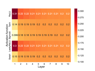
(a) activation functions $\bm{\sigma}$

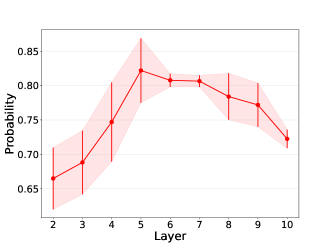
(b) skip connections $\bm{\alpha}$

Figure 1: Architecture search results on activation functions indicated by the probability of $\bm{\sigma}$ in (a) and skip connections indicated by $\bm{\alpha}$ in (b). We notice that for each layer, ReLU and LeakyReLU are selected a the higher probability.

Table 2: Results on CIFAR-10, CIFAR-100 and ImageNet-16 as part of NAS-Bench-201. The best performance is highlighted by bold. The results of NASWOT, TE-NAS and KNAS are reported from the corresponding papers. The results of ResNet, NAS-RL and DARTS are reported in  (Xu et al., 2021). The results illustrate that Eigen-NAS outperforms the prior art in CIFAR-100 and Imagenet-16. In particular, Eigen-NAS outperforms KNAS in all three cases when the same number of top-$k$ architectures are selected, i.e., $k=20$, and still achieves promising performance when smaller $k=5$ used, which we attribute to the more precise minimum eigenvalue estimation.

Type	Model/Algorithm	CIFAR-10 (%)	CIFAR-100 (%)	ImageNet-16 (%)
w/o Search	ResNet  (He et al., 2016)	$\bm{93.97}$	$70.86$	$42.63$
Search	NAS-RL  (Zoph and Le, 2017)	$92.83$	$70.71$	$44.10$
Gradient	DARTS  (Liu et al., 2019b)	$88.32$	$67.34$	$33.04$
Train-free	NASWOT  (Mellor et al., 2021)	$92.96$	$70.03$	$44.43$
Train-free	TE-NAS  (Chen et al., 2021)	$93.90$	$71.24$	$42.38$
Train-free	KNAS  (Xu et al., 2021) ($k=20$)	$93.38$	$70.78$	$44.63$
Train-free	NASI (T) (Shu et al., 2022)	$93.08\pm 0.24$	$69.51\pm 0.59$	$40.87\pm 0.85$
Train-free	NASI (4T) (Shu et al., 2022)	$93.55\pm 0.10$	$71.20\pm 0.14$	$44.84\pm 1.41$
Train-free	Eigen-NAS ($k=20$)	$93.46\pm 0.01$	$\bm{71.42}\pm 0.63$	$\bm{45.54}\pm 0.04$
Train-free	Eigen-NAS ($k=5$)	$93.43\pm 0.08$	$69.92\pm 1.82$	$45.53\pm 0.06$

NAS Results: We conduct the experiment via DARTS on a feedforward neural network with $L=10$ and $m=1024$, with 5 runs. After training, the probability of these activation functions and skip connections in each layer is reported in Figure 1(a) and 1(b), respectively. We have the following findings: Firstly, after the search process, LeakyReLU and ReLU are selected as the activations with the highest probability in each layer. This coincides with our theoretical results in Theorem 1. One minor difference is that the probability of LeakyReLU is slightly inferior to ReLU in practice. The reason behind this could be the sparsity of ReLU  (de Dios and Bruna, 2020). Secondly, in the first layer, we observe the largest difference on the probability of various activation functions. As the network becomes deeper, the differences decrease with the last layers having no difference between different activation functions. This phenomenon matches our theory well. To be specific, in Theorem 1, our result on the minimum eigenvalue largely depend on the first layer and its Hermite coefficient. Besides, this result also provides a justification on omitting the high-order terms while retaining the first layer activation terms. Thirdly, for the skip search result, we find that the skip connections are required in each layer when $L\leq 10$, as suggested by our theoretical results in Theorem 1. It also verifies the results of Zhou et al. (2020). We expect that the skip connections might not be required in each layer for deep neural networks, since their capacity can already be enough (He et al., 2016); but we defer the related study to a future work.

Interestingly, the search strategy favors the activation functions and the skip connections with larger minimum eigenvalue of NTK, which enjoy better generalization performance. This result also motivates us to study the following question: can the minimum eigenvalue of NTK guide the search process in NAS? We provide an affirmative answer in the next section with experimental validations.

5.2 NAS-Bench-201 Experiment

In this experiment, we use the minimum eigenvalue to guide NAS on NAS-Bench-201 (Dong and Yang, 2020). Each experiment is repeated 5 times, while it can run on a single GPU in a few hours.

Benchmark and baselines: NAS-Bench-201 (Dong and Yang, 2020) is a commonly used benchmark for NAS algorithm evaluation, which includes three datasets: a) CIFAR-10 (Krizhevsky et al., 2014), b) CIFAR-100 (Krizhevsky et al., 2014) and c) ImageNet-16  (Chrabaszcz et al., 2017) for image classification. Details on the datasets exist in sec. F.1. Apart from that, we evaluate the proposed approach with some baselines including ResNet, DARTS, RL based algorithm and some train-free algorithms.

Algorithm procedure: Our algorithm, called Eigen-NAS, also belongs in the train-free category. Eigen-NAS follows KNAS, which leverages the minimum eigenvalue of NTK to guide NAS. However, due to the $\mathcal{O}(N^{3})$ time complexity of computing these eigenvalues, KNAS instead computes $\|\bm{K}\|_{\mathrm{F}}$. However, from the expression $\lambda_{\min}(\bm{K})\leq\frac{1}{N}\sum_{i=1}^{N}K_{ii}\leq\|\bm{K}\|_{\mathrm{F}}$ we utilize the first inequality in Eigen-NAS to obtain a tighter (and more computationally efficient) bound to $\lambda_{\min}$. The computation cost of our method is $\mathcal{O}(N)$, which is less than computing the Frobenius norm ($\mathcal{O}(N^{2})$). Sequentially, the top-$k$ best candidates architectures are chosen in KNAS and our Eigen-NAS, and then the best architecture is chosen by the validation error. Please refer to the results in Table 2. Due to the page limit, the algorithm is located in Appendix F.

Results: The experimental results in Table 2 verify that Eigen-NAS guided by the proposed metric above achieves the best performance on both the CIFAR-100 and ImageNet-16 datasets, and competitive performance on CIFAR-10, outperforming KNAS in all three cases when $k=20$ for both methods. Even when we consider a smaller $k=5$, Eigen-NAS can outperform KNAS, which we attribute to the more precise minimum eigenvalue estimation.

6 Conclusion

In this work, we explore the relationship between the minimum eigenvalue of NTK and neural architecture search. We derive upper and lower bounds on the minimum eigenvalues of NTK for (in)finite residual networks under different mixtures of activation functions, and establish a connection between the minimum eigenvalues and the generalization properties of the special search space: activation function and skip connection search of NAS. Our theoretical results on various activation functions and mixed activation cases can also be a tool for deep learning theory researchers to prove generic results rather than studying a single architecture, e.g., ReLU networks. In addition, we use the minimum eigenvalue as a guide for the training of NAS in a train-free method, which greatly exceeds the efficiency of the classic NAS algorithm. When compared with existing train-free methods, our algorithm, called Eigen-NAS, achieves a higher accuracy. We posit that this will be useful for studying computationally efficient methods on NAS.

A core limitation is whether our proof framework can cover more general structures in NAS, such as the most commonly used convolutional neural networks (CNNs). Even though this seems possible, this is non-trivial due to the tensors that emerge. To be specific, it requires the element-recursive form of NTK matrices in Arora et al. (2019b) to be transformed into a global-recursive form (similar to Lemma 1), then analyze its minimum eigenvalue. Besides, the contraction operation of tensors, the locality and boundary effects of convolutional layer in CNNs make the analysis difficult. Therefore, we believe this is a topic on its own right. Another limitation of our work is that it does not analyze the various algorithms proposed for searching through the search space. We believe that a deeper understanding of such algorithms, such as DARTS can provide further insights into how to design improved search spaces. In addition, the upper and lower bounds of the minimum eigenvalues of the NTK matrices for different activation functions given by  Theorem 1 have some overlaps, which means that our suggestions on activation functions selection based on these bound appear a bit vacuous in theory but still coincide with our experimental validations. Maybe, a tighter bound without overlap for different activation functions is needed to address this theoretical issue.

Appendix introduction

The Appendix is organized as follows:

• In  Appendix A, we state the introductory notations and definitions.

• We prove Theorem 1 in Appendix B. We also provide the result when the residual network only has the same activation function.

• In Appendix C, we extend the results of infinitely width to finite-width and provide the proof for them.

• In Appendix D, we prove Theorem 3.

• In Appendix E, we discussion some key points of the proof and the motivation of the analysis.

• In Appendix F, we detail our experimental settings, our Eigen-NAS algorithm as used in sec. 5.2. We conduct additional numerical validations.

• Finally, in Appendix G, we discuss the societal impact of this work.

Appendix A Background

A.1 Symbols and Notation

In the paper, vectors are indicated with bold small letters, matrices with bold capital letters. To facilitate the understanding of our work, we include the some core symbols and notation in Table 3.

Table 3: Core symbols and notations used in this project.

Symbol	Dimension(s)	Definition
$\mathcal{N}(\mu,\sigma)$	-	Gaussian distribution of mean $\mu$ and variance $\sigma$
$1\left\{A\right\}$	-	Indicator function for event $A$
$[L]$	-	Shorthand of $\left\{1,2,\dots,L\right\}$
$\oplus$	-	Direct sum
$\mathcal{O}$, $o$, $\Omega$ and $\Theta$	-	Standard Bachmann–Landau order notation
$\circ$	-	Element-wise hadamard product
$\left\|\bm{v}\right\|_{2}$	-	Euclidean norms of vectors $\bm{v}$
$\left\|\bm{M}\right\|_{2}$	-	Spectral norms of matrices $\bm{M}$
$\left\|\bm{M}\right\|_{\mathrm{F}}$	-	Frobenius norms of matrices $\bm{M}$
$\left\|\bm{M}\right\|_{\mathrm{\ast}}$	-	Nuclear norms of matrices $\bm{M}$
$\lambda(\bm{M})$	-	Eigenvalues of matrices $\bm{M}$
$\bm{M}^{[l]}$	-	$l$-th row of matrices $\bm{M}$
$\bm{M}_{i,j}$	-	$(i,j)$-th element of matrices $\bm{M}$
$N$	-	Size of the dataset
$d$	-	Input size of the network
$L$	-	Depth of the network
$m$	-	Width of intermediate layer
$\alpha_{l}$	$\mathbb{R}$	A binary variable measures whether there is a skip connection in the $l$-th layer
$\sigma_{l}$	-	The activation function of $l$-th layer
$\beta_{1},\beta_{2},\beta_{3}$	$\mathbb{R},\mathbb{R},\mathbb{R}$	Three constants defined in Table 1
$\mu_{i}(\sigma)$	$\mathbb{R}$	The $i$-th Hermite coefficient of the activation function $\sigma$
$\bm{x}_{i}$	$\mathbb{R}^{d}$	The $i$-th data point
$y_{i}$	$\mathbb{R}$	The $i$-th target vector
$\bm{W}_{1}$	$\mathbb{R}^{m\times d}$	Weight matrix for the input layer
$\bm{W}_{l}$	$\mathbb{R}^{m\times m}$	Weight matrix for the $l$-th hidden layer
$\bm{W}_{L}$	$\mathbb{R}^{1\times m}$	Weight matrix for the output layer

A.1.1 Feature map

Here we define the core notation about feature maps that are required in the proof. Firstly, we define $\omega$-neighborhood to describe the difference between two matrices.

For any $\bm{W}\in\mathcal{W}$, we define its $\omega$-neighborhood as follows:

Definition 1 ($\omega$-neighborhood).

$$\mathcal{B}(\bm{W},\omega):=\left\{\bm{W}^{\prime}\in\mathcal{W}:\left\|\bm{W}^{\prime}_{l}-\bm{W}_{l}\right\|_{\mathrm{F}}\leq\omega,\bm{\alpha}^{\prime}=\bm{\alpha},\bm{\sigma}^{\prime}=\bm{\sigma},l\in[L]\right\}\,.$$

Then we define $(\bm{D}_{l})_{k,k}={\sigma_{l}}^{\prime}((\bm{W}_{l}\bm{f}_{l-1})_{k})$ as the back-propagation matrix of the activation function. We use the notation $\widetilde{\bm{W}}\in\mathcal{B}(\bm{W},\omega)$ to describe the relationship of the two matrices have $\omega$-neighborhood relationship.

In addition, we define the feature map of network and its perturbing matrix as follows:

Definition 2.

$$\small\begin{matrix}\widetilde{\bm{g}}_{i,1}=\widetilde{\bm{W}}_{1}\bm{x}_{i}\,,&\bm{g}_{i,1}=\bm{W}_{1}\bm{x}_{i}\,,&for\ i\in[N],\\ \widetilde{\bm{f}}_{i,1}=\sigma_{1}(\widetilde{\bm{W}}_{1}\bm{x}_{i})\,,&\bm{f}_{i,1}=\sigma_{1}(\bm{W}_{1}\bm{x}_{i})\,,&for\ i\in[N],\\ \widetilde{\bm{g}}_{i,l}=\widetilde{\bm{W}}_{l}\widetilde{\bm{f}}_{i,l-1}\,,&\bm{g}_{i,l}=\bm{W}_{l}\bm{f}_{i,l-1}\,,&for\ i\in[N]\ \text{and}\ l\!=\!2,\dots,L-1,\\ \widetilde{\bm{f}}_{i,l}=\sigma_{l}(\widetilde{\bm{W}}_{l}\widetilde{\bm{f}}_{i,l-1})+\alpha_{l-1}\widetilde{\bm{f}}_{i,l-1}\,,&\bm{f}_{i,l}=\sigma_{l}(\bm{W}_{l}\bm{f}_{i,l-1})+\alpha_{l-1}\bm{f}_{i,l-1}\,,&for\ i\in[N]\ \text{and}\ l\!=\!2,\dots,L-1\,.\end{matrix}$$

Let us define diagonal matrices $\widetilde{\bm{D}}_{i,l}\in\mathbb{R}^{m\times m}$ and $\bm{D}_{i,l}\in\mathbb{R}^{m\times m}$ by letting $(\widetilde{\bm{D}}_{i,l})_{k,k}={\sigma_{l}}^{\prime}((\widetilde{\bm{g}}_{i,l})_{k})$ and $(\bm{D}_{i,l})_{k,k}={\sigma_{l}}^{\prime}((\bm{g}_{i,l})_{k})$, $\forall k\in[m]$. Accordingly, we let $\hat{\bm{g}}_{i,l}=\widetilde{\bm{g}}_{i,l}-\bm{g}_{i,l}$, $\hat{\bm{f}}_{i,l}=\widetilde{\bm{f}}_{i,l}-\bm{f}_{i,l}$ and diagonal matrix $\hat{\bm{D}}_{i,l}=\widetilde{\bm{D}}_{i,l}-\bm{D}_{i,l}$.

A.1.2 Other notations

For the Hadamard product of the matrices $\bm{X}_{1},\bm{X}_{2},\cdots,\bm{X}_{r}$ that share the same dimensions, we use the following abbreviation:

$$\bigcirc_{i=1}^{r}(\bm{X}_{i})=\bm{X}_{1}\circ\bm{X}_{2}\circ\cdots\circ\bm{X}_{r}\,.$$

Appendix B The bound of the minimum eigenvalues of NTK for infinite-width

We present the details of our results on sec. 4.3 in this section. Firstly, we provide the proof of Theorem 1 in sec. B.2. Then in sec. B.3 we provide the result when several activation functions exist alone.

B.1 Proof of Lemma 1

Our proof mainly follows the results of Huang et al. [2020], but due to the different network structures, the proof process and results are slightly different. Moreover, we provide a matrix version results, which Huang et al. [2020] does not contain. For self-completeness, we include the proof here.

Proof.

By Huang et al. [2020, Proposition 3], written as matrix form,we have:

$$\begin{split}&\bm{A}^{(1)}=\bm{XX}^{\top}\,,\\ &\bm{A}^{(2)}=2\mathbb{E}_{\bm{w}\sim\mathcal{N}(\bm{0},\mathbb{I}_{d})}[\sigma_{1}(\bm{Xw})\sigma_{1}(\bm{Xw})^{\top}]\,,\\ &\bm{A}^{(l)}=2\mathbb{E}_{\bm{w}\sim\mathcal{N}(\bm{0},\mathbb{I}_{N})}[\sigma_{l-1}(\sqrt{\bm{A}^{(l-1)}}\bm{w})\sigma_{l-1}(\sqrt{\bm{A}^{(l-1)}}\bm{w})^{\top}]+\alpha_{l-2}\bm{A}^{(l-1)}\,.\end{split}$$

Note that, it is slightly different from the original result because the network structure is slightly different.

Let $\bm{G}^{(1)}=\bm{A}^{(1)}$, $\bm{G}^{(2)}=\bm{A}^{(2)}$ and $\bm{G}^{(l)}=2\mathbb{E}_{\bm{w}\sim\mathcal{N}(\bm{0},\mathbb{I}_{N})}[\sigma_{l-1}(\sqrt{\bm{A}^{(l-1)}}\bm{w})\sigma_{l-1}(\sqrt{\bm{A}^{(l-1)}}\bm{w})^{\top}]$, then we have:

$$\begin{split}&\bm{A}^{(1)}=\bm{G}^{(1)}=\bm{XX}^{\top}\,,\\ &\bm{A}^{(2)}=\bm{G}^{(2)}=2\mathbb{E}_{\bm{w}\sim\mathcal{N}(\bm{0},\mathbb{I}_{d})}[\sigma_{1}(\bm{Xw})\sigma_{1}(\bm{Xw})^{\top}]\,,\\ &\bm{G}^{(l)}=2\mathbb{E}_{\bm{w}\sim\mathcal{N}(\bm{0},\mathbb{I}_{N})}[\sigma_{l-1}(\sqrt{\bm{A}^{(l-1)}}\bm{w})\sigma_{l-1}(\sqrt{\bm{A}^{(l-1)}}\bm{w})^{\top}]\,,\\ &\bm{A}^{(l)}=\bm{G}^{(l)}+\alpha_{l-2}\bm{A}^{(l-1)}\,.\end{split}$$

According to Huang et al. [2020, Proposition 4], written as matrix form,we have:

$$\bm{K}^{(L)}=\sum_{l=1}^{L}\bm{G}^{(l)}\circ\dot{\bm{G}}^{(l+1)}\circ(\dot{\bm{G}}^{(l+2)}+\alpha_{l}\bm{1}_{N\times N})\circ\cdots\circ(\dot{\bm{G}}^{(L)}+\alpha_{L-2}\bm{1}_{N\times N})\,,$$

where the $\dot{\bm{G}}^{(s)}$ satisfy that $\dot{\bm{G}}^{(s)}=2\mathbb{E}_{\bm{w}\sim\mathcal{N}(\bm{0},\mathbb{I}_{N})}[{\sigma}^{\prime}_{s-1}(\sqrt{\bm{A}^{(s-1)}}\bm{w}){\sigma}^{\prime}_{s-1}(\sqrt{\bm{A}^{(s-1)}}\bm{w})^{\top}]$. Combining the above results, we finish the proof.

∎

B.2 Proof of Theorem 1

In this part, we present the proof of Theorem 1. Differently from Oymak and Soltanolkotabi [2020], our result allows for activation functions search in each layer.

Before we prove Theorem 1, we provide some propositions that are helpful to our proof. To facilitate the writing of the proof, let $\alpha_{0}:=0$.

Proposition 1.

When $\sigma_{1}$ is Tanh, the remaining layers are with LeakyReLU and for $l\in[L-2]$, $\alpha_{l}=1$, the quantity $G_{ii}^{(l)}$ has the largest upper bound:

$$G_{ii}^{(l)}\leq\begin{cases}1&\text{ if }l=1\\ 2(2+\eta^{2})^{l-2}&\text{ if }l\geq 2\,.\end{cases}$$ (3)

We set $G_{\max}=2(2+\eta^{2})^{L-2}$ as the upper bound of $G_{ii}^{(L)}$.

Proof.

To prove our result, we need bound $\bm{G}^{(l)}$ under different activation functions. We summarize them as below.

When $\sigma_{l-1}$ is ReLU:

$$\begin{split}G_{ii}^{(l)}&=2\mathbb{E}_{w\sim\mathcal{N}(0,A_{ii}^{(l-1)})}[\sigma_{l-1}(w)^{2}]=\int_{-\infty}^{\infty}\frac{2}{\sqrt{2\pi A_{ii}^{(l-1)}}}e^{-\frac{x^{2}}{2A_{ii}^{(l-1)}}}\max(0,x)^{2}\mathrm{d}x\\ &=\int_{0}^{\infty}\frac{2}{\sqrt{2\pi A_{ii}^{(l-1)}}}e^{-\frac{x^{2}}{2A_{ii}^{(l-1)}}}x^{2}\mathrm{d}x\\ &=A_{ii}^{(l-1)}\,.\end{split}$$ (4)

When $\sigma_{l-1}$ is LeakyReLU:

$$\begin{split}G_{ii}^{(l)}&=2\mathbb{E}_{w\sim\mathcal{N}(0,A_{ii}^{(l-1)})}[\sigma_{l-1}(w)^{2}]=\int_{-\infty}^{\infty}\frac{2}{\sqrt{2\pi A_{ii}^{(l-1)}}}e^{-\frac{x^{2}}{2A_{ii}^{(l-1)}}}\max(\eta x,x)^{2}\mathrm{d}x\\ &=\int_{0}^{\infty}\frac{2}{\sqrt{2\pi A_{ii}^{(l-1)}}}e^{-\frac{x^{2}}{2A_{ii}^{(l-1)}}}x^{2}\mathrm{d}x+\int_{-\infty}^{0}\frac{2}{\sqrt{2\pi A_{ii}^{(l-1)}}}e^{-\frac{x^{2}}{2A_{ii}^{(l-1)}}}\eta^{2}x^{2}\mathrm{d}x\\ &=(1+\eta^{2})A_{ii}^{(l-1)}\,.\end{split}$$ (5)

When $\sigma_{l-1}$ is Sigmoid:

$$\begin{split}G_{ii}^{(l)}&=2\mathbb{E}_{w\sim\mathcal{N}(0,A_{ii}^{(l-1)})}[\sigma_{l-1}(w)^{2}]=\int_{-\infty}^{\infty}\frac{2}{\sqrt{2\pi A_{ii}^{(l-1)}}}e^{-\frac{x^{2}}{2A_{ii}^{(l-1)}}}f_{\mathrm{Sigmoid}}(x)^{2}\mathrm{d}x\\ &\leq\int_{-\infty}^{\infty}\frac{2}{\sqrt{2\pi A_{ii}^{(l-1)}}}e^{-\frac{x^{2}}{2A_{ii}^{(l-1)}}}(\frac{1}{2})^{2}\mathrm{d}x\\ &=\frac{1}{2}\,.\end{split}$$ (6)

When $\sigma_{l-1}$ is Tanh:

$$\begin{split}G_{ii}^{(l)}&=2\mathbb{E}_{w\sim\mathcal{N}(0,A_{ii}^{(l-1)})}[\sigma_{l-1}(w)^{2}]=\int_{-\infty}^{\infty}\frac{2}{\sqrt{2\pi A_{ii}^{(l-1)}}}e^{-\frac{x^{2}}{2A_{ii}^{(l-1)}}}f_{\mathrm{Tanh}}(x)^{2}\mathrm{d}x\\ &\leq\int_{-\infty}^{\infty}\frac{2}{\sqrt{2\pi A_{ii}^{(l-1)}}}e^{-\frac{x^{2}}{2A_{ii}^{(l-1)}}}\mathrm{d}x\\ &=2\,.\end{split}$$ (7)

When $\sigma_{l-1}$ is Swish:

$$\small\begin{split}G_{ii}^{(l)}&=2\mathbb{E}_{w\sim\mathcal{N}(0,A_{ii}^{(l-1)})}[\sigma_{l-1}(w)^{2}]=\int_{-\infty}^{\infty}\frac{2}{\sqrt{2\pi A_{ii}^{(l-1)}}}e^{-\frac{x^{2}}{2A_{ii}^{(l-1)}}}f_{\mathrm{Swish}}(x)^{2}\mathrm{d}x\\ &=\int_{-\infty}^{\infty}\frac{2}{\sqrt{2\pi A_{ii}^{(l-1)}}}e^{-\frac{x^{2}}{2A_{ii}^{(l-1)}}}\frac{x^{2}}{(1+e^{-x})^{2}}\mathrm{d}x\\ &=\int_{0}^{\infty}\frac{2}{\sqrt{2\pi A_{ii}^{(l-1)}}}e^{-\frac{x^{2}}{2A_{ii}^{(l-1)}}}x^{2}\times\bigg{(}\frac{1}{(1+e^{-x})^{2}}+\frac{1}{(1+e^{x})^{2}}\bigg{)}\mathrm{d}x\\ &\leq\int_{0}^{\infty}\frac{2}{\sqrt{2\pi A_{ii}^{(l-1)}}}e^{-\frac{x^{2}}{2A_{ii}^{(l-1)}}}x^{2}\mathrm{d}x\\ &=A_{ii}^{(l-1)}\,.\end{split}$$ (8)

Combining Equations 4, 5, 6, 7 and 8 with Lemma 1 we draw the conclusion and finish the proof. ∎

Proposition 2.

The relationship between $A^{(l)}_{ii}$ and $A^{(l-1)}_{ii}$ for different activation functions can be summarized as Table 4 according to the difference of $\sigma_{l-1}$.

$\sigma_{l-1}$	ReLU	LeakyReLU	Sigmoid	Tanh	Swish
Upper bound	$1$	$1+\eta^{2}$	$\frac{1}{8}$	$2$	$1$
Lower bound	$1$	$1+\eta^{2}$	$(\frac{1}{2}-\frac{1}{2\sqrt{1+\frac{G_{\max}}{4}}})\frac{1}{G_{\max}}$	$(2-\frac{2}{\sqrt{1+G_{\max}}})\frac{1}{G_{\max}}$	$\frac{1}{2}$

Table 4: Upper and lower bounds for $A_{ii}^{(l)}/A_{ii}^{(l-1)}-\alpha_{l-2}$ for different activation functions $\sigma_{l-1}$ and the binary variable $\alpha_{l-2}\in\{0,1\}$ indicates whether $(l-1)$-th layer has a skip connection or not.

Proof.

To prove our result, we need to bound the ratio $A_{ii}^{(l)}/A_{ii}^{(l-1)}$ for different activation functions. We illustrate how this is achieved in different cases below:

For $l\geq 2$:

When $\sigma_{l-1}$ is ReLU by Equation 4 we have:

$$A_{ii}^{(l)}=G_{ii}^{(l)}+\alpha_{l-2}A_{ii}^{(l-1)}=(1+\alpha_{l-2})A_{ii}^{(l-1)}\,.$$ (9)

When $\sigma_{l-1}$ is LeakyReLU by Equation 5 we have:

$$A_{ii}^{(l)}=G_{ii}^{(l)}+\alpha_{l-2}A_{ii}^{(l-1)}=(1+\alpha_{l-2}+\eta^{2})A_{ii}^{(l-1)}\,.$$ (10)

When $\sigma_{l-1}$ is Swish, $G_{ii}^{(l)}$ can be upper by Equation 8 and lower bounded by:

$$\small\begin{split}G_{ii}^{(l)}&=2\mathbb{E}_{w\sim\mathcal{N}(0,A_{ii}^{(l-1)})}[\sigma_{l-1}(w)^{2}]=\int_{-\infty}^{\infty}\frac{2}{\sqrt{2\pi A_{ii}^{(l-1)}}}e^{-\frac{x^{2}}{2A_{ii}^{(l-1)}}}f_{\mathrm{Swish}}(x)^{2}\mathrm{d}x\\ &=\int_{-\infty}^{\infty}\frac{2}{\sqrt{2\pi A_{ii}^{(l-1)}}}e^{-\frac{x^{2}}{2A_{ii}^{(l-1)}}}\frac{x^{2}}{(1+e^{-x})^{2}}\mathrm{d}x\\ &=\int_{0}^{\infty}\frac{2}{\sqrt{2\pi A_{ii}^{(l-1)}}}e^{-\frac{x^{2}}{2A_{ii}^{(l-1)}}}x^{2}\times\bigg{(}\frac{1}{(1+e^{-x})^{2}}+\frac{1}{(1+e^{x})^{2}}\bigg{)}\mathrm{d}x\\ &\geq\int_{0}^{\infty}\frac{2}{\sqrt{2\pi A_{ii}^{(l-1)}}}e^{-\frac{x^{2}}{2A_{ii}^{(l-1)}}}x^{2}\times\frac{1}{2}\mathrm{d}x\\ &=\frac{1}{2}A_{ii}^{(l-1)}\,,\end{split}$$ (11)

which implies:

$$\left(\frac{1}{2}+\alpha_{l-2}\right)A_{ii}^{(l-1)}\leq A_{ii}^{(l)}\leq(1+\alpha_{l-2})A_{ii}^{(l-1)}\,.$$ (12)

When $\sigma_{l-1}$ is Sigmoid, $G_{ii}^{(l)}$ can be upper by:

$$\begin{split}G_{ii}^{(l)}&=2\mathbb{E}_{w\sim\mathcal{N}(0,A_{ii}^{(l-1)})}[\sigma_{l-1}(w)^{2}]=\int_{-\infty}^{\infty}\frac{2}{\sqrt{2\pi A_{ii}^{(l-1)}}}e^{-\frac{x^{2}}{2A_{ii}^{(l-1)}}}f_{\mathrm{Sigmoid}}(x)^{2}\mathrm{d}x\\ &\leq\int_{-\infty}^{\infty}\frac{2}{\sqrt{2\pi A_{ii}^{(l-1)}}}e^{-\frac{x^{2}}{2A_{ii}^{(l-1)}}}\bigg{(}\frac{1}{4}-e^{-\frac{x^{2}}{4}}\bigg{)}\mathrm{d}x=\frac{1}{2}-\frac{1}{2\sqrt{1+\frac{A_{ii}^{(l-1)}}{2}}}\\ &\leq\frac{A_{ii}^{(l-1)}}{8}\,,\quad\quad\quad\text{holds for $x\geq 0$}\,.\end{split}$$ (13)

Then $G_{ii}^{(l)}$ can be lower bounded by:

$$\begin{split}G_{ii}^{(l)}&=2\mathbb{E}_{w\sim\mathcal{N}(0,A_{ii}^{(l-1)})}[\sigma_{l-1}(w)^{2}]=\int_{-\infty}^{\infty}\frac{2}{\sqrt{2\pi A_{ii}^{(l-1)}}}e^{-\frac{x^{2}}{2A_{ii}^{(l-1)}}}f_{\mathrm{Sigmoid}}(x)^{2}\mathrm{d}x\\ &\geq\int_{-\infty}^{\infty}\frac{2}{\sqrt{2\pi A_{ii}^{(l-1)}}}e^{-\frac{x^{2}}{2A_{ii}^{(l-1)}}}\bigg{(}\frac{1}{4}-e^{-\frac{x^{2}}{8}}\bigg{)}\mathrm{d}x\\ &=\frac{1}{2}-\frac{1}{2\sqrt{1+\frac{A_{ii}^{(l-1)}}{4}}}\\ &\geq\left(\frac{1}{2}-\frac{1}{2\sqrt{1+\frac{G_{\max}}{4}}}\right)\frac{A_{ii}^{(l-1)}}{G_{\max}}\,,\end{split}$$ (14)

where we use the fact that the penultimate line is a concave function with respect to $A_{ii}^{(l-1)}$. When $A_{ii}^{(l-1)}=0$, the function value is 0. That means $G_{ii}^{(l)}/A_{ii}^{(l-1)}$ obtains the minimum value at $G_{ii}^{(l)}=G_{\max}$. Combined with Equation 3, we get the last inequality.

Then, we have:

$$\left(\left[\frac{1}{2}-\frac{1}{2\sqrt{1+\frac{G_{\max}}{4}}}\right]\frac{1}{G_{\max}}+\alpha_{l-2}\right)A_{ii}^{(l-1)}\leq A_{ii}^{(l)}\leq\left(\frac{1}{8}+\alpha_{l-2}\right)A_{ii}^{(l-1)}\,.$$ (15)

When $\sigma_{l-1}$ is Tanh, $G_{ii}^{(l)}$ can be upper bounded by:

$$\begin{split}G_{ii}^{(l)}&=2\mathbb{E}_{w\sim\mathcal{N}(0,A_{ii}^{(l-1)})}[\sigma_{l-1}(w)^{2}]=\int_{-\infty}^{\infty}\frac{2}{\sqrt{2\pi A_{ii}^{(l-1)}}}e^{-\frac{x^{2}}{2A_{ii}^{(l-1)}}}f_{\mathrm{Tanh}}(x)^{2}\mathrm{d}x\\ &\leq\int_{-\infty}^{\infty}\frac{2}{\sqrt{2\pi A_{ii}^{(l-1)}}}e^{-\frac{x^{2}}{2A_{ii}^{(l-1)}}}(1-e^{-x^{2}})\mathrm{d}x=2-\frac{2}{\sqrt{1+2A_{ii}^{(l-1)}}}\\ &\leq 2A_{ii}^{(l-1)}\,,\quad\quad\quad\text{holds for $x\geq 0$}\,.\end{split}$$ (16)

The lower bound is:

$$\begin{split}G_{ii}^{(l)}&=2\mathbb{E}_{w\sim\mathcal{N}(0,A_{ii}^{(l-1)})}[\sigma_{l-1}(w)^{2}]=\int_{-\infty}^{\infty}\frac{2}{\sqrt{2\pi A_{ii}^{(l-1)}}}e^{-\frac{x^{2}}{2A_{ii}^{(l-1)}}}f_{\mathrm{Tanh}}(x)^{2}\mathrm{d}x\\ &\geq\int_{-\infty}^{\infty}\frac{2}{\sqrt{2\pi A_{ii}^{(l-1)}}}e^{-\frac{x^{2}}{2A_{ii}^{(l-1)}}}(1-e^{-\frac{x^{2}}{2}})\mathrm{d}x\\ &=2-\frac{2}{\sqrt{1+A_{ii}^{(l-1)}}}\\ &\geq\bigg{(}2-\frac{2}{\sqrt{1+G_{\max}}}\bigg{)}\frac{A_{ii}^{(l-1)}}{G_{\max}}\,.\end{split}$$ (17)

Similar to the Sigmoid, the penultimate line is an concave function with respect to $A_{ii}^{(l-1)}$. When $A_{ii}^{(l-1)}=0$, the function value is 0. That means $G_{ii}^{(l)}/A_{ii}^{(l-1)}$ obtains the minimum value at $G_{ii}^{(l)}=G_{\max}$. Combined with Equation 3, we get the last inequality.

Then, we have:

$$\bigg{(}\bigg{[}2-\frac{2}{\sqrt{1+G_{\max}}}\bigg{]}\frac{1}{G_{\max}}+\alpha_{l-2}\bigg{)}A_{ii}^{(l-1)}\leq A_{ii}^{(l)}\leq(2+\alpha_{l-2})A_{ii}^{(l-1)}\,.$$ (18)

According to Equations 9, 10, 12, 15 and 18, we can summarized the results about bound of $A_{ii}^{(l)}/A_{ii}^{(l-1)}$ in Table 4.

∎

Proposition 3.

The bound of $\dot{G}^{(l)}_{ii}$ with respect to different activation function $\sigma_{l-1}$ can be summarized in Table 5.

$\sigma_{l-1}$	ReLU	LeakyReLU	Sigmoid	Tanh	Swish
Upper bound for $\dot{G}_{ii}^{(l)}$	$1$	$1+\eta^{2}$	$1/8$	$2$	$1.22$
Lower bound for $\dot{G}_{ii}^{(l)}$	$1$	$1+\eta^{2}$	$f_{\mathrm{S}}(G_{\max})$	$f_{\mathrm{T}}(G_{\max})$	$1/2$

Table 5: Upper and lower bounds for $\dot{G}_{ii}^{(l)}$ for different activation function $\sigma_{l-1}$.

Proof.

To prove our result, we need to bound $\dot{G}^{(l)}_{ii}$ with respect to different activation function $\sigma_{l-1}$ as follows.

When $\sigma_{l-1}$ is ReLU:

$$\begin{split}\dot{G}_{ii}^{(l)}&=2\mathbb{E}_{w\sim\mathcal{N}(0,A_{ii}^{(l-1)})}[{\sigma}^{\prime}_{l-1}(w)^{2}]=\int_{0}^{\infty}\frac{2}{\sqrt{2\pi A_{ii}^{(l-1)}}}e^{-\frac{x^{2}}{2A_{ii}^{(l-1)}}}\mathrm{d}x\\ &=1\,.\end{split}$$ (19)

When $\sigma_{l-1}$ is LeakyReLU:

$$\begin{split}\dot{G}_{ii}^{(l)}&=2\mathbb{E}_{w\sim\mathcal{N}(0,A_{ii}^{(l-1)})}[{\sigma}^{\prime}_{l-1}(w)^{2}]\\ &=\int_{0}^{\infty}\frac{2}{\sqrt{2\pi A_{ii}^{(l-1)}}}e^{-\frac{x^{2}}{2A_{ii}^{(l-1)}}}\mathrm{d}x+\int_{-\infty}^{0}\frac{2}{\sqrt{2\pi A_{ii}^{(l-1)}}}e^{-\frac{x^{2}}{2A_{ii}^{(l-1)}}}\eta^{2}\mathrm{d}x\\ &=1+\eta^{2}\,.\end{split}$$ (20)

When $\sigma_{l-1}$ is Sigmoid, according to the monotonicity of the $f_{\mathrm{S}}$, we have:

$$f_{\mathrm{S}}(G_{\max})\leq\dot{G}_{ii}^{(l)}=2\mathbb{E}_{w\sim\mathcal{N}(0,A_{ii}^{(l-1)})}[{\sigma}^{\prime}_{l-1}(w)^{2}]=f_{\mathrm{S}}(A_{ii}^{(l-1)})\leq f_{\mathrm{S}}(0)\leq\frac{1}{8}\,.$$ (21)

When $\sigma_{l-1}$ is Tanh, according to the monotonicity of the $f_{\mathrm{T}}$, we have:

$$f_{\mathrm{T}}(G_{\max})\leq\dot{G}_{ii}^{(l)}=2\mathbb{E}_{w\sim\mathcal{N}(0,A_{ii}^{(l-1)})}[{\sigma}^{\prime}_{l-1}(w)^{2}]=f_{\mathrm{T}}(A_{ii}^{(l-1)})\leq f_{\mathrm{T}}(0)\leq 2\,.$$ (22)

When $\sigma_{l-1}$ is Swish, The quantity $\dot{G}^{(l)}_{ii}$ can be upper bounded by:

$$\begin{split}\dot{G}_{ii}^{(l)}&=2\mathbb{E}_{w\sim\mathcal{N}(0,A_{ii}^{(l-1)})}[{\sigma}^{\prime}_{l-1}(w)^{2}]=\int_{-\infty}^{\infty}\frac{2}{\sqrt{2\pi A_{ii}^{(l-1)}}}e^{-\frac{x^{2}}{2A_{ii}^{(l-1)}}}f^{\prime}_{\mathrm{Swish}}(x)^{2}\mathrm{d}x\\ &\leq\int_{0}^{\infty}\frac{2}{\sqrt{2\pi A_{ii}^{(l-1)}}}e^{-\frac{x^{2}}{2A_{ii}^{(l-1)}}}\bigg{(}\sup_{x}f^{\prime}_{\mathrm{Swish}}(x)\bigg{)}^{2}\mathrm{d}x\\ &\quad+\int_{-\infty}^{0}\frac{2}{\sqrt{2\pi A_{ii}^{(l-1)}}}e^{-\frac{x^{2}}{2A_{ii}^{(l-1)}}}\bigg{(}\inf_{x}f^{\prime}_{\mathrm{Swish}}(x)\bigg{)}^{2}\mathrm{d}x\\ &=\bigg{(}\inf_{x}f_{\mathrm{Swish}}^{\prime}(x)\bigg{)}^{2}+\bigg{(}\sup_{x}f^{\prime}_{\mathrm{Swish}}(x)\bigg{)}^{2}\\ &\leq 1.22\,,\end{split}$$ (23)

where the last inequality holds by $1.099<\sup_{x}f^{\prime}_{\mathrm{Swish}}(x)<1.1$ and $-0.1<\inf_{x}f^{\prime}_{\mathrm{Swish}}(x)<-0.099$.

Then the quantity $\dot{G}^{(l)}_{ii}$ can be lower bounded by:

$$\begin{split}\dot{G}_{ii}^{(l)}&=2\mathbb{E}_{w\sim\mathcal{N}(0,A_{ii}^{(l-1)})}[{\sigma}^{\prime}_{l-1}(w)^{2}]=\int_{-\infty}^{\infty}\frac{2}{\sqrt{2\pi A_{ii}^{(l-1)}}}e^{-\frac{x^{2}}{2A_{ii}^{(l-1)}}}f^{\prime}_{\mathrm{Swish}}(x)^{2}\mathrm{d}x\\ &=\int_{0}^{\infty}\frac{2}{\sqrt{2\pi A_{ii}^{(l-1)}}}e^{-\frac{x^{2}}{2A_{ii}^{(l-1)}}}\bigg{(}f^{\prime}_{\mathrm{Swish}}(x)^{2}+f^{\prime}_{\mathrm{Swish}}(-x)^{2}\bigg{)}\mathrm{d}x\\ &\geq\int_{0}^{\infty}\frac{2}{\sqrt{2\pi A_{ii}^{(l-1)}}}e^{-\frac{x^{2}}{2A_{ii}^{(l-1)}}}\frac{1}{2}\mathrm{d}x\\ &=\frac{1}{2}\,.\end{split}$$ (24)

Combining Equations 19, 20, 21, 22, 23 and 24, we can summarize the results about bound of $\dot{G}_{ii}^{(l)}$ in Table 5.

∎

Now we are ready to prove Theorem 1.

Proof of Theorem 1.

Now we are ready to present the estimation on $\lambda_{\min}(\bm{K}^{(L)})$ as below.

From Lemma 1, we have the NTK formulation for residual neural networks:

$$\bm{K}^{(L)}=\bm{G}^{(L)}+\sum_{l=1}^{L-1}\bm{G}^{(l)}\circ\dot{\bm{G}}^{(l+1)}\circ(\dot{\bm{G}}^{(l+2)}+\alpha_{l}\bm{1}_{N\times N})\circ\cdots\circ(\dot{\bm{G}}^{(L)}+\alpha_{L-2}\bm{1}_{N\times N})\,.$$

It is clear that all the matrices $\bm{G}^{(l)}$, $\dot{\bm{G}}^{(l)}$ are positive semi-definite (PSD), then $(\dot{\bm{G}}^{(l+1)}+\alpha_{l}\bm{1}_{N\times N})$ are also PSD. For two PSD matrices $\bm{P},\bm{Q}\in\mathbb{R}^{N\times N}$, it holds $\lambda_{\min}(\bm{P}\circ\bm{Q})\geq\lambda_{\min}(\bm{P})\min_{i\in[N]}Q_{ii}$ [Schur, 1911] . Accordingly, we have:

$$\lambda_{\min}(\bm{K}^{(L)})\geq\sum_{l=1}^{L}\lambda_{\min}(\bm{G}^{(l)})\min_{i\in[N]}\prod_{p=l+1}^{L}\bigg{(}\dot{G}^{(p)}_{ii}+\alpha_{p-2}\bigg{)}\,.$$

Then we bound $\lambda_{\min}(\bm{G}^{(2)})$:

$$\begin{split}\lambda_{\min}(\bm{G}^{(2)})&=\lambda_{\min}\bigg{(}2\mathbb{E}_{\bm{w}\sim\mathcal{N}(0,\mathbb{I}_{d})}[\sigma_{1}(\bm{Xw})\sigma_{1}(\bm{Xw})^{\top}]\bigg{)}\\ &=2\lambda_{\min}\bigg{(}\sum_{s=0}^{\infty}\mu_{s}(\sigma_{1})^{2}\bigcirc_{i=1}^{s}(\bm{XX}^{\top})\bigg{)}\quad\text{\cite[citep]{[\@@bibref{AuthorsPhrase1Year}{NEURIPS2020_8abfe8ac}{\@@citephrase{, }}{}, Lemma D.3]}}\\ &\geq 2\mu_{r}(\sigma_{1})^{2}\lambda_{\min}(\bigcirc_{i=1}^{r}\bm{XX}^{\top})\quad\bigg{(}\mbox{taking~{}}r\geq\frac{\log(2N)}{1-C_{\text{max}}}\bigg{)}\\ &\geq 2\mu_{r}(\sigma_{1})^{2}\bigg{(}\min_{i\in[N]}\left\|\bm{x}_{i}\right\|_{2}^{2r}-(N-1)\max_{i\neq j}\left|\left\langle\bm{x}_{i},\bm{x}_{j}\right\rangle\right|^{r}\bigg{)}\quad\text{(Gershgorin circle theorem)}\\ &\geq 2\mu_{r}(\sigma_{1})^{2}\bigg{(}1-(N-1)C_{\text{max}}^{r}\bigg{)}\quad\left(\mbox{using~{}\lx@cref{creftype~refnum}{assumption:distribution_1}}\right)\\ &\geq 2\mu_{r}(\sigma_{1})^{2}\bigg{(}1-(N-1)\bigg{(}1-\frac{\log(2N)}{r}\bigg{)}^{r}\bigg{)}\\ &\geq 2\mu_{r}(\sigma_{1})^{2}\bigg{(}1-(N-1)\exp(-\log(2N))\bigg{)}\\ &\geq\mu_{r}(\sigma_{1})^{2}\,,\end{split}$$

where $\big{(}1-\frac{\log(2N)}{r}\big{)}^{r}$ is an increasing function of $r$ when $r\geq 2\log(2N)$. As a reminder, the symbol $\bigcirc$ denotes the Hadamard product, which is defined in sec. A.1.2.

That means:

$$\begin{split}\lambda_{\min}(\bm{K}^{(L)})&\geq\sum_{l=1}^{L}\lambda_{\min}(\bm{G}^{(l)})\min_{i\in[N]}\prod_{p=l+1}^{L}(\dot{G}^{(p)}_{ii}+\alpha_{p-2})\geq\lambda_{\min}(\bm{G}^{(2)})\min_{i\in[N]}\prod_{p=3}^{L}(\dot{G}^{(p)}_{ii}+\alpha_{p-2})\\ &\geq\mu_{r}(\sigma_{1})^{2}\min_{i\in[N]}\prod_{p=3}^{L}(\dot{G}^{(p)}_{ii}+\alpha_{p-2}),\quad\bigg{(}r\geq\frac{\log(2n)}{1-C_{\text{max}}}\bigg{)}\,.\end{split}$$ (25)

According to Table 1 and Table 5, we have:

$$\prod_{p=l+1}^{L}(\dot{G}^{(p)}_{ii}+\alpha_{p-2})\leq\prod_{p=l+1}^{L}\bigg{(}\beta_{2}(\sigma_{p-1})+\alpha_{p-2}\bigg{)}\,,$$ (26)

$$\prod_{p=3}^{L}(\dot{G}^{(p)}_{ii}+\alpha_{p-2})\geq\prod_{p=3}^{L}\bigg{(}\beta_{3}(\sigma_{p-1})+\alpha_{p-2}\bigg{)}\,.$$ (27)

We know that the sum of eigenvalues of $\bm{K}^{(L)}$ is equal to the trace of $\bm{K}^{(L)}$. The upper bound of $\lambda_{\min}(\bm{K}^{(L)})$ is directly given by:

$$\lambda_{\min}(\bm{K}^{(L)})\leq\frac{1}{N}\sum_{i=1}^{N}\sum_{l=1}^{L}(G^{(l)}_{ii})\prod_{p=l+1}^{L}(\dot{G}^{(p)}_{ii}+\alpha_{p-2})\,.$$ (28)

Final result - upper bound

For $G^{(l)}_{ii}$ we have the following bound:

$$\small G^{(l)}_{ii}=\beta_{1}(\sigma_{l-1})A^{(l-1)}_{ii}\leq\beta_{1}(\sigma_{l-1})\prod_{p=3}^{l-1}\bigg{(}\beta_{1}(\sigma_{p-1})+\alpha_{p-2}\bigg{)}A^{(2)}_{ii}\leq\beta_{1}(\sigma_{l-1})\prod_{p=2}^{l-1}\bigg{(}\beta_{1}(\sigma_{p-1})+\alpha_{p-2}\bigg{)}\,.$$ (29)

By Equations 26, 28 and 29, we have:

$$\lambda_{\min}(\bm{K}^{(L)})\leq\sum_{l=1}^{L}\bigg{(}\beta_{1}(\sigma_{l-1})\prod_{p=2}^{l-1}\bigg{[}\beta_{1}(\sigma_{p-1})+\alpha_{p-2}\bigg{]}\prod_{p=l+1}^{L}\bigg{[}\beta_{2}(\sigma_{p-1})+\alpha_{p-2}\bigg{]}\bigg{)}\,.$$ (30)

Final result - lower bound

By Equations 25 and 27, we have:

$$\lambda_{\min}(\bm{K}^{(L)})\geq\mu_{r}(\sigma_{1})^{2}\prod_{p=3}^{L}\bigg{(}\beta_{3}(\sigma_{p-1})+\alpha_{p-2}\bigg{)},\quad\bigg{(}r\geq\frac{\log(2n)}{1-C_{\text{max}}}\bigg{)}\,.$$

∎

B.3 Special cases

To provide further insights into our proofs of mixed activation functions as provided in the previous sections, we now consider the special case of a single activation function in each layer.

Corollary 4.

Under Assumption 1, for a deep fully-connected ResNet with the same activation functions in every layer and for a not very large $L$, let $\bm{K}^{(L)}$ be the limiting NTK recursively defined in Lemma 1. Then, we have:

For ReLU:

$$\mu_{r}(\sigma_{1})^{2}\prod_{p=3}^{L}(1+\alpha_{p-2})\leq\lambda_{\min}(\bm{K}^{(L)})\leq\sum_{l=1}^{L}\bigg{(}\frac{\prod_{p=2}^{L}(1+\alpha_{p-2})}{1+\alpha_{l-2}}\bigg{)}\,.$$

For LeakyReLU:

$$\mu_{r}(\sigma_{1})^{2}\prod_{p=3}^{L}(1+\eta^{2}+\alpha_{p-2})\leq\lambda_{\min}(\bm{K}^{(L)})\leq(1+\eta^{2})\sum_{l=1}^{L}\bigg{(}\frac{\prod_{p=2}^{L}(1+\eta^{2}+\alpha_{p-2})}{1+\eta^{2}+\alpha_{l-2}}\bigg{)}\,.$$

For Sigmoid:

$$\mu_{r}(\sigma_{1})^{2}\prod_{p=3}^{L}(f_{\mathrm{S}}(\frac{1}{2})+\alpha_{p-2})\leq\lambda_{\min}(\bm{K}^{(L)})\leq\frac{1}{8}\sum_{l=1}^{L}\bigg{(}\frac{\prod_{p=2}^{L}(\frac{1}{8}+\alpha_{p-2})}{\frac{1}{8}+\alpha_{l-2}}\bigg{)}\,.$$ (31)

For Tanh:

$$\mu_{r}(\sigma_{1})^{2}\prod_{p=3}^{L}(f_{\mathrm{T}}(2)+\alpha_{p-2})\leq\lambda_{\min}(\bm{K}^{(L)})\leq 2\sum_{l=1}^{L}\bigg{(}\frac{\prod_{p=2}^{L}(2+\alpha_{p-2})}{2+\alpha_{l-2}}\bigg{)}\,.$$ (32)

For Swish:

$$\mu_{r}(\sigma_{1})^{2}\prod_{p=3}^{L}(\frac{1}{2}+\alpha_{p-2})\leq\lambda_{\min}(\bm{K}^{(L)})\leq\sum_{l=1}^{L}\bigg{(}\prod_{p=2}^{l-1}(1+\alpha_{p-2})\prod_{p=l+1}^{L}(1.22+\alpha_{p-2})\bigg{)}\,.$$

The $\mu_{r}(\sigma_{1})$ is $r$-st Hermite coefficient of the activation function.

Proof.

By, Tables 1, 25 and 30. we can have this result.

It should be noted that for Sigmoid network (all of activation functions are Sigmoid) and Tanh (all of activation functions are Tanh) network, the upper bound of $G_{\max}$ will change. By Equations 6 and 7 we have for Sigmoid $G_{\max}=\frac{1}{2}$, For Tanh $G_{\max}=2$. That means $f_{\mathrm{S}}(G_{\max})$ in the Theorem 1 is replaced by $f_{\mathrm{S}}(\frac{1}{2})$ in Equation 31 and $f_{\mathrm{T}}(G_{\max})$ in the Theorem 1 is replaced by $f_{\mathrm{T}}(2)$ in Equation 32.

∎

Appendix C The bound of the minimum eigenvalues of NTK for finite-width

We present the details of our results on sec. 4.4 in this section. Firstly, we introduce the specific expression form for NTK of finite-width network in sec. C.1. Then, we introduce some lemmas in sec. C.2 to facilitate the proof of theorems, after that we provide the results of multiple activation functions are mixed in one network in sec. C.3 directly, finally we discuss the results.

C.1 Neural Tangent Kernel for finite-width

$$\bar{\bm{K}}^{(L)}=\bm{JJ}^{\top}=\sum_{l=1}^{L}\bigg{[}\frac{\partial\bm{F}}{\partial\mathrm{vec}(\bm{W}_{l})}\bigg{]}\bigg{[}\frac{\partial\bm{F}}{\partial\mathrm{vec}(\bm{W}_{l})}\bigg{]}^{\top}\,.$$

Let $\bm{F}_{k}=[\bm{f}_{k}(\bm{x}_{1}),\ldots,\bm{f}_{k}(\bm{x}_{N})]^{T}$, by chain rule and some standard calculation, we have,

$$\bm{JJ}^{\top}=\sum_{k=0}^{L-1}\bm{F}_{k}\bm{F}_{k}^{\top}\circ\bm{B}_{k+1}\bm{B}_{k+1}^{\top}\,,$$

where $\bm{B}_{k}\in\mathbb{R}^{N\times m}$ is a matrix of which the $i$-th row is given by

$$(\bm{B}_{k})_{i:}=\left\{\begin{matrix}\bm{D}_{i,k}\prod_{l=k+1}^{L-1}(\bm{W}_{l}\bm{D}_{i,l}+\alpha_{l-1}\bm{I}_{m\times m})\bm{W}_{L},k\in[L-2]\,,\\ \bm{D}_{i,L-1}\bm{W}_{L},\qquad\qquad\qquad\qquad\qquad\qquad k=L-1\,,\\ 1,\qquad\qquad\qquad\qquad\qquad\qquad\qquad\ \ k=L\,.\end{matrix}\right.$$

C.2 Relevant Lemmas

Lemma 2.

Fix any $k\in[0,L-1]$ and $\bm{x}\sim P_{X}$, then for ReLU, LeakyReLU, Sigmoid, Tanh and Swish we have

$$\left\|\bm{f}_{k}(\bm{x})\right\|_{2}^{2}=\Theta(1)\,,$$

with probability at least $1-\sum_{l=1}^{k}\exp(-\Omega(m))$ over $(\bm{W}_{l})_{l=1}^{k}$ and $\bm{x}$. Moreover,

$$\mathbb{E}_{\bm{x}}\left\|\bm{f}_{k}(\bm{x})\right\|_{2}^{2}=\Theta(1)\,,$$

with probability at least $1-\sum_{l=1}^{k-1}\exp(-\Omega(m))$ over $(\bm{W}_{l})_{l=1}^{k}$.

Proof.

We prove this by induction.

The result holds for $k=0$ due to 1.

Assume that the lemma holds for some $k-1$, i.e.

$$\left\|\bm{f}_{k-1}(\bm{x})\right\|_{2}^{2}=\Theta(1)\,,$$

with probability at least $1-\sum_{l=1}^{k-1}\exp(-\Omega(m))$ over $(\bm{W}_{l})_{l=1}^{k}$ and $\bm{x}$.

Let us condition on this event of $(\bm{W}_{l})_{l=1}^{k-1}$ and study probability bounds over $\bm{W}_{k}$: Let $\bm{W}_{k}=\left[\bm{w}_{1},\cdots,\bm{w}_{m}\right]^{\top}$ where $\bm{w}_{j}\sim\mathcal{N}(0,\mathbb{I}_{m}/m)$ and $f_{k}^{[j]}$ represents the $j$-th element of $\bm{f}_{k}$. Note that:

$$\left\|\bm{f}_{k}(\bm{x})\right\|_{2}^{2}=\sum_{j=1}^{m}f_{k}^{[j]}(\bm{x})^{2}\,.$$ (33)

Then we have:

$$\begin{split}\mathbb{E}_{\bm{W}_{k}}\left\|\bm{f}_{k}(\bm{x})\right\|_{2}^{2}&=\sum_{j=1}^{m}\mathbb{E}_{\bm{w}_{j}}[f_{k}^{[j]}(\bm{x})^{2}]\\ &=\sum_{j=1}^{m}\mathbb{E}_{\bm{w}_{j}}\bigg{(}\bigg{[}\sigma_{k}\bigg{(}\left\langle\bm{w}_{j},\bm{f}_{k-1}(\bm{x})\right\rangle\bigg{)}+\alpha_{k-1}f_{k-1}^{[j]}(\bm{x})\bigg{]}^{2}\bigg{)}\quad\quad~{}\lx@cref{creftype~refnum}{eq:network}\\ &=\sum_{j=1}^{m}\bigg{(}\mathbb{E}_{\bm{w}_{j}}\bigg{[}\bigg{(}\sigma_{k}(\left\langle\bm{w}_{j},\bm{f}_{k-1}(\bm{x})\right\rangle\bigg{)}^{2}\bigg{]}+\mathbb{E}_{\bm{w}_{j}}\bigg{(}\alpha_{k-1}^{2}f_{k-1}^{[j]}(\bm{x})^{2}\bigg{)}\\ &+\mathbb{E}_{\bm{w}_{j}}\bigg{[}2\sigma_{k}\bigg{(}\left\langle\bm{w}_{j},\bm{f}_{k-1}(\bm{x})\right\rangle\bigg{)}\alpha_{k-1}f_{k-1}^{[j]}(\bm{x})\bigg{]}\bigg{)}\\ &=m\mathbb{E}_{w\sim\mathcal{N}(0,\left\|\bm{f}_{k-1}(\bm{x})\right\|_{2}^{2}/m)}(\sigma_{k}(w)^{2})+\sum_{j=1}^{m}\alpha_{k-1}^{2}\mathbb{E}_{\bm{w}_{j}}\bigg{(}f_{k-1}^{[j]}(\bm{x})^{2}\bigg{)}\\ &+2\sum_{j=1}^{m}\alpha_{k-1}\mathbb{E}_{\bm{w}_{j}}\bigg{(}\sigma_{k}\bigg{[}\left\langle\bm{w}_{j},\bm{f}_{k-1}(\bm{x})\right\rangle\bigg{]}\bigg{)}\mathbb{E}_{\bm{w}_{j}}\bigg{(}f_{k-1}^{[j]}(\bm{x})\bigg{)}\\ &=m\mathbb{E}_{w\sim\mathcal{N}(0,\left\|\bm{f}_{k-1}(\bm{x})\right\|_{2}^{2}/m)}(\sigma_{k}(w)^{2})+\alpha_{k-1}^{2}\left\|\bm{f}_{k-1}(\bm{x})\right\|_{2}^{2}\\ &+2\alpha_{k-1}\mathbb{E}_{w\sim\mathcal{N}(0,\left\|\bm{f}_{k-1}(\bm{x})\right\|_{2}^{2}/m)}(\sigma_{k}(w))\sum_{j=1}^{m}f_{k-1}^{[j]}(\bm{x})\,.\end{split}$$ (34)

According to Equations 4, 5, 8, 11, 13, 14, 16 and 17, we know that when $\sigma_{k-1}$ are in ReLU, LeakyReLU, Sigmoid, Tanh and Swish we have:

$$m\mathbb{E}_{w\sim\mathcal{N}(0,\left\|\bm{f}_{k-1}(\bm{x})\right\|_{2}^{2}/m)}(\sigma_{k}(w)^{2})=m\Theta\bigg{(}\frac{\left\|\bm{f}_{k-1}(\bm{x})\right\|_{2}^{2}}{m}\bigg{)}=\Theta(\left\|\bm{f}_{k-1}(\bm{x})\right\|_{2}^{2})\,.$$ (35)

When $\sigma_{k-1}$ is ReLU, LeakyReLU or Swish, Equation 35 can be written as:

$$\frac{1}{2}\left\|\bm{f}_{k-1}(\bm{x})\right\|_{2}^{2}\leq m\mathbb{E}_{w\sim\mathcal{N}(0,\left\|\bm{f}_{k-1}(\bm{x})\right\|_{2}^{2}/m)}(\sigma_{k}(w)^{2})\leq(1+\eta^{2})\left\|\bm{f}_{k-1}(\bm{x})\right\|_{2}^{2}\,,$$

$$0<\mathbb{E}_{w\sim\mathcal{N}(0,\left\|\bm{f}_{k-1}(\bm{x})\right\|_{2}^{2}/m)}(\sigma_{k}(w))\leq\mathbb{E}_{w\sim\mathcal{N}(0,\left\|\bm{f}_{k-1}(\bm{x})\right\|_{2}^{2}/m)}(f_{\mathrm{ReLU}}(w))=\frac{2\left\|\bm{f}_{k-1}(\bm{x})\right\|_{2}}{5\sqrt{m}}\,.$$

According to the relationship between the vectors $1$-norm and $2$-norm, we have:

$$-\sqrt{m}\left\|\bm{f}_{k-1}(\bm{x})\right\|_{2}\leq\sum_{j=1}^{m}f_{k-1}^{[j]}(\bm{x})\leq\sqrt{m}\left\|\bm{f}_{k-1}(\bm{x})\right\|_{2}\,.$$

Then:

$$-\frac{2\left\|\bm{f}_{k-1}(\bm{x})\right\|_{2}^{2}}{5}\leq 2\alpha_{k-1}\mathbb{E}_{w\sim\mathcal{N}(0,\left\|\bm{f}_{k-1}(\bm{x})\right\|_{2}^{2}/m)}(\sigma_{k}(w))\sum_{j=1}^{m}f_{k-1}^{[j]}(\bm{x})\leq\frac{2\left\|\bm{f}_{k-1}(\bm{x})\right\|_{2}^{2}}{5}\,.$$

If we substitute into Equation 34, we have upper bound and lower bound for $\mathbb{E}_{\bm{W}_{k}}\left\|\bm{f}_{k}(\bm{x})\right\|_{2}^{2}$:

$$\begin{split}\mathbb{E}_{\bm{W}_{k}}\left\|\bm{f}_{k}(\bm{x})\right\|_{2}^{2}&=m\mathbb{E}_{w\sim\mathcal{N}(0,\left\|\bm{f}_{k-1}(\bm{x})\right\|_{2}^{2}/m)}(\sigma_{k}(w)^{2})+\alpha_{k-1}^{2}\left\|\bm{f}_{k-1}(\bm{x})\right\|_{2}^{2}\\ &+2\alpha_{k-1}\mathbb{E}_{w\sim\mathcal{N}(0,\left\|\bm{f}_{k-1}(\bm{x})\right\|_{2}^{2}/m)}(\sigma_{k}(w))\sum_{j=1}^{m}f_{k-1}^{[j]}(\bm{x})\\ &\leq\bigg{(}1+\eta^{2}+\alpha_{k-1}+\frac{2}{5}\bigg{)}\left\|\bm{f}_{k-1}(\bm{x})\right\|_{2}^{2}\\ &\leq\bigg{(}\eta^{2}+\frac{12}{5}\bigg{)}\Theta(1)\,,\end{split}$$

$$\begin{split}\mathbb{E}_{\bm{W}_{k}}\left\|\bm{f}_{k}(\bm{x})\right\|_{2}^{2}&=m\mathbb{E}_{w\sim\mathcal{N}(0,\left\|\bm{f}_{k-1}(\bm{x})\right\|_{2}^{2}/m)}(\sigma_{k}(w)^{2})+\alpha_{k-1}^{2}\left\|\bm{f}_{k-1}(\bm{x})\right\|_{2}^{2}\\ &+2\alpha_{k-1}\mathbb{E}_{w\sim\mathcal{N}(0,\left\|\bm{f}_{k-1}(\bm{x})\right\|_{2}^{2}/m)}(\sigma_{k}(w))\sum_{j=1}^{m}f_{k-1}^{[j]}(\bm{x})\\ &\geq\bigg{(}\frac{1}{2}+\alpha_{k-1}-\frac{2}{5}\bigg{)}\left\|\bm{f}_{k-1}(\bm{x})\right\|_{2}^{2}\\ &\geq\frac{1}{10}\Theta(1)\,.\end{split}$$

That means, when $\sigma_{k-1}$ is ReLU, LeakyReLU or Swish we have:

$$\mathbb{E}_{\bm{W}_{k}}\left\|\bm{f}_{k}(\bm{x})\right\|_{2}^{2}=\Theta(1)\,.$$ (36)

When $\sigma_{k-1}$ is Sigmoid or Tanh, according to symmetry we have:

$$\mathbb{E}_{w\sim\mathcal{N}(0,\left\|\bm{f}_{k-1}(\bm{x})\right\|_{2}^{2}/m)}[\sigma_{k}(w)]=0\,.$$

Then:

$$\begin{split}\mathbb{E}_{\bm{W}_{k}}\left\|f_{k}(\bm{x})\right\|_{2}^{2}&=\Theta(\left\|\bm{f}_{k-1}(\bm{x})\right\|_{2}^{2})+\alpha_{k-1}^{2}\left\|\bm{f}_{k-1}(\bm{x})\right\|_{2}^{2}\\ &=\Theta(\left\|\bm{f}_{k-1}(\bm{x})\right\|_{2}^{2})\,.\end{split}$$ (37)

By Equations 36 and 37, when $\sigma_{k-1}$ is ReLU, LeakyReLU, Sigmoid, Tanh or Swish we have:

$$\mathbb{E}_{\bm{W}_{k}}\left\|\bm{f}_{k}(\bm{x})\right\|_{2}^{2}=\Theta(1).$$

Thus, by applying Bernstein’s inequality to the sum of i.i.d. random variables in Equation 33, we have:

$$\frac{1}{2}\mathbb{E}_{\bm{W}_{k}}\left\|\bm{f}_{k}(\bm{x})\right\|_{2}^{2}\leq\left\|\bm{f}_{k}(\bm{x})\right\|_{2}^{2}\leq\frac{3}{2}\mathbb{E}_{\bm{W}_{k}}\left\|\bm{f}_{k}(\bm{x})\right\|_{2}^{2}\,,$$

with probability at least $1-\exp(-\Omega(m))$. i.e.:

$$\left\|\bm{f}_{k}(\bm{x})\right\|_{2}^{2}=\Theta(1)\,,$$

with probability at least $1-\sum_{l=1}^{k}\exp(-\Omega(m))$.

The proof for $\mathbb{E}_{x}\left\|\bm{f}_{k}(\bm{x})\right\|_{2}^{2}$ can be done by following similar passages and using that $\left\|\mathbb{E}_{\bm{x}}[f_{k}^{[j]}(\bm{x})^{2}]\right\|_{\psi_{1}}\leq\mathbb{E}_{\bm{x}}\left\|f_{k}^{[j]}(\bm{x})^{2}\right\|_{\psi_{1}}$. ∎

Lemma 3.

Fix any layer $k\in[L-1]$, and $\bm{x}\sim P_{X}$. Then, we have that $\left\|\bm{D}_{k}\right\|_{\mathrm{F}}^{2}=\Theta(m)$ with probability at least $1-\sum_{l=1}^{k}\exp(-\Omega(m))$ over $(\bm{W}_{l})_{l=1}^{k}$ and $\bm{x}$.

Proof.

By Lemma 2, we have $f_{k-1}(\bm{x})\neq 0$ with probability at least $1-\sum_{l=1}^{k}\exp(-\Omega(m))$ over $(\bm{W}_{l})_{l=1}^{k}$ and $\bm{x}$. Let us condition on this event and derive probability bounds over $\bm{W}_{k}$. Let $\bm{W}_{k}=[\bm{w}_{1},\cdots,\bm{w}_{m}]$. Then, $\left\|\bm{D}_{k}\right\|_{\mathrm{F}}^{2}=\sum_{j=1}^{m}{\sigma^{\prime}_{k}}^{2}(\left\langle\bm{f}_{k-1}(\bm{x}),\bm{w}_{j}\right\rangle)$. Thus:

$$\begin{split}\mathbb{E}_{\bm{W}_{k}}\left\|\bm{D}_{k}\right\|_{\mathrm{F}}^{2}=m\mathbb{E}_{\bm{w}_{1}}[{\sigma^{\prime}_{k}}^{2}(\left\langle\bm{f}_{k-1}(\bm{x}),\bm{w}_{1}\right\rangle)]=m\mathbb{E}_{w\sim\mathcal{N}(0,{\left\|\bm{f}_{k-1}(\bm{x})\right\|_{2}^{2}}/{m})}[{\sigma^{\prime}_{k}}^{2}(w)]\,.\end{split}$$

By Equations 19, 20, 21, 22, 23 and 24, we know that when $\sigma_{k}$ are in ReLU, LeakyReLU, Sigmoid, Tanh and Swish we have:

$$\mathbb{E}_{\bm{W}_{k}}\left\|\bm{D}_{k}\right\|_{\mathrm{F}}^{2}=m\Theta(1)=\Theta(m)\,.$$

By Hoeffding’s inequality on bounded random variables, we have:

$$\mathbb{P}\left(\left|\left\|\bm{D}_{k}\right\|_{\mathrm{F}}^{2}-\mathbb{E}_{\bm{W}_{k}}\left\|\bm{D}_{k}\right\|_{\mathrm{F}}^{2}\right|>t\right)\leq 2\exp\left(-\frac{2t^{2}}{m}\right)\,.$$

Picking $t:=0.01m$ concludes the proof.

∎

Lemma 4.

For any $k\in[L-1]$, $k\leq p\leq L-1$ and $\bm{x}\sim P_{X}$, we have that:

$$\small\Theta\bigg{(}m\prod_{i=k+1}^{p}(\beta_{3}(\sigma_{i})+\alpha_{i-1})\bigg{)}\leq\left\|\bm{D}_{k}\prod_{l=k+1}^{p}\bigg{(}\bm{W}_{l}\bm{D}_{l}+\alpha_{l-1}\bm{I}_{m\times m}\bigg{)}\right\|_{F}^{2}\leq\Theta\bigg{(}m\prod_{i=k+1}^{p}(\beta_{2}(\sigma_{i})+\alpha_{i-1})\bigg{)}\,,$$

with probability at least $1-\sum_{l=k+1}^{p}\exp(-\Omega(m))$ over $(\bm{W}_{l})_{l=k+1}^{p}$ and $\bm{x}$.

Proof.

We prove this by induction on $p$.

Lemma 3 implies that the statement holds for $p=k$.

Suppose it holds for some $p-1$. Let $\bm{S}_{p}=\bm{D}_{k}\prod_{l=k+1}^{p}(\bm{W}_{l}\bm{D}_{l}+\alpha_{l-1}\bm{I}_{m\times m})$. Then,$\bm{S}_{p}=\bm{S}_{p-1}(\bm{W}_{p}\bm{D}_{p}+\alpha_{p-1}\bm{I}_{m\times m})=\bm{S}_{p-1}\bm{W}_{p}\bm{D}_{p}+\alpha_{p-1}\bm{S}_{p-1}$. Let $\bm{W}_{p}=[\bm{w}_{1},\dots,\bm{w}_{m}]$. Then:

$$\left\|\bm{S}_{p}\right\|_{\mathrm{F}}^{2}=\sum_{j=1}^{m}\left\|\bm{S}_{p-1}\bm{w}_{j}\right\|_{2}^{2}{\sigma^{\prime}_{p}}(\left\langle\bm{f}_{p-1}(\bm{x}),\bm{w}_{j}\right\rangle)^{2}+\alpha_{p-1}\left\|\bm{S}_{p-1}\right\|_{\mathrm{F}}^{2}+2\alpha_{p-1}\left\langle\bm{S}_{p-1}\bm{W}_{p}\bm{D}_{p},\bm{S}_{p-1}\right\rangle\,.$$

Then we have:

$$\begin{split}\mathbb{E}_{\bm{W}_{p}}\left\|\bm{S}_{p}\right\|_{\mathrm{F}}^{2}&=m\mathbb{E}_{\bm{w}\sim\mathcal{N}(0,\mathbb{I}_{m}/m)}\left\|\bm{S}_{p-1}\bm{w}\right\|_{2}^{2}{\sigma^{\prime}_{p}}(\left\langle\bm{f}_{p-1}(\bm{x}),\bm{w}\right\rangle)^{2}+\alpha_{p-1}\left\|\bm{S}_{p-1}\right\|_{\mathrm{F}}^{2}+\mathbb{E}_{\bm{W}_{p}}2\alpha_{p-1}\left\langle\bm{S}_{p-1}\bm{W}_{p}\bm{D}_{p},\bm{S}_{p-1}\right\rangle\\ &=m\mathbb{E}_{\bm{w}\sim\mathcal{N}(0,\mathbb{I}_{m}/m)}\left\|\bm{S}_{p-1}\bm{w}\right\|_{2}^{2}\mathbb{E}_{\bm{w}\sim\mathcal{N}(0,\mathbb{I}_{m}/m)}{\sigma^{\prime}_{p}}(\left\langle\bm{f}_{p-1}(\bm{x}),\bm{w}\right\rangle)^{2}+\alpha_{p-1}\left\|\bm{S}_{p-1}\right\|_{\mathrm{F}}^{2}+0\\ &=\left\|\bm{S}_{p-1}\right\|_{\mathrm{F}}^{2}\mathbb{E}_{\bm{w}\sim\mathcal{N}(0,\left\|\bm{f}_{p-1}(\bm{x})\right\|_{2}^{2}/m)}{\sigma^{\prime}_{p}}(w)^{2}+\alpha_{p-1}\left\|\bm{S}_{p-1}\right\|_{\mathrm{F}}^{2}\,.\end{split}$$

From the previous result Equations 19, 20, 21, 22, 23 and 24, we have:

$$\beta_{3}(\sigma_{p})\leq\mathbb{E}_{w\sim\mathcal{N}(0,\left\|\bm{f}_{p-1}(\bm{x})\right\|_{2}^{2}/m)}{\sigma^{\prime}_{p}}(w)^{2}\leq\beta_{2}(\sigma_{p})\,.$$

That is:

$$(\beta_{3}(\sigma_{p})+\alpha_{p-1})\left\|\bm{S}_{p-1}\right\|_{\mathrm{F}}^{2}\leq\mathbb{E}_{\bm{W}_{p}}\left\|\bm{S}_{p}\right\|_{\mathrm{F}}^{2}\leq(\beta_{2}(\sigma_{p})+\alpha_{p-1})\left\|\bm{S}_{p-1}\right\|_{\mathrm{F}}^{2}\,.$$

Moreover:

$$\left\|\left\|\bm{S}_{p-1}\bm{w}_{j}\right\|_{2}^{2}{\sigma^{\prime}_{p}}(\left\langle\bm{f}_{p-1}(\bm{x}),\bm{w}_{j}\right\rangle)^{2}\right\|_{\psi_{1}}\leq\left\|\left\|\bm{S}_{p-1}\bm{w}_{j}\right\|_{2}\right\|_{\psi_{2}}^{2}\leq\frac{c}{m}\left\|\bm{S}_{p-1}\right\|_{\mathrm{F}}^{2}\,.$$

By Bernstein’s inequality  [Vershynin, 2018], we have:

$$\frac{1}{2}\mathbb{E}_{\bm{W}_{p}}\left\|\bm{S}_{p}\right\|_{\mathrm{F}}^{2}\leq\left\|\bm{S}_{p}\right\|_{\mathrm{F}}^{2}\leq\frac{3}{2}\mathbb{E}_{\bm{W}_{p}}\left\|\bm{S}_{p}\right\|_{\mathrm{F}}^{2}\,,$$

with probability at least $1-\exp(-\Omega(m))$. Finally, taking the intersection of all the events finishes the proof.

∎

Lemma 5.

For any layer $k\in[L-2]$ and $\bm{x}\sim P_{X}$, we have:

$$\small\Theta\bigg{(}\prod_{i=k+1}^{L-1}(\beta_{3}(\sigma_{i})+\alpha_{i-1})\bigg{)}\leq\left\|\bm{D}_{k}\prod_{l=k+1}^{L-1}\bigg{(}\bm{W}_{l}\bm{D}_{l}+\alpha_{l-1}\bm{I}_{m\times m}\bigg{)}\bm{W}_{L}\right\|_{2}^{2}\leq\Theta\bigg{(}\prod_{i=k+1}^{L-1}(\beta_{2}(\sigma_{i})+\alpha_{i-1})\bigg{)}\,,$$

with probability at least $1-\sum_{l=k+1}^{L-1}\exp(-\Omega(m))-\exp(-\Omega(1))$.

Proof.

Let $\bm{B}=\bm{D}_{k}\prod_{l=k+1}^{L-1}(\bm{W}_{l}\bm{D}_{l}+\alpha_{l-1}\bm{I}_{m\times m})$.

By Lemma 4, we have:

$$\Theta\bigg{(}m\prod_{i=k+1}^{L-1}(\beta_{3}(\sigma_{i})+\alpha_{i-1})\bigg{)}\leq\left\|\bm{B}\right\|_{\mathrm{F}}^{2}\leq\Theta\bigg{(}m\prod_{i=k+1}^{L-1}(\beta_{2}(\sigma_{i})+\alpha_{i-1})\bigg{)}\,,$$ (38)

with probability at least $1-\sum_{l=k+1}^{L-1}\exp(-\Omega(m))$.

Then, by Hanson-Wright inequality  [Vershynin, 2018], we have:

$$\frac{1}{2m}\left\|\bm{B}\right\|_{\mathrm{F}}^{2}=\frac{1}{2}\mathbb{E}_{\bm{W}_{L}}\left\|\bm{B}\bm{W}_{L}\right\|_{2}^{2}\leq\left\|\bm{B}\bm{W}_{L}\right\|_{2}^{2}\leq\frac{3}{2}\mathbb{E}_{\bm{W}_{L}}\left\|\bm{B}\bm{W}_{L}\right\|_{2}^{2}=\frac{3}{2m}\left\|\bm{B}\right\|_{\mathrm{F}}^{2}\,,$$ (39)

with probability at least $1-\exp(-\Omega(\left\|\bm{B}\right\|_{\mathrm{F}}^{2}/\left\|\bm{B}\right\|_{2}^{2}))\geq 1-\exp(-\Omega(1))$ over $\bm{W}_{L}$.

According to Equations 38 and 39, we can get the result.

∎

C.3 Results for mixed activation functions under the finite-width setting (Proof of Theorem 2)

Proof.

We firstly present the lower bound of the minimal eigenvalue of $\bm{JJ}^{\top}$ and then derive its upper bound.

Lower bound

For PSD matrices $\bm{P},\bm{Q}\in\mathbb{R}^{N\times N}$, it holds $\lambda_{\min}(\bm{P}\circ\bm{Q})\geq\lambda_{\min}(\bm{P})\min_{i\in[N]}Q_{ii}$. Then, by Theorem 1 and Theorem 5.1 of  Nguyen et al. [2021]:

$$\begin{split}\lambda_{\min}(\bm{JJ}^{\top})&\geq\sum_{k=0}^{L-1}\lambda_{\min}(\bm{F}_{k}\bm{F}_{k}^{\top})\min_{i\in[N]}\left\|(\bm{B}_{k+1})_{i:}\right\|_{2}^{2}\\ &\geq\lambda_{\min}(\bm{F}_{0}\bm{F}_{0}^{\top})\min_{i\in[N]}\left\|(\bm{B}_{1})_{i:}\right\|_{2}^{2}\\ &\geq\Theta\bigg{(}\prod_{i=2}^{L-1}(\beta_{3}(\sigma_{i})+\alpha_{i-1})\bigg{)}\,,\end{split}$$

with probability at least $1-\sum_{l=1}^{L-1}\exp(-\Omega(m))-\exp(-\Omega(1))$. where the last inequality hold by Lemma 5 and Theorem 1.

Upper bound

For ReLU, LeakyReLU and Swish we have:

$$\begin{split}\lambda_{min}(\bm{JJ}^{\top})\leq\sum_{i=0}^{N}(\bm{JJ}^{\top})_{ii}/N&=\frac{1}{N}\sum_{i=0}^{N}\sum_{k=0}^{L-1}\left\|(\bm{F}_{k})_{1:}\right\|_{2}^{2}\left\|(\bm{B}_{k+1})_{1:}\right\|_{2}^{2}\\ &=\frac{1}{N}\sum_{i=0}^{N}\sum_{k=0}^{L-1}\left\|\bm{f}_{k}(\bm{x_{1}})\right\|_{2}^{2}\left\|(\bm{B}_{k+1})_{1:}\right\|_{2}^{2}\,.\end{split}$$

By Lemma 2 and Lemma 5 we have:

$$\lambda_{min}(\bm{JJ}^{\top})\leq\sum_{k=0}^{L-1}\Theta\bigg{(}\prod_{i=k+2}^{L-1}(\beta_{2}(\sigma_{i})+\alpha_{i-1})\bigg{)}\,,$$

with probability at least $1-\sum_{l=1}^{L-1}\exp(-\Omega(m))-\exp(-\Omega(1))$.

∎

Appendix D Generalization error via the minimum eigenvalue of NTK

In this section, firstly, we provide some useful lemmas in sec. D.1,then present the proof of Theorem 3 in sec. D.2.

D.1 Relevant Lemmas

Lemma 6.

( Vershynin [2018, Theorem 4.4.5]) Let $\bm{A}$ be an $N\times n$ matrix whose entries are independent standard normal random variables. Then for every $t\geq 0$, with probability at least $1-2\exp(-t^{2}/2)$, one has:

$$s(\bm{A})_{\max}\leq\sqrt{N}+\sqrt{n}+t\,.$$

We need the following lemma to show that the output of each neuron with any activation function does not change too much if the input weights are close.

Lemma 7.

Let $\bm{W}\in\mathbb{R}^{m\times m}$ be the random Gaussian matrix with ${W}_{i,j}\sim\mathcal{N}(0,1/m)$, $\mathrm{Lip}_{\max}$ be the maximum value of the Lipschitz constants of the all activation functions, with $\omega=\mathcal{O}((3\mathrm{Lip}_{\max}+1)^{-(L-1)})$, assuming $\widetilde{\bm{W}}\in\mathcal{B}(\bm{W},\omega)$, for any $l\in[L]$, it holds that $\left\|\hat{\bm{f}}_{i,l}\right\|_{2}=\mathcal{O}(1)$ with probability at least $1-2l\exp(-m/2)-l\exp(-\Omega(m))$.

Proof.

We provide the estimation on $\hat{\bm{f}}_{i,1}$ and $\hat{\bm{f}}_{i,l}$ ($l=2,3,\cdots,L$) in Definition 2, respectively. Firstly, $\hat{\bm{f}}_{i,1}$ admits:

$$\begin{split}\left\|\hat{\bm{f}}_{i,1}\right\|_{2}&=\left\|\widetilde{\bm{f}}_{i,1}-\bm{f}_{i,1}\right\|_{2}=\left\|\sigma_{1}(\widetilde{\bm{W}}_{1}\bm{x}_{i})-\sigma_{1}(\bm{W}_{1}\bm{x}_{i})\right\|_{2}\\ &\leq\mathrm{Lip}_{\sigma_{1}}\left\|\widetilde{\bm{W}}_{1}-\bm{W}_{1}\right\|_{2}\left\|\bm{x}_{i}\right\|_{2}\leq\omega\mathrm{Lip}_{\sigma_{1}}\\ &=\mathcal{O}(1)\,.\end{split}$$

For $\hat{\bm{f}}_{i,l}$ with $l=2,3,\dots,L$, we have:

$$\small\begin{split}\left\|\hat{\bm{f}}_{i,l}\right\|_{2}&=\left\|\widetilde{\bm{f}}_{i,l}-\bm{f}_{i,l}\right\|_{2}\\ &=\left\|\sigma_{l}(\widetilde{\bm{W}}_{l}\widetilde{\bm{f}}_{i,l-1})+\alpha_{l-1}\widetilde{\bm{f}}_{i,l-1}-\sigma_{l}(\bm{W}_{l}\bm{f}_{i,l-1})-\alpha_{l-1}\bm{f}_{i,l-1}\right\|_{2}\\ &\leq\left\|\sigma_{l}(\widetilde{\bm{W}}_{l}\widetilde{\bm{f}}_{i,l-1})-\sigma_{l}(\bm{W}_{l}\bm{f}_{i,l-1})\right\|_{2}+\alpha_{l-1}\left\|\hat{\bm{f}}_{i,l-1}\right\|_{2}\\ &\leq\mathrm{Lip}_{\sigma_{l}}\left\|\widetilde{\bm{W}}_{l}\widetilde{\bm{f}}_{i,l-1}-\bm{W}_{l}\bm{f}_{i,l-1}\right\|_{2}+\left\|\hat{\bm{f}}_{i,l-1}\right\|_{2}\quad\quad\text{[Lipschitz continuity of $\sigma_{l}$]}\\ &=\mathrm{Lip}_{\sigma_{l}}\left\|\bm{W}_{l}(\widetilde{\bm{f}}_{i,l-1}-\bm{f}_{i,l-1})+(\widetilde{\bm{W}}_{l}-\bm{W}_{l})\widetilde{\bm{f}}_{i,l-1}\right\|_{2}+\left\|\hat{\bm{f}}_{i,l-1}\right\|_{2}\\ &\leq\mathrm{Lip}_{\sigma_{l}}\left\{\left\|\bm{W}_{l}(\widetilde{\bm{f}}_{i,l-1}-\bm{f}_{i,l-1})\right\|_{2}+\left\|(\widetilde{\bm{W}}_{l}-\bm{W}_{l})\widetilde{\bm{f}}_{i,l-1}\right\|_{2}\right\}+\left\|\hat{\bm{f}}_{i,l-1}\right\|_{2}\\ &\leq\mathrm{Lip}_{\sigma_{l}}\left\{\left\|\bm{W}_{l}\right\|_{2}\left\|\widetilde{\bm{f}}_{i,l-1}-\bm{f}_{i,l-1}\right\|_{2}+\left\|\widetilde{\bm{W}}_{l}-\bm{W}_{l}\right\|_{2}\left\|\widetilde{\bm{f}}_{i,l-1}\right\|_{2}\right\}+\left\|\hat{\bm{f}}_{i,l-1}\right\|_{2}\\ &\leq(\mathrm{Lip}_{\sigma_{l}}\left\|\bm{W}_{l}\right\|_{2}+1)\left\|\hat{\bm{f}}_{i,l-1}\right\|_{2}+\mathrm{Lip}_{\sigma_{l}}\omega\bigg{(}\left\|\widetilde{\bm{f}}_{i,l-1}-\bm{f}_{i,l-1}\right\|_{2}+\left\|\bm{f}_{i,l-1}\right\|_{2}\bigg{)}\\ &=\left\{\mathrm{Lip}_{\sigma_{l}}(\left\|\bm{W}_{l}\right\|_{2}+\omega)+1\right\}\left\|\hat{\bm{f}}_{i,l-1}\right\|_{2}+\mathrm{Lip}_{\sigma_{l}}\omega\left\|\bm{f}_{i,l-1}\right\|_{2}\,.\end{split}$$ (40)

By Lemma 6, choosing $t=\sqrt{m}$, with probability at least $1-2\exp(-m/2)$, we have:

$$\left\|\bm{W}_{l}\right\|_{2}=s(\bm{W}_{l})_{\max}\leq\frac{\sqrt{m}+\sqrt{m}+\sqrt{m}}{\sqrt{m}}=3\,.$$

Then, $\|\hat{\bm{f}}_{i,l}\|_{2}$ in Equation 40 can be further upper bounded with probability at least $1-2l\exp(-m/2)-l\exp(-\Omega(m))$:

$$\begin{split}\left\|\hat{\bm{f}}_{i,l}\right\|_{2}&\leq\bigg{(}(3+\omega)\mathrm{Lip}_{\max}+1\bigg{)}\left\|\hat{\bm{f}}_{i,l-1}\right\|_{2}+\mathrm{Lip}_{\max}\omega\left\|\bm{f}_{i,l-1}\right\|_{2}\\ &\leq\bigg{(}[(3+\omega)\mathrm{Lip}_{\max}+1]^{l-1}-1\bigg{)}\bigg{(}\mathrm{Lip}_{\sigma_{1}}\omega+\frac{\mathrm{Lip}_{\max}\omega\left\|\bm{f}_{i,l-1}\right\|_{2}}{(3+\omega)\mathrm{Lip}_{\max}}\bigg{)}+\mathrm{Lip}_{\sigma_{1}}\omega\\ &\leq(3\mathrm{Lip}_{\max}+1)^{L-1}\Theta(1)\omega+\mathrm{Lip}_{\sigma_{1}}\omega\\ &=\mathcal{O}(1)\Theta(1)+\mathcal{O}(1)\\ &=\mathcal{O}(1)\,,\end{split}$$

where the second inequality holds by the recursion which conclude the proof.

∎

We also need the following lemma, demonstrating that the neural network function is almost linear in terms of its weights if the initializations are close to each other.

Lemma 8.

Let $\bm{W},\bm{W}^{\prime}\in\mathcal{B}(\bm{W}^{(0)},\omega)$ with $\omega=\mathcal{O}((3\mathrm{Lip}_{\max}+1)^{-(L-1)})$, for any $i\in[N]$, with probability at least $1-2(L-1)\exp(-m/2)-L\exp(-\Omega(m))-2/m$, we have:

$$\left|f(\bm{x}_{i};\bm{W}^{\prime})-f(\bm{x}_{i};\bm{W})-\left\langle\nabla f(\bm{x}_{i};\bm{W}),\bm{W}^{\prime}-\bm{W}\right\rangle\right|=\mathcal{O}(1)\,.$$

Proof.

We have the following expression:

$$\small\begin{split}&\left|f(\bm{x}_{i};\bm{W}^{\prime})-f(\bm{x}_{i};\bm{W})-\left\langle\nabla f(\bm{x}_{i};\bm{W}),\bm{W}^{\prime}-\bm{W}\right\rangle\right|\\ =&\left|\sum_{l=1}^{L-1}\bm{W}_{L}\prod_{r=l+1}^{L-1}(\bm{D}_{i,r}\bm{W}_{r}+\alpha_{r-1}\bm{I}_{m\times m})\bm{D}_{i,l}(\bm{W}^{\prime}_{l}-\bm{W}_{l})\bm{f}_{i,l-1}+\bm{W}^{\prime}_{L}(\bm{f}^{\prime}_{i,L-1}-\bm{f}_{i,L-1})\right|\\ \leq&\sum_{l=1}^{L-1}\left|\bm{W}_{L}\prod_{r=l+1}^{L-1}(\bm{D}_{i,r}\bm{W}_{r}+\alpha_{r-1}\bm{I}_{m\times m})\bm{D}_{i,l}(\bm{W}^{\prime}_{l}-\bm{W}_{l})\bm{f}_{i,l-1}\right|+\left|\bm{W}^{\prime}_{L}(\bm{f}^{\prime}_{i,L-1}-\bm{f}_{i,L-1})\right|\\ \leq&\sum_{l=1}^{L-1}\left\|\bm{W}_{L}\right\|_{2}\left\|\prod_{r=l+1}^{L-1}(\bm{D}_{i,r}\bm{W}_{r}+\alpha_{r-1}\bm{I}_{m\times m})\bm{D}_{i,l}(\bm{W}^{\prime}_{l}-\bm{W}_{l})\bm{f}_{i,l-1}\right\|_{2}\\ &+\left\|\bm{W}^{\prime}_{L}\right\|_{2}\left\|\bm{f}^{\prime}_{i,L-1}-\bm{f}_{i,L-1}\right\|_{2}\\ \leq&\sum_{l=1}^{L-1}\left\|\bm{W}_{L}\right\|_{2}\prod_{r=l+1}^{L-1}(\left\|\bm{D}_{i,r}\right\|_{2}\left\|\bm{W}_{r}\right\|_{2}+\alpha_{r-1})\left\|\bm{D}_{i,l}\right\|_{2}\left\|\bm{W}^{\prime}_{l}-\bm{W}_{l}\right\|_{2}\left\|\bm{f}_{i,l-1}\right\|_{2}+\left\|\bm{W}^{\prime}_{L}\right\|_{2}\left\|\bm{f}^{\prime}_{i,L-1}-\bm{f}_{i,L-1}\right\|_{2}\,.\end{split}$$ (41)

Here we require the derivative of the activation function ${\sigma}^{\prime}$ is bound, i.e., $\left\|\bm{D}\right\|_{2}\leq\mathrm{Lip}_{\max}$. The considered activation functions in this paper satisfy this condition.

By Lemma 6, Lemma 7 and Lemma 2 with probability at least $1-2(L-1)\exp(-m/2)-L\exp(-\Omega(m))$, we have $\left\|\bm{f}^{\prime}_{i,L-1}-\bm{f}_{i,L-1}\right\|_{2}\leq\mathcal{O}(1)$, $\left\|\bm{f}_{i,l-1}\right\|_{2}=\Theta(1)$ and $\left\|\bm{W}_{r}\right\|_{2}\leq 3\quad\forall r\in[L-1]$.

Moreover, $m\left\|\bm{W}_{L}\right\|_{2}^{2}$ is a random Variables obey chi-square distribution with $m$ degrees of freedom. That means $\mathbb{E}(m\left\|\bm{W}_{L}\right\|_{2}^{2})=m$ and $\mathbb{V}(m\left\|\bm{W}_{L}\right\|_{2}^{2})=2m$. By Chebyshev’s Inequality we have $P(|m\left\|\bm{W}_{L}\right\|_{2}^{2}-m|\geq m)\leq 2m/m^{2}$. i.e.:

$$\left\|\bm{W}_{L}\right\|_{2}\leq\sqrt{2}\,,$$

with probability at least $1-2/m$.

Accordingly, Equation 41 can be further upper bounded by:

$$\begin{split}&\left|f(\bm{x}_{i};\bm{W}^{\prime})-f(\bm{x}_{i};\bm{W})-\left\langle\nabla f(\bm{x}_{i};\bm{W}),\bm{W}^{\prime}-\bm{W}\right\rangle\right|\\ &\leq\sum_{l=1}^{L-1}(3\mathrm{Lip}_{\max}+1)^{L-l-1}\omega\sqrt{2}\mathrm{Lip}_{\max}\Theta(1)+(\sqrt{2}+\omega)\mathcal{O}(1)\\ &=\frac{(3\mathrm{Lip}_{\max}+1)^{L-1}-1}{3\mathrm{Lip}_{\max}}\omega\sqrt{2}\mathrm{Lip}_{\max}\Theta(1)+(\sqrt{2}+\omega)\mathcal{O}(1)\\ &=\mathcal{O}(1)\,.\end{split}$$

∎

We define $L_{i}(\bm{W})=\ell[y_{i}f(\bm{x}_{i};\bm{W})]$, then the following lemma shows that, $L_{i}(\bm{W})$ is almost a convex function of $\bm{W}$ for any $i\in[N]$ if the initilizations are close.

Lemma 9.

Let $\bm{W},\bm{W}^{\prime}\in\mathcal{B}(\bm{W}^{(0)},\omega)$ with $\omega=\mathcal{O}((3\mathrm{Lip}_{\max}+1)^{-(L-1)})$ , for any $i\in[N]$, it holds that:

$$L_{i}(\bm{W}^{\prime})\geq L_{i}(\bm{W})+\left\langle\nabla_{\bm{W}}L_{i}(\bm{W}),\bm{W}^{\prime}-\bm{W}\right\rangle-\mathcal{O}(1)\,,$$

with probability at least $1-2(L-1)\exp(-m/2)-L\exp(-\Omega(m))-2/m$.

Proof.

By the convexity of $\ell(z)$, we have:

$$\small L_{i}({\bm{W}}^{\prime})-L_{i}(\bm{W})=\ell[y_{i}f(\bm{x}_{i};{\bm{W}}^{\prime})]-\ell[y_{i}f(\bm{x}_{i};\bm{W})]\geq\ell^{\prime}[y_{i}f(\bm{x}_{i};\bm{W})]\cdot y_{i}\cdot[f(\bm{x}_{i};{\bm{W}}^{\prime})-f(\bm{x}_{i};\bm{W})]\,.$$

Using the chain rule leads to:

$$\sum_{l=1}^{L}\left\langle\nabla_{\bm{W}_{l}}L_{i}(\bm{W}),\bm{W}_{l}^{\prime}-\bm{W}_{l}\right\rangle=\ell^{\prime}[y_{i}f(\bm{x}_{i};\bm{W})]\cdot y_{i}\cdot\left\langle\nabla f(\bm{x}_{i};\bm{W}),{\bm{W}}^{\prime}-\bm{W}\right\rangle\,.$$

Combining the above two equations, by triangle inequality, we have:

$$\small\begin{split}\ell^{\prime}[y_{i}f(\bm{x}_{i};\bm{W})]\cdot y_{i}\cdot[f(\bm{x}_{i};{\bm{W}}^{\prime})-f(\bm{x}_{i};\bm{W})]&\geq\ell^{\prime}[y_{i}f(\bm{x}_{i};\bm{W})]\cdot y_{i}\cdot\left\langle\nabla f(\bm{x}_{i};\bm{W}),{\bm{W}}^{\prime}-\bm{W}\right\rangle-\varepsilon\\ &=\textstyle\sum_{l=1}^{L}\left\langle\nabla_{\bm{W}_{l}}L_{i}(\bm{W}),\bm{W}_{l}^{\prime}-\bm{W}_{l}\right\rangle-\varepsilon\,,\end{split}$$

where $\varepsilon:=|\ell^{\prime}[y_{i}f(\bm{x}_{i};\bm{W})]\cdot y_{i}\cdot[f(\bm{x}_{i};{\bm{W}}^{\prime})-f(\bm{x}_{i};\bm{W})-\left\langle\nabla f(\bm{x}_{i};\bm{W}),{\bm{W}}^{\prime}-\bm{W}\right\rangle]|$. Then by upper-bounding $\varepsilon$ with Lemma 8 and the fact that $|\ell^{\prime}[y_{i}f(\bm{x}_{i};\bm{W})]\cdot y_{i}|\leq 1$, we have:

$$\begin{split}L_{i}({\bm{W}}^{\prime})-L_{i}(\bm{W})&\geq\sum_{l=1}^{L}\left\langle\nabla_{\bm{W}_{l}}L_{i}(\bm{W}),\bm{W}_{l}^{\prime}-\bm{W}_{l}\right\rangle-\varepsilon\\ &=\sum_{l=1}^{L}\left\langle\nabla_{\bm{W}_{l}}L_{i}(\bm{W}),\bm{W}_{l}^{\prime}-\bm{W}_{l}\right\rangle-\mathcal{O}(1)\,.\end{split}$$

∎

We need the following lemma to show that, the gradient of the neural network function can be upper bounded under near initialization.

Lemma 10.

Let $\bm{W}\in\mathcal{B}(\bm{W}^{(0)},\omega)$ with $\omega=\mathcal{O}((3\mathrm{Lip}_{\max}+1)^{-(L-1)})$, for any $i\in[N]$, with probability at least $1-2(L-l)\exp(-m/2)-l\exp(-\Omega(m))-2/m$, it holds that:

$$\left\|\nabla_{\bm{W}_{l}}f(\bm{x}_{i};\bm{W})\right\|_{2},\left\|\nabla_{\bm{W}_{l}}L_{i}(\bm{W})\right\|_{2}\leq\Theta(3\mathrm{Lip}_{\max}+1)^{L-l}\,.$$

Proof.

According to the triangle inequality and definition of operator norm, we have:

$$\begin{split}\left\|\nabla_{\bm{W}_{l}}f(\bm{x}_{i};\bm{W})\right\|_{2}&=\left\|\bm{f}_{i,l-1}\bm{W}_{L}\prod_{r=l+1}^{L-1}(\bm{D}_{i,r}\bm{W}_{r}+\alpha_{r-1}\bm{I}_{m\times m})\bm{D}_{i,l}\right\|_{2}\\ &\leq\left\|\bm{f}_{i,l-1}\right\|_{2}\left\|\bm{W}_{L}\prod_{r=l+1}^{L-1}(\bm{D}_{i,r}\bm{W}_{r}+\alpha_{r-1}\bm{I}_{m\times m})\bm{D}_{i,l}\right\|_{2}\\ &\leq\left\|\bm{f}_{i,l-1}\right\|_{2}\left\|\bm{W}_{L}\right\|_{2}\prod_{r=l+1}^{L-1}(\left\|\bm{D}_{i,r}\right\|_{2}\left\|\bm{W}_{r}\right\|_{2}+\alpha_{r-1})\left\|\bm{D}_{i,l}\right\|_{2}\,.\end{split}$$

By Lemma 2 and Lemma 6, with probability at least $1-2(L-l-1)\exp(-m/2)-l\exp(-\Omega(m))-2/m$ we have $\left\|\bm{f}_{i,l-1}\right\|_{2}=\Theta(1)$, $\left\|\bm{W}_{i}^{(0)}\right\|_{2}\leq 3$ for $i=l+1,\cdots,L-1$, $\left\|\bm{W}_{L}^{(0)}\right\|_{2}\leq\sqrt{2}$ and $\left\|\bm{D}\right\|_{2}\leq\mathrm{Lip}_{\max}$ due to $\sigma^{\prime}$ is bounded, then we have:

$$\left\|\nabla_{\bm{W}_{l}}f(\bm{x}_{i};\bm{W})\right\|_{2}\leq\Theta(1)(3\mathrm{Lip}_{\max}+1)^{L-l-1}\sqrt{2}\mathrm{Lip}_{\max}=\Theta(3\mathrm{Lip}_{\max}+1)^{L-l-1}\,,$$

which implies:

$$\small\left\|\nabla_{\bm{W}_{l}}L_{i}(\bm{W})\right\|_{2}\leq\left|{\ell}^{\prime}[y_{i}\cdot f(\bm{x}_{i};\bm{W})]\cdot y_{i}\right|\cdot\left\|\nabla_{\bm{W}_{l}}f(\bm{x}_{i};\bm{W})\right\|_{2}\leq\left\|\nabla_{\bm{W}_{l}}f(\bm{x}_{i};\bm{W})\right\|_{2}\leq\Theta(3\mathrm{Lip}_{\max}+1)^{L-l-1}\,,$$

where we use the fact that $|\ell^{\prime}[y_{i}f(\bm{x}_{i};\bm{W})]\cdot y_{i}|\leq 1$. ∎

We need the following lemma to show that, the cumulative loss can be upper bounded under small changes on the parameters (i.e., weights).

Lemma 11.

For any $\epsilon,\delta,R>0$, there exists:

$$m^{\star}=\frac{(3\mathrm{Lip}_{\max}+1)^{4L-4}L^{2}R^{4}}{4\varepsilon^{2}}\,,$$

such that if $m\geq m^{*}(\epsilon,\delta,R,L)$, then with probability at least $1-\delta$ over the randomness of $\bm{W}^{(1)}$, for any $\bm{W}^{*}\in\mathcal{B}(\bm{W}^{(1)},Rm^{-1/2})$, Algorithm 1 with $\gamma=\varepsilon/[m(3\mathrm{Lip}_{\max}+1)^{2L-2}]$, $N=LR^{2}(3\mathrm{Lip}_{\max}+1)^{2L-2}/(2\varepsilon^{2})$, the cumulative loss can be upper bounded by:

$$\sum_{i=1}^{N}L_{i}(\bm{W}^{(i)})\leq\sum_{i=1}^{N}L_{i}(\bm{W}^{*})+3N\epsilon\,.$$

Remark: Discussion on the required width $m$ refer to Appendix E.

Proof.

Set $\omega=1/(3\mathrm{Lip}_{\max}+1)^{L-1}$ such that the conditions on $\omega$ given in Lemmas 7, 8, 9 and 10 hold. It is easy to see that as long as $m\geq R^{2}(3\mathrm{Lip}_{\max}+1)^{2L-2}$, we have $\bm{W}^{*}\in\mathcal{B}(\bm{W}^{(1)},\omega)$. We now show that under our parameter choice, $\bm{W}^{(1)},\ldots,\bm{W}^{(N)}$ are inside $\mathcal{B}(\bm{W}^{(1)},\omega)$ as well.

This result follows by simple induction. Clearly we have $\bm{W}^{(1)}\in\mathcal{B}(\bm{W}^{(1)},\omega)$. Suppose that $\bm{W}^{(1)},\ldots,\bm{W}^{(i)}\in\mathcal{B}(\bm{W}^{(1)},\omega)$. Then by Lemma 10, for $l\in[L]$, we have $\|\nabla_{\bm{W}_{l}}L_{i}(\bm{W}^{(i)})\|_{2}\leq\Theta(3\mathrm{Lip}_{\max}+1)^{L-l-1}$.

Therefore:

$$\big{\|}\bm{W}_{l}^{(i+1)}-\bm{W}_{l}^{(1)}\big{\|}_{2}\leq\sum_{j=1}^{i}\big{\|}\bm{W}_{l}^{(j+1)}-\bm{W}_{l}^{(j)}\big{\|}_{2}\leq\Theta((3\mathrm{Lip}_{\max}+1)^{L-l-1}\gamma N)\,.$$

Plugging in our parameter choice $\gamma=\varepsilon/[m(3\mathrm{Lip}_{\max}+1)^{2L-2}]$, $N=LR^{2}(3\mathrm{Lip}_{\max}+1)^{2L-2}/(2\varepsilon^{2})$ for some small enough absolute constant $\nu$ provides:

$$\big{\|}\bm{W}_{l}^{(i+1)}-\bm{W}_{l}^{(1)}\big{\|}_{\mathrm{F}}\leq\Theta\bigg{(}\sqrt{m}(3\mathrm{Lip}_{\max}+1)^{L-l-1}\frac{LR^{2}}{2m\varepsilon}\bigg{)}\leq\omega\,,$$

where the last inequality holds as long as $m\geq(3\mathrm{Lip}_{\max}+1)^{4L-4}L^{2}R^{4}/(4\varepsilon^{2})$. Therefore by induction we see that $\bm{W}^{(1)},\ldots,\bm{W}^{(N)}\in\mathcal{B}(\bm{W}^{(1)},\omega)$. As a result, the conditions of Lemmas. 7, 8, 9 and 10 are satisfied for $\bm{W}^{*}$ and $\bm{W}^{(1)},\ldots,\bm{W}^{(N)}$.

In the following, we utilize the results of Lemmas 7, 8, 9 and 10 to prove the bound of cumulative loss. First of all, by Lemma 9, we have:

$$L_{i}(\bm{W}^{(i)})-L_{i}(\bm{W}^{*}) \leq\left\langle\nabla_{\bm{W}}L_{i}(\bm{W}^{(i)}),\bm{W}^{(i)}-\bm{W}^{*}\right\rangle+\epsilon$$

$$=\sum_{l=1}^{L}\frac{\left\langle\bm{W}_{l}^{(i)}-\bm{W}_{l}^{(i+1)},\bm{W}_{l}^{(i)}-\bm{W}_{l}^{*}\right\rangle}{\gamma}+\epsilon\,.$$

Note that for the matrix inner product we have the equality $2\left\langle\bm{A},\bm{B}\right\rangle=\left\|\bm{A}\right\|_{\mathrm{F}}^{2}+\left\|\bm{B}\right\|_{\mathrm{F}}^{2}-\left\|\bm{A-B}\right\|_{\mathrm{F}}^{2}$. Applying this equality to the right hand side above provides:

$$L_{i}(\bm{W}^{(i)})-L_{i}(\bm{W}^{*})\leq\sum_{l=1}^{L}\frac{\|\bm{W}_{l}^{(i)}-\bm{W}_{l}^{(i+1)}\|_{\mathrm{F}}^{2}+\|\bm{W}_{l}^{(i)}-\bm{W}_{l}^{*}\|_{\mathrm{F}}^{2}-\|\bm{W}_{l}^{(i+1)}-\bm{W}_{l}^{*}\|_{\mathrm{F}}^{2}}{2\gamma}+\epsilon\,.$$

By Lemma 10, for $l\in[L]$ we have $\|\bm{W}_{l}^{(i)}-\bm{W}_{l}^{(i+1)}\|_{\mathrm{F}}\leq\gamma\sqrt{m}\|\nabla_{\bm{W}_{l}}L_{i}(\bm{W}^{(i)})\|_{2}\leq\Theta(\gamma\sqrt{m}(3\mathrm{Lip}_{\max}+1)^{L-l-1})$.

Therefore:

$$\small L_{i}(\bm{W}^{(i)})-L_{i}(\bm{W}^{*})\leq\sum_{l=1}^{L}\frac{\|\bm{W}_{l}^{(i)}-\bm{W}_{l}^{*}\|_{\mathrm{F}}^{2}-\|\bm{W}_{l}^{(i+1)}-\bm{W}_{l}^{*}\|_{\mathrm{F}}^{2}}{2\gamma}+\Theta((3\mathrm{Lip}_{\max}+1)^{2L-2}\gamma m)+\epsilon\,.$$

Telescoping over $i=1,\ldots,N$, we obtain:

$$\frac{1}{N}\sum_{i=1}^{N}L_{i}(\bm{W}^{(i)}) \leq\frac{1}{N}\sum_{i=1}^{N}L_{i}(\bm{W}^{*})+\sum_{l=1}^{L}\frac{\|\bm{W}_{l}^{(1)}-\bm{W}_{l}^{*}\|_{\mathrm{F}}^{2}}{2N\gamma}+\Theta((3\mathrm{Lip}_{\max}+1)^{2L-2}\gamma m)+\epsilon$$

$$\leq\frac{1}{N}\sum_{i=1}^{N}L_{i}(\bm{W}^{*})+\frac{LR^{2}}{2\gamma mN}+\Theta((3\mathrm{Lip}_{\max}+1)^{2L-2}\gamma m)+\epsilon\,,$$

where in the first inequality we simply remove the term $-\|\bm{W}_{l}^{(N+1)}-\bm{W}_{l}^{*}\|_{\mathrm{F}}^{2}/(2\gamma)$ to obtain an upper bound, the second inequality follows by the assumption that $\bm{W}^{*}\in\mathcal{B}(\bm{W}^{(1)},Rm^{-1/2})$. Plugging in the parameter choice $\gamma=\varepsilon/[m(3\mathrm{Lip}_{\max}+1)^{2L-2}]$, $N=LR^{2}(3\mathrm{Lip}_{\max}+1)^{2L-2}/(2\varepsilon^{2})$, then:

$$\frac{1}{N}\sum_{i=1}^{N}L_{i}(\bm{W}^{(i)}) \leq\frac{1}{N}\sum_{i=1}^{N}L_{i}(\bm{W}^{*})+3\epsilon\,,$$

which finishes the proof. ∎

D.2 Proof of Theorem 3

Proof.

By Lemmas 8, Lemma 11 and Theorem 3.3, Lemma 4.4, Corollary 3.10 in  [Cao and Gu, 2019], let $C_{1}(L)=\sqrt{L}/(3\mathrm{Lip}_{\max}+1)^{L-1}$ and $C_{2}(L)=\sqrt{L}(3\mathrm{Lip}_{\max}+1)^{L-1}$, bring in our $\gamma$ and $N$ with a not very large $L$, we have:

$$\mathbb{E}[\ell_{\mathcal{D}}^{0-\!1}\!(\hat{\bm{W}}\!)]\!\leq\!\tilde{\mathcal{O}}\!\left(\!C_{2}\sqrt{\frac{\bm{y}^{\top}({\bm{K}^{(L)}})^{-1}\bm{y}}{N}}\!\right)+\mathcal{O}\!\left(\!\sqrt{\frac{\log(1/\delta)}{N}}\!\right)\!.$$

∎

Appendix E Discussion on the key points and the motivation of the NTK analysis

In this section, we discuss the motivation and few key points in the proof of this paper and we also explain how the proof differs from previous results.

The motivation for studying the minimum eigenvalue of NTK:

To make this clearer, we provide an illustrative example on the significance of the minimum eigenvalue. Let us consider the square loss $\Phi(\theta)=\frac{1}{2}\sum_{i=1}^{n}\left\|f(x_{i})-y_{i}\right\|^{2}$. A simple calculation shows that $\Phi(\theta)\leq\frac{[\nabla\Phi(\theta)]^{2}}{2\lambda_{\min}(K)}$. Thus if the minimum eigenvalue of NTK is strictly greater than 0, then minimizing the gradient on the LHS will drive the loss to zero. The larger the minimum eigenvalue, the smaller the loss.

Therefore, in this work, we are using the minimum eigenvalue to derive the generalization bound of NAS.

Key points in the proof:

• Minimum eigenvalue: Our proof framework is motivated by Nguyen et al. [2021] on minimal eigenvalue of NTK of ReLU neural networks. However, our proofs differ from them in two aspects. Firstly, as we discussed in sec. 1, extension to mixed activation functions is non-trivial due to the special properties of $\mathrm{ReLU}$. More importantly, we remark that the lower bound of the minimal eigenvalue of NTK in [Nguyen et al., 2021, Theorem 3.2] holds with probability at least $1-Ne^{-\Omega(d)}-N^{2}e^{-\Omega\left(dN^{-\frac{2}{r-0.5}}\right)}$, where $r\geq 2$ is some constant. It can be found that, this concentration probability decreases as the number of training data increases. Thus, it could be negative for a large $N$. This is due to the use of Gershgorin circle theorem leading to a loose probability estimation. Instead, in this paper, we do not use this theorem, and we develop a tighter estimation based on Yaskov [2014] under the assumption of isotropic data distribution. Accordingly, we achieve the reasonable $1-e^{-d}$ probability, c.f. Theorem 1.

• Generalization: Our proof framework is based on  Cao and Gu [2019] for generalization guarantees of deep ReLU neural networks requiring $m=\Omega(L^{56})$. Their results cannot be directly extended to other activation functions as the nice homogeneity and the derivative property of ReLU are used in their proof. To make our result feasible to various activation functions, we employ Lipschitz continuous properties of all activation functions, and achieve the generalization guarantees with $m=\Omega(4^{4L})$, c.f. Theorem 3 and Lemma 11. Admittedly, our result is in an exponential increasing order of the depth. However, in practice, the depth of neural networks in NAS is usually smaller than $20$, or even $10$ [Liu et al., 2018, Dong et al., 2021], which leads to $4^{4L}\ll L^{56}$ in this case when compared to their result. This result makes our theory reasonable and fair for NAS.

Appendix F Auxiliary numerical validations

F.1 Dataset details and algorithm

We describe here the datasets that we have used for the numerical validation of our theory. Those are the following five datasets:

1. Fashion-MNIST [Xiao et al., 2017] includes grayscale images of clothing. The training set consists of $60,000$ examples and the test set of $10,000$ examples. The resolution of each image is $28\times 28$, with each image belonging to one of the $10$ classes.

2. MNIST [Lecun et al., 1998] includes handwritten digits images. MNIST has a training set of $60,000$ examples and a test set of $10,000$ examples. The resolution of each image is $28\times 28$.

3. CIFAR-10 and CIFAR-100 [Krizhevsky et al., 2014] depicts images of natural scenes. CIFAR-100 has a training set of $50,000$ examples and a test set of $10,000$ examples. The resolution of each RGB image is $32\times 32$.

4. ImageNet-16 [Chrabaszcz et al., 2017] is the down-sampled version of ImageNet [Deng et al., 2009] with image size $16\times 16$ on $120$ classes.

Our Eigen-NAS algorithm used in sec. 5.2 is summarized as below.

0:  Search space $\mathcal{S}$, training data $\mathcal{D}_{tr}=\{(\bm{x}_{i},y_{i})_{i=1}^{N}\}$, validation data $\mathcal{D}_{val}=\{(\bm{x}_{j},y_{j})_{j=1}^{N_{v}}\}$.

Initialize max_iteration $=M$

Initialize candidate set $\mathcal{C}=[]$

  for search_iteration in $1,2,\dots,$max_iteration do

     Randomly sample architecture $s$ from search space $\mathcal{S}$.

Compute $Eigen:=\text{minimum eigenvalue of NTK}$.

$\mathcal{C}.\text{append}(s,Eigen)$

update $\mathcal{C}$ to kept top-K best architectures

  end for

$s^{\star}=best_{s}(\mathcal{C},\mathcal{D}_{tr},\mathcal{D}_{val})$ # Choose the best architecture based on validation error after training 20 epochs.

Output $s^{\star}$

Algorithm 2 Eigen-NAS Algorithm

F.2 Compared algorithms

We provide a thorough comparison with the following baselines:

1. Classical network: ResNet  [He et al., 2016], which is the default baseline used widely in image-related tasks.

2. Reinforcement learning based algorithm: NAS-RL [Zoph and Le, 2017] with the validation accuracy as a reward, which is an classical and representative NAS Algorithm.

3. Differentiable algorithm: DARTS [Liu et al., 2019b], which is the earliest and basic gradient-based NAS algorithm.

4. Train-free algorithms using metrics to guide NAS: A new type of NAS algorithm, they use some special metrics to pick models directly from candidate models. Common Train-free algorithms are: NASWOT [Mellor et al., 2021] using the output of ReLU; TE-NAS [Chen et al., 2021] leveraging the spectrum of NTK and linear partition of the input space; KNAS [Xu et al., 2021] employing the Frobenius norm of NTK. Our Eigen-NAS algorithm also belongs to this type.

F.3 Training/test accuracy of DNNs by NAS

Here we evaluate the classification results with 5 runs of the obtained architecture by DARTS under varying widths $m\in\{64,128,256,512,1024\}$ and depths $L\in\{5,10\}$ on Fashion-MNIST. Figure 2 shows that nearly $90\%$ accuracy is achieved on the test set under different depth and width settings. The result is competitive on FC/residual networks within $10$ layers and without training tricks, e.g., data augmentation, batch norm and drop out. We find that when compared to the depth, the network width also contributes on test accuracy. As suggested by Equation 2, the amount of parameters in the neural network is approximately proportional to the depth, but squared to the width.

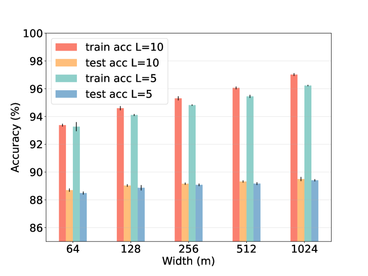
Figure 2: The accuracy of neural networks by NAS under different widths and depths.

F.4 Simulation of minimum eigenvalues of NTK

We calculate the minimum eigenvalue of each NTK matrix under different architectures with activation functions, skip connections and depths, according to Lemma 1. We consider four special cases on skip connections: a) no skip connections with $\bm{\alpha}=\bm{0}$, i.e., fully connected neural network in Figure 3(a); b) skip connections between all consecutive layers with $\bm{\alpha}=\bm{1}$, in Figure 3(b); c) the alpha of the first half (of the network) is $1$ and the alpha of the second half is $0$ shown in Figure 4(a); d) The alpha of the first half is $0$ and the alpha of the second half is $1$. The results are shown in Figure 4(b).

Figure 3(a) indicates that as the network depth increases, the minimum eigenvalue of NTK will become larger when LeakyReLU, ReLU, Swish and Tanh employed, but Sigmoid leads to a decreasing minimum eigenvalue, which is consistent with the upper bound shown in Theorem 1. The LeakyReLU, ReLU and Swish generate the fastest increasing rate of depth, while Tanh and Sigmoid are slow, which coincides with the derived lower bound in Theorem 1 and previous work Bietti and Bach [2021]. Figure 3(b) shows that, under the skip connection, the tendency of the minimum eigenvalue of NTK is similar to that of FC neural networks when various activation functions are employed. However, the specific values and the growth rate are significantly larger than FC neural networks. This result is consistent with the conclusion we state in Theorem 1 about skip layers leading to the increase of minimum eigenvalue of NTK with respect to the depth. Moreover, Figure 4 show similar growth speed.

Then, we plot the comparison figure of NTK under above two settings and two settings in main paper for the same activation function in Figure 5. In addition to reconfirming the order between different activation functions, we can also see that the effect of adding an activation layer in the second half of the $10$-layer neural network is better than the first half of the neural network. This verifies the experimental results in Figure 1(b).

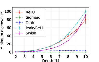
(a) no skip connections

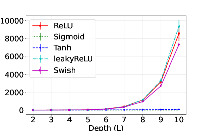
(b) skip connections

Figure 3: Minimum eigenvalue of NTK vs. depth ($L$) under various activation functions with/without skip connections in each layer.

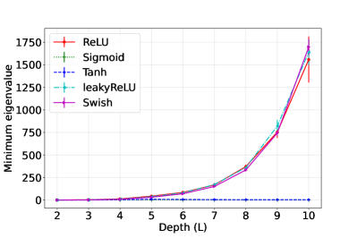
(a) the first half has a skip layer

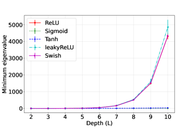
(b) the second half has a skip layer

Figure 4: Minimum eigenvalue of NTK vs. depth ($L$) under various activation functions with/without skip connections in each layer.

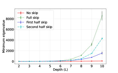
(a) ReLU

(b) LeakyReLU

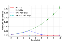
(c) Sigmoid

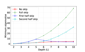
(d) Tanh

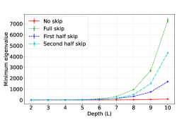
(e) Swish

Figure 5: Minimum eigenvalue of NTK for different activation function. The red line have skip connections in each layer, green line does not contain any skip connections, the blue line represents the skip connections in the first half and the cyan line represents the skip connections in the second half.

F.5 Additional experiments on NAS-Bench-101 and ranking correlations

In this section, we conduct more experiments on two new benchmarks NAS-Bench-101 [Ying et al., 2019] and Network Design Spaces (NDS) [Radosavovic et al., 2019] using the same setting as sec. 5.2.

Table 6 provides a comparison of the accuracy of Eigen-NAS, KNAS and NASWOT on four new search spaces. For all of four search spaces, our method achieves the best results with $1\%-2\%$ accuracy improvement.

Table 6: New results on NAS-Benchmark-101, NDS-DARTS and NDS-PNAS using CIFAR-10 and ImageNette2, a subset of ImageNet.

Benchmark	NAS-Bench-101	NDS-DARTS	NDS-PNAS	NDS-PNAS
Dataset	CIFAR-10	CIFAR-10	CIFAR-10	ImageNette2
Eigen-NAS ($k=20$)	$\bm{92.7\%}$	$\bm{92.6\%}$	$\bm{93.8\%}$	$\bm{69.2\%}$
KNAS ($k=20$)	$91.7\%$	$90.1\%$	$91.7\%$	$67.3\%$
NASWOT	$91.3\%$	$90.6\%$	$93.3\%$	$68.4\%$

Moreover, we conduct more detailed experiments using the CIFAR-10 dataset on NAS-Bench-101. Table 7 provides the running time and Kendall rank correlation coefficient between minimum eigenvalues and accuracy for the above three train-free NAS algorithm. We can see that our Eigen-NAS method can get the best rank correlation coefficient with the fastest speed among three methods. The scatter plot of the relationship between the minimum eigenvalue and the accuracy is shown in Figure 6.

Table 7: Running time (in Second) and the Kendall rank correlation coefficient on NAS-Bench-101, CIFAR-10 (the larger the absolute value of Rank correlation, the stronger the correlation between the guide used by the algorithm and the network accuracy).

Method	Eigen-NAS ($k=20$)	KNAS ($k=20$)	NASWOT
Running time	$\bm{1136}$	$1967$	$1468$
Rank correlation	$\bm{-0.355}$	$0.309$	$-0.313$

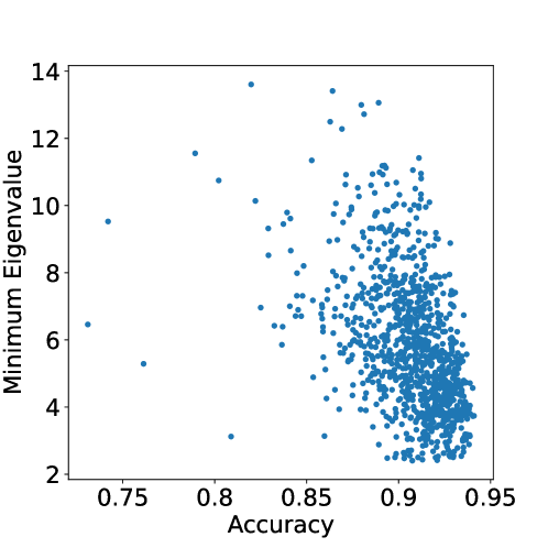
Figure 6: The standard scatter plot on the kendall rank correlation coefficient.

F.6 Transfer learning experiment

Here we evaluate the proposed NAS framework on transfer learning. The algorithm from sec. 5.1 is employed for this experiment, e.g., the same search space and search strategy. The experiment setting is the following: we train the model on FashionMNIST for $20$ epochs, then we use the pretrained weights and fine-tune them for $5$ epochs on MNIST, with repeated three times.

Table 8 show that, after the fine-tuning for just $2$ epochs, the method obtains up to $95\%$ accuracy and after fine-tuning for $5$ epochs it obtains up to $97\%$ accuracy. This verifies our intuition that the proposed NAS framework can obtain architectures that generalize well beyond the dataset they were optimized on.

Table 8: Transfer learning result of our network for different width ($m$) which training in FashionMNIST (domain dataset) for $20$ epochs and then training in MNIST (target dataset) for $2$ or $5$ epochs. (the accuracy in the table are displayed in percentages)

Epochs	$m=64$	$m=128$	$m=256$	$m=512$	$m=1024$
$20+2$	$94.13\pm 0.64$	$95.18\pm 0.25$	$94.73\pm 0.22$	$94.40\pm 0.80$	$\bm{95.41}\pm 0.03$
$20+5$	$95.73\pm 0.28$	$96.12\pm 0.32$	$96.73\pm 0.29$	$96.73\pm 0.11$	$\bm{96.96}\pm 0.22$

F.7 DARTS experiment on CNN

Our theory relies on fully-connected matrices and we have indeed verified experimentally the validity of our theoretical findings. To scrutinize our method even further, we attempt to extend our results to the popular convolutional neural networks. We believe this will provide some further insights on future extensions of our theory. In particular, we use DARTS (similarly with the experiment in sec. 5.1) with convolutional layers. The standard dataset of CIFAR-10 is selected; the details of the dataset are shared in sec. F.1. The search space and search strategy follow sec. 5.1 with one differentiating point: we use convolutional layers instead of fully connected layers in Equation 2.

We select DARTS on a Convolutional Neural Network with $L=10$ and $m=1024$, while we repeat the experiment for 5 times. After training, the probability of these activation functions and skip connections in each layer are reported in Figure 7(a) and 7(b), respectively. Compared with the Figure 1, the activation function search exhibits similar characteristics with the results of the fully connected network. Namely: (1) ReLU and LeakyReLU have the highest probability to be selected, (2) the difference of probability between different activation functions in the first layer is the largest. But for skip layer search, CNN exhibits the opposite results with fully connected network, that is, almost all of the skip connections have a probability of being selected less than $50\%$.

Based on the above results, our theory can still explain some of the phenomena observed in CNNs, e.g., activation functions search. Nevertheless, our theory on skip connections search on CNNs mismatches with experimental demonstration in practice to some extent, which motivates us to conduct a refined analysis on CNNs for NAS.

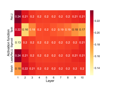
(a) activation functions $\bm{\sigma}$

(b) skip connections $\bm{\alpha}$

Figure 7: Architecture search results on activation functions indicated by the probability of $\bm{\sigma}$ in (a) and skip connections indicated by $\bm{\alpha}$ in (b). We notice that for each layer, ReLU and LeakyReLU are selected with the higher probability.

F.8 $\beta$-DARTS experiment on MLP

In this section, we use an improved DARTS-based algorithm, $\beta$-DARTS [Ye et al., 2022], for doing the activation function search. Our experiments are performed on a 5-layers MLP and the experimental results are presented in Figure 8. Compared with the results of DARTS in Figure 1, the experimental results of $\beta$-DARTS indicate that the probability difference between different activation functions is smaller, which may verify that DART is more easily to overfit . This is also the advantage mentioned in the $\beta$-DARTS paper.

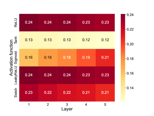
Figure 8: Architecture search results using $\beta$-DARTS on activation functions indicated by the probability of $\bm{\sigma}$. We notice that for each layer, ReLU and LeakyReLU are selected with the higher probability.

Appendix G Societal impact

This is a theoretical work that derived generalization bounds for the architectures obtained by NAS. As such, we do not expect our work to have negative societal bias, as we do not focus on obtaining state-of-the-art results in a particular task. On the contrary, our work can have various benefits for the community:

• We provide the first generalization bounds for the class of NAS architectures, which is expected to have a positive impact on the understanding and the application of such architectures.

• As we illustrate in sec. 5, we can use the minimum eigenvalue as a promising metric to guide NAS. This can lead to further investigation on techniques for efficient evaluation of NAS by avoiding solving the intensive bi-level optimization of NAS explicitly.

Nevertheless, we encourage researchers to further investigate the impact of different architectures and their inductive biases on the society.

References

- Allen-Zhu et al. (2018) Z. Allen-Zhu, Y. Li, and Y. Liang. Learning and generalization in overparameterized neural networks, going beyond two layers. In Advances in Neural Information Processing Systems (NeurIPS), 2018.
- Allen-Zhu et al. (2019) Z. Allen-Zhu, Y. Li, and Z. Song. A convergence theory for deep learning via over-parameterization. In International Conference on Machine Learning (ICML), 2019.
- Arora et al. (2019a) S. Arora, S. Du, W. Hu, Z. Li, and R. Wang. Fine-grained analysis of optimization and generalization for overparameterized two-layer neural networks. In International Conference on Machine Learning (ICML), 2019a.
- Arora et al. (2019b) S. Arora, S. S. Du, W. Hu, Z. Li, R. R. Salakhutdinov, and R. Wang. On exact computation with an infinitely wide neural net. In Advances in Neural Information Processing Systems (NeurIPS), 2019b.
- Bartlett et al. (2017) P. Bartlett, D. J. Foster, and M. Telgarsky. Spectrally-normalized margin bounds for neural networks. In Advances in Neural Information Processing Systems (NeurIPS), 2017.
- Belfer et al. (2021) Y. Belfer, A. Geifman, M. Galun, and R. Basri. Spectral analysis of the neural tangent kernel for deep residual networks, 2021.
- Bietti and Bach (2021) A. Bietti and F. Bach. Deep equals shallow for relu networks in kernel regimes. In International Conference on Learning Representations (ICLR), 2021.
- Cao and Gu (2019) Y. Cao and Q. Gu. Generalization bounds of stochastic gradient descent for wide and deep neural networks. In Advances in Neural Information Processing Systems (NeurIPS), 2019.
- Chen et al. (2021) W. Chen, X. Gong, and Z. Wang. Neural architecture search on imagenet in four gpu hours: A theoretically inspired perspective. In International Conference on Learning Representations (ICLR), 2021.
- Chen et al. (2019) Y. Chen, T. Yang, X. Zhang, G. Meng, X. Xiao, and J. Sun. Detnas: Backbone search for object detection. In Advances in Neural Information Processing Systems (NeurIPS), 2019.
- Chen et al. (2020a) Z. Chen, Y. Cao, Q. Gu, and T. Zhang. A generalized neural tangent kernel analysis for two-layer neural networks. In Advances in Neural Information Processing Systems (NeurIPS), 2020a.
- Chen et al. (2020b) Z. Chen, Y. Cao, D. Zou, and Q. Gu. How much over-parameterization is sufficient to learn deep ReLU networks? In International Conference on Learning Representations (ICLR), 2020b.
- Chrabaszcz et al. (2017) P. Chrabaszcz, I. Loshchilov, and F. Hutter. A downsampled variant of imagenet as an alternative to the cifar datasets, 2017.
- de Dios and Bruna (2020) J. de Dios and J. Bruna. On sparsity in overparametrised shallow relu networks, 2020.
- Deng et al. (2009) J. Deng, W. Dong, R. Socher, L.-J. Li, K. Li, and L. Fei-Fei. Imagenet: A large-scale hierarchical image database. In Conference on Computer Vision and Pattern Recognition (CVPR), 2009.
- Ding et al. (2020) S. Ding, T. Chen, X. Gong, W. Zha, and Z. Wang. Autospeech: Neural architecture search for speaker recognition, 2020.
- Dong and Yang (2020) X. Dong and Y. Yang. Nas-bench-201: Extending the scope of reproducible neural architecture search. In International Conference on Learning Representations (ICLR), 2020.
- Dong et al. (2021) X. Dong, L. Liu, K. Musial, and B. Gabrys. Nats-bench: Benchmarking nas algorithms for architecture topology and size. IEEE Transactions on Pattern Analysis and Machine Intelligence (T-PAMI), 2021.
- Du et al. (2019a) S. Du, J. Lee, H. Li, L. Wang, and X. Zhai. Gradient descent finds global minima of deep neural networks. In International Conference on Machine Learning (ICML), 2019a.
- Du et al. (2019b) S. S. Du, X. Zhai, B. Poczos, and A. Singh. Gradient descent provably optimizes over-parameterized neural networks. In International Conference on Learning Representations (ICLR), 2019b.
- Elsken et al. (2019) T. Elsken, J. H. Metzen, and F. Hutter. Neural architecture search: A survey. Journal of Machine Learning Research, 2019.
- Golub and Van Loan (1996) G. H. Golub and C. F. Van Loan. Matrix Computations (3rd Ed.). 1996.
- He et al. (2016) K. He, X. Zhang, S. Ren, and J. Sun. Deep residual learning for image recognition. In Conference on Computer Vision and Pattern Recognition (CVPR), 2016.
- Huang et al. (2020) K. Huang, Y. Wang, M. Tao, and T. Zhao. Why do deep residual networks generalize better than deep feedforward networks? – a neural tangent kernel perspective. In Advances in Neural Information Processing Systems (NeurIPS), 2020.
- Jacot et al. (2018) A. Jacot, F. Gabriel, and C. Hongler. Neural tangent kernel: Convergence and generalization in neural networks. In Advances in Neural Information Processing Systems (NeurIPS), 2018.
- Krizhevsky et al. (2014) A. Krizhevsky, V. Nair, and G. Hinton. The cifar-10 dataset. online: http://www. cs. toronto. edu/kriz/cifar. html, 2014.
- Lecun et al. (1998) Y. Lecun, L. Bottou, Y. Bengio, and P. Haffner. Gradient-based learning applied to document recognition. Proceedings of the IEEE, 1998.
- Li and Talwalkar (2020) L. Li and A. Talwalkar. Random search and reproducibility for neural architecture search. In Uncertainty in Artificial Intelligence, 2020.
- Liu et al. (2019a) C. Liu, L.-C. Chen, F. Schroff, H. Adam, W. Hua, A. L. Yuille, and L. Fei-Fei. Auto-deeplab: Hierarchical neural architecture search for semantic image segmentation. In Conference on Computer Vision and Pattern Recognition (CVPR), 2019a.
- Liu et al. (2018) H. Liu, K. Simonyan, O. Vinyals, C. Fernando, and K. Kavukcuoglu. Hierarchical representations for efficient architecture search. In International Conference on Learning Representations (ICLR), 2018.
- Liu et al. (2019b) H. Liu, K. Simonyan, and Y. Yang. Darts: Differentiable architecture search. In International Conference on Learning Representations (ICLR), 2019b.
- Malach et al. (2020) E. Malach, G. Yehudai, S. Shalev-Schwartz, and O. Shamir. Proving the lottery ticket hypothesis: Pruning is all you need. In International Conference on Machine Learning (ICML), 2020.
- Mellor et al. (2021) J. Mellor, J. Turner, A. Storkey, and E. J. Crowley. Neural architecture search without training. In International Conference on Machine Learning (ICML), 2021.
- Montanari and Zhong (2020) A. Montanari and Y. Zhong. The interpolation phase transition in neural networks: Memorization and generalization under lazy training, 2020.
- Nguyen (2021) Q. Nguyen. On the proof of global convergence of gradient descent for deep relu networks with linear widths. In International Conference on Machine Learning (ICML), 2021.
- Nguyen et al. (2021) Q. Nguyen, M. Mondelli, and G. F. Montufar. Tight bounds on the smallest eigenvalue of the neural tangent kernel for deep relu networks. In International Conference on Machine Learning (ICML), 2021.
- Nguyen and Mondelli (2020) Q. N. Nguyen and M. Mondelli. Global convergence of deep networks with one wide layer followed by pyramidal topology. In Advances in Neural Information Processing Systems (NeurIPS), 2020.
- Oymak and Soltanolkotabi (2020) S. Oymak and M. Soltanolkotabi. Toward moderate overparameterization: Global convergence guarantees for training shallow neural networks. IEEE Journal on Selected Areas in Information Theory, 2020.
- Oymak et al. (2021) S. Oymak, M. Li, and M. Soltanolkotabi. Generalization guarantees for neural architecture search with train-validation split. In International Conference on Machine Learning (ICML), 2021.
- Radosavovic et al. (2019) I. Radosavovic, J. Johnson, S. Xie, W.-Y. Lo, and P. Dollár. On network design spaces for visual recognition. In International Conference on Computer Vision (ICCV), 2019.
- Ren et al. (2021) P. Ren, Y. Xiao, X. Chang, P.-Y. Huang, Z. Li, X. Chen, and X. Wang. A comprehensive survey of neural architecture search: Challenges and solutions. ACM Computing Surveys (CSUR), 2021.
- Schur (1911) J. Schur. Bemerkungen zur theorie der beschränkten bilinearformen mit unendlich vielen veränderlichen. Journal für die reine und angewandte Mathematik, 1911.
- Shu et al. (2020) Y. Shu, W. Wang, and S. Cai. Understanding architectures learnt by cell-based neural architecture search. In International Conference on Learning Representations (ICLR), 2020.
- Shu et al. (2022) Y. Shu, S. Cai, Z. Dai, B. C. Ooi, and B. K. H. Low. NASI: Label- and data-agnostic neural architecture search at initialization. In International Conference on Learning Representations (ICLR), 2022.
- Tan and Le (2019) M. Tan and Q. Le. Efficientnet: Rethinking model scaling for convolutional neural networks. In International Conference on Machine Learning (ICML), 2019.
- Tirer et al. (2022) T. Tirer, J. Bruna, and R. Giryes. Kernel-based smoothness analysis of residual networks. In Mathematical and Scientific Machine Learning, 2022.
- Vershynin (2018) R. Vershynin. High-Dimensional Probability: An Introduction with Applications in Data Science. 2018.
- Wu et al. (2019) B. Wu, X. Dai, P. Zhang, Y. Wang, F. Sun, Y. Wu, Y. Tian, P. Vajda, Y. Jia, and K. Keutzer. Fbnet: Hardware-aware efficient convnet design via differentiable neural architecture search. In Conference on Computer Vision and Pattern Recognition (CVPR), 2019.
- Xiao et al. (2017) H. Xiao, K. Rasul, and R. Vollgraf. Fashion-mnist: a novel image dataset for benchmarking machine learning algorithms, 2017.
- Xu et al. (2021) J. Xu, L. Zhao, J. Lin, R. Gao, X. Sun, and H. Yang. Knas: Green neural architecture search. In International Conference on Machine Learning (ICML), 2021.
- Xu et al. (2019) Y. Xu, L. Xie, X. Zhang, X. Chen, G.-J. Qi, Q. Tian, and H. Xiong. Pc-darts: Partial channel connections for memory-efficient architecture search. In International Conference on Learning Representations (ICLR), 2019.
- Yaskov (2014) P. Yaskov. Lower bounds on the smallest eigenvalue of a sample covariance matrix. Electronic Communications in Probability, 2014.
- Ye et al. (2022) P. Ye, B. Li, Y. Li, T. Chen, J. Fan, and W. Ouyang. -darts: Beta-decay regularization for differentiable architecture search. In Conference on Computer Vision and Pattern Recognition (CVPR), 2022.
- Ying et al. (2019) C. Ying, A. Klein, E. Christiansen, E. Real, K. Murphy, and F. Hutter. Nas-bench-101: Towards reproducible neural architecture search. In International Conference on Machine Learning (ICML), 2019.
- Zhang et al. (2019) Y. Zhang, Z. Qiu, J. Liu, T. Yao, D. Liu, and T. Mei. Customizable architecture search for semantic segmentation. In Conference on Computer Vision and Pattern Recognition (CVPR), 2019.
- Zhou et al. (2020) P. Zhou, C. Xiong, R. Socher, and S. C. Hoi. Theory-inspired path-regularized differential network architecture search. In Advances in Neural Information Processing Systems (NeurIPS), 2020.
- Zoph and Le (2017) B. Zoph and Q. V. Le. Neural architecture search with reinforcement learning. In International Conference on Learning Representations (ICLR), 2017.
- Zoph et al. (2018) B. Zoph, V. Vasudevan, J. Shlens, and Q. V. Le. Learning transferable architectures for scalable image recognition. In Conference on Computer Vision and Pattern Recognition (CVPR), 2018.
- Zou et al. (2019) D. Zou, Y. Cao, D. Zhou, and Q. Gu. Gradient descent optimizes over-parameterized deep relu networks. Machine Learning, 2019.