Recovery Guarantees for Distributed-OMP

Abstract

We study distributed schemes for high-dimensional sparse linear regression, based on orthogonal matching pursuit (OMP). Such schemes are particularly suited for settings where a central fusion center is connected to end machines, that have both computation and communication limitations. We prove that under suitable assumptions, distributed-OMP schemes recover the support of the regression vector with communication per machine linear in its sparsity and logarithmic in the dimension. Remarkably, this holds even at low signal-to-noise-ratios, where individual machines are unable to detect the support. Our simulations show that distributed-OMP schemes are competitive with more computationally intensive methods, and in some cases even outperform them.

1 INTRODUCTION

Sparse linear regression is a fundamental problem in machine learning, statistics and signal processing. Indeed, sparsity is a natural and widely applied modeling assumption in high dimensional settings. A sparsity assumption gives rise to the variable selection problem, of identifying a small subset of variables which are most informative for a given prediction problem. We consider the popular sparse linear regression model with random noise,

$$y=\mathbf{x}^{\top}\bm{\theta}+\sigma\xi,$$ (1)

where $y\in\mathbb{R}$ is the response, $\mathbf{x}\in\mathbb{R}^{d}$ is a vector of explanatory variables, $\bm{\theta}\in\mathbb{R}^{d}$ is the unknown vector of regression coefficients, $\xi\in\mathbb{R}$ is a standard normal random variable, i.e., $\xi\sim\mathcal{N}\left(0,1\right)$, and $\sigma>0$ is the noise level. We consider a high dimensional setting $d\gg 1$ with a vector $\bm{\theta}$ of sparsity $K=\left\lVert\bm{\theta}\right\rVert_{0}\ll d$. In a centralized setting, given $N$ samples from (1), common tasks are to accurately estimate $\bm{\theta}$ as well as its support $\mathcal{S}=\mbox{supp}(\bm{\theta})=\{i\mid\theta_{i}\neq 0\}$. Many methods have been proposed and analyzed to solve these tasks, including combinatorial algorithms, linear programming, greedy approaches and regularization schemes (Mallat and Zhang, 1993; Tibshirani, 1996; Chen et al., 2001; Miller, 2002; Candes and Tao, 2005; Tropp and Gilbert, 2007; Blumensath and Davies, 2008; Needell and Tropp, 2009; Dai and Milenkovic, 2009; Bertsimas et al., 2016; Hastie et al., 2020; Amir et al., 2021).

In various contemporary applications, the data is stored across multiple machines. Moreover, due to communication or privacy constraints, the data at each machine cannot be sent to other machines in the network. Such cases bring about various distributed learning problems, see Wimalajeewa and Varshney (2017); Jordan et al. (2019) and references therein.

A common distributed setting, which we also consider here, consists of $M$ machines connected in a star topology to a fusion center, with each machine having for simplicity an equal number of samples, $n=N/M$. For the sparse model (1), some distributed methods attempt to recover the centralized solution that would have been computed by the fusion center, if it had access to all $N=nM$ samples of the $M$ machines. Examples include optimization-based methods (Mateos et al., 2010; Ling and Tian, 2011; Ling et al., 2012; Fosson et al., 2016; Mota et al., 2011), Bayesian approaches (Makhzani and Valaee, 2013; Khanna and Murthy, 2016), and greedy schemes (Sundman et al., 2012; Li et al., 2015; Patterson et al., 2014; Han et al., 2015; Chouvardas et al., 2015). These methods are in general communication intensive, as they are iterative and may require many rounds to converge. A simpler single round divide-and-conquer scheme, is for each machine to send its own estimate of $\bm{\theta}$ and for the fusion center to average these estimates. For a wide range of problems, the resulting estimator has a risk comparable to that of the centralized solution (Rosenblatt and Nadler, 2016; Wang et al., 2017; Jordan et al., 2019; Liu et al., 2023). For the sparse linear regression model (1), Lee et al. (2017) and Battey et al. (2018) proposed a single round distributed debiased-Lasso scheme, and proved that under suitable conditions it achieves the same error rate as the centralized solution. Yet, these debiased-Lasso methods have two limitations: (i) the communication per machine is at least linear in $d$; and (ii) the computational costs are considerable, as each machine has to solve $d+1$ Lasso problems. Barghi et al. (2021) and Fonseca and Nadler (2023) proposed debiased-Lasso methods with much less communication, where each machine sends to the center only the indices of its few largest coordinates.

We consider distributed estimation of the sparse vector $\bm{\theta}$ in the model (1), under the following setting: The $M$ end machines have both limited processing power and a restricted communication budget. This is motivated by modern applications where end machines are computationally weak, but collect high dimensional data. For example, in spectrum sensing, a network of sensors continuously monitor and collect high dimensional data, and repeatedly need to estimate the current vector $\bm{\theta}$. In these settings, computationally intensive methods such as debiased Lasso may be infeasible or prohibitively slow. In addition, regardless of computational considerations, most of the above methods are not applicable in high dimensions, as their communication per machine is at least linear in $d$.

As the quantity of interest $\bm{\theta}$ is $K$-sparse with $K\ll d$, this gives rise to the following challenge: develop a scheme that accurately estimates the vector $\bm{\theta}$ with number of operations per machine linear in $d$ and communication sublinear in $d$, and derive theoretical guarantees for it. Here we focus on accurately estimating the support of $\bm{\theta}$. Indeed, as discussed in Battey et al. (2018); Fonseca and Nadler (2023), given an accurate estimate of the support, an additional single round of communication allows distributed estimation of $\bm{\theta}$ with the same error rate as in the centralized setting.

A natural base algorithm for machines with low computational resources is Orthogonal Matching Pursuit (OMP), as it is one of the fastest methods for sparse recovery (Chen et al., 1989; Pati et al., 1993; Mallat and Zhang, 1993). Several distributed-OMP schemes to estimate the support of $\bm{\theta}$, which are computationally fast and incur little communication, were proposed in Duarte et al. (2005); Wimalajeewa and Varshney (2013); Sundman et al. (2014). In terms of theory, to the best of our knowledge, the only work to derive support recovery guarantees for distributed-OMP methods is Wimalajeewa and Varshney (2014). However, their analysis is restricted to a noise-less compressed-sensing setting, with samples $\mathbf{x}_{i}$ that are random and independent across machines. Their proof is based on an underlying symmetry between all non-support variables. In contrast, we consider a more general setting with deterministic samples corrupted by additive noise, for which their proof technique is not applicable.

Our key contribution is the derivation of a recovery guarantee for a distributed-OMP scheme, see Theorem 4.1. Remarkably, our guarantee holds even at low signal-to-noise ratios (SNRs), where each individual machine fails to recover the support. The main challenge in our analysis is that the samples $\mathbf{x}_{i}$, assumed deterministic, may be similar (or even identical) across machines. Hence, at low signal-to-noise ratios, several machines might send the same incorrect support variable to the fusion center. Deriving a theoretical guarantee in this case requires a different and more delicate analysis than that of previous works. Specifically, to bound the probability that a non-support variable is sent to the fusion center we use recent lower bounds on the maximum of correlated Gaussian random variables (Lopes and Yao, 2022). Our analysis provides insight how distributed-OMP methods can achieve exact support recovery even at low SNR where individual machines fail to do so.

To complement our theoretical analysis, in Section 5 we compare via simulations the support-recovery success of several algorithms including distributed-OMP, debiased Lasso schemes (Lee et al., 2017; Battey et al., 2018; Barghi et al., 2021), and distributed variants of sure independence screening (SIS) (Fan and Lv, 2008), which are also suitable for computationally weak machines. In a distributed variant of SIS, each machine first excludes variables weakly correlated to the response, and then estimates the sparse vector $\bm{\theta}$ on the remaining ones via any appropriate algorithm. In our experiments we considered smoothly clipped absolute deviation (SCAD) (Fan and Li, 2001) and OMP. As expected, our simulations show that the best performing scheme is debiased Lasso, but at the expense of significantly higher communication and computational costs. Interestingly, in comparison to a communication-restricted thresholded variant of debiased Lasso, distributed-OMP methods perform comparably, and in some cases even outperform it, while being orders of magnitude faster. Furthermore, applying SIS followed by OMP at each machine performed in some cases even slightly better that distributed-OMP. We conclude the paper with a discussion in Section 6.

Notation

We use the standard $O(\cdot),\Omega(\cdot),\Theta(\cdot)$ notation to hide constants independent of the problem parameters and $\tilde{O}(\cdot)$ to hide terms polylogarithmic in $d$. For functions $f,g$, the notations $f=o(g)$ and $f\ll g$ mean that $f(d)/g(d)\to 0$ as $d\to\infty$. We say that an estimator $\hat{S}$ achieves exact support recovery with high probability if $\Pr\left[\hat{S}=\mathcal{S}\right]\to 1$ as both $d\to\infty$ and the number of machines $M=M(d)\to\infty$ at a suitable rate. The smallest integer larger than or equal to $x$ is denoted $\lceil x\rceil$. For a standard Gaussian $Z\sim\mathcal{N}(0,1)$, the complement of its cumulative distribution function is $\Phi^{c}(t)=\Pr[Z>t]$. We denote the inner product of two vectors ${\mathbf{u}},{\mathbf{v}}$ by $\langle{\mathbf{u}},{\mathbf{v}}\rangle={\mathbf{u}}^{\top}{\mathbf{v}}$.

2 PROBLEM SETUP

We consider linear regression with a sparse coefficient vector in a distributed setting, where $M$ machines are connected in a star topology to a fusion center. Each machine $m\in[M]$ holds $n$ samples from the sparse regression model (1), i.e., a design matrix $\mathbf{X}^{(m)}\in\mathbb{R}^{n\times d}$ and a response vector $\mathbf{y}^{(m)}\in\mathbb{R}^{n}$, related via

$$\mathbf{y}^{(m)}=\mathbf{X}^{(m)}\bm{\theta}+\sigma\bm{\xi}^{(m)},$$ (2)

where $\bm{\xi}^{(m)}\sim\mathcal{N}\left(0,\mathbf{I}_{n}\right)$ and $\sigma$ is the unknown noise level. While the $M$ machines may have the same or similar design matrices, their noises $\bm{\xi}^{(m)}$ are assumed to be independent. We assume $\bm{\theta}$ is $K$-sparse, namely $\left\lVert\bm{\theta}\right\rVert_{0}=\left|\operatorname{supp}(\bm{\theta})\right|=K$, with the value of $K$ known to the center.

The problem we consider is exact recovery of the support of $\bm{\theta}$, which is a standard goal in sparse linear regression, and has been widely studied in both non-distributed and distributed settings. We study this problem under the constraints that the $M$ machines have limited computational resources and limited communication with the fusion center. This setting is relevant in various applications including distributed compressed sensing and sensor networks.

3 DISTRIBUTED OMP SCHEMES

OMP-based schemes are popular for sparse support recovery, and are highly attractive in distributed settings where computation and communication are limited. We consider two distributed OMP schemes to estimate the support of $\bm{\theta}$. Both schemes use the following subroutine, denoted OMP_Step, which performs a single step of the OMP algorithm, and outputs a new variable to be added to the current support set. As outlined in Algorithm 1, given a matrix $\mathbf{X}$, a vector $\mathbf{y}$, and a support set $S$, the subroutine computes $\hat{\bm{\theta}}$, the least squares approximation of $\bm{\theta}$ on the support $S$ and its residual vector $\mathbf{r}$. It then outputs an index $j\in[d]$ whose column $\mathbf{x}_{j}$ has maximal correlation with $\mathbf{r}$. A key property of OMP_Step is the orthogonality of the residual to the columns of $\mathbf{X}$ in the set $S$. Hence, the output of OMP_Step is a new index $j\notin S$.

The simplest distributed OMP method is for each machine to separately run OMP for $K$ steps and send its $K$ locally-computed indices to the fusion center. The center estimates the support of $\bm{\theta}$ by the $K$ indices that received the largest number of votes. To cope with low-SNR regimes where the top $K$ indices at individual machines may not include all support indices, we propose a variant where each machine runs OMP for a larger number of steps and thus sends a support of size $L>K$. This scheme, which we call Distributed OMP (D-OMP), is outlined in Algorithm 2.

1

input  :  $\mathbf{X}\in\mathbb{R}^{n\times d}$, $\mathbf{y}\in\mathbb{R}^{n}$, support set $S$

output : support index $j$

2 compute $\hat{\bm{\theta}}=\mbox{argmin}_{\mathbf{z}\in\mathbb{R}^{d},\operatorname{supp}(\mathbf{z})=S}\left\|\mathbf{y}-\mathbf{X}\mathbf{z}\right\|_{2}$

3 compute residual $\mathbf{r}=\mathbf{y}-\mathbf{X}\hat{\bm{\theta}}$

4 output index $j=\arg\max\left\{\frac{\lvert\langle\mathbf{x}_{i},\mathbf{r}\rangle\rvert}{\left\lVert\mathbf{x}_{i}\right\rVert}:i\in[d]\right\}$

5

Algorithm 1 OMP_Step

1

2At each machine $m=1,\dots,M$ 

       input :  $\mathbf{X}^{(m)}\in\mathbb{R}^{n\times d}$, $\mathbf{y}^{(m)}\in\mathbb{R}^{n}$, integer $L$

       output : message $S^{(m)}_{L}$ to center

3       initialize $S^{(m)}_{0}=\emptyset$

4       for round $t=1,\dots,L$ do

5             $j^{(m,t)}=\texttt{OMP\_Step}\left(\mathbf{X}^{(m)},\mathbf{y}^{(m)},S^{(m)}_{t-1}\right)$

6             update support set $S^{(m)}_{t}=S^{(m)}_{t-1}\cup\left\{j^{(m,t)}\right\}$

7       end for

8      send $S^{(m)}_{L}$ to the center

9

10At the fusion center 

       input : messages $\left\{S^{(m)}_{L}\right\}_{m\in[M]}$, sparsity $K$

       output : estimated support $S$

11       for each index $j\in\left[d\right]$, calculate the number of votes it received $\mathbf{v}_{j}=\sum_{m\in[M]}\mathbb{1}\left\{j\in S^{(m)}_{L}\right\}$

12       sort indices by number of votes, $\mathbf{v}_{\pi(1)}\geq\dots\geq\mathbf{v}_{\pi(d)}$

13       return $K$ indices with most votes $S=\left\{\pi(1),\dots,\pi(K)\right\}$

14      

15

Algorithm 2 Distributed OMP (D-OMP)

1

2initialize $S_{0}=\emptyset$

3

4for round $t=1,\dots,K$ do

5       At each machine $m=1,\dots,M$ 

6             $j^{(m,t)}=\texttt{OMP\_Step}\left(\mathbf{X}^{(m)},\mathbf{y}^{(m)},S_{t-1}\right)$

7            send index $j^{(m,t)}$ to fusion center

8      

9      At the fusion center 

             input : messages $j^{(m,t)}$, sparsity $K$

10             calculate number of votes for each index $j$, $\mathbf{v}^{(t)}_{j}=\sum_{m\in[M]}\mathbb{1}\left\{j=j^{(m,t)}\right\}$

11             find most voted index $j_{t}=\mbox{argmax}_{j}\mathbf{v}^{(t)}_{j}$

12             add $j_{t}$ to support set $S_{t}=S_{t-1}\cup\{j_{t}\}$

13             send $j_{t}$ to all machines

14             if $t=K$ output $S_{K}$

15      

16      

17 end for

Algorithm 3 Distributed Joint OMP

A second scheme, which we call Distributed Joint OMP (DJ-OMP), computes the support set one index at a time, using $K$ communication rounds. Starting with an empty support set $S_{0}=\emptyset$, at each round $t=1,\dots,K$, the center sends the current set $S_{t-1}$ to the $M$ machines. Then, each machine calls OMP_Step and sends the resulting index $j^{(m,t)}$ to the center. At the end of each round, the center adds to the support set an index $j_{t}$ that received the most votes, $S_{t}=S_{t-1}\cup\{j_{t}\}$. After $K$ rounds, the center outputs the support set $S_{K}$. Since OMP_Step outputs an index not in the current set $S_{t-1}$, at each round $t$ of DJ-OMP, a new index is indeed added by the center, $j_{t}\notin S_{t-1}$. This scheme is outlined in Algorithm 3.

Computation and Communication Complexity.

Let us first analyze the number of operations in a single execution of OMP_Step. Given a support set $S$, computing $\hat{\bm{\theta}}$ via least squares involves multiplying a $\left|S\right|\times n$ matrix by its transpose, and then inverting the resulting $\left|S\right|\times\left|S\right|$ matrix. Next, finding the index $j$ most correlated to the residual requires $d$ inner products of vectors in $\mathbb{R}^{n}$. For $\left|S\right|$ sufficiently small, say $o\left(d^{1/3}\right)$, the computational cost of OMP_Step is dominated by the latter step whose cost is $O(nd)$.

We now compare the two schemes DJ-OMP and D-OMP with $L=K$. In terms of computational complexity, in both schemes each machine performs the same number of operations. Thus, for $K=o\left(d^{1/3}\right)$ their computational complexity per machine is $O(ndK)$. In terms of communication, in both schemes each machine sends and receives a total of $K$ indices, and so the communication per machine is $O(K\log d)$ bits. The main difference is that D-OMP performs a single round, whereas DJ-OMP performs $K$ rounds. Hence, DJ-OMP requires synchronization and is slower in comparison to D-OMP.

Related Works.

Various distributed-OMP methods were proposed in the past decade. Wimalajeewa and Varshney (2013) considered the same D-OMP scheme as we do, with $L=K$. In addition, they proposed a DC-OMP algorithm, which is similar to DJ-OMP. In DC-OMP, at each round, instead of adding just one index to the support, the fusion center adds all indices that received at least two votes. A distributed-OMP approach for a different setting where each machine has its own regression vector $\bm{\theta}^{(m)}$ was proposed in Sundman et al. (2014). In their setting, the support sets of the $M$ vectors $\bm{\theta}^{(m)}$ are assumed to be similar, and the $M$ machines are connected in a general topology without a fusion center.

4 THEORETICAL RESULTS

Despite their simplicity, to the best of our knowledge, distributed-OMP schemes lack rigorous mathematical support and only limited theoretical results have been derived for them. Wimalajeewa and Varshney (2014) proved a support recovery guarantee for DC-OMP, but only in a restricted noise-less compressed-sensing setting, where the entries of the design matrices are all random and i.i.d. across machines. In contrast, in this section we derive a support recovery guarantee for DJ-OMP, under a more general setting, where the design matrices are deterministic and potentially structured, and the responses $y$ are noisy. Specifically, we prove in Theorem 4.1 that if the SNR is large enough (the non-zero entries of $\bm{\theta}$ are sufficiently large in absolute value), then with high probability DJ-OMP recovers the support set $\mathcal{S}$. Remarkably, the SNR required by our theorem is well below that required for individual machines to succeed. Its proof appears in Appendix A.

Towards stating our result formally, we first recall recovery guarantees for OMP on a single machine, and mathematically define the SNR in our problem.

Distributed Coherence Condition.

The coherence of a matrix $\mathbf{A}$ with columns $\mathbf{a}_{j}$ is defined as

$$\mu\left(\mathbf{A}\right)=\max_{i\neq j}\frac{\left|\left\langle\mathbf{a}_{i},\mathbf{a}_{j}\right\rangle\right|}{\left\lVert\mathbf{a}_{i}\right\rVert_{2}\left\lVert\mathbf{a}_{j}\right\rVert_{2}}.$$ (3)

A matrix $\mathbf{A}$ satisfies the Mutual Incoherence Property (MIP) with respect to a sparsity level $K$ if

$$\mu(\mathbf{A})<\frac{1}{2K-1}.$$ (4)

A fundamental result by Tropp (2004) is that in an ideal noise-less setting ($\sigma=0$), the MIP condition (4) is sufficient for exact support recovery by OMP.

In our distributed setting, each machine $m$ has its own design matrix $\mathbf{X}^{(m)}$ with coherence $\mu^{(m)}=\mu(\mathbf{X}^{(m)})$. We denote their maximal coherence by

$$\mu_{\max}=\mu_{\max}(\mathbf{X}^{(1)},\dots,\mathbf{X}^{(M)})=\max_{m\in[M]}\mu^{(m)}.$$ (5)

We say that a set of matrices $\mathbf{X}^{(1)},\dots,\mathbf{X}^{(M)}$ satisfies the max-MIP condition w.r.t. a sparsity level $K$ if

$$\mu_{\max}<\frac{1}{2K-1}.$$ (6)

Eq. (6) implies that all machines satisfy the MIP condition (4). Hence, in a noise-less setting, OMP at each machine will correctly recover the support of $\bm{\theta}$. The coherence plays a key role for OMP recovery also in the presence of noise, as we discuss next.

SNR Regime.

We formally define the SNR in our distributed setting. We then focus on an interesting regime, in which the SNR is sufficiently high for OMP to recover the support of $\bm{\theta}$ in a centralized setting, where the center has access to all the samples from all machines, and yet too low for OMP at a single machine to individually recover it. For a $K$-sparse vector $\bm{\theta}\in\mathbb{R}^{d}$, a matrix $\mathbf{A}\in\mathbb{R}^{n\times d}$ with coherence $\mu$ whose columns have unit norm, and a noise level $\sigma$, define

$$\theta_{{\mbox{\tiny crit}}}(\mu,d,K,\sigma)=\frac{\sigma\sqrt{2\log d}}{1-(2K-1)\mu}.$$ (7)

Notice it is well defined under the MIP condition (4).

As in previous works, to derive exact support recovery guarantees, we consider vectors $\bm{\theta}$ whose non-zero entries have magnitude lower bounded by $\theta_{\min}$, namely $\min_{k\in\mathcal{S}}\left|\theta_{k}\right|\geq\theta_{\min}$. For a matrix $\mathbf{A}$ with unit-norm columns, define the SNR as $r=\left(\frac{\theta_{\min}}{\theta_{{\mbox{\tiny crit}}}(\mu,d,K,\sigma)}\right)^{2}$. Near the value $r=1$, OMP (at a single machine) exhibits a phase transition from failure to success of support recovery. If the SNR is slightly higher, i.e., $r>\left(1+\sqrt{\frac{\log K}{\log d}}\right)^{2}$, then with high probability OMP exactly recovers the support $\mathcal{S}$ (Ben-Haim et al., 2010). In contrast, if the SNR is slightly lower, i.e., $r<\left(1-\sqrt{\frac{\log K}{\log d}}-\mu\right)^{2}$, then there are matrices $\mathbf{A}\in\mathbb{R}^{n\times d}$ with coherence $\mu$ and $K$-sparse vectors $\bm{\theta}\in\mathbb{R}^{d}$ for which given $\mathbf{y}=\mathbf{A}\bm{\theta}+\sigma\bm{\xi}$, OMP fails with high probability to recover the support of $\bm{\theta}$. In addition, this occurs empirically for several common families of matrices $\mathbf{A}$ and vectors $\bm{\theta}$ (Amiraz et al., 2021).

In our distributed setting the matrices $\mathbf{X}^{(m)}$ are assumed to be deterministic and do not necessarily have unit-norm columns. However, (2) is equivalent to

$$\mathbf{y}^{(m)}=\tilde{\mathbf{X}}^{(m)}\tilde{\bm{\theta}}^{(m)}+\sigma\bm{\xi}^{(m)},$$ (8)

where each column $\tilde{\mathbf{x}}_{j}^{(m)}$ of the matrix $\tilde{\mathbf{X}}^{(m)}$ is scaled to have unit norm, i.e., $\tilde{\mathbf{x}}_{j}^{(m)}={\mathbf{x}_{j}^{(m)}}/\|\mathbf{x}_{j}^{(m)}\|$, and accordingly $\tilde{\theta}_{j}^{(m)}=\|\mathbf{x}_{j}^{(m)}\|\theta_{j}$. Clearly, the support of each $\tilde{\bm{\theta}}^{(m)}$ is identical to that of $\bm{\theta}$. We assume that for a suitable $\tilde{\theta}_{\min}$, the vector $\bm{\theta}$ satisfies that

$$\min_{m}\|\mathbf{x}_{k}^{(m)}\|\left|\theta_{k}\right|\geq\tilde{\theta}_{\min},\quad\forall k\in\mathcal{S}.$$ (9)

Given the above discussion, in our distributed setting we define the SNR parameter $r$ as follows,

$$r=\left(\frac{\tilde{\theta}_{\min}}{\theta_{{\mbox{\tiny crit}}}(\mu_{\max},d,K,\sigma)}\right)^{2}.$$ (10)

If $r>1$ then $\tilde{\theta}_{\min}>\theta_{{\mbox{\tiny crit}}}(\mu^{(m)},d,K,\sigma)$ at every machine $m\in[M]$, and hence OMP in any single machine would recover the support of $\bm{\theta}$ with high probability.

Next, consider a centralized setting where all $N=Mn$ samples are available to the fusion center. This setting corresponds to a response vector $\mathbf{y}\in\mathbb{R}^{N}$ and measurement matrix $\mathbf{X}\in\mathbb{R}^{N\times d}$ formed by column-stacking $\mathbf{y}^{(1)},\dots,\mathbf{y}^{(M)}$ and $\mathbf{X}^{(1)},\dots,\mathbf{X}^{(M)}$, respectively. In analogy to (10), to guarantee support recovery in this case, a sufficient condition is that the centralized SNR $r^{(c)}=\left(\frac{\tilde{\theta}_{\min}^{(c)}}{\theta_{{\mbox{\tiny crit}}}(\mu(\mathbf{X}),d,K,\sigma)}\right)^{2}>1$. Here $\tilde{\theta}_{\min}^{(c)}$ is a value such that for all support indices $k\in\mathcal{S}$, $|\theta_{k}|\geq\tilde{\theta}_{\min}^{(c)}/\|\mathbf{X}_{k}\|$, where $\mathbf{X}_{k}$ is the $k$-th column of $\mathbf{X}$. Since $\left\lVert\mathbf{X}_{k}\right\rVert\geq\sqrt{M}\min_{m}\left\lVert\mathbf{x}_{k}^{(m)}\right\rVert$, then in a centralized setting OMP is guaranteed to succeed when $\sqrt{M}\tilde{\theta}_{\min}>\theta_{{\mbox{\tiny crit}}}(\mu(\mathbf{X}),d,K,\sigma)$. Given the definition (7) for $\theta_{{\mbox{\tiny crit}}}$, an SNR regime that is interesting to study in the distributed setting is

$$\frac{1}{M}\left(\frac{1-(2K-1)\mu_{\max}}{1-(2K-1)\mu(\mathbf{X})}\right)^{2}<r<1.$$ (11)

As we show next, for a subrange of the SNR values in Eq. (11), the DJ-OMP scheme can still achieve exact support recovery.

4.1 Support Recovery Guarantee

We present three assumptions for our recovery guarantee to hold. As OMP is based on dot products between the residual and normalized columns of the design matrices, we first introduce the following quantity that bounds how large these can be,

$$\delta=\delta\left(K,\mu_{\max}\right)=\tfrac{\left(K-1\right)\mu_{\max}^{2}}{1-\left(K-2\right)\mu_{\max}}.$$ (12)

As we show in Section A.5, under the max-MIP condition (6), $\delta\leq\mu_{\max}$. Our first assumption is that the number of machines is sufficiently large, with the dependence on $K$ encoded in the quantity $\delta$.

Assumption 4.1.

$M\geq M_{c}\left(d,K,\mu_{\max},r\right)$, where

$$M_{c}\left(d,K,\mu_{\max},r\right)=K\left\lceil\frac{16\log d}{\Phi^{c}\left(\tfrac{(1-\sqrt{r})\sqrt{2\log d}}{\sqrt{1-\delta}(1-\mu_{\max})}\right)}\right\rceil.$$ (13)

In our analysis, we assume that $d\gg 1$ and that $\mu_{\max}$ is small. This implies that also $\delta$ is small and hence

$$M_{c}\left(d,K,\mu_{\max},r\right)\approx Kd^{\left(\frac{1-\sqrt{r}}{\sqrt{1-\delta}(1-\mu_{\max})}\right)^{2}},$$ (14)

which follows from the approximation $\Phi^{c}(t)\approx e^{-t^{2}/2}$ and omitting $O(\log d)$ factors. Thus, larger SNR values (though still smaller than one), require fewer machines to guarantee support recovery.

To guarantee support recovery by DJ-OMP, we also need to upper bound the probability that a non-support index is sent to the fusion center. As described in the appendix, for this we use a recent result on the left tail of the maximum of correlated Gaussian random variables (Lopes and Yao, 2022). The SNR that guarantees recovery thus depends on a parameter $\epsilon=\epsilon(K,\mu_{\max})$, with smaller values of $\epsilon$ leading to a lower SNR. However, for our proof to work, $\epsilon$ cannot be arbitrarily small, and we set it as follows.

Assumption 4.2.

The scalar $\epsilon=\epsilon(K,\mu_{\max})$ satisfies

$$\frac{\sqrt{\mu_{\max}+\delta}}{1+\sqrt{\mu_{\max}+\delta}}<\epsilon<1.$$ (15)

Importantly, for $\mu_{\max}$ small, $\epsilon$ can be chosen to be as small as $O(\sqrt{\mu_{\max}})$. As detailed in the theorem below, this allows recovery at low SNRs.

Finally, we define a few quantities that characterize the lower bound we impose on the SNR $r$. Let

$$Q_{0}\left(d,K\right)=\tfrac{\log\left(88\sqrt{2}K\right)}{\log d},$$ (16)

and define $Q_{1}\left(d,K,\mu_{\max},\epsilon\right)$ and $Q_{2}\left(d,K,\mu_{\max}\right)$ by

$$Q_{1}=\tfrac{1-\left(1-\mu_{\max}\right)\sqrt{1-\delta}\left(\left(1-\epsilon\right)\sqrt{1-\mu_{\max}}-\sqrt{Q_{0}}\right)}{1-2\mu_{\max}K\sqrt{1-\delta}\frac{1-\mu_{\max}}{1-\left(2K-1\right)\mu_{\max}}},$$ (17)

$$Q_{2}=\tfrac{\sqrt{2+2\left(\mu_{\max}+\delta\right)}\left(1+\sqrt{1-\delta}\left(1-\mu_{\max}\right)\sqrt{Q_{0}}\right)}{\sqrt{1-\delta}\left(1-\mu_{\max}\right)+\sqrt{2+2\left(\mu_{\max}+\delta\right)}}.$$ (18)

Assumption 4.3 (SNR Condition).

The SNR $r$ is lower bounded as follows

$$\sqrt{r}\geq\left\{\begin{array}[]{ll}Q_{2}&(4K-1)\mu_{\max}-2K\mu_{\max}^{2}\geq 1\\ \min(Q_{1},Q_{2})&\mbox{\rm otherwise}\end{array}\right.$$ (19)

We can now state our support recovery guarantee. The following theorem shows that under the above assumptions, the DJ-OMP algorithm, which indeed requires lightweight communication and computation, recovers the support of $\bm{\theta}$, with high probability.

Theorem 4.1.

Under Assumptions 4.1-4.3 and the max-MIP condition (6), for sufficiently large $d=d(\epsilon)$, with probability at least $1-2^{K+1}/d,$ DJ-OMP with $K$ rounds recovers the support of the $K$-sparse vector $\bm{\theta}$.

Let us analyze the implications of the theorem when $K\ll d$ and $\mu_{\max},\epsilon,\delta\ll 1$. In this case $Q_{1}\approx\epsilon$ and $Q_{2}\approx\frac{\sqrt{2}}{1+\sqrt{2}}$. Hence, Assumption 4.3 is approximately $r>(\min(Q_{1},Q_{2}))^{2}\approx\epsilon^{2}$ or $r\gtrsim\mu_{\max}$. Thus, there is a range of relatively low SNR values for which with a sufficiently large number of machines, DJ-OMP is guaranteed to recover the support, even though individual machines fail to do so.

Remark 4.1.

Several works considered distributed settings where each machine has a different vector $\bm{\theta}^{(m)}$, but they are all share the same support $\mathcal{S}$ (Duarte et al., 2005; Ling and Tian, 2011; Ling et al., 2012; Wimalajeewa and Varshney, 2014; Li et al., 2015). Theorem 4.1 also holds in such cases, under the following condition on the vectors $\bm{\theta}^{(m)}$, instead of (9),

$$\min_{m\in[M]}\left\lVert\mathbf{x}_{k}^{(m)}\right\rVert\left|\theta_{k}^{(m)}\right|\geq\tilde{\theta}_{\min}\quad\forall k\in\mathcal{S}.$$

We now compare Theorem 4.1 to related works. Amiraz et al. (2022) studied distributed sparse mean estimation, which is a special case of distributed sparse linear regression where the design matrices are orthogonal. They designed low-communication distributed schemes that provably recover the support for a wide range of SNR values. However, their proofs rely on the design matrices being orthogonal, and do not generalize to incoherent matrices. Their schemes are single-round, essentially using the orthogonality to recover all $K$ support indices in parallel, in contrast to our DJ-OMP scheme which has $K$ iterations, and requires a careful analysis of error propagation. As mentioned above, Wimalajeewa and Varshney (2014) considered a compressed-sensing setting with incoherent random matrices whose entries are drawn i.i.d. from the same distribution, and with no noise ($\sigma=0$). In both of these papers, a key property that greatly simplifies the analysis is that at all machines the probability for selecting a non-support index is the same for all $k\notin\mathcal{S}$. Our theorem shows that even without this symmetry between the non-support indices, distributed-OMP algorithms can achieve exact support recovery.

5 SIMULATION RESULTS

We compare experimentally the following algorithms, which have different computation and communication costs (see Table 1): (i) Deb-Lasso where each machine computes a debiased-Lasso estimate of $\bm{\theta}\in\mathbb{R}^{d}$ and sends it to the center. The center averages these $M$ vectors and returns its top $K$ indices (Lee et al., 2017; Battey et al., 2018); (ii) Deb-Lasso-K, a variant of Barghi et al. (2021), where each machine sends the top $K$ indices of its debiased-Lasso estimate; (iii) SIS-SCAD-K, a distributed variant SIS, where each machine performs variable screening followed by SCAD (Fan and Lv, 2008). It sends its resulting support set to the center, which selects the top $K$ indices by majority voting; (iv) SIS-OMP-K, another distributed variant of SIS. Here, each machine estimates its support set using OMP on the remaining features; (v) D-OMP with $L=K$; (vi) D-OMP with $L=2K$; and (vii) DJ-OMP. To illustrate the ability of DJ-OMP to recover the support when individual machines fail, for reference we also ran OMP on a single machine, ignoring the data in all other $M-1$ machines. Note that while OMP-based schemes are essentially parameter free (beyond the sparsity $K$), the debiased-Lasso schemes required knowledge of the noise level $\sigma$ in all machines.

Table 1: Communication and Computation Costs

Algorithm	Communication cost	Computational cost, $K\ll d^{1/3}$
Single OMP	$\tilde{O}\left(K\right)$	$O\left(ndK\right)$
Deb-Lasso	$\tilde{O}\left(d\right)$	solving $d+1$ Lasso optimization problems
Deb-Lasso-K	$\tilde{O}\left(K\right)$
SIS-SCAD-K	SNR dependent	$O\left(nd\right)$
SIS-OMP-K	$\tilde{O}\left(K\right)$
D-OMP, $L\!=\!K$	$\tilde{O}\left(K\right)$	$O\left(ndK\right)$
DJ-OMP

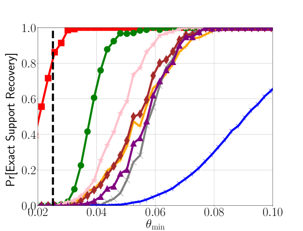
(a) IID Design Matrices ($\alpha=0$)

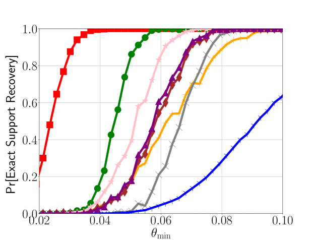
(b) Correlated Design Matrices ($\alpha=0.1$)

Figure 1: Support Recovery as a Function of $\theta_{\min}$.

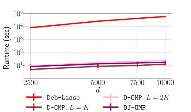
Figure 2: Runtime as a Function of $d$.

We now describe the experimental setup. Each matrix $X^{(m)}$ is generated as follows. Each row is drawn independently from $\mathcal{N}(\mathbf{0},\Sigma)$, where $\Sigma$ is a Toeplitz matrix with $\Sigma_{ii}=1$ and $\Sigma_{ij}=\alpha^{\left|i-j\right|}$ for $i\neq j$ for some $\alpha\in[0,1)$. In all settings, we generate $M=20$ such matrices, each containing $n=2000$ samples. The noise level is $\sigma=1$, and the vector $\bm{\theta}$ has a sparsity $K=5$, with $\bm{\theta}=\theta_{\min}\cdot[1,-1.5,2,-2.5,3,0,\dots,0]^{\top}$. The tuning parameter in the debiased-Lasso methods, which scales the $\ell_{1}$ term of each of the $d+1$ Lasso objectives, is set to $\lambda=2\sigma\sqrt{\frac{\log d}{n}}$. We consider two settings both of dimension $d=10000$. In Setting (a), $\alpha=0$, i.e., all matrix entries are i.i.d. $\mathcal{N}(0,1)$. In Setting (b), $\alpha=0.1$, so the columns of $X^{(m)}$ are weakly correlated. Further implementation details appear in Appendix C.

Figure 1 illustrates the empirical success probability of the various algorithms as a function of $\theta_{\min}$ in the two settings outlined above. Formally, for an algorithm $A$,

$$p_{\text{ success }}^{A}(\theta_{\min})=\frac{1}{J}\sum_{j=1}^{J}\mathbb{1}\left\{S_{j}^{A}(\theta_{\min})=\mathcal{S}\right\},$$

where $S_{j}^{A}(\theta_{\min})$ is the support set computed by algorithm $A$, for noise realization $j$ and lower bound $\theta_{\min}$ on the non-zero coefficients of $\bm{\theta}$, and $J$ is the total number of noise realizations, set to $J=500$. The dashed vertical line in panel (a) is the lower bound $\theta_{{\mbox{\tiny crit}}}(\mu(\mathbf{X}),d,K,\sigma)$ of Eq. (7), above which in a centralized setting, OMP is guaranteed to recover the support. In panel (b), the MIP condition does not hold and the dashed line is not shown. Nonetheless, distributed schemes still succeed in this case.

Figure 1 reveals several behaviors. First, as anticipated, the distributed-OMP algorithms perform inferior to Deb-Lasso, which incurs much higher computational and communication costs. Second, in accordance with Theorem 4.1, the distributed-OMP algorithms succeed at low SNR values, where OMP on a single machine fails with high probability. Third, DJ-OMP’s performance is comparable to D-OMP with $L=K$. For scenarios requiring one-shot communication, D-OMP with more steps, $L=2K$ in this example, exceeds DJ-OMP’s performance, while incurring a slightly higher communication cost. In Setting (a) where each entry of the matrices $\mathbf{X}^{(m)}$ is i.i.d. Gaussian, the performance of distributed-OMP algorithms is on par with the computationally demanding Deb-Lasso-K. Notably, in Setting (b) where the matrices $\mathbf{X}^{(m)}$ have correlated columns, distributed-OMP methods surpass Deb-Lasso-K. In the context of variable screening methods, for a wide range of SNR values, a single machine often misses the full support set during the screening step. Yet, incorporating voting schemes enables distributed support recovery. Similar to Deb-Lasso-K, SIS-SCAD-K matches the performance of distributed-OMP algorithms in Setting (a) but lags behind them in Setting (b). In all the studied settings, SIS-OMP-K consistently outperforms both SIS-SCAD-K and DJ-OMP. A theoretical study of this behavior is an interesting topic for future research.

Figure 2 shows the runtime and error bars of several schemes, all implemented in Python, as a function of $d$ on a logarithmic scale. In this simulation, $\alpha=0$ and $\theta_{\min}=0.1$ and we averaged over $J=20$ realizations. The runtime of Deb-Lasso-K is similar to that of Deb-Lasso, and thus not shown. As seen in the figure, distributed-OMP methods are more than three orders of magnitude faster than Deb-Lasso. Not shown are the runtimes SIS-based schemes, which are slower than DJ-OMP, but are not directly comparable since for them we called from Python an existing R code.

Finally, in Appendix B we show empirically that the number of machines to recover the support scales as $M\approx d^{\beta}$ for some $\beta<1$, in accordance with (14).

6 DISCUSSION

Distributed inference schemes can be assessed based on three criteria: (i) the SNR above which they succeed with high probability; (ii) the communication per machine; and (iii) the computational requirements. Figure 3 illustrates how distributed-OMP schemes compare with other methods for sparse linear regression. Each scheme is represented by a circle, whose size encodes the computational cost per machine (on a logarithmic scale). The $x$-axis is the SNR and the $y$-axis is the communication per machine.

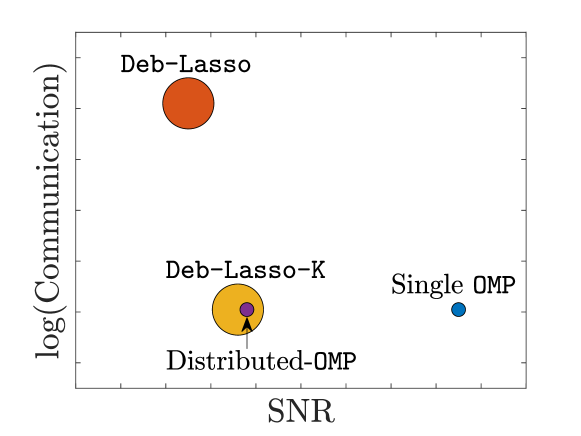
Figure 3: SNR, Communication and Computation Tradeoffs.

As seen in the figure, known schemes exhibit a tradeoff between SNR and communication. When the SNR is sufficiently high for an individual machine to recover the support of $\bm{\theta}$, for example by OMP, the fusion center may recover the support $\mathcal{S}$ by contacting only one machine, incurring an incoming communication of only $O(K\log d)$ bits. Note that even in a noise-less setting, for the fusion center to recover the support, $K$ indices must be sent to the center, so $K\log d$ bits is a lower bound on the total required communication. On the other hand, when the SNR is low, Deb-Lasso succeeds to recover the support of $\bm{\theta}$ but incurs a communication cost of $\tilde{O}\left(d\right)$ bits per machine, which might be prohibitive in high-dimensional settings.

We conjecture that at low-SNR values, no distributed algorithm can achieve exact support recovery with communication per machine $O(K\log d)$ bits. We note that for closely related problems, achieving the centralized minimax $\ell_{2}$ risk or the centralized prediction error is possible at low SNR but requires communication cost of $\Omega(d)$ bits (Shamir, 2014; Steinhardt and Duchi, 2015; Acharya et al., 2019). Our work shows that for a range of SNR values between these two extremes, distributed-OMP algorithms do recover the support of $\bm{\theta}$ with communication per machine $O(K\log d)$. An interesting open question is to determine the optimal rate at which the required communication decreases as a function of the SNR by any distributed algorithm that achieves exact support recovery. Another interesting direction for future research is to characterize the tradeoff between communication costs and computational resources.

Appendix A PROOFS

In this section we prove Theorem 4.1. For ease of presentation, in Section A.1 we state and prove Theorem A.1 which addresses the simpler case $K=1$. The proof of Theorem 4.1 for the general case $K\geq 1$ appears in Section A.2. The proofs of various auxiliary lemmas appear in Sections A.3-A.6.

Towards proving both theorems, we first present a few preliminaries, state useful lemmas and outline the proof.

Preliminaries.

Recall that DJ-OMP is an iterative algorithm, whereby at each round $t$, all $M$ machines call the subroutine OMP_Step with the same input set $S_{t-1}$. In principle, except at the first round where $S_{0}=\emptyset$, this input set depends on all the data in all $M$ machines. This statistical dependency significantly complicates the analysis. Instead, as discussed below, in our proof we will analyze a single round of DJ-OMP, assuming all machines are provided with a fixed input set $s$.

Given an input set $s$ to the subroutine OMP_Step, each machine $m$ computes a sparse vector supported on $s$, i.e.,

$$\hat{\bm{\theta}}^{(m)}=\arg\min_{\mathbf{z}\in\mathbb{R}^{d}}\left\|\mathbf{y}^{(m)}-\mathbf{X}^{(m)}\mathbf{z}\right\|_{2}\text{ s.t. }\operatorname{supp}(\mathbf{z})=s.$$ (20)

Then, it calculates the corresponding residual vector

$$\mathbf{r}^{(m)}=\mathbf{y}^{(m)}-\mathbf{X}^{(m)}\hat{\bm{\theta}}^{(m)}.$$ (21)

Finally, each machine $m$ sends to the fusion center the index

$$j^{(m)}=\arg\max_{i\in[d]}\lvert\langle\tilde{\mathbf{x}}^{(m)}_{i},\mathbf{r}^{(m)}\rangle\rvert,$$ (22)

where $\tilde{\mathbf{x}}^{(m)}_{i}=\frac{\mathbf{x}^{(m)}_{i}}{\left\lVert\mathbf{x}^{(m)}_{i}\right\rVert}$ is the $i$-th column of $\mathbf{X}^{(m)}$ divided by its norm.

As also described in Algorithm 3, given the messages sent by all $M$ machines, the fusion center computes a vector $\mathbf{v}\in\mathbb{R}^{d}$, where $\mathbf{v}_{j}$ counts the number of votes received by index $j$ for all $j\in[d]$. As discussed in the main text, indices in $s$ receive no votes and at each round a new index $j_{\text{center}}$ is chosen by the center,

$$j_{\text{center}}=j_{\text{center}}\left(s\right)=\arg\max_{j\in[d]\setminus s}\mathbf{v}_{j}.$$

Towards proving that with high probability $j_{\text{center}}\in\mathcal{S}\setminus s$, we define an additional quantity $\rho^{(m)}=\rho^{(m)}(s)$ that corresponds to the local SNR at machine $m$ given an input set $s$. Denote

$$\tilde{\theta}_{\max}^{(m)}=\tilde{\theta}_{\max}^{(m)}(s)=\max_{k\in\mathcal{S}\setminus s}\left\{\left\lVert\mathbf{x}_{k}^{(m)}\right\rVert\left|\theta_{k}\right|\right\}.$$ (23)

Similar to the definition of $r$ in Eq. (10), we define

$$\rho^{(m)}=\rho^{(m)}(s)=\left(\frac{\tilde{\theta}_{\max}^{(m)}}{\theta_{{\mbox{\tiny crit}}}\left(\mu_{\max},d,K,\sigma\right)}\right)^{2},$$ (24)

where $\theta_{{\mbox{\tiny crit}}}$ is defined in Eq. (7). Where clear from the context and to simplify notation we will not write the dependence on the input set $s$ explicitly. Note that by its definition, for any input set $s$ that is strictly contained in $\mathcal{S}$, it follows that $\rho^{(m)}\geq r$. As discussed in Section 4, if $\rho^{(m)}>1$, then with high probability machine $m$ would recover a support index, namely $j^{(m)}\in\mathcal{S}\setminus s$ (Amiraz et al., 2021). Therefore, in what follows, we consider a worst case scenario whereby $\rho^{(m)}\leq 1$ in all machines $m\in[M]$.

Proof outline and lemmas.

For simplicity we prove the theorem assuming the number of machines is the smallest that still satisfies Assumption 4.1, namely $M=M_{c}\left(d,K,\mu_{\max},r\right)$, with $M_{c}$ defined in Eq. (13). A larger number of machines would only increase the probability of exact support recovery. The main idea of the proof is to show that at each of the $K$ rounds, with high probability the center indeed chooses a support index. Specifically, consider a single round of DJ-OMP with a fixed input set $s\subset\mathcal{S}$. Then, for the center to choose an index $j_{\text{center}}\in\mathcal{S}\setminus s$, it suffices that there exists some support index $k\in\mathcal{S}\setminus s$ that received more votes than any non-support index, namely,

$$\mathbf{v}_{k}>\max_{j\notin\mathcal{S}}\mathbf{v}_{j}.$$ (25)

A sufficient condition for (25) to occur is that for some suitable threshold $t_{c}=t_{c}(s)>0$, both

$$\mathbf{v}_{k}>t_{c},$$ (26)

and

$$\max_{j\notin\mathcal{S}}\mathbf{v}_{j}<t_{c}.$$ (27)

As described below, our chosen threshold $t_{c}$ depends on the following quantity $F$, which provides a lower bound for the probability that a support index is sent to the center by one of the machines,

$$F\left(d,K,\mu_{\max},r\right)=\frac{1}{2}\Phi^{c}\left(\tfrac{(1-\sqrt{r})\sqrt{2\log d}}{\sqrt{1-\delta}(1-\mu_{\max})}\right).$$ (28)

Note that by this definition, Eq. (13) can be rewritten as

$$M_{c}\left(d,K,\mu_{\max},r\right)=K\left\lceil\frac{8\log d}{F\left(d,K,\mu_{\max},r\right)}\right\rceil.$$ (29)

We will show that Eqs. (26) and (27) indeed hold with high probability with the following threshold

$$t_{c}=t_{c}(s)=\frac{\sum_{m\in[M]}F\left(d,K,\mu_{\max},\rho^{(m)}(s)\right)}{M\cdot F\left(d,K,\mu_{\max},r\right)}4\log d,$$ (30)

where $r$, $\rho^{(m)}$ and $F$ are defined in Eqs. (10), (24), and (28) respectively. Note that $\rho^{(1)},\dots,\rho^{(M)}$ and $t_{c}$, which all depend also on the subset $s$, are not assumed to be known to the center and are only used in the proof.

The following Lemma A.1 provides a lower bound for the threshold $t_{c}$, which will be useful in our proofs. Its proof follows directly from the definition of $F$ in Eq. (28) and appears in Section A.3.

Lemma A.1.

Under the max-MIP condition (6), for any fixed $s\subset\mathcal{S}$, the threshold $t_{c}=t_{c}(s)$ defined in Eq. (30) satisfies

$$t_{c}\geq 4\log d.$$ (31)

The following Lemma A.2 states that if the expected number of votes for an index $k\in\mathcal{S}\setminus s$ is sufficiently high, then event (26) occurs with high probability. The next Lemma A.3 shows that if the expected number of votes for each non-support index $j\notin\mathcal{S}$ is sufficiently low, then event (27) occurs with high probability. These lemmas follow from Chernoff bounds and are proved in Section A.3 as well.

Lemma A.2.

Assume the max-MIP condition (6) holds. Fix $s\subset\mathcal{S}$, and let $t_{c}=t_{c}(s)$ be given by Eq. (30). If $\textup{E}\left[\mathbf{v}_{k}\right]\geq 2t_{c}$ for some $k\in\mathcal{S}\setminus s$, then

$$\Pr\left[\mathbf{v}_{k}\leq t_{c}\right]\leq\frac{1}{d}.$$

Lemma A.3.

Assume the max-MIP condition (6) holds. Fix $s\subset\mathcal{S}$, and let $t_{c}=t_{c}(s)$ be given by Eq. (30). If for all non-support indices $j\notin\mathcal{S}$ it holds that $\textup{E}\left[\mathbf{v}_{j}\right]\leq\frac{t_{c}}{5}$ then

$$\Pr\left[\max_{j\notin\mathcal{S}}\mathbf{v}_{j}\geq t_{c}\right]\leq\frac{1}{d}.$$

It remains to bound $\textup{E}\left[\mathbf{v}_{j}\right]$ from above for $j\in\mathcal{S}\setminus s$ and from below for $j\notin\mathcal{S}$. Towards this goal, denote by $p^{(m)}_{j}$ the probability that machine $m$ sends index $j$, namely

$$p^{(m)}_{j}=\Pr\left[j^{(m)}=j\right],$$ (32)

where $j^{(m)}$ is defined in Eq. (22).

Since $\textup{E}\left[\mathbf{v}_{j}\right]=\sum_{m}p_{j}^{(m)}$, it suffices to bound the probability $p_{j}^{(m)}$. For ease of presentation, we first derive these bounds for the case $K=1$ in Section A.1, and then extend them to the general case $K\geq 1$ in Section A.2.

A.1 Support recovery guarantee for sparsity $K=1$

For completeness, we rewrite Assumptions 4.1-4.3 for this case. Since $K=1$, by its definition in Eq. (12), $\delta\left(1,\mu_{\max}\right)=0$. Hence, the quantity $F$ simplifies to

$$F\left(d,1,\mu_{\max},r\right)=\frac{1}{2}\Phi^{c}\left(\frac{1-\sqrt{r}}{1-\mu_{\max}}\sqrt{2\log d}\right),$$ (33)

and the quantity $M_{c}$ from Eq. (29) reduces to

$$M_{c}\left(d,1,\mu_{\max},r\right)=\left\lceil\frac{8\log d}{F\left(d,1,\mu_{\max},r\right)}\right\rceil.$$ (34)

Thus, for $K=1$, Assumptions 4.1 and 4.2 read as follows:

Assumption A.1.

$M\geq M_{c}\left(d,1,\mu_{\max},r\right)$.

Assumption A.2.

The parameter $\epsilon=\epsilon(\mu_{\max})$ satisfies

$$\frac{\sqrt{\mu_{\max}}}{1+\sqrt{\mu_{\max}}}<\epsilon<1.$$ (35)

The quantity $Q_{0}$ reduces to

$$Q_{0}\left(d,1\right)=\frac{\log\left(88\sqrt{2}\right)}{\log d}.$$ (36)

In addition, the expressions for $Q_{1}$ and $Q_{2}$ simplify to

$$Q_{1}\left(d,1,\mu_{\max},\epsilon\right)=\frac{1-\left(1-\mu_{\max}\right)\left(\left(1-\epsilon\right)\sqrt{1-\mu_{\max}}-\sqrt{Q_{0}}\right)}{1-2\mu_{\max}},$$ (37)

$$Q_{2}\left(d,1,\mu_{\max}\right)=\frac{\sqrt{2+2\mu_{\max}}\left(1+\left(1-\mu_{\max}\right)\sqrt{Q_{0}}\right)}{1-\mu_{\max}+\sqrt{2+2\mu_{\max}}}.$$ (38)

Finally, for $K=1$, Assumption 4.3 on the SNR is:

Assumption A.3 (SNR Condition).

The SNR is sufficiently high,

$$\sqrt{r}\geq\left\{\begin{array}[]{ll}Q_{2}&\mu_{\max}\geq 1/2\\ \min(Q_{1},Q_{2})&\mbox{otherwise}\end{array}\right.$$ (39)

Theorem A.1.

Under Assumptions A.1-A.3 and the max-MIP condition $\mu_{\max}<1$, for sufficiently large $d=d(\epsilon)$, with probability at least $1-2/d,$ a single round of DJ-OMP recovers the support of a $1$-sparse vector $\bm{\theta}$.

A few remarks are in place. First, note that when $K=1$, D-OMP with $L=1$ reduces to the same algorithm as DJ-OMP, and thus this result holds for this algorithm as well. Second, as mentioned in Section 4, when $\mu_{\max}\ll 1$ condition (39) roughly translates to $r\gtrsim\epsilon^{2}$, and hence $r\gtrsim\mu_{\max}$. Thus, there is a range of relatively low SNR values for which DJ-OMP succeeds to recover the support, even though the probability of any single machine to do so is very low.

A.1.1 Proof of Theorem A.1

When $K=1$, only a single round is performed with an input set $s=\emptyset$. Thus it trivially holds that $s\subset\mathcal{S}$. In addition, OMP_Step simplifies to the following procedure. At each contacted machine $m$, the residual is simply the response vector, i.e., $\mathbf{r}^{(m)}=\mathbf{y}^{(m)}$. Thus, the index sent by machine $m$ to the fusion center is given by

$$j^{(m)}=\arg\max_{i\in[d]}\lvert\langle\tilde{\mathbf{x}}^{(m)}_{i},\mathbf{y}^{(m)}\rangle\rvert.$$ (40)

Another simplification in the case $K=1$ is that the support set contains only one index, which we denote by $k$, i.e., $\mathcal{S}=\left\{k\right\}$. To prove Theorem A.1, we derive a lower bound on the probability $p_{k}^{(m)}$ for the support index $k$ in the following Lemma A.4 and an upper bound on the probability $p_{j}^{(m)}$ for each non-support index $j\notin\mathcal{S}$ in the following Lemma A.5. Their proofs appear in Section A.4 and are based on a probabilistic analysis of the inner products between the response vector $\mathbf{y}^{(m)}$, which consists of signal and noise, and different columns $\tilde{\mathbf{x}}_{i}$.

Lemma A.4.

Assume that $\left\|\bm{\theta}\right\|_{0}=K=1$ and let $\mathcal{S}=\left\{k\right\}=\operatorname{supp}\left\{\bm{\theta}\right\}$. Further assume that the max-MIP condition (6) holds. For sufficiently large $d$, for each machine $m$,

$$p_{k}^{(m)}\geq F\left(d,1,\mu_{\max},\rho^{(m)}\right),$$ (41)

where $p_{k}^{(m)}$ and $F$ are defined in Eqs. (32) and (33) respectively.

Lemma A.5.

Assume that $\left\|\bm{\theta}\right\|_{0}=K=1$ and let $\mathcal{S}=\operatorname{supp}\left\{\bm{\theta}\right\}$. Further assume that $\rho^{(m)}$ of Eq. (24) satisfies $\rho^{(m)}\leq 1$ for each machine $m$ and that the max-MIP condition (6) holds. If $\epsilon$ satisfies Assumption A.2, the SNR parameter $r$ satisfies Assumption A.3, and the dimension $d=d(\epsilon)$ is sufficiently large, then for each machine $m$ and each non-support index $j\notin\mathcal{S}$,

$$p_{j}^{(m)}\leq\frac{F\left(d,1,\mu_{\max},\rho^{(m)}\right)}{11}.$$ (42)

We now formally prove Theorem A.1 by combining the above lemmas.

Proof of Theorem A.1.

For simplicity, we assume that the number of machines is $M=M_{c}\left(d,1,\mu_{\max},r\right)$, since a larger number of machines would only increase the probability of successful support recovery. We first analyze the probability that event (26) occurs. By Lemma A.4, for the support index $k\in\mathcal{S}$, its expected number of votes is $\textup{E}\left[\mathbf{v}_{k}\right]=\sum_{m\in[M]}p_{k}^{(m)}\geq\sum_{m\in[M]}F\left(d,1,\mu_{\max},\rho^{(m)}\right)$. By the definitions of $t_{c}$ in Eq. (30) and $M_{c}$ in Eq. (34),

$$\textup{E}\left[\mathbf{v}_{k}\right]\geq\frac{M_{c}\cdot F\left(d,1,\mu_{\max},r\right)}{4\log d}\cdot t_{c}=\left\lceil\frac{8\log d}{F\left(d,1,\mu_{\max},r\right)}\right\rceil\frac{F\left(d,1,\mu_{\max},r\right)}{4\log d}\cdot t_{c}\geq 2t_{c}.$$

By Lemma A.2, the event (26) occurs with probability at least $1-1/d$.

Next, we analyze the probability that event (27) occurs. Fix a non-support index $j\notin\mathcal{S}$. Since $\rho^{(m)}\leq 1$, then by Lemma A.5, its expected number of votes is $\textup{E}\left[\mathbf{v}_{j}\right]=\sum_{m\in[M]}p_{j}^{(m)}\leq\frac{1}{11}\sum_{m\in[M]}F\left(d,1,\mu_{\max},\rho^{(m)}\right)$. By the definitions of $t_{c}$ in Eq. (30) and $M_{c}$ in Eq. (34),

$$\textup{E}\left[\mathbf{v}_{j}\right]\leq\frac{1}{11}\left\lceil\frac{8\log d}{F\left(d,1,\mu_{\max},r\right)}\right\rceil\frac{F\left(d,1,\mu_{\max},r\right)}{4\log d}t_{c}<\frac{t_{c}}{5}.$$

The last inequality is justified as follows. Recall that $\lceil x\rceil\leq x+1$ for all $x$. Thus,

$$\left\lceil\frac{8\log d}{F\left(d,1,\mu_{\max},r\right)}\right\rceil\frac{F\left(d,1,\mu_{\max},r\right)}{4\log d}\leq 2+\frac{F\left(d,1,\mu_{\max},r\right)}{4\log d}.$$

By the definition of $F$ in Eq. (33), it follows that $F\left(d,1,\mu_{\max},r\right)\leq 1$. Hence, when $d\geq 8$, then $\log d>2$, and the term $\frac{F\left(d,1,\mu_{\max},r\right)}{4\log d}\leq\frac{1}{8}$. Hence, by Lemma A.3, the event (27) occurs with probability at least $1-1/d$. A union bound completes the proof. ∎

A.2 Proof of Theorem 4.1

We now prove that with high probability, DJ-OMP succeeds to recover the support of $\bm{\theta}$ with general sparsity level $K$. The proof relies on the following lemma, which bounds the probability that, given a fixed input set $s$, the center chooses an incorrect index at a single round of the algorithm.

Lemma A.6.

Let $s\subset[d]$ be a fixed set of indices given as input to a single round of DJ-OMP and denote by $j_{\text{center}}\left(s\right)$ the index chosen by the center at the end of this round. Under Assumptions 4.1-4.3 and the max-MIP condition (6), for sufficiently large $d=d(\epsilon)$, if $s\subset\mathcal{S}$ then the index $j_{\text{center}}\left(s\right)$ also belongs to the support set $\mathcal{S}$ with high probability. Specifically,

$$\Pr\left[j_{\text{center}}\left(s\right)\notin\mathcal{S}\right]\leq 2d^{-1}.$$ (43)

First, let us show how Theorem 4.1 follows directly from Lemma A.6.

Proof of Theorem 4.1.

Recall that DJ-OMP starts with $S_{0}=\emptyset$, adds exactly one new index to the estimated support set at each round, and runs for exactly $K$ rounds. We denote by $S_{1},S_{2},\ldots,S_{K}$ the index sets found by the center after $t=1,2,\ldots,K$ distributed rounds of DJ-OMP, respectively.

Our goal is to upper bound the probability that $S_{K}$, the output of DJ-OMP after $K$ rounds, is not the true support set $\mathcal{S}$. To this end we decompose this failure probability according to the round at which the failure occurred,

$$\Pr\left[S_{K}\neq\mathcal{S}\right]=\sum_{t=1}^{K}\sum_{\overset{s_{t-1}\subset\mathcal{S}}{|s_{t-1}|=t-1}}\Pr\left[j_{t}\left(s_{t-1}\right)\notin\mathcal{S}\text{ and }S_{t-1}=s_{t-1}\right].$$

Directly analyzing each of the terms above is challenging due to the statistical dependency between the set of indices found so far $S_{t-1}$, and the new index found in the current round. To overcome this, we use the inequality $\Pr[A\cap B]\leq\Pr[A]$, which gives

$$\Pr\left[S_{K}\neq\mathcal{S}\right]\leq\sum_{t=1}^{K}\sum_{\overset{s_{t-1}\subset\mathcal{S}}{|s_{t-1}|=t-1}}\Pr\left[j_{t}(s_{t-1})\notin\mathcal{S}\right].$$

Since now the set $s_{t-1}$ is fixed, we can bound each term via Lemma A.6. This gives

$$\Pr\left[S_{K}\neq\mathcal{S}\right]\leq\frac{2}{d}\sum_{t=1}^{K}{K\choose t-1}=\frac{2}{d}\left(2^{K}-1\right)\leq\frac{2^{K+1}}{d},$$

which completes the proof. ∎

Next, we prove Lemma A.6. Since $s\subset\mathcal{S}$, we need to bound the probability $p_{j}^{(m)}$ of Eq. (32) for $j\in\mathcal{S}\setminus s$ and for $j\notin\mathcal{S}$. We shall do so using the following two lemmas. The first one, Lemma A.7, lower bounds a different quantity $q^{(m)}$ defined as the probability that the index sent by machine $m$ belongs to the support $\mathcal{S}\setminus s$,

$$q^{(m)}=q^{(m)}(s)=\Pr\left[j^{(m)}\in\mathcal{S}\setminus s\right].$$ (44)

Lemma A.8 upper bounds $p_{j}^{(m)}$ for each $j\notin\mathcal{S}$. Their proofs appear in Section A.5.

Lemma A.7.

Assume that the max-MIP condition (6) holds. For each machine $m$, for sufficiently large $d$,

$$q^{(m)}\geq F\left(d,K,\mu_{\max},\rho^{(m)}\right),$$ (45)

where $q^{(m)}$ and $F$ are defined in Eqs. (44) and (28) respectively.

Lemma A.8.

Assume that $\rho^{(m)}$ of Eq. (24) satisfies $\rho^{(m)}\leq 1$ for each machine $m$ and that the max-MIP condition (6) holds. If $\epsilon$ satisfies Assumption 4.2, the SNR parameter $r$ satisfies Assumption 4.3, and the dimension $d=d(\epsilon)$ is sufficiently large, then for each machine $m$ and each non-support index $j\notin\mathcal{S}$,

$$p_{j}^{(m)}\leq\frac{F\left(d,K,\mu_{\max},\rho^{(m)}\right)}{11K},$$ (46)

where $p_{j}^{(m)}$ and $F$ are defined in Eqs. (32) and (28) respectively.

We now formally prove Lemma A.6 by combining the above lemmas.

Proof of Lemma A.6.

As mentioned above, for simplicity, we prove the lemma assuming that the number of machines is $M=M_{c}\left(d,K,\mu_{\max},r\right)$, since a larger number of machines would only increase the probability of exact support recovery. We first analyze the probability that event (26) occurs. Since $s\subset\mathcal{S}$, the set of support indices not yet found is $\mathcal{S}\setminus s$. Let $\mathbf{v}(\mathcal{S}\setminus s)=\sum_{k\in\mathcal{S}\setminus s}\mathbf{v}_{k}$ be the total number of votes received for all these support indices combined. By Lemma A.7, the expected number of votes is $\textup{E}\left[\mathbf{v}(\mathcal{S}\setminus s)\right]=\sum_{m\in[M]}q^{(m)}\geq\sum_{m\in[M]}F\left(d,K,\mu_{\max},\rho^{(m)}\right)$. By definition of $t_{c}$ in Eq. (30),

$$\textup{E}\left[\mathbf{v}(\mathcal{S}\setminus s)\right]\geq\frac{M_{c}\left(d,K,\mu_{\max},r\right)F\left(d,K,\mu_{\max},r\right)}{4\log d}\cdot t_{c}.$$

By definition of $M_{c}$ in Eq. (29),

$$\textup{E}\left[\mathbf{v}(\mathcal{S}\setminus s)\right]\geq K\left\lceil\frac{8\log d}{F\left(d,K,\mu_{\max},r\right)}\right\rceil\frac{F\left(d,K,\mu_{\max},r\right)}{4\log d}\cdot t_{c}\geq 2Kt_{c}.$$

By an averaging argument, there exists a support index $k\in\mathcal{S}\setminus s$ for which $\textup{E}[\mathbf{v}_{k}]\geq\frac{1}{|\mathcal{S}\setminus s|}\textup{E}\left[\mathbf{v}(\mathcal{S}\setminus s)\right]\geq 2t_{c}$. Thus, by Lemma A.2, the event (26) occurs with probability at least $1-1/d$.

Similarly to the proof of Theorem A.1, Lemmas A.3 and A.8 imply that the event (27) also occurs with probability at least $1-1/d$. The only change in the proof is that $M_{c}$ now has a factor of $K$, which cancels with the $1/K$ factor in Lemma A.8. A union bound completes the proof. ∎

A.3 Proofs of Lemmas A.1, A.2 and A.3

We first prove Lemma A.1 and then use it to prove Lemmas A.2 and A.3.

Proof of Lemma A.1.

By its definition in Eq. (28), the function $F$ is monotonic increasing in its fourth argument. Next, by Eq. (23), $\tilde{\theta}_{\min}\leq\tilde{\theta}_{\max}^{(m)}$, and thus $r\leq\rho^{(m)}$ for each $m\in[M]$. Hence,

$$\frac{1}{M}\sum_{m\in[M]}\frac{F(d,K,\mu_{\max},\rho^{(m)})}{F(d,K,\mu_{\max},r)}\geq 1$$

Inserting this inequality into the definition of $t_{c}$, in Eq. (30) concludes the proof. ∎

In the proofs below we use the following Chernoff bounds.

Lemma A.9 (Chernoff (1952)).

Suppose $X_{1},\dots,X_{d}$ are independent Bernoulli random variables and let $X$ denote their sum. Then, for any $\phi\geq 0$,

$$\Pr\left[X\geq\left(1+\phi\right)\textup{E}\left[X\right]\right]\leq e^{-\frac{\phi^{2}\textup{E}\left[X\right]}{2+\phi}},$$ (47)

and for any $0\leq\phi\leq 1$,

$$\Pr\left[X\leq\left(1-\phi\right)\textup{E}\left[X\right]\right]\leq e^{-\frac{\phi^{2}\textup{E}\left[X\right]}{2}}.$$ (48)

Next, we introduce a few notations. Denote the indicator that machine $m$ sends index $k$ by $I^{(m)}_{k}=\mathbb{1}\left\{j^{(m)}=k\right\}$. The number of votes that $k$ receives is thus $\mathbf{v}_{k}=\sum_{m\in[M]}I^{(m)}_{k}$. Further denote $E_{k}=\textup{E}[\mathbf{v}_{k}]$. Recall that the noises $\left\{\bm{\xi}^{(m)}\right\}_{m\in[M]}$ are independent. Hence, for a fixed $s$, the indicators $\left\{I^{(m)}_{k}\right\}_{m\in[M]}$ are independent of each other. We now combine Lemmas A.9 and A.1 to prove Lemmas A.2 and A.3.

Proof of Lemma A.2.

By the discussion above, we may apply the Chernoff bound (48) to the sum $\mathbf{v}_{k}$. Using the assumption $E_{k}\geq 2t_{c}$ and Lemma A.1, we obtain

$$\Pr\left[\mathbf{v}_{k}<t_{c}\right]\leq\Pr\left[\mathbf{v}_{k}<\tfrac{1}{2}E_{k}\right]\leq\exp\left(-E_{k}/8\right)\leq\exp\left(-t_{c}/4\right)\leq 1/d.$$

∎

Proof of Lemma A.3.

Fix $j\notin\mathcal{S}$ and let $\phi_{j}=\frac{t_{c}}{E_{j}}-1.$ The probability of interest is monotonically increasing in $E_{j}$. Hence, it suffices to prove the lemma for $E_{j}=t_{c}/5$. In this case $\phi_{j}=4$, and $\phi_{j}/(2+\phi_{j})=2/3$. Applying the Chernoff bound (47) to the sum $\mathbf{v}_{j}$, we obtain

$$\Pr\left[\mathbf{v}_{j}>t_{c}\right]=\Pr\left[\mathbf{v}_{j}>(1+\phi_{j})E_{j}\right]\leq\exp\left(-\frac{\phi_{j}^{2}}{2+\phi_{j}}E_{j}\right)\leq\exp\left(-\frac{8t_{c}}{15}\right).$$

By Lemma A.1, the above probability is smaller than $d^{-2}$, and by applying a union bound we conclude that

$$\Pr\left[\max_{j\not\in\mathcal{S}}\mathbf{v}_{j}>t_{c}\right]\leq(d-K)\Pr\left[\mathbf{v}_{j}>t_{c}\right]\leq 1/d.$$

∎

A.4 Proofs of Lemmas A.4 and A.5

We begin with a few definitions and notations. For a set of indices $\cal{I}$, let $\mathbf{u}_{\mid\cal{I}}\in\mathbb{R}^{|\cal{I}|}$ be the restriction of the vector $\mathbf{u}$ to $\cal{I}$. Similarly, for a matrix $\mathbf{A}\in\mathbb{R}^{n\times d}$, let $\mathbf{A}_{\mid\cal{I}}\in\mathbb{R}^{n\times|\cal{I}|}$ be the restriction of the matrix $\mathbf{A}$ to the columns indexed by $\cal{I}$. Further denote by $\mathbf{A}^{\dagger}$ the Moore-Penrose pseudo inverse of the matrix $\mathbf{A}$, i.e., $\mathbf{A}^{\dagger}=\left(\mathbf{A}^{\top}\mathbf{A}\right)^{-1}\mathbf{A}^{\top}$ and notice that $\mathbf{A}^{\dagger}\mathbf{A}=\mathbf{I}$. Lastly, recall that $\tilde{\mathbf{X}}^{(m)}\in\mathbb{R}^{n\times d}$ is the column-normalized matrix in machine $m$ and denote by $\mathbf{P}^{(m)}_{\mathcal{I}}\in\mathbb{R}^{n\times n}$ an orthogonal projection onto the span of $\tilde{\mathbf{X}}^{(m)}_{\mid\mathcal{I}}$, i.e.,

$$\mathbf{P}^{(m)}_{\mathcal{I}}=\tilde{\mathbf{X}}^{(m)}_{\mid\mathcal{I}}\left(\tilde{\mathbf{X}}^{(m)}_{\mid\mathcal{I}}\right)^{\dagger}.$$ (49)

For simplicity of notation, in Sections A.4-A.6 we fix a machine $m$ and thus omit the index $m$ from the proofs.

In our proofs we shall use classical tail bounds for the Gaussian distribution (Lemma A.10), a technical lemma regarding the Gaussian distribution, Lemma A.11, whose proof appears in Section A.6, and Lemma A.12, which bounds the left tail probability of the maximum of correlated Gaussian random variables (Lopes and Yao, 2022).

Lemma A.10 (Gaussian tail bounds (Gordon, 1941)).

For any $t>0$,

$$\frac{t}{\sqrt{2\pi}(t^{2}+1)}e^{-t^{2}/2}\leq\Phi^{c}(t)\leq\frac{1}{\sqrt{2\pi}t}e^{-t^{2}/2}.$$ (50)

Lemma A.11.

For any $a,b\geq 0$,

$$\Phi^{c}\left(a+b\right)<\sqrt{2}e^{-b^{2}/2}\Phi^{c}\left(a\right).$$

Lemma A.12 ((Lopes and Yao, 2022)).

Let $\left(Z_{1},\dots,Z_{d}\right)\sim\mathcal{N}\left(\mathbf{0},\mathbf{\Sigma}\right)$ where $\mathbf{\Sigma}_{ii}=1$ for all $i\in[d]$ and $\mathbf{\Sigma}_{ij}\leq\eta<1$ for some fixed $\eta>0$ for all $i\neq j\in[d]$. Fix $\zeta\in(0,1)$. There is a constant $C>0$ depending only on $(\eta,\zeta)$ such that

$$\Pr\left[\max_{i\in[d]}Z_{i}<\zeta\sqrt{2(1-\eta)\log d}\right]\leq Cd^{-\frac{(1-\eta)(1-\zeta)^{2}}{\eta}}(\log d)^{\frac{1-\eta(2-\zeta)-\zeta}{2\eta}}.$$ (51)

To put Lemma A.12 in context, recall that the maximum of $d$ independent Gaussians is sharply concentrated at $\sqrt{2\log d}$. In general, for correlated Gaussian random variables, their maximum is lower. However, as the lemma shows, it is unlikely to be much lower than $\sqrt{2(1-\eta)\log d}$, where $\eta$ is an upper bound on the correlation. We use this result with $\eta=\mu_{\max}$ and $\zeta=1-\epsilon$, where $\epsilon$ satisfies Assumption 4.2, in order to bound the probability that a non-support index is sent to the center and prove Lemma A.5.

Since here we are considering the case $K=1$, the support of $\bm{\theta}$ is a single index $\mathcal{S}=\{k\}$. In this case, omitting the index of machine $m$, by Eq. (8) its response vector $\mathbf{y}=\mathbf{y}^{(m)}$ admits the following form

$$\mathbf{y}=\tilde{\theta}_{k}\tilde{\mathbf{x}}_{k}+\sigma\bm{\xi}.$$ (52)

Recall that by its definition in Eq. (23), $\tilde{\theta}_{\max}=\left\lVert\mathbf{x}_{k}\right\rVert\left|\theta_{k}\right|=|\tilde{\theta}_{k}|$. By Eq. (24) for $\rho$ and Eq. (7) for $\theta_{{\mbox{\tiny crit}}}$ with $K=1$,

$$\tilde{\theta}_{\max}=\frac{\sigma\sqrt{2\rho\log d}}{1-\mu_{\max}}.$$ (53)

We now prove the lemmas.

Proof of Lemma A.4.

Recall that $p_{k}$, defined in Eq. (32), is the probability that the support index $k$ is selected by OMP_Step. This occurs if out of all columns of $\tilde{\mathbf{X}}^{(m)}$, the $k$-th column has the highest correlation with the response vector. Hence, to prove the lemma we need to lower bound the probability of the following event,

$$\left|\left\langle\tilde{\mathbf{x}}_{k},\mathbf{y}\right\rangle\right|\geq\max_{i\notin\mathcal{S}}\left|\left\langle\tilde{\mathbf{x}}_{i},\mathbf{y}\right\rangle\right|.$$ (54)

where $\mathbf{y}$ is given by (52). To this end, we decompose the noise $\bm{\xi}$ in Eq. (52) as the sum of two components, the first $\bm{\xi}_{\parallel}=\mathbf{P}_{k}\bm{\xi}=\left\langle\tilde{\mathbf{x}}_{k},\bm{\xi}\right\rangle\tilde{\mathbf{x}}_{k}$ is parallel to $\tilde{\mathbf{x}}_{k}$, namely $\left\langle\tilde{\mathbf{x}}_{k},\bm{\xi}_{\parallel}\right\rangle=\left\langle\tilde{\mathbf{x}}_{k},\bm{\xi}\right\rangle$, and the second $\bm{\xi}_{\perp}=\bm{\xi}-\bm{\xi}_{\parallel}=\left(\mathbf{I}-\mathbf{P}_{k}\right)\bm{\xi}$, is orthogonal to $\tilde{\mathbf{x}}_{k}$, i.e., $\left\langle\tilde{\mathbf{x}}_{k},\bm{\xi}_{\perp}\right\rangle=0$.

Next, we use this decomposition to bound the two terms in (54). Combining the expression (52) for $\mathbf{y}$, the decomposition of $\bm{\xi}$ and the fact that $\tilde{\theta}_{\max}=|\tilde{\theta}_{k}|$, the LHS of (54) can be bounded by

$$\left|\left\langle\tilde{\mathbf{x}}_{k},\mathbf{y}\right\rangle\right| \geq \operatorname{sign}\left(\tilde{\theta}_{k}\right)\left\langle\tilde{\mathbf{x}}_{k},\mathbf{y}\right\rangle=\operatorname{sign}\left(\tilde{\theta}_{k}\right)\left(\tilde{\theta}_{k}\left\langle\tilde{\mathbf{x}}_{k},\tilde{\mathbf{x}}_{k}\right\rangle+\sigma\left\langle\tilde{\mathbf{x}}_{k},\bm{\xi}\right\rangle\right)$$ (55)

$$= \tilde{\theta}_{\max}+\sigma\operatorname{sign}\left(\tilde{\theta}_{k}\right)\left\langle\tilde{\mathbf{x}}_{k},\bm{\xi}_{\parallel}\right\rangle.$$

Similarly, the RHS of (54) can be bounded by

$$\max_{i\notin\mathcal{S}}\left|\left\langle\tilde{\mathbf{x}}_{i},\mathbf{y}\right\rangle\right| = \max_{i\notin\mathcal{S}}\left|\tilde{\theta}_{k}\left\langle\tilde{\mathbf{x}}_{i},\tilde{\mathbf{x}}_{k}\right\rangle+\sigma\left\langle\tilde{\mathbf{x}}_{i},\bm{\xi}_{\parallel}+\bm{\xi}_{\perp}\right\rangle\right|$$ (56)

$$\leq \left(\tilde{\theta}_{\max}+\sigma\left|\left\langle\tilde{\mathbf{x}}_{k},\bm{\xi}\right\rangle\right|\right)\max_{i\notin\mathcal{S}}\left\{\left|\left\langle\tilde{\mathbf{x}}_{i},\tilde{\mathbf{x}}_{k}\right\rangle\right|\right\}+\sigma\max_{i\notin\mathcal{S}}\left|\left\langle\tilde{\mathbf{x}}_{i},\bm{\xi}_{\perp}\right\rangle\right|$$

$$\leq \left(\tilde{\theta}_{\max}+\sigma\left|\left\langle\tilde{\mathbf{x}}_{k},\bm{\xi}_{\parallel}\right\rangle\right|\right)\mu_{\max}+\sigma\max_{i\notin\mathcal{S}}\left|\left\langle\tilde{\mathbf{x}}_{i},\bm{\xi}_{\perp}\right\rangle\right|.$$

where the second step follows from the triangle inequality and the definitions of $\tilde{\theta}_{\max}$ and $\bm{\xi}_{\parallel}$, and the last step follows from the definition of $\mu_{\max}$. Combining Eq. (55) with Eq. (56) implies that a sufficient condition for (54) to hold is that

$$\max_{i\notin\mathcal{S}}\left|\left\langle\tilde{\mathbf{x}}_{i},\bm{\xi}_{\perp}\right\rangle\right|\leq\operatorname{sign}\left(\tilde{\theta}_{k}\right)\left\langle\tilde{\mathbf{x}}_{k},\bm{\xi}_{\parallel}\right\rangle-\mu_{\max}\left|\left\langle\tilde{\mathbf{x}}_{k},\bm{\xi}_{\parallel}\right\rangle\right|+\frac{\tilde{\theta}_{\max}}{\sigma}\left(1-\mu_{\max}\right).$$

By Eq. (53), the above event may be written as

$$\max_{i\notin\mathcal{S}}\left|\left\langle\tilde{\mathbf{x}}_{i},\bm{\xi}_{\perp}\right\rangle\right|\leq\operatorname{sign}\left(\tilde{\theta}_{k}\right)\left\langle\tilde{\mathbf{x}}_{k},\bm{\xi}_{\parallel}\right\rangle-\mu_{\max}\left|\left\langle\tilde{\mathbf{x}}_{k},\bm{\xi}_{\parallel}\right\rangle\right|+\sqrt{2\rho\log d}.$$ (57)

A key property is that $\bm{\xi}_{\parallel}$ and $\bm{\xi}_{\perp}$ are independent random variables. Hence, the left-hand side and right-hand side in the above inequality, which we denote by $A$ and $B$, respectively, are also independent random variables. Now, for any threshold $T\in\mathbb{R}$, with $A,B$ independent random variables,

$$\Pr\left[A\leq B\right]\geq\Pr\left[A\leq T\cap B\geq T\right]=\Pr\left[A\leq T\right]\cdot\Pr\left[B\geq T\right].$$ (58)

Thus,

$$p_{k}\geq\Pr[A\leq T]\cdot\Pr]B\geq T]$$ (59)

and it suffices to lower bound these two probabilities.

In what follows we consider $T=\sqrt{2\log d}$. We begin with bounding $\Pr\left[A\leq\sqrt{2\log d}\right]$. Fix $i\notin\mathcal{S}$ and consider the quantity $\left\langle\tilde{\mathbf{x}}_{i},\bm{\xi}_{\perp}\right\rangle$. We may write $\tilde{\mathbf{x}}_{i}=\mathbf{P}_{k}\tilde{\mathbf{x}}_{i}+(\mathbf{I}-\mathbf{P}_{k})\tilde{\mathbf{x}}_{i}$ Since $\bm{\xi}_{\perp}=\left(\mathbf{I}-\mathbf{P}_{k}\right)\bm{\xi}$, then $\langle\mathbf{P}_{k}\tilde{\mathbf{x}}_{i},\bm{\xi}_{\perp}\rangle=0$, and $\left\langle\tilde{\mathbf{x}}_{i},\bm{\xi}_{\perp}\right\rangle=\left\langle\left(\mathbf{I}-\mathbf{P}_{k}\right)\tilde{\mathbf{x}}_{i},\bm{\xi}_{\perp}\right\rangle.$ Normalizing the inner product by the norm of $(\mathbf{I}-\mathbf{P}_{k})\tilde{\mathbf{x}}_{i}$ yields a standard normal random variable $Z_{i}=\frac{\left\langle\tilde{\mathbf{x}}_{i},\bm{\xi}_{\perp}\right\rangle}{\left\|\left(\mathbf{I}-\mathbf{P}_{k}\right)\tilde{\mathbf{x}}_{i}\right\|_{2}}\sim\mathcal{N}(0,1).$ By the definition of $\mu_{\max}$,

$$\left\|\left(\mathbf{I}-\mathbf{P}_{k}\right)\tilde{\mathbf{x}}_{i}\right\|^{2}=\tilde{\mathbf{x}}_{i}^{T}\left(\mathbf{I}-\mathbf{P}_{k}\right)\tilde{\mathbf{x}}_{i}=1-\left\langle\tilde{\mathbf{x}}_{i},\tilde{\mathbf{x}}_{k}\right\rangle^{2}\geq\gamma_{1}^{2},$$

where $\gamma_{1}=\sqrt{1-\mu_{\max}^{2}}$. Hence,

$$\Pr\left[A\leq T\right]\geq\Pr\left[\max_{i\notin\mathcal{S}}\left|Z_{i}\right|\leq\frac{T}{\gamma_{1}}\right].$$

Since $\left\{Z_{i}\right\}_{i\notin\mathcal{S}}$ are jointly Gaussian, by (Šidák, 1967, Thm. 1), regardless of their covariance structure,

$$\Pr\left[\max_{i\notin\mathcal{S}}\left|Z_{i}\right|\leq\frac{T}{\gamma_{1}}\right]\geq\prod_{i\notin\mathcal{S}}\Pr\left[\left|Z_{i}\right|\leq\frac{T}{\gamma_{1}}\right].$$

Applying the Gaussian tail bound (50) with $T=\sqrt{2\log d}$,

$$\Pr\left[\left|Z_{i}\right|\leq\frac{\sqrt{2\log d}}{\gamma_{1}}\right]\geq 1-\frac{\gamma_{1}}{\sqrt{\pi\log d}}d^{-1/\gamma_{1}^{2}}.$$

Combining the above three inequalities with Bernoulli’s inequality $(1-a)^{d}\geq 1-da$ which holds for any $a\in[0,1]$, gives

$$\Pr\left[A\leq\sqrt{2\log d}\right]\geq\left(1-\frac{\gamma_{1}}{\sqrt{\pi\log d}}d^{-1/\gamma_{1}^{2}}\right)^{d-1}\geq 1-\frac{\gamma_{1}}{\sqrt{\pi\log d}}d^{1-1/{\gamma_{1}^{2}}}\geq\frac{1}{2},$$ (60)

where the last inequality holds for sufficiently large $d$ and follows from noting that $0<\gamma_{1}\leq 1$.

We now bound $\Pr\left[B\geq T\right]$, where $B$ is the RHS of (57). Since $\tilde{\mathbf{x}}_{k}$ has unit norm, by the definition of $\bm{\xi}_{\parallel}$, then $Z=\left\langle\tilde{\mathbf{x}}_{k},\bm{\xi}_{\parallel}\right\rangle=\left\langle\tilde{\mathbf{x}}_{k},\bm{\xi}\right\rangle\sim\mathcal{N}\left(0,1\right)$. By the law of total probability,

$$\Pr\left[B\geq T\right] = \Pr\left[\operatorname{sign}\left(\tilde{\theta}_{k}\right)\left\langle\tilde{\mathbf{x}}_{k},\bm{\xi}_{\parallel}\right\rangle-\mu_{\max}\left|\left\langle\tilde{\mathbf{x}}_{k},\bm{\xi}_{\parallel}\right\rangle\right|\geq T-\sqrt{2\rho\log d}\right]$$

$$\geq \Pr\left[\gamma_{2}\left|Z\right|\geq T-\sqrt{2\rho\log d}\mid\operatorname{sign}\left(Z\right)=\operatorname{sign}\left(\tilde{\theta}_{k}\right)\right]\cdot\Pr\left[\operatorname{sign}\left(Z\right)=\operatorname{sign}\left(\tilde{\theta}_{k}\right)\right],$$

where $\gamma_{2}=1-\mu_{\max}$. Since $Z$ is symmetric around zero, $\Pr\left[\operatorname{sign}\left(Z\right)=\operatorname{sign}\left(\tilde{\theta}_{k}\right)\right]=\frac{1}{2}$ and its magnitude is independent on its sign. Thus, for $T=\sqrt{2\log d}$,

$$\Pr\left[B\geq\sqrt{2\log d}\right]\geq\frac{1}{2}\Pr\left[\gamma_{2}\left|Z\right|\geq\sqrt{2\log d}-\sqrt{2\rho\log d}\right]\geq\Phi^{c}\left(\frac{1-\sqrt{\rho}}{\gamma_{2}}\sqrt{2\log d}\right).$$ (61)

Inserting (60) and (61) with $\gamma_{2}=1-\mu_{\max}$ into (59) and recalling the definition of $F$ in (33) completes the proof of Lemma A.4. ∎

Proof of Lemma A.5.

Fix a non-support index $j\notin\mathcal{S}$. Recall that $p_{j}$, defined in Eq. (32), is the probability that index $j$ is selected by OMP_Step. This occurs if $j$ has the highest correlation with the response vector, i.e.,

$$p_{j}=\Pr\left[\left|\left\langle\tilde{\mathbf{x}}_{j},\mathbf{y}\right\rangle\right|>\max_{i\neq j}\left|\left\langle\tilde{\mathbf{x}}_{i},\mathbf{y}\right\rangle\right|\right].$$ (62)

In particular, for the $j$-th index to be chosen, the correlation of the $j$-th column with the response vector must exceed both that of the support column $k$, as well as that of any other non-support column $i\notin\left\{k,j\right\}$. Indeed, in what follows we separately upper bound

$$\Pr\left[\left|\left\langle\tilde{\mathbf{x}}_{j},\mathbf{y}\right\rangle\right|>\max_{i\notin\left\{k,j\right\}}\left|\left\langle\tilde{\mathbf{x}}_{i},\mathbf{y}\right\rangle\right|\right]$$ (63)

and

$$\Pr\left[\left|\left\langle\tilde{\mathbf{x}}_{j},\mathbf{y}\right\rangle\right|>\left|\left\langle\tilde{\mathbf{x}}_{k},\mathbf{y}\right\rangle\right|\right],$$ (64)

and then use the following inequality to upper bound (62) by their minimum. Specifically, denote $A=\left|\left\langle\tilde{\mathbf{x}}_{j},\mathbf{y}\right\rangle\right|$, $B=\max_{i\notin\left\{k,j\right\}}\left|\left\langle\tilde{\mathbf{x}}_{i},\mathbf{y}\right\rangle\right|$ and $C=\left|\left\langle\tilde{\mathbf{x}}_{k},\mathbf{y}\right\rangle\right|$, then

$$\Pr\left[A>\max\left\{B,C\right\}\right]\leq\min\left\{\Pr\left[A>B\right],\Pr\left[A>C\right]\right\}.$$ (65)

For later use in both bounds, by the triangle inequality, the random variable $A$ can be upper bounded as follows

$$\left|\left\langle\tilde{\mathbf{x}}_{j},\mathbf{y}\right\rangle\right|=\left|\tilde{\theta}_{k}\left\langle\tilde{\mathbf{x}}_{j},\tilde{\mathbf{x}}_{k}\right\rangle+\sigma\left\langle\tilde{\mathbf{x}}_{j},\bm{\xi}\right\rangle\right|\leq\tilde{\theta}_{\max}\mu_{\max}+\sigma\left|\left\langle\tilde{\mathbf{x}}_{j},\bm{\xi}\right\rangle\right|.$$ (66)

We first bound (63). For each non-support index $i\notin\mathcal{S}$ such that $i\neq j$,

$$\left|\left\langle\tilde{\mathbf{x}}_{i},\mathbf{y}\right\rangle\right|\geq\left\langle\tilde{\mathbf{x}}_{i},\mathbf{y}\right\rangle=\tilde{\theta}_{k}\left\langle\tilde{\mathbf{x}}_{i},\tilde{\mathbf{x}}_{k}\right\rangle+\sigma\left\langle\tilde{\mathbf{x}}_{i},\bm{\xi}\right\rangle\geq-\tilde{\theta}_{\max}\mu_{\max}+\sigma\left\langle\tilde{\mathbf{x}}_{i},\bm{\xi}\right\rangle.$$

Combining this with Eq. (66), rearranging terms, and recalling the relation between $\theta_{\max}$ and $\rho$ in (53) yields

$$\Pr\left[\left|\left\langle\tilde{\mathbf{x}}_{j},\mathbf{y}\right\rangle\right|>\max_{i\notin\left\{k,j\right\}}\left|\left\langle\tilde{\mathbf{x}}_{i},\mathbf{y}\right\rangle\right|\right]\leq\Pr\left[\left|\left\langle\tilde{\mathbf{x}}_{j},\bm{\xi}\right\rangle\right|+2\mu_{\max}\frac{\sqrt{2\rho\log d}}{1-\mu_{\max}}>\max_{i\notin\left\{k,j\right\}}\left\langle\tilde{\mathbf{x}}_{i},\bm{\xi}\right\rangle\right].$$ (67)

Next, we use the following inequality which holds for any pair of random variables $D,E$ and constant $T\in\mathbb{R}$,

$$\Pr\left[D>E\right]\leq\Pr\left[D\geq T\right]+\Pr\left[E<T\right].$$ (68)

Applying this inequality with $T=(1-\epsilon)\sqrt{2\left(1-\mu_{\max}\right)\log d}$ and $\epsilon\in\left(0,1\right)$ as in Eq. (35), we can upper bound (67) by

$$\Pr\left[\left|\left\langle\tilde{\mathbf{x}}_{j},\bm{\xi}\right\rangle\right|\geq a\sqrt{2\log d}\right]+\Pr\left[\max_{i\notin\left\{k,j\right\}}\left\langle\tilde{\mathbf{x}}_{i},\bm{\xi}\right\rangle<(1-\epsilon)\sqrt{2\left(1-\mu_{\max}\right)\log d}\right],$$

where

$$a=(1-\epsilon)\sqrt{1-\mu_{\max}}-\frac{2\mu_{\max}\sqrt{\rho}}{1-\mu_{\max}}.$$

Since $\tilde{\mathbf{x}}_{j}$ has unit norm, $\left\langle\tilde{\mathbf{x}}_{j},\bm{\xi}\right\rangle\sim\mathcal{N}\left(0,1\right)$. Hence, the first term is bounded by

$$2\Phi^{c}\left(a\sqrt{2\log d}\right).$$ (69)

We now bound the second term. It involves the maximum of $d-2$ correlated Gaussians, whose covariance matrix $\Sigma$ has $\Sigma_{ii}=1$ for all $i$, and $\Sigma_{ij}=\textup{Cov}\left(\left\langle\tilde{\mathbf{x}}_{i},\bm{\xi}\right\rangle,\left\langle\tilde{\mathbf{x}}_{l},\bm{\xi}\right\rangle\right)=\left\langle\tilde{\mathbf{x}}_{i},\tilde{\mathbf{x}}_{l}\right\rangle\leq\mu_{\max}$. Hence, we can apply Lemma A.12 with $\eta=\mu_{\max}$ and $\zeta=1-\epsilon$, which gives the following bound

$$C\left(d-2\right)^{-\frac{1-\mu_{\max}}{\mu_{\max}}\epsilon^{2}}(\log(d-2))^{\frac{\epsilon-\mu_{\max}(1+\epsilon)}{2\mu_{\max}}}.$$ (70)

We now show that (69) is larger than (70), and thus

$$\Pr\left[\left|\left\langle\tilde{\mathbf{x}}_{j},\mathbf{y}\right\rangle\right|>\max_{i\notin\left\{k,j\right\}}\left|\left\langle\tilde{\mathbf{x}}_{i},\mathbf{y}\right\rangle\right|\right]\leq 4\Phi^{c}\left(a\sqrt{2\log d}\right).$$ (71)

First note that if $\rho$ is sufficiently large such that $a\leq 0$, then (69) is larger than $1$, and thus larger than (70). Otherwise, $a>0$ and using the lower bound for the Gaussian tail of (50), we may lower bound (69) by $d^{-a^{2}-o(1)}$, where $o(1)$ hides factors that are asymptotically smaller than 1. The term (70) can be upper bounded by $d^{-b^{2}+o(1)}$, where $b=\sqrt{\frac{1-\mu_{\max}}{\mu_{\max}}}\epsilon$. Next, let us show that for a fixed $\epsilon>0$, $b-a$ is positive and bounded away from $0$. This, in turn, implies that for sufficiently large $d=d\left(\epsilon\right)$, (69) is larger than (70). Indeed, under condition (35), $\epsilon=\frac{\sqrt{\mu_{\max}}}{1+\sqrt{\mu_{\max}}}+\epsilon_{0}$ for some $\epsilon_{0}>0$. Thus, $b-a=\epsilon_{0}\sqrt{1-\mu_{\max}}\left(1+\frac{1}{\sqrt{\mu_{\max}}}\right)+\frac{2\mu_{\max}\sqrt{\rho}}{1-\mu_{\max}}$, which is a sum of positive terms and hence bounded away from 0 as desired. Therefore, condition (35) implies that (63) can be bounded by (71).

We now bound (64). For the support index $k$, by (52),

$$\left|\left\langle\tilde{\mathbf{x}}_{k},\mathbf{y}\right\rangle\right|\geq\operatorname{sign}\left(\tilde{\theta}_{k}\right)\left\langle\tilde{\mathbf{x}}_{k},\mathbf{y}\right\rangle=\operatorname{sign}\left(\tilde{\theta}_{k}\right)\left(\tilde{\theta}_{k}\left\langle\tilde{\mathbf{x}}_{k},\tilde{\mathbf{x}}_{k}\right\rangle+\sigma\left\langle\tilde{\mathbf{x}}_{k},\bm{\xi}\right\rangle\right)=\tilde{\theta}_{\max}+\sigma\operatorname{sign}\left(\tilde{\theta}_{k}\right)\left\langle\tilde{\mathbf{x}}_{k},\bm{\xi}\right\rangle.$$

Combining this with (66) and plugging $\tilde{\theta}_{\max}$ in Eq. (53), the probability (64) is upper bounded by

$$\Pr\left[\left|\left\langle\tilde{\mathbf{x}}_{j},\bm{\xi}\right\rangle\right|-\operatorname{sign}\left(\tilde{\theta}_{k}\right)\left\langle\tilde{\mathbf{x}}_{k},\bm{\xi}\right\rangle>\sqrt{2\rho\log d}\right].$$ (72)

We now upper bound this probability. Let $H=\left\langle\tilde{\mathbf{x}}_{j},\bm{\xi}\right\rangle$, $G=\operatorname{sign}\left(\tilde{\theta}_{k}\right)\left\langle\tilde{\mathbf{x}}_{k},\bm{\xi}\right\rangle$ and $c=\sqrt{2\rho\log d}$.

For any pair of random variables $G,H$ and constant $c$,

$$\Pr\left[\left|H\right|-G>c\right]\leq\Pr\left[H-G>c\right]+\Pr\left[-H-G>c\right].$$ (73)

By their definition, $H,G$ are jointly Gaussian with mean zero and covariance matrix

$$\left(\begin{array}[]{cc}\sigma_{H}^{2}&\sigma_{HG}\\ \sigma_{HG}&\sigma_{G}^{2}\end{array}\right).$$

Hence, $H-G\sim\mathcal{N}(0,\sigma_{H}^{2}+\sigma_{G}^{2}-2\sigma_{HG})$ and $-H-G\sim\mathcal{N}(0,\sigma_{H}^{2}+\sigma_{G}^{2}+2\sigma_{HG})$. Similarly to the above discussion, the diagonal entries $\sigma_{H}^{2}=\sigma_{G}^{2}=1$ and the off-diagonal entry $\sigma_{HG}=\operatorname{sign}\left(\tilde{\theta}_{k}\right)\left\langle\tilde{\mathbf{x}}_{k},\tilde{\mathbf{x}}_{j}\right\rangle$. Since $\left|\sigma_{HG}\right|\leq\mu_{\max}$, then by (73),

$$\Pr\left[\left|H\right|-G>c\right]\leq\Phi^{c}\left(\frac{c}{\sqrt{2-2\sigma_{HG}}}\right)+\Phi^{c}\left(\frac{c}{\sqrt{2+2\sigma_{HG}}}\right)\leq 2\Phi^{c}\left(\frac{c}{\sqrt{2+2\mu_{\max}}}\right).$$

Inserting $c=\sqrt{2\rho\log d}$ yields

$$\Pr\left[\left|\left\langle\tilde{\mathbf{x}}_{j},\mathbf{y}\right\rangle\right|>\left|\left\langle\tilde{\mathbf{x}}_{k},\mathbf{y}\right\rangle\right|\right]\leq 2\Phi^{c}\left(\sqrt{\frac{2\rho\log d}{2+2\mu_{\max}}}\right).$$ (74)

By Eq. (65), the probability (62) is at most the minimum between (71) and (74). By the monotonicity of the Gaussian CDF, it is upper bounded by

$$4\Phi^{c}\left(\max\left\{\left((1-\epsilon)\sqrt{1-\mu_{\max}}-\frac{2\mu_{\max}\sqrt{\rho}}{1-\mu_{\max}}\right),\sqrt{\frac{\rho}{2+2\mu_{\max}}}\right\}\sqrt{2\log d}\right).$$ (75)

Finally, to prove (42) of the lemma, we note that with $Q_{1}$ and $Q_{2}$ defined in Eqs. (37) and (38) respectively, by splitting to cases and applying some algebraic manipulations, condition (39) implies that

$$\frac{1-\sqrt{r}}{1-\mu_{\max}}+\sqrt{Q_{0}}<\max\left\{\left((1-\epsilon)\sqrt{1-\mu_{\max}}-\frac{2\mu_{\max}\sqrt{r}}{1-\mu_{\max}}\right),\sqrt{\frac{r}{2+2\mu_{\max}}}\right\}.$$ (76)

The definitions of $r$ and $\rho$ in Eqs. (10) and (24) imply that $\rho\geq r$. Thus, $\rho$ satisfies condition (39) and hence condition (76). The RHS of (76) is the same as the maximum in (75) above. Thus, (75) is upper bounded by

$$4\Phi^{c}\left(\left(\frac{1-\sqrt{\rho}}{1-\mu_{\max}}+\sqrt{Q_{0}}\right)\sqrt{2\log d}\right).$$ (77)

Since $\rho\leq 1$, we can apply Lemma A.11. Hence, by the definition of $Q_{0}$ in Eq. (36), and by the definition of $F$ in Eq. (33),

$$p_{j} \leq 4\Phi^{c}\left(\left(\frac{1-\sqrt{\rho}}{1-\mu_{\max}}+\sqrt{Q_{0}}\right)\sqrt{2\log d}\right)\leq 4\sqrt{2}d^{-Q_{0}}\Phi^{c}\left(\frac{1-\sqrt{\rho}}{1-\mu_{\max}}\sqrt{2\log d}\right)$$

$$=4\sqrt{2}\frac{1}{88\sqrt{2}}\Phi^{c}\left(\frac{1-\sqrt{\rho}}{1-\mu_{\max}}\sqrt{2\log d}\right)=\frac{F\left(d,1,\mu_{\max},\rho\right)}{11},$$

which completes the proof of Lemma A.5. ∎

A.5 Proof of Lemmas A.7 and A.8

We first make a few definitions and present a useful technical lemma. We begin by rewriting the residual $\mathbf{r}^{(m)}$ using the notations introduced in Section A.4. Recall that given an input support set $s$, each machine $m$ estimates its vector $\hat{\bm{\theta}}^{(m)}$ by solving the least squares problem (20). Thus, $\operatorname{supp}\left(\hat{\bm{\theta}}^{(m)}\right)=s$ and

$$\hat{\bm{\theta}}^{(m)}_{\mid s}=\left(\mathbf{X}^{(m)}_{\mid s}\right)^{\dagger}\mathbf{y}^{(m)}.$$

Denote by $\tilde{\bm{\xi}}^{(m)}$ the projection of the noise $\bm{\xi}^{(m)}$ to the subspace orthogonal to the span of the columns of $\mathbf{X}^{(m)}_{\mid s}$, i.e., $\tilde{\bm{\xi}}^{(m)}=\left(\mathbf{I}-\mathbf{P}_{s}^{(m)}\right)\bm{\xi}^{(m)}$. Given that $s\subset\mathcal{S}$, the residual $\mathbf{r}^{(m)}$ defined in Eq. (21) can be written in the following form

$$\mathbf{r}^{(m)} = \mathbf{y}^{(m)}-\mathbf{X}^{(m)}\hat{\bm{\theta}}^{(m)}=\mathbf{y}^{(m)}-\mathbf{X}_{\mid s}^{(m)}\hat{\bm{\theta}}_{\mid s}^{(m)}=\left(\mathbf{I}-\mathbf{X}_{\mid s}^{(m)}\left(\mathbf{X}_{\mid s}^{(m)}\right)^{\dagger}\right)\mathbf{y}^{(m)}$$ (78)

$$= \left(\mathbf{I}-\mathbf{P}_{s}^{(m)}\right)\mathbf{y}^{(m)}=\left(\mathbf{I}-\mathbf{P}_{s}^{(m)}\right)\left(\tilde{\mathbf{X}}^{(m)}\tilde{\bm{\theta}}^{(m)}+\sigma\bm{\xi}^{(m)}\right)$$

$$= \left(\mathbf{I}-\mathbf{P}_{s}^{(m)}\right)\sum_{l\in\mathcal{S}\setminus{s}}\tilde{\theta}_{l}^{(m)}\tilde{\mathbf{x}}_{l}^{(m)}+\sigma\tilde{\bm{\xi}}^{(m)},$$

where $\tilde{\mathbf{X}}^{(m)}$ and $\tilde{\bm{\theta}}^{(m)}$ are the scaled versions of $\mathbf{X}^{(m)}$ and $\bm{\theta}$, as discussed after Eq. (8), and the last equality follows from the definition of $\mathbf{P}_{s}^{(m)}$ as a projection operator, so that $\left(\mathbf{I}-\mathbf{P}_{s}^{(m)}\right)\tilde{\mathbf{x}}_{k}^{(m)}=\mathbf{0}$ for any $k\in s$.

Denote by $K_{d}$ the size of the detected support set, i.e., $K_{d}=\left|s\right|$, and by $K_{u}$ the size of the undetected support set, i.e., $K_{u}=|\mathcal{S}\setminus{s}|$. Since $s\subset\mathcal{S}$, then $K_{d}+K_{u}=K$. Finally, we introduce the following quantity

$$\mu_{s}=\mu_{s}\left(K_{d},\mu_{\max}\right)=\frac{K_{d}\mu_{\max}^{2}}{1-(K_{d}-1)\mu_{\max}}.$$ (79)

The following Lemma A.13 bounds the effect of the projection $\mathbf{I}-\mathbf{P}_{s}^{(m)}$ on the inner products and norms of columns of $\tilde{\mathbf{X}}^{(m)}$. Its proof appear in Appendix A.6.

Lemma A.13.

Assume that the max-MIP condition (6) holds and that $s\subset\mathcal{S}$. Then, the following inequalities hold for any $0\leq K_{d}\leq K-1$ and $1\leq K_{u}\leq K$ such that $K_{d}+K_{u}=K$:

1. The quantity $\mu_{s}$ of Eq. (79) satisfies

   $$\mu_{s}\leq\mu_{\max},$$ (80)

   and

   $$K_{u}\left(\mu_{\max}+\mu_{s}\right)<K\mu_{\max}.$$ (81)

2. For each index $i\notin s$,

   $$1-\mu_{s}\leq\left\|\left(\mathbf{I}-\mathbf{P}_{s}^{(m)}\right)\tilde{\mathbf{x}}_{i}^{(m)}\right\|_{2}^{2}\leq 1.$$ (82)

3. For each pair of distinct indices $i\neq k$ such that $i,k\notin s$,

   $$\left|\left\langle\tilde{\mathbf{x}}_{k}^{(m)},\left(\mathbf{I}-\mathbf{P}_{s}^{(m)}\right)\tilde{\mathbf{x}}_{i}^{(m)}\right\rangle\right|\leq\mu_{\max}+\mu_{s},$$ (83)

   and

   $$\left\|\left(\mathbf{I}-\mathbf{P}_{s}^{(m)}\right)\left(\mathbf{I}-\mathbf{P}_{k}^{(m)}\right)\tilde{\mathbf{x}}_{i}^{(m)}\right\|_{2}^{2}\geq 1-\mu_{\max}^{2}-\mu_{s}\left(1+\mu_{\max}\right)^{2}.$$ (84)

   Furthermore, $1-\mu_{\max}^{2}-\mu_{s}\left(1+\mu_{\max}\right)^{2}>0.$

For future use, notice that by its definition in Eq. (79), $\mu_{s}$ is an increasing function of $K_{d}$. Since $K_{d}\leq K-1$, then the quantity $\delta$ of Eq. (12) satisfies

$$\delta\left(K,\mu_{\max}\right)=\mu_{s}\left(K-1,\mu_{\max}\right)\geq\mu_{s}\left(K_{d},\mu_{\max}\right).$$ (85)

In addition, by Eq. (80), under max-MIP condition (6), $\delta\leq\mu_{\max}<1$, and hence the quantities in Section 4 are well defined.

For simplicity of notation, from now on we omit the dependence on the machine index $m$. Given the current estimated support set $s$, recall the definition of $\tilde{\theta}_{\max}$ in Eq. (23) and let $k\in\mathcal{S}\setminus s$ be an index for which

$$\left\lVert\tilde{\mathbf{x}}_{k}\right\rVert\cdot\left|\theta_{k}\right|=\tilde{\theta}_{\max}$$ (86)

(chosen arbitrarily in case of ties). By Eq. (24) for $\rho$ and Eq. (7) for $\theta_{{\mbox{\tiny crit}}}$,

$$\tilde{\theta}_{\max}=\frac{\sigma\sqrt{2\rho\log d}}{1-(2K-1)\mu_{\max}}.$$ (87)

We now prove Lemmas A.7 and A.8.

Proof of Lemma A.7.

Recall that $q$, defined in Eq. (44), is the probability that some support index is selected by OMP_Step. A sufficient condition for this to occur is that the index $k$ defined in Eq. (86) has a higher correlation with the current residual than any non-support index $j\notin\mathcal{S}$. Thus, $q$ is lower bounded by the probability of the following event

$$\left|\left\langle\tilde{\mathbf{x}}_{k},\mathbf{r}\right\rangle\right|\geq\max_{i\notin\mathcal{S}}\left|\left\langle\tilde{\mathbf{x}}_{i},\mathbf{r}\right\rangle\right|.$$ (88)

Thus, to prove the lemma it suffices to lower bound the probability of event (88). Similarly to the proof of Lemma A.4, we decompose the noise $\tilde{\bm{\xi}}$ in Eq. (78) as the sum of two components, the first $\tilde{\bm{\xi}}_{\parallel}=\mathbf{P}_{k}\tilde{\bm{\xi}}=\left\langle\tilde{\mathbf{x}}_{k},\tilde{\bm{\xi}}\right\rangle\tilde{\mathbf{x}}_{k}$ is parallel to $\tilde{\mathbf{x}}_{k}$, namely $\left\langle\tilde{\mathbf{x}}_{k},\tilde{\bm{\xi}}_{\parallel}\right\rangle=\left\langle\tilde{\mathbf{x}}_{k},\tilde{\bm{\xi}}\right\rangle$, and the second $\tilde{\bm{\xi}}_{\perp}=\tilde{\bm{\xi}}-\tilde{\bm{\xi}}_{\parallel}=\left(\mathbf{I}-\mathbf{P}_{k}\right)\tilde{\bm{\xi}}$, is orthogonal to $\tilde{\mathbf{x}}_{k}$, i.e., $\left\langle\tilde{\mathbf{x}}_{k},\tilde{\bm{\xi}}_{\perp}\right\rangle=0$.

Next, we use this decomposition to bound each of the terms in (88). By Eq. (78), for any index $i$,

$$\left\langle\tilde{\mathbf{x}}_{i},\mathbf{r}\right\rangle=\sum_{l\in\mathcal{S}\setminus s}\tilde{\theta}_{l}\left\langle\tilde{\mathbf{x}}_{i},\left(\mathbf{I}-\mathbf{P}_{s}\right)\tilde{\mathbf{x}}_{l}\right\rangle+\sigma\left\langle\tilde{\mathbf{x}}_{i},\tilde{\bm{\xi}}\right\rangle.$$

For the index $k$, $\left\|\left(\mathbf{I}-\mathbf{P}_{s}\right)\tilde{\mathbf{x}}_{k}\right\|_{2}^{2}=\left\langle\tilde{\mathbf{x}}_{k},\left(\mathbf{I}-\mathbf{P}_{s}\right)\tilde{\mathbf{x}}_{k}\right\rangle\geq 1-\mu_{s}$ by Eq. (82). For any other undetected support index $l\in\mathcal{S}\setminus\left\{s\cup k\right\}$, $\left|\left\langle\tilde{\mathbf{x}}_{k},\left(\mathbf{I}-\mathbf{P}_{s}\right)\tilde{\mathbf{x}}_{l}\right\rangle\right|\leq\mu_{\max}+\mu_{s}$ by (83) and $\left|\tilde{\theta}_{l}\right|\leq\tilde{\theta}_{\max}$ by its definition in Eq. (23). Combining these bounds with the definition of $\tilde{\bm{\xi}}_{\parallel}$ implies that the LHS of (88) can be bounded by

$$\left|\left\langle\tilde{\mathbf{x}}_{k},\mathbf{r}\right\rangle\right| \geq \operatorname{sign}\left(\tilde{\theta}_{k}\right)\left\langle\tilde{\mathbf{x}}_{k},\mathbf{r}\right\rangle$$ (89)

$$\geq \tilde{\theta}_{\max}\left(\left\langle\tilde{\mathbf{x}}_{k},\left(\mathbf{I}-\mathbf{P}_{s}\right)\tilde{\mathbf{x}}_{k}\right\rangle-\sum_{l\in\mathcal{S}\setminus\left(s\cup\left\{k\right\}\right)}\left|\left\langle\tilde{\mathbf{x}}_{k},\left(\mathbf{I}-\mathbf{P}_{s}\right)\tilde{\mathbf{x}}_{l}\right\rangle\right|\right)+\operatorname{sign}\left(\tilde{\theta}_{k}\right)\sigma\left\langle\tilde{\mathbf{x}}_{k},\tilde{\bm{\xi}}\right\rangle$$

$$\geq \tilde{\theta}_{\max}\left(1-\mu_{s}-\left(K_{u}-1\right)\left(\mu_{\max}+\mu_{s}\right)\right)+\sigma\operatorname{sign}\left(\tilde{\theta}_{k}\right)\left\langle\tilde{\mathbf{x}}_{k},\tilde{\bm{\xi}}_{\parallel}\right\rangle.$$

The RHS of (88) can be bounded by

$$\max_{i\notin\mathcal{S}}\left|\left\langle\tilde{\mathbf{x}}_{i},\mathbf{r}\right\rangle\right| = \max_{i\notin\mathcal{S}}\left|\sum_{l\in\mathcal{S}\setminus s}\tilde{\theta}_{l}\left\langle\tilde{\mathbf{x}}_{i},\left(\mathbf{I}-\mathbf{P}_{s}\right)\tilde{\mathbf{x}}_{l}\right\rangle+\sigma\left\langle\tilde{\mathbf{x}}_{i},\tilde{\bm{\xi}}_{\perp}+\tilde{\bm{\xi}}_{\parallel}\right\rangle\right|$$ (90)

$$\leq \tilde{\theta}_{\max}\max_{i\notin\mathcal{S}}\sum_{l\in\mathcal{S}\setminus s}\left|\left\langle\tilde{\mathbf{x}}_{i},\left(\mathbf{I}-\mathbf{P}_{s}\right)\tilde{\mathbf{x}}_{l}\right\rangle\right|+\sigma\max_{i\notin\mathcal{S}}\left|\left\langle\tilde{\mathbf{x}}_{i},\tilde{\bm{\xi}}_{\perp}\right\rangle\right|+\sigma\left|\left\langle\tilde{\mathbf{x}}_{k},\tilde{\bm{\xi}}\right\rangle\right|\max_{i\notin\mathcal{S}}\left|\left\langle\tilde{\mathbf{x}}_{i},\tilde{\mathbf{x}}_{k}\right\rangle\right|$$

$$\leq K_{u}\tilde{\theta}_{\max}\left(\mu_{\max}+\mu_{s}\right)+\sigma\max_{i\notin\mathcal{S}}\left|\left\langle\tilde{\mathbf{x}}_{i},\tilde{\bm{\xi}}_{\perp}\right\rangle\right|+\sigma\mu_{\max}\left|\left\langle\tilde{\mathbf{x}}_{k},\tilde{\bm{\xi}}_{\parallel}\right\rangle\right|.$$

where the first step follows from Eq. (78) and the definitions of $\tilde{\bm{\xi}}_{\perp}$ and $\tilde{\bm{\xi}}_{\parallel}$, the second step follows from the triangle inequality and the definitions of $\tilde{\bm{\xi}}_{\parallel}$ and $\tilde{\theta}_{\max}$, and the last inequality follows from Eq. (83) and the definitions of $\mu_{\max}$ in Eq. (5). Combining Eq. (89) with Eq. (90) implies that a sufficient condition for (88) to occur is

$$\max_{i\notin\mathcal{S}}\left|\left\langle\tilde{\mathbf{x}}_{i},\tilde{\bm{\xi}}_{\perp}\right\rangle\right|\leq\operatorname{sign}\left(\tilde{\theta}_{k}\right)\left\langle\tilde{\mathbf{x}}_{k},\tilde{\bm{\xi}}_{\parallel}\right\rangle-\mu_{\max}\left|\left\langle\tilde{\mathbf{x}}_{k},\tilde{\bm{\xi}}_{\parallel}\right\rangle\right|+\frac{\tilde{\theta}_{\max}\left(1-2K_{u}\left(\mu_{\max}+\mu_{s}\right)+\mu_{\max}\right)}{\sigma}.$$

By Eq. (87) and by the inequality (81), a sufficient condition for the previous event to occur is

$$\max_{i\notin\mathcal{S}}\left|\left\langle\tilde{\mathbf{x}}_{i},\tilde{\bm{\xi}}_{\perp}\right\rangle\right|\leq\operatorname{sign}\left(\tilde{\theta}_{k}\right)\left\langle\tilde{\mathbf{x}}_{k},\tilde{\bm{\xi}}_{\parallel}\right\rangle-\mu_{\max}\left|\left\langle\tilde{\mathbf{x}}_{k},\tilde{\bm{\xi}}_{\parallel}\right\rangle\right|+\sqrt{2\rho\log d}.$$ (91)

As in the proof of Lemma A.4, denote the LHS of (91) by $A$, its RHS by $B$ and let $T=\sqrt{2\log d}$. By Eq. (58), it suffices to bound the probabilities of $A\leq T$ and $B\geq T$.

We begin with bounding $\Pr\left[A\leq T\right]$. Fix $i\notin\mathcal{S}$. By definition $\tilde{\bm{\xi}}_{\perp}=\left(\mathbf{I}-\mathbf{P}_{k}\right)\tilde{\bm{\xi}}=\left(\mathbf{I}-\mathbf{P}_{k}\right)\left(\mathbf{I}-\mathbf{P}_{s}\right)\bm{\xi}$. By the symmetry of projections, $\left\langle\tilde{\mathbf{x}}_{i},\tilde{\bm{\xi}}_{\perp}\right\rangle=\left\langle\tilde{\mathbf{x}}_{i},\left(\mathbf{I}-\mathbf{P}_{k}\right)\left(\mathbf{I}-\mathbf{P}_{s}\right)\bm{\xi}\right\rangle=\left\langle\left(\mathbf{I}-\mathbf{P}_{s}\right)\left(\mathbf{I}-\mathbf{P}_{k}\right)\tilde{\mathbf{x}}_{i},\bm{\xi}\right\rangle.$ Normalizing the inner product results in a standard normal random variable $Z_{i}=\frac{\left\langle\tilde{\mathbf{x}}_{i},\tilde{\bm{\xi}}_{\perp}\right\rangle}{\left\|\left(\mathbf{I}-\mathbf{P}_{s}\right)\left(\mathbf{I}-\mathbf{P}_{k}\right)\tilde{\mathbf{x}}_{i}\right\|_{2}}\sim\mathcal{N}(0,1).$ By Eq. (84), $\left\|\left(\mathbf{I}-\mathbf{P}_{s}\right)\left(\mathbf{I}-\mathbf{P}_{k}\right)\tilde{\mathbf{x}}_{i}\right\|_{2}\geq\gamma_{1},$ where $\gamma_{1}=\sqrt{1-\mu_{\max}^{2}-\mu_{s}\left(1+\mu_{\max}\right)^{2}}$. As in the proof of Lemma A.4, it follows that

$$\Pr\left[A\leq T\right]\geq 1-\frac{\gamma_{1}}{\sqrt{\pi\log d}}d^{-\frac{1}{\gamma_{1}^{2}}+1}\geq\frac{1}{2},$$ (92)

where the last inequality holds for sufficiently large $d$ and follows from noting that $\gamma_{1}\leq 1$ by the max-MIP condition (6).

We now bound $\Pr\left[B\geq T\right]$, where $B$ is the RHS of Eq. (91). By definition of $\tilde{\bm{\xi}}_{\parallel}$, the inner product $\left\langle\tilde{\mathbf{x}}_{k},\tilde{\bm{\xi}}_{\parallel}\right\rangle=\left\langle\tilde{\mathbf{x}}_{k},\tilde{\bm{\xi}}\right\rangle=\left\langle\tilde{\mathbf{x}}_{k},\left(\mathbf{I}-\mathbf{P}_{s}\right)\bm{\xi}\right\rangle$. This random variable is equal in distribution to a Gaussian random variable $Z\sim\mathcal{N}\left(0,\left\|\left(\mathbf{I}-\mathbf{P}_{s}\right)\tilde{\mathbf{x}}_{k}\right\|_{2}^{2}\right)$. By Eq. (82), $\left\|\left(\mathbf{I}-\mathbf{P}_{s}\right)\tilde{\mathbf{x}}_{k}\right\|_{2}\geq\sqrt{1-\mu_{s}}$. As in the proof of Lemma A.4,

$$\Pr\left[B\geq T\right]\geq\Phi^{c}\left(\frac{1-\sqrt{\rho}}{\gamma_{2}}\sqrt{2\log d}\right),$$ (93)

where $\gamma_{2}=\sqrt{1-\mu_{s}}\left(1-\mu_{\max}\right)$. Recall the definition of $\delta$ in Eq. (12). By Eq. (85), $\gamma_{2}\geq\sqrt{1-\delta}(1-\mu_{\max})$. Combining this with the bounds (92) and (93) completes the proof of Lemma A.7. ∎

Proof of Lemma A.8.

Fix a non-support index $j\notin\mathcal{S}$. Recall that $p_{j}$, defined in Eq. (32), is the probability that index $j$ is selected by OMP_Step. This occurs if $j$ has the highest correlation with the current residual, i.e.,

$$p_{j}=\Pr\left[\left|\langle\tilde{\mathbf{x}}_{j},\mathbf{r}\rangle\right|\geq\max_{i\in\left[d\right]\setminus s}\left|\langle\tilde{\mathbf{x}}_{i},\mathbf{r}\rangle\right|\right].$$

Clearly, by taking the maximum over a subset of the indices $\mathcal{A}\subseteq\left[d\right]\setminus s$ that includes $j$, the probability can only be higher. Namely,

$$p_{j}\geq\Pr\left[\left|\langle\tilde{\mathbf{x}}_{j},\mathbf{r}\rangle\right|\geq\max_{i\in{\cal A}}\left|\langle\tilde{\mathbf{x}}_{i},\mathbf{r}\rangle\right|\right].$$ (94)

Here we take $\mathcal{A}$ as the set of all non-support indices plus the index $k$, i.e., $\mathcal{A}=\left(\left[d\right]\setminus\mathcal{S}\right)\cup\left\{k\right\}$, where $k$ is defined in Eq. (86). Next, we separately upper bound

$$\Pr\left[\left|\left\langle\tilde{\mathbf{x}}_{j},\mathbf{r}\right\rangle\right|>\max_{i\notin\mathcal{S}\cup\left\{j\right\}}\left|\left\langle\tilde{\mathbf{x}}_{i},\mathbf{r}\right\rangle\right|\right]$$ (95)

and

$$\Pr\left[\left|\left\langle\tilde{\mathbf{x}}_{j},\mathbf{r}\right\rangle\right|>\left|\left\langle\tilde{\mathbf{x}}_{k},\mathbf{r}\right\rangle\right|\right]$$ (96)

and then upper bound $p_{j}$ using (65) with $A=\left|\left\langle\tilde{\mathbf{x}}_{j},\mathbf{r}\right\rangle\right|$, $B=\max_{i\notin\left(\mathcal{S}\cup\left\{j\right)\right\}}\left|\left\langle\tilde{\mathbf{x}}_{i},\mathbf{r}\right\rangle\right|$, and $C=\left|\left\langle\tilde{\mathbf{x}}_{k},\mathbf{r}\right\rangle\right|$.

For later use in both bounds, the random variable $A$ can be upper bounded as follows

$$\left|\left\langle\tilde{\mathbf{x}}_{j},\mathbf{r}\right\rangle\right| = \left|\sum_{l\in\mathcal{S}\setminus s}\tilde{\theta}_{l}\left\langle\tilde{\mathbf{x}}_{j},\left(\mathbf{I}-\mathbf{P}_{s}\right)\tilde{\mathbf{x}}_{l}\right\rangle+\sigma\left\langle\tilde{\mathbf{x}}_{j},\tilde{\bm{\xi}}\right\rangle\right|$$ (97)

$$\leq \tilde{\theta}_{\max}\sum_{l\in\mathcal{S}\setminus s}\left|\left\langle\tilde{\mathbf{x}}_{j},\left(\mathbf{I}-\mathbf{P}_{s}\right)\tilde{\mathbf{x}}_{l}\right\rangle\right|+\sigma\left|\left\langle\tilde{\mathbf{x}}_{j},\tilde{\bm{\xi}}\right\rangle\right|\leq\tilde{\theta}_{\max}K_{u}\left(\mu_{\max}+\mu_{s}\right)+\sigma\left|\left\langle\tilde{\mathbf{x}}_{j},\tilde{\bm{\xi}}\right\rangle\right|,$$

where the first equality follows from Eq. (78), the next inequality follows from the triangle inequality and the definition of $\tilde{\theta}_{\max}$ in Eq. (23), and the last inequality follow from (83). We now begin with event (95). By Eqs. (83) and (81), for each non-support index $i\notin\mathcal{S}$ such that $i\neq j$,

$$\left|\left\langle\tilde{\mathbf{x}}_{i},\mathbf{r}\right\rangle\right| \geq \left\langle\tilde{\mathbf{x}}_{i},\mathbf{r}\right\rangle=\sum_{l\in\mathcal{S}\setminus s}\tilde{\theta}_{l}\left\langle\tilde{\mathbf{x}}_{i},\left(\mathbf{I}-\mathbf{P}_{s}\right)\tilde{\mathbf{x}}_{l}\right\rangle+\sigma\left\langle\tilde{\mathbf{x}}_{i},\tilde{\bm{\xi}}\right\rangle$$

$$\geq -\tilde{\theta}_{\max}K_{u}\left(\mu_{\max}+\mu_{s}\right)+\sigma\left\langle\tilde{\mathbf{x}}_{i},\tilde{\bm{\xi}}\right\rangle.$$

Combining the above bound with Eq. (97), rearranging the terms, recalling the relation between $\tilde{\theta}_{\max}$ and $\rho$ in (87) and applying inequality (81) yields

$$\Pr\left[\left|\left\langle\tilde{\mathbf{x}}_{j},\mathbf{r}\right\rangle\right|>\max_{i\notin\mathcal{S}\cup\left\{j\right\}}\left|\left\langle\tilde{\mathbf{x}}_{i},\mathbf{r}\right\rangle\right|\right]\leq\Pr\left[\left|\left\langle\tilde{\mathbf{x}}_{j},\tilde{\bm{\xi}}\right\rangle\right|+\frac{2K\mu_{\max}\sqrt{2\rho\log d}}{1-(2K-1)\mu_{\max}}>\max_{i\notin\mathcal{S}\cup\left\{j\right\}}\left\langle\tilde{\mathbf{x}}_{i},\tilde{\bm{\xi}}\right\rangle\right].$$ (98)

As in the proof of Lemma A.5, applying (68) with $T=(1-\epsilon)\sqrt{2\left(1-\mu_{\max}\right)\log d}$ and $\epsilon\in\left(0,1\right)$ as in (15), we can upper bound (98) by

$$\Pr\left[\left|\langle\tilde{\mathbf{x}}_{j},\tilde{\bm{\xi}}\rangle\right|\geq a\sqrt{2\log d}\right]+\Pr\left[\max_{i\notin\mathcal{S}\cup\left\{j\right\}}\langle\tilde{\mathbf{x}}_{i},\tilde{\bm{\xi}}\rangle<(1-\epsilon)\sqrt{2\left(1-\mu_{\max}\right)\log d}\right],$$ (99)

where

$$a=(1-\epsilon)\sqrt{1-\mu_{\max}}-\frac{2K\mu_{\max}\sqrt{\rho}}{1-(2K-1)\mu_{\max}}.$$

By the symmetry of projection matrices, $\langle\tilde{\mathbf{x}}_{j},\tilde{\bm{\xi}}\rangle=\langle\left(\mathbf{I}-\mathbf{P}_{s}\right)\tilde{\mathbf{x}}_{j},\bm{\xi}\rangle$. By Eq. (82), the norm $\left\|\left(\mathbf{I}-\mathbf{P}_{s}\right)\tilde{\mathbf{x}}_{j}\right\|_{2}\leq 1$ and thus the first term in (99) is bounded by

$$2\Phi^{c}\left(a\sqrt{2\log d}\right).$$ (100)

We now bound the second term in (99) using Lemma A.12 with $Z_{i}=\left\langle\frac{\left(\mathbf{I}-\mathbf{P}_{s}\right)\tilde{\mathbf{x}}_{i}}{\left\|\left(\mathbf{I}-\mathbf{P}_{s}\right)\tilde{\mathbf{x}}_{i}\right\|_{2}},\bm{\xi}\right\rangle$. Towards this goal, notice that by Eq. (82), $\left\|\left(\mathbf{I}-\mathbf{P}_{s}\right)\tilde{\mathbf{x}}_{i}\right\|_{2}\geq\sqrt{1-\mu_{s}}$. Thus, the second term in (99) is upper bounded by

$$\Pr\left[\max_{i\notin\mathcal{S}\cup\left\{j\right\}}Z_{i}<\frac{(1-\epsilon)\sqrt{2\left(1-\mu_{\max}\right)\log d}}{\sqrt{1-\mu_{s}}}\right].$$ (101)

Furthermore, by Eqs. (82) and (83), for each $i,l\notin\mathcal{S}\cup\left\{j\right\}$ such that $i\neq l$, $\textup{E}\left[Z_{i}Z_{l}\right]\leq\frac{\mu_{\max}+\mu_{s}}{1-\mu_{s}}.$ Thus, we can apply Lemma A.12 with $\eta=\frac{\mu_{\max}+\mu_{s}}{1-\mu_{s}}$ and $\zeta=1-\epsilon$ to obtain that (101) is bounded by

$$C\left(d-K-1\right)^{-\frac{1-\mu_{\max}}{\mu_{\max}+\mu_{s}}\epsilon^{2}}\log^{\left(\frac{1-\mu_{\max}}{\mu_{\max}+\mu_{s}}\epsilon-1\right)/2}\left(d-K-1\right).$$ (102)

Similarly to the proof of Lemma A.5, under condition (15) on $\epsilon$ and for sufficiently large $d=d(\epsilon)$, (100) is larger than (102), and thus

$$\Pr\left[\left|\left\langle\tilde{\mathbf{x}}_{j},\mathbf{r}\right\rangle\right|>\max_{i\notin\mathcal{S}\cup\left\{j\right\}}\left|\left\langle\tilde{\mathbf{x}}_{i},\mathbf{r}\right\rangle\right|\right]\leq 4\Phi^{c}\left(a\sqrt{2\log d}\right).$$ (103)

We now turn to bounding (96). For the support index $k$, similarly to (89),

$$\left|\left\langle\tilde{\mathbf{x}}_{k},\mathbf{r}\right\rangle\right|\geq\operatorname{sign}\left(\tilde{\theta}_{k}\right)\left\langle\tilde{\mathbf{x}}_{k},\mathbf{r}\right\rangle\geq\tilde{\theta}_{\max}\left(1-\mu_{s}\right)-\tilde{\theta}_{\max}(K_{u}-1)\left(\mu_{\max}+\mu_{s}\right)+\sigma\operatorname{sign}\left(\tilde{\theta}_{k}\right)\left\langle\tilde{\mathbf{x}}_{k},\tilde{\bm{\xi}}\right\rangle.$$

Combining the bound above with Eq. (97), recalling the relation between $\tilde{\theta}_{\max}$ and $\rho$ in (87) and applying the inequality (81) yields

$$\Pr\left[\left|\left\langle\tilde{\mathbf{x}}_{j},\mathbf{r}\right\rangle\right|>\left|\left\langle\tilde{\mathbf{x}}_{k},\mathbf{r}\right\rangle\right|\right]\leq\Pr\left[\left|\left\langle\tilde{\mathbf{x}}_{j},\tilde{\bm{\xi}}\right\rangle\right|-\operatorname{sign}\left(\tilde{\theta}_{k}\right)\left\langle\tilde{\mathbf{x}}_{k},\tilde{\bm{\xi}}\right\rangle>\sqrt{2\rho\log d}\right].$$

We now upper bound this probability. Let $H=\left\langle\tilde{\mathbf{x}}_{j},\tilde{\bm{\xi}}\right\rangle=\left\langle\left(\mathbf{I}-\mathbf{P}_{s}\right)\tilde{\mathbf{x}}_{j},\bm{\xi}\right\rangle$ and $G=\operatorname{sign}\left(\tilde{\theta}_{k}\right)\left\langle\tilde{\mathbf{x}}_{k},\tilde{\bm{\xi}}\right\rangle=\operatorname{sign}\left(\tilde{\theta}_{k}\right)\left\langle\left(\mathbf{I}-\mathbf{P}_{s}\right)\tilde{\mathbf{x}}_{k},\bm{\xi}\right\rangle$. Notice that by Eqs. (82), (83), and (80), $\sigma_{H}^{2},\sigma_{G}^{2}\leq 1$. Combining Eqs. (12) and (85) implies that $\mu_{s}\leq\delta$. Hence, $\left|\sigma_{HG}\right|\leq\mu_{\max}+\mu_{s}\leq\mu_{\max}+\delta$. Thus, as in the proof of Lemma A.5,

$$\Pr\left[\left|H\right|-G>c\right]\leq 2\Phi^{c}\left(\sqrt{\frac{2\rho\log d}{2+2\left(\mu_{\max}+\delta\right)}}\right).$$ (104)

By Eq. (65), the probability (94) is at most the minimum between (103) and (104). By the monotonicity of the Gaussian CDF, (94) is upper bounded by

$$4\Phi^{c}\left(\max\left\{\sqrt{\frac{\rho}{2+2\left(\mu_{\max}+\delta\right)}},\left((1-\epsilon)\sqrt{1-\mu_{\max}}-\frac{2K\mu_{\max}\sqrt{\rho}}{1-(2K-1)\mu_{\max}}\right)\right\}\sqrt{2\log d}\right).$$ (105)

Similarly to the proof of Lemma A.5, inserting the definitions of $Q_{1}$ and $Q_{2}$ in Eqs. (17) and (18) respectively, into Eq. (19) and rearranging various terms yields

$$\frac{1-\sqrt{r}}{\sqrt{1-\delta}\left(1-\mu_{\max}\right)}+\sqrt{Q_{0}}<\max\left\{\sqrt{\frac{r}{2+2\left(\mu_{\max}+\delta\right)}},\left((1-\epsilon)\sqrt{1-\mu_{\max}}-\frac{2K\mu_{\max}\sqrt{r}}{1-(2K-1)\mu_{\max}}\right)\right\}.$$ (106)

The definitions of $r$ and $\rho$ in Eqs. (10) and (24) imply that $\rho\geq r$. Thus, $\rho$ satisfies Eq. (19) and hence Eq. (106). The RHS of Eq. (106) is the same as the maximum in Eq. (105) above. Thus, Eq. (105) is upper bounded by

$$4\Phi^{c}\left(\left(\frac{1-\sqrt{\rho}}{\sqrt{1-\delta}\left(1-\mu_{\max}\right)}+\sqrt{Q_{0}}\right)\sqrt{2\log d}\right).$$ (107)

By the assumption $\rho\leq 1$, we can apply Lemma A.11. Hence, by the definition of $Q_{0}$ in Eq. (16), and by the definition of $F$ in Eq. (28),

$$p_{j} \leq 4\Phi^{c}\left(\left(\frac{1-\sqrt{\rho}}{\sqrt{1-\delta}\left(1-\mu_{\max}\right)}+\sqrt{Q_{0}}\right)\sqrt{2\log d}\right)\leq 4\sqrt{2}d^{-Q_{0}}\Phi^{c}\left(\frac{1-\sqrt{\rho}}{\sqrt{1-\delta}\left(1-\mu_{\max}\right)}\sqrt{2\log d}\right)$$

$$= 4\sqrt{2}\frac{1}{88\sqrt{2}K}\Phi^{c}\left(\frac{1-\sqrt{\rho}}{\sqrt{1-\delta}\left(1-\mu_{\max}\right)}\sqrt{2\log d}\right)=\frac{F\left(d,K,\mu_{\max},\rho\right)}{11K},$$

which completes the proof of Lemma A.8. ∎

A.6 Proofs of technical lemmas

Proof of Lemma A.11.

Classical results by Birnbaum (1942) and Komatu (1955) are that for all $x\geq 0$, the following inequalities hold

$$\frac{2e^{-x^{2}/2}}{\sqrt{2\pi}\left(\sqrt{x^{2}+4}+x\right)}<\Phi^{c}\left(x\right)<\frac{2e^{-x^{2}/2}}{\sqrt{2\pi}\left(\sqrt{x^{2}+2}+x\right)}.$$ (108)

Hence,

$$\Phi^{c}\left(a+b\right)<\frac{2e^{-(a+b)^{2}/2}}{\sqrt{2\pi}\left(\sqrt{(a+b)^{2}+2}+a+b\right)},$$

and

$$\Phi^{c}\left(a\right)>\frac{2e^{-a^{2}/2}}{\sqrt{2\pi}\left(\sqrt{a^{2}+4}+a\right)}.$$

Combining the two yields the following

$$\Phi^{c}\left(a+b\right)<\frac{\left(\sqrt{a^{2}+4}+a\right)e^{-ab}}{\left(\sqrt{(a+b)^{2}+2}+a+b\right)}e^{-b^{2}/2}\Phi^{c}\left(a\right).$$

Notice that for any $a\geq 0$, the fraction in the above display is a decreasing function of $b$. Since $b\geq 0$, it suffices to note that $\frac{\left(\sqrt{a^{2}+4}+a\right)}{\left(\sqrt{a^{2}+2}+a\right)}\leq\sqrt{2}$ for any $a\geq 0$. ∎

Towards proving Lemma A.13, we prove the following Lemma A.14, which bounds the inner product between vectors projected to the subspace orthogonal to $\tilde{\mathbf{X}}_{\mid s}$ under the assumption $s\subset\mathcal{S}$.

Lemma A.14.

Let $s\subset\mathcal{S}$ and denote $K_{d}=|s|$. Assume that $\left(K_{d}-1\right)\mu_{\max}<1$. Then, for any pair of vectors $\mathbf{a}_{1},\mathbf{a}_{2}\in\mathbb{R}^{n}$

$$\left\langle\mathbf{a}_{1},\mathbf{a}_{2}\right\rangle-\frac{\left|\sum_{j\in s}\left\langle\tilde{\mathbf{x}}_{j},\mathbf{a}_{1}\right\rangle\left\langle\tilde{\mathbf{x}}_{j},\mathbf{a}_{2}\right\rangle\right|}{1-\left(K_{d}-1\right)\mu_{\max}}\leq\left\langle\mathbf{a}_{1},\left(\mathbf{I}-\mathbf{P}_{s}\right)\mathbf{a}_{2}\right\rangle\leq\left\langle\mathbf{a}_{1},\mathbf{a}_{2}\right\rangle+\frac{\left|\sum_{j\in s}\left\langle\tilde{\mathbf{x}}_{j},\mathbf{a}_{1}\right\rangle\left\langle\tilde{\mathbf{x}}_{j},\mathbf{a}_{2}\right\rangle\right|}{1-\left(K_{d}-1\right)\mu_{\max}}.$$ (109)

If in addition $\mathbf{a}_{1}=\mathbf{a}_{2}=\mathbf{a}$, then

$$\left\|\mathbf{a}\right\|_{2}^{2}-\frac{\sum_{j\in s}\left\langle\tilde{\mathbf{x}}_{j},\mathbf{a}\right\rangle^{2}}{1-\left(K_{d}-1\right)\mu_{\max}}\leq\left\|\left(\mathbf{I}-\mathbf{P}_{s}\right)\mathbf{a}\right\|_{2}^{2}\leq\left\|\mathbf{a}\right\|_{2}^{2}-\frac{\sum_{j\in s}\left\langle\tilde{\mathbf{x}}_{j},\mathbf{a}\right\rangle^{2}}{1+\left(K_{d}-1\right)\mu_{\max}}.$$ (110)

Proof of Lemma A.14.

First, if $s=\emptyset$ then clearly $\left\langle\mathbf{a}_{1},\left(\mathbf{I}-\mathbf{P}_{s}\right)\mathbf{a}_{2}\right\rangle=\left\langle\mathbf{a}_{1},\mathbf{a}_{2}\right\rangle$ and both (109) and (110) trivially hold. Therefore, assume that $K_{d}\geq 1$. In this case

$$\left\langle\mathbf{a}_{1},\left(\mathbf{I}-\mathbf{P}_{s}\right)\mathbf{a}_{2}\right\rangle=\left\langle\mathbf{a}_{1},\mathbf{a}_{2}\right\rangle-\left\langle\mathbf{a}_{1},\mathbf{P}_{s}\mathbf{a}_{2}\right\rangle.$$ (111)

By definition of $\mathbf{P}_{s}$ in Eq. (49),

$$\left\langle\mathbf{a}_{1},\mathbf{P}_{s}\mathbf{a}_{2}\right\rangle=\left\langle\mathbf{a}_{1},\tilde{\mathbf{X}}_{\mid s}\left(\tilde{\mathbf{X}}_{\mid s}^{T}\tilde{\mathbf{X}}_{\mid s}\right)^{-1}\tilde{\mathbf{X}}_{\mid s}^{T}\mathbf{a}_{2}\right\rangle=\left\langle\tilde{\mathbf{X}}_{\mid s}^{T}\mathbf{a}_{1},\left(\tilde{\mathbf{X}}_{\mid s}^{T}\tilde{\mathbf{X}}_{\mid s}\right)^{-1}\tilde{\mathbf{X}}_{\mid s}^{T}\mathbf{a}_{2}\right\rangle.$$ (112)

We now bound this term in absolute value. For a matrix $\mathbf{A}\in\mathbb{R}^{n\times n}$, denote by $\lambda_{\min}\left(\mathbf{A}\right)$ and $\lambda_{\max}\left(\mathbf{A}\right)$ its minimal and maximal eigenvalues, respectively. Consider $\mathbf{A}=\tilde{\mathbf{X}}_{\mid s}^{T}\tilde{\mathbf{X}}_{\mid s}$. Each of its entries $\mathbf{A}_{i,j}$ is an inner product $\left\langle\tilde{\mathbf{x}}_{i},\tilde{\mathbf{x}}_{j}\right\rangle$ where $i,j\in s$. Hence, all of its diagonal entries are $1$ and all of its off-diagonal entries are bounded in absolute value by $\mu_{\max}$. By the Gershgorin circle theorem, the eigenvalues of $\mathbf{A}$ lie in the interval $1\pm(K_{d}-1)\mu_{\max}$. Since $\left(K_{d}-1\right)\mu_{\max}<1$, all eigenvalues are strictly positive. Thus $\mathbf{A}$ is invertible, and the eigenvalues of $\mathbf{A}^{-1}$ satisfy

$$\frac{1}{1+\left(K_{d}-1\right)\mu_{\max}}\leq\lambda_{\min}\left(\mathbf{A}^{-1}\right)\leq\lambda_{\max}\left(\mathbf{A}^{-1}\right)\leq\frac{1}{1-\left(K_{d}-1\right)\mu_{\max}}.$$ (113)

Since the eigenvalues of $\mathbf{A}^{-1}$ are strictly positive, for any pair of vectors $\mathbf{u},\mathbf{v}\in\mathbb{R}^{n}$,

$$\lambda_{\min}\left(\mathbf{A}^{-1}\right)\left|\left\langle\mathbf{u},\mathbf{v}\right\rangle\right|\leq\left|\left\langle\mathbf{u},\mathbf{A}^{-1}\mathbf{v}\right\rangle\right|\leq\lambda_{\max}\left(\mathbf{A}^{-1}\right)\left|\left\langle\mathbf{u},\mathbf{v}\right\rangle\right|.$$

Inserting $\mathbf{u}=\tilde{\mathbf{X}}_{\mid s}^{T}\mathbf{a}_{1}$, $\mathbf{v}=\tilde{\mathbf{X}}_{\mid s}^{T}\mathbf{a}_{2}$ and Eq. (112) yields

$$\lambda_{\min}\left(\mathbf{A}^{-1}\right)\left|\left\langle\tilde{\mathbf{X}}_{\mid s}^{T}\mathbf{a}_{1},\tilde{\mathbf{X}}_{\mid s}^{T}\mathbf{a}_{2}\right\rangle\right|\leq\left|\left\langle\mathbf{a}_{1},\mathbf{P}_{s}\mathbf{a}_{2}\right\rangle\right|\leq\lambda_{\max}\left(\mathbf{A}^{-1}\right)\left|\left\langle\tilde{\mathbf{X}}_{\mid s}^{T}\mathbf{a}_{1},\tilde{\mathbf{X}}_{\mid s}^{T}\mathbf{a}_{2}\right\rangle\right|.$$

Combining the bounds in Eq. (113) with the decomposition $\tilde{\mathbf{X}}_{\mid s}\tilde{\mathbf{X}}_{\mid s}^{T}=\sum_{j\in s}\tilde{\mathbf{x}}_{j}\tilde{\mathbf{x}}_{j}^{T}$ gives

$$\frac{\left|\sum_{j\in s}\left\langle\tilde{\mathbf{x}}_{j},\mathbf{a}_{1}\right\rangle\left\langle\tilde{\mathbf{x}}_{j},\mathbf{a}_{2}\right\rangle\right|}{1+\left(K_{d}-1\right)\mu_{\max}}\leq\left|\left\langle\mathbf{a}_{1},\mathbf{P}_{s}\mathbf{a}_{2}\right\rangle\right|\leq\frac{\left|\sum_{j\in s}\left\langle\tilde{\mathbf{x}}_{j},\mathbf{a}_{1}\right\rangle\left\langle\tilde{\mathbf{x}}_{j},\mathbf{a}_{2}\right\rangle\right|}{1-\left(K_{d}-1\right)\mu_{\max}}.$$ (114)

When $\mathbf{a}_{1}\neq\mathbf{a}_{2}$, the term $\left\langle\mathbf{a}_{1},\mathbf{P}_{s}\mathbf{a}_{2}\right\rangle$ can have an arbitrary sign. Thus, inserting the upper bound into Eq. (111) proves the inequality (109).

We now prove the inequality (110). Let $\mathbf{a}_{1}=\mathbf{a}_{2}=\mathbf{a}$. Since each of the terms in the two sums in Eq. (114) is positive, we may remove the absolute values, i.e.,

$$\frac{\sum_{j\in s}\left\langle\tilde{\mathbf{x}}_{j},\mathbf{a}\right\rangle^{2}}{1+\left(K_{d}-1\right)\mu_{\max}}\leq\left\langle\mathbf{a},\mathbf{P}_{s}\mathbf{a}\right\rangle\leq\frac{\sum_{j\in s}\left\langle\tilde{\mathbf{x}}_{j},\mathbf{a}\right\rangle^{2}}{1-\left(K_{d}-1\right)\mu_{\max}}.$$ (115)

Recall that since $\left(\mathbf{I}-\mathbf{P}_{s}\right)$ is a projection matrix, it is symmetric and idempotent. Thus,

$$\left(\mathbf{I}-\mathbf{P}_{s}\right)^{T}\left(\mathbf{I}-\mathbf{P}_{s}\right)=\left(\mathbf{I}-\mathbf{P}_{s}\right)\left(\mathbf{I}-\mathbf{P}_{s}\right)=\left(\mathbf{I}-\mathbf{P}_{s}\right).$$ (116)

Hence,

$$\left\|\left(\mathbf{I}-\mathbf{P}_{s}\right)\mathbf{a}\right\|_{2}^{2}=\left\langle\mathbf{a},\left(\mathbf{I}-\mathbf{P}_{s}\right)\mathbf{a}\right\rangle=\left\|\mathbf{a}\right\|^{2}-\left\langle\mathbf{a},\mathbf{P}_{s}\mathbf{a}\right\rangle.$$

Inserting inequality (115) completes the proof of (110) and of Lemma A.14. ∎

Proof of Lemma A.13.

We begin with proving inequalities (80) and (81). By the max-MIP condition (6), $1-\left(2K-1\right)\mu_{\max}>0$. Rearranging implies that

$$1-\left(K-2\right)\mu_{\max}>\left(K+1\right)\mu_{\max}.$$

Combining this with the bound on $\mu_{s}$ in (85) gives

$$\mu_{s}\leq\frac{K-1}{K+1}\mu_{\max}\leq\mu_{\max},$$

which proves (80). The max-MIP condition (6) implies that $1-\left(K-1\right)\mu_{\max}>0.$ Using $K_{d}+K_{u}=K$ and rearranging yields $\frac{K_{u}\mu_{\max}}{1-(K_{d}-1)\mu_{\max}}<1$. Combining the definition of $\mu_{s}$ in (79) with this bound implies that

$$K_{u}\mu_{s}=K_{d}\frac{K_{u}\mu_{\max}^{2}}{1-(K_{d}-1)\mu_{\max}}<K_{d}\mu_{\max}.$$

Hence,

$$K\mu_{\max}=K_{u}\mu_{\max}+K_{d}\mu_{\max}>K_{u}\mu_{\max}+K_{u}\mu_{s},$$

which proves (81).

We now prove the remaining inequalities using Lemma A.14, beginning with (82). Since $\mathbf{P}_{s}$ is a projection matrix, for any index $i\notin s$,

$$\left\|\left(\mathbf{I}-\mathbf{P}_{s}\right)\tilde{\mathbf{x}}_{i}\right\|_{2}^{2}\leq\left\|\tilde{\mathbf{x}}_{i}\right\|_{2}^{2}=1.$$

Recall that for any distinct pair of indices $i\neq j$, it holds that $0\leq\left\langle\tilde{\mathbf{x}}_{j},\tilde{\mathbf{x}}_{i}\right\rangle^{2}\leq\mu_{\max}^{2}$. By Eq. (110) with $\mathbf{a}=\tilde{\mathbf{x}}_{i}$,

$$\left\|\left(\mathbf{I}-\mathbf{P}_{s}\right)\tilde{\mathbf{x}}_{i}\right\|_{2}^{2}\geq 1-\frac{\sum_{j\in s}\left\langle\tilde{\mathbf{x}}_{j},\tilde{\mathbf{x}}_{i}\right\rangle^{2}}{1-\left(K_{d}-1\right)\mu_{\max}}\geq 1-\frac{K_{d}\mu_{\max}^{2}}{1-\left(K_{d}-1\right)\mu_{\max}}=1-\mu_{s},$$

which concludes the proof of (82).

Next, we prove inequality (83). By the right inequality in (109) with $\mathbf{a}_{1}=\tilde{\mathbf{x}}_{k}$ and $\mathbf{a}_{2}=\tilde{\mathbf{x}}_{i}$,

$$\left\langle\tilde{\mathbf{x}}_{k},\left(\mathbf{I}-\mathbf{P}_{s}\right)\tilde{\mathbf{x}}_{i}\right\rangle\leq\left\langle\tilde{\mathbf{x}}_{k},\tilde{\mathbf{x}}_{i}\right\rangle+\frac{\left|\sum_{j\in s}\left\langle\tilde{\mathbf{x}}_{j},\tilde{\mathbf{x}}_{k}\right\rangle\left\langle\tilde{\mathbf{x}}_{j},\tilde{\mathbf{x}}_{i}\right\rangle\right|}{1-\left(K_{d}-1\right)\mu_{\max}}.$$

Thus, by the triangle inequality and by the definitions of $\mu_{\max}$ and $\mu_{s}$ in Eqs. (5) and (79) respectively,

$$\left|\left\langle\tilde{\mathbf{x}}_{k},\left(\mathbf{I}-\mathbf{P}_{s}\right)\tilde{\mathbf{x}}_{i}\right\rangle\right| \leq \left|\left\langle\tilde{\mathbf{x}}_{k},\tilde{\mathbf{x}}_{i}\right\rangle\right|+\frac{\left|\sum_{j\in s}\left\langle\tilde{\mathbf{x}}_{j},\tilde{\mathbf{x}}_{k}\right\rangle\left\langle\tilde{\mathbf{x}}_{j},\tilde{\mathbf{x}}_{i}\right\rangle\right|}{1-\left(K_{d}-1\right)\mu_{\max}}$$

$$\leq \mu_{\max}+\frac{K_{d}\mu_{\max}^{2}}{1-\left(K_{d}-1\right)\mu_{\max}}=\mu_{\max}+\mu_{s}.$$

Finally, we prove inequality (84). Recall that by the max-MIP condition (6), $\mu_{\max}<\frac{1}{K-1}$. For any distinct pair of indices $i\neq k$ such that $i,k\notin s$, Eq. (110) with $\mathbf{a}=\left(\mathbf{I}-\mathbf{P}_{k}\right)\tilde{\mathbf{x}}_{i}$ gives

$$\left\|\left(\mathbf{I}-\mathbf{P}_{s}\right)\left(\mathbf{I}-\mathbf{P}_{k}\right)\tilde{\mathbf{x}}_{i}\right\|_{2}^{2} \geq \left\|\left(\mathbf{I}-\mathbf{P}_{k}\right)\tilde{\mathbf{x}}_{i}\right\|_{2}^{2}-\frac{\sum_{j\in s}\left\langle\tilde{\mathbf{x}}_{j},\left(\mathbf{I}-\mathbf{P}_{k}\right)\tilde{\mathbf{x}}_{i}\right\rangle^{2}}{1-\left(K_{d}-1\right)\mu_{\max}}$$

$$= 1-\left\langle\tilde{\mathbf{x}}_{k},\tilde{\mathbf{x}}_{i}\right\rangle^{2}-\frac{\sum_{j\in s}\left(\left\langle\tilde{\mathbf{x}}_{j},\tilde{\mathbf{x}}_{i}\right\rangle-\left\langle\tilde{\mathbf{x}}_{k},\tilde{\mathbf{x}}_{i}\right\rangle\left\langle\tilde{\mathbf{x}}_{j},\tilde{\mathbf{x}}_{k}\right\rangle\right)^{2}}{1-\left(K_{d}-1\right)\mu_{\max}}$$

$$\geq 1-\mu_{\max}^{2}-\frac{K_{d}\left(\mu_{\max}+\mu_{\max}^{2}\right)^{2}}{1-\left(K_{d}-1\right)\mu_{\max}}$$

$$= 1-\mu_{\max}^{2}-\mu_{s}(1+\mu_{\max})^{2},$$

which concludes the proof of Eq. (84). It remains to prove that

$$1-\mu_{\max}^{2}-\mu_{s}(1+\mu_{\max})^{2}>0.$$

First, let $K=1$. This implies that $s=\emptyset$ and thus

$$\left\|\left(\mathbf{I}-\mathbf{P}_{s}\right)\left(\mathbf{I}-\mathbf{P}_{k}\right)\tilde{\mathbf{x}}_{i}\right\|_{2}=\left\|\left(\mathbf{I}-\mathbf{P}_{k}\right)\tilde{\mathbf{x}}_{i}\right\|_{2}\geq 1-\mu_{\max}^{2},$$

which is positive by the max-MIP condition (6). Now let $K>1$. By the max-MIP condition (6), $\mu_{\max}<1$ and $\frac{K_{d}\mu_{\max}}{1-\left(K_{d}-1\right)\mu_{\max}}<1$. Thus,

$$1-\mu_{\max}^{2}-\mu_{s}(1+\mu_{\max})^{2} > 1-\mu_{\max}^{2}-\mu_{\max}\left(1+\mu_{\max}\right)^{2}$$

$$= 1-\mu_{\max}\left(1+3\mu_{\max}+\mu_{\max}^{2}\right)$$

$$> 1-\mu_{\max}\left(1+4\mu_{\max}\right).$$

Note that for each $K>1$, it holds that $\mu_{\max}<\frac{K-1}{2}$. Thus,

$$1-\mu_{\max}\left(1+4\mu_{\max}\right)>1-\mu_{\max}\left(1+2K-2\right)>0,$$

where the last inequality is another application of the max-MIP condition (6). ∎

Appendix B ADDITIONAL SIMULATION RESULTS

Theorem 4.1 holds under the max-MIP condition (6) and assumptions 4.1-4.3. However, in practice, DJ-OMP succeeds even if these assumptions are not met. For example, the max-MIP condition does not hold in the setting used in Figure 1(b), and thus none of the additional assumptions hold either. To examine assumption 4.1 further, we performed the following simulation, whose results are depicted in Figure 4. As described in Section 5, we generated matrices with i.i.d. Gaussian entries, i.e., $\alpha=0$, with a fixed number of samples $n=2000$, varying dimension $d$, varying number of machines $M$, and varying sparsity level $K$. In each simulation, the noise level is $\sigma=1$, and each of the $K$ nonzero values of the sparse vector $\bm{\theta}$ equals $\theta_{\min}=0.06$. We then used linear extrapolation to estimate for each dimension the number of machines needed to reach a given success probability, in our example $0.5$, and displayed them on a logarithmic scale. In addition, we display a least-squares-based linear estimation of the relation between $\log(M)$ and $\log(d)$. The small resulting sum of squared residuals (SSR) support our result that the relationship is of the form $M=O(d^{\beta})$ for some $0<\beta<1$, even when the max-MIP condition does not hold, and in fact $\beta$ is empirically smaller than the exponent derived in Eq. (13). In addition, the estimated number of machines increases with $K$, which is also in accordance with Eq. (13). We obtained similar results when the matrices were slightly correlated, with slightly higher estimated number of machines.

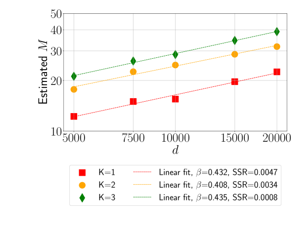
Figure 4: Number of Machines for Support Recovery by DJ-OMP vs. Dimension

Appendix C IMPLEMENTATION DETAILS

The code used to generate the simulations in Section 5 was implemented in Python and was executed on an internal cluster (v3.8; Python Core Team, 2019, PSF licensed). For SIS-based methods, we used the SIS package by Saldana and Feng (2018), which was implemented using R statistical software (v4.0.3; R Core Team, 2023) and embedded into the Python code using the rpy2 package (https://rpy2.github.io/), all licensed by GPL-2 licenses. Lasso-based methods were implemented using the scikit-learn package by Pedregosa et al. (2011, BSD License). Other libraries that were used include NumPy (Harris et al., 2020, liberal BSD license), SciPy (Virtanen et al., 2020, BSD license), and Matplotlib (Hunter, 2007, BSD compatible license).

References

- Acharya et al. (2019) Jayadev Acharya, Chris De Sa, Dylan Foster, and Karthik Sridharan. Distributed learning with sublinear communication. In International Conference on Machine Learning, pages 40–50, 2019.
- Amir et al. (2021) Tal Amir, Ronen Basri, and Boaz Nadler. The trimmed lasso: Sparse recovery guarantees and practical optimization by the generalized soft-min penalty. SIAM journal on mathematics of data science, 3(3):900–929, 2021.
- Amiraz et al. (2021) Chen Amiraz, Robert Krauthgamer, and Boaz Nadler. Tight recovery guarantees for orthogonal matching pursuit under gaussian noise. Information and Inference: A Journal of the IMA, 10(2):573–595, 2021.
- Amiraz et al. (2022) Chen Amiraz, Robert Krauthgamer, and Boaz Nadler. Distributed sparse normal means estimation with sublinear communication. Information and Inference: A Journal of the IMA, 11(3):1109–1142, 2022.
- Barghi et al. (2021) Hanie Barghi, Amir Najafi, and Seyed Abolfazl Motahari. Distributed sparse feature selection in communication-restricted networks. arXiv preprint arXiv:2111.02802, 2021.
- Battey et al. (2018) Heather Battey, Jianqing Fan, Han Liu, Junwei Lu, and Ziwei Zhu. Distributed testing and estimation under sparse high dimensional models. Annals of statistics, 46(3):1352, 2018.
- Ben-Haim et al. (2010) Zvika Ben-Haim, Yonina C Eldar, and Michael Elad. Coherence-based performance guarantees for estimating a sparse vector under random noise. IEEE Transactions on Signal Processing, 58(10):5030–5043, 2010.
- Bertsimas et al. (2016) Dimitris Bertsimas, Angela King, and Rahul Mazumder. Best subset selection via a modern optimization lens. The annals of statistics, 44(2):813–852, 2016.
- Birnbaum (1942) Zygmunt Wilhelm Birnbaum. An inequality for Mill’s ratio. The Annals of Mathematical Statistics, 13(2):245–246, 1942.
- Blumensath and Davies (2008) Thomas Blumensath and Mike E Davies. Iterative thresholding for sparse approximations. Journal of Fourier analysis and Applications, 14(5):629–654, 2008.
- Candes and Tao (2005) Emmanuel J Candes and Terence Tao. Decoding by linear programming. IEEE Transactions on Information Theory, 51(12):4203–4215, 2005.
- Chen et al. (2001) Scott Shaobing Chen, David L Donoho, and Michael A Saunders. Atomic decomposition by basis pursuit. SIAM review, 43(1):129–159, 2001.
- Chen et al. (1989) Sheng Chen, Stephen A Billings, and Wan Luo. Orthogonal least squares methods and their application to non-linear system identification. International Journal of Control, 50(5):1873–1896, 1989.
- Chernoff (1952) Herman Chernoff. A measure of asymptotic efficiency for tests of a hypothesis based on the sum of observations. The Annals of Mathematical Statistics, 23(4):493–507, 1952.
- Chouvardas et al. (2015) Symeon Chouvardas, Gerasimos Mileounis, Nicholas Kalouptsidis, and Sergios Theodoridis. Greedy sparsity-promoting algorithms for distributed learning. IEEE Transactions on Signal Processing, 63(6):1419–1432, 2015.
- Dai and Milenkovic (2009) Wei Dai and Olgica Milenkovic. Subspace pursuit for compressive sensing signal reconstruction. IEEE Transactions on Information Theory, 55(5):2230–2249, 2009.
- Duarte et al. (2005) Marco F Duarte, Shriram Sarvotham, Dror Baron, Michael B Wakin, and Richard G Baraniuk. Distributed compressed sensing of jointly sparse signals. In Asilomar Conference on Signals, Systems and Computers, 2005., pages 1537–1541. IEEE, 2005.
- Fan and Li (2001) Jianqing Fan and Runze Li. Variable selection via nonconcave penalized likelihood and its oracle properties. Journal of the American statistical Association, 96(456):1348–1360, 2001.
- Fan and Lv (2008) Jianqing Fan and Jinchi Lv. Sure independence screening for ultrahigh dimensional feature space. Journal of the Royal Statistical Society Series B: Statistical Methodology, 70(5):849–911, 2008.
- Fonseca and Nadler (2023) Rodney Fonseca and Boaz Nadler. Distributed sparse linear regression under communication constraints. arXiv preprint arXiv:2301.04022, 2023.
- Fosson et al. (2016) Sophie M Fosson, Javier Matamoros, Carles Antón-Haro, and Enrico Magli. Distributed recovery of jointly sparse signals under communication constraints. IEEE Transactions on Signal Processing, 64(13):3470–3482, 2016.
- Gordon (1941) Robert D Gordon. Values of Mills’ ratio of area to bounding ordinate and of the normal probability integral for large values of the argument. The Annals of Mathematical Statistics, 12(3):364–366, 1941.
- Han et al. (2015) Puxiao Han, Ruixin Niu, and Yonina C Eldar. Modified distributed iterative hard thresholding. In 2015 IEEE International Conference on Acoustics, Speech and Signal Processing (ICASSP), pages 3766–3770. IEEE, 2015.
- Harris et al. (2020) Charles R. Harris, K. Jarrod Millman, Stéfan J. van der Walt, Ralf Gommers, Pauli Virtanen, David Cournapeau, Eric Wieser, Julian Taylor, Sebastian Berg, Nathaniel J. Smith, Robert Kern, Matti Picus, Stephan Hoyer, Marten H. van Kerkwijk, Matthew Brett, Allan Haldane, Jaime Fernández del Río, Mark Wiebe, Pearu Peterson, Pierre Gérard-Marchant, Kevin Sheppard, Tyler Reddy, Warren Weckesser, Hameer Abbasi, Christoph Gohlke, and Travis E. Oliphant. Array programming with NumPy. Nature, 585(7825):357–362, September 2020. doi: 10.1038/s41586-020-2649-2. URL https://doi.org/10.1038/s41586-020-2649-2.
- Hastie et al. (2020) Trevor Hastie, Robert Tibshirani, and Ryan Tibshirani. Best subset, forward stepwise or lasso? analysis and recommendations based on extensive comparisons. Statistical Science, 35(4):579–592, 2020.
- Hunter (2007) J. D. Hunter. Matplotlib: A 2d graphics environment. Computing in Science & Engineering, 9(3):90–95, 2007. doi: 10.1109/MCSE.2007.55.
- Jordan et al. (2019) Michael I Jordan, Jason D Lee, and Yun Yang. Communication-efficient distributed statistical inference. Journal of the American Statistical Association, 114(526):668–681, 2019.
- Khanna and Murthy (2016) Saurabh Khanna and Chandra R Murthy. Decentralized joint-sparse signal recovery: A sparse bayesian learning approach. IEEE Transactions on Signal and Information Processing over Networks, 3(1):29–45, 2016.
- Komatu (1955) Yûsaku Komatu. Elementary inequalities for Mills’ ratio. Rep. Statist. Appl. Res. Un. Jap. Sci. Engrs, 4:69–70, 1955.
- Lee et al. (2017) Jason D Lee, Qiang Liu, Yuekai Sun, and Jonathan E Taylor. Communication-efficient sparse regression. The Journal of Machine Learning Research, 18(1):115–144, 2017.
- Li et al. (2015) Gang Li, Thakshila Wimalajeewa, and Pramod K Varshney. Decentralized and collaborative subspace pursuit: A communication-efficient algorithm for joint sparsity pattern recovery with sensor networks. IEEE Transactions on Signal Processing, 64(3):556–566, 2015.
- Ling and Tian (2011) Qing Ling and Zhi Tian. Decentralized support detection of multiple measurement vectors with joint sparsity. In 2011 IEEE International Conference on Acoustics, Speech and Signal Processing (ICASSP), pages 2996–2999. IEEE, 2011.
- Ling et al. (2012) Qing Ling, Zaiwen Wen, and Wotao Yin. Decentralized jointly sparse optimization by reweighted minimization. IEEE Transactions on Signal Processing, 61(5):1165–1170, 2012.
- Liu et al. (2023) Zhan Liu, Xiaoluo Zhao, and Yingli Pan. Communication-efficient distributed estimation for high-dimensional large-scale linear regression. Metrika, 86(4):455–485, 2023.
- Lopes and Yao (2022) Miles E Lopes and Junwen Yao. A sharp lower-tail bound for gaussian maxima with application to bootstrap methods in high dimensions. Electronic Journal of Statistics, 16(1):58–83, 2022.
- Makhzani and Valaee (2013) Alireza Makhzani and Shahrokh Valaee. Distributed spectrum sensing in cognitive radios via graphical models. In 2013 5th IEEE International Workshop on Computational Advances in Multi-Sensor Adaptive Processing (CAMSAP), pages 376–379. IEEE, 2013.
- Mallat and Zhang (1993) Stéphane G Mallat and Zhifeng Zhang. Matching pursuits with time-frequency dictionaries. IEEE Transactions on signal processing, 41(12):3397–3415, 1993.
- Mateos et al. (2010) Gonzalo Mateos, Juan Andrés Bazerque, and Georgios B Giannakis. Distributed sparse linear regression. IEEE Transactions on Signal Processing, 58(10):5262–5276, 2010.
- Miller (2002) Alan Miller. Subset selection in regression. CRC Press, 2002.
- Mota et al. (2011) João FC Mota, João MF Xavier, Pedro MQ Aguiar, and Markus Puschel. Distributed basis pursuit. IEEE Transactions on Signal Processing, 60(4):1942–1956, 2011.
- Needell and Tropp (2009) Deanna Needell and Joel A Tropp. CoSaMP: Iterative signal recovery from incomplete and inaccurate samples. Applied and Computational Harmonic Analysis, 26(3):301–321, 2009.
- Pati et al. (1993) Yagyensh Chandra Pati, Ramin Rezaiifar, and PS Krishnaprasad. Orthogonal matching pursuit: Recursive function approximation with applications to wavelet decomposition. In Conference Record of The Twenty-Seventh Asilomar Conference on Signals, Systems and Computers, pages 40–44. IEEE, 1993.
- Patterson et al. (2014) Stacy Patterson, Yonina C Eldar, and Idit Keidar. Distributed compressed sensing for static and time-varying networks. IEEE Transactions on Signal Processing, 62(19):4931–4946, 2014.
- Pedregosa et al. (2011) F. Pedregosa, G. Varoquaux, A. Gramfort, V. Michel, B. Thirion, O. Grisel, M. Blondel, P. Prettenhofer, R. Weiss, V. Dubourg, J. Vanderplas, A. Passos, D. Cournapeau, M. Brucher, M. Perrot, and E. Duchesnay. Scikit-learn: Machine learning in Python. Journal of Machine Learning Research, 12:2825–2830, 2011.
- Python Core Team (2019) Python Core Team. Python: A dynamic, open source programming language. Python Software Foundation, 2019. URL https://www.python.org/. Python version 3.8.
- R Core Team (2023) R Core Team. R: A Language and Environment for Statistical Computing. R Foundation for Statistical Computing, Vienna, Austria, 2023. URL https://www.R-project.org/.
- Rosenblatt and Nadler (2016) Jonathan D Rosenblatt and Boaz Nadler. On the optimality of averaging in distributed statistical learning. Information and Inference: A Journal of the IMA, 5(4):379–404, 2016.
- Saldana and Feng (2018) Diego F Saldana and Yang Feng. SIS: An R package for sure independence screening in ultrahigh-dimensional statistical models. Journal of Statistical Software, 83(2):1–25, 2018. doi: 10.18637/jss.v083.i02.
- Shamir (2014) Ohad Shamir. Fundamental limits of online and distributed algorithms for statistical learning and estimation. In Advances in Neural Information Processing Systems, pages 163–171, 2014.
- Šidák (1967) Zbyněk Šidák. Rectangular confidence regions for the means of multivariate normal distributions. Journal of the American Statistical Association, 62(318):626–633, 1967.
- Steinhardt and Duchi (2015) Jacob Steinhardt and John Duchi. Minimax rates for memory-bounded sparse linear regression. In Conference on Learning Theory, pages 1564–1587, 2015.
- Sundman et al. (2012) Dennis Sundman, Saikat Chatterjee, and Mikael Skoglund. A greedy pursuit algorithm for distributed compressed sensing. In 2012 IEEE International Conference on Acoustics, Speech and Signal Processing (ICASSP), pages 2729–2732. IEEE, 2012.
- Sundman et al. (2014) Dennis Sundman, Saikat Chatterjee, and Mikael Skoglund. Distributed greedy pursuit algorithms. Signal Processing, 105:298–315, 2014.
- Tibshirani (1996) Robert Tibshirani. Regression shrinkage and selection via the lasso. Journal of the Royal Statistical Society. Series B (Methodological), 58:267–288, 1996.
- Tropp (2004) Joel A Tropp. Greed is good: Algorithmic results for sparse approximation. IEEE Transactions on Information Theory, 50(10):2231–2242, 2004.
- Tropp and Gilbert (2007) Joel A Tropp and Anna C Gilbert. Signal recovery from random measurements via orthogonal matching pursuit. IEEE Transactions on Information Theory, 53(12):4655–4666, 2007.
- Virtanen et al. (2020) Pauli Virtanen, Ralf Gommers, Travis E. Oliphant, Matt Haberland, Tyler Reddy, David Cournapeau, Evgeni Burovski, Pearu Peterson, Warren Weckesser, Jonathan Bright, Stéfan J. van der Walt, Matthew Brett, Joshua Wilson, K. Jarrod Millman, Nikolay Mayorov, Andrew R. J. Nelson, Eric Jones, Robert Kern, Eric Larson, C J Carey, İlhan Polat, Yu Feng, Eric W. Moore, Jake VanderPlas, Denis Laxalde, Josef Perktold, Robert Cimrman, Ian Henriksen, E. A. Quintero, Charles R. Harris, Anne M. Archibald, Antônio H. Ribeiro, Fabian Pedregosa, Paul van Mulbregt, and SciPy 1.0 Contributors. SciPy 1.0: Fundamental Algorithms for Scientific Computing in Python. Nature Methods, 17:261–272, 2020. doi: 10.1038/s41592-019-0686-2.
- Wang et al. (2017) Jialei Wang, Mladen Kolar, Nathan Srebro, and Tong Zhang. Efficient distributed learning with sparsity. In International Conference on Machine Learning, pages 3636–3645, 2017.
- Wimalajeewa and Varshney (2013) Thakshila Wimalajeewa and Pramod K Varshney. Cooperative sparsity pattern recovery in distributed networks via distributed-OMP. In 2013 IEEE International Conference on Acoustics, Speech and Signal Processing, pages 5288–5292. IEEE, 2013.
- Wimalajeewa and Varshney (2014) Thakshila Wimalajeewa and Pramod K Varshney. OMP based joint sparsity pattern recovery under communication constraints. IEEE Transactions on Signal Processing, 62(19):5059–5072, 2014.
- Wimalajeewa and Varshney (2017) Thakshila Wimalajeewa and Pramod K Varshney. Application of compressive sensing techniques in distributed sensor networks: A survey. arXiv preprint arXiv:1709.10401, 2017.