MIXRTs: Toward Interpretable Multi-Agent Reinforcement Learning via Mixing Recurrent Soft Decision Trees

Abstract

While achieving tremendous success in various fields, existing multi-agent reinforcement learning (MARL) with a black-box neural network architecture makes decisions in an opaque manner that hinders humans from understanding the learned knowledge and how input observations influence decisions. Instead, existing interpretable approaches, such as traditional linear models and decision trees, usually suffer from weak expressivity and low accuracy. To address this apparent dichotomy between performance and interpretability, our solution, MIXing Recurrent soft decision Trees (MIXRTs), is a novel interpretable architecture that can represent explicit decision processes via the root-to-leaf path and reflect each agent’s contribution to the team. Specifically, we construct a novel soft decision tree to address partial observability by leveraging the advances in recurrent neural networks, and demonstrate which features influence the decision-making process through the tree-based model. Then, based on the value decomposition framework, we linearly assign credit to each agent by explicitly mixing individual action values to estimate the joint action value using only local observations, providing new insights into how agents cooperate to accomplish the task. Theoretical analysis shows that MIXRTs guarantees the structural constraint on additivity and monotonicity in the factorization of joint action values. Evaluations on the challenging Spread and StarCraft II tasks show that MIXRTs achieves competitive performance compared to widely investigated methods and delivers more straightforward explanations of the decision processes. We explore a promising path toward developing learning algorithms with both high performance and interpretability, potentially shedding light on new interpretable paradigms for MARL.

1 Introduction

Multi-agent reinforcement learning (MARL) has proven to be a considerable promise for addressing a variety of challenging tasks, e.g., games [1, 2, 3], autonomous driving [4, 5] and robotics interactions [6, 7]. Despite its promising performance, the advancements are mainly attributed to utilizing deep neural network (DNN) models as powerful function approximators, which are encoded with thousands to millions of parameters interacting in complex and nonlinear ways [8]. This complexity of architecture brings substantial obstacles for humans to understand how decisions are made and what key features influence decisions, especially when the network grows deeper in size or more complex structures are appended [9, 10]. Indeed, creating mechanisms to interpret the implicit behaviors of black-box DNNs remains an open problem in the field of machine learning [11, 12].

It is crucial to gain insights into the decision-making process of artificially intelligent agents for successful and reliable deployments into real-world applications, especially in high-stakes domains such as healthcare, aviation, and public policy making [13, 14, 15, 16]. Significant limitations are imposed on practitioners applying MARL techniques, as the lack of transparency creates critical barriers to establishing trust in the learned policies and scrutinizing policy weaknesses [17]. Explainable reinforcement learning [18, 19, 20] stands as a promising avenue for the formulation of transparent procedures that can be followed step-by-step or held accountable by human operators. While existing explainable methods offer some potential [21, 22] or provide vision-based interpretations [23] in single-agent tasks, they are still struggling to strike a balance between trustworthy model interpretability and matching the performance in look-ahead reinforcement learning [24], especially in multi-agent domains.

Traditional decision trees [25, 26] present lightweight inferences to interpretability, as humans can easily understand the decision process by visualizing decision pathways. However, traditional decision trees may suffer from weak expressivity and therefore low accuracy with a shallow tree depth and univariate decision nodes, making it a hard trade-off between model interpretability and learning performance. Alternatively, differentiable soft decision trees (SDTs) [27, 28], based on the structure of fuzzy decision trees, model expressivity lies in the middle of traditional decision trees and neural networks [29]. SDTs are acclaimed for their comprehensibility, offering interpretations that non-expert individuals can easily visualize and simulate, thereby enhancing human readability. Several works [30, 31] attempt to utilize an imitation learning paradigm to distill a pre-trained DNN control policy into an SDT, providing an interpretable form of policy in single-agent tasks. However, the inherent opacity of DNN structures imposes constraints on the SDT’s capacity to accurately mimic the DNN policy. It thus poses a challenge to jointly maintaining the mimic fidelity and the simplicity of tree models to find a “sweet spot”.

Rather than imitating a pre-trained policy, an alternative is to train an SDT policy from agent experience in an end-to-end manner, which directly learns the domain knowledge from the tasks using interpretable models. While SDT has achieved an adequate balance between interpretability and performance in simple single-agent domains (e.g., CartPole and MountainCar in OpenAI Gym [32]) [31], they cannot maintain satisfying learning performance without sacrificing interpretability in complex multi-agent tasks due to limited model expressivity. Particularly, to the best of our knowledge, there is seldom existing work exploring the model interpretability in MARL domains. Here, we aim at a more efficient and explicit interpretable architecture with tree-based models in multi-agent challenging tasks.

In this paper, we propose a novel MIXing Recurrent soft decision Trees (MIXRTs) method to tackle the tension between model interpretability and learning performance in MARL domains. Instead of trying to understand how a DNN makes its decisions, we utilize the differentiable SDT to keep the decision-making process. First, to facilitate learning over long timescales for each agent, we propose the recurrent tree cell (RTC) that receives the current individual observation and history information as input at each timestamp. Second, we utilize a linear combination of multiple RTCs with an ensemble mechanism to improve performance and reduce the variance of SDTs, while maintaining the interpretability of RTCs. By visualizing the tree structure, RTCs can provide intuitive explanations of how important features affect the decision process. MIXRTs consists of individual RTCs representing the individual value function, and a mixing tree structure aiming to learn an optimal linear value decomposition, which ensures consistency between the centralized and decentralized policies. The linear mixing structure emphasizes the explanations about what role each agent plays in cooperative tasks by analyzing its assigned credit. To improve learning efficiency, we utilize parameters sharing across individual RTCs to dramatically reduce the number of policy parameters, while experience can be shared across other agents. We evaluate MIXRTs on a range of challenging tasks in Spread and StarCraft II [33] environment. Empirical results substantiate that our learning architecture delivers simple explanations while enjoying competitive performance. Specifically, MIXRTs finds desirable optimal policies in easy scenarios compared to the baselines like the widely investigated QMIX [3] and QPLEX [34].

The remaining paper is organized as follows. In Section 2, we introduce basic concepts of MARL, SDTs, and related work. In Section 3 and 4, we present the RTCs and the linear mixing architecture of individual RTCs, respectively. In Section 5, we give experimental results of learning performance compared to the existent baselines. The comprehensive interpretability of our model and the results of the user study are given in Section 6. Finally, we give concluding remarks in Section 7.

2 Background and related works

2.1 Preliminaries

Dec-POMDP. The fully cooperative multi-agent task is generally modeled as a decentralized partially observable Markov decision process (Dec-POMDP) [35] that consists of a tuple $\left<\mathcal{S},\mathcal{U},\mathcal{P},r,\mathcal{Z},\mathcal{O},n,\gamma\right>$, where $s\in\mathcal{S}$ describes the global state of the environment. At each time step, each agent $i\in\{1,...,n\}$ only receives a partial observation $o_{i}\in\mathcal{Z}$ from an observation function $\mathcal{O}(s,i)$, and chooses an action $u_{i}\in\mathcal{U}$ to formulate a joint action $\bm{u}:=\left[u_{i}\right]_{i=1}^{n}\in\mathcal{U}^{n}$. This results in a transition to next state $s^{\prime}\sim P\left(s^{\prime}\mid s,\bm{u}\right)$. All agents share the same team reward signal $r(s,\bm{u}):\mathcal{S}\times\mathcal{U}^{n}\rightarrow\mathbb{R}$. Furthermore, each agent learns its own policy $\pi_{i}\left(u_{i}\mid\tau_{i}\right):\mathcal{T}\times\mathcal{U}\rightarrow[0,1]$, which conditions on the its action-observation history denoted as $\tau_{i}\in\mathcal{T}:=(\mathcal{Z}\times\mathcal{U})^{*}$. The goal is to find an optimal joint policy $\bm{\pi}=\left\langle\pi_{1},\ldots,\pi_{n}\right\rangle$ to maximize the discounted cumulative return $\sum_{t=0}^{\infty}\gamma^{t}r^{t}$, where the discount factor is $\gamma\in[0,1)$.

Multi-agent Q-learning in Dec-POMDP. Q-learning [36] is a classic tabular model-free algorithm to find the optimal joint action-value function $Q^{*}(s,\bm{u})=r(s,\bm{u})+\gamma\mathbb{E}_{s^{\prime}}[\max_{\bm{u}^{\prime}\in\mathcal{U}^{n}}$ $Q^{*}\left(s^{\prime},\bm{u}^{\prime}\right)]$. Multi-agent Q-learning approaches [2, 37, 38] are based on the value decomposition extension of deep Q-learning [36, 39], thus the agent system receives the joint action-observation history $\bm{\tau}$ and the joint action $\bm{u}$. Given transition tuples $(\bm{\tau},\bm{u},r,\bm{\tau^{\prime}})$ from the replay buffer $\mathcal{B}$, the network parameters $\mathit{\Theta}$ are learnt by minimizing the squared loss $\mathcal{L}(\mathit{\Theta})$ on the temporal-difference (TD) error $\sigma=y^{\prime}-Q_{tot}(\bm{\tau},\bm{u};\mathit{\Theta})$, where $y^{\prime}=r+\gamma\,\max_{\bm{u^{\prime}}}Q_{tot}(\bm{\tau^{\prime}},\bm{u^{\prime}};\mathit{\Theta^{\prime}})$ is the target and $Q_{tot}(\bm{\tau},\bm{u};\mathit{\Theta})$ is used in place of $Q_{tot}(s,\bm{u};\mathit{\Theta})$ due to partial observability. The parameters $\mathit{\Theta^{\prime}}$ from a target network are periodically copied from $\mathit{\Theta}$ and remain constant over multiple iterations.

Centralized training and decentralized execution (CTDE). In the CTDE fashion, action-observation values of all agents and global states are collected through a central controller during training. However, in the execution phase, each agent has its own policy network to make decisions based on its individual action-observation history. The individual-global-max (IGM) property [37] is a popular principle to realize effective CTDE as

$$\arg\underset{\bm{u}\in\mathcal{U}^{n}}{\max}\,Q_{tot}(\bm{\tau},\bm{u})=\begin{pmatrix}\arg\underset{u_{1}\in\mathcal{U}}{\max}\,Q_{1}(\tau_{1},u_{1})\\ \vdots\\ \arg\underset{u_{n}\in\mathcal{U}}{\max}\,Q_{n}(\tau_{n},u_{n})\end{pmatrix},$$ (1)

where $\bm{\tau}$ represents the history record of joint action-observation and $Q_{tot}$ represents the joint Q-function for each individual action-value function $Q_{i}(\tau_{i},u_{i})$. Both VDN [2] and QMIX [3] are popular CTDE methods for estimating the optimal $Q_{tot}$ via the combined agents of $Q_{i}$. In VDN, the $Q_{tot}$ is calculated by summing the utilities of each agent as $Q_{tot}(\bm{\tau},\bm{u})=\sum_{i=1}^{n}Q_{i}(\tau_{i},u_{i})$. QMIX combines $Q_{i}$ through the state-dependent nonlinear monotonic function $f_{s}$: $Q_{tot}(\bm{\tau},\bm{u})=f_{s}(Q_{1}(\tau_{1},u_{1}),...,Q_{i}(\tau_{i},u_{i}),...,Q_{n}(\tau_{n},u_{n}))$, where $\frac{\partial f_{s}}{\partial Q_{i}}\geq 0,\forall i\in\{1,...,n\}$.

Soft decision trees (SDTs). Differentiable decision trees [40, 41] have been shown to be more accurate compared to traditional hard decision trees. Especially, an SDT [27] with binary probabilistic decision boundary at each node has favorable transparency and performance in reinforcement learning tasks [30, 31]. As shown in Fig. 1(a), SDT fixes the depth of the tree in advance and performs path selection by probability, which is different from the traditional growth way of learning crisp decision boundaries. By giving an observation $o^{t}$, each inner node $j$ calculates the probability for traversing to the left child node as

$$p_{j}(o^{t})=\sigma(w_{o}^{j}o^{t}+b^{j}),$$ (2)

where $\sigma$ is the sigmoid function, $w^{j}$ and $b^{j}$ are trainable parameters. The learned model consists of a hierarchy of decision filters that assign the input observation to a particular leaf node with a particular path probability $P^{l}(o^{t})$, producing a probability distribution over the $\mathcal{U}$ action class. Each leaf $l\in\mathit{LeafNodes}$ encodes relative activation values $Q^{l}=\text{softmax}(\theta^{l})$, where $\theta^{l}\in\mathbb{R}^{\mathcal{U}}$ is a learnable parameter at the $l$-th leaf. Following SDT, we select an action with the largest probability leaf $Q^{l_{\max}}$ as the overall classification decision, where $l_{\max}=\arg\max_{l}P^{l}(o^{t})$.

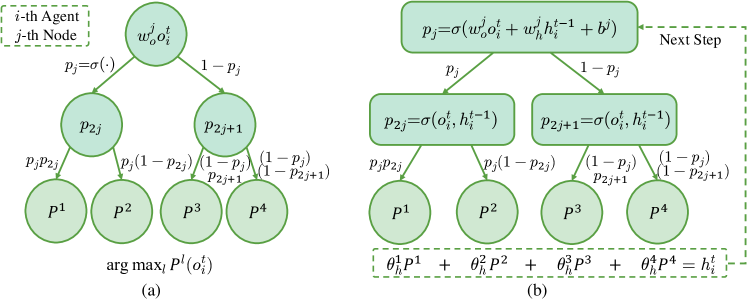
Figure 1: Examples of SDT and RTC. (a) A two-level SDT. (b) Illustration of the process of a two-level RTC that receives the current individual observation $o^{t}_{i}$ and the historical leaf information $h^{t-1}_{i}$ as input at each timestamp.

2.2 Related works

Explainable reinforcement learning. In the reinforcement learning community, a number of prior works have started exploring approaches that lead to interpretable policies via intrinsic methods [28, 40, 41, 42]. Intrinsic methods generally rely on using inherently interpretable models such as classical decision trees and linear models, which directly represent the faithful decision-making process. Conservative Q-improvement method [42] presents an interpretable decision-tree model that learns a policy in the form of a hard decision tree for the robot navigation tasks. It can better trade off the performance and simplicity of the policy model by adding a new split only if doing so could improve the policy. Differentiable decision trees methods [28, 43] allow for a gradient update over Q-learning and policy gradient algorithms by replacing the Boolean decision with the sigmoid activation function at the decision node, which improves the performance while affording interpretable tree-based policies. Rather than incrementally adding nodes, differentiable decision trees produce the trees entirely over the learning process, where the leaf nodes represent single features with the discretization technique for improving interpretability. Instead of constructing a univariate decision tree, cascading decision tree (CDT) [31], as an extension based on SDT with multivariate decision nodes, applies representation learning to the decision path to allow richer expressivity. The prior works closest to ours are SDT [27] and CDT [31], which policies are generated by the routing probabilities at each leaf node to make decisions. Our method differs in that 1) we introduce the recurrency into SDTs for capturing the long-term condition in partially observable tasks, 2) we explicitly present the graphical decision process with less depth by considering all variate at each node instead of univariate feature, and 3) we interpret the role each agent plays in the team by visualizing the linear credit assignment.

Cooperative multi-agent reinforcement learning. Dating back to the early stage of MARL, independent Q-learning [44] is the most commonly used method where each agent myopically optimizes its individual policy that is independent of the others. Generally, they only observe local information, execute their own actions, and receive their rewards individually such that other agents are perceived as part of the environment. This approach has no theoretical convergence guarantee like Q-learning for ignoring the nonstationarity induced by the changes of the other agents. By contrast, CTDE [45, 46] is an advanced paradigm for cooperative MARL tasks, which allows each agent to learn their individual utility functions via optimizing the joint action-value function for credit assignment. VDN [2] factorizes the joint action-value function into a linear summation over individual agents. To overcome the VDN’s limitations that ignore extra global state information, QMIX [3] utilizes a network to estimate joint action-value function with a non-linear combination of each agent value. QTRAN [37] relaxes these constraints of the greedy action selections between the joint and individual value functions with two soft regularizations. Different from QTRAN which loses the exact IGM consistency, QPLEX [34] uses a dueling network architecture to represent both joint and individual action-value functions to guarantee the IGM property.

Our proposed MIXRTs is distinguished from the above representative value decomposition methods in the following ways: 1) our method builds upon soft decision trees; our RTCs not only produces an intrinsically interpretable model for visualizing the decision-making process instead of the complex neural network architecture but also achieve competitive performance. 2) Our mixing trees module linearly factorizes the joint action-value function into individual action-value, achieving high scalability with a full realization of the IGM principle. Benefiting from the interpretable model, we can explain not only the explicit behavior of the individual agent but also the behavior of different roles in the allies. 3) Our artful designs yield lightweight inference, whilst achieving competitive performance on a range of cooperative challenging tasks.

3 Recurrent Tree Cells

In this section, we propose RTCs that introduces recurrency into SDTs to encode the previous information and enhance the fidelity of the Q-value with the ensemble technique. First, we propose an RTC that receives the current individual observation and relies on historical information to capture long-term dependencies in partially observable tasks. Then, we utilize a linear combination of multiple RTCs via an ensemble mechanism to yield high performance and reduce the variance of the model while retaining simplicity and interpretability.

3.1 Recurrent Tree Cell

The complexity of neural networks brings barriers to understanding, verifying, and trusting the behavior of the agent, as it has complex transformations and nests non-linear operators. To relieve the dilemma, SDT offers an effective way to interpret the decision-making pathways by visualizing decision nodes and associated probabilities. As depicted in Fig. 1(a), SDT is an univariate differentiable tree with a probabilistic decision boundary at each filter. However, SDT has no explicit mechanisms for deciphering the underlying state of POMDP in sequential decision-making tasks over longer timescales. Generally, it could degrade the performance by estimating the Q-value from an incomplete observation instead of a global state. Indeed, by leveraging recurrency to a deep Q-network with a recurrent neural network (RNN), agents can effectively capture long-term dependencies conditioning on their entire action-observation history [47]. Inspired by the advances in the recurrent architecture, we first introduce recurrency into the SDT structure and propose a recurrent tree cell (RTC) to encode long-term dependencies. As shown in Fig. 1(b), RTC receives the current individual observation $o^{t}_{i}$ and history embedding $h^{t-1}_{i}$ as input at each time step, and extracts the information of the previous hidden state for each agent $i$.

Combining the recurrent architecture, for each non-leaf node, RTC learns linear filters in its branching node to traverse to the left child node with the probability as

$$p_{j}(o_{i}^{t},h_{i}^{t-1})=\sigma(w^{j}_{o}o_{i}^{t}+w^{j}_{h}h_{i}^{t-1}+b^{j}),$$ (3)

where $b^{j}$ is a learnable bias parameter, and $w^{j}_{o}$ and $w^{j}_{h}$ are the learnable parameters for the feature vectors of the observation $o^{t}_{i}$ and the previous hidden state $h^{t-1}_{i}$, respectively. Similarly, we can obtain the probability of the right branch as $1-p_{j}(o_{i}^{t},h_{i}^{t-1})$, which is the same as in SDT. Then, for each leaf node, the probability of selecting the leaf $P^{l}$ is equal to the product of the overall path probability starting from the root to the leaf node $l$ as

$$P^{l}(o_{i}^{t},h_{i}^{t-1})=\prod_{j\in route(l)}\left\{p_{\left\lfloor j/2\right\rfloor\rightarrow j}(o_{i}^{t},h_{i}^{t-1})^{\left[l\swarrow j\right]}\,\right.$$ (4)

$$\left.(1-p_{\left\lfloor j/2\right\rfloor\rightarrow j}(o_{i}^{t},h_{i}^{t-1}))^{1-\left[l\swarrow j\right]}\right\},$$

where $\left[l\swarrow j\right]$ denotes the boolean event $\in\left\{0,1\right\}$, which means whether $j$ passes the left-subtree to reach the leaf node $l$. With the target distribution of the tree, we measure the current hidden state $h_{i}^{t}$ of the leaf by combining the probability values of each leaf with the weight scalar $\theta^{l}_{h}$ and provide a vector $w_{q}$ that serves this tree to capture the action-observation value as

$$h_{i}^{t}= \sum_{l\in\mathit{LeafNodes}}P^{l}(o_{i}^{t},h_{i}^{t-1})\,\theta^{l}_{h},$$ (5)

$$Q_{i}(\tau_{i},\cdot)= ~{}~{}~{}~{}~{}~{}h_{i}^{t}\,w_{q},$$

where $P^{l}$ is the overall path probability along the root to the leaf $l$. Different from the leaf nodes of SDT, the learnable parameter $\theta^{l}_{h}\in\mathbb{R}$ in an RTC calculates the hidden state $h_{i}^{t}$ by multiplying with $P^{l}$, and $w_{q}\in\mathbb{R}^{\mathcal{U}}$ is a training parameter to transform the hidden information $h_{i}^{t}$ into the action distribution. Finally, in a decentralized execution way, we choose an action $u_{i}^{t}$ for each agent $i$ by $\varepsilon$-greedy methods with respect to its $Q_{i}(\tau_{i},u_{i})$. This decision process retains the simplicity and interpretability of the model since it can present which dimensions of observation influence the action distribution during the inference.

3.2 Ensemble of Recurrent Tree Cells

The SDT-based methods exhibit several appealing properties with the multivariate tree structure, such as ease of tuning, robustness to outliers and good interpretability [31]. Since all input features are used for each node with a multivariate setting, a single SDT could lack expressiveness and output predictions with high variance. An ensemble paradigm of models, rather than a single one, is well known to reduce the variance component of the estimation error [48, 49]. To relieve the above tension while maintaining the interpretability, we linearly combine multiple RTCs with the variance-optimized bagging (Vogging) approach based on the bagging technique [50]. Based on the Vogging ensemble mechanism, the individual value function for the agent $i$ can be represented as

$$Q_{i}(\tau_{i},\cdot)=h_{i,(1)}^{t}\,w_{q,(1)}+h_{i,(2)}^{t}\,w_{q,(2)}+...+h_{i,(H)}^{t}\,w_{q,(H)},$$ (6)

where $H$ is the size of ensemble RTCs, $w_{q,(1)},w_{q,(2)},...,w_{q,(H)}$ are learnable parameters to optimize a linear combination of the $H$ trees for improving the expressiveness and reducing the prediction variance of RTCs, and the hidden state $h^{t}_{i}\in\mathbb{R}^{H}$ is derived as the vector $[h_{i,(1)}^{t},h_{i,(2)}^{t},...,h_{i,(H)}^{t}]$ to express the history record. Finally, the RTCs produces a local policy distribution as a Q-function for each agent and execute the action via sampling the distribution. Here, we utilize back-propagating gradients to update the $Q_{i}$ from the Q-learning rule [36, 39] via the joint reward over all agents.

Remark 1.

The functions used for all sub-modules in the RTCs ensemble are linear, which both maintains the interpretability of the model and simplifies it. Note that when the model structure gets complex, the interpretability decreases as the simplicity of the model is lost. Since shallow trees can be easily described and even be implemented by hand, it is acceptable that linearly combining the trees of depth $2$ or $3$ achieves acceptable performance and stability via only sacrificing a little bit model interpretability. In practice, a moderate number of ensemble trees $H$ (e.g., $16\sim 64$) is sufficient to obtain efficient performance, and additional ablation results are provided in Section 8.

4 Mixing Recurrent SDTs Architecture

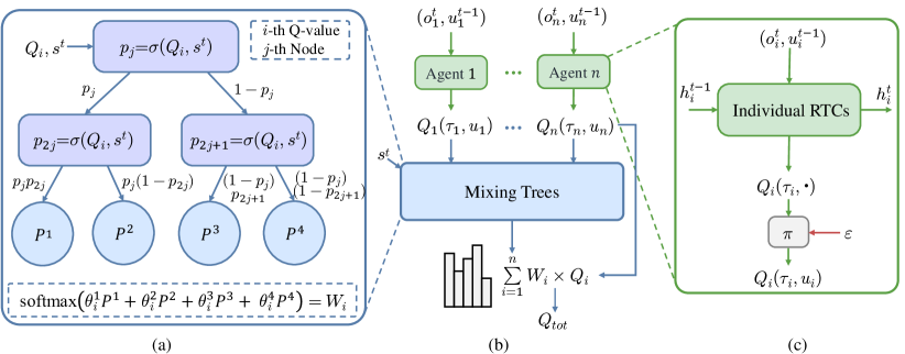
Figure 2: MIXRTs architecture. (a) Diagram of the structure of the mixing tree with depth $2$. (b) In the overall MIXRTs architecture, we finally obtain the joint $Q_{tot}$ value via a linear combination of the individual action-value functions. (c) An individual RTCs structure for each agent.

In this section, we propose a novel method called MIXing Recurrent soft decision Trees (MIXRTs), which can represent a much richer class of action-value functions analogous to the advanced CTDE algorithms. The overall architecture of MIXRTs is illustrated in Fig. 2, including two main components as follows: (i) an ensemble of RTCs as an individual action-value function for each agent, and (ii) a mixing component similar to the ensemble of RTCs in which a joint action-value function $Q_{tot}$ is factorized into the individual action-value function $Q_{i}$ of each agent $i$ under the IGM constraint. The two components are trained in a centralized manner and each agent uses its own factorized individual action-value function $Q_{i}$ to take actions during decentralized execution. Each component is elaborated on next.

4.1 Individual RTCs for the Action Value

For each agent, the individual action-value function generally could be represented by an ensemble of RTCs, where different agents are mutually independent RTCs. However, the joint action-observation space grows exponentially as the number of agents increases, and then its large number of learnable parameters may cause confusion in understanding the decision process of the model. Inspired by parameters sharing [2], we utilize the ensemble of RTCs to share certain parameters of RTCs between agents for improving the learning efficiency, which can also give rise to the concept of agent invariance and help avoid the lazy agent problem. To keep the agent invariance, we incorporate the role information into the agent via a one-hot encoding of its identity, and the role information is concatenated with the corresponding observation at the root layer. The architecture, with shared weights and information channels across agent networks, satisfies agent invariance with the identical policy and improves simplicity and interpretability with fewer parameters. For each agent $i$, the individual value is represented by an ensemble of RTCs, which takes the current local observation $o^{t}_{i}$, the previous hidden state $h^{t-1}_{i}$ and the previous action $u^{t-1}_{i}$ as the inputs, and then outputs the local action-value $Q_{i}(\tau_{i},u_{i})$.

4.2 Mixing Trees Architecture

The mixing trees architecture follows an interpretable Q-value decomposition formation that connects the local and joint action-value functions via feed-forward ensemble trees, which is also similar to the ensemble of RTCs without embedding the history information. It incorporates the information of global state $s_{t}$ into individual action-value functions during the centralized training process and produces the weights of the local action-value in the joint action-value $Q_{tot}$. The main assumption is that the joint action-value function can be additively decomposed into value functions across agents. However, unlike VDN or QMIX, we assume that the joint action-value function can be approximately weighted by the individual Q-values in a linear manner as

$$Q_{tot}(\bm{\tau},\bm{u})\approx\sum_{i=1}^{n}W_{i}Q_{i}(\tau_{i},u_{i}),$$ (7)

where $\mathbf{\bm{\tau}}$ and $\bm{u}$ are joint action-observation and joint action, respectively, and we force the assignment of credit weights $W_{i}>0$. The choice of linear weighting aims to render a reliable interpretation of the relationship between the agents. Generally, the agent who receives a higher credit assignment with a larger weight $W_{i}$ makes a greater contribution to the team.

In detail, we employ the interpretable RTCs to obtain the weights $W_{i}$ for each agent $i$, which establishes the relations from the individuals to the global. Each root of the ensemble of RTCs takes the individual action-value $Q_{i}$ and the global state vector $s^{t}$ as input as

$$p_{j}(Q_{i},s^{t})=\sigma(w^{j}_{q}Q_{i}+w^{j}_{s}s^{t}+b^{j}),$$ (8)

where $w^{j}_{q}$, $w^{j}_{s}$, and $b^{j}$ are learnable parameters for each layer of the RTC. After the inference process, we can obtain the joint probability distributions $P^{l}$ at the leaf node layer. Here, we utilize the same operation as the individual action-value RTCs with $H$ trees to obtain the stable weights as

$$\phi_{i}= \sum_{l\in\mathit{LeafNodes}}P^{l}(Q_{i},s^{t})\,\theta^{l}_{i},$$ (9)

$$W_{i}= \frac{exp(\sum_{k=1}^{H}\phi_{i,(k)}\,w_{\phi,(k)})}{\sum_{i=1}^{n}exp(\sum_{k=1}^{H}\phi_{i,(k)}\,w_{\phi,(k)})},$$

where $\theta^{l}_{i},w_{\phi}$ are the learnable parameters and the mixing weight $W_{i}$ is positive with softmax operation to enforce the monotonicity between $Q_{tot}$ and each $Q_{i}$. Here, the ultimate goal of the mixing architecture is not only to describe the realization of efficient value decomposition, but also to elaborate an intuitive interpretation that produces the importance of observation attributes and the weight of each agent at different time steps for one episode. Further, Theorem 1 presents the theoretical analysis that MIXRTs guarantees the monotonicity by imposing an easy constraint on the relationship between $Q_{tot}$ and each $Q_{i}$, which is sufficient to satisfy Eq. 1. This allows each agent $i$ to participate in a decentralized execution solely by choosing greedy actions.

Theorem 1.

Let $Q_{tot}(\bm{\tau},\bm{u})$ be a joint action-value function that is factorized by a set of individual action-value functions $Q_{i}(\tau_{i},u_{i})$ as $Q_{tot}(\bm{\tau},\bm{u})\approx\sum_{i=1}^{n}W_{i}Q_{i}(\tau_{i},u_{i})$, where $W_{i}>0$ and $n$ is the number of agents. Then, we have $\bm{u^{\ast}}=\arg\max_{\bm{u}\in\mathcal{U}^{n}}Q_{tot}(\bm{\tau},\bm{u})$ that satisfies the IGM principle.

Proof.

For an arbitrary factorizable $Q_{tot}(\bm{\tau},\bm{u})$, we take $\bm{u^{\ast}}=\arg\max_{\bm{u}\in\mathcal{U}^{n}}Q_{tot}(\bm{\tau},\bm{u})$. Recall that $\bm{u^{\ast}}:=\left[u^{\ast}_{i}\right]_{i=1}^{n}\in\mathcal{U}^{n}$ and $u^{\ast}_{i}=\arg\max_{u_{i}\in\mathcal{U}}Q_{i}(\tau_{i},u_{i})$. After the softmax operation, the weight of each individual action-value function satisfies $W_{i}>0$. For $\forall i\in\{1,2,...,n\}$, we have monotonicity, i.e.,

$$\frac{\partial Q_{tot}}{\partial Q_{i}}>0.$$ (10)

Thus, for any $\left[u_{i}\right]_{i=1}^{n}$ and the mixing trees function $Q_{tot}(\cdot)$ with $n$ weights, the following holds

$$\ \ \ \ \ \ Q_{tot}(Q_{1}(\tau_{1},u_{1}),Q_{2}(\tau_{2},u_{2}),\cdots,Q_{n}(\tau_{n},u_{n}))$$

$$:=W_{1}Q_{1}(\tau_{1},u_{1})+W_{2}Q_{2}(\tau_{2},u_{2})+\cdots+W_{n}Q_{n}(\tau_{n},u_{n})$$

$$\leq W_{1}Q_{1}(\tau_{1},u^{\ast}_{1})+W_{2}Q_{2}(\tau_{2},u^{\ast}_{2})+\cdots+W_{n}Q_{n}(\tau_{n},u^{\ast}_{n}).$$

Thus, according to the $\arg\max$ operator, we have the maximum of the joint action value

$$\,\,\,\,\ \ \,\ \underset{\bm{u}\in\mathcal{U}^{n}}{\max}\,Q_{tot}(\bm{\tau},\bm{u})$$

$$:=\underset{\bm{u}\in\mathcal{U}^{n}}{\max}\,Q_{tot}(Q_{1}(\tau_{1},u_{1}),Q_{2}(\tau_{2},u_{2}),\cdots,Q_{n}(\tau_{n},u_{n}))$$

$$\ =Q_{tot}(Q_{1}(\tau_{1},u^{\ast}_{1}),Q_{2}(\tau_{2},u^{\ast}_{2}),\cdots,Q_{n}(\tau_{n},u^{\ast}_{n})).$$

Hence, we have $\bm{u^{\ast}}=\arg\max_{\bm{u}\in\mathcal{U}^{n}}Q_{tot}(\bm{\tau},\bm{u})$ that satisfies the IGM principle, and the assumed mixing trees provide universal function approximation weights by Eq. (7). ∎

All parameters $\mathit{\Theta}$ in MIXRTs are learned by sampling a number of transitions $b$ from the buffer $\mathcal{B}$ and minimizing the following expected squared temporal difference (TD) error loss as

$$\mathcal{L}(\mathit{\Theta})=\mathbb{E}_{(\mathbf{\bm{\tau}},\bm{u},r,\mathbf{\bm{\tau}}^{\prime})\in b}\left[(y^{\prime}-Q_{tot}(\mathbf{\bm{\tau}},\bm{u};\mathit{\Theta}))^{2}\right],$$ (11)

and the target is obtained via Double DQN [51, 52], which estimates as $y^{\prime}=r+\gamma\overline{Q}_{tot}(\bm{\tau^{\prime}},\arg\max_{\bm{u^{\prime}}\in\mathcal{U}^{n}}{Q}_{tot}(\mathbf{\bm{\tau^{\prime}}},\bm{u^{\prime}};\mathit{\Theta^{\prime}}))$. $\mathit{\Theta^{\prime}}$ are the parameters of a target network that are periodically copied from $\mathit{\Theta}$. Since Eq. (1) holds, we maximize $Q_{tot}$ in a linear fashion to achieve competitive performance, rather than scaling the non-linear case.

TABLE I: The StarCraft multi-agent challenge benchmark.

Scenarios Type	Map	Ally Units	Enemy Units	Total Steps
Easy	3m	3 Marines	3 Marines	$1050K$
	8m	8 Marines	8 Marines	$1500K$
	2s3z	2 Stalkers, 3 Zealots	2 Stalkers, 3 Zealots	$1500M$
	2s_vs_1sc	2 Stalkers	1 Spine Crawler	$2M$
Hard	5m_vs_6m	5 Marines	6 Marines	$2M$
	3s5z	3 Stalkers, 5 Zealots	3 Stalkers, 5 Zealots	$2M$
	8m_vs_9m	8 Marines	9 Marines	$2M$
Super Hard	6h_vs_8z	6 Hydralisks	8 Zealots	$5M$
	MMM2	1 Medivac, 2 Marauders,	1 Medivac, 3 Marauders,	$2M$
		and 7 Marines	and 8 Marines

5 Experiments

In this section, we evaluate MIXRTs on two representative benchmarks as our testbed: the Multi-agent Particle Environment (MPE) [53] and StarCraft Multi-Agent Challenge (SMAC) [33]. The goal of our experiments is to evaluate the performance and demonstrate the interpretability of MIXRTs. We compare our method with the widely investigated algorithms, including VDN [2], QMIX [3], QTRAN [37] and QPLEX [34], since they are advanced value-based methods that train decentralized policies in a centralized fashion. Note that our focus is to strike a balance between model interpretability and learning performance, other than blindly beating state-of-the-art baselines. Additionally, we compare with existing interpretable models SDTs [27] and CDTs [31] that decompose the multi-agent task into a set of simultaneous single-agent ones [44, 54]. Further, we perform the sensitivity analysis on two key hyperparameters: the tree depth and the number of trees. Finally, we concretely present the interpretability of MIXRTs in regard to the learned tree model at SMAC, aiming to present an easy-to-understand decision-making process from the captured knowledge of the tasks.

5.1 Environmental description

Spread environment in MPE. We select the commonly used Spread environment, where the objective for a set of $n$ agents is to navigate toward randomly allocated positions marked by $n$ landmarks, concurrently evading any inter-agent collisions. The ideal strategy would involve each agent exclusively claiming a single landmark, thereby achieving an optimal spatial distribution. This necessitates advanced coordination among agents, as they must each predict the targets that their counterparts will likely claim and accordingly adjust their actions to occupy the remaining landmarks. The observation space for a given agent $i$ is represented by a vector that includes the agent’s velocity, its absolute positional coordinates, as well as the relative positions of all other agents and landmarks. These agents possess the capability to traverse in one of four cardinal directions or to remain stationary. The collective reward for the agents is quantified as the negative sum of the minimal distances between each landmark and the nearest agent. To discourage inter-agent collisions, an additional penalizing factor is incorporated into the reward computation, which is defined following the MPE [53]. We consider $3$, $4$, and $5$ agents respectively to complete this experiment and set the training steps to $4M$ to reach convergence.

StarCraft II. This environment is based on StarCraft II unit micro-management tasks (SC2.4.10 version). We consider combat scenarios where the enemy units are controlled by a built-in AI with the difficulty=7 setting, and each allied unit is controlled by the decentralized agents with RL. During battles, the agents seek to maximize the damage dealt to enemy units while minimizing damage received, which requires a range of skills. We evaluate our method on a diversity of challenging combat scenarios, and Table I presents a brief introduction of these scenarios with symmetric/asymmetric agent types and varying agent numbers. To better interpret MIXRTs in such complicated tasks, here we describe the SMAC [33] in detail, including the observations, states, actions, and rewards settings.

Observations and states. At each time step, each agent receives local observations within their field of view, including the following attributes for both allied and enemy units: distance, relative coordination in the horizontal axis (relative X), relative coordination in the vertical axis (relative Y), health, shield, and unit type. All Protos units have shields, which act as a source of defense against attack and have the ability to regenerate if no further damage is dealt. Particularly, the Medivacs as healer units communicate the health status of each agent during the battle. The unit type is maintained for distinguishing different kinds of units on heterogeneous scenarios (e.g., 2s3z and MMM2 in the experiment). Note that the agents can only observe the others if they are alive and within their line of sight range, which is set to $9$. If a unit (for both allies and enemies) feature vector is reset to zeros, it indicates its death or invisibility from another agent’s sight range. The global state is only available to agents during centralized training, which contains information of all units on the map. Finally, all features, including the global state and the observation of the agent, are normalized by their maximum values.

Action space. Each unit takes an action from the discrete action set: no operation (no-op), stop, move [direction], and attack [enemy id]. Agents are allowed to move with a fixed step size in four directions: north, south, east, and west, and the unit is allowed to take the attack [enemy id] action only when the enemy is within its shooting range. Note that a dead unit can only take the no-op action, while a living unit cannot. Lastly, depending on different scenarios, the maximum number of operations that a living agent can perform is typically between $7$ and $70$.

Rewards. The target is to maximize the win rate for each battle scenario. At each time step, the agents receive a shaped reward based on the hit-point damage dealt and enemy units killed. Additionally, agents obtain a $10$ positive bonus after killing each enemy, and a $200$ bonus when killing all enemies, which is consistent with the default reward function of the SMAC. To ensure consistency across different scenarios, the reward values are scaled so that the maximum cumulative reward is around $20$.

TABLE II: Hyperparameters settings of value-based algorithms.

Method	Hyperparameter/Description	Value
Common	Difficulty of the game	$7$
	Evaluate Cycle	$5000$
	Target Update Cycle	$200$
	Number of the epoch to evaluate agents	$32$
	Optimizer	RMSprop
	Discount Factor $\gamma$	$0.99$
	Batch Size	$32$
	Buffer Size	$5000$
	Anneal Steps for $\varepsilon$	$50000$
	Learning Rates	$0.0005$
VDN	Agent RNN Dimension	$64$
QMIX	Agent RNN Dimension	$64$
	Mixing Network Dimension	$64,32$
QTRAN	Agent RNN Dimension	$64$
	Mixing Network Dimension	$64$
	Lambda-opt	$1.0$
	Lambda-nopt	$0.1$
QPLEX	Agent RNN Dimension	$64$
	Mixing Network Dimension	$64,32$
	Attention Embedded Dimension	$64,64,64$
I-SDTs	Agent Trees Depth	$3$
I-CDTs	Intermediate Variables Dimension	$32$
	Intermediate Feature Depth	$3$
	Decision Depth	$3$
I-RTCs	Agent Trees Ensemble Dimension	$32$
	Agent Trees Depth	$3$
MIXRTs	Agent Trees Ensemble Dimension	$32$
	Agent Trees Depth	$3$
	Mixing Trees Ensemble Dimension	$16$
	Mixing Trees Depth	$3$

5.2 Experimental Setup

We compare our method to widely investigated value decomposition baselines, including VDN [2], QMIX [3], QTRAN [37], and QPLEX [34], based on an open-source implementation of these algorithms . Besides, we compare with existing interpretable models of SDTs [27] and CDTs [31] that decompose the problem into a set of simultaneous single-agent problems via the independent Q-learning [44, 54] structure, called as I-SDTs and I-CDTs, respectively. Similarly, for fair comparisons, we also implement RTCs with the independent Q-learning to verify the reliability of the module, called as I-RTCs. The hyperparameters and environmental settings of these algorithms are consistent with their source codes, referring to the SMAC configuration [33]. More details can be found in Table II.

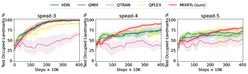
Figure 3: Median test occupied landmarks % across different numbers of agents in the Spread environment.

TABLE III: The number of parameters needs to be learned for different algorithms on different scenarios.

Method	3m	8m	2s3z	5m_vs_6m	3s5z	8m_vs_9m	MMM2	6h_vs_8z
VDN	$28,297$	$32,462$	$31,883$	$30,412$	$35,534$	$32,911$	$39,250$	$32,206$
QMIX	$46,058$	$83,663$	$67,628$	$61,933$	$95,951$	$86,224$	$124,179$	$73,871$
QTRAN	$58,495$	$79,860$	$72,021$	$68,102$	$89,076$	$82,097$	$107,904$	$76,020$
QPLEX	$275,669$	$587,144$	$447,491$	$404,164$	$688,520$	$615,241$	$955,704$	$508,764$
MIXRTs (ours)	$20,880$	$37,040$	$34,448$	$28,752$	$48,560$	$38,592$	$62,736$	$35,440$

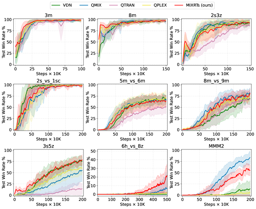
Figure 4: Median test win rates % for easy, hard and super-hard scenarios of SMAC.

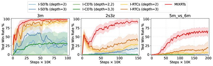
Figure 5: Comparison of I-SDTs, I-CDTs, I-RTCs and MIXRTs with different depths.

During training time, all agents are credited with defeating all enemy units within a limited time after an episode, and the target network is updated once after training every $200$ episodes. We pause the training process for every $5000$ training timesteps and test the win rate of each algorithm for $32$ episodes with the greedy action selection in a decentralized execution manner. All the results are averaged over $8$ runs with different seeds and are displayed in the style of $mean\pm std$. Our model runs from $1$ hour to $15$ hours per task with an NVIDIA RTX 3080TI GPU and an Intel i9-12900k CPU, depending on the complexity and the length of the episode on each scenario.

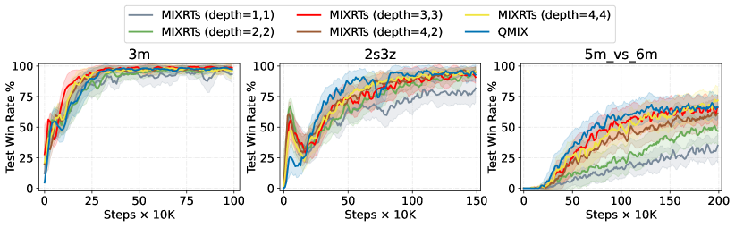
(a) Comparison of different depths on different scenarios.

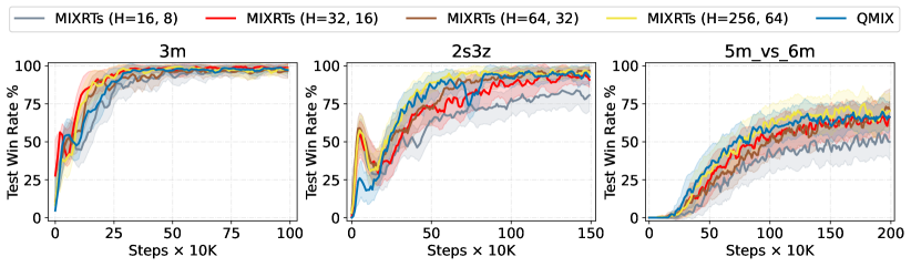
(b) Comparison of different ensemble sizes on different scenarios.

Figure 6: The effect of MIXRTs on performance with respect to the depth and the number of ensemble trees.

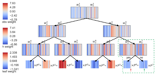
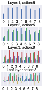
Figure 7: Heatmap visualization of the learned filters and action distributions for each layer. (a) Heatmap visualization of the learned filters in the learned RTCs of depth $3$. The weights of each non-leaf node features contain the current observations (left) and the historical records (right), respectively. The leaf nodes indicate the magnitude of the different action distributions. (b) Actions probability distribution of the nodes of the RTCs with a given observation, where each node is distinguished by a different color bar.

5.3 Performance Comparison

Performance comparison in MPE. We first run the experiments on three specifically tailored Spread tasks. As shown in Fig. 3, our method achieves competitive performance compared to baselines, demonstrating its efficiency across a range of scenarios. In the standard task configuration involving $3$ agents, most algorithms are successful in learning effective policies that result in covering on average $95\%$ of the landmarks, with the exception of QPLEX. Notably, in scenarios with an increased complexity, featuring $4$ or $5$ agents, MIXRTs demonstrates superior performance in later iterations, achieving a consistent strategy that successfully covers $80\%$ to $90\%$ of the landmarks within $4M$ steps. In contrast, other algorithms display significant performance volatility. This suggests that the deployment of a linear structural tree in policy learning is more conducive to consistently optimal strategy, i.e., each agent is tasked with occupying a distinct landmark.

Performance comparison in SMAC. First, we validate MIXRTs on a range of easy scenarios. As shown in Fig. 4, compared to VDN, QMIX, QTRAN, and QPLEX methods, MIXRTs achieves competitive performance with a slightly faster learning process. On the homogeneous scenarios (e.g., 3m and 8m), MIXRTs performs slightly higher performance during the early learning stage. The baselines obtain a sub-optimal strategy with a slightly larger variance in win rates than the MIXRTs. QTRAN performs not well in these comparative experiments, which may suffer from the relaxations in practice impeding its precise updating [34]. Especially in the heterogeneous 2s3z map, the MIXRTs still obtain a competitive performance whose win percentage is near to QMIX and QPLEX, but slightly higher than VDN and QTRAN, which may benefit from the efficient value decomposition by the lightweight inference.

Next, we test the performance of different algorithms on the hard and super-hard scenarios. Fig. 4 illustrates that MIXRTs consistently achieves performance close to the best baseline on different challenging scenarios, and even exceed it on 6h_vs_8z. For three hard scenarios, MIXRTs obtains slightly superior performance compared to other baselines, underscoring its ability to strike an optimal balance between interpretability and cooperative learning performance. Moreover, we compare the performance of different mixing architectures in these scenarios, as shown in Table IV. The results show that the factorization employed within the mixing trees yields a more effective computation of joint action values than VDN and QTRAN. For super hard tasks 6h_vs_8z and MMM2, MIXRTs can search for workable strategies with stable updates compared to most baselines, indicating that our lightweight inference and ensemble structure can improve the learning efficiency and stability on the asymmetric scenarios. To summarize, MIXRTs achieves competitive performance and stable learning behavior while retaining the concise learning architecture with better interpretability.

TABLE IV: Test win rates % of different mixing architectures in hard scenarios, where the methods are named individual function + mixing networks.

Method	5m_vs_6m	3s5z	8m_vs_9m
RNN + VDN Net	${73.95}_{\pm 8.41}$	${82.03}_{\pm 8.11}$	${75.78}_{\pm 14.01}$
RNN + QTRAN Net	${55.46}_{\pm 11.26}$	${17.96}_{\pm 14.31}$	${71.09}_{\pm 17.18}$
RNN + Mixing Trees	${69.17}_{\pm 15.38}$	${87.89}_{\pm 5.04}$	${78.90}_{\pm 10.39}$
RTCs + Mixing Trees	${71.87}_{\pm 12.73}$	${83.98}_{\pm 11.79}$	${84.76}_{\pm 9.16}$

In addition, we also analyze the simplicity of MIXRTs in terms of the number of parameters for the above baselines, which depends mainly on the observation size and the number of agents for different scenarios. As shown in Table III, compared to QMIX, QTRAN, and QPLEX, the parameters that need to be learned for VDN are fewer, since there is no mixing network to represent the state-value function. Since each layer of MIXRTs is represented linearly, the number of parameters increases linearly with the depth of the tree. When the depth of the RTCs is set to $3$, compared to QMIX, QTRAN, and QPLEX, the number of parameters of MIXRTs is reduced by more than $49\%$, whereas it retains competitive performance. With the simplicity of the model, we can more easily understand the critical features and the decision process via lightweight inference, which strikes a better balance between performance and interpretability.

Performance comparison with representative interpretable models based on the tree structure. We evaluate the learning performance of RTCs over the individual SDTs and CDTs methods on both easy and hard scenarios. As shown in Fig. 5, I-RTCs constantly and significantly outperforms I-SDTs and I-CDTs in performance and stability for all the tasks. I-RTCs obtains better performance by combining high-dimensional features mapped from observations with historical action-observation values as input, where adding recurrency information could better capture feature information in complex tasks, especially in non-stationary multi-agent tasks. In terms of stability, I-RTCs performs more stably than SDTs and CDTs, its ensemble mechanism can stabilize the training. Compared to the existing interpretable tree-based methods, MIXRTs outperforms I-SDTs, I-CDTs, and I-RTCs as it shows the advantages of learning a centralized but factored centralized joint action-observation value, especially its lightweight inference architecture.

Generally, deeper trees tend to have more parameters and therefore lay more stress on the interpretability. Here, we further analyze the stability of the decision tree methods with different depths on different scenarios. As shown in Fig. 5, I-SDTs, I-CDTs, and I-RTCs learn faster and perform better as the depth of the tree increases. Note that we utilize the ensemble tree structure and the advanced recurrent technique for I-RTCs, yielding better performance and usually being less sensitive to tree depth than I-SDTs and I-CDTs. From the comparisons, MIXRTs yields substantially better results than other trees. The reason might be the effective approximating ability of MIXRTs in the sophisticated relationship between $Q_{i}$ and $Q_{tot}$ with the mixing trees module to capture different features in sub-spaces.

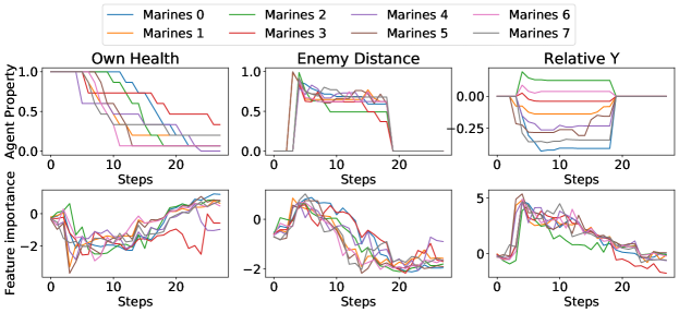
(a) Comparison of feature importance for MIXRTs on 8m.

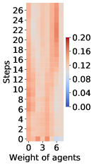
(b) Agent weight heatmap on 8m.

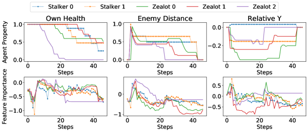
(c) Comparison of feature importance for MIXRTs on 2s3z.

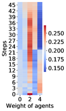
(d) Agent weight heatmap on 2s3z.

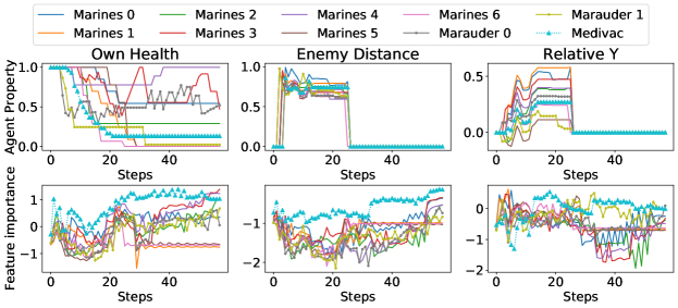
(e) Comparison of feature importance for MIXRTs on MMM2.

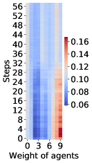
(f) Agent weight heatmap on MMM2

Figure 8: Feature importance and assigned weights of $Q$-values. With the number of steps increases, features importance within the line graph varies correlating to the properties of relevant agents. In the heatmaps, horizontal and vertical ordination indicate the agent-id and steps, respectively.

Sensetivity analysis. In addition, we analyze how sensitive MIXRTs is to the effect of tree depth and the number of ensemble trees on performance. Here, we vary these factors for our experiments to analyze the sensitivity of performance with respect to the tree depth of the individual RTCs and the mixing trees of MIXRTs. Fig. 6(a) and Fig. 6(b) show the respective effects of the above factors on the performance of MIXRTs. First, we investigate the influence of the individual RTCs and the mixing trees with different depths on three scenarios. Fig. 6(a) displays that the performance of MIXRTs will improve as the depth of the individual RTCs and the mixing of RTCs appropriately increases. A greater depth allows MIXRTs to produce more fine-grained behaviors and hence leads to better model performance. However, the improved performance comes at the trade-off of losing its interpretability. Generally, a moderate depth (e.g., depth=3, 3) setting can obtain a competitive performance, where the former $3$ and the latter $3$ represent the depth of the individual action-value RTCs and mixing RTCs of MIXRTs with depth=$3,3$, respectively. Further, we study the effect of the number of ensemble trees on performance. Fig. 6(b) indicates that the tree model shows a clear tendency to be unstable when the number of ensemble trees is small. With moderate values (e.g., $H=32\sim 64$), the tree usually converges quickly and obtains better performance. It shows that the setting with a moderate depth and number of ensemble trees can achieve promising performance while retaining the simplicity and interpretability of the model. For this reason, we chose moderate parameters that are trade-offs between the two, while maintaining a lower amount of parameters comparable to the baselines that can be found in Table III.

6 Interpretability

The main motivation for this work is to create a model whose behavior is easy to understand, mainly by fully understanding the decision process along the root-to-leaf path and their roles in the team. To display the interpretability afforded by our approach, we describe the structure of RTCs via the learned filters at the inner nodes and present the visualization of the learned probability action distribution. Besides, we present the importance of input features elaborating on how they affect decision making through local features and explore the stability of feature importance. Finally, we give user studies to ensure that the interpretation is consistent with human intuition.

6.1 Explaining Tree Structure.

The essence of RTCs is that a kind of model relies on hierarchical decisions instead of hierarchical features. The neural network generally allows the hierarchical features to learn robust and novel representations of the input space, but it will become difficult to interpret once more than one level is present. Compared to the neural network technique, we can immediately engage with each decision made at a higher level of abstraction, where each branching node of the RTCs directly processes the entire input features. By filtering different weights for each feature at each level of branching nodes of the tree, we can understand which features RTCs considers to assign a particular action distribution to a particular state, and how these features influence actions selected by simply examining all the learned filters along the traversed path between the root and the leaf.

As shown in Fig. 7, we display the structure of the learned RTCs model with a depth of $3$ for each agent on a 3m map, where the arrows and lines indicate the connections among tree nodes. Each node assigns different weights to each feature by processing the observed state, where a feature with a more intense color (positive: red, negative: blue) means obtaining a higher magnitude of the weight and receiving more focus. Taking the node in the green dotted area as an example, the three features with more intense color are at position $17$ (representing the relationship with the enemy of $\text{id}=2$), at position $14$ (representing whether this enemy is visible or not), and at position $29$ (representing its own health value). As these positive observations with high weights tend to move to the left leaf, it is essential to select to attack this enemy in the action distribution (marked with a red arrow). Otherwise, the leaf distributions assign probabilities to actions related to moving westward (marked with a green arrow). This behavior is intuitive, as attacking an enemy can bring higher rewards when it has a better chance of survival. Therefore, depending on the choice generated by the activation function, the selected nodes focus on the values of different branching decisions, including action and feature weights.

To understand how a specific state observation influences a particular action distribution, we visualize the decision route from the root to the chosen leaf node in RTCs with the input state. For a given observation, we also provide the action probability distribution for each layer, which is an inherent explanation not provided by the DNNs’ paradigm. As shown in Fig. 7, we can receive the action probability distribution from each layer. Each node outputs a probability distribution with feature vectors, and the selected action depends on the probability linearly combined with the action distribution of each leaf node. From Fig. 7, we can find which features obtain more attention at each layer and how the features affect the action probability distribution. A detailed description is deferred to S. 1 in Supplementary Materials.

TABLE V: Perturbation tests the win rate of MIXRTs. To quantify the interpretation, we use the trained model to calculate the important features in each step via Eq. (12). Then, we mask a varying percentage of least and most important features with zeros for each step and redo the decision making.

Least important data	3m	2s3z	5m_vs_6m	Most important data	3m	2s3z	5m_vs_6m
Masking 0%	${100.00}_{\pm 0.00}$	${100.00}_{\pm 0.00}$	${63.37}_{\pm 2.10}$	Masking 0%	${100.00}_{\pm 0.00}$	${100.00}_{\pm 0.00}$	${63.37}_{\pm 2.10}$
Masking 5%	${100.00}_{\pm 0.00}$	${100.00}_{\pm 0.00}$	${48.95}_{\pm 1.72}$	Masking 5%	${83.48}_{\pm 1.35}$	${93.87}_{\pm 1.18}$	${13.37}_{\pm 3.78}$
Masking 10%	${96.77}_{\pm 1.74}$	${100.00}_{\pm 0.00}$	${41.75}_{\pm 2.57}$	Masking 10%	${63.78}_{\pm 3.89}$	${41.19}_{\pm 0.73}$	${0.00}_{\pm 0.00}$
Masking 20%	${82.19}_{\pm 1.46}$	${70.96}_{\pm 5.26}$	${15.53}_{\pm 3.24}$	Masking 20%	${12.90}_{\pm 1.51}$	${3.22}_{\pm 2.64}$	${0.00}_{\pm 0.00}$
Masking 30%	${48.38}_{\pm 4.15}$	${46.67}_{\pm 3.19}$	${0.00}_{\pm 0.00}$	Masking 30%	${0.00}_{\pm 0.00}$	${0.00}_{\pm 0.00}$	${0.00}_{\pm 0.00}$

6.2 Feature Importance

There are several ways of implementing feature importance assignments on SDTs [31]. However, the data point is more susceptible to being perturbed since it is less confident of remaining in the original when there are multiple boundaries for partitioning the space. We utilize decision confidence as a weight for assigning feature importance, which can be positively correlated with the distance from the instance to the decision boundary to relieve the above effects. Therefore, similar to Eq. (5), we weight the confidence probability of reaching the deepest non-leaf level node $j$ as $P^{j}(o_{i}^{t},h_{i}^{t-1})$. Then, the feature importance can be expressed by multiplying the confidence value with each decision node as

$$I(o_{i}^{t})=\sum_{j}P^{j}(o_{i}^{t},h_{i}^{t-1})w^{j}_{o}.$$ (12)

Feature importance analysis. After obtaining learned RTCs, we evaluated the feature importance of agents on different maps with Eq. (12). we select three feature properties of the agent to indicate their importance and display the weight of individual credit assignment across different episodes, including the agent’s own health, enemy distance, and relative Y properties. We analyze these properties on three different maps, and the results are shown in Figs. 8(a), 8(c), and 8(e), respectively. The horizontal coordinate represents the number of steps in the episode, and two vertical coordinates represent the corresponding value of the agent property and feature importance, respectively. Meanwhile, we visualize the weights $W_{i}$ for each agent $i$ on each scenario, and the weight heatmaps are shown in Figs. 8(b), 8(d) and 8(f). In the attention heatmaps, the steps increase from bottom to top, and the horizontal ordination indicates the agent id.

For 8m, it is essential to achieve a victory that the agents avoid being killed and pay more attention to firepower for killing the enemies. From Fig. 8(a), we observe that allies have similar feature importance on the same attribute. It is worth noting that when an enemy is killed in combat, both the importance of the distance to this enemy and its relative Y will decrease. It suggests that RTCs can capture the skills for accomplishing tasks and generate coping actions when the environment changes. In addition, as shown in Fig. 8(b), we can find that each agent has almost equal attention weights, indicating that each allied Marine plays a similar role on the homogeneous scenario, and MIXRTs almost equally divides $Q_{tot}$ for each agent. MIXRTs performs well with the refined mixing trees since it adjusts the weights of $Q_{i}$ with a minor difference. For the 2s3z scenario, we can find that Stalkers and Zealots each have similar feature importance at different steps, which might be sourced from the fact that they all focus on their health and play an equally important role in the battle. Besides, when the health value of the Zealot $2$ is $0$, we also find that it achieves strongly negative importance with blue shades as shown in Fig. 8(d), where the agent does not play an active role in battle since it is killed. It is of interest that the drastic change in the weight of the agents on 2s3z since the replacement of Zealot $2$ by Zealot $0$ after its death in battle, coinciding with a rise in the importance of distance and health. Furthermore, we notice that different types of soldiers have different sensitivity to features. For example, Medivac (agent $9$ in Fig. 8(f)) receives more attention during the early stages of the battle, which may be attributed to their different roles involved in combat. In summary, by analyzing the feature importance, we receive meaningful implicit knowledge of the tasks, which can facilitate human understanding of why particular feature importance leads to a certain action.

Perturbing important features. Due to the large number of features involved in the decision-making process, we mask certain features by degradation of performance to measure their importance. For a trained MIXRTs, we first calculate the feature importance at each step through the nodes. Then, we evaluates performance by substituting the most and least important features with zeros, implying that the corresponding nodes in the tree structure are not involved in the calculation. The performance results of win rate are presented in Table V. When perturbing a portion of unimportant features remains relatively stable in performance, which suggests that the critical decision-making process does not heavily rely on the full set of features. Conversely, the perturbing of features deemed important leads to a marked degradation in performance, affirming their significance in the decision-making process. Furthermore, with an increase in the proportion of masked features, the win rate of perturbing critical features precipitously declines to zero, while vice versa does not. This demonstrates the effectiveness of MIXRTs in evaluating the importance of features and allows for the exclusion of a portion of features that are inconsequential to the decision-making process.

6.3 Stability on Feature Importance

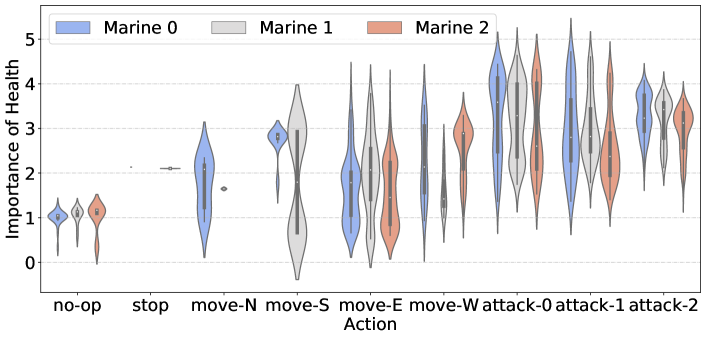
(a) The violin plot of feature importance on 3m.

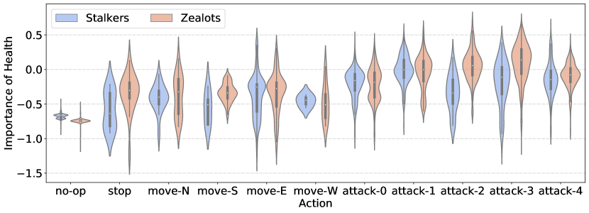
(b) The violin plot of feature importance on 2s3z.

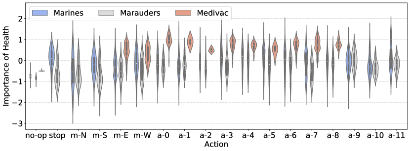
(c) The violin plot of feature importance on MMM2.

Figure 9: Depicting the stability on fitted MIXRTs through violin plots. Broad sections of the plot denote a higher density distribution, while narrow portions imply a less dense distribution.

The stability of the interpretable model is an important factor reflecting the reliability. To further study the stability, we take a deeper look into MIXRTs itself regarding the assigned feature importance and the action distributions. We conduct analyses with the violin plot to study action distribution among several episodes. With the violin plot, it would be beneficial for us to immediately identify the median feature importance size without having to visually estimate it by integrating the density, which can help us receive strictly more information and analyze the stability of feature importance. We hope this can alleviate the differences in action distributions caused by the different initial states of each episode. As shown in Fig. 9, we select the health property of the agents to indicate the correlation between the underlying action distribution and the assigned feature importance over $32$ episodes. The horizontal coordinate and the vertical coordinate represent the selected action and the importance of the health of the agent itself.

For the 3m scenario, it requires the three allied agents to pay more attention to firepower to kill the enemies with fewer casualties. As shown in Fig. 9, we can observe that the three allies own similar importance among all the actions, which aligns with the common knowledge that homogeneous agents play the same important role during the battles. Besides, we also find that they pay more attention to selecting attack actions, which may mean that it can bring more positive rewards to ensure victory than taking the other actions in this easy homogeneous agent environment. From Figs. 9(b) and 9(c), considerable differences can also be spotted over $32$ episodes on the heterogeneous scenarios 2s3z and MMM2, even though MIXRTs has captured similar skills to win. For the 2s3z scenario, we see Zealots obtaining a higher importance of health than Stalkers, which may require a better winning strategy where Zealots agents serve at the front of combat, killing enemies one after another while protecting the Stalkers to kite the enemy around the map. Furthermore, we notice that similar interesting findings also exist on the MMM2 scenario. For example, Medivac, as a healer unit, receives more attention than other kinds of agents during the battle. This could lead the cooperative team to defeat the enemies more since Medivac uses healing actions to improve the health of its allies. It consistent with the above analysis in Section 6.2.

Overall, the importance of health is slightly higher when the agents are in attacking status than in moving status, and is significantly higher than when they are not operating. Since on most occasions when the agents are attacking, they are also being attacked, the importance of health is more intense. Meanwhile, agents who are killed receive the negative importance of health with a small interquartile range. As far as the stability is concerned, the non-operation of agents also maintains a steady state in the model since most of them own a health value of $0$. In summary, even though the different initialized environments change, we could still find the implicit knowledge from MIXRTs by analyzing the feature importance over several episodes.

6.4 Case Study

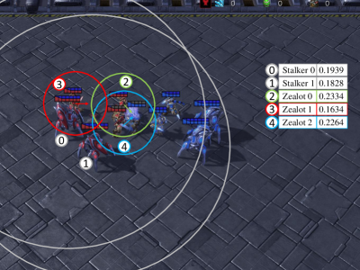
(a) 2s3z (step=10)

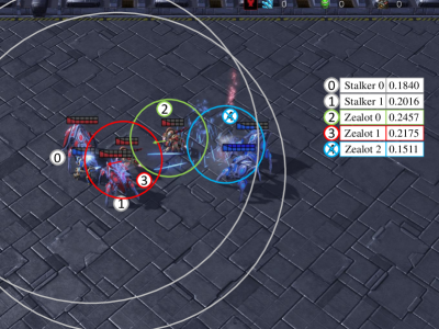
(b) 2s3z (step=27)

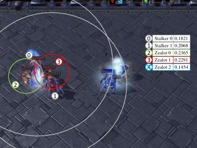
(c) 2s3z (step=34)

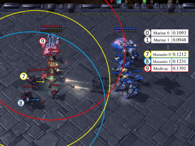
(d) MMM2 (step=7)

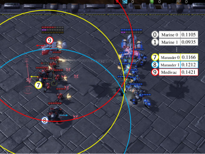
(e) MMM2 (step=12)

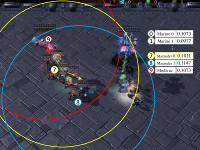
(f) MMM2 (step=35)

Figure 10: Visualization of the evaluation for MIXRTs on 2s3z and MMM2 scenarios in SMAC (time step goes from left to right). For each task, the credit assignment weights for each agent are displayed at the top-right of each frame. The arrow and the colored circle indicate the direction that each moving agent is facing and the central attack range, respectively. For the 2s3z scenario, the agents will receive higher credit when they focus on killing the enemy within its range of attacking, which implies the credits reflecting their contributions to the team. They learn a skill-winning strategy that they collectively wall off the choke point to block enemy attacks from different directions as shown in frames (a) and (b). For the MMM2 scenario, the assigned credit for each unit indicates the important role that Medivac receives the highest credit during the early stage of the battle since it can heal the allied units, and Marauders receive higher credit than Marines for their high damage.

To further show the interpretability of MIXRTs, we present the keyframes on these episodes during the testing stage in Fig. 10. As seen from Fig. 10(a), during the initial stage (step=$10$) of 2s3z, Zealot $2$ and Zealot $0$ are participating in the battle, and meanwhile, Zealot $1$ drops teammates. It can be understood that Zealot $2$ and Zealot $0$ make contributions to the team and Zealot $1$ does not contribute to the team. Their credit assignment weights $0.23344$, $0.22639$, and $0.16338$ correctly catch the manner of Zealot $0$, Zealot $2$ and Zealot $1$, respectively. When Zealot $2$ was killed as shown in Fig. 10(b), its credit assignment weight also quickly dropped to the lowest team level, and meanwhile, its allies’ weight increased. During the battle process, both Stalkers capture high-level skills with stable credit assignment weights when the team is in a combat tactic, where they nearly always attack enemies behind teammates for getting the utmost out of their long-range attack attributes. Besides, Zealot $0$ and Zealot $1$ focus on killing the enemy as they obtain higher credit at step $34$. As a result, Zealot $0$ and Zealot $1$ contribute more than others and therefore their credits are greater, which implies that the credits reflect contribution to the team. For the MMM2 scenario, we find an interesting strategy to win the battle that the being attacked Medivac will retreat out of being attacked range while the allies move forward to prevent Medivac from being attacked. Its credit assignment weight correctly catches the important role of its team with the highest credit during the early stage of the battle. Besides, Marauders (Agents $7$ and $8$) receive higher credit for their high damage, they get healing blood from the Medivac agent as shown in Figs. 10(f). In a summary, MIXRTs can help us understand the behaviors of agents and their contribution to the team via linear credit assignments on different complicated scenarios.

6.5 User Study

Our final evaluation investigates the effect of the interpretability provided by MIXRTs for non-experts. Following Silva et al. [28, 55], we have similarly conducted a user study, showing participants trained policies on SMAC scenarios. They are tasked with identifying whether these agents’ credit assignments are reasonable given a set of observation inputs and keyframes (similar to Fig.  10). We compare the credit assignment rationality of MIXRTs, VDN, and QMIX. We then present our results to $20$ participants, instructing each of them to assign a $1\sim 5$ helpfulness score with a set of Likert scales to every result. The Likert scale guideline is provided on each score for justified scoring as follow

• Score $1$ for misleading credits that impair the decision-making process.

• Score $2$ for uninformative credits that neither aid nor hinder human understanding.

• Score $3$ for deviated but somewhat related credits that provide slight assistance.

• Score $4$ for strongly related keyframes but slightly inaccurate, helpful.

• Score $5$ for well-aligned credits that contain all information in combat, exceptionally helpful.

Each participant is required to observe the keyframes without knowing which method produced the policy, ensuring full fairness. For each method, we sample $22$ frames and time them separately.

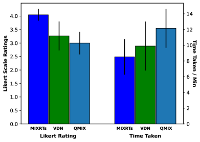
Figure 11: Results from our user study. Higher Likert ratings are better, and lower time taken is better.

Results of our user study are shown in Fig. 11. Consistent with intuition and previous metrics, human evaluators reveal a positive estimation of $4.0485$ helpfulness rating. The rating indicates our MIXRTs generally offers a moderate enhancement to interpretability. Notably, this result substantially outperforms QMIX’s $2.9979$ helpfulness and VDN’s $3.2640$ helpfulness, both of which means vague and deviate related content. We conduct an ANOVA, which yields that $F(2,57)=33.40,p<0.0001$ for the Likert scale ratings. It indicates that different mixers significantly effect the interpretability and usability of credit assignment. A Tukey’s HSD post-hoc test shows that MIXRTs vs. QMIX is $t=10.26,p<0.0001$, and MIXRTs vs. VDN is $t=7.67,p<0.0001$. We also test participants’ time in Fig. 11 and show that MIXRTs takes the least amount of time compared to the other methods. An interesting observation from the study participants is that they would have abandoned the task if what they knew was the credit generated by QMIX. These results support the hypothesis that our model significantly outperforms other approaches in reducing human frustration and improving interpretability. These empirical insights lend robust support to the supposition that our proposed model markedly excels in diminishing human frustration and enhancing interpretability.

7 Conclusion

This paper presented MIXRTs, a novel interpretable MARL mixing architecture based on the SDTs with recurrent structure. MIXRTs allows end-to-end training in a centralized fashion and learns to linearly factorize a joint action-value function for executing decentralized policies. The empirical results show that MIXRTs not only enjoy good model interpretability and scalability while maintaining competitive learning performance. Our approach captures the implicit knowledge of the challenging tasks with a transparent model and facilitates understanding of the learned domain knowledge and how input states influence decisions, which paves the application process in high-stake domains. Our linear mixing component demonstrates the possibility to produce the credit assignment to analyze what role each agent plays in its allies. Our work motivates future work toward building more interpretable and explainable multi-agent systems. In future work, we will try to analyze the evaluation process, and approach a more trustworthy interpretation of the feature importance estimation, aiming at further minimizing the cost of human effort for understanding the decision process.

References

- [1] O. Vinyals, I. Babuschkin, W. M. Czarnecki, M. Mathieu, A. Dudzik, J. Chung, D. H. Choi, R. Powell, T. Ewalds, P. Georgiev et al., “Grandmaster level in StarCraft II using multi-agent reinforcement learning,” Nature, vol. 575, no. 7782, pp. 350–354, 2019.
- [2] P. Sunehag, G. Lever, A. Gruslys, W. M. Czarnecki, V. Zambaldi, M. Jaderberg, M. Lanctot, N. Sonnerat, J. Z. Leibo, K. Tuyls et al., “Value-decomposition networks for cooperative multi-agent learning based on team reward,” in Proceedings of the International Conference on Autonomous Agents and MultiAgent Systems, 2018, pp. 2085–2087.
- [3] T. Rashid, M. Samvelyan, C. S. de Witt, G. Farquhar, J. N. Foerster, and S. Whiteson, “QMIX: Monotonic value function factorisation for deep multi-agent reinforcement learning,” in Proceedings of the International Conference on Machine Learning, vol. 80, 2018, pp. 4295–4304.
- [4] C. Yu, X. Wang, X. Xu, M. Zhang, H. Ge, J. Ren, L. Sun, B. Chen, and G. Tan, “Distributed multiagent coordinated learning for autonomous driving in highways based on dynamic coordination graphs,” IEEE Transactions on Intelligent Transportation Systems, vol. 21, no. 2, pp. 735–748, 2019.
- [5] B. R. Kiran, I. Sobh, V. Talpaert, P. Mannion, A. A. Al Sallab, S. Yogamani, and P. Pérez, “Deep reinforcement learning for autonomous driving: A survey,” IEEE Transactions on Intelligent Transportation Systems, vol. 23, no. 6, pp. 4909–4926, 2021.
- [6] I.-J. Liu, Z. Ren, R. A. Yeh, and A. G. Schwing, “Semantic tracklets: An object-centric representation for visual multi-agent reinforcement learning,” in Proceedings of the IEEE/RSJ International Conference on Intelligent Robots and Systems, 2021, pp. 5603–5610.
- [7] J. Kober, J. A. Bagnell, and J. Peters, “Reinforcement learning in robotics: A survey,” The International Journal of Robotics Research, vol. 32, no. 11, pp. 1238–1274, 2013.
- [8] N. Topin, S. Milani, F. Fang, and M. Veloso, “Iterative bounding MDPs: Learning interpretable policies via non-interpretable methods,” in Proceedings of the AAAI Conference on Artificial Intelligence, vol. 35, no. 11, 2021, pp. 9923–9931.
- [9] H. Liu, R. Wang, S. Shan, and X. Chen, “What is a tabby? Interpretable model decisions by learning attribute-based classification criteria,” IEEE Transactions on Pattern Analysis and Machine Intelligence, vol. 43, no. 5, pp. 1791–1807, 2019.
- [10] B. Zhou, D. Bau, A. Oliva, and A. Torralba, “Interpreting deep visual representations via network dissection,” IEEE Transactions on Pattern Analysis and Machine Intelligence, vol. 41, no. 9, pp. 2131–2145, 2018.
- [11] Z. C. Lipton, “The mythos of model interpretability,” Queue, vol. 16, no. 3, pp. 31–57, 2018.
- [12] E. Tjoa and C. Guan, “A survey on explainable artificial intelligence (XAI): Toward medical XAI,” IEEE Transactions on Neural Networks and Learning Systems, vol. 32, no. 11, pp. 4793–4813, 2020.
- [13] C. Rudin, “Stop explaining black box machine learning models for high stakes decisions and use interpretable models instead,” Nature Machine Intelligence, vol. 1, no. 5, pp. 206–215, 2019.
- [14] C. Rudin, C. Chen, Z. Chen, H. Huang, L. Semenova, and C. Zhong, “Interpretable machine learning: Fundamental principles and 10 grand challenges,” Statistics Surveys, vol. 16, pp. 1–85, 2022.
- [15] X. Xu, Z. Wang, C. Deng, H. Yuan, and S. Ji, “Towards improved and interpretable deep metric learning via attentive grouping,” IEEE Transactions on Pattern Analysis and Machine Intelligence, vol. 45, no. 1, pp. 1189–1200, 2022.
- [16] Q. Cao, X. Liang, B. Li, and L. Lin, “Interpretable visual question answering by reasoning on dependency trees,” IEEE Transactions on Pattern Analysis and Machine Intelligence, vol. 43, no. 3, pp. 887–901, 2019.
- [17] M. Natarajan and M. Gombolay, “Effects of anthropomorphism and accountability on trust in human robot interaction,” in Proceedings of the ACM/IEEE International Conference on Human-Robot Interaction, 2020, pp. 33–42.
- [18] E. Puiutta and E. Veith, “Explainable reinforcement learning: A survey,” in Proceedings of the International Cross-Domain Conference for Machine Learning and Knowledge Extraction, 2020, pp. 77–95.
- [19] W. Shi, G. Huang, S. Song, Z. Wang, T. Lin, and C. Wu, “Self-supervised discovering of interpretable features for reinforcement learning,” IEEE Transactions on Pattern Analysis and Machine Intelligence, vol. 44, no. 5, pp. 2712–2724, 2020.
- [20] T. Zahavy, N. Ben-Zrihem, and S. Mannor, “Graying the black box: Understanding DQNs,” in Proceedings of the International Conference on Machine Learning, vol. 48, 2016, pp. 1899–1908.
- [21] A. Verma, “Verifiable and interpretable reinforcement learning through program synthesis,” in Proceedings of the AAAI Conference on Artificial Intelligence, 2019, pp. 9902–9903.
- [22] Z. Jiang and S. Luo, “Neural logic reinforcement learning,” in Proceedings of the International Conference on Machine Learning, vol. 97, 2019, pp. 3110–3119.
- [23] W. Shi, G. Huang, S. Song, and C. Wu, “Temporal-spatial causal interpretations for vision-based reinforcement learning,” IEEE Transactions on Pattern Analysis and Machine Intelligence, vol. 44, no. 12, pp. 10 222–10 235, 2021.
- [24] D. Silver, A. Huang, C. J. Maddison, A. Guez, L. Sifre, G. Van Den Driessche, J. Schrittwieser, I. Antonoglou, V. Panneershelvam, M. Lanctot et al., “Mastering the game of Go with deep neural networks and tree search,” Nature, vol. 529, no. 7587, pp. 484–489, 2016.
- [25] W.-Y. Loh, “Classification and regression trees,” Wiley Interdisciplinary Reviews: Data Mining and Knowledge Discovery, vol. 1, no. 1, pp. 14–23, 2011.
- [26] L. Breiman, “Random forests,” Machine Learning, vol. 45, no. 1, pp. 5–32, 2001.
- [27] N. Frosst and G. Hinton, “Distilling a neural network into a soft decision tree,” arXiv preprint arXiv:1711.09784, 2017.
- [28] A. Silva, M. Gombolay, T. Killian, I. Jimenez, and S.-H. Son, “Optimization methods for interpretable differentiable decision trees applied to reinforcement learning,” in Proceedings of the International Conference on Artificial Intelligence and Statistics, vol. 108, 2020, pp. 1855–1865.
- [29] A. Suárez and J. F. Lutsko, “Globally optimal fuzzy decision trees for classification and regression,” IEEE Transactions on Pattern Analysis and Machine Intelligence, vol. 21, no. 12, pp. 1297–1311, 1999.
- [30] Y. Coppens, K. Efthymiadis, T. Lenaerts, A. Nowé, T. Miller, R. Weber, and D. Magazzeni, “Distilling deep reinforcement learning policies in soft decision trees,” in Proceedings of the IJCAI Workshop on Explainable Artificial Intelligence, 2019, pp. 1–6.
- [31] Z. Ding, P. Hernandez-Leal, G. W. Ding, C. Li, and R. Huang, “CDT: Cascading decision trees for explainable reinforcement learning,” arXiv preprint arXiv:2011.07553, 2020.
- [32] G. Brockman, V. Cheung, L. Pettersson, J. Schneider, J. Schulman, J. Tang, and W. Zaremba, “OpenAI Gym,” arXiv preprint arXiv:1606.01540, 2016.
- [33] M. Samvelyan, T. Rashid, C. S. De Witt, G. Farquhar, N. Nardelli, T. G. Rudner, C.-M. Hung, P. H. Torr, J. Foerster, and S. Whiteson, “The starcraft multi-agent challenge,” in Proceedings of the International Joint Conference on Autonomous Agents and MultiAgent Systems, 2019, pp. 2186–2188.
- [34] J. Wang, Z. Ren, T. Liu, Y. Yu, and C. Zhang, “QPLEX: Duplex dueling multi-agent Q-learning,” in Proceedings of the International Conference on Learning Representations, 2021.
- [35] F. A. Oliehoek and C. Amato, A concise introduction to decentralized POMDPs. SpringerBriefs in Intelligent Systems. Springer, 2016.
- [36] C. J. Watkins and P. Dayan, “Q-learning,” Machine Learning, vol. 8, no. 3, pp. 279–292, 1992.
- [37] K. Son, D. Kim, W. J. Kang, D. E. Hostallero, and Y. Yi, “QTRAN: Learning to factorize with transformation for cooperative multi-agent reinforcement learning,” in Proceedings of the International Conference on Machine Learning, vol. 97, 2019, pp. 5887–5896.
- [38] L. Pan, T. Rashid, B. Peng, L. Huang, and S. Whiteson, “Regularized softmax deep multi-agent Q-learning,” in Proceedings of the Advances in Neural Information Processing Systems, vol. 34, 2021, pp. 1365–1377.
- [39] V. Mnih, K. Kavukcuoglu, D. Silver, A. A. Rusu, J. Veness, M. G. Bellemare, A. Graves, M. Riedmiller, A. K. Fidjeland, G. Ostrovski et al., “Human-level control through deep reinforcement learning,” Nature, vol. 518, no. 7540, pp. 529–533, 2015.
- [40] O. Irsoy, O. T. Yıldız, and E. Alpaydın, “Soft decision trees,” in Proceedings of the International Conference on Pattern Recognition, 2012, pp. 1819–1822.
- [41] D. Laptev and J. M. Buhmann, “Convolutional decision trees for feature learning and segmentation,” in Proceedings of the German Conference on Pattern Recognition, 2014, pp. 95–106.
- [42] A. M. Roth, N. Topin, P. Jamshidi, and M. Veloso, “Conservative Q-improvement: Reinforcement learning for an interpretable decision-tree policy,” arXiv preprint arXiv:1907.01180, 2019.
- [43] A. Pace, A. Chan, and M. van der Schaar, “POETREE: Interpretable policy learning with adaptive decision trees,” in Proceedings of the International Conference on Learning Representations, 2021, pp. 1–28.
- [44] M. Tan, “Multi-agent reinforcement learning: Independent vs cooperative agents,” in Proceedings of the International Conference on Machine Learning, 1993, pp. 330–337.
- [45] F. A. Oliehoek, M. T. Spaan, and N. Vlassis, “Optimal and approximate Q-value functions for decentralized POMDPs,” Journal of Artificial Intelligence Research, vol. 32, pp. 289–353, 2008.
- [46] L. Kraemer and B. Banerjee, “Multi-agent reinforcement learning as a rehearsal for decentralized planning,” Neurocomputing, vol. 190, pp. 82–94, 2016.
- [47] M. Hausknecht and P. Stone, “Deep recurrent Q-learning for partially observable MDPs,” in Proceedings of the AAAI Fall Symposium on Sequential Decision Making for Intelligent Agents, 2015, pp. 29–37.
- [48] C. Zhang and Y. Ma, Ensemble machine learning: Methods and applications. Springer, 2012.
- [49] H. Hazimeh, N. Ponomareva, P. Mol, Z. Tan, and R. Mazumder, “The tree ensemble layer: Differentiability meets conditional computation,” in Proceedings of the International Conference on Machine Learning, vol. 119, 2020, pp. 4138–4148.
- [50] P. Derbeko, R. El-Yaniv, and R. Meir, “Variance optimized bagging,” in Proceedings of the European Conference on Machine Learning, 2002, pp. 60–72.
- [51] H. van Hasselt, “Double Q-learning,” in Proceedings of the Advances in Neural Information Processing Systems, vol. 23, 2010, pp. 2613–2621.
- [52] H. Van Hasselt, A. Guez, and D. Silver, “Deep reinforcement learning with double Q-learning,” in Proceedings of the AAAI Conference on Artificial Intelligence, vol. 30, no. 1, 2016, pp. 2094–2100.
- [53] R. Lowe, Y. I. Wu, A. Tamar, J. Harb, O. Pieter Abbeel, and I. Mordatch, “Multi-agent actor-critic for mixed cooperative-competitive environments,” in Proceedings of the Advances in Neural Information Processing Systems, vol. 30, 2017.
- [54] A. Tampuu, T. Matiisen, D. Kodelja, I. Kuzovkin, K. Korjus, J. Aru, J. Aru, and R. Vicente, “Multiagent cooperation and competition with deep reinforcement learning,” PloS one, vol. 12, no. 4, pp. 1–15, 2017.
- [55] A. Silva and M. Gombolay, “Encoding human domain knowledge to warm start reinforcement learning,” in Proceedings of the AAAI conference on artificial intelligence, vol. 35, no. 6, 2021, pp. 5042–5050.