A GMOS/IFU Study of Jellyfish Galaxies in Massive Clusters

Abstract

Jellyfish galaxies are an intriguing snapshot of galaxies undergoing ram-pressure stripping (RPS) in dense environments, showing spectacular star-forming knots in their disks and tails. We study the ionized gas properties of five jellyfish galaxies in massive clusters with Gemini GMOS/IFU observations: MACSJ0916-JFG1 ($z=0.330$), MACSJ1752-JFG2 ($z=0.353$), A2744-F0083 ($z=0.303$), MACSJ1258-JFG1 ($z=0.342$), and MACSJ1720-JFG1 ($z=0.383$). BPT diagrams show that various mechanisms (star formation, AGN, or mixed effects) are ionizing gas in these galaxies. Radial velocity distributions of ionized gas seem to follow disk rotation of galaxies, with the appearance of a few high-velocity components in the tails as a sign of RPS. Mean gas velocity dispersion is lower than 50 ${\rm km~{}s^{-1}}$ in most star-forming regions except near AGNs or shock-heated regions, indicating that the ionized gas is dynamically cold. Integrated star formation rates (SFRs) of these galaxies range from $7~{}{\rm M_{\odot}~{}{\rm yr^{-1}}}$ to $35~{}{\rm M_{\odot}~{}{\rm yr^{-1}}}$ and the tail SFRs are from $0.6~{}{\rm M_{\odot}~{}{\rm yr^{-1}}}$ to $16~{}{\rm M_{\odot}~{}{\rm yr^{-1}}}$, which are much higher than those of other jellyfish galaxies in the local universe. These high SFR values imply that RPS triggers intense star formation activity in these extreme jellyfish galaxies. The phase-space diagrams demonstrate that the jellyfish galaxies with higher stellar masses and higher host cluster velocity dispersion are likely to have more enhanced star formation activity. The jellyfish galaxies in this study have similar gas kinematics and dynamical states to those in the local universe, but they show a much higher SFR.

1 Introduction

Environmental effects play an important role in galaxy transformation associated with high-density environments. Most gas-rich galaxies in galaxy groups or clusters evolve by losing their gas content due to various mechanisms: galaxy mergers (Toomre & Toomre, 1972), ram-pressure stripping (RPS; Gunn & Gott, 1972), galaxy harassment (Moore et al., 1996), and starvation (Larson et al., 1980). These external processes remove the gas ingredients for star formation from galaxies and transform late-type galaxies into early-type galaxies in dense environments.

Among these mechanisms, RPS is the interaction between the intracluster medium (ICM) and the interstellar medium (ISM) in galaxies. It has been known as the most efficient mechanism of gas removal from galaxies in cluster environments. When a galaxy moves through the intergalactic space that is filled with hot and diffuse gas, ram pressure applies a force to the gas component in the galaxy towards the direction opposite of the galaxy motion. RPS eventually quenches star formation activity by sweeping out the gas content in galaxies. Since diffuse ICM gas with X-ray emission is frequently observed in galaxy clusters, RPS seems to significantly contribute to the passive evolution of cluster galaxies (Dressler, 1980).

However, some late-type galaxies undergoing RPS are not quiescent but rather show local star-forming regions. Several late-type galaxies under the effect of RPS in Virgo and Coma were found to have a large number of blue and UV-emitting knots or “spur clusters” throughout their disks (Hester et al., 2010; Smith et al., 2010; Yoshida et al., 2012; Lee & Jang, 2016). Interestingly, a post-merger elliptical galaxy in Abell 2670 was revealed to be undergoing RPS and exhibits compact star-forming blobs outside the main body of the galaxy (Sheen et al., 2017). Cluster galaxies with remarkable RPS features like one-sided tails and bright star-forming knots are often called “jellyfish galaxies” (Bekki, 2009; Chung et al., 2009). The presence of young stellar systems in jellyfish galaxies implies that RPS can locally boost the star formation activity in gas-rich galaxies before removing gas completely. Thus, jellyfish galaxies are very interesting and useful targets to investigate the relationship between star formation activity and RPS.

Table 1: Examples of Jellyfish Galaxies (JFGs) at $z>0.1$

Reference	JFGs (Host System)	Redshift	Observing Instruments
Owen et al. (2006)	C153 (A2125)	$z=0.253$	HST/WFPC2, KPNO 4m,
			Gemini/GMOS longslit
			VLA, Chandra
Cortese et al. (2007)	131124$-$012040 (A1689)	$z=0.187$	HST/WFPC2, HST/ACS,
	235144$-$260358 (A2667)	$z=0.227$	VLT/ISAAC, Spitzer/IRAC,
			Spitzer/MIPS, VLA,
			VLT/VIMOS, Keck/LRIS
Owers et al. (2012)	4 JFGs (A2744)	$z=0.29-0.31$	HST/ACS
			AAT/AAOmega
Ebeling et al. (2014)	6 JFGs	$z=0.3-0.5$	HST/ACS
	(37 MACS clusters)
McPartland et al. (2016)	16 JFGs	$z=0.3-0.5$	HST/ACS,
	(63 MACS clusters)		Keck/DEIMOS
Ebeling et al. (2017)	MACSJ0553-JFG1	$z=0.442$	HST/ACS, HST/WFC3,
	(MACSJ0553$-$3342)		Keck/LRIS, Keck/DEIMOS,
			Chandra, GMRT
Boselli et al. (2019)	ID 345 and ID 473 (CGr32)	$z=0.73$	VLT/MUSE, XMM-Newton,
			HST/ACS, Subaru/Suprime-Cam
Kalita & Ebeling (2019)	A1758N_JFG1 (A1758N)	$z=0.273$	Keck/KCWI, Keck/DEIMOS,
			HST/ACS, Chandra
Roman-Oliveira et al. (2019)	70 JFGs (A901/2)	$z=0.165$	GTC/OSIRIS (the OMEGA survey),
			HST/ACS, XMM-Newton
Castignani et al. (2020)	The southern companion of BCG	$z=1.71$	IRAM/NOEMA, HST/ACS
	(SpARCS1049+56)
Durret et al. (2021)	81 JFGs (MACS0717.5$+$3745)	$z=0.546$	HST/ACS
	97 JFGs (22 clusters)	$z=0.2-0.9$	NASA/IPAC Extragalactic Database
Moretti et al. (2022)	13 JFGs (A2744 and A370)	$z=0.3-0.4$	HST/ACS, VLT/MUSE

Recently, observational studies on jellyfish galaxies have utilized integral field spectroscopy (IFS). IFS observations provide both spatial and spectral information, so they are optimal to investigate various physical properties of jellyfish galaxies. For instance, the GAs Stripping Phenomena (GASP) survey observed a large sample of jellyfish galaxies in nearby galaxy clusters using the Multi Unit Spectroscopic Explorer (MUSE) on the Very Large Telescope (VLT) (Poggianti et al., 2017). Studies from the GASP survey found that star-forming knots in jellyfish galaxies are formed in situ with stellar ages younger than 10 Myr, are dynamically cold ($\sigma_{v,{\rm gas}}<40~{}{\rm km~{}s^{-1}}$), and are mostly ionized by photons emitted from young massive stars (Bellhouse et al., 2017, 2019). They obtained a mean star formation rate (SFR) of $\sim 1.8$ $M_{\odot}~{}{\rm yr^{-1}}$ in the disks and $\sim 0.13$ $M_{\odot}~{}{\rm yr^{-1}}$ in the tails of the jellyfish galaxies (Poggianti et al., 2019; Gullieuszik et al., 2020). As a result, the GASP survey has successfully provided a comprehensive view of the star formation activity of jellyfish galaxies in the local universe ($z<0.1$).

However, most IFS studies have been limited to jellyfish galaxies in low-mass clusters ($\sigma_{v,{\rm cl}}\lesssim 1000$ ${\rm km~{}s^{-1}}$) in the local universe ($z<0.1$). Since massive clusters are rare in the nearby universe, jellyfish galaxies in massive clusters have been mostly found at intermediate redshift $(z>0.1)$ and were studied using deep images from the Hubble Space Telescope (HST). Table 1 lists the jellyfish galaxies that have been mainly observed at $z>0.1$ so far. All the observations used HST optical images because such high-resolution images show the dramatic features of jellyfish galaxies very well. Owen et al. (2006) and Cortese et al. (2007) found three disturbed jellyfish galaxies with blue star-forming knots in the multi-band HST optical images and radio images: C153 (Abell 2125; $z=0.253$), 131124-012040 (Abell 1689; $z=0.187$), and 235144-260358 (Abell 2667; $z=0.227$). Owers et al. (2012) studied four jellyfish galaxies with highly asymmetric tails and very bright star-forming knots in the merging cluster Abell 2744, using the HST optical images and AAOmega spectra. Ebeling et al. (2014) and McPartland et al. (2016) performed a systematic search of jellyfish galaxies using the HST images of the Massive Cluster Survey (MACS; Ebeling et al., 2001, 2010) and provided a catalog of 16 jellyfish galaxies in the MACS cluster samples at $z>0.3$ ($\langle M_{\rm tot}\rangle\sim 1.3\times 10^{15}~{}M_{\odot}$). Roman-Oliveira et al. (2019) presented the characteristics of 70 jellyfish galaxies using the OMEGA-OSIRIS survey of a multi-cluster system A901/2. Similarly, Durret et al. (2021) found a total of 178 jellyfish galaxy candidates in 23 clusters from the DAFT/FADA and CLASH surveys.

Among the studies described in Table 1, the IFS observations of jellyfish galaxies at $z>0.1$ are rare except for the three cases. Boselli et al. (2019) detected two massive star-forming galaxies with long gaseous tails in the COSMOS cluster CGr32 ($z=0.73$) using VLT/MUSE. Kalita & Ebeling (2019) studied an extreme jellyfish galaxy, A1758N-JFG1, in the colliding galaxy cluster Abell 1758N ($z=0.28)$ with the Keck Cosmic Web Imager (KCWI). These two studies focused on the resolved kinematics of jellyfish galaxies based on the [O II]$\lambda\lambda 3727,3729$ doublet emission line because their IFS data did not cover the ${\rm H\alpha}$ emission line. Recently, Moretti et al. (2022) presented the properties of 13 jellyfish galaxies in the inner regions of Abell 2744 ($z=0.306$) and Abell 370 ($z=0.375$) using the emission lines of ${\rm H\alpha}$ and [O II]$\lambda\lambda 3727,3729$. Their study suggested that the [O II]/${\rm H\alpha}$ ratio in the tails of their sample galaxies is much higher than those of local jellyfish galaxies, which implies that the stripped gas might have low gas density or interact with the ICM.

In this study, we investigate the physical properties of jellyfish galaxies in massive clusters using the integral field unit (IFU) instrument on the Gemini Multi-Object Spectrograph (GMOS). The 8-m Gemini telescope is suitable for observing jellyfish galaxies at intermediate redshift in terms of its light-gathering power and field of view (FOV). We carry out emission line analyses of the GMOS/IFU data of jellyfish galaxies, which includes the ${\rm H\alpha}$ line. Using the ${\rm H\alpha}$-derived SFRs of jellyfish galaxies in this study, Lee et al. (2022) presented a relation between the star formation activity of the jellyfish galaxies and the host cluster properties. In this paper, we present the detailed methods and analyses of emission lines of the jellyfish galaxies.

This paper is organized as follows. In Section 2.1, we explain our target selection and their properties. Then, we describe our GMOS/IFU observations and data reduction in Section 2.2, and we describe the multi-wavelength archival images in Section 2.3. We explain our analysis of the GMOS/IFU data cube to derive the physical quantities in Section 3. In Section 4, we illustrate the maps of the gas ionization mechanisms, the kinematics, the star formation activity, and the dynamical states for our targets. In Section 5, we discuss the star formation activity of jellyfish galaxies in this study in comparison with those in the literature using phase-space diagrams. Finally, we summarize primary results in Section 6. We adopt the cosmological parameters with $H_{0}=70~{}{\rm km~{}s^{-1}~{}Mpc^{-1}}$, $\Omega_{M}=0.3$, and $\Omega_{\Lambda}=0.7$ in this study.

Figure 1: HST color images of the host clusters of the jellyfish galaxies in this study. These images were prepared by combining the two band images of HST/ACS $F606W$ and $F814W$. Cyan circles denote the location of each jellyfish galaxy. Magenta circles denote the brightest cluster galaxy (BCG), which is set to be the center of each cluster. The orientations and the angular scales are marked.

2 Sample and Data

2.1 Jellyfish Galaxy Sample

Table 2: Properties of the Host Clusters of the Jellyfish Galaxies

Cluster Name	M0916	M1752	A2744	M1258	M1720
R.A. (J2000)	09:16:13.9	17:52:01.5	00:14:18.9	12:58:02.1	17:20:16.8
Decl. (J2000)	$-$00:24:42	$+$44:40:46	$-$30:23:22	$+$47:02:54	$+$35:36:26
Redshift ($z$)	0.320	0.365	0.306	0.331	0.387
Luminosity distance (Mpc)	1673.0	1949.1	1591.0	1740.0	2089.1
Angular scale (${\rm kpc~{}arcsec^{-1}}$)	4.655	5.073	4.519	4.762	5.265
Age at redshift (Gyr)	9.86	9.47	9.98	9.76	9.29
$E(B-V)$ (mag)	0.027	0.027	0.012	0.012	0.034
Velocity dispersion (${\rm km~{}s^{-1}}$)	$1066^{\ast}$	1186	1301	$872^{\ast}$	$1068^{\ast}$
Virial mass ($10^{14}~{}M_{\odot}$)	11.6	$15.5^{\ast}$	22.0	6.3	11.2
Virial radius (Mpc)	1.9	2.1	2.4	1.6	1.9
X-ray luminosity (${\rm erg~{}s^{-1}}$)	$5.9\times 10^{44}$	$6.3\times 10^{44}$	$1.6\times 10^{45}$	$3.5\times 10^{44}$	$1.6\times 10^{45}$

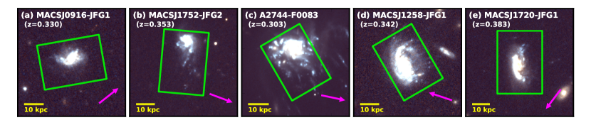
Figure 2: The zoom-in HST images of the five jellyfish galaxies with the size of $12^{\prime\prime}\times 12^{\prime\prime}$. Green boxes show the field-of-view of the GMOS/IFU 2-slit mode ($5^{\prime\prime}\times 7^{\prime\prime}$). Magenta arrows represent the directions to the cluster center (BCGs). The orientations are same as in Figure 1.

We selected five jellyfish galaxies in the MACS clusters (McPartland et al., 2016) and Abell 2744 (Owers et al., 2012) for our IFS observations: MACSJ0916-JFG1 ($z=0.330$), MACSJ1752-JFG2 ($z=0.353$), A2744-F0083 ($z=0.303$), MACSJ1258-JFG1 ($z=0.342$), and MACSJ1720-JFG1 ($z=0.383$). Among these five galaxies, A2744-F0083 and MACSJ1258-JFG1 host type I active galactic nuclei (AGN) in their center. We will describe this again with the Baldwin, Phillips & Terlevich (BPT) diagrams (Baldwin et al., 1981) in Section 4.1. The properties of the host clusters are summarized in Table 2.

Figure 1 shows the HST/ACS color composite images of the selected jellyfish galaxies and their host clusters. We display the locations of the brightest cluster galaxies (BCGs) and jellyfish galaxies in the host clusters. In this study, we set the marked BCGs as the center of each cluster. Figure 2 shows the zoom-in thumbnail images of the five jellyfish galaxies. We mark the FOV of the GMOS/IFU 2-slit mode (green boxes; $5\arcsec\times 7\arcsec$) and the direction to the cluster center (magenta arrows). In these HST optical images, all the jellyfish galaxies show disturbed and asymmetric morphology with blue tails and bright star-forming knots. MACSJ0916-JFG1 has a short ($\sim 5~{}{\rm kpc}$) tail at the eastern side of the galactic center and a few star-forming knots in the disk and tail. MACSJ1752-JFG2 shows not only an extended ($\sim 25~{}{\rm kpc}$) tail towards the southern direction, but also large bright knots with ongoing star formation around the disk. A2744-F0083 is the most spectacular object exhibiting large and bright star-forming knots and multiple stripped tails. MACSJ1258-JFG1 has a bright tail towards the northern direction with a length of $\sim 10~{}{\rm kpc}$ and small blue extraplanar knots outside the disk. MACSJ1720-JFG1 is the most distant galaxy in this study. This galaxy shows a star-forming tail in the northern region and a bright compressed region at its head. The FOV of the GMOS/IFU is wide enough to cover the substructures of the jellyfish galaxies except for a few faint tails at the western side of A2744-F0083.

For these jellyfish galaxies, there seems to be no clear trend between the direction of the tails and their direction towards the cluster center. Tails of MACSJ0916-JFG1 and MACSJ1752-JFG2 are extended in a direction nearly tangential to the cluster center. In contrast, tails of MACSJ1258-JFG1 and MACSJ1720-JFG1 are extended towards the opposite direction to the cluster center. Interestingly, A2744-F0083 has multiple tails extending towards the BCGs in the cluster center. This misalignment of the direction of tails and the direction to the cluster center has been also shown by the jellyfish galaxies in the GASP survey (Poggianti et al., 2016) and those in the IllustrisTNG simulation (Yun et al., 2019). This indicates that these jellyfish galaxies travel in various orbital trajectories within their host clusters, and do not necessarily travel in a radial direction.

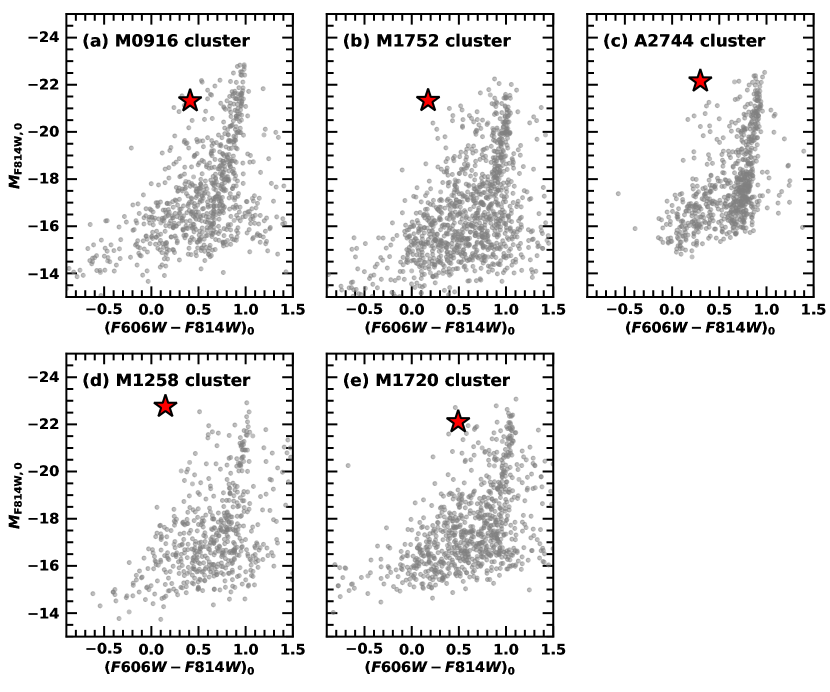
Figure 3: Color-magnitude diagrams of galaxies detected in the HST images of the host clusters. All colors and magnitudes are de-reddened by the foreground extinction magnitudes. Red star symbols show the data of the five jellyfish galaxies. Gray circles show the data of all extended sources with half-light radii larger than $0\farcs 2$ in the angular scale and $\gtrsim 1~{}{\rm kpc}$ in the physical scale.

Figure 3 shows the color-magnitude diagrams of galaxies in the HST fields of the host clusters. We ran SExtractor (Bertin & Arnouts, 1996) to detect sources in the HST images and measure their colors and magnitudes. For the color-magnitude diagrams, we plot the data of the extended sources (gray circles) with a half-light radius (FLUX_RADIUS) larger than 4 pixels ($0\farcs 2$ in the angular scale and $\gtrsim 1~{}{\rm kpc}$ in the physical scale). These diagrams clearly show the red sequence of cluster members in each HST field. The jellyfish galaxies in this study (red star symbols) have much bluer colors than the galaxies in the red sequence. This indicates that young stellar populations are more dominant in these jellyfish galaxies than in other cluster members.

Table 3: GMOS/IFU Observations of the Jellyfish Galaxies

Galaxy Name	MACSJ0916-JFG1	MACSJ1752-JFG2	A2744-F0083	MACSJ1258-JFG1	MACSJ1720-JFG1
Program ID	GS-2019A-Q-214	GN-2019A-Q-215	GS-2019B-Q-219	GN-2021A-Q-205	GN-2021A-Q-205
Instrument	GMOS-S	GMOS-N	GMOS-S	GMOS-N	GMOS-N
Observing mode	IFU two-slit	IFU two-slit	IFU two-slit	IFU two-slit	IFU two-slit
Grating & Filter	R150+GG455	R150+GG455	R400+CaT	R150+GG455	R150+GG455
$\lambda_{\rm obs}~{}({\rm\AA})$	$4550-9550$	$4690-9590$	$7820-9260$	$4690-9280$	$4700-9700$
$\lambda_{\rm rest}~{}({\rm\AA})$	$3420-7180$	$3470-7090$	$6000-7110$	$3490-6910$	$3430-7080$
Spectral resolution	1230	1260	2440	1200	1270
Total exposure (sec)	4320	15040	10320	9900	14400
Observing date (UT)	2019-03-04	2019-06-11	2019-08-09	2021-05-17	2021-06-21
Mean airmass	1.29	1.25	1.19	1.23	1.18
Standard star	GD108	Wolf1346	VMa2	Feige34	Feige34
Seeing FWHM	0.88″	0.50″	1.14″	0.71″	0.56″
Surface brightness limit	$4.9\times 10^{-20}$	$1.8\times 10^{-19}$	$2.7\times 10^{-19}$	$4.5\times 10^{-19}$	$2.1\times 10^{-20}$
(${\rm erg~{}s^{-1}~{}cm^{-2}~{}arcsec^{-2}}$)

2.2 Gemini GMOS/IFU Data

2.2.1 Observation

Table 3 summarizes our GMOS/IFU observation programs. The five jellyfish galaxies were observed in the 2019A/B and 2021A seasons (PI: Jeong Hwan Lee): MACSJ0916-JFG1, MACSJ1752-JFG2, A2744-F0083, MACSJ1258-JFG1, and MACSJ1720-JFG1. (PID: GN-2021A-Q-205). We obtained the IFU data of three galaxies (MACSJ1752-JFG2, MACSJ1258-JFG1, and MACSJ1720-JFG1) from the site of GMOS-North (GMOS-N) and two other targets (MACSJ0916-JFG1 and A2744-F0083) from GMOS-South (GMOS-S). All the observations used the GMOS/IFU 2-slit mode with an FOV of $5\arcsec\times 7\arcsec$.

We observed all galaxies with the exception of A2744-F0083 with the R150 grating and GG455 blocking filter, which securely covers a wide range of wavelengths from 4700Å to 9200Å in the observer frame ($\sim 3500-6900$Å in the rest frame). This coverage includes strong emission lines from [O II]$\lambda\lambda 3727,3729$ to [S II]$\lambda\lambda 6717,6731$. We derived the spectral resolution of the spectra from the telluric emission lines obtained by the sky fibers. The configuration of R150$+$GG455 has a low spectral resolution of $R\sim 1200$ at the wavelength of the ${\rm H\alpha}$ line. For A2744-F0083, the R400 grating and CaT filter were applied with the central wavelength of 8600Å. This combination had a limited wavelength coverage from 7820Å to 9260Å (6000-7110Å in the rest frame) but had better spectral resolution ($R\sim 2400$). As a result, the data of A2744-F0083 only covered emission lines from [O I]$\lambda 6300$ to [S II]$\lambda\lambda 6717,6731$.

MACSJ0916-JFG1 was observed at the GMOS-South with an exposure time of $4\times 1080~{}{\rm s}$ (total 1.2 hr) on the 2019-03-04 (UT). MACSJ1752-JFG2 was observed with the exposure time of $16\times 900~{}{\rm s}+640~{}{\rm s}$ (total 4.2 hr) during three nights starting from 2019-06-11 (UT). A2744-F0083 was observed with $12\times 860~{}{\rm s}$ (total 2.9 hr) on the UT dates from 2019-08-09 to 2019-08-30. In the 2021A season, MACSJ1258-JFG1 and MACSJ1720-JFG1 were observed with $11\times 900~{}{\rm s}$ (total 2.8 hr) and $16\times 900~{}{\rm s}$ (total 4.0 hr), respectively. The mean airmass of the data ranged from 1.2 to 1.3 for all targets. The median full widths at half maximum (FWHMs) of the seeing in our observations were measured from the acquisition images, ranging about $0\farcs 5-0\farcs 7$ at the GMOS-N and $0\farcs 9-1\farcs 2$ at the GMOS-S.

2.2.2 Data Reduction

We reduced the GMOS/IFU data using the GEMINI package in PyRAF. We used the tasks of GBIAS, GFREDUCE, and GFRESPONSE for bias subtraction and flat fielding with the Gemini Facility Calibration Unit (GCAL) flat. Since there were some missing fibers that the PyRAF/Gemini tasks could not find, we developed our own codes to correct the IFU mask definition file (MDF) for proper flat fielding. We performed the interactive tasks of GSWAVELENGTH to obtain the wavelength solution from the CuAr arcs. The scattered light interfering in the fiber gaps was removed by the 2-D surface model with the order of 3 in the GFSCATSUB task. After the preprocessing of the science frames, the cosmic rays and the sky lines were removed by GEMCRSPEC and GFSKYSUB tasks. Four standard stars were used for flux calibrations of our sample: GD108 (MACSJ0916-JFG1), Wolf1346 (MACSJ1752-JFG2), VMa2 (A2744-F0083), and Feige34 (MACSJ1258-JFG1 and MACSJ1720-JFG1). We carried out the flux calibrations by using GSCALIBRATE with the Chebyshev polynomials with an order of 11. These reduction processes created individual IFU data cubes with dispersions of $1.95{\rm~{}\AA~{}pixel^{-1}}$ for the R150 grating and $0.75{\rm~{}\AA~{}pixel^{-1}}$ for the R400. The spatial pixel scale of all cubes is $0\farcs 1~{}{\rm pixel^{-1}}$. We then carried out the spectral and spatial alignments of the cubes and combined them into one final cube for each target. We used these final data cubes for the analysis of the five jellyfish galaxies in this study.

Table 4: Optical and Near-infrared Archival Images of the Jellyfish Galaxies

Galaxy Name	Instrument	Filters	Survey
MACSJ0916-JFG1	HST/ACS	$F606W$, $F814W$	PID: 10491, 12166
	WISE	W1 (3.4 $\mu$m), W2 (4.6 $\mu$m)	All-Sky Data Release
MACSJ1752-JFG2	HST/ACS	$F435W$, $F606W$, $F814W$	PID: 12166, 12884, 13343
	Spitzer/IRAC	3.6 $\mu$m, 4.5 $\mu$m	PID: 12095
A2744-F0083	HST/ACS	$F435W$, $F606W$, $F814W$	PID: 13495, 15117
	Spitzer/IRAC	3.6 $\mu$m, 4.5 $\mu$m	PID: 83, 90257
MACSJ1258-JFG1	HST/ACS	$F606W$, $F814W$	PID: 10491, 12166
	Spitzer/IRAC	3.6 $\mu$m, 4.5 $\mu$m	PID: 12095
MACSJ1720-JFG1	HST/ACS	$F435W$, $F606W$, $F814W$	PID: 12455
	Spitzer/IRAC	3.6 $\mu$m, 4.5 $\mu$m	PID: 545, 90213, 90233

2.3 Archival Images

We used optical and near-infrared (NIR) images of our targets to estimate their stellar mass. This is because the signal-to-noise ratios (S/N) of the GMOS/IFU spectra were not high enough to derive their stellar mass from spectral continuum fitting. We collected the images from archives of the HST for optical views and Wide-field Infrared Survey Explorer (WISE) and Spitzer for NIR views. With these multi-wavelength images, we compared the morphology of the stellar emission with that of the gas emission observed by the GMOS/IFU spectral maps. In addition, we derived stellar masses of the jellyfish galaxies using these images. Table 4 lists the information of the archival images we used for analysis.

2.3.1 HST Optical Images

We retrieved the HST/ACS images of the five jellyfish galaxies from the Mikulski Archive for Space Telescopes (MAST). We obtained the individual calibrated images (*_flc.fits or *_flc.fits) and drizzled them by using the TweakReg and AstroDrizzle tasks in DrizzlePac. We combined all the images with a pixel scale of $0\farcs 05~{}{\rm pixel^{-1}}$.

MACSJ0916-JFG1 and MACSJ1258-JFG1 were covered with two optical bands of ACS/$F606W$ and ACS/$F814W$. Both bands were observed during the HST program of the snapshot survey of the massive galaxy clusters (PI: H. Ebeling). The drizzled HST images had exposure times of 1200 sec for $F606W$ and 1440 sec for $F814W$.

For MACSJ1752-JFG2, we utilized three ACS optical bands ($F435W$, $F606W$, and $F814W$). These images were obtained through a snapshot survey (PI: H. Ebeling) and a program for weak lensing analysis (PI: D. Wittmann). The exposure times of the final images were 2526 sec ($F435W$), 3734 sec ($F606W$), and 6273 sec ($F814W$).

A2744-F0083 was covered in the HFF (Lotz et al., 2017) and the Buffalo HST survey (Steinhardt et al., 2020). We utilized three ACS optical bands ($F435W$, $F606W$, and $F814W$) from the surveys. These drizzled images had the longest exposure times among our targets: 45747 sec ($F435W$), 26258 sec ($F606W$), and 108984 sec ($F814W$).

MACSJ1720-JFG1 was observed by a multi-wavelength observation program for the lensing analysis of massive clusters (PI: M. Postman). We utilized three ACS optical bands ($F435W$, $F606W$, and $F814W$). The images had exposure times of 2040 sec ($F435W$), 2020 sec ($F606W$), and 3988 sec ($F814W$), respectively.

2.3.2 Spitzer and WISE NIR Images

We obtained archival NIR images taken with Spitzer/IRAC from the Spitzer Heritage Archive (SHA) for all galaxies with the exception of MACSJ0916-JFG1, which was not observed by Spitzer. For MACSJ0916-JFG1, we retrieved the WISE images from the NASA/IPAC Infrared Science Archive (IRSA). The images were taken from the WISE All-Sky Data Release and had exposure times of 7.7 sec for W1 ($3.4~{}{\rm\mu m}$) and W2 ($4.6~{}{\rm\mu m}$) bands. As the sensitivity of the W3 ($12~{}{\rm\mu m}$) and W4 ($22~{}{\rm\mu m}$) bands are too low, we only used the W1 and W2 images for our analysis. MACSJ1752-JFG2 and MACSJ1258-JFG1 were observed through an IRAC snapshot imaging survey of massive clusters (PID: 12095, PI: Egami) with exposure times of 94 sec ($3.6~{}{\rm\mu m}$) and 97 sec ($4.5~{}{\rm\mu m}$). As for A2744-F0083, we combined a total of 20 IRAC exposures from two science programs: PID 83 (2 exposures; PI: Rieke) and PID 90257 (18 exposures; PI: Soifer). The exposure times of the combined images were 1878 sec ($3.6~{}{\rm\mu m}$) and 1936 sec ($4.5~{}{\rm\mu m}$). MACSJ1720-JFG1 had 6 IRAC exposures from three programs: PID 545 (2 exposures), PID 90213 (3 exposures), and PID 90233 (1 exposure). After combining these images, we obtained the final images with exposure times of 374 sec ($3.6~{}{\rm\mu m}$) and 387 sec ($4.5~{}{\rm\mu m}$).

3 Analysis

3.1 Emission Line Fitting

In this study, we focused on analyzing strong emission lines such as ${\rm H\alpha}$, ${\rm H\beta}$, [O III], [N II], and [S II] given the low S/N of the spectral continuum in the GMOS/IFU data. First, we removed the background spectral noise from the combined IFU cubes. We took the median value of the spaxels at the edge of the cubes, which has no object signal, as background noise in each cube. We subtracted these noise patterns from all the pixels in the IFU cubes. This process cleaned the unnecessary instrumental noise pattern of the spectra. Next, we carried out Voronoi binning with the Python vorbin package (Cappellari & Copin, 2003) to obtain high S/N for emission line analysis in each bin. The S/N in the Voronoi bins ranged from 30 to 60 at the ${\rm H\alpha}$+[N II] regions for the jellyfish galaxies, depending on the exposure time and the quality of the data. The numbers of the final Voronoi bins in the IFU cubes were 42 (MACSJ0916-JFG1), 147 (MACSJ1752-JFG2), 175 (A2744-F0083), 215 (MACSJ1258-JFG1), and 166 (MACSJ1720-JFG1). Then, we subtracted the continuum from the spectra of all the Voronoi bins. We performed the Gaussian smoothing for continuum subtraction because it was difficult to carry out the spectral continuum fitting (e.g., pPXF) for the Voronoi bins with low S/N in the outer region. For the Gaussian smoothing of the continuum, we applied a kernel width of 10Å after masking the emission lines.

We then fitted strong emission lines (${\rm H\beta}$, [O III]$\lambda\lambda 4959,5007$, ${\rm H\alpha}$, [N II]$\lambda\lambda 6548,6584$, and [S II]$\lambda\lambda 6717,6731$) with the Markov chain Monte Carlo (MCMC) method using the Python emcee package (Foreman-Mackey et al., 2013). For A2744-F0083, we fitted only the ${\rm H\alpha}$+[N II] doublet and [S II] doublet lines. We applied multiple Gaussian functions for fitting the line profiles. For the narrow components of the emission lines, we used three Gaussian profiles for the ${\rm H\beta}$+[O III] and ${\rm H\alpha}$+[N II] regions and two for the [S II] doublet. In the case of AGN host galaxies (A2744-F0083 and MACSJ1258-JFG1), more profiles were added for fitting the broad components of the ${\rm H\beta}$+[O III] and ${\rm H\alpha}$+[N II] regions.

We initially fitted the emission lines from the central Voronoi bins with high S/N. We then used the initial solutions to run the MCMC process for all the bins. We defined the prior distributions of parameters as Gaussian functions centered on the initial solutions. We implemented the MCMC process in emcee with 50 walkers and 2000 steps. After finishing all the MCMC steps of walkers, we measured the skewness and kurtosis of the posterior distributions of parameters to check the reliability of our parameter estimation. We rejected solutions from Voronoi bins with values of skewness and kurtosis higher than 0.5 or lower than $-0.5$. We took the median values of the posterior distributions as the burn-in solutions of the MCMC process.

In Figure 4, we plot the GMOS/IFU spectra in the central regions (within a radius of $0\farcs$4) of our targets. We used these integrated spectra for obtaining the initial solutions of the line fitting in all the Voronoi bins. We plot the original spectra and the continuum subtracted spectra in the left and middle panels, respectively. The right panels show the zoom-in spectra at the ${\rm H\alpha}$+[N II] regions overlaid with the best-fit models (pink solid lines). For the AGN host galaxies, we added two more profiles (red dashed lines) for broad components of this region. Residuals (green solid lines) show that the best-fit models represent the spectra well.

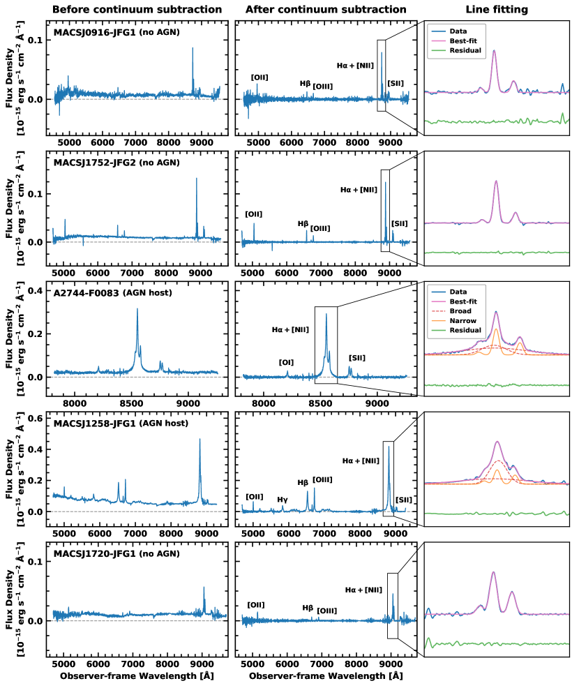
Figure 4: The integrated spectra within a radius of within a radius of $0\farcs 4$ from the galactic center of jellyfish galaxies in this study. The left panels show the original spectra before continuum subtraction, and the middle panels show the continuum subtracted spectra. In the middle panels, several strong emission lines are marked in each spectrum. The right zoom-in panels show the ${\rm H\alpha}$+[N II] region of each galaxy. We plot the observed spectra (blue solid lines), our best-fit models (pink solid lines), and residuals (green solid lines). In the case of AGN host galaxies, we plot narrow and broad components of the emission lines with orange solid lines and red dashed lines, respectively.

3.2 Measurements of SFRs, Gas Velocity Dispersion, and Stellar Masses

3.2.1 $H\alpha$-derived SFRs

In this section, we describe how we estimated the SFRs based on the emission line analysis. We derived the SFRs of jellyfish galaxies from their ${\rm H\alpha}$ luminosity that was corrected for stellar absorption, extinction, and AGN contamination.

Stellar absorption affects the observed fluxes of the Balmer lines such as ${\rm H\alpha}$ and ${\rm H\beta}$. Since the S/N of stellar continuum in our GMOS/IFU data is too low to do the full spectrum fitting, we took a simple approach for absorption correction by assuming constant equivalent widths (EWs) of the Balmer absorption lines (Hopkins et al., 2003; Gunawardhana et al., 2011). We used the following formula for the absorption correction,

$$S_{\rm H\alpha}=F_{\rm H\alpha}\times\frac{{\rm EW_{H\alpha}}+{\rm EW}_{c}}{\rm EW_{H\alpha}},$$ (1)

where $S_{\rm H\alpha}$ is the absorption-corrected ${\rm H\alpha}$ flux, $F_{\rm H\alpha}$ is the observed ${\rm H\alpha}$ flux, ${\rm EW_{H\alpha}}$ is the observed ${\rm H\alpha}$ EW, and ${\rm EW}_{c}$ is the EW for stellar absorption. Hopkins et al. (2003) suggested that the median intrinsic value of ${\rm EW}_{c}$ is 2.6Å for the SDSS sample of star-forming galaxies but this value would be reduced to 1.3Å in the real SDSS spectra. This is because SDSS spectra have sufficient spectral resolution ($R\sim 2000$) to resolve broad stellar absorption profiles (see Figure 7 in Hopkins et al. (2003)). Therefore, we adopted ${\rm EW}_{c}=1.3{\rm\AA}$ for A2744-F0083 observed by the R400 grating with a similar resolution ($R\sim 2400$) to the SDSS and ${\rm EW}_{c}=2.6{\rm\AA}$ for the remaining targets observed with the R150 grating ($R\sim 1200$). We applied the same EWs to correct the absorption of ${\rm H\beta}$ line.

We subsequently corrected for internal dust extinction and foreground extinction. For the dust extinction correction, we used the absorption-corrected flux ratio of the ${\rm H\alpha}$ and ${\rm H\beta}$ lines, otherwise known as the Balmer decrement. We assumed an intrinsic ${\rm H\alpha}$ to ${\rm H\beta}$ flux ratio of 2.86 for the case B recombination with $T_{e}=10000~{}{\rm K}$ and adopted the Cardelli et al. (1989) extinction law. The equations for extinction correction are given as below,

$$A_{\rm H\alpha}=k_{\rm H\alpha}\times E(B-V),$$ (2)

where $A_{\rm H\alpha}$ is the extinction magnitude of the ${\rm H\alpha}$ flux, $k_{\rm H\alpha}$ is the extinction coefficient for ${\rm H\alpha}$, and $E(B-V)$ is the color excess. We adopted $k_{\rm H\alpha}=2.53$ from Cardelli et al. (1989). The color excess can be derived from the equation (3).

$$E(B-V)=2.33\times\log\left[\frac{S_{\rm H\alpha}/S_{\rm H\beta}}{2.86}\right],$$ (3)

where $S_{\rm H\alpha}/S_{\rm H\beta}$ is the absorption-corrected ${\rm H\alpha}$ to ${\rm H\beta}$ flux ratio. We also corrected for foreground extinction using the reddening magnitudes from Schlafly & Finkbeiner (2011) (see Table 2).

From the corrected ${\rm H\alpha}$ flux, we derived the SFRs using the following relation given by Kennicutt (1998) assuming the Chabrier (2003) initial mass function (IMF),

$${\rm SFR_{H\alpha}}=4.6\times 10^{-42}L_{\rm H\alpha},$$ (4)

where ${\rm SFR_{H\alpha}}$ is the ${\rm H\alpha}$-based SFR with unit of $M_{\odot}~{}{\rm yr^{-1}}$ and $L_{\rm H\alpha}$ is the ${\rm H\alpha}$ luminosity corrected for stellar absorption and extinction. The extinction law and IMF adopted in this paper are consistent with those in the GASP studies.

Throughout these processes, we rejected the Voronoi bins with S/N (${\rm H\alpha}$) lower than 3. In addition, we excluded the Voronoi bins classified as AGN and low-ionization nuclear emission-line regions (LINERs) in the BPT diagram, as shown in Figures 5 and 6 (see Section 4.1). For the Voronoi bins with $\rm S/N<3$ in ${\rm H\beta}$ and [O III], we used the [N II]$\lambda 6584/{\rm H\alpha}$ ratio for the classification instead. We classified the Voronoi bins with log([N II]$\lambda 6584/{\rm H\alpha})>-0.4$ as AGN and excluded them from consideration. We also included the Voronoi bins with ${\rm S/N~{}(H\alpha)>3}$ but weak S/N ($<3$) of ${\rm H\beta}$ and the BPT forbidden lines ([O III] and [N II]) for computing the SFR, as done in Medling et al. (2018).

As a result, total SFR values in each correction step (continuum subtraction, absorption correction, and extinction correction) for the five jellyfish galaxies are listed in Table 5. This table shows that dust extinction correction takes much more effect on the SFR values than the two other correction steps.

Table 5: Total SFR Calculations of the Jellyfish Galaxies in Each Step

Galaxy Name	Initial SFR	Continuum subtraction	Absorption correction	Extinction correction
	($M_{\odot}~{}{\rm yr^{-1}}$)	($M_{\odot}~{}{\rm yr^{-1}}$)	($M_{\odot}~{}{\rm yr^{-1}}$)	($M_{\odot}~{}{\rm yr^{-1}}$)
(1)	(2)	(3)	(4)	(5)
MACSJ0916-JFG1	7.21	5.47	5.64	7.12
MACSJ1752-JFG2	11.43	8.79	9.03	30.43
A2744-F0083∗	12.76	9.08	9.17	22.00
MACSJ1258-JFG1∗	17.89	10.37	11.37	35.71
MACSJ1720-JFG1	13.75	7.14	7.62	17.37

3.2.2 Gas Velocity Dispersion

We derived the gas velocity dispersion ($\sigma_{v,{\rm gas}}$) using the standard deviation of ${\rm H\alpha}$ emission line corrected for beam-smearing and instrumental dispersion. Beam-smearing occurs when the observed line in a IFU spaxel is blended with the lines from the neighboring spaxels, which makes a broader line profile. Since the seeing FWHM in our observations ranged from $0\farcs 5$ to $1\farcs 1$, which corresponds from 5 to 11 spaxels for the GMOS/IFU, this effect significantly contributes to the velocity dispersion. To correct for beam-smearing, we followed the method described in Appendix A in Stott et al. (2016). Using the artificial VLT/KMOS data cube with similar seeing and pixel scale to our GMOS/IFU data, they suggested that a linear subtraction of velocity gradient ($\Delta v/\Delta r$) from the observed velocity dispersion can effectively correct for beam-smearing. This method is described with the equation below,

$$\sigma_{v,{\rm cor}}=\sigma_{v,{\rm obs}}-\frac{\Delta v}{\Delta r},$$ (5)

where $\sigma_{v,{\rm cor}}$ is the beam-smearing corrected velocity dispersion, $\sigma_{v,{\rm obs}}$ is the observed velocity dispersion, and $\Delta v/\Delta r$ is the maximum velocity gradient at a distance equivalent to the seeing FWHM from the center of a galaxy. Our data cubes showed maximum velocity gradients of $\Delta v/\Delta r=4.9~{}{\rm km~{}s^{-1}~{}spaxel^{-1}}$ (MACSJ0916-JFG1), $8.2~{}{\rm km~{}s^{-1}~{}spaxel^{-1}}$ (MACSJ1752-JFG2), $10.6~{}{\rm km~{}s^{-1}~{}spaxel^{-1}}$ (A2744-F0083), $10.5~{}{\rm km~{}s^{-1}~{}spaxel^{-1}}$ (MACSJ1258-JFG1), and $14.8~{}{\rm km~{}s^{-1}~{}spaxel^{-1}}$ (MACSJ1720-JFG1). For comparison, Stott et al. (2016) measured $\Delta v/\Delta r=13.4~{}{\rm km~{}s^{-1}~{}spaxel^{-1}}$.

Then, we subtracted the GMOS/IFU instrumental dispersion from the beam-smearing corrected dispersion. The instrumental velocity dispersion was derived from a single Gaussian fitting of the sky emission lines which were extracted during the data reduction process. We obtained the instrumental velocity dispersion at the wavelength of ${\rm H\alpha}$ for our GMOS/IFU data: $\sigma_{v,{\rm inst}}=103.1~{}{\rm km~{}s^{-1}}$ (MACSJ0916-JFG1), $101.4~{}{\rm km~{}s^{-1}}$ (MACSJ1752-JFG2), $52.2~{}{\rm km~{}s^{-1}}$ (A2744-F0083), $106.1~{}{\rm km~{}s^{-1}}$ (MACSJ1258-JFG1), and $100.1~{}{\rm km~{}s^{-1}}$ (MACSJ1720-JFG1). We used a quadrature removal of instrumental dispersion,

$$\sigma_{v,{\rm gas}}^{2}=\sigma_{v,{\rm cor}}^{2}-\sigma_{v,{\rm inst}}^{2},$$ (6)

where $\sigma_{v,{\rm gas}}$ is the corrected gas velocity dispersion and $\sigma_{v,{\rm inst}}$ is the instrumental velocity dispersion.

3.2.3 Stellar Masses

We estimated the stellar masses ($M_{\ast}$) of our jellyfish galaxies using the NIR images described in Section 2.3. The GASP studies derived the stellar masses from the spectral continuum fitting (Poggianti et al., 2017). However, our GMOS/IFU data showed too low S/N of the continuum to apply the same method as the GASP studies. Instead, we converted the NIR fluxes of the Spitzer/IRAC $3.6~{}{\rm\mu m}$ and $4.5~{}{\rm\mu m}$ (W1 and W2 in the case of WISE data) to stellar masses following the relation from Eskew et al. (2012).

$$M_{\ast}=\xi\times 10^{5.65}\times S^{2.85}_{\rm 3.6\mu m}S^{-1.85}_{\rm 4.5\mu m}\times(d_{L}/0.05)^{2}~{}M_{\odot},$$ (7)

where $\xi$ is the conversion factor from the Salpeter IMF (Salpeter, 1955) to other IMFs, $S_{\rm 3.6\mu m}$ and $S_{\rm 4.5\mu m}$ are the NIR fluxes of $3.6~{}{\rm\mu m}$ and $4.5~{}{\rm\mu m}$ in Jy, and $d_{L}$ is the luminosity distance in Mpc. We applied $\xi=0.54$ for the Chabrier IMF (Chabrier, 2003) with a mass range from 0.1 to 100 $M_{\odot}$. This method has been used for estimating the stellar masses of star-forming galaxies in Abell 2744 (Rawle et al., 2014).

We utilized photutils v1.0.2 (Bradley et al., 2021) to measure the NIR fluxes of the jellyfish galaxies. We performed aperture photometry using rectangular apertures with the size of the GMOS/IFU FOV ($5^{\prime\prime}\times 7^{\prime\prime}$) for all targets except for MACSJ0916-JFG1. Since MACSJ0916-JFG1 was only observed by WISE with poor spatial resolution ($\rm FWHM\sim 6\farcs 4$ in W1 and W2; Wright et al., 2010), we increased the aperture size to twice the FWHM of the WISE images. The derived stellar masses are listed in Table 6, ranging from ${\rm log}~{}M_{\ast}/M_{\odot}=9.84$ to 10.90.

3.3 Definition of Disk and Tail

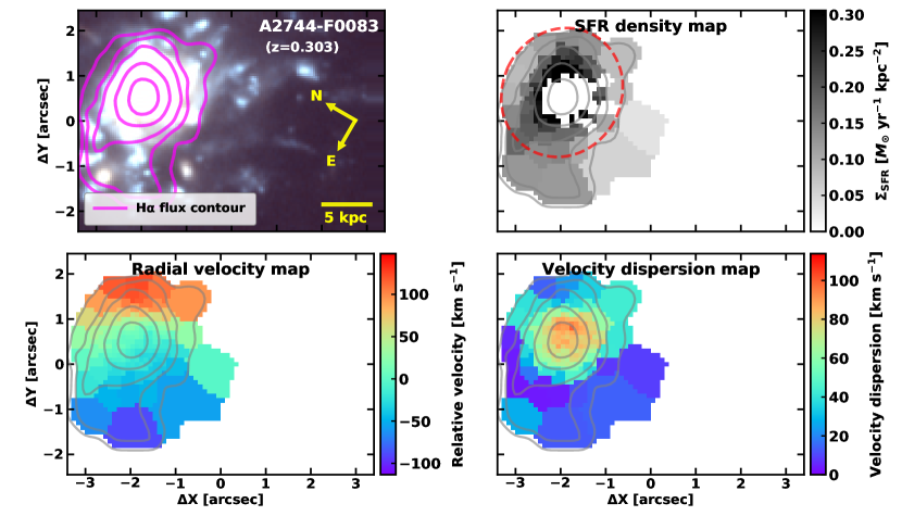
Figure 9: Same figure as Figure 7 but for A2744-F0083.

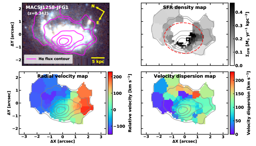
Figure 10: Same as Figure 7 but for MACSJ1258-JFG1.

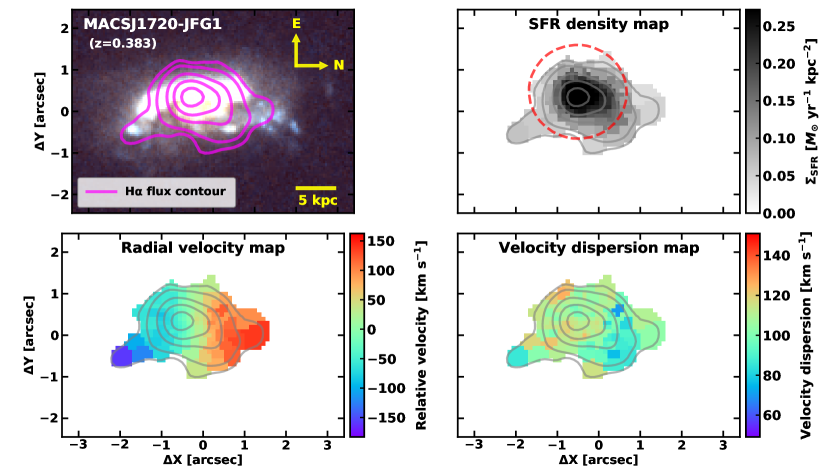
Figure 11: Same as Figure 7 but for MACSJ1720-JFG1.

In this study, we spatially divided a jellyfish galaxy into two components – “disk” and “tail”. The disk corresponds to the main body of the galaxy, and the tail is the extraplanar region composed of ram-pressure stripped ISM outside the disk. To compare our results with the GASP studies, we used the definition of the galaxy boundary between the disk and tail as described in Poggianti et al. (2019) and Gullieuszik et al. (2020). We made use of the emission line maps of the ${\rm H\alpha}$+[N II] region from the GMOS/IFU data. Although the GASP studies used continuum maps of the ${\rm H\alpha}$+[N II] region, it was difficult for this study to use continuum maps due to low S/N. The background level and standard deviation ($1\sigma$) were estimated using the DAOPHOT MMM algorithm on the $3\sigma$-clipped data in the emission line maps. We then manually masked the disturbed region of the galaxy, removing tails and extraplanar clumps. With the masked map, we carried out elliptical isophote fitting using PyRAF/Ellipse. The galaxy boundary between the disk and tail was defined as an elliptical isophote with a surface brightness of $1\sigma$ above the background level. The upper right panels of Figures 7-11 display the defined boundaries in the five jellyfish galaxies with red dashed ellipses.

Although we followed the definition from the GASP studies, the boundary between the disk and tail used in this paper could not be fully consistent with that in the GASP studies. This is because manual masking of disturbed regions is a little arbitrary and the spatial resolution of the GMOS/IFU data is quite different from that of MUSE data in the physical scale (e.g., the mean seeing FWHM $0\farcs 7$ corresponds to $>3~{}{\rm kpc}$ for our targets but $\sim 0.7~{}{\rm kpc}$ in the GASP targets). These limitations could contribute to large fluctuations of the fraction of SFR in tails as shown in Table 6.

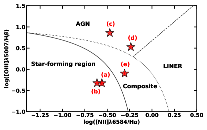
Figure 5: A BPT diagram of the integrated spectra of the five jellyfish galaxies. Each galaxy is marked with the same order as in Figure 2: (a) MACSJ0916-JFG1, (b) MACSJ1752-JFG2, (c) A2744-F0083, (d) MACSJ1258-JFG1, and (e) MACSJ1720-JFG1. We plot a solid line from Kauffmann et al. (2003), a dotted line from Kewley et al. (2001), and a dashed line from Sharp & Bland-Hawthorn (2010) to divide star-forming, composite, AGN, and LINER regions in this diagram.

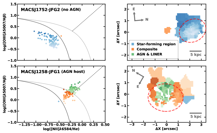
Figure 6: Left panels: BPT diagrams of the Voronoi bins with ${\rm S/N}>3$ in MACSJ1752-JFG2 (upper: a non-AGN host galaxy) and MACSJ1258-JFG1 (lower: an AGN host galaxy). The colors of the circle symbols represent the BPT classifications: star-forming (blue), composite (orange), and AGN$+$LINER regions (green). We color-code each symbol with the value of log ([O III] $\lambda 5007/{\rm H}\beta)$. Right panels: Spatial maps of the regions classified in the BPT diagrams. Here we exclude the Voronoi bins with S/N lower than 3. Red dashed ellipse represents the boundary of the disk and tail of this galaxy. The orientation and distance scale are marked in the figure.

4 Ionized Gas Properties of the Jellyfish Galaxies

4.1 BPT Diagnostics

In Figure 5, we display the BPT diagram ([O III]$\lambda$5007/${\rm H\beta}$ vs. [N II]$\lambda$6584/${\rm H\alpha}$) of the five jellyfish galaxies using the narrow components of the emission lines from their integrated spectra. All data used except for A2744-F0083 were taken with the GMOS/IFU. For the BPT diagram of A2744-F0083, we derived their flux ratios from the AAOmega spectra (Owers et al., 2012) because the GMOS/IFU spectra of this galaxy did not cover the ${\rm H\beta}$ and [O III] region. To determine the gas ionization mechanisms of each galaxy, we classify galaxies into four regions (star-forming, composite, AGN, and LINER) by adopting the well-known boundaries from Kewley et al. (2001), Kauffmann et al. (2003), and Sharp & Bland-Hawthorn (2010), as done in the GASP studies.

MACSJ0916-JFG1 (a) and MACSJ1752-JFG1 (b) are located in the star-forming region, showing the lowest flux ratios of log([O III]$\lambda 5007/{\rm H\beta})<-0.3$ and log([N II]$\lambda 6584/{\rm H\alpha})<-0.6$ among our sample. A2744-F0083 (c) and MACSJ1258-JFG1 (d) are genuine AGN host galaxies with log([O III]$\lambda 5007/{\rm H\beta})>0.5$. These galaxies also show broad components of the Balmer emission lines (${\rm H\alpha}$ and ${\rm H\beta}$) in their spectra, indicating that they are type I AGNs. MACSJ1720-JFG1 (e) is located in the composite region, showing a higher ratio of log([N II]$\lambda 6584/{\rm H\alpha})\sim-0.3$ than those from the two star-forming galaxies (log([N II]$\lambda 6584/{\rm H\alpha})\sim-0.6$). This indicates that the gas ionization in MACSJ1720-JFG1 cannot be solely explained by star formation. However, it is difficult to say that this galaxy hosts a type I AGN in its center, considering that its Balmer emission lines did not show any broad components in our GMOS/IFU spectra and were fitted well with single Gaussian components. It seems that other excitation mechanisms such as shocks (Rich et al., 2011) or heat conduction (Boselli et al., 2016) could be responsible for ionizing photons in this galaxy.

Figure 6 shows the BPT diagrams of Voronoi bins (left) and their spatial maps (right) of the two jellyfish galaxies, which have relatively high S/N of the BPT emission lines, as examples of a non-AGN host galaxy (MACSJ1752-JFG2) and an AGN host galaxy (MACSJ1258-JFG1). We only plot the bins with S/N higher than 3 for all the BPT emission lines. In the spatial map, we display all bins with BPT classifications of star-forming (blue), composite (orange), and AGN+LINER (green). For the remaining three galaxies, the Voronoi bins of the GMOS/IFU data show very low S/N of ${\rm H\beta}$ and [O III] lines (MACSJ0916-JFG1 and MACSJ1720-JFG1) or do not cover the wavelength range of the ${\rm H\beta}$ and [O III] lines (A2744-F0083). We also plot the boundary between the disk and tail of each galaxy (red dashed ellipse) as obtained from the method described in Section 3.3.

For MACSJ1752-JFG2, almost all bins belong to the star-forming region except for one bin in the tail region. The central region shows log([N II]$\lambda 6584/{\rm H\alpha})\sim-0.6$ and log([O III]$\lambda 5007/{\rm H\beta})\sim-0.3$, which are consistent with typical star-forming galaxies. It is also remarkable that the eastern tail region exhibits a higher [O III]/${\rm H\beta}$ ratio (log([O III]$\lambda 5007/{\rm H\beta})>0$) and a lower [N II]/${\rm H\alpha}$ ratio (log([N II]$\lambda 6584/{\rm H\alpha})<-0.75$) than the central region. The “composite” bin in the southern tail has marginally low S/N, such that the gas ionization source is not clear.

MACSJ1258-JFG1 has high flux ratios of log([O III]$\lambda 5007/{\rm H\beta})\sim 0.5$ and log([N II]$\lambda 6584/{\rm H\alpha})\sim-0.25$, indicating that it hosts an AGN. In this figure, several Voronoi bins in the central region and the head region in the east show low S/N of ${\rm H\beta}$ and [O III] lines. However, the Voronoi bins with ${\rm S/N}>3$ show that there is a clear radial gradient of the BPT line ratios from the center to the outer region. The outer disk and tail regions on the western side are classified as composite regions, implying that both star formation and shock-heating mechanisms contribute to gas ionization there.

4.2 SFRs, Gas Kinematics, and Dynamical States

We mainly analyze the ionized gas properties of each jellyfish galaxy using ${\rm H\alpha}$ emission lines. From Figures 7 to 11, we map the distributions of the ${\rm H\alpha}$ flux, the SFR surface density ($\Sigma_{\rm SFR}$), the radial velocity, and the gas velocity dispersion. We select the Voronoi bins with ${\rm S/N~{}(H\alpha)}>3$ for the analysis. Table 6 lists the stellar masses, dust extinction, SFRs, tail SFR fraction of total SFR ($f_{\rm SFR}={\rm SFR(tail)/SFR(total)}$), and gas kinematics of the jellyfish galaxies.

To compute and correct the SFRs, we derive dust extinction magnitudes from the flux-weighted mean Balmer decrement (${\rm H\alpha/H\beta}$). While the Balmer decrement and the extinction magnitude can slightly decrease from the center to the outskirts (a median decrease of $\sim 0.25~{}{\rm mag}$ reported in Poggianti et al. (2017)), we choose to assume a constant value throughout the galaxy due to the poor S/N of the ${\rm H\beta}$ emission lines in the outer regions. As a result, the five jellyfish galaxies in this study shows a median total SFR of 22.0 $M_{\odot}~{}{\rm yr^{-1}}$ and a median tail SFR of 6.8 $M_{\odot}~{}{\rm yr^{-1}}$. These SFRs are much higher than those of the GASP sample, with a median total SFR of 1.1 $M_{\odot}~{}{\rm yr^{-1}}$ and a median tail SFR of 0.03 $M_{\odot}~{}{\rm yr^{-1}}$. In addition, the median SFR fraction in the tail is also much higher in this study ($f_{\rm SFR}=22\%$) than in the GASP studies ($f_{\rm SFR}=3\%$). Lee et al. (2022) presented a detailed comparison of the star formation activity of the five jellyfish galaxies in this study with that of other known jellyfish galaxies including the GASP sample, considering galaxy stellar mass, redshift, and jellyfish morphology. As a result, they suggested a positive correlation between the star formation activity of jellyfish galaxies and the host cluster properties.

For ionized gas kinematics, we derive radial velocities using the peak wavelength measured from fitting. We show line-of-sight radial velocity maps measured with respect to the central Voronoi bins. Following the definition used in Wisnioski et al. (2015), We calculate the maximum rotational velocity at a circularized radius of the disk ($R_{\rm disk,c}=\sqrt{ab}$, where $a$ and $b$ are the galactocentric radii of the semi-major and semi-minor axis) as an indicator of the rotational speed of ionized gas within the disk.

In addition, we derive gas velocity dispersions as described in Section 3.2.2 to investigate the dynamical states of the ionized gas in each jellyfish galaxy. The median ${\rm H\alpha}$ velocity dispersion obtained by the GASP studies is $27~{}{\rm km~{}s^{-1}}$, suggesting that the ${\rm H\alpha}$-emitting clumps are dynamically cold (Bellhouse et al., 2019; Poggianti et al., 2019). With this information, we compare the distribution of the gas velocity dispersions in our sample with that of the GASP jellyfish galaxies.

Table 6: Properties of the Jellyfish Galaxies

Galaxy Name	$\log M_{\ast}$	${\rm H\alpha/H\beta}$	$A_{V}$	Total SFR	Tail SFR	$f_{\rm SFR}$	$|\Delta v|_{\rm disk}$	$\sigma_{v,{\rm gas}}$
	($M_{\odot}$)		(mag)	($M_{\odot}~{}{\rm yr^{-1}}$)	($M_{\odot}~{}{\rm yr^{-1}}$)	(%)	(${\rm km~{}s^{-1}}$)	(${\rm km~{}s^{-1}}$)
(1)	(2)	(3)	(4)	(5)	(6)	(7)	(8)	(9)
MACSJ0916-JFG1	10.18	$3.16\pm 0.29$	0.31	$7.12\pm 0.36$	$0.56\pm 0.26$	7.9	54.4	$30.0\pm 13.0$
MACSJ1752-JFG2	9.84	$4.78\pm 0.10$	1.61	$30.43\pm 0.17$	$6.76\pm 0.13$	22.2	73.2	$43.1\pm 12.6$
A2744-F0083∗	10.59	$4.14\pm 0.06$	1.16	$22.00\pm 0.10$	$7.53\pm 0.08$	34.2	89.5	$45.3\pm 5.3$
MACSJ1258-JFG1∗	10.90	$4.64\pm 0.19$	1.52	$35.71\pm 0.25$	$16.80\pm 0.20$	47.0	134.5	$100.5\pm 15.0$
MACSJ1720-JFG1	10.64	$4.05\pm 1.40$	1.09	$17.37\pm 1.12$	$3.28\pm 0.81$	18.9	103.5	$104.5\pm 15.8$

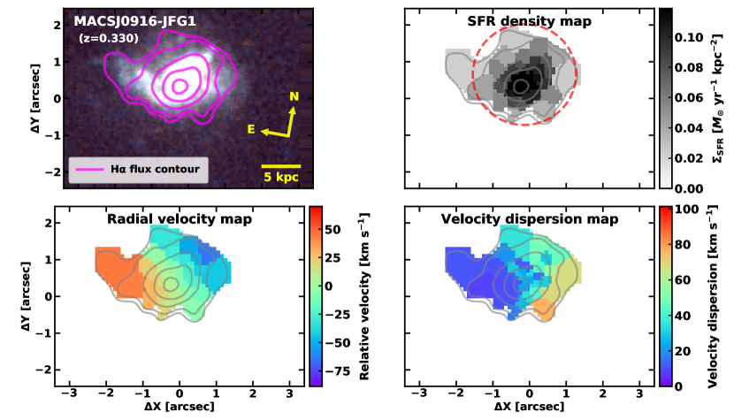
Figure 7: Upper left: HST color image of MACSJ0916-JFG1 overlaid with the ${\rm H\alpha}$ flux contour (magenta solid lines) derived from the GMOS/IFU data. We mark the orientation, distance scale, and redshift of this galaxy. Upper right: The SFR density (${\rm\Sigma_{SFR}}$) map estimated from the ${\rm H\alpha}$ luminosity. Red dashed circle represents the boundary of the disk and tail of this galaxy. Gray contours denote the spatial distribution of ${\rm H\alpha}$ flux. Right color bar shows the scale and range of the values. Lower left: The radial velocity map derived from the peak wavelength of ${\rm H\alpha}$ emission line. We display the relative velocity of each bin with respect to the central Voronoi bin with the highest ${\rm H\alpha}$ flux. Lower right: The gas velocity dispersion map derived from the width of ${\rm H\alpha}$ emission line.

4.2.1 MACSJ0916-JFG1

In Figure 7, it is clear that the ${\rm H\alpha}$ flux distribution of MACSJ0916-JFG1 is well-matched with its optical light distribution. The asymmetric feature of the ${\rm H\alpha}$ flux perfectly reproduces the eastern tail in the optical image. The ${\rm H\alpha}$ flux contours confirm that recent star formation has occurred in the blue knots in the disk and tail.

In the SFR surface density map, we distinguish the disk and tail regions as described in Section 3.3. The disk region within the $1\sigma$ boundary (red dashed ellipse) includes most of the Voronoi bins except for those in the eastern tail. The SFR surface density is highly concentrated in the central region. The flux-weighted mean of the Balmer decrement is 3.16, corresponding to a $V$-band extinction magnitude of 0.31 mag, which is the lowest value among our sample. The total SFR is estimated to be 7.12 $M_{\odot}~{}{\rm yr^{-1}}$, with 6.55 $M_{\odot}~{}{\rm yr^{-1}}$ for the disk and 0.56 $M_{\odot}~{}{\rm yr^{-1}}$ for the tail. The tail SFR fraction of total SFR is $f_{\rm SFR}=7.9\%$, which is the lowest value out of the five jellyfish galaxies.

This galaxy shows a weak rotation of ionized gas in its disk. The line-of-sight velocity relative to the galactic center is $-63.7~{}{\rm km~{}s^{-1}}$ (towards the observer) in the northern star-forming knots and $45.1~{}{\rm km~{}s^{-1}}$ (away from the observer) in the eastern tail. In the disk region, the maximum rotational velocity is estimated to be $54.4~{}{\rm km~{}s^{-1}}$ at a disk radius of $R_{\rm disk,c}\sim 1\farcs 4$. The star-forming knots follow the disk rotation well, which is consistently shown in our sample.

The flux-weighted mean of the gas velocity dispersion is $\langle\sigma_{v,\rm{gas}}\rangle=30.0~{}{\rm km~{}s^{-1}}$, with $\langle\sigma_{v,\rm{gas}}\rangle=31~{}{\rm km~{}s^{-1}}$ for the disk and $\langle\sigma_{v,\rm{gas}}\rangle=15~{}{\rm km~{}s^{-1}}$ for the tail region. In particular, the eastern tail region shows a very low gas velocity dispersion. The low gas velocity dispersion of this galaxy implies that the star-forming regions are dynamically cold, which is consistent with the GASP studies.

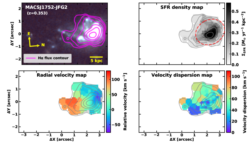
Figure 8: Same as Figure 7 but for MACSJ1752-JFG2.

4.2.2 MACSJ1752-JFG2

In Figure 8, MACSJ1752-JFG2 shows a long tail extending $\sim 25~{}{\rm kpc}$ ($\sim 5\arcsec$ in the angular scale) from the galactic center towards the southern direction. In the ${\rm H\alpha}$ flux distribution, our GMOS/IFU data successfully covers the southern tail except for a few faint blue knots in the outer region. This galaxy also shows two disturbed regions at a galactocentric distance of $\sim 5~{}{\rm kpc}$ towards the south and east directions, exhibiting luminous blue knots. The ${\rm H\alpha}$ flux distribution reproduces these peculiar substructures very well, which is indicative of ongoing star formation in the substructures.

In the SFR surface density map, the “tail” region outside the $1\sigma$ boundary (red dashed ellipse) includes the southern tail and some star-forming knots in the east. This galaxy shows the highest ${\rm H\alpha}$ to ${\rm H\beta}$ ratio among our sample (${\rm H\alpha/H\beta=4.78}$), corresponding to a dust extinction magnitude of $1.61~{}{\rm mag}$. Correcting for dust extinction, we obtain a total SFR of 30.43 $M_{\odot}~{}{\rm yr^{-1}}$ (23.67 $M_{\odot}~{}{\rm yr^{-1}}$ in the disk and 6.76 $M_{\odot}~{}{\rm yr^{-1}}$ in the tail) with a tail SFR fraction of $f_{\rm SFR}=22.2\%$. This indicates that the star formation activity is very strong in both the disk and the tail of this object.

MACSJ1752-JFG2 shows a disk rotation with a maximum rotational velocity of 73.2 ${\rm km~{}s^{-1}}$. It seems that the substructures follow the disk rotation well, but the southern tail shows a high relative velocity of $\sim 100$ ${\rm km~{}s^{-1}}$. This can be a sign of ongoing RPS, indicating that the tail is stripped away from the center of the galaxy.

We obtain the flux-weighted mean of gas velocity dispersion of $\langle\sigma_{v,\rm{gas}}\rangle=43.1~{}{\rm km~{}s^{-1}}$, indicating that this galaxy is dynamically cold as well. The mean velocity dispersions of the disk ($\langle\sigma_{v,\rm{gas}}\rangle=42~{}{\rm km~{}s^{-1}}$) and tail ($\langle\sigma_{v,\rm{gas}}\rangle=47~{}{\rm km~{}s^{-1}}$) do not show a significant difference. However, there is some difference in the velocity dispersion between the two bright knots in the south and east $\sim 5~{}{\rm kpc}$ from the center. The southern large knot shows lower velocity dispersion ($\langle\sigma_{v,\rm{gas}}\rangle\sim 25~{}{\rm km~{}s^{-1}}$) than the eastern one ($\langle\sigma_{v,\rm{gas}}\rangle\sim 50~{}{\rm km~{}s^{-1}}$). This implies that these two knots have different dynamical states, suggesting that ionized gas in the eastern knot is more turbulent than that in the southern one.

4.2.3 A2744-F0083

A2744-F0083 is the most spectacular galaxy, exhibiting numerous star-forming knots outside the main disk and non-ordered tails. There are very bright star-forming knots at both the eastern and western sides of the disk. These knots have comparable sizes and luminosities to compact dwarf galaxies (Owers et al., 2012). The ${\rm H\alpha}$ flux distribution is highly asymmetric, peaking in the eastern region. There are also long tails and extraplanar knots to $\sim 25~{}{\rm kpc}$ ($\sim 5\farcs 5$) towards the southwestern direction from the center, but the ${\rm H\alpha}$ S/N of our GMOS/IFU data is very low in these regions. This is because the observation program of A2744-F0083 used the R400 grating with higher spectral resolution and lower S/N for this galaxy. Thus, we mainly analyze the ionized gas properties of the region within $\sim 10~{}{\rm kpc}$ ($\sim 2\farcs 2$) from the center for this galaxy.

The SFR surface density map shows very strong star formation activity in the disk and in the eastern tail region. Since we remove the AGN contribution to the SFR by subtracting the Voronoi bins with log([N II]$\lambda 6584/{\rm H\alpha})>-0.4$, several bins in the central region are excluded in the map. For dust correction, we obtain a ${\rm H\alpha}$/${\rm H\beta}$ ratio of 4.14 from the AAOmega fiber spectra. The total SFR is 22.00 $M_{\odot}~{}{\rm yr^{-1}}$ with a disk SFR of 14.47 $M_{\odot}~{}{\rm yr^{-1}}$ and a tail SFR of 7.53 $M_{\odot}~{}{\rm yr^{-1}}$ ($f_{\rm SFR}=34.2\%$). The high SFR ratio in the tail indicates that the blue knots in the east undergo vigorous star formation. For comparison, Rawle et al. (2014) estimated the SFR of this galaxy to be 34.2 $M_{\odot}~{}{\rm yr^{-1}}$ based on the sum of the UV and IR luminosities. Different SFR indicators could result in this difference of SFRs because the ${\rm H\alpha}$ luminosity used in this study traces more recent star formation than the UV and IR luminosities (Kennicutt & Evans, 2012).

The radial velocity map shows a clear disk rotation. The maximum rotational velocity is 89.5 ${\rm km~{}s^{-1}}$ in the disk ($R_{\rm disk,c}\sim 1\farcs 4$). Outside the disk, the star-forming knots in the eastern region show a radial velocity of $-88~{}{\rm km~{}s^{-1}}$. The symmetric feature of the radial velocity distribution indicates that the star-forming regions follow the disk rotation well.

In the gas velocity dispersion map, we observe a clear radial gradient from the central disk ($\langle\sigma_{v,\rm{gas}}\rangle=54~{}{\rm km~{}s^{-1}}$) to the tail region ($\langle\sigma_{v,\rm{gas}}\rangle=18~{}{\rm km~{}s^{-1}}$). This is because the ${\rm H\alpha}$ emission lines from the central disk are contaminated by the AGN activity, which broadens the line profiles. This feature has been also shown in the GASP jellyfish galaxies hosting AGNs (Poggianti et al., 2019). Star-forming knots in the tail region are dynamically cold, which is similar to those in MACSJ0916-JFG1 and MACSJ1752-JFG2.

4.2.4 MACSJ1258-JFG1

MACSJ1258-JFG1 is the most massive galaxy ($\log M_{\ast}/M_{\odot}=10.90$) among our sample and hosts a type I AGN. In addition, it has a luminous tail as long as $\sim 10~{}{\rm kpc}$ ($\sim 2\farcs 1$) in the northern region and plenty of blue knots are distributed around the disk. There is also an asymmetric tail feature in the southwestern region of the galaxy. Overall, these substructures seem to be consistent with the ${\rm H\alpha}$ flux distribution of this galaxy.

Like A2744-F0083, the SFR surface density map excludes the central region with the BPT classification of AGN or LINER. We obtain a mean Balmer decrement of 4.64, which corresponds to a $V$-band extinction magnitude of 1.52 mag. We measure a total SFR of 35.71 $M_{\odot}~{}{\rm yr^{-1}}$, with a disk SFR of 18.91 $M_{\odot}~{}{\rm yr^{-1}}$and a tail SFR of 16.80 $M_{\odot}~{}{\rm yr^{-1}}$ ($f_{\rm SFR}=47\%$). The $f_{\rm SFR}$ value is the highest among our targets. This high fraction of the tail SFR might result from strong star formation activity in the substructures in the northern and the southwestern regions ($\sim 10~{}{\rm kpc}$ from the center of the galaxy).

The radial velocity map shows a strong rotation with a maximum rotation velocity of 134.5 ${\rm km~{}s^{-1}}$ in the disk. The northern tail shows a radial velocity of $\sim-100$ ${\rm km~{}s^{-1}}$ and the southern region shows a radial velocity of $\sim 150$ ${\rm km~{}s^{-1}}$. These substructures follow the disk rotation well.

The mean gas velocity dispersion of this galaxy is estimated to be $\langle\sigma_{v,\rm{gas}}\rangle=100.5~{}{\rm km~{}s^{-1}}$, which is higher than those of MACSJ0916-JFG1 and MACSJ1752-JFG2. The mean gas velocity dispersion within the disk is $\langle\sigma_{v,\rm{gas}}\rangle=93.5~{}{\rm km~{}s^{-1}}$, which might be affected by AGN activity like A2744-F0083. The northern tail shows a lower mean velocity dispersion with $\langle\sigma_{v,{\rm gas}}\rangle\sim 50~{}{\rm km~{}s^{-1}}$, whereas the southern region shows a mean gas velocity dispersion of $\langle\sigma_{v,{\rm gas}}\rangle\sim 90~{}{\rm km~{}s^{-1}}$. This indicates that ionized gas in the northern tail is dynamically cold and that in the southern region is more turbulent than the northern region.

4.2.5 MACSJ1720-JFG1

MACSJ1720-JFG1 exhibits interesting substructures such as a bright arc-shaped region at the head of the disk and several blue extraplanar knots in the tail region. The blue knots are located at both the north and south sides of the disk. The ${\rm H\alpha}$ flux map from the GMOS/IFU data reproduces these optical features well.

The SFR surface density map shows that the distribution of star formation activity is strongly concentrated at the the center of the galaxy. We estimated a mean Balmer decrement, obtaining ${\rm H\alpha}$/${\rm H\beta}$$=4.05\pm 1.40$ ($A_{V}=1.09~{}{\rm mag}$). We derive a total SFR of 17.37 $M_{\odot}~{}{\rm yr^{-1}}$, with a disk SFR of 14.09 $M_{\odot}~{}{\rm yr^{-1}}$and a tail SFR of 3.28 $M_{\odot}~{}{\rm yr^{-1}}$ ($f_{\rm SFR}=19\%$).

The radial velocity map shows a clear disk rotation on the axis of the east-west direction. The maximum rotation velocity within the disk is 122.0 ${\rm km~{}s^{-1}}$. The northern tail shows a radial velocity of $\sim 120$ ${\rm km~{}s^{-1}}$ and the blue blob in the southern region shows a radial velocity of $\sim-100$ ${\rm km~{}s^{-1}}$. These disturbed features also rotate following the disk of this galaxy, which is similar to other jellyfish galaxies.

This galaxy shows a mean gas velocity dispersion of $\langle\sigma_{v,\rm{gas}}\rangle=104.5~{}{\rm km~{}s^{-1}}$, which is much higher than those of MACSJ0916-JFG1 and MACSJ1752-JFG2, but similar to that of MACSJ1258-JFG1. This indicates that ionized gas in the star-forming knots of this galaxy seems to be more turbulent than that in the star-forming regions in other jellyfish galaxies. Other shock-heating mechanisms are likely to contribute to the gas ionization in this galaxy, as also suggested by its location in the composite region in the BPT diagram (see Figure 5).

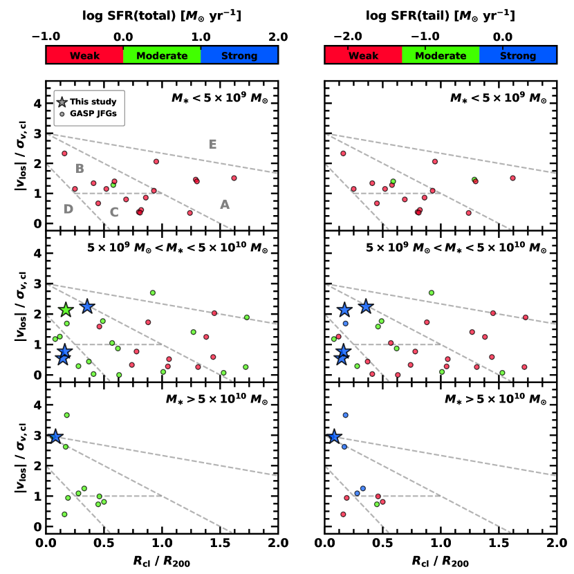
Figure 12: Projected phase-space diagrams of our sample (star symbols) and the GASP jellyfish galaxies (circles). We normalize clustercentric distance ($R_{\rm cl}$) and absolute relative velocity ($|v_{\rm los}|$) with cluster virial radius ($R_{200}$) and velocity dispersion ($\sigma_{v,{\rm cl}}$), respectively. All the data are color-coded by total SFR (left) and tail SFR (right). The color bars on the top denote the logarithmic scale of each SFR. Gray dashed lines represent the boundaries of the five regions that were roughly defined by infall stages of cluster galaxies (Rhee et al., 2017; Mun et al., 2021): Region A (first infall), B (recent infall), C (intemediate infall), D (ancient infall), and E (field). We divide the whole sample into three categories by stellar mass: low-mass ($M_{\ast}<5\times 10^{9}~{}M_{\odot}$; upper), intermediate-mass ($5\times 10^{9}~{}M_{\odot}<M_{\ast}<5\times 10^{10}~{}M_{\odot}$; middle), and high-mass ($M_{\ast}>5\times 10^{10}~{}M_{\odot}$; lower) galaxies.

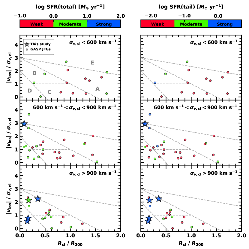
Figure 13: Same as Figure 12, but we divide the sample into three categories by cluster velocity dispersion: low-mass ($\sigma_{v,{\rm cl}}<600~{}{\rm km~{}s^{-1}}$; upper), intermediate-mass ($600~{}{\rm km~{}s^{-1}}<\sigma_{v,{\rm cl}}<900~{}{\rm km~{}s^{-1}}$; middle), and high-mass ($\sigma_{v,{\rm cl}}>900~{}{\rm km~{}s^{-1}}$; lower) clusters.

5 Phase-space Diagrams of the Jellyfish Galaxies

Phase-space diagrams are useful to understand the impact of environmental effects on cluster galaxies concerning their orbital histories (Rhee et al., 2017; Jaffé et al., 2018; Mun et al., 2021). We display the projected phase-space diagrams of our targets and the GASP jellyfish galaxies (Gullieuszik et al., 2020) by categorizing the sample based on stellar mass ( Figure 12) and host cluster velocity dispersion ( Figure 13). Lee et al. (2022) showed the phase-space diagrams of the jellyfish galaxies with different categories of jellyfish morphology. We plot the 2D clustercentric distance normalized by the virial radius of the host cluster ($R_{\rm cl}/R_{200}$) on the x-axis, and we plot the velocity relative to the cluster normalized by the cluster velocity dispersion ($|\Delta v_{\rm los}|/\sigma_{v,{\rm cl}}$) on the y-axis. We measure the line-of-sight velocity of each galaxy with $\Delta v_{\rm los}=c\times(z_{\rm gal}-z_{\rm clu})/(1+z_{\rm clu})$ where $c$ is the speed of light, $z_{\rm gal}$ is the galaxy redshift, and $z_{\rm clu}$ is the cluster redshift.

In Figures 12 and 13, we display total SFRs (left panels) and tail SFRs (right panels) at the top of each panel by categorizing the star formation activity: “weak” (red), “moderate” (green), and “strong” (blue) star formation. Gray dashed lines denote the regions (from A to E) classified in Rhee et al. (2017) and Mun et al. (2021), showing the approximate stages of galaxy infall to the clusters: Region A (first infall), B (recent infall), C (intermediate infall), D (ancient infall), and E (field). In this study, we classify the location of jellyfish galaxies as “inner region” ($R_{\rm cl}/R_{200}\leq 0.5$) and “outer region” ($R_{\rm cl}/R_{200}>0.5$) in their host clusters.

In Figure 12, we plot phase-space diagrams for different bins of galaxy stellar mass: low-mass ($M_{\ast}<5\times 10^{9}~{}M_{\odot}$), intermediate-mass ($5\times 10^{9}~{}M_{\odot}<M_{\ast}<5\times 10^{10}~{}M_{\odot}$), and high-mass ($M_{\ast}>5\times 10^{10}~{}M_{\odot}$). In the low-mass regime, almost all GASP jellyfish galaxies show weak star formation activity (17/18 in total SFR and 16/18 in tail SFR). They are primarily located in the outer region ($R_{\rm cl}/R_{200}>0.5$), with only four of them in the inner region ($R_{\rm cl}/R_{200}\leq 0.5$). Note that no galaxies are located in the ancient infall region, implying that the low-mass jellyfish galaxies might be in the early stages of cluster infall.

In the intermediate-mass regime, the GASP jellyfish galaxies show a wide range of clustercentric distances and velocities in their host clusters. These galaxies are also primarily located in the outer region. Most of them show weak star formation activity in terms of tail SFRs. In contrast, four jellyfish galaxies in this study are located in the inner region of the clusters, and they show moderate or strong star activity. With the combined sample of the GASP survey and this study, this panel shows that the fraction of galaxies with weak star formation activity is higher in the outer region (9/18 in total SFR and 15/18 in tail SFR) than in the inner region (1/12 in total SFR and 4/12 in tail SFR).

In the high-mass regime, there are 10 GASP jellyfish galaxies and MACSJ1258-JFG1 in this study. All massive jellyfish galaxies are located in the inner region of the host clusters. Most of the jellyfish galaxies show moderate or strong star formation activity. The panels in this figure indicates that jellyfish galaxies with higher stellar mass and lower clustercentric distances are likely to exhibit stronger star formation activity on both global (total SFR) and local (tail SFR) scales. This trend has also been observed in Gullieuszik et al. (2020) (see their Figure 4).

In Figure 13, we plot the phase-space diagrams in different bins of cluster velocity dispersion: low-mass hosts ($\sigma_{v,{\rm cl}}<600~{}{\rm km~{}s^{-1}}$), intermediate-mass hosts ($600~{}{\rm km~{}s^{-1}}<\sigma_{v,{\rm cl}}<900~{}{\rm km~{}s^{-1}}$), and high-mass hosts ($\sigma_{v,{\rm cl}}>900~{}{\rm km~{}s^{-1}}$). For the low-mass host clusters, half of the 14 GASP galaxies are located outside the virial radius. A majority of the jellyfish galaxies show weak star formation activity, but galaxies in the inner region mostly show stronger star formation activity than those in the outer region. This trend can be also seen in intermediate-mass host clusters. Most galaxies in the outer region show weak star formation activity (9/11 in total and tail SFR), whereas those in the inner region have a lower fraction of weak star formation activity (4/16 in total SFR and 9/16 in tail SFR). For the high-mass host clusters, there are 14 GASP jellyfish galaxies and 4 galaxies in this study. In terms of total SFRs, the fraction of galaxies with moderate and strong star formation activity (12/18) is higher in high-mass clusters than in low-mass (6/14) and intermediate-mass (13/27) clusters. This trend is also seen with tail SFRs: 3/14 in low-mass, 9/27 in intermediate-mass, and 8/18 in high-mass clusters. This indicates that the star formation activity of jellyfish galaxies in high-mass clusters is likely to be more enhanced compared to those in low-mass and intermediate-mass clusters. In addition, there are no GASP galaxies located in the first infall region (“A”) in these massive clusters in contrast to low- and intermediate-mass clusters. This implies that the jellyfish galaxies in massive clusters are at a later phase of cluster infall than in low-mass clusters.

Combining the GASP sample and our sample, these phase-space diagrams reveal the following. First, our jellyfish galaxy sample is located in the inner region with a wide range of relative velocities. Second, it is clearly shown that jellyfish galaxies in the inner region tend to have higher SFRs than those in the outer region. Third, the star formation activity of jellyfish galaxies tends to increase as galaxy stellar mass increases, as shown in Figure 12. This reflects the SFR-mass relation of jellyfish galaxies as also shown in Figure 2 and 4 in Lee et al. (2022).

Finally, the star formation activity of jellyfish galaxies tend to increase as the host cluster velocity dispersion increases, as shown in Figure 13. In this context, Lee et al. (2022) revealed that jellyfish galaxies with strong RPS signatures show more enhanced star formation activity in more massive clusters with a higher degree of RPS.

6 Summary

In this study, we presented an observational study of the five jellyfish galaxies in the MACS clusters and Abell 2744 at $z>0.3$ based on Gemini GMOS/IFU observations. Using these data, we investigated the ionized gas properties of these jellyfish galaxies such as ionization mechanisms, kinematics, and SFRs. Lee et al. (2022) also used the ${\rm H\alpha}$-derived SFRs in this study and suggested positive correlations between the star formation activity of jellyfish galaxies and their host cluster properties. Our main results can be summarized as follows.

1. The BPT diagrams of [O III]$\lambda$5007/${\rm H\beta}$ and [N II]$\lambda$6584/${\rm H\alpha}$ show that the five jellyfish galaxies have different ionization mechanisms. MACSJ0916-JFG1 and MACSJ1752-JFG2 are located in the star-forming region, indicating that the gas contents in these galaxies are ionized purely by star formation. On the other hand, A2744-F0083 and MACSJ1258-JFG1 are located in the AGN region with high line ratios of [O III]$\lambda$5007/${\rm H\beta}$ and [N II]$\lambda$6584/${\rm H\alpha}$. MACSJ1720-JFG1 is located in the composite region, implying a mixed contribution of star formation and other shock-heating mechanisms.

2. The spatial distributions of the ${\rm H\alpha}$ flux are well-matched with the optical features in all five jellyfish galaxies. This indicates that the ionized gas distribution is consistent with that of the stellar light distribution in the jellyfish galaxies.

3. The radial velocity distributions of the jellyfish galaxies indicate that ionized gas in the disk and tail regions rotates around the center of each galaxy. Some tail regions (e.g. eastern side of MACSJ1752-JFG2) show high relative velocities with respect to the center of the galaxy, which indicates signs of RPS.

4. MACSJ0916-JFG1, MACSJ1752-JFG2 and the tail regions in A2744-F0083 and MACSJ1258-JFG1 show a mean velocity dispersion lower than $50~{}{\rm km~{}s^{-1}}$, which is consistent with the mean value of star-forming clumps in the GASP jellyfish galaxies. This implies that the ionized gas in those regions is dynamically cold. In contrast, MACSJ1720-JFG1 and the central regions in A2744-F0083 and MACSJ1258-JFG1 show mean velocity dispersions higher than $50~{}{\rm km~{}s^{-1}}$, indicating that the ionized gas is more turbulent than typical star-forming regions. This could be associated with the AGN activity or other shock-heating mechanisms.

5. The total and tail SFRs of the five jellyfish galaxies are much higher than those of the GASP sample. The median SFRs of our targets are 22.0 $M_{\odot}~{}{\rm yr^{-1}}$ in total and 6.8 $M_{\odot}~{}{\rm yr^{-1}}$ in the tails, whereas those of the GASP sample are 1.1 $M_{\odot}~{}{\rm yr^{-1}}$ in total and 0.03 $M_{\odot}~{}{\rm yr^{-1}}$ in the tails. In addition, the median SFR fraction in the tail ($f_{\rm SFR}$) is also much higher in this study ($f_{\rm SFR}=22\%$) than in the GASP studies ($f_{\rm SFR}=3\%$).

6. In the projected phase-space diagrams, the jellyfish galaxies in this study are located in the inner region with a wide range of orbital velocities relative to the cluster center. Combining the GASP sample and our sample, we find that jellyfish galaxies with higher stellar masses and higher host cluster velocity dispersions are more likely to be located in the inner region of the clusters with more enhanced star formation activity.

We thank the anonymous referee for his/her important comments and suggestions to improve the submitted manuscript. This study was supported by the National Research Foundation grant funded by the Korean Government (NRF-2019R1A2C2084019). This work was supported by K-GMT Science Program (PID: GS-2019A-Q-214, GN-2019A-Q-215, GS-2019B-Q-219, and GN-2021A-Q-205) of Korea Astronomy and Space Science Institute (KASI). Based on observations obtained at the international Gemini Observatory, a program of NSF’s NOIRLab, acquired through the Gemini Observatory Archive at NSF’s NOIRLab and processed using the Gemini IRAF package, which is managed by the Association of Universities for Research in Astronomy (AURA) under a cooperative agreement with the National Science Foundation on behalf of the Gemini Observatory partnership: the National Science Foundation (United States), National Research Council (Canada), Agencia Nacional de Investigación y Desarrollo (Chile), Ministerio de Ciencia, Tecnología e Innovación (Argentina), Ministério da Ciência, Tecnologia, Inovações e Comunicações (Brazil), and Korea Astronomy and Space Science Institute (Republic of Korea). This research has made use of the NASA/IPAC Extragalactic Database (NED), which is operated by the Jet Propulsion Laboratory, California Institute of Technology, under contract with the National Aeronautics and Space Administration. This research is based on observations made with the NASA/ESA Hubble Space Telescope and the Galaxy Evolution Explorer obtained from the Mikulski Archive for Space Telescopes (MAST) data archive at the Space Telescope Science Institute (STScI). STScI is operated by the Association of Universities for Research in Astronomy, Inc., under NASA contract NAS 5-26555. This publication makes use of data products from the Wide-field Infrared Survey Explorer, which is a joint project of the University of California, Los Angeles, and the Jet Propulsion Laboratory/California Institute of Technology, funded by the National Aeronautics and Space Administration. This work is based in part on observations made with the Spitzer Space Telescope, which was operated by the Jet Propulsion Laboratory, California Institute of Technology under a contract with NASA.

References

- Astropy Collaboration et al. (2013) Astropy Collaboration, Robitaille, T. P., Tollerud, E. J., et al. 2013, A&A, 558, A33. doi:10.1051/0004-6361/201322068
- Astropy Collaboration et al. (2018) Astropy Collaboration, Price-Whelan, A. M., Sipőcz, B. M., et al. 2018, AJ, 156, 123. doi:10.3847/1538-3881/aabc4f
- Baldwin et al. (1981) Baldwin, J. A., Phillips, M. M., & Terlevich, R. 1981, PASP, 93, 5. doi:10.1086/130766
- Bekki (2009) Bekki, K. 2009, MNRAS, 399, 2221. doi:10.1111/j.1365-2966.2009.15431.x
- Bellhouse et al. (2017) Bellhouse, C., Jaffé, Y. L., Hau, G. K. T., et al. 2017, ApJ, 844, 49. doi:10.3847/1538-4357/aa7875
- Bellhouse et al. (2019) Bellhouse, C., Jaffé, Y. L., McGee, S. L., et al. 2019, MNRAS, 485, 1157. doi:10.1093/mnras/stz460
- Bertin & Arnouts (1996) Bertin, E. & Arnouts, S. 1996, A&AS, 117, 393. doi:10.1051/aas:1996164
- Boschin et al. (2006) Boschin, W., Girardi, M., Spolaor, M., et al. 2006, A&A, 449, 461. doi:10.1051/0004-6361:20054408
- Boselli et al. (2016) Boselli, A., Cuillandre, J. C., Fossati, M., et al. 2016, A&A, 587, A68. doi:10.1051/0004-6361/201527795
- Boselli et al. (2019) Boselli, A., Epinat, B., Contini, T., et al. 2019, A&A, 631, A114. doi:10.1051/0004-6361/201936133
- Bradley et al. (2021) Bradley L., et al., 2019, astropy/photutils: v1.0.2, doi:10.5281/zenodo.2533376
- Cappellari & Copin (2003) Cappellari, M. & Copin, Y. 2003, MNRAS, 342, 345. doi:10.1046/j.1365-8711.2003.06541.x
- Cardelli et al. (1989) Cardelli, J. A., Clayton, G. C., & Mathis, J. S. 1989, ApJ, 345, 245. doi:10.1086/167900
- Castignani et al. (2020) Castignani, G., Combes, F., & Salomé, P. 2020, A&A, 635, L10. doi:10.1051/0004-6361/201937155
- Chabrier (2003) Chabrier, G. 2003, PASP, 115, 763. doi:10.1086/376392
- Chung et al. (2009) Chung, A., van Gorkom, J. H., Kenney, J. D. P., et al. 2009, AJ, 138, 1741. doi:10.1088/0004-6256/138/6/1741
- Cortese et al. (2007) Cortese, L., Marcillac, D., Richard, J., et al. 2007, MNRAS, 376, 157. doi:10.1111/j.1365-2966.2006.11369.x
- Dressler (1980) Dressler, A. 1980, ApJ, 236, 351. doi:10.1086/157753
- Durret et al. (2021) Durret, F., Chiche, S., Lobo, C., et al. 2021, A&A, 648, A63. doi:10.1051/0004-6361/202039770
- Ebeling et al. (2001) Ebeling, H., Edge, A. C., & Henry, J. P. 2001, ApJ, 553, 668. doi:10.1086/320958
- Ebeling et al. (2010) Ebeling, H., Edge, A. C., Mantz, A., et al. 2010, MNRAS, 407, 83. doi:10.1111/j.1365-2966.2010.16920.x
- Ebeling et al. (2014) Ebeling, H., Stephenson, L. N., & Edge, A. C. 2014, ApJ, 781, L40. doi:10.1088/2041-8205/781/2/L40
- Ebeling et al. (2017) Ebeling, H., Qi, J., & Richard, J. 2017, MNRAS, 471, 3305. doi:10.1093/mnras/stx1636
- Eskew et al. (2012) Eskew, M., Zaritsky, D., & Meidt, S. 2012, AJ, 143, 139. doi:10.1088/0004-6256/143/6/139
- Evrard et al. (2008) Evrard, A. E., Bialek, J., Busha, M., et al. 2008, ApJ, 672, 122. doi:10.1086/521616
- Foreman-Mackey et al. (2013) Foreman-Mackey, D., Hogg, D. W., Lang, D., et al. 2013, PASP, 125, 306. doi:10.1086/670067
- Golovich et al. (2019) Golovich, N., Dawson, W. A., Wittman, D. M., et al. 2019, ApJS, 240, 39. doi:10.3847/1538-4365/aaf88b
- Gullieuszik et al. (2020) Gullieuszik, M., Poggianti, B. M., McGee, S. L., et al. 2020, ApJ, 899, 13. doi:10.3847/1538-4357/aba3cb
- Gunawardhana et al. (2011) Gunawardhana, M. L. P., Hopkins, A. M., Sharp, R. G., et al. 2011, MNRAS, 415, 1647. doi:10.1111/j.1365-2966.2011.18800.x
- Gunn & Gott (1972) Gunn, J. E. & Gott, J. R. 1972, ApJ, 176, 1. doi:10.1086/151605
- Harris et al. (2020) Harris, C.R., Millman, K.J., van der Walt, S.J. et al. Array programming with NumPy. Nature 585, 357–362 (2020). https://doi.org/10.1038/s41586-020-2649-2
- Hester et al. (2010) Hester, J. A., Seibert, M., Neill, J. D., et al. 2010, ApJ, 716, L14. doi:10.1088/2041-8205/716/1/L14
- Hopkins et al. (2003) Hopkins, A. M., Miller, C. J., Nichol, R. C., et al. 2003, ApJ, 599, 971. doi:10.1086/379608
- Hunter (2007) Hunter, J. D. 2007, Computing in Science and Engineering, 9, 90. doi:10.1109/MCSE.2007.55
- Jaffé et al. (2018) Jaffé, Y. L., Poggianti, B. M., Moretti, A., et al. 2018, MNRAS, 476, 4753. doi:10.1093/mnras/sty500
- Kalita & Ebeling (2019) Kalita, B. S. & Ebeling, H. 2019, ApJ, 887, 158. doi:10.3847/1538-4357/ab5184
- Kauffmann et al. (2003) Kauffmann, G., Heckman, T. M., Tremonti, C., et al. 2003, MNRAS, 346, 1055. doi:10.1111/j.1365-2966.2003.07154.x
- Kennicutt (1998) Kennicutt, R. C. 1998, ARA&A, 36, 189. doi:10.1146/annurev.astro.36.1.189
- Kennicutt & Evans (2012) Kennicutt, R. C. & Evans, N. J. 2012, ARA&A, 50, 531. doi:10.1146/annurev-astro-081811-125610
- Kewley et al. (2001) Kewley, L. J., Dopita, M. A., Sutherland, R. S., et al. 2001, ApJ, 556, 121. doi:10.1086/321545
- Larson et al. (1980) Larson, R. B., Tinsley, B. M., & Caldwell, C. N. 1980, ApJ, 237, 692. doi:10.1086/157917
- Lee et al. (2022) Lee, J. H., Lee, M. G., Mun, J. Y., et al. 2022, ApJ, 931, L22. doi:10.3847/2041-8213/ac6e39
- Lee & Jang (2016) Lee, M. G. & Jang, I. S. 2016, ApJ, 819, 77. doi:10.3847/0004-637X/819/1/77
- Lotz et al. (2017) Lotz, J. M., Koekemoer, A., Coe, D., et al. 2017, ApJ, 837, 97. doi:10.3847/1538-4357/837/1/97
- McPartland et al. (2016) McPartland, C., Ebeling, H., Roediger, E., et al. 2016, MNRAS, 455, 2994. doi:10.1093/mnras/stv2508
- Medezinski et al. (2018) Medezinski, E., Battaglia, N., Umetsu, K., et al. 2018, PASJ, 70, S28. doi:10.1093/pasj/psx128
- Medling et al. (2018) Medling, A. M., Cortese, L., Croom, S. M., et al. 2018, MNRAS, 475, 5194. doi:10.1093/mnras/sty127
- Moore et al. (1996) Moore, B., Katz, N., Lake, G., et al. 1996, Nature, 379, 613. doi:10.1038/379613a0
- Moretti et al. (2022) Moretti, A., Radovich, M., Poggianti, B. M., et al. 2022, ApJ, 925, 4. doi:10.3847/1538-4357/ac36c7
- Mun et al. (2021) Mun, J. Y., Hwang, H. S., Lee, M. G., et al. 2021, Journal of Korean Astronomical Society, 54, 17. doi:10.5303/JKAS.2021.54.1.17
- Osato et al. (2020) Osato, K., Shirasaki, M., Miyatake, H., et al. 2020, MNRAS, 492, 4780. doi:10.1093/mnras/staa117
- Owen et al. (2006) Owen, F. N., Keel, W. C., Wang, Q. D., et al. 2006, AJ, 131, 1974. doi:10.1086/500573
- Owers et al. (2011) Owers, M. S., Randall, S. W., Nulsen, P. E. J., et al. 2011, ApJ, 728, 27. doi:10.1088/0004-637X/728/1/27
- Owers et al. (2012) Owers, M. S., Couch, W. J., Nulsen, P. E. J., et al. 2012, ApJ, 750, L23. doi:10.1088/2041-8205/750/1/L23
- Poggianti et al. (2016) Poggianti, B. M., Fasano, G., Omizzolo, A., et al. 2016, AJ, 151, 78. doi:10.3847/0004-6256/151/3/78
- Poggianti et al. (2017) Poggianti, B. M., Moretti, A., Gullieuszik, M., et al. 2017, ApJ, 844, 48. doi:10.3847/1538-4357/aa78ed
- Poggianti et al. (2019) Poggianti, B. M., Gullieuszik, M., Tonnesen, S., et al. 2019, MNRAS, 482, 4466. doi:10.1093/mnras/sty2999
- Rawle et al. (2014) Rawle, T. D., Altieri, B., Egami, E., et al. 2014, MNRAS, 442, 196. doi:10.1093/mnras/stu868
- Repp & Ebeling (2018) Repp, A. & Ebeling, H. 2018, MNRAS, 479, 844. doi:10.1093/mnras/sty1489
- Rhee et al. (2017) Rhee, J., Smith, R., Choi, H., et al. 2017, ApJ, 843, 128. doi:10.3847/1538-4357/aa6d6c
- Rich et al. (2011) Rich, J. A., Kewley, L. J., & Dopita, M. A. 2011, ApJ, 734, 87. doi:10.1088/0004-637X/734/2/87