Influence of fine structures on gyrosynchrotron emission of flare loops modulated by sausage modes

Abstract

Sausage modes are one leading mechanism for interpreting short period quasi-periodic pulsations (QPPs) of solar flares. Forward modeling their radio emission is crucial for identifying sausage modes observationally and for understanding their connections with QPPs. Using the numerical output from three-dimensional magnetohydrodynamic (MHD) simulations, we forward model the gyrosynchrotron (GS) emission of flare loops modulated by sausage modes and examine the influence of loop fine structures. The temporal evolution of the emission intensity is analyzed for an oblique line of sight crossing the loop center. We find that the low- and high-frequency intensities oscillate in-phase at the period of sausage modes for models with or without fine structures. For low-frequency emissions where the optically thick regime arises, the modulation magnitude of the intensity is dramatically reduced by the fine structures at some viewing angles. On the contrary, for high-frequency emissions where the optically thin regime holds, the effect of fine structures or viewing angle is marginal. Our results show that the periodic intensity variations of sausage modes are not wiped out by the fine structures, and sausage modes remains a promising candidate mechanism for QPPs even when flare loops are fine-structured.

1 Introduction

Quasi-periodic pulsations (QPPs) refer broadly to the oscillatory intensity variations commonly observed in solar flare emissions across a broad range of passbands (see the reviews by, e.g., Nakariakov & Melnikov, 2009; Kupriyanova et al., 2020). In spite of the abundant observed instances, the physical mechanisms responsible for QPPs still remain inconclusive (Van Doorsselaere et al., 2016; Zimovets et al., 2021). Sausage modes can cause periodic compression and rarefaction of flare loops and are thus thought of as one of the mechanisms accounting for QPPs in solar flares (see the recent review by Li et al., 2020). In terms of observations, candidate sausage modes have been reported in the radio band (e.g., Melnikov et al., 2005; Kolotkov et al., 2015), in the extreme-ultraviolet (EUV) (e.g., Su et al., 2012; Tian et al., 2016), as well as in X-ray (e.g., Zimovets & Struminsky, 2010).

The classical theory of sausage modes (Edwin & Roberts, 1983) assumes that sausage modes are supported by an axisymmetric monolithic loop. However, high resolution observations (e.g., Brooks et al., 2012; Cirtain et al., 2013; Peter et al., 2013; Aschwanden & Peter, 2017) suggest that coronal loops are fine-structured or multi-stranded. Multi-stranded loop models have been invoked to explain such observations as the coronal fuzziness (Tripathi et al., 2009; Guarrasi et al., 2010) and the time lag of EUV light curves (Warren et al., 2003; Viall & Klimchuk, 2012). Transverse kink oscillations in multi-stranded loops have attracted substantial attention in both analytical studies (e.g., Luna et al., 2008; Van Doorsselaere et al., 2008; Luna et al., 2010) and MHD simulations (e.g., Terradas et al., 2008; Ofman, 2009; Pascoe et al., 2011; Magyar & Van Doorsselaere, 2016; Guo et al., 2019). For flare loops, fine strands tend to be common to see as well (e.g., Zimovets et al., 2013; Tian et al., 2016). This led Guo et al. (2021, hereafter G21) to examine the influence of fine structures on sausage modes in flare loops, the primary conclusion being that the global sausage mode is still identifiable in spite of the loop fine structures.

One key question to answer is then whether the fine structures can influence the emissions from multi-stranded flare loops experiencing sausage perturbations. This issue is particularly necessary to address for the radio band, where high temporal resolution can be achieved. For solar radio emissions, the gyrosynchrotron (GS) emission is known to dominate at the millimeter and centimeter wavelengths (Bastian et al., 1998). GS emissions of flare loops can be modulated by the sausage modes therein. In turn, these modulations also provide signatures for identifying the sausage modes in flare loops. Along this line of thinking, a variety of forward modeling analyses with different levels of sophistication have been performed, from the model where a homogeneous emission source was assumed (e.g., Nakariakov & Melnikov, 2006; Reznikova et al., 2007; Fleishman et al., 2008; Mossessian & Fleishman, 2012), to the models where inhomogeneity (e.g., Reznikova et al., 2014, 2015) or loop curvature (e.g., Kuznetsov et al., 2015) was taken into account.

In this work, we forward model the GS emission of flare loops modulated by sausage modes. New is that we take into account the fine structures of flare loops and examine the influence of fine structures on the GS emission. Section 2 shows the numerical model. In Sections 3 and 4 we present the forward modeling results. Section 5 summarizes this study.

2 Numerical Model

The MHD model that we use for forward modeling purposes was described by G21, where three-dimensional time-dependent simulations were performed to examine how fast sausage modes are influenced by fine structures in straight, field-aligned, flare loops. Two MHD models, to be labeled ‘noFS’ and ‘FS’, were constructed in G21. For both models, the equilibrium magnetic field $\mathbf{B}$ is $z$-directed, and all equilibrium quantities are $z$-independent. For model noFS, the loop is axisymmetric with its density prescribed by

$$\rho_{\rm noFS}=\rho_{\rm e}+(\rho_{\rm i}-\rho_{\rm e})f(x,y),$$ (1)

where $[\rho_{\rm i},\rho_{\rm e}]$=$[5\times 10^{10},0.8\times 10^{9}]m_{p}~{}{\rm cm}^{-3}$ represent the mass densities at the loop axis and infinitely far from the loop, respectively. In addition, $m_{p}$ is the proton mass. A function $f(x,y)={\rm exp}[-(r/R)^{\alpha}]$ is used to control the density profile, with $r=\sqrt{x^{2}+y^{2}}$, $\alpha=5$, and the nominal loop radius $R=5$ Mm. The temperature distribution follows the same functional form as the density, with the temperature at the loop axis being $T_{i}=10$ MK and that far from the loop being $T_{e}=2$ MK. The magnetic field ($B_{z}$) is prescribed in such a way that transverse force balance is maintained, and the resulting $B_{z}$ increases from $50$ G at the axis to $77.3$ G far from the loop. The length of the flare loop is $L=45$ Mm.

Model FS modifies model noFS by introducing fine structures as randomly distributed, small-scale, density variations to the loop interior,

$$\rho_{\rm FS}(x,y)=\rho_{\rm noFS}(x,y)+(\rho_{\rm i}-\rho_{\rm e})f(x,y)g(x,y),$$ (2)

where

$$g(x,y)=\frac{\sum_{j=1}^{N_{\rm FS}}[{\rm exp}(-\bar{r}_{j}^{\alpha}){\rm cos}(\pi\bar{r}_{j})]}{|\sum_{j=1}^{N_{\rm FS}}[{\rm exp}(-\bar{r}_{j}^{\alpha}){\rm cos}(\pi\bar{r}_{j})]|_{\rm max}},$$ (3)

with

$$\bar{r}_{j}=\frac{\sqrt{(x-x_{j})^{2}+(y-y_{j})^{2}}}{R_{\rm FS}}.$$ (4)

In the above equations, $R_{\rm FS}=0.8$ Mm is the nominal radius of fine strands, and $[x_{j},y_{j}]$ represents the randomly generated position for an individual strand. We take the number of fine structure to be $N_{\rm FS}=20$. The temperature profile remains unchanged relative to model noFS, whereas the magnetic field strength $B_{z}$ is adjusted to ensure transverse force balance. Figure 1 displays how the thermal electron density is distributed in the $x-y$ plane (the left column) and the $y-z$ cut through $x=0$ (right) for both model noFS (the upper row) and model FS (lower). When computing the GS emission, we assume that nonthermal electrons exist only inside the loop, namely in the cylinder with the nominal loop radius. We restrict ourselves to a line of sight (LoS) that is in the $x=0$ plane and makes an angle of $45^{\circ}$ with the $z$-axis. Consequently, only the red-lined segments in Figure 1 are of interest, and they are $\sim 14$ Mm in length. However, we distinguish between two orientations where the observer on the Earth is placed at the opposite directions. We refer to the two situations as “LoS+” and “LoS-”, respectively. The coordinate along a LoS, $z^{\prime}$, increases away from the observer.

The system in both models is perturbed by a radially directed axisymmetric initial velocity prescribed by

$$v_{x}(x,y,z;t=0)=v_{0}\frac{r}{\sigma_{r}}{\rm exp}\left[\frac{1}{2}\left(1-\frac{r^{2}}{\sigma_{r}^{2}}\right)\right]{\rm sin}\left(\frac{\pi z}{L}\right)\left(\frac{x}{r}\right)$$ (5)

and

$$v_{y}(x,y,z;t=0)=v_{0}\frac{r}{\sigma_{r}}{\rm exp}\left[\frac{1}{2}\left(1-\frac{r^{2}}{\sigma_{r}^{2}}\right)\right]{\rm sin}\left(\frac{\pi z}{L}\right)\left(\frac{y}{r}\right),$$ (6)

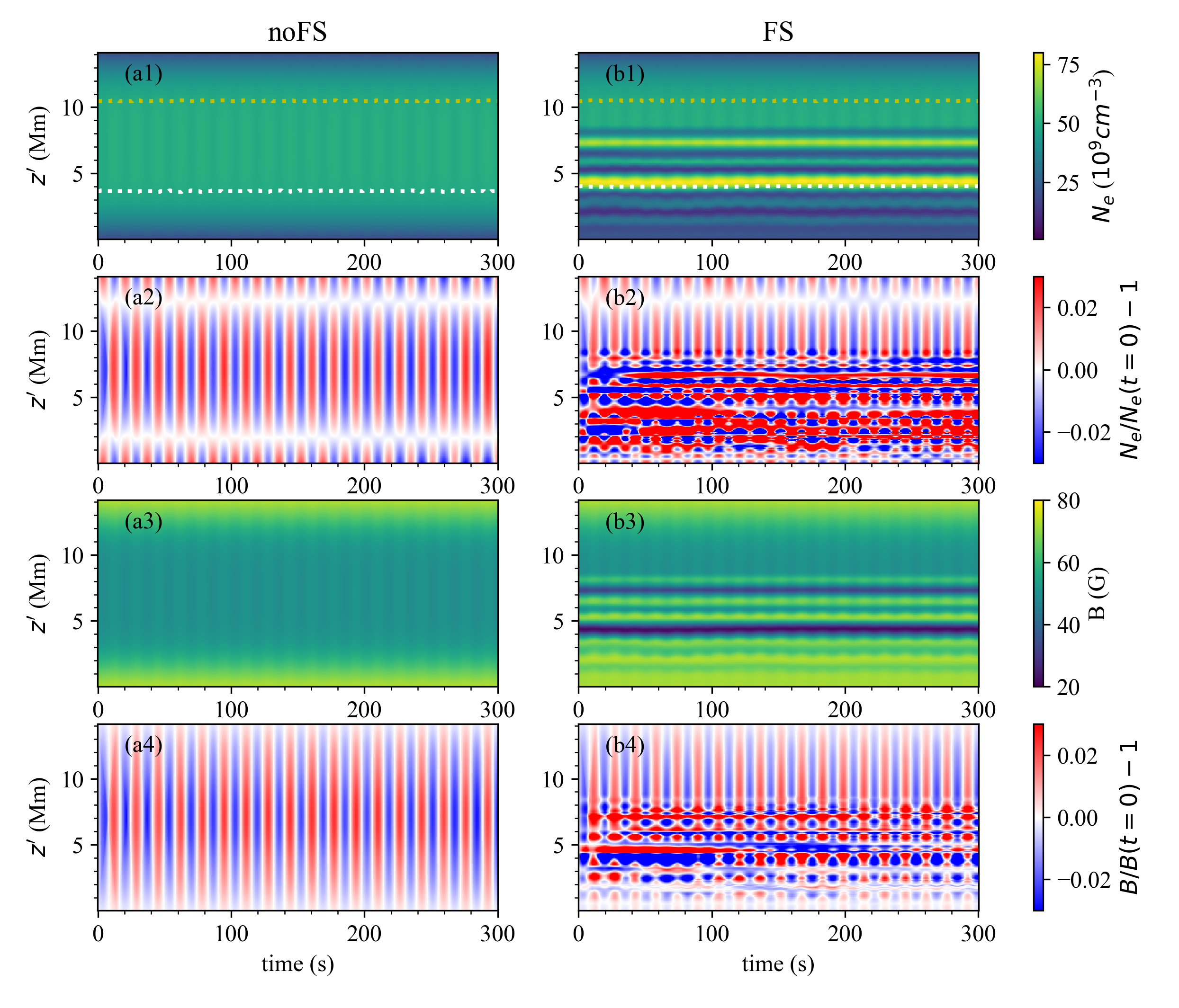
Figure 2: Left: Temporal variations of (a1) the electron number density ($N_{e}$), (a2) the relative variation of $N_{e}$, (a3) the magnetic field strength ($B$), and (a4) the relative variation of $B$ along the LoS for model noFS. Right: Same as left but for model FS. The dotted curves in (a1) and (b1) mark the locations where the optical depth of the 2.5 GHz emission reaches unity for LoS+ (white) and LoS- (yellow).

where $v_{0}=10{\rm~{}km~{}s^{-1}}$ is the velocity amplitude, and $\sigma_{r}=5$ Mm characterizes the spatial extent of the initial perturbation. An axial fundamental sausage oscillation is established in both models, despite the transverse fine structuring in model FS. The fine strands nonetheless experience some kink-like motion (see G21 for details). Figure 2 shows the thermal electron number density ($N_{e}$) and the magnetic field strength ($B$) as functions of $z^{\prime}$ and $t$ at orientation LoS+ for both model noFS (the left column) and model FS (right). The variations of $N_{e}$ and $B$ relative to the equilibrium values (at $t=0$) are also given. One sees for model noFS that the temporal variations of $B$ at all $z^{\prime}$ are in-phase, whereas those of $N_{e}$ outside the interval $2~{}{\rm Mm}\lesssim z^{\prime}\lesssim~{}12~{}{\rm Mm}$ are in anti-phase with the variations in this interval. Moving on to model FS, one still readily discerns periodic variations in both $N_{e}$ and $B$. In fact, their profiles for $z^{\prime}\gtrsim~{}8$ Mm are strikingly similar to what happens in model noFS. The most obvious differences between the two models lie in the range $z^{\prime}\lesssim~{}8$ Mm where fine structures are present and move in a rather complicated manner. These fine structures may move back and forth along the LoS in response to the dominant sausage oscillation. Occasionally, they may deviate away from the LoS as a result of their kink-like behavior as well.

3 Gyrosynchrotron Emission: Reference Computations

We compute GS emission using the fast GS code (FGS) developed by Kuznetsov et al. (2011) (see also Fleishman & Kuznetsov 2010). In short, FGS computes the local values of the absorption coefficient and emissivity, thereby accounting for inhomogeneous sources by integrating the radiative transfer equation. Similar to Reznikova et al. (2014), we assume that the number density of nonthermal electrons ($N_{b}$) is proportional to the thermal one ($N_{e}$), and specifically takes the form $N_{b}=0.005N_{e}$. Here the constant of proportionality is such that the resulting $N_{b}$ is compatible with observations of typical flares (e.g., Fleishman et al., 2022). The spectral index of nonthermal electrons is $\delta=3.5$, with the energy range being $0.1$ to $10$ MeV. The pitch angle distribution of nonthermal electrons is taken to be isotropic. We assume that both LoS+ and LoS- thread a beam with a cross-sectional area of 48 km$\times$48 km when projected onto the plane of sky, in view of the spatial resolution that the Atacama Large Millimeter/submillimeter Array (ALMA) can achieve (Wedemeyer et al., 2016).

Figure 3 shows (a) the number density of nonthermal electrons $N_{b}$, (b) the magnetic field strength $B$, and (c) the Razin frequency $f_{R}$ as a function of $z^{\prime}$ at $t=0$ for orientation LoS+ for both model noFS (the orange curves) and model FS (blue). The pertinent profiles for orientation LoS- can be readily deduced. Here $f_{R}$ is evaluated as $20N_{e}/|B_{\perp}|$ (in CGS units, see Reznikova et al., 2014), with $B_{\perp}$ being the instantaneous $B$ component transverse to the LoS. The relevance of $f_{R}$ is that, when the thermal electron density is high, the spectral peak of GS emission is formed due to the Razin effect, which considerably suppresses the intensity at frequencies below $f_{R}$ (Razin, 1960). Figure 3d shows the spectral profiles for model noFS (the orange curve) and model FS (blue) at $t=0$. We discriminate the profiles for LoS+ and LoS- by the solid and dash-dotted curves only for model FS. For model noFS, the results are identical at both orientations due to the symmetry of this LoS. Both the spectral profile and the peak frequency of model FS are different from the results of model noFS. These differences are caused by the physical parameters (e.g., Figures 3a, 3b) and Razin frequencies (Figure 3c) along the LoS. Observing the loop at LoS+ or LoS- for model FS, one sees that the intensity does not change at high frequencies, but changes at low frequencies. Figure 3e shows the optical depth $\tau$ as a function of frequency $f$ at $t=0$ for both models. Here $\tau$ is obtained by integrating the local $\varkappa$ along the LoS, with $\varkappa$ being the average of the absorption coefficients of the X and O modes weighted by their local intensities. Similar to Figure 3(d), we discriminate $\tau$ of LoS+ and LoS- only for model FS, though we do not see any substantial difference for the two orientations. From Figure 3(e), one sees that at frequencies $f\gtrsim 5$ GHz, the optical depth is less than unity and thus the loop is optically thin for both models.

Figure 4 shows the temporal evolution of intensity (left column) and the variations with respect to $t=0$ (right), taking the results at five frequencies as examples. For model noFS (top row), the intensities at all frequencies, including the optically thick 2.5 GHz, oscillate in phase at the period of sausage mode. The result that low and high frequency emissions oscillate in-phase when the Razin effect dominates agrees with that of Reznikova et al. (2007) and Mossessian & Fleishman (2012) where a homogeneous emission source was assumed. This result also agrees with Reznikova et al. (2014) at some viewing angles when an inhomogeneous emission source was examined. At high frequencies, the loop is optically thin, thus every voxel along the LoS contributes to the total emission, making the intensity variation follow the oscillation of the global sausage mode. At low frequencies (e.g., 2.5 GHz), however, the loop is optically thick, so the emission mostly comes from the volume where the optical depth is about unity (see the dotted lines in Figure 2). It is inappropriate to compare our results with the approximate formula proposed by Dulk & Marsh (1982), where the Razin effect was not considered. Furthermore, the physical parameters vary smoothly at the loop boundary, making the intensity of the optically thick emission more difficult to estimate using these approximate formula. For model FS (middle and bottom rows), the intensities at all frequencies also oscillate in-phase. The most striking difference, relative to model noFS, is the relative intensity variation of $2.5$ GHz. The modulation amplitude at this frequency is reduced by the fine structures, with the reduction being more significant for LoS+. This effect is attributed to the optical thickness. In the optically thick regime, the intensity is dominated by the layer where the optical depth reaches unity, thus the fine structures or the orientation observing them would influence the intensity and its variation. At high frequencies, the intensity variations are not obviously influenced by the fine structures or the viewing angle.

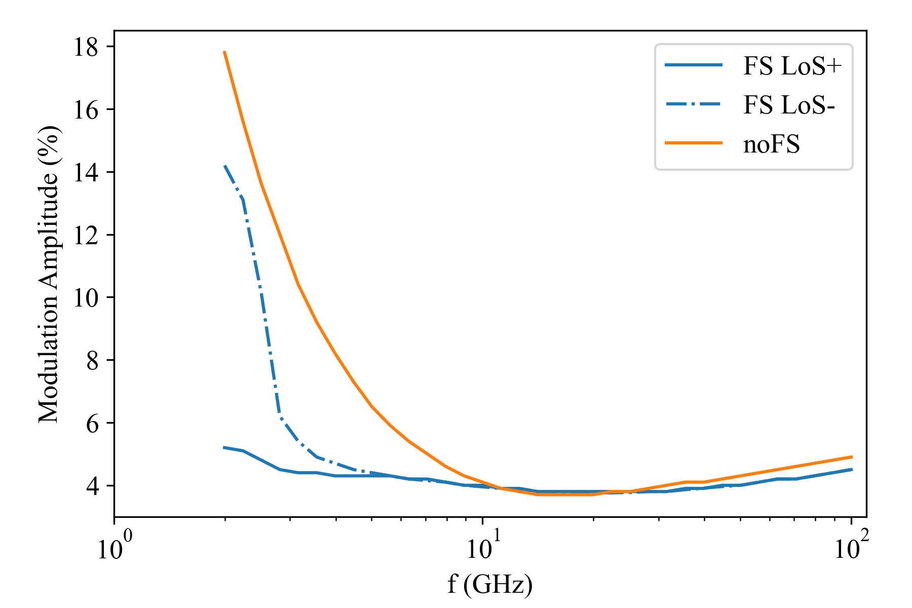
Figure 5: Modulation amplitudes at different frequencies for models FS and noFS.

Figure 5 plots the modulation amplitude as a function of frequency for both models. We obtain the modulation amplitude at each frequency by fitting the relative variation (the right column in Figure 4) with a sinusoidal curve. For model noFS, the modulation amplitude reaches its minimum around the peak frequency, and increases rapidly with decreasing frequency, consistent with the results of Mossessian & Fleishman (2012) and Kuznetsov et al. (2015). For model FS, the modulation amplitudes at low frequencies are dramatically reduced, with the effect being more pronounced for LoS+. At high frequencies, the modulation amplitudes are not obviously influenced by the fine structures. This effect is also due to different optical depths at different frequencies. As an example, we plot in Figure 2 the positions where the optical depth of the 2.5 GHz emission reaches unity for LoS+ (the white curves) and LoS- (yellow). For LoS+, the emission is dominated by the finely structured region, which destructs the coherent variations of physical parameters along the LoS and hence leads to the decrease of the modulation amplitude. For LoS-, however, the emission coming from the structuring is greatly reduced and the contribution from the region of coherent variations dominates. The end result is that the modulation amplitudes are larger at LoS- than at LoS+ for low-frequency emissions where the loop is optically thick.

4 Gyrosynchrotron Emission: Further computations

The resultant GS emission depends on multiple parameters that characterize, say, the magnetic field strength, the nonthermal electrons, and the background thermal plasma. The ideal way to examine the influences of these parameters is to perform a parametric study with only one parameter changed each time. However, the inclusion of density fine structures also introduce structuring on such parameters as the magnetic field strength in model FS, due to the force-balance condition. In addition, the randomly distributed fine structures does not guarantee that the total number of the nonthermal electrons remains the same as in model noFS. In this section, we thus perform further MHD simulations and forward modeling analyses besides model noFS and model FS. Table 1 summarizes the details of all models.

Table 1: Model description

Model	Fine-structured?	Nonthermal electrons
noFS	No	$N_{b}=0.005N_{e}$, $E=[0.1,10]$ MeV SPL1, $\delta=3.5$
FS	$\rho$, $B_{z}$
FS_conB	$\rho$, $T$
FS_conNb	$\rho$, $B_{z}$	$N_{b}=0.0055N_{e}$, $E=[0.1,10]$ MeV SPL, $\delta=3.5$
FS_DPL	$\rho$, $B_{z}$	$N_{b}=0.005N_{e}$, $E=[0.01,10]$ MeV DPL2, $\delta_{1}=1.5$, $\delta_{2}=3.5$
noFS_DPL	No

• Single power law

• Double power law

4.1 Magnetic flux

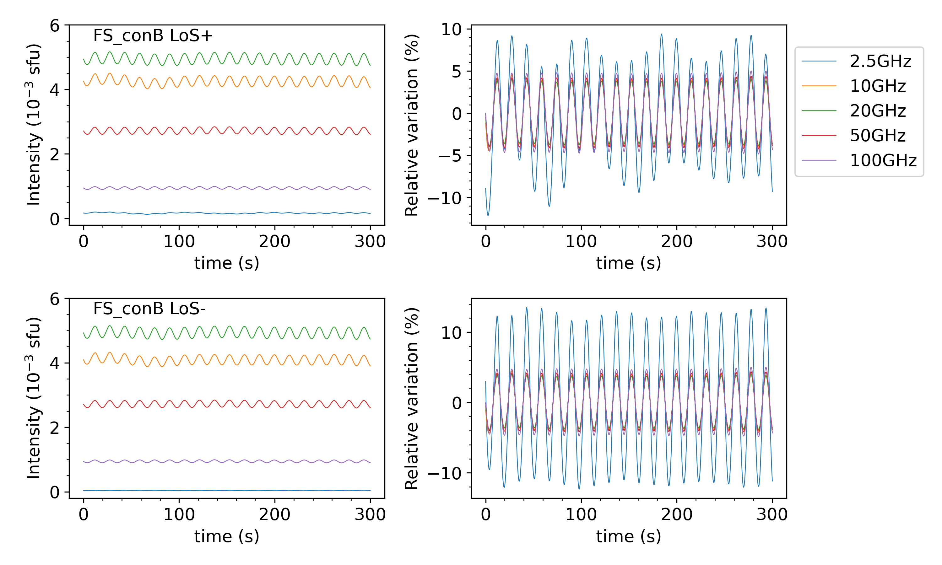
Figure 6: Similar to Figure 4 but for model FS_conB.

In model FS, the magnetic field strength is also fine-structured and the total magnetic flux is not the same as in model noFS. We conduct another MHD simulation, to be labeled ‘FS_conB’, where the equilibrium magnetic field has the same profile as in model noFS. Force balance in model FS_conB is maintained in a way that density structuring is counteracted by the temperature structuring. Figure 6 shows the emission intensities and their relative variations at five frequencies. Though the intensities are slightly different when compared with model FS, the relative variations are quite similar. Figure 7 compares the modulation amplitudes of model FS_conB and model FS. We find that the modulation amplitudes are different at some frequencies, whereas the general trend remains the same as model FS.

4.2 Number of the nonthermal electrons

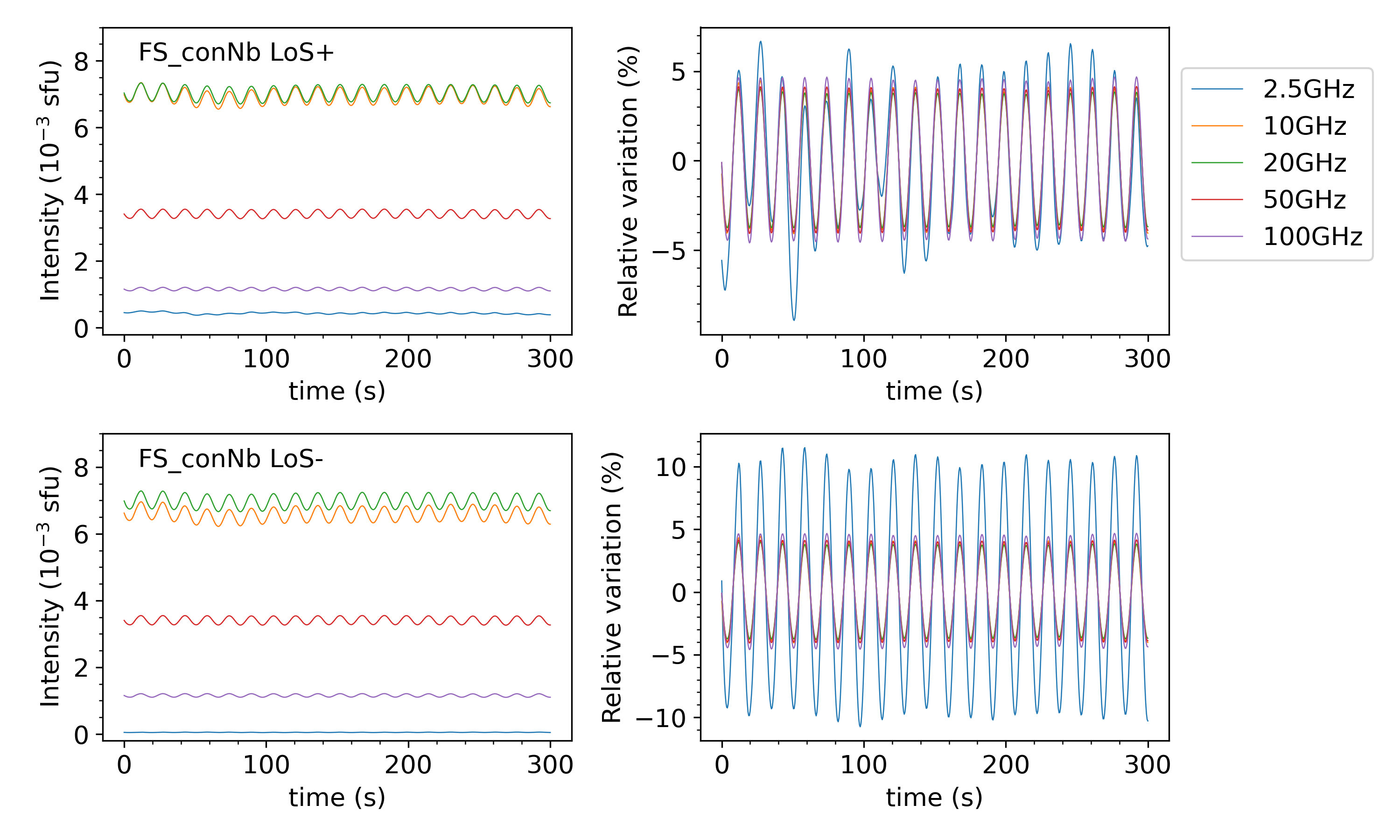
Figure 8: Similar to Figure 4 but for model FS_conNb.

When computing the GS emission, we assume that the number of the nonthermal electron is proportional to that of the thermal one, i.e., $N_{b}=0.005N_{e}$. The resultant number of the nonthermal electron inside the loop is 8.5% lower in model FS than in model noFS. To make sure that the total number of the nonthermal electron in model FS is exactly the same as in model noFS, we perform another forward modeling computation, to be labeled as ‘FS_conNb’, where $N_{b}=0.0055N_{e}$ is assumed. Figures 8 and 9 present the results of model FS_conNb. One sees that the intensity variations and the modulation amplitudes are quite similar to model FS.

4.3 Lower energy cut-off for nonthermal electrons

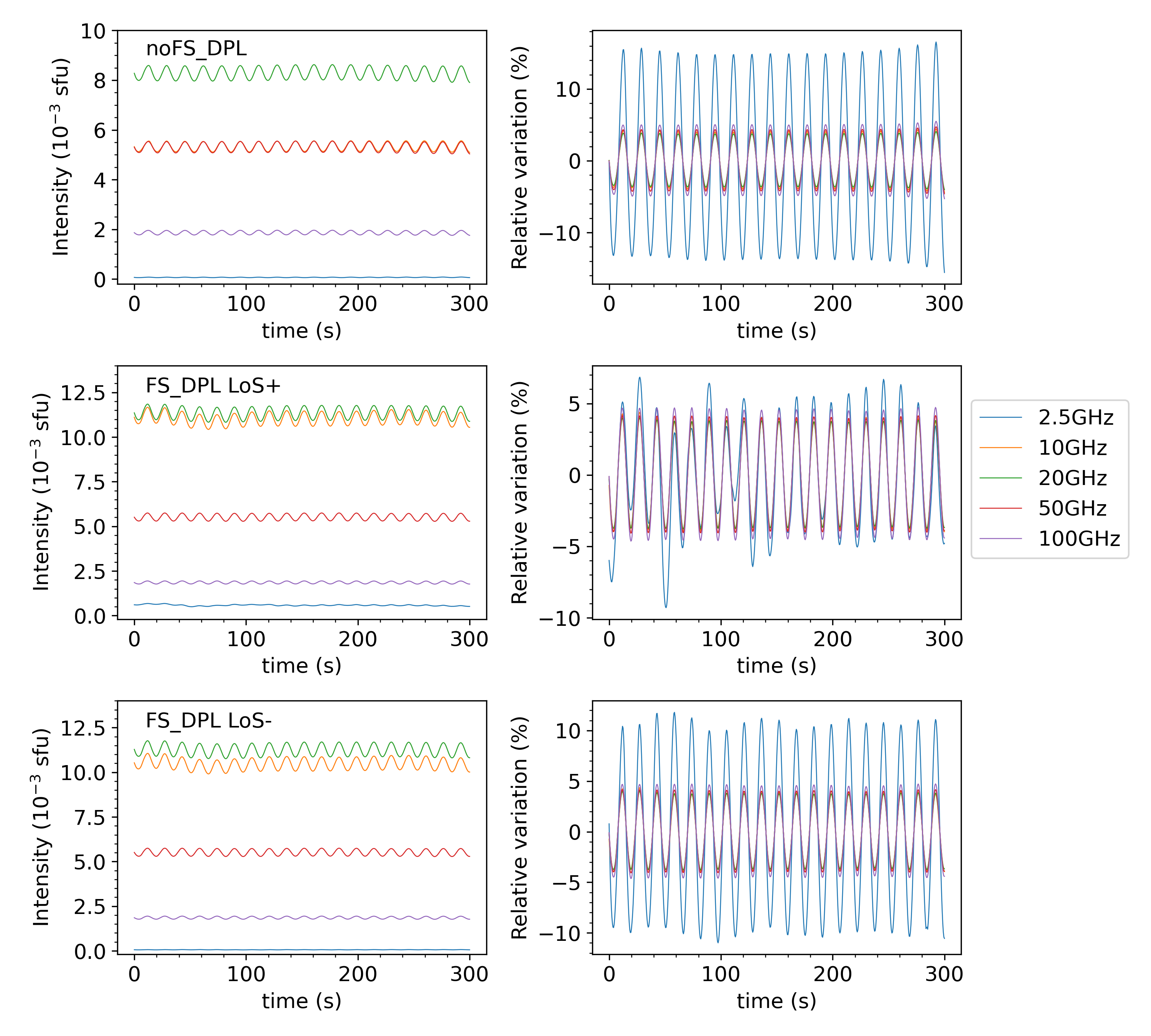
Figure 10: Similar to Figure 4 but for model noFS_DPL and FS_DPL.

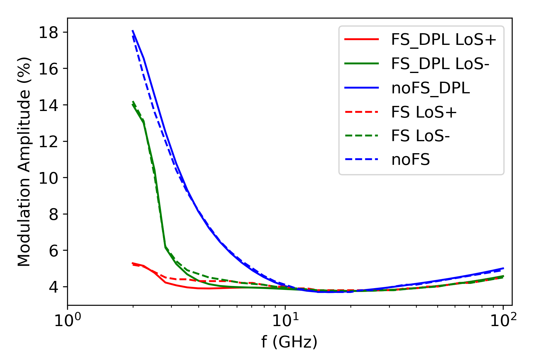
Figure 11: Modulation amplitudes for models with single power law (the dashed lines) and double power law (solid).

In the above mentioned forward modeling analysis, the lower energy cut-off of the nonthermal electrons is $E_{\rm min}=0.1$ MeV, which is higher than the typical value inferred from hard X-ray observations. The electrons with lower energies can influence the self-absorption at low frequencies, but their contribution to the GS emission is usually negligible (Holman, 2003). To address the influence of the lower energy nonthermal electrons in our model, we perform additional forward modeling analysis, to be labeled as noFS_DPL and FS_DPL. For these two models, the energy of the nonthermal electrons ranges from $E_{\rm min}=0.01$ MeV to $E_{\rm max}=10$ MeV. The spectrum of the nonthermal electrons takes a double power law shape with a break at $0.5$ MeV, with the spectral index being $\delta_{1}=1.5$ in the low energy band and $\delta_{2}=3.5$ in the high energy band, similar to Reznikova et al. (2014). Figure 10 shows the intensities and their variations. Relative to Figure 4, one finds that the intensities are somehow different while the relative variations are similar. Figure 11 compares the modulation amplitudes for models FS and noFS. We find that the influence of the lower energy nonthermal electrons is minor on the modulation amplitudes of the GS emission in our model.

5 Summary and Conclusion

Using three-dimensional MHD models, we study the influence of fine structures on the GS emission of flare loops modulated by axial fundamental sausage modes. The numerical models used for our reference computations are the same as those in G21, where two MHD models, namely noFS and FS, are simulated. Model noFS sees an equilibrium flare loop as a density-enhanced monolithic cylinder, whereas model FS modifies noFS by randomly introducing transverse fine structures to the loop interior. In both models, sausage modes are excited by an axisymmetric velocity perturbation. We compute GS emissions using the fast GS codes (Fleishman & Kuznetsov, 2010; Kuznetsov et al., 2011). We assume that the number density of the nonthermal electrons is proportional to that of the thermal electrons. The spectral index of the nonthermal electrons is 3.5, with its energy range being 0.1 MeV to 10 MeV. The pitch angle distribution is assumed to be isotropic. The temporal variation of the emission intensity is analyzed for a LoS crossing the loop center (red lines in Figure 1). We find that the low and high frequency intensities oscillate in-phase at the period of sausage mode for both model noFS and model FS. Fine structures only influence the intensity variation of the low-frequency emissions, dramatically reducing the modulation amplitudes. How significant this effect may be also depends on the orientation of the observer (i.e., LoS+ or LoS-). At high frequencies, the modulation amplitudes are not obviously influenced by the fine structures. Further computations (see Table 1) with different MHD models or nonthermal electron distributions are also examined, the results being largely similar to the reference computations. These results are helpful for understanding the GS emission modulated by sausage modes in flare loops, as well as for identifying sausage modes using radio observations. Combining our forward modeling results with the MHD simulations of G21, we conclude that the periodic oscillations of sausage modes are not wiped out by the loop fine structures, and sausage modes are a promising mechanism for interpreting flare QPPs even when flare loops are fine-structured.

Our results show that the modulation amplitudes of the GS emission intensities at low frequencies are dramatically reduced by the loop fine structures. This effect is mainly attributed to the optical thickness of the low-frequency emissions. However, such parameters as the total number of non-thermal electrons or the total magnetic flux can also influence the GS emissions and potentially affect the modulation amplitudes. The difference of the non-thermal electron numbers is 8.5% between model FS and model noFS. The influence of this difference on the modulation amplitudes is marginal, as shown in Figure 9. The influence of the total magnetic flux is slightly stronger. From Figure 7 one sees some difference between model FS and model FS_conB at low frequencies. Despite this difference, the modulation amplitudes of model FS_conB are still obviously smaller than those of model noFS. These results demonstrate that the optical thickness is the dominant factor for reducing the modulation amplitudes of the low-frequency emission intensities.

Even though the modulation amplitudes at low frequencies are significantly larger, the emission intensities at these frequencies are quite low, making their detections challenging. This is because the emission at low frequencies is significantly suppressed by the Razin effect. For flare loops with lower density, where the Razin suppression is not important, the intensity at low frequencies could be larger. In this case, the peak frequency is determined by self-absorption, so all frequencies below the peak should be optically thick. Our above mentioned effects relating to the optically thick regime are expected to be more pronounced and occur in a wider frequency range.

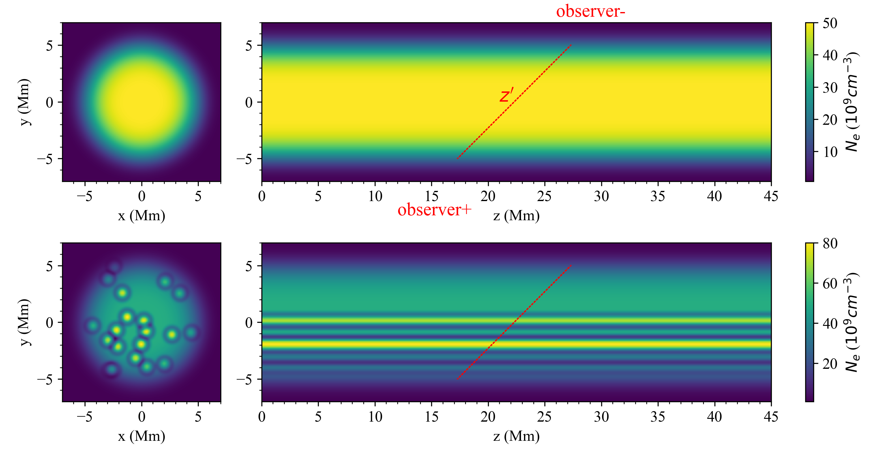
Figure 1: Distribution of the thermal electron number density ($N_{e}$) at $t=0$ for model noFS (top) and model FS (bottom) in the $x-y$ (left, with $z=0$) and $y-z$ (right, with $x=0$) planes. The red dotted lines mark the line of sight (LoS) projected onto the $y-z$ plane. Two LoS orientations are indicated by “observer+” (LoS+) and “observer-” (LoS-), respectively.

Figure 3: (a) The number density of nonthermal electrons ($N_{b}$), (b) the magnetic field strength ($B$), and (c) the Razin frequency ($f_{R}$) along the LoS. (d) The intensity profiles. (e) The optical depth averaged between the X and O modes. For model FS, the results for LoS+ and LoS- are discriminated by the solid and dash-dotted lines in (d) and (e).

Figure 4: Intensity (left) and its relative variation (right) at five frequencies for model noFS (top), model FS (LoS+, middle), and model FS (LoS-, bottom). The curves of relative variation are smoothed with a window of 2 periods.

Figure 7: Modulation amplitudes of model FS (the dashed lines) and model FS_conB (solid).

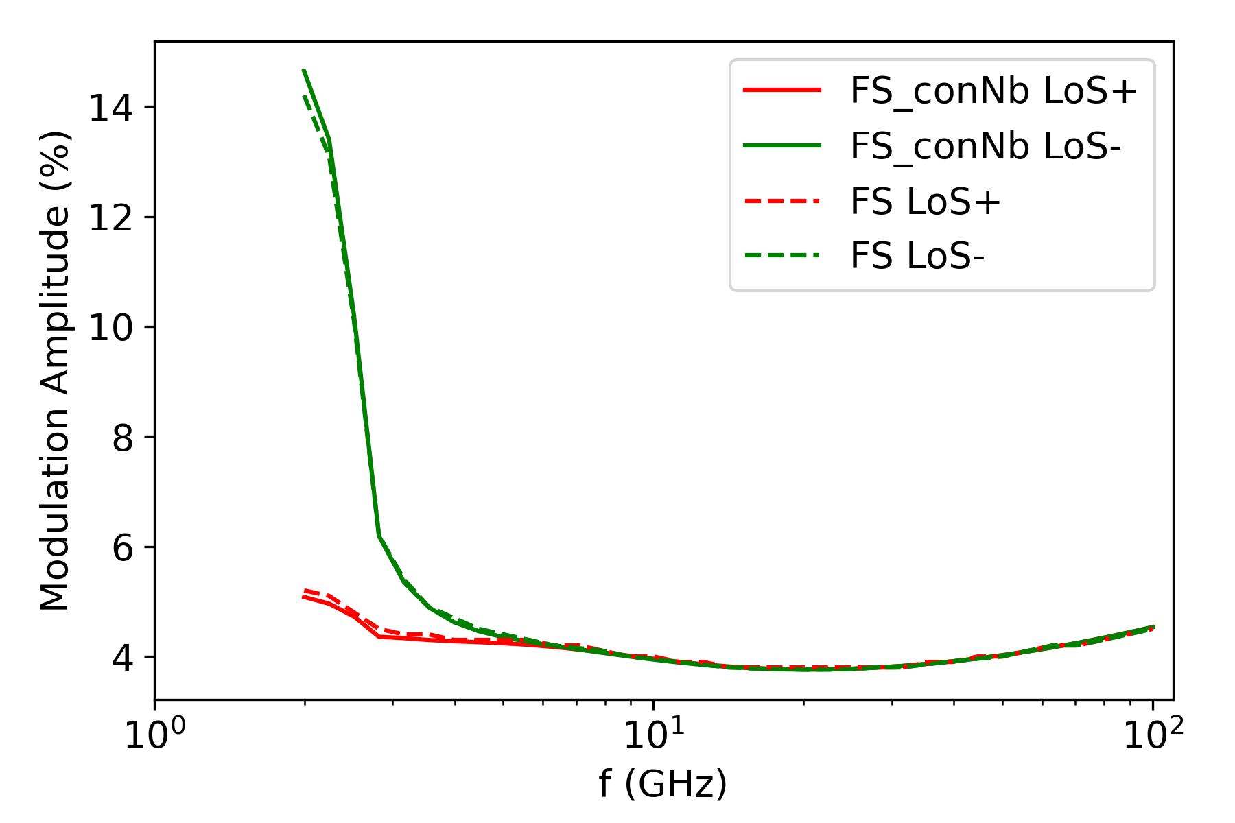
Figure 9: Modulation amplitudes of model FS (the dashed lines) and model FS_conNb (solid).

References

- Aschwanden & Peter (2017) Aschwanden, M. J., & Peter, H. 2017, ApJ, 840, 4
- Bastian et al. (1998) Bastian, T. S., Benz, A. O., & Gary, D. E. 1998, ARA&A, 36, 131
- Brooks et al. (2012) Brooks, D. H., Warren, H. P., & Ugarte-Urra, I. 2012, ApJ, 755, L33
- Cirtain et al. (2013) Cirtain, J. W., Golub, L., Winebarger, A. R., et al. 2013, Nature, 493, 501
- Dulk & Marsh (1982) Dulk, G. A., & Marsh, K. A. 1982, ApJ, 259, 350
- Edwin & Roberts (1983) Edwin, P. M., & Roberts, B. 1983, Sol. Phys., 88, 179
- Fleishman et al. (2008) Fleishman, G. D., Bastian, T. S., & Gary, D. E. 2008, ApJ, 684, 1433
- Fleishman & Kuznetsov (2010) Fleishman, G. D., & Kuznetsov, A. A. 2010, ApJ, 721, 1127
- Fleishman et al. (2022) Fleishman, G. D., Nita, G. M., Chen, B., Yu, S., & Gary, D. E. 2022, Nature, 606, 674
- Guarrasi et al. (2010) Guarrasi, M., Reale, F., & Peres, G. 2010, ApJ, 719, 576
- Guo et al. (2021) Guo, M., Li, B., & Shi, M. 2021, ApJ, 921, L17
- Guo et al. (2019) Guo, M., Van Doorsselaere, T., Karampelas, K., & Li, B. 2019, ApJ, 883, 20
- Holman (2003) Holman, G. D. 2003, ApJ, 586, 606. doi:10.1086/367554
- Kolotkov et al. (2015) Kolotkov, D. Y., Nakariakov, V. M., Kupriyanova, E. G., Ratcliffe, H., & Shibasaki, K. 2015, A&A, 574, A53
- Kupriyanova et al. (2020) Kupriyanova, E., Kolotkov, D., Nakariakov, V., et al. 2020, Solar-Terrestrial Physics, 6, 3
- Kuznetsov et al. (2011) Kuznetsov, A. A., Nita, G. M., & Fleishman, G. D. 2011, ApJ, 742, 87
- Kuznetsov et al. (2015) Kuznetsov, A. A., Van Doorsselaere, T., & Reznikova, V. E. 2015, Sol. Phys., 290, 1173
- Li et al. (2020) Li, B., Antolin, P., Guo, M. Z., et al. 2020, Space Sci. Rev., 216, 136
- Luna et al. (2008) Luna, M., Terradas, J., Oliver, R., & Ballester, J. L. 2008, ApJ, 676, 717
- Luna et al. (2010) —. 2010, ApJ, 716, 1371
- Magyar & Van Doorsselaere (2016) Magyar, N., & Van Doorsselaere, T. 2016, ApJ, 823, 82
- Melnikov et al. (2005) Melnikov, V. F., Reznikova, V. E., Shibasaki, K., & Nakariakov, V. M. 2005, A&A, 439, 727
- Mossessian & Fleishman (2012) Mossessian, G., & Fleishman, G. D. 2012, ApJ, 748, 140
- Nakariakov & Melnikov (2006) Nakariakov, V. M., & Melnikov, V. F. 2006, A&A, 446, 1151
- Nakariakov & Melnikov (2009) —. 2009, Space Sci. Rev., 149, 119
- Ofman (2009) Ofman, L. 2009, ApJ, 694, 502
- Pascoe et al. (2011) Pascoe, D. J., Wright, A. N., & De Moortel, I. 2011, ApJ, 731, 73
- Peter et al. (2013) Peter, H., Bingert, S., Klimchuk, J. A., et al. 2013, A&A, 556, A104
- Razin (1960) Razin, V. 1960, Izvestiya Vysshikh Uchebnykh Zavedenii. Radiofizika, 3, 584
- Reznikova et al. (2014) Reznikova, V. E., Antolin, P., & Van Doorsselaere, T. 2014, ApJ, 785, 86
- Reznikova et al. (2007) Reznikova, V. E., Melnikov, V. F., Su, Y., & Huang, G. 2007, Astronomy Reports, 51, 588
- Reznikova et al. (2015) Reznikova, V. E., Van Doorsselaere, T., & Kuznetsov, A. A. 2015, A&A, 575, A47
- Su et al. (2012) Su, J. T., Shen, Y. D., Liu, Y., Liu, Y., & Mao, X. J. 2012, ApJ, 755, 113
- Terradas et al. (2008) Terradas, J., Arregui, I., Oliver, R., et al. 2008, ApJ, 679, 1611
- Tian et al. (2016) Tian, H., Young, P. R., Reeves, K. K., et al. 2016, ApJ, 823, L16
- Tripathi et al. (2009) Tripathi, D., Mason, H. E., Dwivedi, B. N., del Zanna, G., & Young, P. R. 2009, ApJ, 694, 1256
- Van Doorsselaere et al. (2016) Van Doorsselaere, T., Kupriyanova, E. G., & Yuan, D. 2016, Sol. Phys., 291, 3143
- Van Doorsselaere et al. (2008) Van Doorsselaere, T., Ruderman, M. S., & Robertson, D. 2008, A&A, 485, 849
- Viall & Klimchuk (2012) Viall, N. M., & Klimchuk, J. A. 2012, ApJ, 753, 35
- Warren et al. (2003) Warren, H. P., Winebarger, A. R., & Mariska, J. T. 2003, ApJ, 593, 1174
- Wedemeyer et al. (2016) Wedemeyer, S., Bastian, T., Brajša, R., et al. 2016, Space Sci. Rev., 200, 1
- Zimovets et al. (2013) Zimovets, I. V., Kuznetsov, S. A., & Struminsky, A. B. 2013, Astronomy Letters, 39, 267
- Zimovets & Struminsky (2010) Zimovets, I. V., & Struminsky, A. B. 2010, Sol. Phys., 263, 163
- Zimovets et al. (2021) Zimovets, I. V., McLaughlin, J. A., Srivastava, A. K., et al. 2021, Space Sci. Rev., 217, 66