Locally weighted minimum contrast estimation for spatio-temporal log-Gaussian Cox processes

Abstract

We propose a local version of spatio-temporal log-Gaussian Cox processes using Local Indicators of Spatio-Temporal Association (LISTA) functions into the minimum contrast procedure to obtain space as well as time-varying parameters. We resort to the joint minimum contrast fitting method to estimate the set of second-order parameters. This approach has the advantage of being suitable in both separable and non-separable parametric specifications of the correlation function of the underlying Gaussian Random Field. We present simulation studies to assess the performance of the proposed fitting procedure, and show an application to seismic spatio-temporal point pattern data.

1 Introduction

Interest in methods for analysing spatial and spatio-temporal point processes is increasing across many fields of science, notably in ecology, epidemiology, geoscience, astronomy, econometrics, and crime research (Baddeley et al.,, 2015; Diggle,, 2013). When the structure of a given point pattern is observed, it is assumed to come from a realisation of an underlying generating process, whose properties are estimated and then used to describe the structure of the observed pattern. The first step in analysing a point pattern is to learn about its first-order characteristics, studying the relationship of the points with the underlying environmental variables that describe the observed heterogeneity. When the purpose of the analysis is to describe the possible interaction among points, that is, if the given data exhibit spatial inhibition or aggregation, the second-order properties of the process are analysed. However, in the analysis of spatial (and spatio-temporal) point process data it can be difficult to disentangle the two previous aspects, i.e. the heterogeneity corresponding to spatial variation of the intensity and the dependence structure amongst the points (Illian et al.,, 2008; Diggle,, 2013). For this reason, it is attractive and motivating to define and estimate models that account simultaneously for the dependence structure among events, including also the effect of the observed covariates.

Cox processes are a class of models for point phenomena that are environmentally driven and have a clustered structure. They are Poisson processes with a random intensity function depending on unobservable external factors. Two notable classes of Cox point processes are the shot-noise Cox processes (Møller,, 2003) and the log-Gaussian Cox processes (LGCPs) (Møller et al.,, 1998).

LGCPs are arguably the most prominent clustering models, for their flexibility and relatively tractability for describing spatial and spatio-temporal correlated phenomena specifying the moments of an underlying Gaussian Random Field (GRF). Therefore, the main interest is in the estimation of the first and second-order characteristics of the process that depend on the moments of the GRF.

In both purely spatial and spatio-temporal studies, the choice of the estimation procedure depends on several aspects that relate to the application context, the goals of the analysis, and the required computational time. Diggle et al., (2013) discusses the three main estimation methods (moment-based, maximum likelihood and Bayesian estimation) for LGCPs. Siino et al., 2018a describe earthquake sequences comparing several Cox model specifications (with separable and non-separable spatio-temporal covariance functions) estimating parameters through the minimum contrast method.

The aforementioned models can be referred to as ‘global’ models, as they are globally defined and the process properties and estimated parameters are assumed to be constant all through the study area. However, a model with constant parameters, may not adequately represent detailed local variations in the data, since the pattern may present spatial and temporal variations due to the influence of covariates, the scale or spacing between points, and also perhaps due to the abundance of points. Indeed, a different way of analysing a point pattern can be based on local techniques identifying specific and undiscovered local structure, for instance sub-regions characterised by different interactions among points, intensity and influence of covariates.

On one hand, local second-order statistics have been used to obtain further insight into the local structure of the analysed point pattern. While the use of global spatio-temporal second-order summary statistics is a well-established practice to describe global interaction structures between points in a point pattern (Ripley,, 1977; Illian et al.,, 2008; Gabriel and Diggle,, 2009), the use of local tools was firstly advocated by Siino et al., 2018b , introducing the Local Indicators of Spatio-Temporal Association (LISTA) functions as an extension of the purely spatial Local Indicators, whose definition was given by Anselin, (1995). Successively, Adelfio et al., (2020) introduced local versions of both the homogeneous and inhomogeneous spatio-temporal $K$-functions, and used them as diagnostic tools, while also retaining for local information, showing that the local inhomogeneous $K$-functions can be helpful to assess the goodness-of-fit of different spatio-temporal models, with the advantage of not relying on any particular model assumption on the data.

On the other hand, the literature about local models for point processes is quite rare. For spatial point processes, Baddeley, (2017) presents a general framework based on the local composite likelihood to detect and model gradual spatial variation in any parameter of a spatial stochastic model (such as Poisson, Gibbs and Cox processes). In particular, the parameters in the model that govern the intensity, the dependence of the intensity on the covariates and the spatial interaction between points, are estimated locally. Moreover, this approach has the advantage to detect and model spatial variation in any property of a point process, within a formal likelihood framework providing space-varying parameter estimates, confidence intervals and hypothesis tests.

D’Angelo et al., 2022b showed that Baddeley,’s purely local models provide good inferential results by applying them to earthquake data. However, that work did not account for the temporal dimension of the seismic events, whose realisations depend on their past history, as proved by the existence of aftershocks. Motivated by this, we propose a local version of spatio-temporal LGCPs employing LISTA functions plugged into the minimum contrast procedure to obtain space as well as time-varying parameters. For the parameters of the deterministic part, we follow Baddeley and Turner, (2000), using a quadrature scheme for the locally weighted log-linear Poisson regression. For the parameters of the coviariance structure, we resort to the joint minimum contrast fitting method proposed by Siino et al., 2018a to estimate the set of second-order parameters of the spatio-temporal LGCPs. This approach has the advantage of being suitable in both separable and non-separable parametric specifications of the correlation function of the underlying GRF.

We therefore introduce the local estimation, obtaining a whole set of parameters for each point of the analysed dataset, and we refer to this new procedure as locally weighted spatio-temporal minimum contrast. We show some simulations, finding promising results as the estimates tend to be quite precise on average if compared to the ’global’ counterpart, while also reflecting the assumed variability in space and time. To enforce these results, we apply the proposed methodology to a real dataset in seismicity, considering the quite convenient separable covariance function of the LGCP. All the codes are written in the software R Core Team, (2020) language, and are available from the first author.

The structure of the paper is as follows. Section 2 is devoted to the introduction of basic definitions of spatio-temporal point processes. Section 3 briefly reviews the class of spatio-temporal LGCPs. In Section 4, the proposed local minimum contrast estimation based on the LISTA functions is presented. Section 5 reports the diagnostic procedure used to assess the goodness-of-fit of a global LGCP, and a proposed modification to deal with local LGCPs. Then, the performance of the proposed local estimation method is assessed in Section 6 through a simulation study. An application to real seismic data comes in Section 7. Finally, the paper ends with some conclusions in Section 8.

2 Spatio-temporal point processes and main characteristics

We consider a spatio-temporal point process with no multiple points as a random countable subset $X$ of $\mathbb{R}^{2}\times\mathbb{R}$, where a point $(\textbf{u},t)\in X$ corresponds to an event at $\textbf{u}\in\mathbb{R}^{2}$ occurring at time $t\in\mathbb{R}$. A typical realisation of a spatio-temporal point process $X$ on $\mathbb{R}^{2}\times\mathbb{R}$ is a finite set $\{(\textbf{u}_{i},t_{i})\}^{n}_{i=1}$ of distinct points within a bounded spatio-temporal region $W\times T\subset\mathbb{R}^{2}\times\mathbb{R}$, with area $|W|>0$ and length $|T|>0$, where $n\geq 0$ is not fixed in advance. In this context, $N(A\times B)$ denotes the number of points of a set $(A\times B)\cap X$, where $A\subseteq W$ and $B\subseteq T$. As usual (Daley and Vere-Jones,, 2007), when $N(W\times T)<\infty$ with probability 1, which holds e.g. if $X$ is defined on a bounded set, we call $X$ a finite spatio-temporal point process.

For a given event $(\textbf{u},t)$, the events that are close to $(\textbf{u},t)$ in both space and time, for each spatial distance $r$ and time lag $h$, are given by the corresponding spatio-temporal cylindrical neighbourhood of the event $(\textbf{u},t)$, which can be expressed by the Cartesian product as

$$b((\textbf{u},t),r,h)=\{(\textbf{v},s):||\textbf{u}-\textbf{v}||\leq r,|t-s|\leq h\},\quad\quad(\textbf{u},t),(\textbf{v},s)\in W\times T,$$

where $||\cdot||$ denotes the Euclidean distance in $\mathbb{R}^{2}$. Note that $b((\textbf{u},t),r,h)$ is a cylinder with centre (u, t), radius $r$, and height $2h$.

Product densities $\lambda^{(k)},k\in\mathbb{N}\text{ and }k\geq 1$, arguably the main tools in the statistical analysis of point processes, may be defined through the so-called Campbell Theorem (see Daley and Vere-Jones, (2007)), which states that given a spatio-temporal point process $X$, and for any non-negative function $f$ on $(\mathbb{R}^{2}\times\mathbb{R})^{k}$, we have

$$\mathbb{E}\Bigg{[}\sum_{\zeta_{1},\dots,\zeta_{k}\in X}^{\neq}f(\zeta_{1},\dots,\zeta_{k})\Bigg{]}=\int_{\mathbb{R}^{2}\times\mathbb{R}}\dots\int_{\mathbb{R}^{2}\times\mathbb{R}}f(\zeta_{1},\dots,\zeta_{k})\lambda^{(k)}(\zeta_{1},\dots,\zeta_{k})\prod_{i=1}^{k}\text{d}\zeta_{i},$$

that constitutes an essential result in spatio-temporal point process theory. In particular, for $k=1$ and $k=2$, these functions are respectively called the (first-order) intensity function $\lambda$ and the (second-order) product density $\lambda^{(2)}$. Broadly speaking, the intensity function describes the rate at which the events occur in the given spatio-temporal region, while the second-order product densities are used when the interest is in describing spatio-temporal variability and correlations between pair of points of a pattern. They represent the point process analogues of the mean function and the covariance function of a real-valued process, respectively. Then, the intensity function is defined as

$$\lambda(\textbf{u},t)=\lim_{|\text{d}\textbf{u}\times\text{d}t|\rightarrow 0}\frac{\mathbb{E}[N(\text{d}\textbf{u}\times\text{d}t)]}{|\text{d}\textbf{u}\times\text{d}t|},$$

where $\text{d}\textbf{u}\times\text{d}t$ defines a small region around the point $(\textbf{u},t)$ and $|\text{d}\textbf{u}\times\text{d}t|$ is its volume. The second-order intensity function is

$$\lambda^{(2)}((\textbf{u},t),(\textbf{v},s))=\lim_{|\text{d}\textbf{u}\times\text{d}t|,|\text{d}\textbf{v}\times\text{d}s|\rightarrow 0}\frac{\mathbb{E}[N(\text{d}\textbf{u}\times\text{d}t)N(\text{d}\textbf{v}\times\text{d}s)]}{|\text{d}\textbf{u}\times\text{d}t||\text{d}\textbf{v}\times\text{d}s|}.$$

Finally, the pair correlation function

$$g((\textbf{u},t),(\textbf{v},s))=\frac{\lambda^{(2)}((\textbf{u},t),(\textbf{v},s))}{\lambda(\textbf{u},t)\lambda(\textbf{v},s)}$$

can be interpreted formally as the standardised probability density that an event occurs in each of two small volumes, $\text{d}\textbf{u}\times\text{d}t$ and $\text{d}\textbf{v}\times\text{d}s$, in the sense that for a Poisson process, $g((\textbf{u},t),(\textbf{v},s))=1$.

3 Spatio-temporal log-Gaussian Cox processes

In the Euclidean context, LGCPs are one of the most prominent clustering models. By specifying the intensity of the process and the moments of the underlying GRF, it is possible to estimate both the first and second-order characteristics of the process. Following the inhomogeneous specification in Diggle et al., (2013), a LGCP for a generic point in space and time has the intensity

$$\Lambda(\textbf{u},t)=\lambda(\textbf{u},t)\exp(S(\textbf{u},t))$$

where $S$ is a Gaussian process with $\mathbb{E}(S(\textbf{u},t))=\mu=-0.5\sigma^{2}$ and so $\mathbb{E}(\exp{S(\textbf{u},t)})=1$ and with variance and covariance matrix $\mathbb{C}(S(\textbf{u}_{i},t_{i}),S(\textbf{u}_{j},t_{j}))=\sigma^{2}\gamma(r,h)$ under the stationary assumption, with $\gamma(\cdot)$ the correlation function of the GRF, and $r$ and $h$ some spatial and temporal distances. Following Møller et al., (1998), the first-order product density and the pair correlation function of an LGCP are $\mathbb{E}(\Lambda(\textbf{u},t))=\lambda(\textbf{u},t)$ and $g(r,h)=\exp(\sigma^{2}\gamma(r,h))$, respectively. In this paper, we first consider a separable structure for the covariance function of the GRF (Brix and Diggle,, 2001) that has exponential form for both the spatial and the temporal components,

$$\mathbb{C}(r,h)=\sigma^{2}\exp\bigg{(}\frac{-r}{\alpha}\bigg{)}\exp\bigg{(}\frac{-h}{\beta}\bigg{)},$$ (1)

where $\sigma^{2}$ is the variance, $\alpha$ is the scale parameter for the spatial distance and $\beta$ is the scale parameter for the temporal one. The exponential form is widely used in this context and nicely reflects the decaying correlation structure with distance or time. Moreover, we may consider a non-separable covariance of the GRF useful to describe more general situations. Gneiting et al., (2006) review parametric non-separable space-time covariance functions for geostatistical models. Following the parametrisation in Schlather et al., (2015), Gneiting covariance function can be written as

$$\mathbb{C}(r,h)=(\psi(h)+1)^{-d/2}\varphi\bigg{(}\frac{r}{\sqrt{\psi(h)+1}}\bigg{)}\qquad r\geq 0,\quad h\geq 0,$$

where $\varphi(\cdot)$ is a complete monotone function associated to the spatial structure, and $\psi(\cdot)$ is a positive function with a completely monotone derivative associated to the temporal structure of the data. For example, the choice $d=2$, $\varphi(r)=\sigma^{2}\exp(-(\frac{r}{\alpha})^{\gamma_{s}})$ and $\psi(h)=((\frac{h}{\beta})^{\gamma_{t}}+1)^{\delta/\gamma_{t}}$ yields to the parametric family

$$\mathbb{C}(r,h)=\frac{\sigma^{2}}{((\frac{h}{\beta})^{\gamma_{t}}+1)^{\delta/\gamma_{t}}}\exp\Biggl{(}-\frac{(\frac{r}{\alpha})^{\gamma_{s}}}{((\frac{h}{\beta})^{\gamma_{t}}+1)^{\delta/(2\gamma_{t})}}\Biggl{)},$$ (2)

where $\alpha>0$ and $\beta>0$ are scale parameters of space and time, $\delta$ takes values in $(0,2]$, and $\sigma^{2}$ is the variance. Another parametric covariance belongs to the Iaco-Cesare family (De Cesare et al.,, 2002; De Iaco et al.,, 2002), and there is a wealth of covariance families that could well be used for our purposes.

4 Model estimation

Driven by a GRF, controlled in turn by a specified covariance structure, the implementation of the LGCP framework in practice requires a proper estimate of the intensity function. In general, the Cox model is estimated by a two-step procedure, involving first the intensity and then the cluster or correlation parameters. First, a Poisson process with a particular model for the log-intensity is fitted to the point pattern data, providing the estimates of the coefficients of all the terms that characterise the intensity. Then, the estimated intensity is taken as the true one and the cluster or correlation parameters are estimated using either the method of minimum contrast (Pfanzagl,, 1969; Eguchi,, 1983; Diggle,, 1979; Diggle and Gratton,, 1984; Møller et al.,, 1998; Davies and Hazelton,, 2013; Siino et al., 2018a, ), Palm likelihood (Ogata and Katsura,, 1991; Tanaka et al.,, 2008), or composite likelihood (Guan,, 2006). The most common technique is the minimum contrast, and it is the method which we shall refer to here.

In the following, we first review and extend the statistical theory and computational strategies for local estimation and inference for spatio-temporal Poisson point processes, in Section 4.1. Then, in Section 4.2 we recall the joint minimum contrast procedure, that we extend in Section 4.3 to the local context.

4.1 Estimating the first-order intensity function through local likelihood

We assume that the template model is a Poisson process, with a parametric intensity or rate function

$$\lambda(\textbf{u},t;\theta),\quad X\in W,\quad t\in T,\quad\theta\in\Theta.$$

The log-likelihood is

$$\log L(\theta)=\sum_{i}\lambda(\textbf{u}_{i},t_{i};\theta)-\int_{W}\int_{T}\lambda(\textbf{u},t;\theta)\text{d}t\text{d}u$$ (3)

up to an additive constant, where the sum is over all points $\textbf{u}_{i}$ in $X$. We often consider intensity models of log-linear form

$$\lambda(\textbf{u},t;\theta)=\exp(\theta Z(\textbf{u},t)+B(\textbf{u},t)),\quad\textbf{u}\in W,\quad t\in T$$ (4)

where $Z(\textbf{u},t)$ is a vector-valued covariate function, and $B(\textbf{u},t)$ is a scalar offset.

4.1.1 Quadrature scheme

Following Berman and Turner, (1992), we use a finite quadrature approximation to the log-likelihood, as implemented in the spatstat package (Baddeley and Turner,, 2005). Renaming the data points as $\textbf{x}_{1},\dots,\textbf{x}_{n}$ with $(\textbf{u}_{i},t_{i})=\textbf{x}_{i}$ for $i=1,\dots,n$, then generate $m$ additional “dummy points” $(\textbf{u}_{n+1},t_{n+1})\dots,(\textbf{u}_{m+n},t_{m+n})$ to form a set of $n+m$ quadrature points (where $m>n$). Then we determine quadrature weights $a_{1},\dots,a_{m}$ so that integrals in (3) can be approximated by a Riemann sum

$$\int_{W}\int_{T}\lambda(\textbf{u},t;\theta)\text{d}t\text{d}u\approx\sum_{k=1}^{n+m}a_{k}\lambda(\textbf{u},t;\theta)$$ (5)

where $a_{k}$ are the quadrature weights such that $\sum_{k=1}^{n+m}a_{k}=l(W\times T)$ where $l$ is the Lebesgue measure.

Then the log-likelihood (3) of the template model can be approximated by

$$\log L(\theta)\approx\sum_{i}\log\lambda(\textbf{x}_{i};\theta)+\sum_{j}(1-\lambda(\textbf{u}_{j},t_{j};\theta))a_{j}=\sum_{j}e_{j}\log\lambda(\textbf{u}_{j},t_{j};\theta)+(1-\lambda(\textbf{u}_{j},t_{j};\theta))a_{j}$$

where $e_{j}=1\{j\leq n\}$ is the indicator that equals $1$ if $u_{j}$ is a data point. Writing $y_{j}=e_{j}/a_{j}$ this becomes

$$\log L(\theta)\approx\sum_{j}a_{j}(y_{j}\log\lambda(\textbf{u}_{j},t_{j};\theta)-\lambda(\textbf{u}_{j},t_{j};\theta))+\sum_{j}a_{j}.$$ (6)

Apart from the constant $\sum_{j}a_{j}$, this expression is formally equivalent to the weighted log-likelihood of a Poisson regression model with responses $y_{j}$ and means $\lambda(\textbf{u}_{j},t_{j};\theta)=\exp(\theta Z(\textbf{u}_{j},t_{j})+B(\textbf{u}_{j},t_{j}))$. This can be maximised using standard GLM software. For more details see Berman and Turner, (1992); Baddeley et al., (2000, 2005) Section 9.8.

We define the spatio-temporal quadrature scheme by defying a spatio-temporal partition of $W\times T$ into cubes $C_{k}$ of equal volume $\nu$, assigning the weight $a_{k}=\nu/n_{k}$ to each quadrature point (dummy or data) where $n_{k}$ is the number of points that lie in the same cube as the point $u_{k}$ (Raeisi et al.,, 2021).

The number of dummy points should be sufficient for an accurate estimate of the likelihood. Following Baddeley et al., (2000) and Raeisi et al., (2021), we start with a number of dummy points $m\approx 4n$, increasing it until $\sum_{k}a_{k}=l(W\times T)$.

4.1.2 Local Poisson models in space and time

The local log-likelihood associated with the spatio-temporal location $(\textbf{v},s)$ is given by

$$\log L((\textbf{v},s);\theta)=\sum_{i}w_{\sigma_{s}}(\textbf{u}_{i}-\textbf{v})w_{\sigma_{t}}(t_{i}-s)\lambda(\textbf{u}_{i},t_{i};\theta)-\int_{W}\int_{T}\lambda(\textbf{u},t;\theta)w_{\sigma_{s}}(\textbf{u}_{i}-\textbf{v})w_{\sigma_{t}}(t_{i}-s)\text{d}t\text{d}u$$ (7)

where $w_{\sigma_{s}}$ and $w_{\sigma_{t}}$ are weight functions, and $\sigma_{s},\sigma_{t}>0$ are the smoothing bandwidths. It is not necessary to assume that $w_{\sigma_{s}}$ and $w_{\sigma_{t}}$ are probability densities. For simplicity, we shall consider only kernels of fixed bandwidth, even though spatially adaptive kernels could also be used. Note that if the template model is the homogeneous Poisson process with intensity $\lambda$, then the local likelihood estimate $\hat{\lambda}(\textbf{v},s)$ reduces to the kernel estimator of the point process intensity (Diggle,, 2013) with kernel proportional to $w_{\sigma_{s}}w_{\sigma_{t}}$.

We now use in (7) a similar approximation as in (6) for the local log-likelihood associated with each desired location $(\textbf{v},s)\in W\times T$

$$\log L((\textbf{v},s);\theta)\approx\sum_{j}w_{j}(\textbf{v},s)a_{j}(y_{j}\log\lambda(\textbf{u}_{j},t_{j};\theta)-\lambda(\textbf{u}_{j},t_{j};\theta))+\sum_{j}w_{j}(\textbf{v},s)a_{j},$$ (8)

where $w_{j}(\textbf{v},s)=w_{\sigma_{s}}(\textbf{v}-\textbf{u}_{j})w_{\sigma_{t}}(s-t_{j})$.

Basically, for each desired location $(\textbf{v},s)$, we replace the vector of quadrature weights $a_{j}$ by $a_{j}(\textbf{v},s)=w_{j}(\textbf{v},s)a_{j}$ where $w_{j}(\textbf{v},s)=w_{\sigma_{s}}(\textbf{v}-\textbf{u}_{j})w_{\sigma_{t}}(s-t_{j})$, and use the GLM software to fit the Poisson regression. The local likelihood is defined at any location $(\textbf{v},s)$ in continuous space. In practice it will be enough to consider a grid of points $(\textbf{v},s)$. The choice of the grid depends on the computing resources, the computations required at each location, and the spatial resolution required.

Choice of the bandwidths

Bandwidth selection is always an unavoidable topic with kernel estimation. In principle, the bandwidth should be selected according to data resolution, which is at the order of 1-10 times of the nearest neighbouring distance (Zhuang,, 2020). However, the simple kernel estimate with a fixed bandwidth has a serious disadvantage, that is, for a (spatially) clustered point dataset, a small bandwidth gives a noisy estimate for the sparsely populated area, whereas a large bandwidth mixes up the boundaries between the densely populated and sparsely populated areas. Therefore, instead of the kernel estimates $w$ with fixed bandwidth $\sigma$, we can adopt variable kernel estimates where $\sigma_{j}$ represents the varying bandwidth calculated for each event $j$. We can determine the variable bandwidth by

$$\sigma_{j}=max\{\epsilon,\inf(r:N[B(\textbf{u}_{j};r)]>n_{p})\},$$

where $\epsilon$ is a small number, $B(\textbf{u}_{j};r)$ is the disk centered at $\textbf{u}_{j}$ with a radius of $r$, and $n_{p}$ is a positive integer, i.e. $\sigma_{j}$ is the distance to $n_{p}$-th closest event. In other words, once a suitable integer between 10 and 100 for the parameter $n_{p}$ is chosen, we calculate a bandwidth value $\sigma_{j}$, of each event $j$, as the radius of the smallest circle centered at the location of the $j$th event that includes at least $n_{p}$ other events. See Silverman, (1986) for similar locally dependent estimates, Zhuang et al., (2002) for their use in a seismic context, and Musmeci and Vere-Jones, (1986); Choi and Hall, (1999) for similar ideas.

4.2 Estimating the covariance parameters through minimum contrast

The arbitrariness of the minimum contrast procedure can be criticised, however the relative computational simplicity with respect to other estimation procedures (such as likelihood or Bayesian estimation procedures) makes this method suitable for estimating Cox process parameters (Siino et al., 2018a, ). The procedure selects those parameters that minimise the squared discrepancy between parametric and non-parametric representations of the second-order properties of the LGCP. Minimum contrast estimation is used because direct likelihood-based inference for the parameters of interest is generally not possible. It is important to notice that the intuitiveness of the minimum contrast procedure is offset by the numerous subjective decisions that must be made in order to implement the criterion in practice.

Let the function $J$ represent either the pair correlation function $g$ or the $K$-function, and $\hat{J}$ stands for the corresponding non-parametric estimate. The minimum contrast estimates $\hat{\sigma}^{2}$ and $\hat{\alpha}$ are found minimising

$$M_{J}\{\sigma^{2},\alpha\}=\int_{r_{0}}^{r_{max}}\phi(r)\{\nu[\hat{J}(r)]-\nu[J(r;\sigma^{2},\alpha)]\}^{2}\text{d}r$$ (9)

where $r_{0}$ and $r_{max}$ are the lower and upper lag limits of the contrast criterion, $\phi$ denotes some scalar weight associated with each spatial lag $r$, $\nu$ represents some transformation of its argument and the approximation of $M_{J}$ is obtained by summing over a fine sequence of lags $R=\{r_{0},r_{1},\dots,r_{max}\}$ equally spaced, so that $R_{diff}=r_{b}-r_{a},b>a$

$$M_{J}\{\sigma^{2},\alpha\}\approx R_{diff}^{-1}\sum_{r\in R}\phi(r)\{\nu[\hat{J}(r)]-\nu[J(r;\sigma^{2},\alpha)]\}^{2}.$$

Estimation of $\tau$ is performed minimising the squared discrepancy between the covariance function between the expected frequency of observations at two points in time $C(t,t-h;\tau)$ and its natural estimator, the empirical autocovariance function $\hat{C}(t,t-h)$, for a finite sequence of temporal lags. The contrast criterion for the temporal part is

$$M_{C}\{\tau\}=\sum_{h=1}^{h_{max}}\sum_{t=h+1}^{T}[\hat{C}(t,t-h)-C(t,t-h;\tau)]^{2},$$ (10)

for some user-specified value of $h_{max}<T$, that it is the temporal counterpart of $r_{max}$. The theoretical version of the temporal covariance depends upon the spatial parameters; thus the spatial parameters must be estimated first and then plugged into the temporal minimum contrast procedure.

Alternatively, Siino et al., 2018a proposed a new fitting method to estimate the set of second-order parameters for the class of LGCPs with constant first-order intensity function. Hereafter we will denote by $\boldsymbol{\theta}$ the vector of (first-order) intensity parameters, and by $\boldsymbol{\psi}$ the cluster parameters, also denoted as correlation or interaction parameters by some authors. For instance, in the case of a spatio-temporal LGCP with exponential covariance, as the one in Equation (1), the cluster parameters correspond to $\boldsymbol{\psi}=(\sigma,\alpha,\beta)$. The second-order parameters $\boldsymbol{\psi}$ are found by minimising

$$M_{J}\{\boldsymbol{\psi}\}=\int_{h_{0}}^{h_{max}}\int_{r_{0}}^{r_{max}}\phi(r,h)\{\nu[\hat{J}(r,h)]-\nu[J(r,h;\boldsymbol{\psi})]\}^{2}\text{d}r\text{d}h,$$ (11)

where $\phi(r,h)$ is a weight that depends on the space-time distance and $\nu$ is a transformation function. With simulations, Siino et al., 2018a show that the joint minimum contrast procedure, based on the spatio-temporal pair correlation function, provides reliable estimates. Its main advantage is that it can be used in the case of both separable and non-separable parametric specifications of the correlation function of the underlying GRF. Therefore, it represents a more flexible method with respect to other current available methods, and it is the method that we chose to extend into the local context.

4.3 Locally weighted spatio-temporal minimum contrast

In the purely spatial context, a localised version of minimum contrast is developed using the local $K$-functions or local pair correlation functions by Baddeley, (2017), bearing a very close resemblance to the local Palm likelihood approach, whose implementation is provided by the function locmincon() of the R package spatstat.local (Baddeley,, 2019).

Combining the joint minimum contrast (Siino et al., 2018a, ) and the local minimum contrast (Baddeley,, 2017) procedures, we can obtain a vector of parameters $\boldsymbol{\psi}_{i}$ for each point $i$, by minimising

$$M_{J,i}\{\boldsymbol{\psi}_{i}\}=\int_{h_{0}}^{h_{max}}\int_{r_{0}}^{r_{max}}\phi(r,h)\{\nu[\bar{J}_{i}(r,h)]-\nu[J(r,h;\boldsymbol{\psi})]\}^{2}\text{d}r\text{d}h,$$ (12)

where $\bar{J}_{i}(r,h)$ is the average of the local functions $\hat{J}_{i}(r,h)$, weighted by some point-wise kernel estimates. This procedure not only provides individual estimates, but it does also account for the vicinity of the observed points, and therefore the contribution of their displacement on the estimation procedure. This conceptually resembles the methodology used for the local log-likelihood in Section (4.1.2). Following Siino et al., 2018a , we suggest using $\phi(r,h)=1$ and $\nu$ as the identity function. Then, $r_{max}$ and $h_{max}$ are selected as 1/4 of the maximum observable spatial and temporal distances.

Thus, consider again the weights $w_{i}=w_{i,\sigma_{s}}w_{i,\sigma_{t}}$ given by some kernel estimates. The same considerations hold for the choice of the bandwidth in the local log-likelihood. Then, the averaged weighted local statistics $\bar{J}_{i}(r,h)$ in (12), for each point $i$, is

$$\bar{J}_{i}(r,h)=\frac{\sum_{i=1}^{n}\hat{J}_{i}(r,h)w_{i}}{\sum_{i=1}^{n}w_{i}}.$$

In particular, we consider $\hat{J}_{i}(\cdot)$ as the local spatio-temporal pair correlation function (Gabriel et al.,, 2021), evaluated for each ith event $(\textbf{u}_{i},t_{i})$,

$$\hat{J}_{i}(r,h)=\hat{g}_{i}(r,h)=\frac{1}{4\pi r|W\times T|\hat{\lambda}^{2}}\sum_{j\neq i}\frac{\kappa_{\epsilon,\delta}(||\textbf{u}_{i}-\textbf{u}_{j}||-r,|t_{i}-t_{j}|-h)}{\omega(\textbf{u}_{i},\textbf{u}_{j})\omega(t_{i},t_{j})}$$ (13)

where $\omega$ is the edge correction factor.

The kernel function $\kappa$ has a multiplicative form $\kappa_{\epsilon,\delta}(||\textbf{u}_{i}-\textbf{u}_{j}||-r,|t_{i}-t_{j}|-h)=\kappa_{\epsilon}(||\textbf{u}_{i}-\textbf{u}_{j}||-r)\kappa_{\delta}(|t_{i}-t_{j}|-h)$ where $\kappa_{\epsilon}$ and $\kappa_{\delta}$ are kernel functions with bandwidths $\epsilon$ and $\delta$, respectively. Both of them are computed using the Epanechnikov kernel (Illian et al.,, 2008) and the bandwidths are estimated with a direct plug-in method (Sheather and Jones,, 1991) using the dpik function of the package Kernsmooth (Wand,, 2020).

5 Diagnostics

For diagnostics of the proposed LGCP models and the corresponding estimation procedure, a test for spatio-temporal clustering can be employed as in Tamayo-Uria et al., (2014); Siino et al., 2018a ; D’Angelo et al., 2022a . $Q$ realisations from spatio-temporal LGCPs are computed as follows:

1. Generate a realisation from a GRF $S(\textbf{u},t)$, with covariance function
   $\mathbb{C}((\textbf{u},t),(\textbf{v},s))$ and mean function $\mu(\textbf{u},t)$;

2. Define the generating intensity function $\lambda_{0}(\textbf{u},t)=\hat{\lambda}(\textbf{u},t)\exp(S(\textbf{u},t))$;

3. Set an upper bound $\lambda_{max}$ for $\lambda_{0}(\textbf{u},t)$;

4. Simulate a homogeneous Poisson process x with intensity $\lambda_{max}$ and denote by $N$ the number of generated points, with coordinates $(\textbf{u}^{\prime},t^{\prime})$;

5. Compute $p(\textbf{u}^{\prime},t^{\prime})=\frac{\lambda(\textbf{u}^{\prime},t^{\prime})}{\lambda_{max}}$ for each point $(\textbf{u}^{\prime},t^{\prime})$ of a homogeneous Poisson process;

6. Generate a sample p of size $N$ from the uniform distribution on $(0,1)$;

7. Thin the simulated homogeneous Poisson process x retaining the $n\leq N$ locations for which $\textbf{p}\leq p(\textbf{u}^{\prime},t^{\prime})$.

The GRF is generated using the function RFsim of the R package CompRandFld (Padoan and Bevilacqua,, 2015). Having simulated $Q>1$ realisations of spatio-temporal point patterns $\textbf{x}_{1},\dots,\textbf{x}_{Q}$, these simulated processes can be used for computing $Q$ inhomogeneous spatio-temporal $K$-functions as given by Gabriel and Diggle, (2009)

$$\hat{K}(r,h)=\frac{|W||T|}{n(n-1)}\sum_{i=1}^{n}\sum_{j>i}\frac{I(||\textbf{u}_{i}-\textbf{u}_{j}||\leq r,|t_{i}-t_{j}|\leq h)}{\hat{\lambda}(\textbf{u}_{i},t_{i})\hat{\lambda}(\textbf{u}_{j},t_{j})},$$ (14)

where $I(\cdot)$ is the indicator function, such that $I(x)=1$ if $x$ is true. Given the $Q$ inhomogeneous $K$-functions, their corresponding mean and variance, denoted by $E_{K}$ and $V_{K}$ respectively, are computed. The overall test statistic is

$$T_{q}=\int_{r_{0}}^{r_{max}}\int_{h_{0}}^{h_{max}}\frac{\hat{K}_{q}(r,h)-E_{K}(r,h)}{\sqrt{V_{K}(r,h)}},$$

one for each $\hat{K}_{q}(r,h)$, obtaining $T_{1},\dots,T_{Q}$. $r_{max}$ and $h_{max}$ are the maximum spatial and temporal distances considered for the inhomogeneous $K$-functions. Then, the same test statistic is computed also for the empirical point pattern, and denoted by $T^{*}$. The p-value is then defined as

$$\frac{1+\sum_{q=1}^{Q}I(T_{q}>T^{*})}{Q+1},$$ (15)

basically counting how many times the K-functions computed over the simulated processes are higher than the one computed on the original point process. Then, if the obtained p-value is smaller than a significance level $\alpha$ there is evidence against the null hypothesis, that is, the analysed spatio-temporal point process still presents globally some clustering behaviour.

The resulting inhomogeneous $K$-functions can also be used to obtain upper and lower envelopes at a chosen significance level $\alpha$, and so to visually assess the possible residual clustered structure of the analysed point pattern, unexplained by the proposed model. In particular, if the estimated $K$-function lays above the obtained envelopes, then there is still a clustering behaviour of points that is not completely described by the proposed model. Furthermore, by a visual assessment of the results we can also get indications of possible ranges needing more complex models, able to explain and take into account the residual spatio-temporal dependence of the data.

To deal with local LGCPs, we provide a slightly modified diagnostics method. Indeed, given the local covariance parameters, diagnostics can be carried out following the same procedure outlined above, but simulating a local GRF from the estimates of the fitted model. This will reflect the variability of the estimated covariance parameters. From the local GRF we can then generate a local spatio-temporal LGCP. The algorithm is basically the same as the previous one, except that we substitute step 1 by the following additional steps. The rest remains the same.

• Generate a realisation from a GRF $S(\textbf{u},t)$, with covariance function
  $\mathbb{C}((\textbf{u},t),(\textbf{v},s))$ and mean function $\mu(\textbf{u},t)$;

• Define a spatio-temporal grid, whose breaks are evenly spaced (the definition of the grid depends on the level of detail to be given), for the simulation of the local GRF, and for each point $(\textbf{u}_{i},t_{i})$, obtain a GRF $S(\textbf{u}_{i},t_{i})$ simulated from the individual set of estimates $\boldsymbol{\psi}_{i}$;

• Compute the average of the GRF values obtained in 1.a within the sub-grids defined in 1.b;

• Fill the empty sub-grids with the global GRF values;

The procedure 1.a - 1.d ends obtaining a local GRF $S^{\prime}(\textbf{u},t)$, for which the information of the local estimates is exploited.

6 Simulation study

A simulation study with a number of scenarios is carried out to assess and compare the performances of the global estimation method Siino et al., 2018a and the local one proposed in Section 4.3.

In a first set of scenarios, we assume a stationary and isotropic LGCP with a separable structure of the covariance of the underlying GRF, with an exponential model both in space and time as in Equation (1), the vector of parameters given by $\boldsymbol{\psi}=\{\sigma^{2},\alpha,\beta\}$. For each scenario, $200$ point patterns are generated with $n=1000$ expected number of points in the spatio-temporal window $W\times T=[0,1]^{2}\times[0,50]$, with constant first-order intensity equal to $b=\log(n/|W\times T|)$. We consider several degrees of clustering in the process with variance $\sigma^{2}=\{5,8\}$ and scale parameters in space and time, $\alpha=\{0.005,0.10,0.25\}$ and $\beta=\{2,5,10\}$. The mean of the GRF is fixed $\mu=-0.5\sigma^{2}$. These sets of parameters are the same used in the simulation study in Siino et al., 2018a . Table 1 contains mean and quartiles of the distributions of the estimated local parameters $\hat{\boldsymbol{\psi}_{i}}=\{\hat{\sigma}_{i}^{2},\hat{\alpha}_{i},\hat{\beta}_{i}\}$, averaged over the 200 simulated point patterns.

The results obtained are quite promising: indeed, even considering fixed bandwidths for the weights in the proposed locally weighted minimum contrast, the procedure manage to provide quite precise estimates. This is particularly evident if compared to the results in Siino et al., 2018a and, even before, in Davies and Hazelton, (2013), where the authors provide a number of simulation studied to assess the overall performance of the minimum contrast procedure under different aspects, concluding that the estimates of the variance $\sigma^{2}$ strongly tend to be underestimated. However, our main goal here is not to provide an alternative to the classical global minimum contrast procedure, but instead to estimate local parameters. This objective is clearly achieved as we manage to obtain a whole distribution for each parameter (of each analysed point pattern).

The same results hold for the scenarios simulated from $200$ LGCPs with $n=1000$ points each and the non-separable covariance function in (2), as evident from Table 2.

Table 1: Mean (m) and quartiles of the distributions of the local parameters $\hat{\boldsymbol{\psi}_{i}}=\{\hat{\sigma}_{i}^{2},\hat{\alpha}_{i},\hat{\beta}_{i}\}$, averaged over the 200 simulated point patterns generated assuming an exponential form in both the spatial and temporal dimensions for the GFR with covariance as in (1).

	True			$\hat{\sigma}^{2}$				$\hat{\alpha}$				$\hat{\beta}$
$\sigma^{2}$	$\alpha$	$\beta$	25%	50%	m (mse)	75%	25%	50%	m (mse)	75%	25%	50%	m (mse)	75%
5	0.05	2	5.27	6.30	6.45(2.38)	7.60	0.05	0.07	0.14(5.26)	0.09	1.77	2.26	2.63(5.19)	2.97
	0.10		4.64	5.51	5.67(2.56)	6.47	0.09	0.11	0.13(0.91)	0.15	1.80	2.32	2.61(4.80)	3.08
	0.25		3.68	4.39	4.63(3.11)	5.37	0.19	0.24	0.34(4.47)	0.32	1.69	2.22	2.50(5.39)	2.92
	0.05	5	4.36	5.43	5.54(2.64)	6.58	0.05	0.07	0.12(4.02)	0.09	3.36	4.43	5.03(4.74)	5.93
	0.10		4.13	4.96	5.14(2.95)	5.97	0.09	0.11	0.14(1.93)	0.15	3.40	4.45	5.09(4.61)	6.17
	0.25		3.29	4.10	4.27(4.20)	5.02	0.17	0.24	0.40(6.56)	0.34	3.04	4.21	4.89(6.81)	5.90
	0.05	10	4.08	5.03	5.20(3.09)	6.12	0.05	0.06	0.10(4.07)	0.08	5.69	7.85	8.61(7.75)	10.54
	0.10		3.66	4.44	4.66(4.19)	5.50	0.08	0.11	0.16(4.23)	0.14	5.64	8.00	8.85(8.58)	11.07
	0.25		3.05	3.73	3.97(4.63)	4.70	0.16	0.22	0.35(6.07)	0.30	5.15	7.09	8.15(11.02)	9.98
8	0.05	2	7.26	8.23	8.29(3.05)	9.37	0.05	0.06	0.07(1.47)	0.08	2.27	2.85	3.36(4.77)	3.87
	0.10		6.32	7.26	7.40(2.80)	8.36	0.08	0.10	0.12(2.39)	0.13	2.25	2.84	3.17(4.53)	3.72
	0.25		5.07	5.97	6.16(3.30)	7.13	0.17	0.22	0.32(5.51)	0.29	1.97	2.62	2.83(5.81)	3.43
	0.05	5	6.72	7.64	7.76(2.96)	8.83	0.05	0.06	0.08(2.56)	0.08	3.35	4.43	5.05(5.17)	6.11
	0.10		5.73	6.74	6.91(3.05)	7.99	0.08	0.10	0.13(3.16)	0.13	3.29	4.29	4.82(5.58)	5.81
	0.25		4.79	5.61	5.81(3.39)	6.69	0.15	0.19	0.29(5.84)	0.26	3.01	4.17	4.58(5.88)	5.59
	0.05	10	6.11	7.06	7.14(2.96)	8.14	0.05	0.06	0.08(2.32)	0.08	5.37	7.50	8.30(7.99)	10.22
	0.10		5.15	6.19	6.33(3.35)	7.24	0.08	0.10	0.12(2.68)	0.12	4.93	7.04	7.88(8.25)	9.84
	0.25		4.19	5.05	5.23(3.71)	6.19	0.14	0.19	0.28(5.45)	0.26	4.57	6.51	7.60(9.81)	9.54

Table 2: Mean (m) and quartiles of the distributions of the local parameters $\hat{\boldsymbol{\psi}_{i}}=\{\hat{\sigma}_{i}^{2},\hat{\alpha}_{i},\hat{\beta}_{i}\}$, averaged over the 200 simulated point patterns generated assuming an exponential form in both the spatial and temporal dimensions for the GFR with covariance as in (2).

	True				$\hat{\sigma}^{2}$				$\hat{\alpha}$				$\hat{\beta}$				$\hat{\delta}$
$\sigma^{2}$	$\alpha$	$\beta$	$\delta$	25%	50%	m (mse)	75%	25%	50%	m (mse)	75%	25%	50%	m (mse)	75%	25%	50%	m (mse)	75%
5	0.05	2	1.80	4.99	7.25	9.60(6.69)	13.94	0.03	0.05	0.12(0.51)	0.07	0.16	0.38	0.71(3.33)	0.96	1.01	1.84	1.49(1.07)	2.00
	0.10	5		2.89	3.77	3.79(3.30)	4.62	0.05	0.07	0.09(0.47)	0.10	4.99	5.55	7.22(6.32)	7.78	0.01	0.02	0.23(1.21)	0.11
	0.05	2	0.30	4.23	4.87	4.67(2.66)	4.99	0.03	0.04	0.05(0.30)	0.05	1.95	2.01	4.23(5.85)	2.43	0.01	0.02	0.08(1.24)	0.09
	0.10	5		3.16	4.03	3.86(3.22)	4.55	0.04	0.06	0.10(0.55)	0.09	4.96	5.05	6.93(6.26)	5.55	0.01	0.02	0.10(1.23)	0.09
8	0.05	2	1.80	5.07	6.89	6.50(2.38)	7.82	0.02	0.03	0.05(0.32)	0.05	1.90	2.89	4.01(4.36)	4.44	0.01	0.01	0.16(1.24)	0.06
	0.10	5		3.77	4.48	4.88(2.76)	5.64	0.04	0.06	0.08(0.51)	0.08	3.29	4.94	6.42(6.07)	7.76	0.01	0.01	0.20(1.22)	0.09
	0.05	2	0.30	5.31	6.70	6.36(2.12)	7.50	0.02	0.03	0.04(0.16)	0.05	2.17	2.97	4.78(5.00)	5.14	0.01	0.01	0.13(1.23)	0.05
	0.10	5		4.94	6.29	5.99(2.23)	7.25	0.03	0.05	0.06(0.18)	0.07	5.00	5.18	6.55(5.30)	6.09	0.01	0.03	0.15(1.20)	0.13

7 Application to real seismic data

We analyse data related to 1111 earthquakes occurred in Greece between 2005 and 2014, coming from the Hellenic Unified Seismic Network (H.U.S.N.). Time has been converted into days, and only seismic events with a magnitude larger than 4 are considered in this study. The earthquakes are depicted in Figure 1(a) , while Figure 1(b) shows the pair correlation function (Gabriel et al.,, 2021).

The bandwidths $\epsilon$ and $\delta$, used in kernel estimation within the pair correlation function, are $0.15$ and $28.49$, for space and time, respectively. Recall that the pair correlation function under complete randomness is a constant equal to one. Figure 1(b) shows that the empirical pair correlation function takes values much larger than one for short distances indicating a tendency to clustering far from a Poisson process. Indeed we can also observe such clustered structures in Figure 1(a).

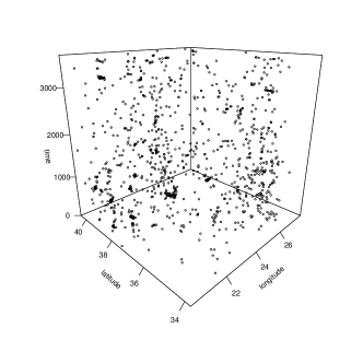
(a)

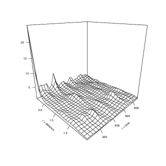
(b)

Figure 1: Earthquakes occurred in Greece between 2005 and 2014 (a); Pair correlation function of the observed point pattern (b).

We first consider a global LGCP with exponential covariance as in (1) using a joint estimation method as explained in Section 4.2. The corresponding spatial and temporal bandwidths are the same as indicated above in relation to Figure 1. We assume a constant intensity function estimated as $\hat{\lambda}(\textbf{u},t)=\hat{\lambda}=\frac{n}{|W\times T|}=0.006$. The estimates of the covariance parameters are $\hat{\boldsymbol{\psi}}=\{\hat{\sigma}^{2},\hat{\alpha},\hat{\beta}\}=\{6.14,0.27,449.55\}$, which indicate a quite clustered underlying process, given the high estimated variance, and the relatively small scale parameters.

To assess the goodness-of-fit of the proposed (global) model, a residual analysis is carried out by means of the Monte Carlo test based on the inhomogeneous $K$-functions outlined in Section 5. Figure 2(a) displays an example of LGCP point pattern simulated with the estimated parameters $\hat{\boldsymbol{\psi}}$, which is used to compute the envelopes for the test. Then, Figure 2(b) shows the the empirical $K$-function for the earthquake data, following (14), as well as the envelopes computed on $39$ simulations. A overall p-value of 0 is obtained from (15): being equal to zero indicates that the empirical pattern is not compatible with the simulated ones (that come from a LGCP with estimated parameters $\hat{\boldsymbol{\psi}}$). Therefore, the assumed model is not a good fit and an alternative should be searched, able to take into account the residual clustered behaviour of the points. Furthermore, Figure 2(b) confirms this result, as the observed $K$-function does not lie within the envelopes.

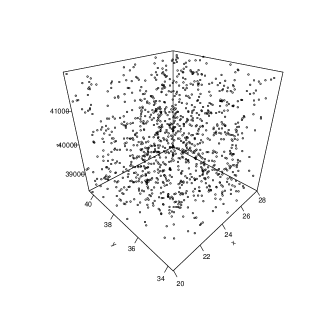
(a)

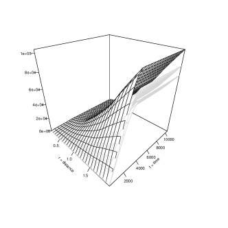
(b)

Figure 2: (a) An example of LGCP point pattern simulated with the estimated parameters $\hat{\boldsymbol{\psi}}$; (b) In black: the estimated weighted $K$-function for the Greek seismic data. In light grey: envelopes based on $39$ simulations from the global spatio-temporal LGCP at a significance level of 0.05.

We then consider a local spatio-temporal LGCP for the seismic data, and follow the locally weighted minimum contrast proposed in Section 4.3. The bandwidths $\epsilon$ and $\delta$, for the kernel in the pair correlation function, are the same used for the global fitting, while the bandwidths $\{\sigma_{x},\sigma_{y},\sigma_{t}\}$ for the local weighting are estimated to be $2.58,1.79$ and $1140.31$, for $x$, $y$, and $t$ coordinates, respectively. The results of the local fitting are shown in Table 3 and in Figure 3.

Table 3: Summary statistics of the estimated covariance parameters for the local LGCPs fitted to the Greek seismic data.

	$\hat{\sigma}^{2}$	$\hat{\alpha}$	$\hat{\beta}$
Min.	1.28	0.13	42.34
1st Qu.	5.19	0.25	366.43
Median	6.03	0.28	534.86
Mean	5.77	0.39	535.52
3rd Qu.	6.60	0.35	597.59
Max.	12.47	1.94	1411.45

As shown in Table 3, the proposed procedure provides a whole distribution for each parameter. Then, as evident from Figure 3, the estimated parameters allow to clearly distinguish different sub-areas where points behave differently from each other. Indeed, by inspection of the left panels of Figure 3, we can clearly spot two main spatial regions: the one on the top and on the left with higher $\hat{\sigma}_{i}^{2}$ values but lower estimates for $\hat{\alpha}_{i}$ and $\hat{\beta}_{i}$, and the area on the bottom-right which displays the opposite situation (low variance but large scale parameters).

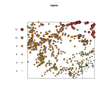
(a)

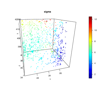
(b)

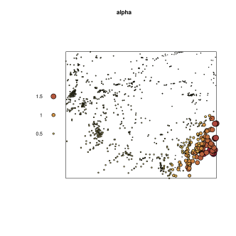
(c)

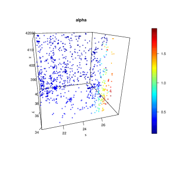
(d)

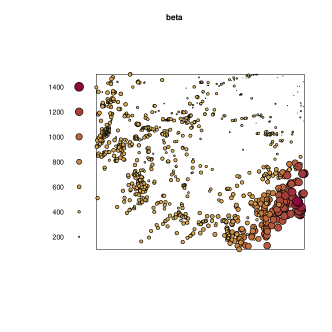
(e)

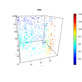
(f)

Figure 3: Local estimates of the local LGCP fitted to the Greek seismic data. We show a spatial representation on the left and a spatio-temporal one on the right.

This result is particularly appealing because it gives us more insight in the local behaviour of the seismic phenomenon. Indeed, from the global estimates we are only able to draw the conclusion that the analysed process is overall clustered. Conversely, the local application shows that earthquakes occurred on the top-left of the analysed area are grouped in smaller clusters, while the ones on the bottom-left have a way more diffuse clustering behaviour.

Furthermore, by looking at the right panels of Figure 3, we can assess also the time-varying behaviour of the estimates and therefore on the underlying process: the most relevant result concerns the variability of the covariance parameters $\hat{\sigma}_{i}$ in time, indicating that the number of earthquakes tends to increase in time, and in particular, in the top-left spatial region.

To assess whether the local model is a better fit to the data, also compared to the global counterpart, we proceed with the residual analysis as outlined in Section 5. For the local LGCP, the procedure is based on the modification of the GRF to be used to generate the point patterns, allowing to include information of the local estimates. To show the difference between the global and local GRFs, Figure 4 displays the spatial GRFs for three temporal instants, global and local, in the upper and lower panels, respectively. As evident, the local GRFs contain information about the local estimates, which in turn result in local variations.

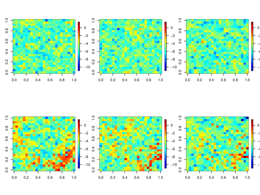
(a)

Figure 4: GRFs for three temporal instants: Top panels: global; Bottom panels: local.

Finally, Figure 5(a) displays an example of point pattern simulated with the estimated local parameters $\hat{\boldsymbol{\psi}}_{i}$, while Figure 5(b) depicts the estimated $K$-function and the envelopes computed from $39$ local simulations. It is worth noticing how the point pattern simulated from the local parameters, following our procedure, better mimics the spatio-temporal arragement of the original points (Figure 1(a)), if compared to the globally simulated point patterns (Figure 2(a)). An overall p-value of $0.28$ is obtained using the Monte Carlo local test, indicating that the patterns simulated from the assumed model (with the local estimated parameters) do not present any residual clustering behaviour. Therefore, we can conclude that the local model is a good fit to the analysed data. This result is further confirmed by Figure 5 (b), as now the observed $K$-function lies almost entirely between the envelopes obtained from the local simulation. Moreover, the local model also represents a better fit than its previously fitted global counterpart.

(a)

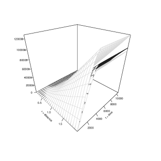
(b)

Figure 5: (a) A point pattern simulated with the estimated parameters $\hat{\boldsymbol{\psi}}_{i}$; (b) In black: the estimated inhomogeneous $K$-function for the Greek seismic data. In light grey: envelopes based on 39 simulations from the local spatio-temporal LGCP at a significance level of 0.05.

8 Conclusions

We have introduced a novel local fitting procedure for obtaining space-time local parameters for a log-Gaussian Cox process. From a methodological point of view, we have resorted to the joint minimum contrast procedure (which is appealing for its flexibility in dealing also with non-separable covariances), extending it to the local context, and therefore allowing to obtain a whole set of covariance parameters for each point of the analysed process. The motivating problem came from the seismic application, where of course it is of interest studying the characteristics of the process in relation to both the spatial and the temporal occurrence of points. By simulations, we have shown that the local proposal provides good estimates on average, if compared to the global fitting alternatives. Focussing on the application to real seismic data we have been able to assess that a local LGCP can be a better fit to the data if compared to its global counterpart. This is an expected result as the local fitting is based on a weighting given by a non-parametric estimate. However, our proposal presents further advantages than non-parametric alternatives, as it allows to obtain and interpret local parameters.

Our proposal poses the basis for many further investigations and applications. Indeed, in the future, the proposed methodology could be applied to different real spatio-temporal point patterns, where it is of interest to study the characteristics of the underlying process, in relation to the spatial displacement and the temporal occurrence of points. Some examples may include seismology, forestry, criminology, or epidemiology.

Concerning the local LGCPs, it would be interesting to develop software to include external covariates into the first-order intensity and to propose diagnostic methods for the particular case of multiple covariates, as an extension to D’Angelo et al., 2022b . Indeed, few spatio-temporal point process models account for external covariates: see Adelfio and Chiodi, (2020) for the ETAS model, and D’Angelo et al., (2021) for the spatio-temporal Hawkes point process model adapted to events living on linear networks. However, to the best of our knowledge, none of the recent proposals provide local estimates of the model regression-type parameters.

The inclusion of covariates would further allow to explore and compare their effects both in global and local models. See for instance Fotheringham and Sachdeva, (2022), which discuss some examples of the spatial variant of the Simpson’s paradox, by local models for areal data. Indeed, there might be some cases where the spatial variations observed in the local estimates of some covariates could simply be due to some misspecification of the model form (such as omitting informative covariates), rather than to spatially inhomogeneous behaviour. The same issue could hold in some spatio-temporal contexts.

Moreover, future works could focus also on the use of other summary statistics, such as the $K$-function, into the local minimum contrast procedure. Suitable simulation studies could be carried out, and the performance of different local second-order summary statistics could be compared, as discussed in Davies and Hazelton, (2013).

A related issue concerns the weights given to the averaged summary statistic, which strictly speaking could need not be kernel estimates nor Gaussian ones. For instance, Zhuang, (2015) (which applies the weighted likelihood estimator to the spatio-temporal ETAS model to study the spatial variations of seismicity characteristics in the Japan region) chooses a two-dimensional step-wise kernel function based on concentric disjoint octagon rings. The optimal kernel function and bandwidth, not discussed in detail in this study, could be investigated in future research.

Furthermore, other Cox models estimation could be carried out by exploiting the proposed minimum contrast procedure based on local second-order summary statistics.

Founding

This work was supported by ’FFR 2021 GIADA ADELFIO’.

References

- Adelfio and Chiodi, (2020) Adelfio, G. and Chiodi, M. (2020). Including covariates in a space-time point process with application to seismicity. Statistical Methods & Applications, pages 1–25.
- Adelfio et al., (2020) Adelfio, G., Siino, M., Mateu, J., and Rodríguez-Cortés, F. J. (2020). Some properties of local weighted second-order statistics for spatio-temporal point processes. Stochastic Environmental Research and Risk Assessment, 34(1):149–168.
- Anselin, (1995) Anselin, L. (1995). Local indicators of spatial association-lisa. Geographical analysis, 27(2):93–115.
- Baddeley, (2017) Baddeley, A. (2017). Local composite likelihood for spatial point processes. Spatial Statistics, 22:261–295.
- Baddeley, (2019) Baddeley, A. (2019). spatstat.local: Extension to ’spatstat’ for Local Composite Likelihood. R package version 3.6-0.
- Baddeley et al., (2015) Baddeley, A., Rubak, E., and Turner, R. (2015). Spatial Point Patterns: Methodology and Applications with R. London: Chapman and Hall/CRC Press.
- Baddeley and Turner, (2005) Baddeley, A. and Turner, R. (2005). spatstat: An R package for analyzing spatial point patterns. Journal of Statistical Software, 12(6):1–42.
- Baddeley et al., (2005) Baddeley, A., Turner, R., Møller, J., and Hazelton, M. (2005). Residual analysis for spatial point processes. Journal of the Royal Statistical Society, Series B (Statistical Methodology), 67(5):617–666.
- Baddeley and Turner, (2000) Baddeley, A. and Turner, T. R. (2000). Pratical maximum pseudo likelihood for spatial point patterns (with discussion). Australian & New Zealand Journal of Statistics, 42(3):283–322.
- Baddeley et al., (2000) Baddeley, A. J., Møller, J., and Waagepetersen, R. (2000). Non-and semi-parametric estimation of interaction in inhomogeneous point patterns. Statistica Neerlandica, 54(3):329–350.
- Berman and Turner, (1992) Berman, M. and Turner, T. R. (1992). Approximating point process likelihoods with glim. Journal of the Royal Statistical Society: Series C (Applied Statistics), 41(1):31–38.
- Brix and Diggle, (2001) Brix, A. and Diggle, P. J. (2001). Spatiotemporal prediction for log-gaussian cox processes. Journal of the Royal Statistical Society: Series B (Statistical Methodology), 63(4):823–841.
- Choi and Hall, (1999) Choi, E. and Hall, P. (1999). Nonparametric approach to analysis of space-time data on earthquake occurrences. Journal of Computational and Graphical Statistics, 8(4):733–748.
- Daley and Vere-Jones, (2007) Daley, D. J. and Vere-Jones, D. (2007). An Introduction to the Theory of Point Processes. Volume II: General Theory and Structure. Springer-Verlag, New York, second edition.
- (15) D’Angelo, N., Adelfio, G., Abbruzzo, A., and Mateu, J. (2022a). Inhomogeneous spatio-temporal point processes on linear networks for visitors’ stops data. The Annals of Applied Statistics. Forthcoming.
- D’Angelo et al., (2021) D’Angelo, N., Payares, D., Adelfio, G., and Mateu, J. (2021). Self-exciting point process modelling of crimes on linear networks. Submitted.
- (17) D’Angelo, N., Siino, M., D’Alessandro, A., and Adelfio, G. (2022b). Local spatial log-gaussian cox processes for seismic data. Advances in Statistical Analysis. Forthcoming.
- Davies and Hazelton, (2013) Davies, T. M. and Hazelton, M. L. (2013). Assessing minimum contrast parameter estimation for spatial and spatiotemporal log-gaussian cox processes. Statistica Neerlandica, 67(4):355–389.
- De Cesare et al., (2002) De Cesare, L., Myers, D., and Posa, D. (2002). Fortran programs for space-time modeling. Computers & Geosciences, 28(2):205–212.
- De Iaco et al., (2002) De Iaco, S., Myers, D. E., and Posa, D. (2002). Nonseparable space-time covariance models: some parametric families. Mathematical Geology, 34(1):23–42.
- Diggle, (1979) Diggle, P. J. (1979). On parameter estimation and goodness-of-fit testing for spatial point patterns. Biometrics, pages 87–101.
- Diggle, (2013) Diggle, P. J. (2013). Statistical Analysis of Spatial and Spatio-Temporal Point Patterns. CRC Press.
- Diggle and Gratton, (1984) Diggle, P. J. and Gratton, R. J. (1984). Monte carlo methods of inference for implicit statistical models. Journal of the Royal Statistical Society: Series B (Methodological), 46(2):193–212.
- Diggle et al., (2013) Diggle, P. J., Moraga, P., Rowlingson, B., and Taylor, B. M. (2013). Spatial and spatio-temporal log-gaussian cox processes: extending the geostatistical paradigm. Statistical Science, 28(4):542–563.
- Eguchi, (1983) Eguchi, S. (1983). Second order efficiency of minimum contrast estimators in a curved exponential family. The Annals of Statistics, pages 793–803.
- Fotheringham and Sachdeva, (2022) Fotheringham, A. S. and Sachdeva, M. (2022). On the importance of thinking locally for statistics and society. Spatial Statistics, page 100601.
- Gabriel and Diggle, (2009) Gabriel, E. and Diggle, P. J. (2009). Second-order analysis of inhomogeneous spatio-temporal point process data. Statistica Neerlandica, 63(1):43–51.
- Gabriel et al., (2021) Gabriel, E., Diggle, P. J., Rowlingson, B., and Rodriguez-Cortes, F. J. (2021). stpp: Space-Time Point Pattern Simulation, Visualisation and Analysis. R package version 2.0-5.
- Gneiting et al., (2006) Gneiting, T., Genton, M. G., and Guttorp, P. (2006). Geostatistical space-time models, stationarity, separability, and full symmetry. Monographs On Statistics and Applied Probability, 107:151.
- Guan, (2006) Guan, Y. (2006). A composite likelihood approach in fitting spatial point process models. Journal of the American Statistical Association, 101(476):1502–1512.
- Illian et al., (2008) Illian, J., Penttinen, A., Stoyan, H., and Stoyan, D. (2008). Statistical Analysis and Modelling of Spatial Point Patterns, volume 70. John Wiley & Sons.
- Møller, (2003) Møller, J. (2003). Shot noise cox processes. Advances in Applied Probability, pages 614–640.
- Møller et al., (1998) Møller, J., Syversveen, A. R., and Waagepetersen, R. P. (1998). Log gaussian cox processes. Scandinavian journal of statistics, 25(3):451–482.
- Musmeci and Vere-Jones, (1986) Musmeci, F. and Vere-Jones, D. (1986). A variable-grid algorithm for smoothing clustered data. Biometrics, pages 483–494.
- Ogata and Katsura, (1991) Ogata, Y. and Katsura, K. (1991). Maximum likelihood estimates of the fractal dimension for random spatial patterns. Biometrika, pages 463–474.
- Padoan and Bevilacqua, (2015) Padoan, S. A. and Bevilacqua, M. (2015). Analysis of random fields using comprandfld. Journal of Statistical Software, 63(1):1–27.
- Pfanzagl, (1969) Pfanzagl, J. (1969). On the measurability and consistency of minimum contrast estimates. Metrika, 14(1):249–272.
- R Core Team, (2020) R Core Team (2020). R: A Language and Environment for Statistical Computing. R Foundation for Statistical Computing, Vienna, Austria.
- Raeisi et al., (2021) Raeisi, M., Bonneu, F., and Gabriel, E. (2021). A spatio-temporal multi-scale model for geyer saturation point process: application to forest fire occurrences. Spatial Statistics, 41:100492.
- Ripley, (1977) Ripley, B. D. (1977). Modelling spatial patterns (with discussion). Journal of the Royal Statistical Society Series B, 39(2):172–212.
- Schlather et al., (2015) Schlather, M., Malinowski, A., Menck, P. J., Oesting, M., and Strokorb, K. (2015). Analysis, simulation and prediction of multivariate random fields with package random fields. Journal of Statistical Software, 63(8):1–25.
- Sheather and Jones, (1991) Sheather, S. J. and Jones, M. C. (1991). A reliable data-based bandwidth selection method for kernel density estimation. Journal of the Royal Statistical Society. Series B (Methodological), 53(3):683–690.
- (43) Siino, M., Adelfio, G., and Mateu, J. (2018a). Joint second-order parameter estimation for spatio-temporal log-gaussian cox processes. Stochastic environmental research and risk assessment, 32(12):3525–3539.
- (44) Siino, M., Rodríguez-Cortés, F. J., Mateu, J., and Adelfio, G. (2018b). Testing for local structure in spatiotemporal point pattern data. Environmetrics, 29(5-6):e2463.
- Silverman, (1986) Silverman, B. W. (1986). Density Estimation for Statistics and Data Analysis, volume 26. Chapman and Hall/CRC, London.
- Tamayo-Uria et al., (2014) Tamayo-Uria, I., Mateu, J., and Diggle, P. J. (2014). Modelling of the spatio-temporal distribution of rat sightings in an urban environment. Spatial Statistics, 9:192–206.
- Tanaka et al., (2008) Tanaka, U., Ogata, Y., and Stoyan, D. (2008). Parameter estimation and model selection for neyman-scott point processes. Biometrical Journal: Journal of Mathematical Methods in Biosciences, 50(1):43–57.
- Wand, (2020) Wand, M. (2020). KernSmooth: Functions for Kernel Smoothing Supporting Wand & Jones (1995). R package version 2.23-17.
- Zhuang, (2015) Zhuang, J. (2015). Weighted likelihood estimators for point processes. Spatial Statistics, 14:166–178.
- Zhuang, (2020) Zhuang, J. (2020). Estimation, diagnostics, and extensions of nonparametric hawkes processes with kernel functions. Japanese Journal of Statistics and Data Science, 3(1):391–412.
- Zhuang et al., (2002) Zhuang, J., Ogata, Y., and Vere-Jones, D. (2002). Stochastic declustering of space-time earthquake occurrences. Journal of the American Statistical Association, 97(458):369–380.