Semi-Counterfactual Risk Minimization Via Neural Networks

Abstract

Counterfactual risk minimization is a framework for offline policy optimization with logged data which consists of context, action, propensity score, and reward for each sample point. In this work, we build on this framework and propose a learning method for settings where the rewards for some samples are not observed, and so the logged data consists of a subset of samples with unknown rewards and a subset of samples with known rewards. This setting arises in many application domains, including advertising and healthcare. While reward feedback is missing for some samples, it is possible to leverage the unknown-reward samples in order to minimize the risk, and we refer to this setting as semi-counterfactual risk minimization. To approach this kind of learning problem, we derive new upper bounds on the true risk under the inverse propensity score estimator. We then build upon these bounds to propose a regularized counterfactual risk minimization method, where the regularization term is based on the logged unknown-rewards dataset only; hence it is reward-independent. We also propose another algorithm based on generating pseudo-rewards for the logged unknown-rewards dataset. Experimental results with neural networks and benchmark datasets indicate that these algorithms can leverage the logged unknown-rewards dataset besides the logged known-reward dataset.

Keywords: Offline policy optimization, Counterfactual Risk Minimization, Unknown reward

1 Introduction

Offline policy learning from logged data is an important problem in reinforcement learning theory and practice. The logged known-reward dataset represents interaction logs of a system with its environment recording context, action, reward (feedback), and propensity scores, i.e., probability of the selection of action for a given context under logging policy. This setting has been considered in the literature in connection with contextual bandits and partially labeled observations, and is used in many real applications, e.g., recommendation systems (Aggarwal et al., 2016; Li et al., 2011), personalized medical treatments (Kosorok and Laber, 2019; Bertsimas et al., 2017) and personalized advertising campaigns (Tang et al., 2013; Bottou et al., 2013). However, there are two main obstacles to learning from logged known-rewards data: first, the observed reward is available for the chosen action only; and second, the logged data is taken under the logging policy, so it could be biased. Counterfactual Risk Minimization (CRM), a strategy for off-policy learning from logged known-rewards datasets, has been proposed by Swaminathan and Joachims (2015a) to tackle these challenges.

CRM has led to promising results in some settings, including advertising and recommendation systems. However, there are some scenarios where the logged known-reward dataset is generated in an uncontrolled manner, and it poses a major obstacle, such as unobserved rewards for some chosen context and action pairs. For example, consider an advertising system server where some ads (actions) are shown to different clients (contexts) according to a conditional probability (propensity score). Now, suppose that the connections between the clients and the server are corrupted momentarily such that the server does not receive any reward feedback, i.e., whether or not the user has clicked on some ads. Under this scenario, we have access to the data, including the chosen clients, the shown ads, and the probability of shown ads without any feedback (reward) from the client, in addition to some logged known-reward data from multiple clients. A similar scenario arises in personalized medical treatment, where a treatment (action) is applied to a patient (context) with a conditional probability (propensity score), and we would like to observe the outcome of such a treatment in the near future (e.g., two years), but it is possible that some patients may pass away due to other conditions, preventing us to have access to the treatment outcome. Likewise, there are various other scenarios where it may be difficult to obtain reward samples for some context and action (and propensity score) samples since it might be expensive or unethical, such as in robotics or healthcare.

We call Semi-CRM our approach to learning in these scenarios, where we have access to the logged unknown-reward (no feedback) dataset, besides the logged known-reward (feedback) dataset.

This paper proposes algorithms that try to leverage the logged unknown-reward and known-reward datasets in an off-policy optimization problem. The contributions of our work are as follows:

• We propose a novel upper bound on the true risk under the inverse propensity score (IPS) estimator, in terms of different divergences, including KL divergence and Reverse KL, which is tighter than the previous upper bound (Cortes et al., 2010) under some conditions.

• Inspired by the upper bound on the true risk under the IPS estimator, we propose regularization approaches based on KL divergence or Reverse KL divergence, which are independent of rewards and hence can be optimized using the logged unknown-reward dataset. We also propose a consistent and unbiased estimator of KL divergence and Reverse KL divergence using the logged unknown-reward dataset.

• Inspired by the pseudo-labeling approach in semi-supervised learning (Lee et al., 2013), we also propose another approach based on estimating the reward function using logged known-reward dataset in order to produce pseudo-rewards for the logged unknown-reward dataset. This enables us to apply the IPS estimator regularized by weighted cross-entropy to both logged known-reward and unknown-reward datasets by leveraging the pseudo-rewards.

• We present experiments on the different datasets to evaluate our algorithms, showing the versatility of our approaches using logged unknown-reward data in different scenarios.

2 Related Works

There are various methods that have been developed over the years to learn from the logged known-reward dataset. The two main approaches are the Direct method and CRM.

Direct Method: The direct method for off-policy learning from logged known-reward datasets is based on estimation of the reward function, followed by application of a supervised learning algorithm to the problem (Dudík et al., 2014). However, this approach fails to generalize well as shown by Beygelzimer and Langford (2009). Gao et al. (2022) proposed another direct oriented method for off-line policy learning using the self-training approaches in semi-supervised learning.

Counterfactual Risk Minimization: Another approach for off-policy learning from logged known-reward dataset is CRM  (Swaminathan and Joachims, 2015a). In particular, Joachims et al. (2018) proposed a new approach to train a neural network, where the output of the Softmax layer can be considered as policy, and the network is trained based on a loss function using the available logged known-reward dataset. Using the PAC-Bayesian approach for CRM, London and Sandler (2018) derived an upper bound on the population risk of the optimal policy in terms of KL divergence between prior and posterior distributions over the hypothesis space. CRM has also been combined with domain adversarial networks by Atan et al. (2018). Wu and Wang (2018) proposed a new framework for CRM based on regularization by Chi-square divergence between optimal policy and the logging policy, and a generative-adversarial approach is proposed to minimize the regularized empirical risk using the logged known-reward dataset. Xie et al. (2018) introduced the surrogate policy method in CRM. The combination of causal inference and counterfactual learning was studied by Bottou et al. (2013). Distributional robust optimization is applied in CRM by Faury et al. (2020). A lower bound on the expected reward in CRM under Self-normalized Importance Weighting is derived by Kuzborskij et al. (2021).

Importance Weighting: Importance weighting has been proposed for off-policy estimation and learning (Thomas et al., 2015; Swaminathan and Joachims, 2015a). Importance weighting has a large variance in many cases (Rosenbaum and Rubin, 1983); hence some truncated importance sampling methods are proposed, including the IPS estimator with truncated ratio of policy and logging policy (Ionides, 2008), IPS estimator with truncated propensity score (Strehl et al., 2010) or self-normalizing estimator (Swaminathan and Joachims, 2015b). Kallus (2018) proposed a balance-based weighting approach for policy learning which outperforms other estimators. A generalization of the importance sampling by considering samples from different policies is studied by Papini et al. (2019). The weights can be estimated directly by sampling from contexts and actions using Direct Importance Estimation (Sugiyama et al., 2007). In this work we consider IPS estimator based on truncated propensity score.

Individualized Treatment Effects: The aim of individual treatment effect is the estimation of the expected values of the squared difference between outcomes (rewards) for control and treated contexts (Shalit et al., 2017). In the individual treatment effect scenario, the actions are limited to two actions (treated/not treated) and the propensity scores are unknown (Shalit et al., 2017; Johansson et al., 2016; Alaa and van der Schaar, 2017). Our work differs from this line of works by considering more actions, and also we are focused on leveraging the availability of the logged unknown-reward dataset (in addition to the logged known-reward dataset).

Inverse Reinforcement Learning: Inverse RL, an approach to learn reward functions in a data-driven manner, has also been proposed to deal with unknown reward datasets in RL (Finn et al., 2016; Konyushkova et al., 2020; Abbeel and Ng, 2004). The identifiablity of reward function learning under entropy regularization is studied by Cao et al. (2021). Our work differs from this line of research, since we assume access to propensity score parameters, besides the context and action. Our logged known-reward and unknown-reward datasets are under a fixed logging policy for all samples.

Semi-Supervised Learning: There are some connections between our scenario, and semi-supervised learning (Yang et al., 2021) approaches, including entropy minimization and pseudo-labeling. In entropy minimization, an entropy function of predicted conditional distribution is added to the main empirical risk function, which depends on unlabeled data (Grandvalet et al., 2005). The entropy function can be viewed as an entropy regularization and can lower the entropy of prediction on unlabeled data. In Pseudo-labeling, the model is trained using labeled data in a supervised manner and is also applied to unlabeled data in order to provide a pseudo label with high confidence (Lee et al., 2013). These pseudo labels would be applied as inputs for another model, trained based on labeled and pseudo-label data in a supervised manner. Our work differs from semi-supervised learning as the logging policy biases our logged data, and the rewards for other actions are not available. In semi-supervised learning, the label is unknown for some of the data. In comparison, in our setup, the reward is unknown.

3 Preliminaries

Notations: We adopt the following convention for random variables and their distributions in the sequel. A random variable is denoted by an upper-case letter (e.g. $Z$), its space of possible values is denoted with the corresponding calligraphic letter (e.g. $\mathcal{Z}$), and an arbitrary value of this variable is denoted with the lower-case letter (e.g. $z$). This way, we can describe generic events like $\{Z=z\}$ for any $z\in\mathcal{Z}$, or events like $\{g(Z)\leq 5\}$ for functions $g:\mathcal{Z}\to\mathbb{R}$. The probability distribution of the random variable $Z$ is denoted by $P_{Z}$. The joint distribution of a pair of random variables $(Z_{1},Z_{2})$ is denoted by $P_{Z_{1},Z_{2}}$. We denote the set of integer numbers from 1 to $n$ by $[n]\triangleq\{1,\cdots,n\}$.

Divergence Measures: If $P$ and $Q$ are probability measures over $\mathcal{Z}$, the Kullback-Leibler (KL) divergence between $P$ and $Q$ is given by $D(P\|Q)\triangleq\int_{\mathcal{Z}}\log\bigl{(}\frac{dP}{dQ}\bigr{)}dP$ when $P$ is absolutely continuous with respect to $Q$, and $D(P\|Q)\triangleq\infty$ otherwise; it measures how much $Q$ differs from $P$ in the sense of statistical distinguishability (Csiszár and Körner, 2011). The reverse KL divergence between $P$ and $Q$ is given by $D_{r}(P\|Q)\triangleq\int_{\mathcal{Z}}\log\bigl{(}\frac{dQ}{dP}\bigr{)}dQ=D(Q\|P)$, and the conditional KL divergence between $P_{T|Z}$ and $Q_{T}$ averaged over $P_{Z}$ is given by $D(P_{T|Z}\|Q_{T}|P_{Z})\triangleq\int_{\mathcal{Z}}D(P_{T|Z=z}\|Q_{T})dP_{Z}(z)$. The chi-square divergence between $P$ and $Q$ is given by $\chi^{2}(P\|Q)\triangleq\int_{\mathcal{Z}}(\frac{dP}{dQ})^{2}dQ-1$.

Problem Formulation Let $\mathcal{X}$ be the set of contexts and $\mathcal{A}$ the finite set of actions, with $|\mathcal{A}|=k$. We consider policies as conditional distributions over actions given contexts. For each pair of context and action $(x,a)\in\mathcal{X}\times\mathcal{A}$ and policy $\pi\in\Pi$, where $\Pi$ is the set of policies, the value $\pi(a|x)$ is defined as the conditional probability of choosing action $a$ given context $x$ under the policy $\pi$.

A reward function $f_{r}:\mathcal{X}\times\mathcal{A}\rightarrow[-1,0]$, which is unknown, defines the reward of each observed pair of context and action. However, in a logged known-reward setting we only observe the reward (feedback) for the chosen action $a$ in a given context $x$, under the logging policy $\pi_{0}(a|x)$. We have access to the the logged known-reward dataset $S=(x_{i},a_{i},p_{i},r_{i})_{i=1}^{n}$ where each ‘data point’ $(x_{i},a_{i},p_{i},r_{i})$ contains the context $x_{i}$ which is sampled from unknown distribution $P_{X}$, the action $a_{i}$ which is sampled from (unknown) logging policy $\pi_{0}(\cdot|x_{i})$, the propensity score $p_{i}\triangleq\pi_{0}(a_{i}|x_{i})$, and the observed reward $r_{i}\triangleq f_{r}(x_{i},a_{i})$ under logging policy $\pi_{0}(a_{i}|x_{i})$.

In this work, inspired by the BanditNet method of Swaminathan and Joachims (2015b), we use a neural network with parameters $\theta$ to model a stochastic policy $\pi_{\theta}$. For example, we can use the output of a Softmax layer in a neural network, to define as a stochastic policy as follows:

$$\pi_{\theta}(a_{i}|x)=\frac{\exp(h_{\theta}(x,a_{i}))}{\sum_{i=1}^{k}\exp(h_{\theta}(x,a_{i}))},$$ (1)

where $h_{\theta}(a_{i},x)$ is the $i$-th input to Softmax layer for context $x\in\mathcal{X}$ and action $a_{i}\in\mathcal{A}$.

The true risk of a policy $\pi_{\theta}$ is defined as follows:

$$R(\pi_{\theta}) =\mathbb{E}_{P_{X}}[\mathbb{E}_{\pi_{\theta}(A|X)}[f_{r}(X,A)]].$$ (2)

Our objective is to find an optimal $\pi_{\theta}^{\star}$ which minimizes $R(\pi_{\theta})$, i.e.,

$$\pi_{\theta}^{\star}=\arg\min_{\pi_{\theta}\in\Pi_{\theta}}R(\pi_{\theta}),$$ (3)

where $\Pi_{\theta}$ is the set of all policies parameterized by $\theta$. We denote the importance weighted reward function as $w(A,X)f_{r}(A,X)$, where $w(A,X)=\frac{\pi_{\theta}(A|X)}{\pi_{0}(A|X)}.$

As discussed by Swaminathan and Joachims (2015b), we can apply IPS estimator over logged known-reward dataset $S$ (Rosenbaum and Rubin, 1983) to get an unbiased estimator of the risk (an empirical risk) by considering the importance weighted reward function as follows:

$$\hat{R}(\pi_{\theta},S) =\frac{1}{n}\sum_{i=1}^{n}r_{i}w(a_{i},x_{i}),$$ (4)

where $w(a_{i},x_{i})=\frac{\pi_{\theta}(a_{i}|x_{i})}{p_{i}}$ and $p_{i}=\pi_{0}(a_{i}|x_{i})$. The IPS estimator as unbiased estimator has bounded variance if the $\pi_{\theta}(A|X)$ is absolutely continuous with respect to $\pi_{0}(A|X)$ (Strehl et al., 2010; Langford et al., 2008). For the issue of the large variance of the IPS estimator, many estimators exist,  (Strehl et al., 2010; Ionides, 2008; Swaminathan and Joachims, 2015b), e.g., truncated IPS estimator. In this work we consider truncated IPS estimator with $\zeta\in[0,1]$ as follows:

$$\hat{R}^{\zeta}(\pi_{\theta},S) =\frac{1}{n}\sum_{i=1}^{n}r_{i}\frac{\pi_{\theta}(a_{i}|x_{i})}{\max(p_{i},\zeta)},$$ (5)

In our Semi-CRM setting, we also have access to the logged unknown-reward dataset, which we shall denote as $S_{u}=(x_{j},a_{j},p_{j})_{j=1}^{m}$ which is generated under the same logging policy for logged known-reward dataset, i.e., $p_{j}=\pi_{0}(a_{j}|x_{j})$. We will next propose two algorithms to derive a policy which minimize the true risk using logged unknown-reward and known-reward datasets.

4 Bounds on Variance of Importance Weighted Reward Function

In this section, we provide upper and lower bounds on variance of importance weighted reward function, i.e.,

$$\operatorname{Var}\left(w(A,X)f_{r}(A,X)\right)\triangleq\mathbb{E}_{P_{X}\otimes\pi_{0}(A|X)}\left[\left(w(A,X)f_{r}(A,X)\right)^{2}\right]-R^{2}(\pi_{\theta})$$ (6)

where $R^{2}(\pi_{\theta})=\mathbb{E}_{P_{X}\otimes\pi_{0}(A|X)}\left[w(A,X)f_{r}(A,X)\right]^{2}$.

Proposition 1

(proved in Appendix A) Suppose that the importance weighted of squared reward function, namely, $w(A,X)f_{r}^{2}(A,X)$, is $\sigma$-sub-Gaussian under $P_{X}\otimes\pi_{0}(A|X)$ and $P_{X}\otimes\pi_{\theta}(A|X)$, the reward function, $f_{r}(A,X)$, is bounded in $[c,b]$, and $b\geq 0$. Then the following upper bound holds on the variance of the importance weighted reward function:

$$\operatorname{Var}\left(w(A,X)f_{r}(A,X)\right)\leq\sqrt{2\sigma^{2}\min(D(\pi_{\theta}\|\pi_{0}),D_{r}(\pi_{\theta}\|\pi_{0}))}+b_{u}^{2}-c_{l}^{2},$$ (7)

where $D(\pi_{\theta}\|\pi_{0})=D(\pi_{\theta}(A|X)\|\pi_{0}(A|X)|P_{X})$ and $D_{r}(\pi_{\theta}\|\pi_{0})=D_{r}(\pi_{\theta}(A|X)\|\pi_{0}(A|X)|P_{X})$; and the constants $c_{l}=\max(c,0)$ and $b_{u}=\max(|c|,b)$,.

Note that if $\sup_{(x,a)\in\mathcal{X}\times\mathcal{A}}w(a,x)=w_{m}<\infty$, then we have $\sigma=\frac{w_{m}b_{u}^{2}}{2}$ under both distributions, $P_{X}\otimes\pi_{0}(A|X)$ and $P_{X}\otimes\pi_{\theta}(A|X)$ in Proposition 1.

Using Cortes et al. (2010, Lemma 1), we can provide an upper bound on the variance of importance weights in terms of chi-square divergence by considering $f_{r}(a,x)\in[c,b]$, as follows:

$$\operatorname{Var}\left(w(A,X)f_{r}(A,X)\right)\leq b_{u}^{2}\chi^{2}(\pi_{\theta}(A|X)\|\pi_{0}(A|X)|P_{X})+b_{u}^{2}-c_{l}^{2},$$ (8)

where $c_{l}=\max(c,0)$, $b_{u}=\max(|c|,b)$. In Appendix C, we discuss that under some conditions, the upper bound in Proposition 1 is tighter than the upper bound based on chi-square divergence (8). A lower bound on the variance of importance weighted reward function in terms of KL divergence between $\pi_{\theta}$ and $\pi_{0}$ is provided in the following Proposition.

Proposition 2

(proved in Appendix A) Suppose that $q\leq e^{\mathbb{E}_{P_{X}\otimes\pi_{\theta}(A,X)}[\log(|f_{r}(A,X)|)]}$, $f_{r}(a,x)\in[c,b]$ and $b\geq 0$. Then, following lower bound holds on the variance of importance weighted reward function,

$$\operatorname{Var}\left(w(A,X)f_{r}(A,X)\right)\geq q^{2}e^{D(\pi_{\theta}(A|X)\|\pi_{0}(A|X)|P_{X})}-b_{u}^{2}.$$ (9)

where $b_{u}=\max(|c|,b)$.

The upper bound in Proposition 1 shows that we can reduce the variance of importance weights, i.e., $w(A,X)$, by minimizing the KL divergence or reverse KL divergence between $\pi_{\theta}$ and $\pi_{0}$. The lower bound on the variance of importance weights in Proposition 2 can be minimized by minimizing the KL divergence between $\pi_{\theta}$ and $\pi_{0}$.

5 Semi-CRM Algorithms

We now propose two approaches: reward-free regularized CRM and Semi-CRM via Pseudo-rewards, which are capable of leveraging the availability of both the logged known-reward dataset $S$ and the logged unknown-reward dataset $S_{u}$. The reward-free regularized CRM is based on the optimization of a regularized CRM where the regularization function is independent of the rewards. The reward-free regularized CRM is inspired by an entropy minimization approach in semi-supervised learning, where one optimizes a label-free entropy function using the unlabeled data. In the Semi-CRM via pseudo-rewards, inspired by the Pseudo-labeling algorithm in semi-supervised learning, a model based on the logged known-reward dataset is incorporated to assign pseudo-rewards to logged unknown-reward dataset, and then the final model is trained using based on the logged known-reward dataset and logged unknown-reward dataset augmented by pseudo-rewards. These two approaches are described in the following two sections.

5.1 Semi-CRM via Reward-free Regularization

In this section, we start by providing an upper bound on the true risk under the importance weighting method, which shows that we can control the variance of the weighted reward function by tuning the KL divergence or reverse KL divergence between the optimal and logging policies. Then, we propose regularizers based on the KL divergence and reverse KL divergence, independent of the reward function, that can be optimized using the logged unknown-reward dataset.

Using the upper bound on the variance of importance weighted reward function in Proposition 1, we can derive a high-probability bound on the true risk under the importance weighting method.

Theorem 3

(proved in Appendix B) Suppose the reward function takes values in $[-1,0]$. Then, for any $\delta\in(0,1)$, the following bound on the true risk based on the importance weighting method holds with probability at least $1-\delta$ under the distribution $P_{X}\otimes\pi_{0}(A|X)$:

$$R(\pi_{\theta})\leq\hat{R}(\pi_{\theta},S)+\frac{w_{m}\log(\frac{1}{\delta})}{3n}+\sqrt{\frac{(w_{m}\sqrt{2\min(D(\pi_{\theta}\|\pi_{0}),D_{r}(\pi_{\theta}\|\pi_{0}))}+2)\log(\frac{1}{\delta})}{n}}$$ (10)

where $D(\pi_{\theta}\|\pi_{0})=D(\pi_{\theta}(A|X)\|\pi_{0}(A|X)|P_{X})$ and $D_{r}(\pi_{\theta}\|\pi_{0})=D_{r}(\pi_{\theta}(A|X)\|\pi_{0}(A|X)|P_{X})$, and the uniform bound on the importance weights $w_{m}=\sup_{(x,a)\in\mathcal{X}\times\mathcal{A}}w(a,x)<\infty$.

The proof of Theorem 3 leverages the Bernstein inequality together with an upper bound on the variance of importance weighted reward function using Proposition 1. The Theorem 3 shows that we can minimize the KL divergence between $\pi_{\theta}$ and $\pi_{0}$, i.e., $D(\pi_{\theta}(A|X)\|\pi_{0}(A|X)|P_{X})$, or reverse KL divergence between $\pi_{\theta}$ and $\pi_{0}$, i.e., $D_{r}(\pi_{\theta}(A|X)\|\pi_{0}(A|X)|P_{X})$, instead of empirical variance minimization in CRM framework (Swaminathan and Joachims, 2015a) which is inspired by the upper bound in Maurer and Pontil (2009).

Note that the KL divergence and reverse KL divergence between logging policy and the true policy are independent from the reward function values (feedback). This motivates us to consider them as functions which can be optimized using the logged unknown-reward dataset. It is worthwhile mentioning that the regularization based on empirical variance in Swaminathan and Joachims (2015a) is dependent on reward.

Now, inspired by the semi-supervised frameworks in Aminian et al. (2022); He et al. (2021), we propose the following convex combination of empirical risk and KL divergence or Reverse KL divergence for Semi-CRM problem:

$$\hat{R}_{\mathrm{KL}}(\pi_{\theta},S,S_{u})\triangleq\alpha\hat{R}(\pi_{\theta},S)+(1-\alpha)D(\pi_{\theta}(A|X)\|\pi_{0}(A|X)|P_{X}),\quad\alpha\in[0,1],$$ (11)

$$\hat{R}_{\mathrm{RKL}}(\pi_{\theta},S,S_{u})\triangleq\alpha\hat{R}(\pi_{\theta},S)+(1-\alpha)D_{r}(\pi_{\theta}(A|X)\|\pi_{0}(A|X)|P_{X}),\quad\alpha\in[0,1],$$ (12)

where for $\alpha=1$, our problem reduces to traditional CRM that neglects the logged unknown-reward dataset, whereas for $\alpha=0$, we solely optimise the KL divergence or reverse KL divergence using logged unknown-reward dataset. More discussion for KL regularization is provided in Appendix G.

For the estimation of $D(\pi_{\theta}(A|X)\|\pi_{0}(A|X)|P_{X})$ and $D_{r}(\pi_{\theta}(A|X)\|\pi_{0}(A|X)|P_{X})$, we can apply the logged unknown-reward dataset as follows:

$$\hat{R}_{\mathrm{KL}}(\pi_{\theta},S_{u})\triangleq\sum_{i=1}^{k}\frac{1}{m_{[i]}}\sum_{(x,a_{i},p)\in S_{u}}\pi_{\theta}(a_{i}|x)\log(\frac{\pi_{\theta}(a_{i}|x)}{p}),$$ (13)

$$\hat{R}_{\mathrm{RKL}}(\pi_{\theta},S_{u})\triangleq\sum_{i=1}^{k}\frac{1}{m_{[i]}}\sum_{(x,a_{i},p)\in S_{u}}-p\log(\pi_{\theta}(a_{i}|x))+p\log(p),$$ (14)

where $m_{[i]}$ is the number of context, action and propensity score tuples, i.e., $(x,a,p)\in S_{u}$, with the same action, e.g., $a=a_{i}$ (note we have $\sum_{i=1}^{k}m_{[i]}=m$). It is possible to show that the estimations of KL divergence and reverse KL divergence are unbiased in asymptotic regime.

Proposition 4

(proved in Appendix B) Suppose that the KL divergence and reverse KL divergence between $\pi_{\theta}$ and $\pi_{0}$ are bounded. Assuming $m_{[i]}\rightarrow\infty$ $(\forall i\in[k])$, $\hat{R}_{\mathrm{KL}}(\pi_{\theta},S_{u})$ and $\hat{R}_{\mathrm{RKL}}(\pi_{\theta},S_{u})$ are unbiased estimations of $D(\pi_{\theta}(A|X)\|\pi_{0}(A|X)|P_{X})$ and $D_{r}(\pi_{\theta}(A|X)\|\pi_{0}(A|X)|P_{X})$, respectively.

Note that another approach to minimize the KL divergence or reverse KL divergence is the generative-adversarial approach in (Wu and Wang, 2018) which is based on using logged known-reward dataset without considering rewards and propensity scores. It is worthwhile to mention that the generative-adversarial approach will not consider propensity scores in the logged known-reward dataset and also incur more complexity, including Gumbel soft-max sampling (Jang et al., 2016) and discriminator network optimization. We proposed a new estimator of these information measures considering our access to propensity scores in the logged unknown-reward dataset. Since the term $p\log(p)$ in (14) is independent of policy $\pi_{\theta}$, we ignore it and optimize the following quantity instead of $\hat{R}_{\mathrm{RKL}}(\pi_{\theta},S_{u})$ which is similar to cross-entropy by considering propensity scores as weights of cross-entropy:

$$\hat{R}_{\mathrm{WCE}}(\pi_{\theta},S_{u})\triangleq\sum_{i=1}^{k}\frac{1}{m_{[i]}}\sum_{(x,a_{i},p)\in S_{u}}-p\log(\pi_{\theta}(a_{i}|x)),$$ (15)

In the following, we also provide another interpretation for KL divergence and reverse KL divergence between $\pi_{\theta}$ and $\pi_{0}$.

Proposition 5

(proved in Appendix B) The following upper bound holds on the absolute difference between risks of logging policy, $\pi_{0}(a|x)$, and the policy, $\pi_{\theta}(a|x)$:

$$|R(\pi_{\theta})-R(\pi_{0})|\leq\min\left(\sqrt{\frac{D(\pi_{\theta}\|\pi_{0})}{2}},\sqrt{\frac{D_{r}(\pi_{\theta}\|\pi_{0})}{2}}\right)$$ (16)

where $D(\pi_{\theta}\|\pi_{0})=D(\pi_{\theta}(A|X)\|\pi_{0}(A|X)|P_{X})$ and $D_{r}(\pi_{\theta}\|\pi_{0})=D_{r}(\pi_{\theta}(A|X)\|\pi_{0}(A|X)|P_{X})$.

Based on Proposition 5, the minimization of KL divergence and reverse KL divergence would lead to a policy close to the logging policy in KL divergence or reverse KL divergence. This phenomena, which happens also observed in the works of Swaminathan and Joachims (2015a); Wu and Wang (2018); London and Sandler (2018), is aligned with the fact that the optimal policy’s action distribution should not diverge too much from the logging policy (Schulman et al., 2015).

For improvement in the scenarios where the propensity scores in the logged unknown-reward dataset are not clean, we use the propensity score truncation in (13) and (14) as follows:

$$\hat{R}_{\mathrm{KL}}^{\tau}(\pi_{\theta},S_{u})\triangleq\sum_{i=1}^{k}\frac{1}{m_{[i]}}\sum_{(x,a_{i},p)\in S_{u}}\pi_{\theta}(a_{i}|x)\log\left(\frac{\pi_{\theta}(a_{i}|x)}{\max(\tau,p)}\right)$$ (17)

$$\hat{R}_{\mathrm{WCE}}^{\tau}(\pi_{\theta},S_{u})\triangleq\sum_{i=1}^{k}\frac{1}{m_{[i]}}\sum_{(x,a_{i},p)\in S_{u}}-\max(\tau,p)\log(\pi_{\theta}(a_{i}|x))$$ (18)

where $\tau\in[0,1]$. For $\tau=1$, we actually do not consider the propensity scores, and for $\tau=0$ we actually consider clean propensity scores. In a case of $p_{i}=0$ for a sample $(x_{i},a_{i},p_{i})\in S_{u}$, we have $\hat{R}_{\mathrm{KL}}=-\infty$, hence considering $\tau$ in $\hat{R}_{\mathrm{KL}}$, will also help to solve these cases. Since $\max(\tau,p)\geq p$, we have that $\hat{R}_{\mathrm{WCE}}^{\tau}(\pi_{\theta},S_{u})\geq\hat{R}_{\mathrm{WCE}}(\pi_{\theta},S_{u})$, $\forall\tau\in[0,1]$. Thus, by minimizing $\hat{R}_{\mathrm{WCE}}^{\tau}(\pi_{\theta},S_{u})$, we minimize an upper bound on $\hat{R}_{\mathrm{WCE}}(\pi_{\theta},S_{u})$, as a sub-optimal solution. A complete training algorithm, i.e., WCE-CRM algorithm, based on reward-free regularization CRM via truncated weighted cross-entropy is proposed in Algorithm 1. The KL-CRM algorithm as a regularized CRM based on estimation of KL divergence between $\pi_{\theta}$ and $\pi_{0}$ is similar to Algorithm 1 by replacing $R_{\mathrm{WCE}}^{\tau}(\theta^{t_{g}})$ with $R_{\mathrm{KL}}^{\tau}(\theta^{t_{g}})$ defined as:

$$R_{\mathrm{KL}}^{\tau}(\theta^{t_{g}})=\sum_{i=1}^{k}\frac{1}{m_{[i]}}\sum_{(x,a_{i},p)\in S_{u}}\pi_{\theta^{t_{g}}}(a_{i}|x)\log\left(\frac{\pi_{\theta^{t_{g}}}(a_{i}|x)}{\max(\tau,p)}\right).$$ (19)

Data: $S=(x_{i},a_{i},p_{i},r_{i})_{i=1}^{n}$ sampled from $\pi_{0}$, $S_{u}=(x_{j},a_{j},p_{j})_{j=1}^{m}$ sampled from $\pi_{0}$, hyper-parameters $\alpha$, $\zeta$ and $\tau$, initial policy $\pi_{\theta^{0}}(a|x)$, and max epochs for the whole algorithm $M$

Result: An optimized neural network $\pi^{\star}_{\theta}(a|x)$ which minimize the regularized risk by truncated weighted cross-entropy

while epoch $\leq M$ do

       Sample $n_{1}$ samples $(x_{i},a_{i},p_{i},r_{i})$ from $S$ and estimate the re-weighted loss as $\hat{R}^{\zeta}(\theta^{t_{g}})=\frac{1}{n_{1}}\sum_{i=1}^{n_{1}}r_{i}\frac{\pi_{\theta^{t_{g}}}(a_{i}|x_{i})}{\max(\zeta,p_{i})}$

      

      Get the gradient with respect to $\theta^{t_{g}}$ as $g_{1}\leftarrow\nabla_{\theta^{t_{g}}}\hat{R}^{\zeta}(\theta^{t_{g}})$

       Sample $m_{1}$ samples from $S_{u}$ and estimate the weighted cross-entropy loss ($\sum_{i=1}^{k}m_{[i]}=m_{1}$)

      

      $R_{\mathrm{WCE}}^{\tau}(\theta^{t_{g}})=\sum_{i=1}^{k}\frac{1}{m_{[i]}}\sum_{(x,a_{i},p)\in S_{u}}-\max(\tau,p)\log(\pi_{\theta^{t_{g}}}(a_{i}|x))$

      

      Get the gradient with respect to $\theta^{t_{g}}$ as $g_{2}\leftarrow\nabla_{\theta^{t_{g}}}R_{\mathrm{WCE}}^{\tau}(\theta^{t_{g}})$

      

      Update $\theta^{t_{g}+1}=\theta^{t_{g}}-(\alpha g_{1}+(1-\alpha)g_{2})$

end while

Algorithm 1 WCE-CRM Algorithm

5.2 Semi-CRM via Pseudo-rewards

In this section, we introduce a Semi-CRM approach that leverage pseudo-rewards, inspired by the pseudo-label mechanism in semi-supervised learning and also the work by Konyushkova et al. (2020).

The logged known-reward dataset can help to learn a reward-regression model to predict the rewards of the logged unknown-reward dataset. For this purpose, we can use the weighted least square objective function (Cleveland and Devlin, 1988) over a linear class ($\mathcal{C}^{l}$) of regressors to train the reward regression model using the logged known-reward dataset, $S$, as follows:

$$\hat{f}_{r}(x,a)=\arg\min_{\hat{f}_{r}\in\mathcal{C}^{l}}\frac{1}{\mathrm{P}}\sum_{i=1}^{n}p_{i}(r_{i}-\hat{f}_{r}(x_{i},a_{i}))^{2}$$ (20)

where $\mathrm{P}=\sum_{i=1}^{n}p_{i}$. The Neural networks can also be applied to estimate the reward function as a regression problem. Now, the reward regression model $\hat{f}_{r}(x,a)$ can be applied to the unknown reward dataset to predict the pseudo-reward $\hat{r}_{i}$ given the context $x_{i}$ and action $a_{i}$, leading up to augmenting each sample $(x_{i},a_{i},p_{i},\hat{r}_{i})$. It is worthwhile to mention that, as the underlying policy of the unknown reward dataset is the same as the known reward dataset, i.e., logging policy $\pi_{0}$, we do not have the bias problem in dataset (Dudík et al., 2014). Using the known reward dataset, $S$, and augmented logged unknown-reward dataset by pseudo-rewards, we can then train the model by applying the CRM approach, which is regularized by weighted cross-entropy over both datasets to reduce the variance of the IPS estimator. The Pseudo-reward risk function, i.e., $\hat{R}_{PR}(\pi_{\theta},S,S_{u})\triangleq$, is as follows:

$$\frac{\alpha}{n+m}\left(\sum_{i=1}^{n}r_{i}\frac{\pi_{\theta}(a_{i}|x_{i})}{\max(\zeta,p_{i})}+\sum_{j=1}^{m}\hat{r}_{j}\frac{\pi_{\theta}(a_{j}|x_{j})}{\max(\zeta,p_{j})}\right)+(1-\alpha)\hat{R}^{\tau}_{\mathrm{WCE}}(\pi_{\theta},S_{u}\cup S)$$ (21)

where $\hat{R}^{\tau}(\pi_{\theta},S_{u}\cup S)=\sum_{i=1}^{k}\frac{-1}{m_{[i]}}\sum_{(x,a_{i},p)\in S_{u}\cup S}\max(\tau,p)\log(\pi_{\theta}(a_{i}|x))$ and $\alpha\in[0,1]$. The training algorithm for semi-CRM based on the pseudo-reward approach, PR-CRM, is proposed in Appendix D.

6 Experiments

We evaluated the performance of the algorithms WCE-CRM, KL-CRM, and PR-CRM by applying the standard supervised to bandit transformation (Beygelzimer and Langford, 2009) on two image classification datasets: Fashion-MNIST (Xiao et al., 2017) and CIFAR-10 (Krizhevsky et al., 2009). This transformation assumes that each of the ten classes in the datasets corresponds to an action. Then, a logging policy stochastically selects an action for every instance in the dataset. Finally, if the selected action matches the actual label assigned to the instance, then we have $r=-1$, and $r=0$ otherwise. Similar to the work of London and Sandler (2018), we evaluated the performance of the different algorithms in terms of expected risk and accuracy. The expected risk is the average of the reward function over the test set, while the accuracy is simply the proportion of times where the action with $r=-1$ is equal to the action with a deterministic argmax policy.

To learn the logging policy, we trained the first seven convolutional and the two last fully connected layers of the VGG-16 architecture (Simonyan and Zisserman, 2014) with $5\%$ of the available training data in each dataset. The last hidden layer contained 25 neurons, while the output layer contained ten neurons and used a soft-max activation function. Once learned, we used the logging policy to create the logged known-reward datasets using the remaining 95% of the instances in the datasets. We trained the model for five epochs for the Fashion-MNIST dataset and 50 epochs for the CIFAR-10 datasets. Each instance in the logged known-reward datasets is a 4-tuple $(x,a,p,r)$, where $x$ is the output of the last hidden layer of the network used to compute the logging policy. In this case, it is a 25-dimensional vector representing the embedding of an image, and $a$ is a stochastically selected action, $p$ is the value of the output layer of the selected action, and $r$ is the reward.

To simulate the absence of rewards for logged known-reward datasets, we pretended that the reward was not available in 90% of the instances in each dataset, while the reward of remaining 10% was known. The policy $\pi_{\theta}(a\ |\ x)$ was implemented using a fully connected neural network with 2 hidden layers and ReLU activation functions, and an output layer with softmax activation function. The network for both Fashion-MNIST and CIFAR-10 has 20 neurons per layer. We trained the networks using the WCE-CRM, KL-CRM and PR-CRM algorithms with $M=1000,n=5700,m=51300$. In PR-CRM, the pseudo rewards are generated using the estimation of reward function (20).

Figure 1 shows the average expected risk, over 10 runs, of applying PR-CRM, WCE-CRM and KL-CRM algorithms to the Fashion-MNIST and CIFAR-10 datasets using different values for the regularization parameter $\alpha$ by considering $\tau=\zeta=0.001$ as truncation hyper-parameters (chosen via cross validation). We also included the result for BandiNet trained based on 10% of each dataset by assuming reward is known, and the result for supervised approach, where the network is trained by access to full supervised dataset. The error bars represent the standard deviation over the 10 runs. Figure 2 shows similar graphs, but in terms of accuracy.

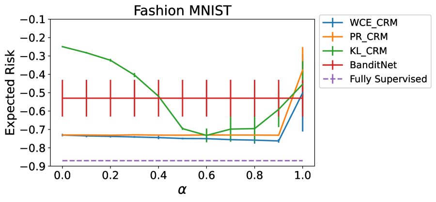
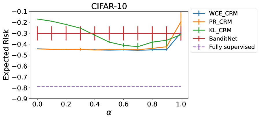
Figure 1: Expected risk of WCE-CRM, PR-CRM and KL-CRM, BandiNet with 10% and supervised approach

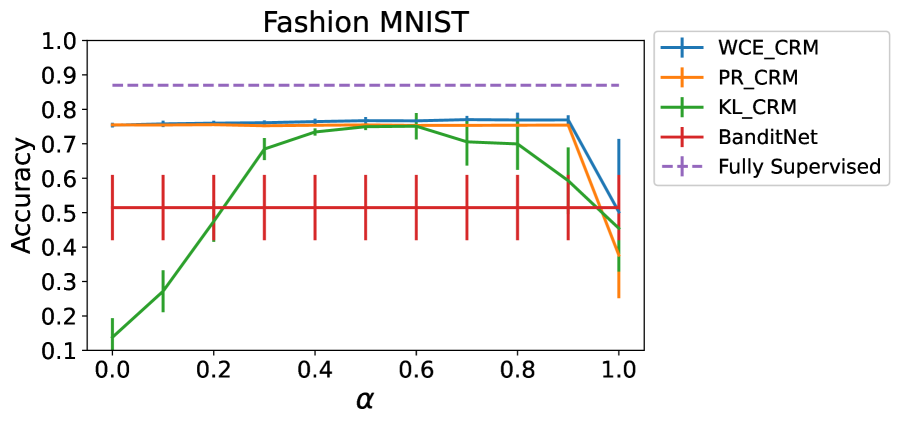
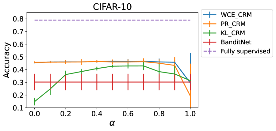
Figure 2: Expected accuracy of WCE-CRM, PR-CRM and KL-CRM, BandiNet with 10% and supervised approach

Note that when $\alpha=0$, all the algorithms use only the logged unknown-reward dataset and when $\alpha=1$, all the algorithms use only the logged known-reward dataset. At $\alpha=0.9$, we achieve the best performance, i.e., $-0.76$, under WCE-CRM, showing the improved performance gained by using the logged unknown-reward dataset. As a second experiment, we ran our WCE-CRM under a scenario where one action is not observed in the logged known-reward dataset; however, we have some samples with respect to this action in the logged unknown-reward dataset. The expected risk for the Fashion-MNIST dataset was -0.75, while the expected risk for CIFAR-10 was -0.44. This result shows that WCE-CRM is robust against unknown actions in the logged known-reward dataset. This result is consistent with the results of Figure 1. Note that in the case of $\alpha=0$ we have an extreme case where the rewards of all actions are missing. Despite this limitation, the information provided with the dataset without rewards leads to positive results. In comparison to BandiNet, which is trained using 10% of the dataset, we also have an improvement. It can be seen that in the case of restricted access to the known-reward dataset, employing the unknown-reward dataset can assist in achieving a better policy. More discussions and experiments on the effect of truncation parameter $\tau$ and also the quality of logging policy are provided in Appendix E.

7 Conclusion and future works

We proposed two new algorithms for Semi-Counterfactual Risk Minimization, including reward-free regularized CRM and Pseudo-reward CRM. The main take-away in reward-free regularized CRM is proposing regularization terms, i.e., KL divergence and reverse KL divergence, independent of reward values, and also the minimization of these terms results in a tighter upper bound on true risk. Likewise, we believe that the idea of KL-CRM and WCE-CRM can be extended to semi-supervised reward learning and using unlabeled data scenarios in reinforcement learning (Konyushkova et al., 2020; Yu et al., 2022). In the pseudo-reward CRM algorithm, we estimated the reward function using the logged known-reward dataset and applied the estimated reward function to samples in the logged unknown-reward dataset to produce the pseudo-rewards and train the model using logged known-reward and pseudo-reward datasets.

The main limitation of this work is the assumption of access to a clean propensity score relating to the probability of an action given a context under the logging policy. We also use propensity scores in both the main objective function and the regularization term. However, we can estimate the propensity score using different methods, e.g., logistic regression (D’Agostino Jr, 1998; Weitzen et al., 2004), generalized boosted models (McCaffrey et al., 2004), neural networks (Setoguchi et al., 2008), or classification and regression trees (Lee et al., 2010, 2011). Therefore, a future line of research is to investigate how different methods of propensity score estimation can be combined with our algorithm to optimize the expected risk using logged known-reward and unknown-reward datasets.

Acknowledgments

The first author, Gholamali Aminian, is supported by the Alan Turing Institute, project code: R-FAIR-001.

A Proofs of Section 4

We first prove the following Lemma:

Lemma 6

Suppose that $f(x)$ is $\sigma$-sub-Gaussian under distribution $P_{X}$. Then, the following upper bound, holds on the difference of expectation of function $f(x)$ respect to two distributions, i.e., $P_{X}$ and $Q_{X}$,

$$|\mathbb{E}_{P_{X}}[f(X)]-\mathbb{E}_{Q_{X}}[f(X)]|\leq\sqrt{2\sigma^{2}D(P_{X}\|Q_{X})}$$ (22)

Proof. From the Donsker-Varadhan representation of KL divergence (Polyanskiy and Wu, 2014), for $\lambda\in\mathbb{R}$ we have:

$$D(P_{X}\|Q_{X}) \geq\mathbb{E}_{P_{X}}[\lambda f(X)]-\log(\mathbb{E}_{Q_{X}}[e^{\lambda f(X)}])$$ (23)

$$\geq\lambda(\mathbb{E}_{P_{X}}[f(X)]-\mathbb{E}_{Q_{X}}[f(X)])-\frac{\lambda^{2}\sigma^{2}}{2}$$ (24)

where (24) is the result of sub-Gaussian assumption. We have:

$$\frac{\lambda^{2}\sigma^{2}}{2}-\lambda(\mathbb{E}_{P_{X}}[f(X)]-\mathbb{E}_{Q_{X}}[f(X)])+D(P_{X}\|Q_{X}) \geq 0$$ (25)

As we have a parabola in $\lambda$ (25) which is positive and it has non-positive discriminant, then the final result holds.

A.1 Proof of Proposition 1

Note that $c_{l}^{2}\leq R^{2}(\pi_{\theta})\leq b_{u}^{2}$ where $c_{l}=\max(c,0)$ and $b_{u}=\max(|c|,b)$.

$$\operatorname{Var}\left(w(A,X)f_{r}(A,X)\right) =\mathbb{E}_{P_{X}\otimes\pi_{0}(A|X)}\left[\left(w(A,X)f_{r}(A,X)\right)^{2}\right]-R^{2}(\pi_{\theta})$$ (26)

$$\leq\mathbb{E}_{P_{X}\otimes\pi_{0}(A|X)}\left[\left(w(A,X)f_{r}(A,X)\right)^{2}\right]-c_{l}^{2}$$ (27)

where $c_{l}=\max(c,0)$. We need to provide an upper bound on $\mathbb{E}_{P_{X}\otimes\pi_{0}(A|X)}\left[\left(w(A,X)f_{r}(A,X)\right)^{2}\right]$. First, we have:

$$\mathbb{E}_{P_{X}\otimes\pi_{0}(A|X)}\left[\left(w(A,X)f_{r}(A,X)\right)^{2}\right] =\mathbb{E}_{P_{X}\otimes\pi_{0}(A|X)}\left[\left(\frac{\pi_{\theta}(A|X)}{\pi_{0}(A|X)}f_{r}(A,X)\right)^{2}\right]$$ (28)

$$=\mathbb{E}_{P_{X}\otimes\pi_{\theta}(A|X)}\left[\frac{\pi_{\theta}(A|X)}{\pi_{0}(A|X)}\left(f_{r}(A,X)\right)^{2}\right]$$ (29)

Using Lemma 6 and assuming sub-Gaussianity under $P_{X}\otimes\pi_{0}(A|X)$ we have:

$$\left|\mathbb{E}_{P_{X}\otimes\pi_{\theta}(A|X)}\left[\frac{\pi_{\theta}(A|X)}{\pi_{0}(A|X)}\left(f_{r}(A,X)\right)^{2}\right]-\mathbb{E}_{P_{X}\otimes\pi_{0}(A|X)}\left[\frac{\pi_{\theta}(A|X)}{\pi_{0}(A|X)}\left(f_{r}(A,X)\right)^{2}\right]\right|\leq$$ (30)

$$\sqrt{2\sigma^{2}D(\pi_{\theta}(A|X)\|\pi_{0}(A|X)|P_{X})},$$

and $f_{r}(A,X)\in[c,b]$, we have:

$$\mathbb{E}_{P_{X}\otimes\pi_{0}(A|X)}\left[\frac{\pi_{\theta}(A|X)}{\pi_{0}(A|X)}\left(f_{r}(A,X)\right)^{2}\right]=\mathbb{E}_{P_{X}\otimes\pi_{\theta}(A|X)}\left[\left(f_{r}(A,X)\right)^{2}\right]\leq b_{u}^{2}$$ (31)

Considering (31) and (30), the following result holds:

$$\mathbb{E}_{P_{X}\otimes\pi_{\theta}(A|X)}\left[\frac{\pi_{\theta}(A|X)}{\pi_{0}(A|X)}\left(f_{r}(A,X)\right)^{2}\right]\leq\sqrt{2\sigma^{2}D(\pi_{\theta}(A|X)\|\pi_{0}(A|X)|P_{X})}+b_{u}^{2},$$ (32)

Using the same approach by assuming sub-Gaussianity under $P_{X}\otimes\pi_{\theta}(A|X)$, we have:

$$\mathbb{E}_{P_{X}\otimes\pi_{\theta}(A|X)}\left[\frac{\pi_{\theta}(A|X)}{\pi_{0}(A|X)}\left(f_{r}(A,X)\right)^{2}\right]\leq\sqrt{2\sigma^{2}D(\pi_{0}(A|X)\|\pi_{\theta}(A|X)|P_{X})}+b_{u}^{2},$$ (33)

And the final result holds by considering (32), (33), $D_{r}(\pi_{\theta}(A|X)\|\pi_{0}(A|X)|P_{X})=D(\pi_{0}(A|X)\|\pi_{\theta}(A|X)|P_{X})$, and (28).

Remark 7

Under Bounded importance weights $\sup_{(x,a)\in\mathcal{X}\times\mathcal{A}}w(a,x)=w_{m}<\infty$, assuming $f_{r}(A,X)\in[c,b]$, and considering $0\leq w(a,x)\leq w_{m}$, then function $w(a,x)f_{r}^{2}(A,X)$ is bounded in $[0,b_{u}^{2}w_{m}]$ where $b_{u}=\max(|c|,b)$, and this function is $\frac{w_{m}b_{u}^{2}}{2}$-sub-Gaussian under any distribution.

A.2 Proof of Proposition 2

Note that $c_{l}^{2}\leq R^{2}(\pi_{\theta})\leq b_{u}^{2}$ where $c_{l}=\max(c,0)$ and $b_{u}=\max(|c|,b)$.

$$\operatorname{Var}\left(w(A,X)f_{r}(A,X)\right) =\mathbb{E}_{P_{X}\otimes\pi_{0}(A|X)}\left[\left(w(A,X)f_{r}(A,X)\right)^{2}\right]-R^{2}(\pi_{\theta})$$ (34)

$$\geq\mathbb{E}_{P_{X}\otimes\pi_{0}(A|X)}\left[\left(w(A,X)f_{r}(A,X)\right)^{2}\right]-b_{u}^{2}$$ (35)

First, we have:

$$\mathbb{E}_{P_{X}\otimes\pi_{0}(A|X)}\left[\left(w(A,X)f_{r}(A,X)\right)^{2}\right] =\mathbb{E}_{P_{X}\otimes\pi_{0}(A|X)}\left[\left(\frac{\pi_{\theta}(A|X)}{\pi_{0}(A|X)}f_{r}(A,X)\right)^{2}\right]$$ (36)

$$=\mathbb{E}_{P_{X}\otimes\pi_{\theta}(A|X)}\left[\frac{\pi_{\theta}(A|X)}{\pi_{0}(A|X)}\left(f_{r}(A,X)\right)^{2}\right]$$ (37)

Considering (37), we provide a lower bound on $\mathbb{E}_{P_{X}\otimes\pi_{\theta}(A|X)}\left[\frac{\pi_{\theta}(A|X)}{\pi_{0}(A|X)}\left(f_{r}(A,X)\right)^{2}\right]$, as follows:

$$\mathbb{E}_{P_{X}\otimes\pi_{\theta}(A|X)}\left[\frac{\pi_{\theta}(A|X)}{\pi_{0}(A|X)}\left(f_{r}(A,X)\right)^{2}\right] =\mathbb{E}_{P_{X}\otimes\pi_{\theta}(A|X)}\left[e^{\log(\frac{\pi_{\theta}(A|X)}{\pi_{0}(A|X)})+2\log(|f_{r}(A,X)|)}\right]$$ (38)

$$\geq e^{\mathbb{E}_{P_{X}\otimes\pi_{\theta}(A|X)}[\log(\frac{\pi_{\theta}(A|X)}{\pi_{0}(A|X)})+2\log(|f_{r}(A,X)|)]}$$ (39)

$$=e^{D(\pi_{\theta}(A|X)\|\pi_{0}(A|X)|P_{X})}(e^{\mathbb{E}_{P_{X}\otimes\pi_{\theta}(A|X)}[\log(|f_{r}(A,X)|)]})^{2}$$ (40)

$$\geq q^{2}e^{D(\pi_{\theta}(A|X)\|\pi_{0}(A|X)|P_{X})},$$ (41)

Where (39) is based on Jensen-inequality for exponential function.

Remark 8

If we consider $f_{r}(a,x)\in[c,b]$ with $b\geq 0$, then we can consider $q=\max(0,c)$.

B Proofs of Section 5

B.1 Proof of Theorem 3

The main idea of the proof is based on (Cortes et al., 2010, Theorem 1). Let us consider $Z=\frac{\pi_{\theta}(A|X)}{\pi_{0}(A|X)}f_{r}(A,X)-R(\pi_{\theta})$ and $|Z|\leq w_{m}$. Now, we have:

$$\operatorname{Var}(Z) =\mathbb{E}_{P_{X}\otimes\pi_{0}(A|X)}\left[\left(\frac{\pi_{\theta}(A|X)}{\pi_{0}(A|X)}f_{r}(A,X)\right)^{2}\right]-R^{2}(\pi_{\theta})$$ (42)

$$\leq w_{m}\sqrt{\frac{\min(D(\pi_{\theta}\|\pi_{0}),D_{r}(\pi_{\theta}\|\pi_{0}))}{2}}+1,$$

where $D(\pi_{\theta}\|\pi_{0})=D(\pi_{\theta}(A|X)\|\pi_{0}(A|X)|P_{X})$ and $D_{r}(\pi_{\theta}\|\pi_{0})=D_{r}(\pi_{\theta}(A|X)\|\pi_{0}(A|X)|P_{X})$. Using Bernstein inequality (Boucheron et al., 2013), we also have:

$$Pr\left(R(\pi_{\theta})-\hat{R}(\pi_{\theta},S)>\epsilon\right)\leq\exp\left(\frac{-n\epsilon^{2}/2}{\operatorname{Var}(Z)+\epsilon w_{m}/3}\right)$$ (43)

Now, setting $\delta=\frac{-n\epsilon^{2}/2}{\operatorname{Var}(Z)+\epsilon w_{m}/3}$ to match the upper bound in (43) and using the variance upper bound (42), the following upper bound with probability at least $(1-\delta)$ holds under $P_{X}\otimes\pi_{0}(A|X)$:

$$R(\pi_{\theta})\leq$$ (44)

$$\quad\hat{R}(\pi_{\theta},S)+\frac{w_{m}\log(\frac{1}{\delta})}{3n}+\sqrt{\frac{w_{m}^{2}\log^{2}(\frac{1}{\delta})}{9n^{2}}+\frac{(w_{m}\sqrt{2\min(D(\pi_{\theta}\|\pi_{0}),D_{r}(\pi_{\theta}\|\pi_{0}))}+2)\log(\frac{1}{\delta})}{n}}$$

By Considering $\sqrt{x+y}\leq\sqrt{x}+\sqrt{y}$, the final result holds.

B.2 Proof of Proposition Prop: estimators

First we have the following decomposition of KL divergence and reverse KL divergence as follows:

$$D(\pi_{\theta}(A|X)\|\pi_{0}(A|X)|P_{X})=\sum_{i=1}^{k}\mathbb{E}_{P_{X}}[(\pi_{\theta}(A=a_{i}|X)\log(\frac{\pi_{\theta}(A=a_{i}|X)}{\pi_{0}(A=a_{i}|X)})]$$ (45)

$$D_{r}(\pi_{\theta}(A|X)\|\pi_{0}(A|X)|P_{X})=\sum_{i=1}^{k}\mathbb{E}_{P_{X}}[\pi_{0}(A=a_{i}|X)\log(\frac{\pi_{0}(A=a_{i}|X)}{\pi_{\theta}(A=a_{i}|X)}]$$ (46)

It suffices to show that:

$$\hat{R}_{\mathrm{KL}}(\pi_{\theta},S_{u})\triangleq\sum_{i=1}^{k}\frac{1}{m_{[i]}}\sum_{(x,a_{i},p)\in S_{u}}\pi_{\theta}(a_{i}|x)\log(\frac{\pi_{\theta}(a_{i}|x)}{p}),$$ (47)

$$\hat{R}_{\mathrm{RKL}}(\pi_{\theta},S_{u})\triangleq\sum_{i=1}^{k}\frac{1}{m_{[i]}}\sum_{(x,a_{i},p)\in S_{u}}-p\log(\pi_{\theta}(a_{i}|x))+p\log(p),$$ (48)

As we assume KL divergence and reverse KL divergence are bounded, then we have $\mathbb{E}_{P_{X}}[\pi_{0}(a_{i}|X)\log(\frac{\pi_{0}(a_{i}|X)}{\pi_{\theta}(a_{i}|X)})]$ and $\mathbb{E}_{P_{X}}[\pi_{\theta}(a_{i}|x)\log(\frac{\pi_{\theta}(a_{i}|x)}{\pi_{0}(a_{i}|x)})]$ $\forall i\in[k]$ exist and they are bounded. Now, by considering Law of Large number Hsu and Robbins (1947), we have that:

$$\frac{1}{m_{[i]}}\sum_{(x,a_{i},p)\in S_{u}}\pi_{0}(a_{i}|x)\log(\frac{\pi_{0}(a_{i}|x)}{\pi_{\theta}(a_{i}|x)})\xrightarrow{m_{[i]}\rightarrow\infty}\mathbb{E}_{P_{X}}[\pi_{0}(a_{i}|X)\log(\frac{\pi_{0}(a_{i}|X)}{\pi_{\theta}(a_{i}|X)})],$$ (49)

and

$$\frac{1}{m_{[i]}}\sum_{(x,a_{i},p)\in S_{u}}\pi_{\theta}(a_{i}|x)\log(\frac{\pi_{\theta}(a_{i}|x)}{\pi_{0}(a_{i}|x)})\xrightarrow{m_{[i]}\rightarrow\infty}\mathbb{E}_{P_{X}}[\pi_{\theta}(a_{i}|x)\log(\frac{\pi_{\theta}(a_{i}|x)}{\pi_{0}(a_{i}|x)})].$$ (50)

By considering (47), (48) and $m_{[i]}\rightarrow\infty$, $\forall i\in[k]$, the final results hold.

B.3 Proof of Proposition 5

We have:

$$R(\pi_{\theta}) =\mathbb{E}_{P_{X}}[\mathbb{E}_{\pi_{\theta}(A|X)}[f_{r}(X,A)]].$$ (51)

$$R(\pi_{0}) =\mathbb{E}_{P_{X}}[\mathbb{E}_{\pi_{0}(A|X)}[f_{r}(X,A)]].$$ (52)

As the reward function is bounded in $[-1,0]$, then it is $\frac{1}{2}$-sub-Gaussian under all distributions. Now, by considering Lemma 6, the final result holds.

C Proposition 1 Comparison

Without loss of generality, let us consider $f_{r}(a,x)\in[-1,0]$. Then, we have $\sigma=\frac{w_{m}}{2}$, $b_{u}=1$ and $c_{l}=0$ in Proposition 1. The upper bound in Proposition 1 for $\sup_{(x,a)\in\mathcal{X}\times\mathcal{A}}\frac{\pi_{(}a|x)}{\pi_{0}(a|x)}=w_{m}<\infty$ and considering the KL divergence between $\pi_{\theta}$ and $\pi_{0}$ is as follows:

$$\mathbb{E}_{P_{X}\otimes\pi_{0}(A|X)}\left[\left(\frac{\pi_{\theta}(A|X)}{\pi_{0}(A|X)}f_{r}(A,X)\right)^{2}\right]\leq w_{m}\sqrt{\frac{D(\pi_{\theta}(A|X)\|\pi_{0}(A|X)|P_{X})}{2}}+1,$$ (53)

And the upper bound on second moment of importance weighted reward function in (Cortes et al., 2010, Lemma 1) is as follows:

$$\mathbb{E}_{P_{X}\otimes\pi_{0}(A|X)}\left[\left(\frac{\pi_{\theta}(A|X)}{\pi_{0}(A|X)}f_{r}(A,X)\right)^{2}\right]\leq\chi^{2}(\pi_{\theta}(A|X)\|\pi_{0}(A|X)|P_{X})+1$$ (54)

It can be shown that $\chi^{2}(\pi_{\theta}(A|X)\|\pi_{0}(A|X)|P_{X})\leq w_{m}$. It is shown by Sason and Verdú (2016) that:

$$D(\pi_{\theta}(A|X)\|\pi_{0}(A|X)|P_{X})\leq\log(\chi^{2}(\pi_{\theta}(A|X)\|\pi_{0}(A|X)|P_{X})+1)$$ (55)

Using (55) in (53) and comparing to (54), then for $w_{m}<e^{2}-1$, $\exists C\in[0,w_{m}]$, e.g. if $w_{m}=2$ we have $C\approx 1.28$, where if $\chi^{2}(\pi_{\theta}(A|X)\|\pi_{0}(A|X)|P_{X})\geq C$, then we have:

$$\log(\chi^{2}(\pi_{\theta}(A|X)\|\pi_{0}(A|X)|P_{X})+1)\leq\frac{2(\chi^{2}(\pi_{\theta}(A|X)\|\pi_{0}(A|X)|P_{X}))^{2}}{w_{m}^{2}}$$ (56)

Therefore, the upper bound on the variance given in Proposition 1 is tighter than that of (Cortes et al., 2010, Lemma 1) for $\chi^{2}(\pi_{\theta}(A|X)\|\pi_{0}(A|X)|P_{X})\geq C$ if $w_{m}<e^{2}-1$ and $C$ is the solution of $\log(1+x)-2x^{2}/w_{m}^{2}=0$.

D Semi-CRM via Pseudo-rewards

The PR-CRM algorithm is proposed in Algorithm 2.

Data: $S=(x_{i},a_{i},p_{i},r_{i})_{i=1}^{n}$ sampled from $\pi_{0}$, $S_{u}=(x_{j},a_{j},p_{j})_{j=1}^{m}$ sampled from $\pi_{0}$, hyper-parameters $\zeta$ and $\tau$, initial policy $\pi_{\theta^{0}}(a|x)$, and max epochs for the whole algorithm $M$

Result: An optimized neural network $\pi^{\star}_{\theta}(a|x)$ which minimize the risk

while epoch $\leq M$ do

       Sample $n$ real samples $(x_{j},a_{j},p_{j},r_{j})$ from $S$

       Estimate $\hat{f}_{r}(x,a)$ using the regression with weighted squared loss function: $\frac{1}{\mathrm{P}}\sum_{i=1}^{n}p_{i}(r_{i}-\hat{f}_{r}(x_{i},a_{i}))^{2}$

end while

for $i=1,\cdots,m$ do

      Sample $(x_{i},a_{i},p_{i})$ from $S_{u}$

       Produce the pseudo-reward $\hat{r}_{i}=\hat{f}_{r}(x_{i},a_{i})$

end for

while epoch $\leq M$ do

       Sample $m_{1}$ samples $(x_{i},a_{i},p_{i},\hat{r}_{i})$ and $n_{1}$ samples $(x_{j},a_{j},p_{j},r_{j})$ from $S_{u}$ and $S$, resp.

       Estimate the re-weighted loss as

$$\hat{R}^{\tau,\zeta}(\theta^{t_{g}}) =\frac{\alpha}{n_{1}+m_{1}}\left(\sum_{i=1}^{n_{1}}r_{i}\frac{\pi_{\theta^{t_{g}}}(a_{i}|x_{i})}{\max(\zeta,p_{i})}+\sum_{j=1}^{m_{1}}\hat{r}_{j}\frac{\pi_{\theta^{t_{g}}}(a_{j}|x_{j})}{\max(\zeta,p_{j})}\right)$$

$$\quad+(1-\alpha)\sum_{i=1}^{k}\frac{-1}{m_{[i]}}\sum_{(x,a_{i},p)\in S_{u}\cup S}\max(\tau,p)\log(\pi_{\theta^{t_{g}}}(a_{i}|x))$$

       Get the gradient as $g_{1}\leftarrow\nabla_{\theta^{t_{g}}}\hat{R}(\theta^{t_{g}})$

       Update $\theta^{t_{g}+1}=\theta^{t_{g}}-g_{1}$

end while

Algorithm 2 PR-CRM Algorithm

E Experiments

We compare the best performance of all algorithms in Table 1.

Table 1: Comparison of different algorithms for Fashion-MNIST (FMNIST) and CIFAR-10 by considering standard deviation.

	WCE-CRM	KL-CRM	PR-CRM
Expected Risk (FMNIST)	$-\bm{0.76\pm 0.003}$	$-0.72\pm 0.033$	$-0.75\pm 0.021$
Accuracy (FMNIST)	$\bm{0.77\pm 0.005}$	$0.74\pm 0.004$	$0.76\pm 0.009$
Expected Risk (CIFAR-10)	$-0.45\pm 0.005$	$-0.41\pm 0.034$	$-\bm{0.45\pm 0.003}$
Accuracy (CIFAR-10)	$0.46\pm 0.005$	$0.43\pm 0.011$	$\bm{0.46\pm 0.004}$

For comparison purposes, we estimated the expected risk of the logging policy in both datasets. The expected risk of the Fashion MNIST dataset under the logging policy is $-\bm{0.71}$, while the expected risk for the CIFAR-10 dataset was $-\bm{0.42}$. The results show that our algorithms can achieve a better policy compared to the logging policy in different scenarios.

The boost in performance depends on the quality of the logging policy on the first place. Figure 3(a) shows the expected risk as a function of the percentage of the training set used to learn the logging policy. Note that more data leads to a better logging policy, i.e., better training loss, which in turn leads to a lower expected risk. We also study the effect of the truncation parameter for propensity scores belongs to logged unknown-reward dataset, i.e. $\tau$ in Figure 3(b). As we increase the $\tau$ value, we reduce the effect of noise in propensity scores. Note that, in general, higher values of $\tau$ lead to a lower expected risk. For example, in $\tau=1$, we do not consider propensity score. A second important remark is that the WCE-CRM is much more stable than the KL-CRM, as shown by the error bars in Figures 3(a) and 3(b) (which represent the standard deviation over the 10 runs). We

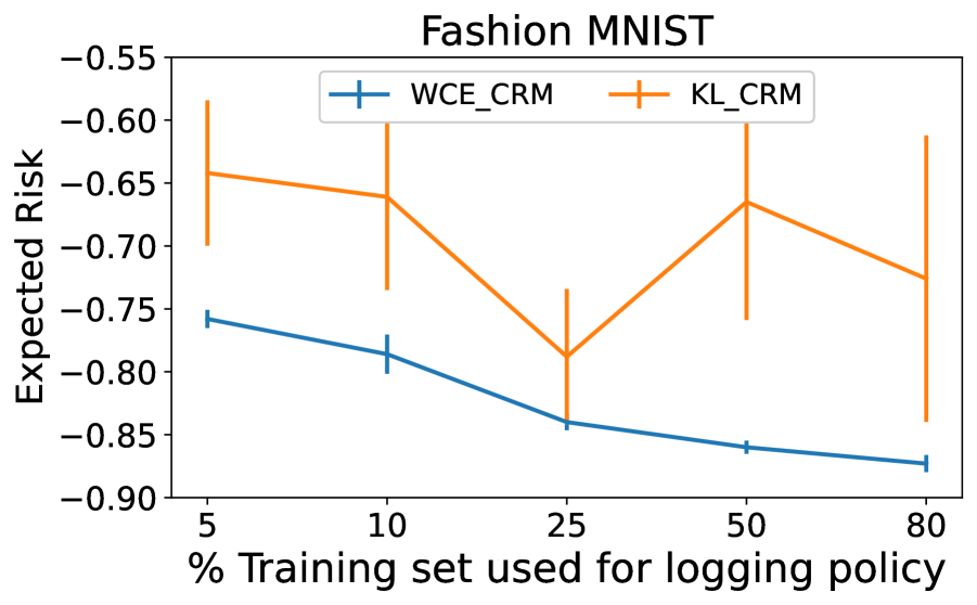
(a) Effect of the logging policy

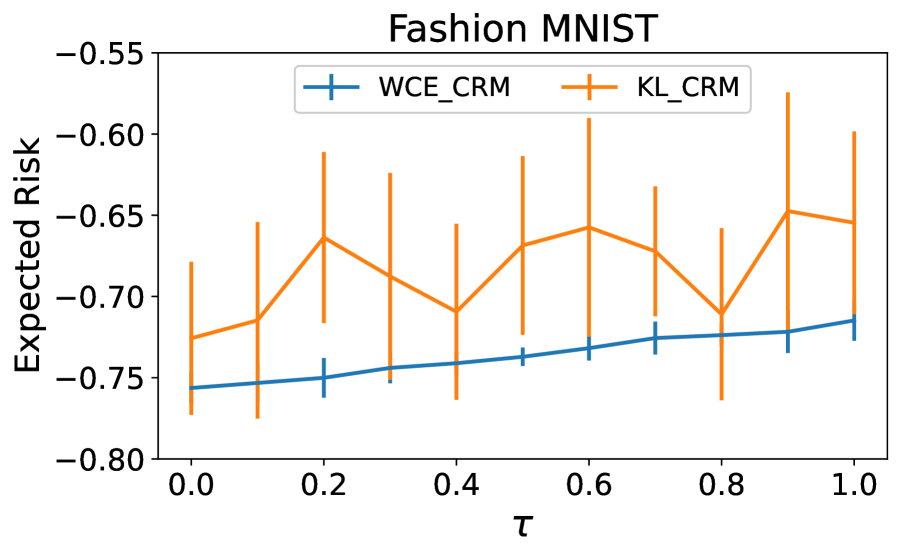
(b) Effect of $\tau$

Figure 3: Effect of the hyper-parameter $\tau$ and the number of instances used to learn the logging policy on the expected risk.

F Code details

The supplementary material includes a zip file named CODE_CRM.zip with the following files:

• requirements.txt: It contains the python libraries required to reproduce our results.

• CRM_Lib: A folder containing an in-house developed library with the algorithms described in the main manuscript, as well as helper functions that were used during our experiments.

• Algorithm_Comparison.ipynb A jupyter notebook that has the code needed to reproduce the experiments described in the main manuscript.

• Classification_2_Bandit.ipynb This jupyter notebook contains the code to transform the Fashion MNIST dataset to a Bandit datset.

• Classification_2_Bandit-CIFAR-10.ipynb This jupyter notebook contains the code to transform the CIFAR-10 dataset to a Bandit datset.

To use this code, the user needs to first download the CIFAR-10 dataset from https://www.cs.toronto.edu/ kriz/cifar.html and make sure that the the folder cifar-10-batches-py is inside the folder CODE_CRM. Then, the user needs to install the python libraries included in the file requirements.txt. After that, the user needs to run the jupyter notebooks Classification_2_Bandit.ipynb and Classification_2_Bandit-CIFAR-10.ipynb. Finally, the user should run the jupyter notebook Algorithm_Comparison.ipynb. There, the user might modify the different parameters and settings of the experiments.

All our experiments were run using the Google Cloud Platform, using a virtual computer with 4 N1-vCPU and 10 GB of RAM.

G True Risk Regularization

In this section, we study the true risk regularization using KL divergence between target and logging policy, i.e., $D(\pi_{\theta}(A|X)\|\pi_{0}(A|X)|P_{X})$, as follows:

$$\min_{\pi_{\theta}}\alpha R(\pi_{\theta})+(1-\alpha)D(\pi_{\theta}(A|X)\|\pi_{0}(A|X)|P_{X}),\quad\alpha\in[0,1]$$ (57)

It is possible to provide the the optimal solution to regularized minimization (57).

Theorem 9

Considering the true risk minimization with KL divergence regularization,

$$\min_{\pi_{\theta}}\alpha R(\pi_{\theta})+(1-\alpha)D(\pi_{\theta}(A|X)\|\pi_{0}(A|X)|P_{X}),\quad\alpha\in(0,1],$$ (58)

the optimal target policy is:

$$\pi_{\theta}^{\star}(A=a|X=x)=\frac{\pi_{0}(A=a|X=x)e^{-\frac{\alpha}{(1-\alpha)}f_{r}(a,x)}}{\mathbb{E}_{\pi_{0}}[e^{-\frac{\alpha}{(1-\alpha)}f_{r}(a,x)}]}$$ (59)

Proof  The minimization problem (57) can be written as follows:

$$\min_{\pi_{\theta}}\mathbb{E}_{P_{X}}[\mathbb{E}_{\pi_{\theta}(A|X)}[f_{r}(A,X)]]+\frac{(1-\alpha)}{\alpha}D(\pi_{\theta}(A|X)\|\pi_{0}(A|X)|P_{X}),\quad\alpha\in(0,1]$$ (60)

Using the same approach by Zhang (2006); Aminian et al. (2021) and considering $\frac{\alpha}{(1-\alpha)}$ as the inverse temperature, the final result holds.  
The optimal target policy under KL divergence regularization, i.e.,

$$\pi_{\theta}^{\star}(A=a|X=x)=\frac{\pi_{0}(A=a|X=x)e^{-\frac{\alpha}{(1-\alpha)}f_{r}(a,x)}}{\mathbb{E}_{\pi_{0}}[e^{-\frac{\alpha}{(1-\alpha)}f_{r}(a,x)}]}$$ (61)

provide the following insights:

• The optimal target policy, $\pi_{\theta}^{\star}(A|X)$, is a stochastic policy similar to the Softmax policy.

• The optimal target policy is invariant with respect to constant shift in the reward function.

• For asymptotic condition, i.e., $\alpha\rightarrow 1$, the optimal target policy will be deterministic policy.

• We can choose the KL divergence instead of square root of KL divergence as a regularizer for IPS estimator minimization.

References

- Abbeel and Ng (2004) Pieter Abbeel and Andrew Y Ng. Apprenticeship learning via inverse reinforcement learning. In Proceedings of the twenty-first international conference on Machine learning, page 1, 2004.
- Aggarwal et al. (2016) Charu C Aggarwal et al. Recommender systems, volume 1. Springer, 2016.
- Alaa and van der Schaar (2017) Ahmed M Alaa and Mihaela van der Schaar. Bayesian inference of individualized treatment effects using multi-task gaussian processes. Advances in Neural Information Processing Systems, 30, 2017.
- Aminian et al. (2021) Gholamali Aminian, Yuheng Bu, Laura Toni, Miguel Rodrigues, and Gregory Wornell. An exact characterization of the generalization error for the gibbs algorithm. Advances in Neural Information Processing Systems, 34:8106–8118, 2021.
- Aminian et al. (2022) Gholamali Aminian, Mahed Abroshan, Mohammad Mahdi Khalili, Laura Toni, and Miguel RD Rodrigues. An information-theoretical approach to semi-supervised learning under covariate-shift. AISTATS, 2022.
- Atan et al. (2018) Onur Atan, William R Zame, and Mihaela Van Der Schaar. Counterfactual policy optimization using domain-adversarial neural networks. In ICML CausalML workshop, 2018.
- Bertsimas et al. (2017) Dimitris Bertsimas, Nathan Kallus, Alexander M Weinstein, and Ying Daisy Zhuo. Personalized diabetes management using electronic medical records. Diabetes care, 40(2):210–217, 2017.
- Beygelzimer and Langford (2009) Alina Beygelzimer and John Langford. The offset tree for learning with partial labels. In Proceedings of the 15th ACM SIGKDD international conference on Knowledge discovery and data mining, pages 129–138, 2009.
- Bottou et al. (2013) Léon Bottou, Jonas Peters, Joaquin Quiñonero-Candela, Denis X Charles, D Max Chickering, Elon Portugaly, Dipankar Ray, Patrice Simard, and Ed Snelson. Counterfactual reasoning and learning systems: The example of computational advertising. Journal of Machine Learning Research, 14(11), 2013.
- Boucheron et al. (2013) Stéphane Boucheron, Gábor Lugosi, and Pascal Massart. Concentration inequalities: A nonasymptotic theory of independence. Oxford university press, 2013.
- Cao et al. (2021) Haoyang Cao, Samuel Cohen, and Lukasz Szpruch. Identifiability in inverse reinforcement learning. Advances in Neural Information Processing Systems, 34, 2021.
- Cleveland and Devlin (1988) William S Cleveland and Susan J Devlin. Locally weighted regression: an approach to regression analysis by local fitting. Journal of the American statistical association, 83(403):596–610, 1988.
- Cortes et al. (2010) Corinna Cortes, Yishay Mansour, and Mehryar Mohri. Learning bounds for importance weighting. In Nips, volume 10, pages 442–450. Citeseer, 2010.
- Csiszár and Körner (2011) Imre Csiszár and János Körner. Information Theory: Coding Theorems for Discrete Memoryless Systems. Cambridge University Press, 2011.
- D’Agostino Jr (1998) Ralph B D’Agostino Jr. Propensity score methods for bias reduction in the comparison of a treatment to a non-randomized control group. Statistics in medicine, 17(19):2265–2281, 1998.
- Dudík et al. (2014) Miroslav Dudík, Dumitru Erhan, John Langford, and Lihong Li. Doubly robust policy evaluation and optimization. Statistical Science, 29(4):485–511, 2014.
- Faury et al. (2020) Louis Faury, Ugo Tanielian, Elvis Dohmatob, Elena Smirnova, and Flavian Vasile. Distributionally robust counterfactual risk minimization. In Proceedings of the AAAI Conference on Artificial Intelligence, volume 34, pages 3850–3857, 2020.
- Finn et al. (2016) Chelsea Finn, Sergey Levine, and Pieter Abbeel. Guided cost learning: Deep inverse optimal control via policy optimization. In International conference on machine learning, pages 49–58. PMLR, 2016.
- Gao et al. (2022) Ruijiang Gao, Max Biggs, Wei Sun, and Ligong Han. Enhancing counterfactual classification via self-training. Proceedings of the AAAI conference on artificial intelligence, 2022.
- Grandvalet et al. (2005) Yves Grandvalet, Yoshua Bengio, et al. Semi-supervised learning by entropy minimization. CAP, 367:281–296, 2005.
- He et al. (2021) Haiyun He, Hanshu Yan, and Vincent YF Tan. Information-theoretic generalization bounds for iterative semi-supervised learning. arXiv preprint arXiv:2110.00926, 2021.
- Hsu and Robbins (1947) Pao-Lu Hsu and Herbert Robbins. Complete convergence and the law of large numbers. Proceedings of the National Academy of Sciences of the United States of America, 33(2):25, 1947.
- Ionides (2008) Edward L Ionides. Truncated importance sampling. Journal of Computational and Graphical Statistics, 17(2):295–311, 2008.
- Jang et al. (2016) Eric Jang, Shixiang Gu, and Ben Poole. Categorical reparameterization with gumbel-softmax. arXiv preprint arXiv:1611.01144, 2016.
- Joachims et al. (2018) Thorsten Joachims, Adith Swaminathan, and Maarten de Rijke. Deep learning with logged bandit feedback. In International Conference on Learning Representations, 2018.
- Johansson et al. (2016) Fredrik Johansson, Uri Shalit, and David Sontag. Learning representations for counterfactual inference. In International conference on machine learning, pages 3020–3029. PMLR, 2016.
- Kallus (2018) Nathan Kallus. Balanced policy evaluation and learning. Advances in neural information processing systems, 31, 2018.
- Konyushkova et al. (2020) Ksenia Konyushkova, Konrad Zolna, Yusuf Aytar, Alexander Novikov, Scott Reed, Serkan Cabi, and Nando de Freitas. Semi-supervised reward learning for offline reinforcement learning. arXiv preprint arXiv:2012.06899, 2020.
- Kosorok and Laber (2019) Michael R Kosorok and Eric B Laber. Precision medicine. Annual review of statistics and its application, 6:263–286, 2019.
- Krizhevsky et al. (2009) Alex Krizhevsky, Geoffrey Hinton, et al. Learning multiple layers of features from tiny images. 2009.
- Kuzborskij et al. (2021) Ilja Kuzborskij, Claire Vernade, Andras Gyorgy, and Csaba Szepesvári. Confident off-policy evaluation and selection through self-normalized importance weighting. In International Conference on Artificial Intelligence and Statistics, pages 640–648. PMLR, 2021.
- Langford et al. (2008) John Langford, Alexander Strehl, and Jennifer Wortman. Exploration scavenging. In Proceedings of the 25th international conference on Machine learning, pages 528–535, 2008.
- Lee et al. (2010) Brian K Lee, Justin Lessler, and Elizabeth A Stuart. Improving propensity score weighting using machine learning. Statistics in medicine, 29(3):337–346, 2010.
- Lee et al. (2011) Brian K Lee, Justin Lessler, and Elizabeth A Stuart. Weight trimming and propensity score weighting. PloS one, 6(3):e18174, 2011.
- Lee et al. (2013) Dong-Hyun Lee et al. Pseudo-label: The simple and efficient semi-supervised learning method for deep neural networks. In Workshop on Challenges in Representation Learning, ICML, 2013.
- Li et al. (2011) Lihong Li, Wei Chu, John Langford, and Xuanhui Wang. Unbiased offline evaluation of contextual-bandit-based news article recommendation algorithms. In Proceedings of the fourth ACM international conference on Web search and data mining, pages 297–306, 2011.
- London and Sandler (2018) Ben London and Ted Sandler. Bayesian counterfactual risk minimization. arXiv:1806.11500, 2018.
- Maurer and Pontil (2009) Andreas Maurer and Massimiliano Pontil. Empirical bernstein bounds and sample variance penalization. In Proceedings of the 22nd Conference on Learning Theory, (COLT) 2009., 2009.
- McCaffrey et al. (2004) Daniel F McCaffrey, Greg Ridgeway, and Andrew R Morral. Propensity score estimation with boosted regression for evaluating causal effects in observational studies. Psychological methods, 9(4):403, 2004.
- Papini et al. (2019) Matteo Papini, Alberto Maria Metelli, Lorenzo Lupo, and Marcello Restelli. Optimistic policy optimization via multiple importance sampling. In International Conference on Machine Learning, pages 4989–4999. PMLR, 2019.
- Polyanskiy and Wu (2014) Yury Polyanskiy and Yihong Wu. Lecture notes on information theory. Lecture Notes for ECE563 (UIUC) and, 6(2012-2016):7, 2014.
- Rosenbaum and Rubin (1983) Paul R Rosenbaum and Donald B Rubin. The central role of the propensity score in observational studies for causal effects. Biometrika, 70(1):41–55, 1983.
- Sason and Verdú (2016) Igal Sason and Sergio Verdú. -divergence inequalities. IEEE Transactions on Information Theory, 62(11):5973–6006, 2016.
- Schulman et al. (2015) John Schulman, Sergey Levine, Pieter Abbeel, Michael Jordan, and Philipp Moritz. Trust region policy optimization. In International conference on machine learning, pages 1889–1897. PMLR, 2015.
- Setoguchi et al. (2008) Soko Setoguchi, Sebastian Schneeweiss, M Alan Brookhart, Robert J Glynn, and E Francis Cook. Evaluating uses of data mining techniques in propensity score estimation: a simulation study. Pharmacoepidemiology and drug safety, 17(6):546–555, 2008.
- Shalit et al. (2017) Uri Shalit, Fredrik D Johansson, and David Sontag. Estimating individual treatment effect: generalization bounds and algorithms. In International Conference on Machine Learning, pages 3076–3085. PMLR, 2017.
- Simonyan and Zisserman (2014) Karen Simonyan and Andrew Zisserman. Very deep convolutional networks for large-scale image recognition. arXiv preprint arXiv:1409.1556, 2014.
- Strehl et al. (2010) Alex Strehl, John Langford, Lihong Li, and Sham M Kakade. Learning from logged implicit exploration data. Advances in neural information processing systems, 23, 2010.
- Sugiyama et al. (2007) Masashi Sugiyama, Shinichi Nakajima, Hisashi Kashima, Paul Buenau, and Motoaki Kawanabe. Direct importance estimation with model selection and its application to covariate shift adaptation. Advances in neural information processing systems, 20, 2007.
- Swaminathan and Joachims (2015a) Adith Swaminathan and Thorsten Joachims. Batch learning from logged bandit feedback through counterfactual risk minimization. The Journal of Machine Learning Research, 16(1):1731–1755, 2015a.
- Swaminathan and Joachims (2015b) Adith Swaminathan and Thorsten Joachims. The self-normalized estimator for counterfactual learning. advances in neural information processing systems, 28, 2015b.
- Tang et al. (2013) Liang Tang, Romer Rosales, Ajit Singh, and Deepak Agarwal. Automatic ad format selection via contextual bandits. In Proceedings of the 22nd ACM international conference on Information & Knowledge Management, pages 1587–1594, 2013.
- Thomas et al. (2015) Philip Thomas, Georgios Theocharous, and Mohammad Ghavamzadeh. High-confidence off-policy evaluation. In Proceedings of the AAAI Conference on Artificial Intelligence, 2015.
- Weitzen et al. (2004) Sherry Weitzen, Kate L Lapane, Alicia Y Toledano, Anne L Hume, and Vincent Mor. Principles for modeling propensity scores in medical research: a systematic literature review. Pharmacoepidemiology and drug safety, 13(12):841–853, 2004.
- Wu and Wang (2018) Hang Wu and May Wang. Variance regularized counterfactual risk minimization via variational divergence minimization. In International Conference on Machine Learning, pages 5353–5362. PMLR, 2018.
- Xiao et al. (2017) Han Xiao, Kashif Rasul, and Roland Vollgraf. Fashion-mnist: a novel image dataset for benchmarking machine learning algorithms, 2017.
- Xie et al. (2018) Yuan Xie, Boyi Liu, Qiang Liu, Zhaoran Wang, Yuan Zhou, and Jian Peng. Off-policy evaluation and learning from logged bandit feedback: Error reduction via surrogate policy. In International Conference on Learning Representations, 2018.
- Yang et al. (2021) Xiangli Yang, Zixing Song, Irwin King, and Zenglin Xu. A survey on deep semi-supervised learning. arXiv preprint arXiv:2103.00550, 2021.
- Yu et al. (2022) Tianhe Yu, Aviral Kumar, Yevgen Chebotar, Karol Hausman, Chelsea Finn, and Sergey Levine. How to leverage unlabeled data in offline reinforcement learning. arXiv preprint arXiv:2202.01741, 2022.
- Zhang (2006) Tong Zhang. Information-theoretic upper and lower bounds for statistical estimation. IEEE Transactions on Information Theory, 52(4):1307–1321, 2006.