Lax Operator and superspin chains from
 4D CS gauge theory

Abstract

We study the properties of interacting line defects in the four-dimensional Chern Simons (CS) gauge theory with invariance given by the $SL\left(m|n\right)$ super-group family. From this theory, we derive the oscillator realisation of the Lax operator for superspin chains with $SL(m|n)$ symmetry. To this end, we investigate the holomorphic property of the bosonic Lax operator $\mathcal{L}$ and build a differential equation $\mathfrak{D}\mathcal{L}=0$ solved by the Costello-Gaioto-Yagi realisation of $\mathcal{L}$ in the framework of the CS theory. We generalize this construction to the case of gauge super-groups, and develop a Dynkin super-diagram algorithm to deal with the decomposition of the Lie superalgebras. We obtain the generalisation of the Lax operator describing the interaction between the electric Wilson super-lines and the magnetic ’t Hooft super-defects. This coupling is given in terms of a mixture of bosonic and fermionic oscillator degrees of freedom in the phase space of magnetically charged ’t Hooft super-lines. The purely fermionic realisation of the superspin chain Lax operator is also investigated and it is found to coincide exactly with the $\mathbb{Z}_{2}$- gradation of Lie superalgebras. 
Keywords: 4D Chern-Simons theory, Super-gauge symmetry, Lie superalgebras and Dynkin super-diagrams, Superspin chains and integrability, Super- Lax operator.

1 Introduction

Four-dimensional Chern-Simons theory living on $\mathbb{R}^{2}\times C$ is a topological gauge field theory with a complexified gauge symmetry $G$ [1]. Its basic observables are given by line and surface defects such as the electrically charged Wilson lines and the magnetically charged ’t Hooft lines [1, 2, 3, 4, 5, 6, 7]. These lines expand in the topological plane $\mathbb{R}^{2}$ and are located at a point $z$ of the complex holomorphic line $C$. The Chern-Simons (CS) gauge theory offers a powerful framework to study the Yang-Baxter equation (YBE) of integrable 2D systems [1, 8, 9, 10, 11, 12] and statistical mechanics of quantum spin chains [13, 14, 15, 16, 17, 18, 19, 20]. This connection between the two research areas is sometimes termed as the Gauge/YBE correspondence [21, 22]. In these regards, the topological invariance of the crossings of three Wilson lines in the 4D theory, which can be interpreted as interactions between three particle states, yields a beautiful graphic realisation of the YBE. Meanwhile, the R-matrix is represented by the crossing of two Wilson lines and is nicely calculated in the 4D CS gauge theory using the Feynman diagram method [1, 8, 23, 24].

In the same spirit, a quantum integrable XXX spin chain of $N$ nodes can be generated in the CS gauge theory by taking $N$ electrically charged Wilson lines located at a point $z$ of $C$ [14, 13]. These parallel lines are aligned along a direction of $\mathbb{R}^{2}$ and are simultaneously crossed by a perpendicular magnetic ’t Hooft line at $z^{\prime}\neq z$. The ’t Hooft line defect plays an important role in this modeling as it was interpreted in terms of the transfer (monodromy) matrix [3, 5, 25] and the Q-operators of the spin chain [13, 26, 27]. In this setup, the nodes’ spin states of the quantum chain are identified with the weight states of the Wilson lines, which in addition to the spectral parameter $z$, are characterised by highest weight representations $\boldsymbol{R}$ of the gauge symmetry $G$ [7]. Moreover, to every crossing vertex, corresponding to a node of the spin chain, is associated a Lax operator (L-operator) describing the Wilson-’t Hooft lines’ coupling. Thus, the RLL equations of the spin chain integrability can be graphically represented following the YBE/Gauge correspondence by the crossings of two Wilson lines with a ’t Hooft line and with each other.

In this paper, we investigate the integrability of superspin chains in the framework of the 4D CS theory with gauge super-groups while focussing on the $SL(m|n)$ family. On the chain side, the superspin states are as formulated in [29] with values in the fundamental representation of $SL(m|n)$. On the gauge theory side, the superspin chain is described by $N$ Wilson super-lines crossed by a ’t Hooft super-line charged under $SL(m|n)$. These super-lines are graded extensions of the bosonic ones of the CS theory; they are described in sub-subsection 5.1.2; in particular eqs(5.27)-(5.29) and the Figures 3, 4. To that purpose, we develop the study of the extension of the standard CS theory to the case of classical gauge super-groups as well as the implementation of the super-line defects and their interactions. We begin by revisiting the construction of the L-operator in the CS theory with bosonic gauge symmetry and explicitize the derivation of the parallel transport of the gauge fields in the presence of ’t Hooft line defects with Dirac-like singularity following [13]. We also build the differential Lax equation, solved by the oscillator realisation of the L-operator, and use it to motivate its extension to supergroups. Then, we describe useful aspects concerning Lie superalgebras and their representations; and propose a diagrammatic algorithm to approach the construction of the degenerate L-operators for every node of the $sl(m|n)$ spin chain. This description has been dictated by: $\left(i\right)$ the absence of a generalised Levi-theorem for superalgebras’ decomposition [30, 31] and $\left(ii\right)$ the multiplicity of Dynkin Super-Diagrams (DSD) associated to a given superalgebra underlying the gauge supergroup symmetry. Next, we describe the basics of the CS theory with $SL(m|n)$ gauge invariance. We focus on the distinguished $sl(m|n)$ superalgebras characterized by a minimal number of fermionic nodes in the DSDs and provide new results concerning the explicit calculation of the super- Lax operators from the gauge theory in consideration. These super L-operators are given in terms of a mixed system of bosonic and fermionic oscillators that we study in details. On one hand, these results contribute to understand better the behaviour of the super- gauge fields in the presence of ’t Hooft lines acting like magnetic Dirac monopoles. On the other hand, we recover explicit results from the literature of integrable superspin chains. This finding extends the consistency of the Gauge/YBE correspondence to supergroups and opens the door for other links to supersymmetric quiver gauge theories and D-brane systems of type II string theory and M2/M5-brane systems of M-theory  [32, 33, 34].

The organisation is as follows. In section 2, we recall basic features of the topological 4D Chern Simons theory with bosonic gauge symmetry $G$. We describe the moduli space of solutions to the equations of motion in the presence of interacting Wilson and ’t Hooft lines and show how the Dirac singularity properties of the magnetic ’t Hooft line lead to an exact description of the oscillator Lax operator for XXX spin chains with bosonic symmetry. In section 3, we derive the differential equation $\mathcal{D}L=0$ verified by the CGY formula $e^{X}z^{\mu}e^{Y}$ [13] for the oscillator realisation of the L-operator. We rely on the fact that this formula is based on the Levi- decomposition of Lie algebras which means that $L(z)$ is a function of the three quantities $\left(\mu,X,Y\right)$ obeying an $sl\left(2\right)$ algebra. We also link this equation to the usual time evolution equation of the Lax operator. Then, we assume that this characterizing behaviour of $L(z)$ described by the differential equation is also valid for superalgebras and use this assumption to treat CS theory with a super- gauge invariance. For illustration, we study the example of the $GL\left(1|1\right)$ theory as a simple graded extension of the $GL(2)$ case. In section 4, we investigate the CS theory for the case of gauge supergroups and describe the useful mathematical tools needed for this study, in particular, the issue regarding the non uniqueness of the DSDs. In section 5, we provide the fundamental building blocks of the CS with $SL\left(m|n\right)$ gauge invariance ($m\neq n$) and define its basic elements that we will need to generalise the expression of the oscillator Lax operator in the super- gauge theory. Here, the distinguished superalgebra is decomposed by cutting a node of the DSD in analogy to the Levi- decomposition of Lie algebras. In section 6, we build the super L-operator associated to $SL\left(m|n\right)$ and explicit the associated bosonic and fermionic oscillator degrees of freedom. We also specify the special pure fermionic case where the Lax operator of the superspin chain is described by fermionic harmonic oscillators. Section 7 is devoted to conclusions and comments. Three appendices A, B and C including details are reported in section 8.

2 Lax operator from 4D CS theory

In this section, we recall the field action of the 4D Chern-Simons theory on $\mathbb{R}^{2}\times C$ with a simply connected gauge symmetry $G$. Then, we investigate the presence of a ’t Hooft line defect with magnetic charge $\mu$ (tH${}_{\mathrm{\gamma}_{0}}^{\mu}$ for short), interacting with an electrically charged Wilson line W${}_{\mathrm{\xi}_{z}}^{\boldsymbol{R}}$. For this coupled system, we show that the Lax operator $L_{\mathrm{\gamma}_{0},\mathrm{\xi}_{z}}^{\boldsymbol{R}},$ encoding the coupling tH${}_{\mathrm{\gamma}_{0}}^{\mu}$-W${}_{\mathrm{\xi}_{z}}^{\boldsymbol{R}}$, is holomorphic in $z$ and can be put into the following factorised form [13]

$$L_{\mathrm{\gamma}_{0},\mathrm{\xi}_{z}}^{\boldsymbol{R}}\left(z\right)=e^{X_{\boldsymbol{R}}}z^{\mathbf{\mu}}e^{Y_{\boldsymbol{R}}}\qquad,\qquad L_{\mathrm{\gamma}_{0},\mathrm{\xi}_{z}}^{\boldsymbol{R}}\in G_{\left[\left[z\right]\right]}$$ (2.1)

In this relation, $X_{\boldsymbol{R}}=\sum b^{m}X_{m}^{\boldsymbol{R}}$ and $Y_{\boldsymbol{R}}=\sum c_{m}Y_{\boldsymbol{R}}^{m}$ where $b^{m}$ and $c_{m}$ are the coordinates of the phase space underlying the RLL integrability equation. The $X_{m}^{\boldsymbol{R}}$ and $Y_{\boldsymbol{R}}^{m}$ are generators of nilpotent algebras $\boldsymbol{n}_{\pm}$ descendant from the Levi- decomposition of the Lie algebra $\boldsymbol{g}$ of the gauge symmetry $G$. They play an important role in the study; they will be described in details later.

2.1 Topological 4D CS field action

Here, we describe the field action of the 4D Chern-Simons gauge theory with a bosonic-like gauge symmetry $G$ and give useful tools in order to derive the general expression (2.1) of the Lax operator (L-operator).
The 4D Chern-Simons theory built in [1] is a topological theory living on the typical 4- manifold $\boldsymbol{M}_{4}=\ \mathbb{R}^{2}\times C$ parameterised by $\left(x,y,z\right).$ The real $\left(x,y\right)$ are the local coordinates of $\mathbb{R}^{2}$ and the complex $z$ is the usual local coordinate of the complex plane $\mathbb{C}$. It can be also viewed as a local coordinate $Z_{1}/Z_{2}$ parameterising an open patch in the complex projective line $\mathbb{CP}^{1}.$ This theory is characterized by the complexified gauge symmetry $G$ that will be here as $SL\left(m\right)$ and later as the supergroup $SL\left(m|n\right).$ The gauge field connection given by

$$\mathcal{A}=dx\mathcal{A}_{x}+dy\mathcal{A}_{y}+d\bar{z}\mathcal{A}_{\bar{z}}$$ (2.2)

This is a complex 1-form gauge potential valued in the Lie algebra $g$ of the gauge symmetry $G$. So, we have the expansion $\mathcal{A}=t_{a}\mathcal{A}^{a}$ with $t_{a}$ standing for the generators of $G$.
The field action $S\left[\mathcal{A}\right]$ describing the space dynamics of the gauge field $\mathcal{A}$ reads in the p-form language as follows

$$S_{4dCS}=\int_{\mathbb{R}^{2}\times\mathbb{CP}^{1}}dz\wedge tr\left[\mathcal{A}\wedge d\mathcal{A}+\frac{2}{3}\mathcal{A}\wedge\mathcal{A}\wedge\mathcal{A}\right]$$ (2.3)

The field equation of the gauge connection $\mathcal{A}$ without external objects like line defects is given by $\delta S_{4dCS}/\delta\mathcal{A}=0$ and reads as

$$\mathcal{F}=d\mathcal{A}+\mathcal{A}\wedge\mathcal{A}=0$$ (2.4)

The solution of this flat 2-form field strength is given by the topological gauge connection $\mathcal{A}=\mathfrak{g}^{-1}d\mathfrak{g}$ with $\mathfrak{g}$ being an element of the gauge symmetry group $(\mathfrak{g}\in G)$.
Using the covariant derivatives $\mathcal{D}_{\mathrm{m}}=\partial_{\mathrm{m}}+\mathcal{A}_{\mathrm{m}}$ with label $\mathrm{m}=x,y,\bar{z},$ we can express the equation of motion like $\left[\mathcal{D}_{\mathrm{m}},\mathcal{D}_{\mathrm{n}}\right]=0$ reading explicitly as

$$\partial_{x}\mathcal{A}_{y}-\partial_{y}\mathcal{A}_{x}+\left[\mathcal{A}_{x},\mathcal{A}_{y}\right]$$

(2.5)

If we assume that $\mathcal{A}_{x}=0$ and $\mathcal{A}_{\bar{z}}=0$ (the conditions for tH${}_{\mathrm{\gamma}_{0}}^{\mu}$), the above relations reduce to $\partial_{x}\mathcal{A}_{y}=0$ and $\partial_{\bar{z}}\mathcal{A}_{y}=0$; they show that the component $\mathcal{A}_{y}$ is analytic in $z$ with no dependence in $x$;

$$\mathcal{A}_{y}=\mathcal{A}_{y}\left(y,z\right)$$ (2.6)

2.2 Implementing the ’t Hooft line in CS theory

In the case where the 4D CS theory is equipped with a magnetically charged ’t Hooft line defect tH${}_{\mathrm{\gamma}_{0}}^{\mu}$ that couples to the CS field; the field action (2.3) is deformed like $S_{4dCS}+S_{int}$[tH${}_{{\small\gamma}_{{\small 0}}}^{{\small\mu}}$]. The new field equation of motion of the gauge potential is no longer trivial [13]; the 2-form field strength $\mathcal{F}$ is not flat ($\mathcal{F}\neq 0$). This non flatness deformation can be imagined in terms of a Dirac monopole with non trivial first Chern class $c_{1}=k$ (magnetic charge) that we write as follows

$$c_{1}=\int_{\mathbb{S}^{2}}\mathcal{F}_{{}_{U\left(1\right)}}$$ (2.7)

where $\mathbb{S}^{2}$ is a sphere surrounding the ’t Hooft line. In these regards, recall that for a hermitian non abelian Yang-Mills theory with gauge symmetry $\mathcal{G}$, the magnetic Dirac monopole is implemented in the gauge group by a coweight $\mathbf{\mu}:U\left(1\right)\rightarrow\mathcal{G}$. As a consequence, one has a Dirac monopole such that the gauge field $\mathcal{A}$ defines on $\mathbb{S}^{2}$ a $\mathcal{G}$-bundle related to the $U\left(1\right)$ monopole line bundle by the coweight $\mathbf{\mu}=k_{i}\omega_{i}$ with integers $k_{i}$ and fundamental coweights $\omega_{i}$ of $\mathcal{G}$. Further details on this matter are reported in the appendix A where we also explain how underlying constraint relations lead to the following expression the L-operator

$$L(z;\mu)=e^{X}z^{\mu}e^{Y}$$ (2.8)

In this relation first obtained by Costello-Gaiotto-Yagi (CGY) in [13], the operators $X$ and $Y$ are valued in the nilpotent algebras $\boldsymbol{n}_{\pm}$ of the Levi-decomposition of the gauge symmetry $G$. As such, they can be expanded as follows

$$X=\sum_{i=1}^{\dim\boldsymbol{n}_{+}}b^{i}X_{i}\qquad,\qquad Y=\sum_{i=1}^{\dim\boldsymbol{n}_{-}}c_{i}Y^{i}$$ (2.9)

where the $X_{i}$’s and $Y^{i}$’s are respectively the generators of $\boldsymbol{n}_{+}$ and $\boldsymbol{n}_{-}$. The coefficients $b^{i}$ and $c_{i}$ are the Darboux coordinates of the phase space of the L-operator. Notice that these $b^{i}$’s and $c_{i}$’s are classical variables. At the quantum level, these phase space variables are promoted to creation $\hat{b}^{i}$ and annihilation $\hat{c}_{i}$ operators satisfying the canonical commutation relations of the bosonic harmonic oscillators namely

$$[\hat{c}_{k},\hat{b}^{i}]=\delta_{k}^{i}\qquad,\qquad[\hat{b}^{i},\hat{b}^{k}]=\left[\hat{c}_{i},\hat{c}_{k}\right]=0$$ (2.10)

These quantum relations will be used later when studying the quantum Lax operator; see section 6.

3 Lax equation in 4D CS theory

In sub-section 3.1, we revisit the construction of the Costello-Gaiotto-Yagi (CGY) Lax operator $e^{X}z^{\mu}e^{Y}$ for the bosonic gauge symmetry $sl\left(2\right)$ (for short $\mathcal{L}_{{\small sl}_{2}}$); and use this result to show that $\mathcal{L}_{{\small sl}_{2}}=e^{X}z^{\mathbf{\mu}}e^{Y}$ extends also to the supergauge invariance $sl\left(1|1\right)$ that we denote like $\mathcal{L}_{{\small sl}_{1|1}}=e^{\Psi}z^{\mathbf{\mu}}e^{\Phi}$. In subsection 3.2, we consider the $\mathcal{L}_{{\small sl}_{2}}$ and $\mathcal{L}_{{\small sl}_{1|1}};$ and show that both obey the typical Lax equations $\partial_{t}\mathcal{L}=\left[A_{t},\mathcal{L}\right]$ with pair $\left(\mathcal{L},A_{t}\right)$ to be constructed.

3.1 From Lax operator to super-Lax operator

3.1.1 L-operator for $\mathcal{L}_{{\small sl}_{2}}$ theory

We start with the CGY Lax operator $e^{X}z^{\mu}e^{Y}$ and think about the triplet $\left(\mu,X,Y\right)$ in terms of the three $sl\left(2\right)$ generators $\left(h,E_{\pm\alpha}\right)$ as follows

$$X=bE_{+\alpha},\qquad Y=cE_{-\alpha}\qquad,\qquad z^{\mathbf{\mu}}=z^{h}$$ (3.1)

where $b$ and $c$ are complex parameters. The $h,E_{\pm\alpha}$ obey the commutation relations

$$\left[\mathcal{E},\mathcal{F}\right]=h,\qquad\left[h,\mathcal{E}\right]=+\mathcal{E},\qquad\left[h,\mathcal{F}\right]=-\mathcal{F}$$ (3.2)

where we have set $\mathcal{E}=E_{+\alpha}$ and $\mathcal{F}=E_{-\alpha}$. From these relations, we deduce the algebra $\left[\mu,X\right]=+X$ and $\left[\mu,Y\right]=-Y.$ By using the vector basis $\left\{e_{1},e_{2}\right\}\equiv\left\{\left|1\right\rangle,\left|2\right\rangle\right\}$ of the fundamental representation of $sl\left(2\right),$ we can solve these relations like

$$X=b\left|1\right\rangle\left\langle 2\right|,\qquad Y=c\left|2\right\rangle\left\langle 1\right|\qquad,\qquad\mu=\frac{1}{2}\left(P_{1}-P_{2}\right)$$ (3.3)

with $P_{1}=\left|1\right\rangle\left\langle 1\right|$ and $P_{2}=\left|2\right\rangle\left\langle 2\right|.$ By substituting these expressions into $e^{X}z^{\mu}e^{Y}$, we end up with the well known expression of $\mathcal{L}_{{\small sl}_{2}}$. As these calculations are interesting, let us give some details. First, we find that $\mathcal{L}_{{\small sl}_{2}}$ is expressed in terms of $X,Y$ and the projectors as

$$\mathcal{L}_{{\small sl}_{2}}$$

(3.4)

Moreover, using the properties $XP_{1}=0$ and $P_{1}Y=0$ as well as

$$P_{1}X=X,\qquad XP_{2}=X,\qquad YP_{1}=Y,\qquad P_{2}Y=Y$$ (3.5)

the L-operator takes the form

$$\mathcal{L}_{{\small sl}_{2}}=P_{1}\left(z^{\frac{1}{2}}+z^{-\frac{1}{2}}XY\right)P_{1}+P_{2}\left(z^{-\frac{1}{2}}\right)P_{2}+P_{1}\left(z^{-\frac{1}{2}}X\right)P_{2}+P_{2}\left(z^{-\frac{1}{2}}Y\right)P_{1}$$ (3.6)

It reads in the matrix language $\left(\mathcal{L}_{{\small sl}_{2}}\right)_{ij}=P_{i}\mathcal{L}_{{\small sl}_{2}}P_{j}$ as follows

$$\mathcal{L}_{{\small sl}_{2}}=\left(\begin{array}[]{cc}z^{\frac{1}{2}}+z^{-\frac{1}{2}}bc&z^{-\frac{1}{2}}b\\ z^{-\frac{1}{2}}c&z^{-\frac{1}{2}}\end{array}\right)$$ (3.7)

where one recognises the usual $bc$ term corresponding to the energy of the free bosonic harmonic oscillator. By writing $bc$ as $\frac{1}{2}(bc+cb)$ and thinking of these $b,c$ parameters (Darboux-coordinates) in terms of creation $\hat{b}=\hat{a}^{\dagger}$ and annihilation $\hat{c}=\hat{a}$ operators with commutator $\hat{a}\hat{a}^{\dagger}-\hat{a}^{\dagger}\hat{a}=1,$ we get $\hat{b}\hat{c}=\hat{a}^{\dagger}\hat{a}+\frac{1}{2}$ and then the following quantum L-operator

$$\mathcal{\hat{L}}_{{\small sl}_{2}}=\left(\begin{array}[]{cc}z^{\frac{1}{2}}+z^{-\frac{1}{2}}\left(a^{\dagger}a+\frac{1}{2}\right)&z^{-\frac{1}{2}\hat{a}\dagger}\\ z^{-\frac{1}{2}}\hat{a}&z^{-\frac{1}{2}}\end{array}\right)$$ (3.8)

Multiplying by $z^{\frac{1}{2}}$, we discover the expression of $\mathcal{\hat{L}}_{{\small sl}_{2}}$ obtained by algebraic methods.

3.1.2 Super L-operator for $sl\left(1|1\right)$ theory

Here, we extend the analysis done for $\mathcal{L}_{{\small sl}_{2}}$ to the super $sl\left(1|1\right)$. For that, we begin by recalling some useful features. $\left(\mathbf{1}\right)$ the $sl\left(1|1\right)$ is a sub- superalgebra of $gl\left(1|1\right)$ with vanishing supertrace [37, 38]. $\left(\mathbf{2}\right)$ The $gl\left(1|1\right)=gl\left(1|1\right)_{\bar{0}}\oplus gl\left(1|1\right)_{\bar{1}}$ has even and odd sectors with $gl\left(1|1\right)_{\bar{0}}=gl\left(1\right)\oplus gl\left(1\right).$ It has rank 2 and four dimensions generated by: $\left(i\right)$ two bosonic generators $K$ and $J;$ and $\left(ii\right)$ two fermionic $\Psi^{+}$ and $\Phi^{-}$ satisfying

$$\left\{\Psi^{+},\Phi^{-}\right\}$$

(3.9)

as well as $\left(\Psi^{+}\right)^{2}=\left(\Phi^{-}\right)^{2}=0.$ The Casimir $C$ of $gl\left(1|1\right)$ is given by $C=\left(2J-1\right)E+2\Phi^{-}\Psi^{+}.$ To determine the super $\mathcal{L}_{{\small sl}_{1|1}},$ we assume that it is given by the same formula as $\mathcal{L}_{{\small sl}_{2}}$ namely

$$\mathcal{L}_{{\small sl}_{1|1}}=e^{\Psi}z^{\mu}e^{\Phi}$$ (3.10)

but with triplet $\left(\Psi,\Phi,\mathbf{\mu}\right)$ as follows

$$\Psi=\beta^{-}\Psi^{+}\qquad,\qquad\Phi=\gamma^{+}\Phi^{-}\qquad,\qquad z^{\mathbf{\mu}}=z^{J}$$ (3.11)

where $\beta^{-},\gamma^{+}$ are now fermions satisfying $\left(\beta^{-}\right)^{2}=\left(\gamma^{+}\right)^{2}=0.$ Repeating the analysis done for the bosonic $\mathcal{L}_{{\small sl}_{2}},$ we end up with the following super L-operator,

$$\mathcal{L}_{{\small sl}_{1|1}}=\left(\begin{array}[]{cc}z^{\frac{1}{2}}+z^{-\frac{1}{2}}\beta^{-}\gamma^{+}&z^{-\frac{1}{2}}\beta^{-}\\ z^{-\frac{1}{2}}\gamma^{+}&z^{-\frac{1}{2}}\end{array}\right)$$ (3.12)

In this expression, we recognise the typical $\beta^{-}\gamma^{+}$ term corresponding to the energy of a free classical fermionic oscillator. By writing it as $\frac{1}{2}(\beta^{-}\gamma^{+}-\gamma^{+}\beta^{-})$ and promoting $\left(\beta^{-},\gamma^{+}\right)$ to operators $(\hat{\beta}^{-},\hat{\gamma}^{+})$, we obtain the quantum version of (3.12). Indeed, thinking of $(\hat{\beta}^{-},\hat{\gamma}^{+})$ as creation ($\hat{\beta}^{-}=\hat{\xi}^{\dagger})$ and annihilation ($\hat{\gamma}^{+}=\hat{\xi})$ operators with canonical anti-commutator

$$\hat{\xi}\hat{\xi}^{\dagger}+\hat{\xi}^{\dagger}\hat{\xi}=1\qquad,\qquad\hat{\xi}^{2}=0\qquad,\qquad(\hat{\xi}^{\dagger})^{2}=0,$$ (3.13)

it follows that $\hat{\beta}^{-}\hat{\gamma}^{+}=\hat{\xi}^{\dagger}\hat{\xi}-\frac{1}{2}.$ Therefore, the quantum $\mathcal{\hat{L}}_{{\small sl}_{1|1}}$ reads as,

$$\mathcal{\hat{L}}_{{\small sl}_{1|1}}=\left(\begin{array}[]{cc}z^{\frac{1}{2}}+z^{-\frac{1}{2}}(\hat{\xi}^{\dagger}\hat{\xi}-\frac{1}{2})&z^{-\frac{1}{2}}\hat{\xi}^{\dagger}\\ z^{-\frac{1}{2}}\hat{\xi}&z^{-\frac{1}{2}}\end{array}\right)$$ (3.14)

It agrees with the one obtained in [29] using algebraic methods and indicates the consistency of the CS formalism for supergroup symmetries. Notice that $\mathcal{\hat{L}}_{{\small sl}_{1|1}}$ has only one fermionic oscillator $(\hat{\beta}^{-},\hat{\gamma}^{+}).$ This feature will be explained when we consider DSDs.

3.2 CGY operator as solution of $\mathfrak{D}L=0$

Here we show that the $L_{{\small CGY}}$, derived from parallel transport of gauge configuration as revisited in the appendix A, can be also viewed as a solution of a differential equation $\mathfrak{D}L_{{\small CGY}}=0.$ First, we consider the $sl\left(m\right)$ bosonic $\mathcal{L}_{{\small sl}_{m}}=e^{X}z^{\mu}e^{Y}$ by zooming on the $sl\left(2\right)$ theory. Then, we generalise this equation to $\mathcal{L}_{{\small sl}_{m|n}}$ while focussing on the leading $sl(1|1)$.

3.2.1 Determining $\mathfrak{D}\mathcal{L}_{{\small sl}_{2}}=0$

As a foreword to the $SL(m|n)$ case, we consider at first the CS theory with gauge symmetry $G=SL\left(m\right)$ and look for the algebraic equation

$$\mathfrak{D}\mathcal{L}_{{\small sl}_{m}}=0$$ (3.15)

whose solution is given by the parallel transport eq(8.19) detailed in appendix A. To that purpose, we recall the Levi- decomposition $sl_{m}=\boldsymbol{n}_{+}\oplus\boldsymbol{l}_{\mu}\oplus\boldsymbol{n}_{-}$ [13, 36, 37, 38, 39],

$$\boldsymbol{l}_{\mu}=sl\left(1\right)\oplus sl\left(m-1\right),\boldsymbol{\qquad n}_{\pm}=\left(\boldsymbol{m-1}\right)_{\pm},\qquad\left[\mathbf{\mu},\boldsymbol{n}_{\pm}\right]=\pm\boldsymbol{n}_{\pm}$$

with $\mathbf{\mu}$ refering to the adjoint action of the minuscule coweight $\mu$. For $\boldsymbol{sl}_{2}$ generated by $\left\{h,E_{\pm}\right\},$ we have $\boldsymbol{sl}_{2}=\boldsymbol{1}_{+}\oplus\boldsymbol{sl}_{1}\oplus\boldsymbol{1}_{-}$ with $\left[h,E_{\pm}\right]=\pm E_{\pm}$ as in (3.2).
To determine the differential eq(3.15), we start from the oscillator realisation of the L-operator (2.8) with nilpotent matrix operators as $X=b\mathcal{E}$ and $Y=c\mathcal{F}$. Then, we compute the commutator $ad_{\mu}\left(L\right)=\left[\mu,L\right].$ The $ad_{\mu}$ is just the derivation in the Lie algebra obeying $ad_{\mu}\left(AB\right)=\left[ad_{\mu}\left(A\right)\right]B+A\left[ad_{\mu}\left(B\right)\right]$. Applying this property to the L-operator, we find

$$ad_{\mu}\left(L\right)=\left[ad_{\mu}\left(X\right)\right]L+L\left[ad_{\mu}\left(Y\right)\right]$$ (3.16)

where we have used $ad_{\mu}\left(z^{\mu}\right)=0$ and $ad_{\mu}\left(Y\right)e^{Y}=e^{Y}ad_{\mu}\left(Y\right).$ Then, using $ad_{\mu}\left(X\right)=X,$ $ad_{\mu}\left(Y\right)=-Y$ and putting back into (3.16), we obtain

$$ad_{\mu}\left(L\right)=XL-LY$$ (3.17)

By thinking of $XL$ and $LY$ in terms of the left $l_{X}$ and the right $r_{Y}$ multiplications acting like $l_{X}\left(L\right)=XL$ and $r_{Y}\left(L\right)=LY$, we can put (3.17) into the form $\mathfrak{D}\mathcal{L}_{{\small sl}_{2}}=0$ with

$$\mathfrak{D}=ad_{\mu}-\left(l_{X}-r_{Y}\right)$$ (3.18)

This operator involves the triplet $\left(\mu,X,Y\right)$; as such it can be imagined as $\mathfrak{D}=\mathfrak{D}_{\left(\mu,X,Y\right)}.$ To interpret to this abstract operator in classical physics, we use the following correspondence with Hamiltonian systems living on a phase space $\mathcal{E}_{ph}$ parameterized by $\left(q,p\right)$. We have

$$ad_{\mu}L$$ :

:

:

   (3.19)

with Hamiltonian $H\left(q,p\right)$ governing the dynamics. Putting these relations back into (3.17), we obtain the familiar evolution equation $\frac{\partial L}{\partial t}=\left\{H,L\right\}_{PB}.$ At the quantum level, it is equivalent to the Heisenberg equation of motion $\frac{\partial L}{\partial t}=\left[iH,L\right]$ (Lax equation with $A_{t}=iH$). From the correspondence (3.19), we learn that the $X$ and $Y$ operators used in the CGY construction are nothing but the Hamiltonian vector fields $\frac{\partial H}{\partial p}\frac{\partial}{\partial q}$ and $\frac{\partial H}{\partial q}\frac{\partial}{\partial p}.$ Moreover, writing the Hamiltonian as $(bp^{2}+cq^{2})/2,$ we end up with $X=b\mathcal{E}$ and $Y=c\mathcal{F}$ as well as

$$\mathcal{E}=p\frac{\partial}{\partial q},\qquad\mathcal{F}=q\frac{\partial}{\partial p},\qquad\mathbf{\mu}=p\frac{\partial}{\partial p}-q\frac{\partial}{\partial q}$$ (3.20)

3.2.2 Extension to super $\mathcal{L}_{{\small sl}_{1|1}}$

First, recall that the Lie superalgebra $gl\left(1|1\right)$ is four dimensional and obeys eq(3.9). It has two fermionic generators $\Psi^{+},\Phi^{-}$ and two bosonic $J,K$. In the graded phase space $\mathcal{E}_{ph}^{1|1}$ with super coordinates $\left(q,p;\chi^{+},\chi^{-}\right)$, the fermionic generator are realised as

$$\Psi^{+}$$

(3.21)

and the bosonic ones like

$$J$$

(3.22)

To determine the differential equation whose solution is given by eq(3.17) namely $\mathcal{L}_{{\small sl}_{1|1}}=e^{\Psi}z^{\mu}e^{\Phi},$ we repeat the same calculations done for $\mathcal{L}_{{\small sl}_{2}}$ to obtain

$$ad_{\mu}\left(\mathcal{L}_{{\small sl}_{1|1}}\right)-\left(\Psi\mathcal{L}_{{\small sl}_{1|1}}-\mathcal{L}_{{\small sl}_{1|1}}\Phi\right)=0$$ (3.23)

where $\Psi$ and $\Phi$ have two contributions like

$$\Psi=\mathrm{\beta}^{-}\Psi^{+}\qquad,\qquad\Phi=\mathrm{\gamma}^{+}\Phi^{-}$$ (3.24)

where $\left(\mathrm{\beta}^{-},\mathrm{\gamma}^{+}\right)$ are fermionic-like Darboux coordinates. The interpretation of eqs(3.23-3.24) is given by the extension of (3.19) to the graded phase space with bosonic $\left(q,p\right)$ and fermionic $\left(\chi^{+},\chi^{-}\right)$ coordinates. The homologue of (3.19) reads for ${\small sl}\left(1|1\right)$ as

$$ad_{\mu}\mathcal{L}$$ :

:

:

(3.25)

where $H=\mathrm{\beta}^{-}\left(\chi^{+}q\right)+\mathrm{\gamma}^{+}\left(\chi^{-}p\right).$ Putting these relations back into (3.17), we obtain the familiar evolution equation $\frac{\partial\mathcal{L}}{\partial t}=\left\{H,\mathcal{L}\right\}_{PB}.$ From this correspondence, we identify the $\Psi$ and $\Phi$ operators used in the super- $\mathcal{L}_{{\small sl}_{1|1}}$ with the vector fields $\frac{\partial H}{\partial\chi^{+}}\frac{\partial}{\partial\chi^{-}}+\frac{\partial H}{\partial q}\frac{\partial}{\partial p}$ and $\frac{\partial H}{\partial\chi^{-}}\frac{\partial}{\partial\chi^{+}}+\frac{\partial H}{\partial p}\frac{\partial}{\partial q}.$ By substituting, we obtain $\Psi=\mathrm{\beta}^{-}\Psi^{+}$ and $\Phi=\mathrm{\gamma}^{+}\Phi^{-}$ with fermionic operators $\Psi^{+}$ and $\Phi^{-}$ as in (3.21).

4 Chern-Simons with gauge supergroups

In this section, we give basic tools needed for the study of 4D CS theory with gauge symmetry given by classical super-groups $G;$ and for the construction of the super-Lax operators $L\left(z\right)$. Other elements like Verma modules of $G$ are given in Appendix B as they are necessary for the investigation of superspin chains characterized the graded RLL equation [41].

$$R\left(z_{1}-z_{2}\right)L\left(z_{1}\right)L\left(z_{2}\right)=L\left(z_{2}\right)L\left(z_{1}\right)R\left(z_{1}-z_{2}\right)$$

Generally speaking, classical super-groups $G$ and their Lie superalgebras $\boldsymbol{g=g}_{\bar{0}}\oplus\boldsymbol{g}_{\bar{1}}$ are made of two building blocks; they are classified in literature as sketched here below [42],

$$\ \ \ \ \ \ \ \ \ \ \boldsymbol{g}$$

(4.1)

where $A\left(m-1,n-1\right)$ designates $sl\left(m|n\right)$ which we will focus on here. Several results about these graded algebras and their quantization were obtained in the Lie superalgebra literature; they generalise the bosonic-like ones; some of them will be commented in this study, related others are described in literature; see for instance [43, 44, 45, 46, 47].
In the first subsection, we will introduce the $gl\left(m|n\right)$ algebra and describe useful mathematical tools for the present study. In the second one, we study some illustrating examples and the associated “Dynkin diagrams” to manifest the non-uniqueness of the DSDs (Dynkin Super-Diagrams) of Lie superalgebras in contrast to the bosonic Lie algebras. As such, a given 4D CS theory with $GL\left(m|n\right)$ invariance may have several DSDs and consequently lead to different super L-operators.

4.1 Lie superalgebras: $gl\left(m|n\right)$ and $sl\left(m|n\right)$ family

As $sl\left(m|n\right)$ is a Lie sub-superalgebra of $gl\left(m|n\right),$ it is interesting to work with $gl\left(m|n\right).$ The restriction to $sl\left(m|n\right)$ can be obtained by imposing the super-traceless (str) condition leading to

superalgebra dimension      rank

$$\ \ \ gl\left(m|n\right)$$

(4.2)

4.1.1 The $gl\left(m|n\right)$ superalgebra

The Lie superalgebra $gl\left(m|n\right)$ is a $\mathbb{Z}_{2}$- graded vector space with two particular subspaces: $\left(1\right)$ an even subspace $gl\left(m|n\right)_{\bar{0}}$ given by $gl\left(m\right)\oplus gl\left(n\right).$ $\left(2\right)$ an odd subspace $gl\left(m|n\right)_{\bar{1}}$ given by a module of $gl\left(m|n\right)_{\bar{0}}$. The super $gl\left(m|n\right)$ is endowed by a $\mathbb{Z}_{2}$- graded commutator often termed as super-bracket given by [42]

$$\left[X,Y\right\}=XY-\left(-\right)^{\left|A\right|\left|B\right|}YX$$ (4.3)

In this relation, the degree $\left|Z\right|$ refers to the two classes of the $\mathbb{Z}_{2}$-gradation namely $\left|Z\right|=\bar{0},$ for the bosonic generators, and $\left|Z\right|=\bar{1}$ for the fermionic ones. To fix the ideas, we have for the bosonic generators the usual Lie bracket $\left[B_{1},B_{2}\right]$ while for the fermionic ones we have the anticommutator $\left\{F_{1},F_{2}\right\}.$ For the mixture, we have the commutators $[B,F\}$.
In this context, a natural way to think of $gl\left(m|n\right)$ is in terms of $End\left(\mathbb{C}^{m|n}\right)$ acting on the graded vector space $\mathbb{C}^{m|n}$. As such, the super-matrices of $End\left(\mathbb{C}^{m|n}\right)$ have the form

$$M_{\left(m|n\right)\times\left(m|n\right)}=\left(\begin{array}[]{cc}A_{m\times m}&B_{m\times n}\\ C_{n\times m}&D_{n\times n}\end{array}\right)$$ (4.4)

For the even subalgebra $g_{\bar{0}}=gl\left(m|n\right)_{\bar{0}},$ we have $B_{m\times n}=C_{n\times m}=0.$ For the odd subspace $gl\left(m|n\right)_{\bar{1}}$, we have $A_{m\times m}=0$ and $D_{n\times n}=0$. Notice as well that the odd space $gl\left(m|n\right)_{\bar{1}}$ can be also splitted like $g_{+1}\oplus g_{-1}$ where $g_{\pm 1}$ are nilpotent subalgebras corresponding to triangular super-matrices. In the representation language of the even part $gl\left(m\right)\oplus gl\left(n\right),$ the $g_{\pm 1}$ can be interpreted in terms of bi-fundamentals like

$$g_{+1}\sim\left(\boldsymbol{m},\boldsymbol{\bar{n}}\right)\qquad,\qquad g_{-1}\sim\left(\boldsymbol{\bar{m}},\boldsymbol{n}\right)$$ (4.5)

The complex vector space $\mathbb{C}^{m|n}$ is generated by m bosonic basis vector $\left(b_{1},...,b_{m}\right)$ and n fermionic-like partners $\left(f_{1},...,f_{n}\right).$ Generally speaking, these basis vectors of $\mathbb{C}^{m|n}$ can be collectively denoted like $e_{\text{{a}}}=\left(e_{1},...,e_{m+n}\right)$ with the $\mathbb{Z}_{2}$-grading property

$$\deg\text{{a}}=\left|\text{{a}}\right|$$

(4.6)

It turns out that the ordering of the vectors in the set $\left\{e_{\text{{a}}}\right\}$ is important in the study of Lie superalgebras and their representations. Different orderings of the $e_{\text{{a}}}$’s lead to different DSDs for the same Lie superalgebra. In other words, a given Lie superalgebra has many representative DSDs.
To get more insight into the super-algebraic structure of $gl\left(m|n\right),$ we denote its $\left(n+m\right)^{2}$ generators as $\mathcal{E}_{\text{{ab}}}$ with labels a,b$=1,...,m+n$, and express its graded commutations as

$$\left[\mathcal{E}_{\text{{ab}}},\mathcal{E}_{\text{{cd}}}\right\}=\delta_{\text{{bc}}}\mathcal{E}_{\text{{ad}}}-\left(-\right)^{\left|\mathcal{E}_{\text{{ab}}}\right|\left|\mathcal{E}_{\text{{cd}}}\right|}\delta_{\text{{da}}}\mathcal{E}_{\text{{cb}}}$$ (4.7)

with

$$\left|\mathcal{E}_{\text{{ab}}}\right|\equiv\deg\left|\mathcal{E}_{\text{{ab}}}\right|=\left|\text{{a}}\right|+\left|\text{{b}}\right|$$ (4.8)

For the degrees $\left|\mathcal{E}_{\text{{ab}}}\right|=0,$ the labels a and b are either both bosonic or both fermionic. For $\left|\mathcal{E}_{\text{{ab}}}\right|=1,$ the labels a and b have opposite degrees. Using the convention notation $e_{\text{{a}}}=b_{a},f_{i}$ with the label $a\in J_{1}$ for bosons and the label $i\in J_{2}$ for fermions such that $J_{1}\cup J_{2}=\left\{1,2,...,m+n\right\}$, we can split the super-generators $\mathcal{E}_{\text{{ab}}}$ into four types as

$$\mathcal{E}_{\text{ab}}\qquad\mathcal{E}_{\text{ij}}^{\prime}\qquad\mathcal{\tilde{E}}_{\text{ai}}\qquad\mathcal{\tilde{E}}_{\text{ia}}^{\prime}$$ (4.9)

So, we have: $\left(i\right)$ $m^{2}+n^{2}$ bosonic generators; $m^{2}$ operators $\mathcal{E}_{\text{ab}}$ and $n^{2}$ operators $\mathcal{E}_{\text{ij}}^{\prime}$. $\left(ii\right)$ $2mn$ fermionic generators; $mn$ operators $\mathcal{\tilde{E}}_{\text{ai}}$ and $nm$ operators $\mathcal{\tilde{E}}_{\text{ia}}^{\prime}$.
The Cartan subalgebra of $sl\left(m|n\right),$ giving the quantum numbers of the physical states, is generated by r diagonal operators $H_{\text{{a}}}.$ They read in terms of the diagonal $\mathcal{E}_{\text{{aa}}}$ as follows

$$H_{\text{{a}}}=\left(-\right)^{\left|\text{{a}}\right|}\mathcal{E}_{\text{{aa}}}-\left(-\right)^{\left|\text{{a}}{\small+1}\right|}\mathcal{E}_{\left(\text{{a}}{\small+1}\right)\left(\text{{a}}{\small+1}\right)}$$ (4.10)

Because of the $\mathbb{Z}_{2}$-gradation, we have four writings of the generators $H_{\text{{a}}}$, they are as follows

                 bosonic sector              fermionic sector

$$\ \left|\text{{a}}\right|,\left|\text{{a}}{\tiny+1}\right|$$

(4.11)

4.1.2 Root super-system and generalized Cartan matrix

The roots $\alpha_{\text{{ab}}}$ of the $sl\left(m|n\right)$ (super- roots) are of two kinds: bosonic roots and fermionic ones. They are expressed in terms of the unit weight vectors $\epsilon_{\text{{a}}}=\mathcal{E}_{\text{{aa}}}^{\vee}$ (the dual of $\mathcal{E}_{\text{{aa}}}$ ).

$\bullet$ Root super-system $\Phi_{sl_{m|n}}$
The root system $\Phi_{sl_{m|n}}$ has $\left(m+n\right)\left(m+n-1\right)$ roots $\alpha_{\text{{ab}}}$ realised as $\epsilon_{\text{{a}}}-\epsilon_{\text{{b}}}$ with a$\neq$b. Half of these super- roots are positive (a$<$b) and the other half are negative (a$>$b). The positive roots are generated by r simple roots $\alpha_{\text{{a}}}$ given by

$$\alpha_{\text{{a}}}=\epsilon_{\text{{a}}}-\epsilon_{\text{{a}}+1}$$ (4.12)

The degree of these simple roots depend on the ordering of the $\epsilon_{\text{{a}}}$’s. The step operators $\mathcal{E}_{\alpha_{\text{{a}}}}\equiv E_{\text{{a}}}$ and $\mathcal{E}_{-\alpha_{\text{{a}}}}\equiv F_{\text{{a}}}$ together with $H_{\text{{a}}},$ defining the Chevalley basis, obey

$$\left[H_{\text{{a}}},E_{\text{{b}}}\right\}$$

(4.13)

where $K_{\text{{ab}}}=\alpha_{\text{{a}}}\left(H_{\text{{b}}}\right)$ is the super- Cartan matrix of $sl\left(m|n\right)$ given by

$$K_{\text{{ab}}}=\delta_{\text{{ab}}}\left[\left(-\right)^{\left|\text{{a}}\right|}+\left(-\right)^{\left|\text{{a}}+1\right|}\right]-\left(-\right)^{\left|\text{{a}}+1\right|}\delta_{\left(\text{{a+1}}\right)\text{{b}}}-\left(-\right)^{\left|\text{{a}}\right|}\delta_{\text{{a}}\left(\text{{b+1}}\right)}$$ (4.14)

The matrix $K_{\text{{ab}}}$ extends the usual $sl\left(m\right)$ algebra namely $K_{ab}=2\delta_{ab}-\delta_{\left(a+1\right)b}-\delta_{a\left(b+1\right)}.$ It allows to encode the structure of $sl\left(m|n\right)$ into a generalised Dynkin diagram. This Dynkin super- diagram has r nodes labeled by the simple roots $\alpha_{\text{{A}}}.$ Because of the degrees of the $\alpha_{\text{{A}}}$’s, the nodes are of two kinds: $\left(\mathbf{1}\right)$ bosonic (blank) nodes associated with $K_{\text{{aa}}}=\pm 2$. $\left(\mathbf{2}\right)$ fermionic (grey) nodes associated with $K_{\text{{aa}}}=0$. As noticed before, the DSD of Lie superalgebras depend on the ordering of the vector basis $\left(e_{1},...,e_{m}\right)$ of $\mathbb{C}^{m|n}$ and the associated $\left(\epsilon_{1},...,\epsilon_{m}\right)$. This feature is illustrated on the following example.

$\bullet$ Distinguished root system of $sl\left(m|n\right)$
Here, we give the root system of $sl\left(m|n\right)$ in the distinguished weight basis where the $n+m$ unit weight vectors $\epsilon_{\text{{a}}}$ are ordered like $\left(\varepsilon_{a}|\delta_{i}\right)$ with $\epsilon_{m+i}=\delta_{i}$ and

$$\varepsilon_{a}=\left(\varepsilon_{1},...,\varepsilon_{m}\right)\qquad,\qquad\delta_{i}=\left(\delta_{1},...,\delta_{n}\right)$$ (4.15)

As such, the set of distinguished roots $\beta_{\text{{ab}}}=\epsilon_{\text{{a}}}-\epsilon_{\text{{b}}}$ split into thee subsets as follows

root $$\ \ \ \ \ \ \alpha_{ab}$$

value

number

degree        even        even       odd          odd

(4.16)

where $\tilde{\alpha}_{ia}=-\tilde{\alpha}_{ai}$. Similarly, the set of the simple roots $\alpha_{\text{{A}}}$ split into three kinds as shown in the following table with $\left(\alpha_{a}\right)^{2}=2$ and $\left(\alpha_{i}^{\prime}\right)^{2}=-2$ as well as $\left(\tilde{\alpha}\right)^{2}=0$.

simple root $$\ \ \ \ \alpha_{a}$$

     value

     number

       degree        even        even        odd

(4.17)

4.2 Lie superalgebras $gl\left(2|1\right)$ and $gl\left(3|2\right)$

Here, we study two examples of Lie superalgebras aiming to illustrate how a given Lie superalgebra has several DSDs.

4.2.1 The superalgebra $gl\left(2|1\right)$

This is the simplest Lie superalgebra coming after the $gl\left(1|1\right)$ considered before. The dimension of $gl\left(2|1\right)$ is equal to 9 and its rank is $r=3$. Its even part $gl\left(2|1\right)_{\bar{0}}$ is given by $gl\left(2\right)\oplus gl\left(1\right)$. The $sl\left(2|1\right)$ sub-superalgebra of $gl\left(2|1\right)$ is obtained by imposing the super-traceless condition. The two Cartan generators $H_{1},H_{2}$ of $sl\left(2|1\right)$ read in terms of the projectors $\mathcal{E}_{\text{{aa}}}=\left|\text{{a}}\right\rangle\left\langle\text{{a}}\right|$ as in eq(4.10); they depend on the grading of the vector basis $e_{\text{{a}}}\equiv\left|\text{{a}}\right\rangle$ of the superspace $\mathbb{C}^{2|1}$ and the orderings of the vector basis $\left(e_{1},e_{2},e_{3}\right)$ as given in table 1.

basis $\left(e_{1},e_{2},e_{3}\right)$ $\alpha_{\text{a}}^{2}=2$ $\alpha_{\text{a}}^{2}=-2$ $\alpha_{\text{a}}^{2}=0$      Dynkin diagram      I $\left(b_{1},b_{2},f\right)$ 1 0 1 II $\left(b_{1},f,b_{2}\right)$ 0 0 2

Table 1: Two Dynkin super-diagrams for $sl\left(2|1\right)$. They have two nodes. The first has one bosonic node and one fermionic node. The second has two fermionic nodes

The other missing orderings in this table are equivalent to the given ones; they are related by Weyl symmetry transformations.

$\bullet$ DSD for the basis choice I in table 1
In the case where the three vectors of the basis I are ordered like $\left(b_{1},b_{2},f\right)$, the two Cartan generators $H_{\text{{a}}}$ of the superalgebra sl$\left(2|1\right)$ are given by

$$H_{1}=\mathcal{E}_{11}-\mathcal{E}_{22},\qquad H_{2}=\mathcal{E}_{22}+\mathcal{\tilde{E}}_{33}$$ (4.18)

They have vanishing supertrace. The two simple roots $\alpha_{\text{{a}}}=\epsilon_{\text{{a}}}-\epsilon_{\text{{a}}+1}$ read as follows

$$\alpha_{1}=\varepsilon_{1}-\varepsilon_{2}\quad,\quad\alpha_{2}=\varepsilon_{2}-\delta$$ (4.19)

with gradings as $\left|\alpha_{1}\right|=0$ and $\left|\alpha_{2}\right|=1$. The associated super- Cartan matrix is given by

$$K_{\text{{ab}}}=\left(\begin{array}[]{cc}2&-1\\ -1&0\end{array}\right)$$ (4.20)

The root system $\Phi_{sl_{2|1}}$ has six roots; three positive and three negative; they are given by $\pm\alpha_{1},\pm\alpha_{2}$ and $\pm\alpha_{3}=\pm\left(\alpha_{1}+\alpha_{2}\right)$ with the grading $\left|\alpha_{3}\right|=1.$ This grading feature indicates that sl$\left(2|1\right)$ has four fermionic step operators $E_{\pm\alpha_{2}},E_{\pm\alpha_{3}}$; and two bosonic ones $E_{\pm\alpha_{1}}$.

$\bullet$ DSD for the basis choice II in table 1
Here, the vectors of the basis choice II are ordered like $\left(b_{1},f,b_{2}\right)$. The two associated Cartan generators $H_{\text{{a}}}$ of the superalgebra sl$\left(2|1\right)$ in the basis II are given by

$$H_{1}=+\mathcal{E}_{11}+\mathcal{\tilde{E}}_{22},\qquad H_{2}=-\mathcal{\tilde{E}}_{22}-\mathcal{E}_{33}$$ (4.21)

The two simple roots $\alpha_{\text{{a}}}=\epsilon_{\text{{a}}}-\epsilon_{\text{{a}}+1}$ read as follows

$$\alpha_{1}=\varepsilon_{1}-\delta\quad,\quad\alpha_{2}=\delta-\varepsilon_{2}$$ (4.22)

with the same grading $\left|\alpha_{1}\right|=\left|\alpha_{2}\right|=1.$ The associated super- Cartan matrix is given by

$$K_{\text{{ab}}}=\left(\begin{array}[]{cc}0&-1\\ -1&0\end{array}\right)$$ (4.23)

Notice that the Cartan matrices (4.20) and (4.23) are different; they give two different DSDs for the same Lie superalgebra sl$\left(2|1\right)$ as depicted in table 1.

4.2.2 The superalgebra $gl\left(3|2\right)$

The dimension of the $gl\left(3|2\right)$ Lie superalgebra is equal to 25 and has rank $r=5$. Its even part $gl\left(3|2\right)_{\bar{0}}$ is given by $gl\left(3\right)\oplus gl\left(2\right)$. The four Cartan generators $H_{1},H_{2},H_{3},H_{4}$ of the $sl\left(3|2\right)$ read in terms of the projectors $\mathcal{E}_{\text{{aa}}}=\left|\text{{a}}\right\rangle\left\langle\text{{a}}\right|$ as in eq(4.10). Their expression depend on the grading of the vector basis $e_{\text{{a}}}\equiv\left|\text{{a}}\right\rangle$ of the superspace $\mathbb{C}^{3|2}$ and on the ordering of the three bosonic $\left(b_{1},b_{2},b_{3}\right)$ and the two fermionic $\left(f_{1},f_{2}\right)$ within the basis $\left(e_{1},e_{2},e_{3},e_{4},e_{5}\right)$. Up to Weyl transformations, we distinguish five different orderings given in Table 2.

basis $\left(e_{1},e_{2},e_{3},e_{4},e_{5}\right)$ $\alpha_{\text{a}}^{2}=2$ $\alpha_{\text{a}}^{2}=-2$ $\alpha_{\text{a}}^{2}=0$ Dynkin diagram      I $\left.\left(b_{1},b_{2},b_{3},f_{1},f_{2}\right)\right.$ 2 1 1 II $\left(b_{1},b_{2},f_{1},b_{3},f_{2}\right)$ 1 0 3 III $\left(b_{1},b_{2},f_{1},f_{2},b_{3}\right)$ 1 1 2 IV $\left(b_{1},f_{1},b_{2},f_{2},b_{3}\right)$ 0 0 4 V $\left(f_{1},b_{1},b_{2},b_{3},f_{2}\right)$ 2 0 2

Table 2: Five Dynkin super-diagrams for $sl\left(3|2\right)$. They have four nodes with various numbers of fermionic nodes. The first DSD has three bosonic nodes and one fermionic node. These DSDs have at least one fermionic node. Notice that the number of fermionic nodes is not the unique parameter needed to classify the DSDs.

Below, we describe the DSD associated with the basis III. A similar treatment can be done for the other four basis.
In the basis III of the Table 2, the vectors in $\left(e_{1},e_{2},e_{3},e_{4},e_{5}\right)$ are ordered as $\left(b_{1},b_{2},f_{1},f_{2},b_{3}\right)$. The four Cartan generators $H_{\text{{a}}}$ of the superalgebra sl$\left(3|2\right)$ in this basis are therefore given by

$$H_{1}$$ ,

,

(4.24)

To construct the super- Dynkin diagram of the superalgebra $sl\left(3|2\right)$ with the basis III, we use the following ordering

$$\left(e_{1},e_{2},e_{3},e_{4},e_{5}\right)$$

(4.25)

with $\varepsilon_{i}^{2}=1$ and $\delta_{i}^{2}=-1.$ For this ordering, the four simple roots $\alpha_{\text{{a}}}=\epsilon_{\text{{a}}}-\epsilon_{\text{{a}}+1}$ of $sl\left(3|2\right)$ have the grading $\left|\alpha_{1}\right|=\left|\alpha_{2}\right|=0$ and $\left|\alpha_{3}\right|=\left|\alpha_{4}\right|=0$; and read as follows

$$\alpha_{1}$$

(4.26)

The other twelve roots of the super-system $\Phi_{sl_{3|2}}$ are given by

$$\pm\left(\alpha_{1}+\alpha_{2}\right)$$ , ,

, ,

(4.27)

Six of these roots are bosonic; they correspond to $gl\left(3\right)\oplus gl\left(2\right)$. The twelve others are fermionic. The super- Cartan matrix associated with (4.26) reads as follows

$$K_{\text{{ab}}}=\left(\begin{array}[]{cccc}2&-1&0&0\\ -1&0&+1&0\\ 0&+1&-2&+1\\ 0&0&+1&0\end{array}\right)$$ (4.28)

4.2.3 Dynkin super- diagrams: case $sl\left(3|2\right)$

The Dynkin super- diagrams of $sl\left(3|2\right)$ have four nodes. Because of the grading of the simple roots, we distinguish five types of diagrams as in Table 2. These super-diagrams have a nice interpretation in the study of integrable superspin chains; in particular in the correspondence between Bethe equations and 2D $\mathcal{N}=\left(2,2\right)$ quiver gauge theories [32]. To draw one of the super-diagrams of $sl\left(3|2\right),$ we start by fixing the degrees of $\left(\epsilon_{1},\epsilon_{2},\epsilon_{3},\epsilon_{4},\epsilon_{5}\right);$ that is a basis weight vectors of $sl\left(3|2\right)$. As an example, we take this basis as $\left(\varepsilon_{1},\varepsilon_{2},\delta_{1},\delta_{2},\varepsilon_{3}\right)$ and represent it graphically as follows

$$\varepsilon_{1}$$

(4.29)

The simple roots $\alpha_{\text{{a}}}=\epsilon_{\text{{a}}}-\epsilon_{\text{{a+1}}}$ are represented by circle nodes $\bigcirc$ between each pair of adjacent vertical lines associated with $\epsilon_{\text{{a}}}$ and $\epsilon_{\text{{a+1}}}.$

$$\alpha_{\text{{1}}}$$

(4.30)

For each pair of simple roots $\left(\alpha_{\text{{a}}},\alpha_{\text{{b}}}\right)$ with non vanishing intersection matrix $K_{\text{{ab}}}=\alpha_{\text{{a}}}.\alpha_{\text{{b}}}\neq 0$, we draw an arrow from the node $\alpha_{\text{{a}}}$ to the node $\alpha_{\text{{b}}};$ and we write the value $K_{\text{{ab}}}$ on the arrow. By hiding the vertical lines, we obtain the super- Dynkin diagram of $sl\left(3|2\right)$ associated with the basis $\left(\varepsilon_{1},\varepsilon_{2},\delta_{1},\delta_{2},\varepsilon_{3}\right)$ as illustrated in the Figure 1.

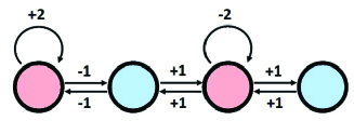
Figure 1: Building the Dynkin diagram of Lie superalgebra $gl\left(m|n\right).$ Here we give the example the Dynkin diagram of $gl\left(3|2\right)$ with weight basis ordered as $\left(\varepsilon_{1},\varepsilon_{2},\delta_{1},\delta_{2},\varepsilon_{3}\right).$

Notice that the ordering of $\left(\varepsilon_{1},\varepsilon_{2},\delta_{1},\delta_{2},\varepsilon_{3}\right)$ is defined modulo the action of the Weyl group $W_{sl_{3}}\times W_{sl_{2}}$ which permutes the basis vectors without changing the $\mathbb{Z}_{2}$-grading.
We end this description by noticing that this graphic representation applies also to the highest weight $\lambda=\lambda_{\text{{a}}}\epsilon_{\text{{a}}}$ of modules of the Lie superalgebra $sl\left(m|n\right).$ Details regarding these graphs are given in the Appendix B.

5 More on Chern-Simons with super- invariance

In this section, we study the L-operators for $SL\left(m|n\right)$ supergroups by using CS theory in the presence of interacting ’t Hooft and Wilson super-lines. First, we revisit useful results regarding the building of $\mathcal{L}_{sl_{m}}.$ We take this occasion to introduce a graphic description to imagine all varieties of the $\mathcal{L}_{sl_{m}}$s; see the Figure 2. Then, we investigate the generalisation of these results to supergroups $SL\left(m|n\right).$ We also give illustrating examples.

5.1 From $SL\left(m\right)$ symmetry to super $SL\left(m|n\right)$

Here, we consider CS theory living on $\mathbb{R}^{2}\times\mathbb{CP}^{1}$ with $SL\left(m\right)$ symmetry and gauge field action (2.3) in the presence of crossing ’t Hooft and Wilson lines. The ’t Hooft line tH${}_{\gamma_{0}}^{\mu}$ sits on the x-axis of the topological plane $\mathbb{R}^{2}$ and the Wilson line W${}_{\xi_{z}}^{\boldsymbol{R}}$ expands along the vertical y-axis as depicted by the Figure 6.

5.1.1 L-operator for $SL\left(m\right)$ symmetry

In the CS theory with $SL\left(m\right)$ gauge symmetry, the oscillator realisation of the L-operator is given by eq(2.1) namely $e^{X}z^{\mathbf{\mu}}e^{Y}$. We revisit below the explicit derivation of its expression by using a projector operator language [39].

$\bullet$ Building L$\left(z\right)$
The explicit construction of the L-operator requires the knowledge of three quantities:
$\left(\mathbf{1}\right)$ the adjoint form of the coweight $\mathbf{\mu}$ which is the magnetic charge operator of tH${}_{\gamma_{0}}^{\mathbf{\mu}}$.
$\left(\mathbf{2}\right)$ the nilpotent matrix operators $X$ and $Y$ obeying the property $X^{k}=Y^{k}=0$ for some positive integer $k$. For $sl\left(m\right)$, this degree $k$ of nilpotency is $k=2$. As we will see later on, this feature holds also for $sl(m|n)$.
To describe the quantities $\left(\mathbf{\mu},X,Y\right)$, we begin by recalling $\left(\mathbf{a}\right)$ the Levi-decomposition of $sl(m)$ with respect to $\mu_{k}$ with label as $1\leq k\leq m-1.$ $\left(\mathbf{b}\right)$ the decomposition of its fundamental representation $\boldsymbol{m}.$ These two decompositions are given by

$$\mathbf{\mu}_{k}:\begin{tabular}[]{lll}$sl(m)$&$\rightarrow$&$\boldsymbol{l}_{\mu_{k}}\oplus\boldsymbol{n}_{+}\oplus\boldsymbol{n}_{-}$\\ $\mathbf{\ }\boldsymbol{m}$&$=$&$\boldsymbol{k}_{1-\frac{k}{m}}\oplus\left(\boldsymbol{m-k}\right)_{-\frac{k}{m}}$\end{tabular}$$ (5.1)

In the first decomposition, the generators of Levi-subalgebra $\boldsymbol{l}_{\mu_{k}}$ and those of the nilpotent sub-algebras $\boldsymbol{n}_{\pm}$ are discriminated by the charges under $\mathbf{\mu}_{k}$; we have $\left[\mathbf{\mu}_{k},\boldsymbol{l}_{\mu_{k}}\right]=0$ and $\left[\mathbf{\mu}_{k},\boldsymbol{n}_{\pm}\right]=\pm\boldsymbol{n}_{\pm}$. In eq(5.1), the $\boldsymbol{l}_{\mu_{k}}$ and $\boldsymbol{n}_{\pm}$ are is given by

$$\boldsymbol{l}_{\mu_{k}}$$

(5.2)

with

$$\dim\boldsymbol{l}_{\mu_{k}}$$

(5.3)

Regarding the decomposition of the fundamental representation $\boldsymbol{m},$ it is given by the direct sum of representations of $sl(k)\oplus sl(m-k)$ namely

$$\boldsymbol{k}_{1-\frac{k}{m}}\text{\qquad},\text{ \qquad}\left(\boldsymbol{m-k}\right)_{-\frac{k}{m}}$$ (5.4)

The lower label refers to the charges of $sl(1)$ generated by $\mathbf{\mu}_{k}.$ The values are constrained by the traceless property of $sl(m)$. From the decomposition $\boldsymbol{m}=\boldsymbol{k}_{1-\frac{k}{m}}\oplus\left(\boldsymbol{m-k}\right)_{-\frac{k}{m}},$ we learn two interesting features [10]:
$\left(\mathbf{i}\right)$ the $\mathbf{\mu}$ operator can be expressed in terms of the orthogonal projectors $\Pi_{\boldsymbol{k}}$ and $\Pi_{\boldsymbol{m-k}}$ on the representations $\boldsymbol{k}_{1-\frac{k}{m}}$ and $\left(\boldsymbol{m-k}\right)_{-\frac{k}{m}}$ as follows

$$\mathbf{\mu}$$

(5.5)

where $\boldsymbol{R}_{i}$ stand for the representations $\boldsymbol{k}_{1-\frac{k}{m}}$ of $sl(k)$ and $\left(\boldsymbol{m-k}\right)_{-\frac{k}{m}}$ of $sl(m-k);$ and where $\Pi_{\boldsymbol{R}_{1}}$ and $\Pi_{\boldsymbol{R}_{2}}$ are projectors satisfying $\Pi_{\boldsymbol{R}_{i}}.\Pi_{\boldsymbol{R}_{j}}=\delta_{ij}\Pi_{\boldsymbol{R}_{i}}$. The coefficients $q_{i}$ are given by

$$q_{i}=Tr\left(\mathbf{\mu}\Pi_{\boldsymbol{R}_{i}}\right).$$ (5.6)

$\left(\mathbf{ii}\right)$ the operators $z^{\mathbf{\mu}}$, $X$ and $Y$ involved in the calculation of $e^{X}z^{\mathbf{\mu}}e^{Y}$ can be also expressed in terms of $\Pi_{\boldsymbol{k}}$ and $\Pi_{\boldsymbol{m-k}}$. For example, we have

$$z^{\mathbf{\mu}}=z^{\frac{m-k}{m}}\Pi_{\boldsymbol{k}}+z^{-\frac{k}{m}}\Pi_{\boldsymbol{m-k}}$$ (5.7)

By using $I_{id}=\Pi_{\boldsymbol{k}}+\Pi_{\boldsymbol{m-k}}$ and $\Pi_{\boldsymbol{R}_{i}}.\Pi_{\boldsymbol{R}_{j}}=\delta_{ij}\Pi_{\boldsymbol{R}_{i}},$ we can split the matrix operators $X$ and $Y$ into four blocks like

$$X_{ij}=\Pi_{\boldsymbol{R}_{i}}X\Pi_{\boldsymbol{R}_{j}}\qquad,\qquad Y_{ij}=\Pi_{\boldsymbol{R}_{i}}Y\Pi_{\boldsymbol{R}_{j}}$$ (5.8)

Substituting into $L=e^{X}z^{\mathbf{\mu}}e^{Y}$, we obtain the generic expression of the L-matrix namely

$$L_{ij}=\Pi_{\boldsymbol{R}_{i}}e^{X}\left(z^{\frac{m-k}{m}}\Pi_{\boldsymbol{k}}+z^{-\frac{k}{m}}\Pi_{\boldsymbol{m-k}}\right)e^{Y}\Pi_{\boldsymbol{R}_{j}}$$ (5.9)

with $\boldsymbol{R}_{1}=\boldsymbol{k}_{1-\frac{k}{m}}$ and $\boldsymbol{R}_{2}=\left(\boldsymbol{m-k}\right)_{-\frac{k}{m}}.$ Moreover, using the property $X^{2}=Y^{2}=0,$ we obtain after some straightforward calculations, the following

$$L=\left(\begin{array}[]{cc}\Pi_{1}\left(z^{\frac{m-k}{m}}+z^{-\frac{k}{m}}XY\right)\Pi_{1}&z^{-\frac{k}{m}}\Pi_{1}X\Pi_{2}\\ z^{-\frac{k}{m}}\Pi_{2}Y\Pi_{1}&z^{-\frac{k}{m}}\Pi_{2}\end{array}\right)$$ (5.10)

with $XY=b^{ai}c_{ai}\Pi_{1}$ where $b^{ai}$ and $c_{ai}$ are Darboux coordinates of the phase space underlying the RLL equation of integrability [13],

$$R_{rs}^{ik}\left(z-w\right)L_{j}^{r}\left(z\right)L_{l}^{s}\left(w\right)=L_{r}^{i}\left(w\right)L_{s}^{k}\left(z\right)R_{jl}^{rs}\left(z-w\right)$$ (5.11)

where $R_{rs}^{ik}\left(z\right)$ is the usual R-matrix of Yang-Baxter equation.

$\bullet$ Levi-decomposition in D- language
Here, we want to show that as far as the $sl\left(m\right)$ is concerned, the Levi-decomposition with respect to $\mu_{k}$ is equivalent to cutting the node labeled by the simple root $\alpha_{k}$ in the Dynkin diagram. We state this correspondence as follows

$$sl(m)$$

                     

(5.12)

where the notation $D_{p-1}$ refers to the Dynkin diagram of $sl\left(p\right)$ and where we have hidden the nilpotent sub-algebras $\boldsymbol{n}_{\pm}$; see also the Figure 2. Notice that $\boldsymbol{n}_{\pm}$ together with $sl(1)$ give the $sl\left(2\right)$ associated with $D_{1}$. The correspondence (5.12) is interesting for two reasons.

$\left(\mathbf{1}\right)$

It indicates that the Levi- splitting (5.1) used in the oscillator realisation of the L-operator can be nicely described by using the language of Dynkin diagram of $sl(m)$ (for short D-language).

$\left(\mathbf{2}\right)$

It offers a guiding algorithm to extend the Levi-decomposition to Lie superalgebras, which to our knowledge, is still an open problem [45, 46]. Because of this lack, we will use this algorithm later on when we study the extension of the Levi-decomposition to $sl(m|n).$ In this regard, it is interesting to notice that in the context of supersymmetric gauge theory, it has been known that the L-operator has an interpretation as a surface operator [59]. It has been also known that the Levi-decomposition is relevant to the surface operator; see, e.g. [60].

Recall that the Dynkin diagram of $sl(m)$ is given by a linear chain with $\left(m-1\right)$ nodes labeled by the $\left(m-1\right)$ simple roots $\alpha_{i}$; see the first graph of the Figure 2 describing $sl_{7}.$ The nodes’ links are given by the intersection matrix

$$K_{ij}=\alpha_{i}.\alpha_{j}$$ (5.13)

which is just the Cartan matrix of $sl(m)$. In this graphic description, the three terms $sl(m-k)\oplus sl(1)\oplus sl(k)$ making $\boldsymbol{l}_{\mu_{k}}$ are nicely described in terms of pieces of the Dynkin diagram as exhibited by (5.12). The three pieces $D_{m-k-1}\oplus D_{1}\oplus D_{k-1}$ are generated by cutting the node $\alpha_{k}$ with label as $2\leq k\leq m-2$; see the Figure 2  for illustration.

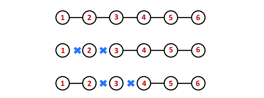
Figure 2: Two Levi-decompositions of $sl_{7}$ in the D-language. The first decomposition is given by cutting the second node corresponding to $\alpha_{2}$. The second decomposition is given by cutting the third node. Generally speaking, there are six ways to cut a node from $sl_{7}$.

The case $k=1$ ( resp. $k=m-1$) concerns the cutting of boundary node $\alpha_{1}$ ( resp. $\alpha_{m-1}$): In this situation, we have the following correspondence

$$sl(m)$$

               

       

(5.14)

5.1.2 Extension to $SL\left(m|n\right)$ symmetry

To extend the construction of the L-operator of $sl\left(m\right)$ to the Lie superalgebra $sl(m|n),$ we use the relationship between $sl\left(m\right)$ and $sl(m|n)$ algebras

$$sl\left(m\right)\subset sl(m|n)_{\bar{0}}\subset sl(m|n)$$ (5.15)

This embedding property holds also for the representations

$$\mathbf{rep}_{sl_{m}}\subset\mathbf{rep}_{sl(m|n)_{\bar{0}}}\subset\mathbf{rep}_{sl(m|n)}$$ (5.16)

$A)$ Field super-action
Here, the $sl(m)$ symmetry of the CS field action (2.3) is promoted to the super $SL(m|n)$ and the usual trace (tr) is promoted to the super-trace (str) [48, 49]; that is:

$$sl(m)$$     ; trace super-trace

(5.17)

So, the generalised CS field action on $\mathbb{R}^{2}\times\mathbb{CP}^{1}$ invariant under $SL(m|n)$ is given by the supertrace of a Lagrangian like $\int dz\wedge\left[str\mathcal{L}_{CS}\right].$ This generalised action reads as follows

$$S_{4dCS}^{sl(m|n)}=\int_{\mathbb{R}^{2}\times\mathbb{CP}^{1}}dz\wedge str\left[\mathcal{A}\wedge d\mathcal{A}+\frac{2}{3}\mathcal{A}\wedge\mathcal{A}\wedge\mathcal{A}\right]$$ (5.18)

In this generalisation, the Chern-Simons gauge field $\mathcal{A}$ is valued in the Lie superalgebra $sl(m|n)$. It has the following expansion

$$\mathcal{A}=\sum_{\text{{ab}}}A^{\text{{ab}}}\mathcal{E}_{\text{{ab}}}$$ (5.19)

where $\mathcal{E}_{\text{{ab}}}$ are the graded generators of $sl(m|n)$ obeying the graded commutation relations (4.7). In terms of these super-generators, the super-trace of the Chern-Simons 3-form

$$\tilde{\Omega}_{3}=\mathcal{A}\wedge d\mathcal{A}+\frac{2}{3}\mathcal{A}\wedge\mathcal{A}\wedge\mathcal{A}$$ (5.20)

is given by

$$str\left(\tilde{\Omega}_{3}\right)=g_{\text{{abcd}}}A^{\text{{ab}}}dA^{\text{{cd}}}+\frac{2}{3}f_{\text{{abcdef}}}A^{\text{{ab}}}A^{\text{{cd}}}A^{\text{{ef}}}$$ (5.21)

where we have set

$$g_{\text{{abcd}}}=str\left(\mathcal{E}_{\text{{ab}}}\mathcal{E}_{\text{{cd}}}\right)\qquad,\qquad f_{\text{{abcdef}}}=str\left(\mathcal{E}_{\text{{ab}}}\mathcal{E}_{\text{{cd}}}\mathcal{E}_{\text{{ef}}}\right)$$ (5.22)

By using the notation (4.9), we can rewrite the development (5.19) like,

$$\mathcal{A}=A^{\text{ab}}\mathcal{E}_{\text{ab}}+A^{\prime\text{ij}}\mathcal{E}_{\text{ij}}^{\prime}+\tilde{A}^{\text{ai}}\mathcal{\tilde{E}}_{\text{ai}}+\tilde{A}^{\prime\text{ia}}\mathcal{\tilde{E}}_{\text{ia}}^{\prime}$$ (5.23)

where the 1-form potentials $A^{\text{ab}}$ and $A^{\prime\text{ij}}$ have an even degree while the $\tilde{A}^{\text{ai}}$ and $\tilde{A}^{\prime\text{ia}}$ have an odd degree. The diagonal $A^{\text{ab}}$ and $A^{\prime\text{ij}}$ are respectively in the adjoints of $sl(m)$ and $sl(n).$ The off-diagonal blocks $\tilde{A}^{\text{ai}}$ and $\tilde{A}^{\prime\text{ia}}$ are fermionic fields contained in the bi-fundamental $sl(m)\oplus sl(n)$. In the super-matrix representation, they are as follows

$$\mathcal{A}=\left(\begin{array}[]{cc}A^{\text{ab}}\mathcal{E}_{\text{ab}}&\tilde{A}^{\text{ai}}\mathcal{\tilde{E}}_{\text{ai}}\\ \tilde{A}^{\prime\text{ia}}\mathcal{\tilde{E}}_{\text{ia}}^{\prime}&A^{\prime\text{ij}}\mathcal{\tilde{E}}_{\text{ij}}\end{array}\right)$$ (5.24)

The 1-form gauge field $A^{\text{{ab}}}=str\left(\mathcal{E}^{\text{{ab}}}\mathcal{A}\right)$ splits explicitly like

$$A^{\text{ab}}$$ ,

,

(5.25)

In the distinguished basis of $gl(m|n)$ with even part $gl(m)\oplus gl(n)$, the $A^{\text{ab}}$ is the gauge field of $gl(m)$ valued in the adjoint $\left(\boldsymbol{m,\bar{m}}\right)$ and the $A^{\prime\text{ij}}$ is the gauge field of $gl(n)$ valued in $\left(\boldsymbol{n,\bar{n}}\right)$. The fields $\tilde{A}^{\text{ai}}$ and $\tilde{A}^{\prime\text{ia}}$ describe topological gauge matter [50, 51] valued in the bi-fundamentals $\left(\boldsymbol{m,\bar{n}}\right)$ and $\left(\boldsymbol{\bar{m},n}\right)$.

$B)$ super-line operators
To extend the bosonic-like Wilson line W${}_{\xi_{z}}^{\boldsymbol{m}}$ of the CS gauge theory to the super- group $SL(m|n)$, we use the representation language to think about this super-line as follows

gauge symmetry fund representation      Wilson line

$$\ \ SL(m)$$

         W

(5.26)

where the fundamental $\boldsymbol{m}$ of $sl\left(m\right)$ is promoted to the fundamental $\boldsymbol{m|n}$ of $sl(m|n)$. In this picture, W${}_{\xi_{z}}^{\boldsymbol{m|n}}$ can be imagined as follows

$$W_{\xi_{z}}^{\boldsymbol{m|n}}=str_{\boldsymbol{m|n}}\left[P\exp\left(\mathop{\displaystyle\oint}\nolimits_{\xi_{z}}\mathcal{A}\right)\right]$$ (5.27)

with $\mathcal{A}=A^{\text{{ab}}}\mathcal{E}_{\text{{ab}}}$ and

$$str\left(\begin{array}[]{cc}A&B\\ C&D\end{array}\right)=trA-trD$$ (5.28)

A diagrammatic representation of the Wilson superline W${}_{\mathrm{\xi}_{z}}^{\boldsymbol{m|n}}$ charged under $SL(m|n)$ is given b the Figure 3.

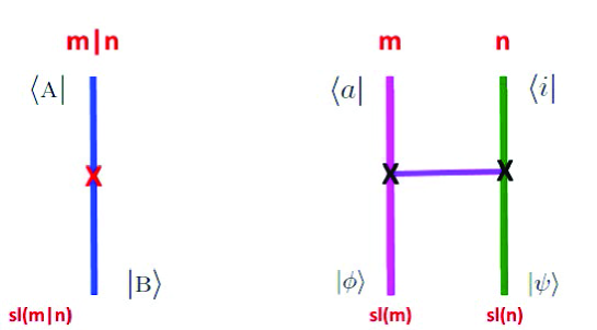
Figure 3: A graphic representation of the Wilson superline $W_{\xi_{z}}^{\boldsymbol{m|n}}$ charged under $sl(m|n)$. On the left, the superline is represented in the topological plane. On the right, the superline is described in terms of graded Wilson lines related by a bridge connecting the two gradations $\mathbf{\bar{0}}$ and $\mathbf{\bar{1}}$. The states $\left|\text{{a}}\right\rangle$ and $\left|\text{{b}}\right\rangle$ can be bosonic and fermionic. The states $\left|a\right\rangle$ are bosonic-like and $\left|i\right\rangle$ are fermionic-like. The states $\left|\phi\right\rangle$ and $\left|\psi\right\rangle$ can be either bosonic or fermionic.

Regarding the magnetically charged ’t Hooft super-line, we think of it below as tH${}_{\mathrm{\gamma}_{\mathrm{0}}}^{\mathbf{\mu}}$having the same extrinsic shape as in the bosonic CS theory, but with the intrinsic bosonic $SL\left(m\right)$ promoted to $SL\left(m|n\right)$. This definition follows from eq(8.4) of appendix A by extending the $g_{I}\left(z\right)$ and $g_{II}\left(z\right)$ to supergroup elements $\tilde{g}_{I}\left(z\right)$ and $\tilde{g}_{II}\left(z\right)$ in $SL(m|n)$. In other words, eq(8.4) generalises as

$$L_{sl_{\boldsymbol{m|n}}}=\tilde{g}_{I}.z^{\mathbf{\tilde{\mu}}}.\tilde{g}_{II}$$ (5.29)

with $\tilde{g}_{I}\left(z\right)$ and $\tilde{g}_{II}\left(z\right)$ belonging to $SL(m|n)$; and $\mathbb{\mu}$ generating the charge group $SL\left(1\right)$ in the even part $SL(m|n)_{0}.$ Notice that using $sl(m|n)_{0}=s\left[gl(m)\oplus gl(n)\right]$, the adjoint form of $\mathbf{\tilde{\mu}}$ has in general two contributions like

$$\mathbf{\tilde{\mu}}=\mathbb{\mu}_{sl_{m}}+\mathbb{\mu}_{sl_{n}}\qquad,\qquad\mathbb{\mu}_{sl_{m}}=\mathbf{\tilde{\mu}.}\Pi_{sl_{m}}\qquad,\qquad\mathbb{\mu}_{sl_{n}}=\mathbf{\tilde{\mu}.}\Pi_{sl_{n}}$$ (5.30)

where $str(\mathbf{\tilde{\mu}})=0$ and $\Pi_{sl_{m}}\$and $\Pi_{sl_{n}}$ are orthogonal projectors on $sl(m)$ and $sl(n)$ respectively; i.e: $\Pi_{sl_{m}}.\Pi_{sl_{n}}=0$. For an illustration; see for instance eq(6.30) given below. Notice that the super-traceless condition reads in terms of the usual trace like $tr(\mathbb{\mu}_{sl_{m}})-tr(\mathbb{\mu}_{sl_{n}})=0.$ By projecting $sl(m|n)_{0}$ down to $sl(m)$ disregarding the $sl(n)$ part, the super-trace condition $str(\mathbf{\tilde{\mu}})=0$ reduces to the familiar $tr(\mathbb{\mu}_{sl_{m}})=0.$
Except for the intrinsic properties we have described above, the extrinsic features of the super-lines are quite similar to $sl\left(m\right).$ In particular, the positions of the two crossing super-lines in the topological plane $\mathbb{R}^{2}$ and the holomorphic $\mathcal{C}$ are as in the bosonic CS theory with $SL\left(m\right)$ gauge symmetry; see the Figure 6. In this regard, we expect that the extension of the YBE and RLL equations (5.11) to supergroups may be also derived from the crossing of the super-lines. From the side of the superspin chains, these algebraic equations were studied in literature; see for instance to [52, 53, 54, 55, 56, 57, 58] and references therein. From the gauge theory side, the super-YBE and the super-RLL equations have not been yet explored. In our formalism, the super-RLL equations are given by the diagram of the Figure 4.

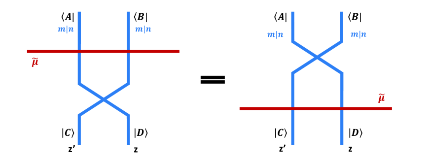
Figure 4: A graphic representation of the RLL equation involving three super-lines. Two ”blue” interacting Wilson super-lines crossed by a ”red ” ’t Hooft super-line. This super-equation contains the usual RLL equation of bosonic like symmetries such as sl(m).

5.2 Decomposing super-Ds with one fermionic node

Here, we give partial results regarding the extension of the decomposition (5.12) concerning $sl(m)$ to the case of the Lie superalgebra $sl(m|n).$ We study three kinds of decompositions of DSDs of $sl(m|n).$ These decompositions are labeled by an integer p constrained as $1\leq p\leq m$ and can be imagined in terms of the breaking pattern

$$sl(m|n)\rightarrow sl(p|0)\oplus sl(m-p|n)$$ (5.31)

The three kinds of decomposition patterns concern the following intervals of the label p:

$\bullet$ the particular case $p=1$.

$\bullet$ the generic case $2\leq p\leq m-1.$

$\bullet$ the special case $p=m$.
This discrimination for the values of p is for convenience; they can be described in a compact way. Notice that the above decomposition can be also applied for the pattern

$$sl(m|n)\rightarrow sl(0|q)\oplus sl(m|n-q)$$ (5.32)

with $1\leq q\leq n$. We omit the details of this case; the results can be read from (5.31).

5.2.1 Cutting the left node in the super $\hat{D}_{m+n-1}$

The decomposition of the DSDs denoted below like $\hat{D}_{m+n-1}$ generalises the correspondence (5.14). It is illustrated on the Figure 5 describing two examples of typical decompositions of $\hat{D}_{6}$: $\left(i\right)$ a bosonic decomposition corresponding to cutting the second node labeled by the bosonic root $\alpha_{2}.$ $\left(ii\right)$ a fermionic decomposition corresponding to cutting the fourth node labeled by the fermionic root $\alpha_{4}.$

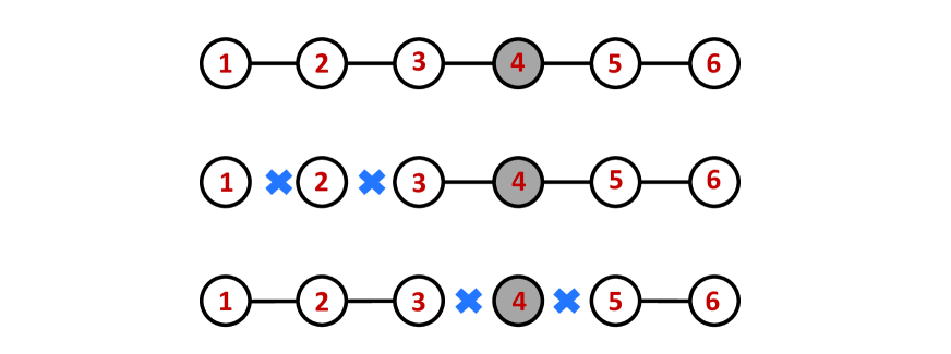
Figure 5: Two decompositions of a DSD of the distinguished Lie superalgebra A_5|1. The first decomposition is given by cutting the second node corresponding to the simple root $\alpha_{2}$. The other decomposition is given by cutting the fermionic (fourth) node.

By cutting the left node of the DSD, that is the node labeled by $\alpha_{1}$ with positive length $\alpha_{1}^{2}=2,$ the super- Dynkin diagram $\hat{D}_{m+n-1}$ breaks into two pieces $D_{1}$ and $\hat{D}_{m+n-2}$ as given by the following correspondence

$$sl(m|n)$$

               

       

(5.33)

Notice that by setting $n=0,$ we recover the bosonic $sl(m)$ case (5.14). Here, the $\hat{D}_{m+n-1}$ refers to the distinguished DSDs of $sl(m|n)$ having $m+n-1$ nodes; one of them is a fermionic; it is labeled by the odd simple root $\tilde{\alpha}_{m}.$ All the other $m+n-2$ nodes are bosonic simple roots as shown in the following table,

simple root $$\ \ \alpha_{1}$$

       degree even   even    odd   even

   length

(5.34)

By cutting the node labeled by $\alpha_{1}$, the root system $\Phi_{sl(m|n)}$ splits into two subsets. The first concerns the root sub-system of $sl(m-1|n)$ containing $\left(m+n-2\right)\left(m+n-1\right)$ roots dispatched as follows

root $$\ \ \ \ \alpha_{ab}$$

value

number

degree        even        even                   odd

(5.35)

This root sub-system $\left\{\beta=\sum n_{i}\alpha_{i}\right\}$ is a subset of $\Phi_{sl_{m|n}};$ it has no dependence in $\alpha_{1}$ as it has been removed. This property can be stated like

$$\frac{\partial\beta}{\partial\alpha_{1}}=0\quad,\quad\beta\in\Phi_{sl_{m|n}}$$ (5.36)

The second subset contains $2\left(m-1\right)+2n$ roots $\beta=\sum n_{i}\alpha_{i};$ it is a subset of $\Phi_{sl_{m|n}}$ with $\partial\beta/\partial\alpha_{1}\neq 0$. These roots are distributed as follows

root $$\ \left\{\pm\alpha_{1b}\right\}$$

value

number

degree            even              odd

(5.37)

The decomposition (5.33) can be checked by calculating the dimensions and the ranks of the $sl(m|n)$ pieces resulting from the breaking

$$sl(m|n)=\boldsymbol{l}_{1}\oplus\boldsymbol{N}_{1}^{+}\oplus\boldsymbol{N}_{1}^{-}$$ (5.38)

where

$$\ \ \ \boldsymbol{l}_{1}$$

(5.39)

and where the nilpotent $\boldsymbol{N}_{1}^{\pm}$ are in the bifundamentals of $gl(1|0)\oplus gl(m-1|n)$. From this splitting, we learn $\dim\left(\boldsymbol{l}_{1}\right)_{\bar{0}}=\left(m+n-1\right)^{2}$ and $\dim\left(\boldsymbol{l}_{1}\right)_{\bar{1}}=2\left(m-1\right)+2n.$ Recall that the Lie superalgebra $gl(m-1|n)$ has dimension $\left(m+n-1\right)^{2}$ and the super-traceless $sl(m-1|n)$ has dimension $\left(m+n-1\right)^{2}-1$; it decomposes like

$$gl(m-1|n)$$

(5.40)

such that the even part of $\boldsymbol{l}_{1}$ is given by the super-traceless

$$\left(\boldsymbol{l}_{1}\right)_{\bar{0}}=s\left[gl(1)\oplus gl(m-1)\oplus gl(n)\right]$$ (5.41)

Then, the nilpotent $\boldsymbol{N}_{1}^{\pm}$ are given by the direct sum of representations $(\boldsymbol{r}_{x}^{gl_{{\small m-1}}},\boldsymbol{r}_{y}^{gl_{{\small n}}})$ of the subalgebra $\left(\boldsymbol{l}_{1}\right)_{\bar{0}}$ with $x,$ $y$ referring to the charge of $gl(1)$. From eq(5.37), we learn

$$\boldsymbol{N}_{1}^{+}$$

(5.42)

The $\left(m-1\right)+n$ generators $X_{\text{{a}}}=\left(X_{a},\mathcal{X}_{i}\right)$ of the nilpotent algebra $\boldsymbol{N}_{1}^{+}$ and the $\left(m-1\right)+n$ generators $Y_{\text{{a}}}=\left(Y_{a},\mathcal{Y}_{i}\right)$ of $\boldsymbol{N}_{1}^{-}$ are realised using the kets $\left|\text{{a}}\right\rangle$ and bra $\left\langle\text{{a}}\right|$ as follows

                             generators degree

$$X_{a}$$ , even

, even

, odd

, odd

(5.43)

They are nilpotent since we have $X_{a}X_{b}=\mathcal{X}_{i}\mathcal{X}_{j}=X_{a}\mathcal{X}_{i}=0$ and the same for the $Y$’s. These properties are interesting for the calculation of the super- Lax operators.

5.2.2 Cutting an internal node $\alpha_{p}$ with $1<p<m-1$

In this generic case, the Lie superalgebra $sl(m|n)$ decomposes like $\boldsymbol{l}_{p}\oplus\boldsymbol{N}_{p}^{+}\oplus\boldsymbol{N}_{p}^{-}$ with the sub-superalgebra $\boldsymbol{l}_{p}$ as

$$\boldsymbol{l}_{p}=s\left[gl(p)\oplus gl(1)\oplus gl(m-p|n)\right]$$ (5.44)

and the nilpotent $\boldsymbol{N}_{p}^{\pm}$ given by the bi-fundamentals of $gl(p)\oplus gl(m-p|n)$ with $\pm 1$ charges under $gl(1).$ Being a superalgebra, the $\boldsymbol{l}_{p}$ decomposes in turns like

$$\ \ \boldsymbol{l}_{p}$$

(5.45)

The decomposition of $sl(m|n)\subset gl(m|n)$ and the associated super- diagram $\hat{D}_{m+n-1}$ generalise the correspondence (5.12). It given by

$$sl(m|n)$$

                     

(5.46)

where we have hidden the nilpotent $\boldsymbol{N}_{p}^{\pm}$. In this generic $1<p<m,$ the simple roots of $sl(m|n)$ are dispatched as follows,

simple root $$\left\{\alpha_{a}\right\}_{{\small 1<a<p}}$$

         degree even even   even odd   even

(5.47)

By cutting the p-th node of the DSD of $sl(m|n)$ labeled by the simple root $\alpha_{p}$, the super $\hat{D}_{m+n-1}$ breaks into three pieces like $D_{p-1}\oplus D_{1}\oplus\hat{D}_{m+n-p-1}$. Then, the root system $\Phi_{sl_{m|n}}$ splits into three subsets as commented below.

$\bullet$ case $\hat{D}_{m+n-p-1}$
The first subset concerns the roots of $sl(m-p|n)$ containing ${\small(m+n-p)(m+n-p-1)}$ elements dispatched as follows

root $$\ \ \ \ \ \pm\alpha_{ab}$$

value

number

degree        even        even       odd

(5.48)

$\bullet$ case $D_{p-1}$
The second subset concerns the roots of $sl(p);$ it contains $p\left(p-1\right)$ even roots given by

$$\pm\alpha_{ab}=\pm\left\{\varepsilon_{a}-\varepsilon_{b}\right\}_{{\small 1\leq a<b\leq p}}$$ (5.49)

$\bullet$ case of bi-fundamentals
The third subset of roots regards the bi-fundamentals $\boldsymbol{N}_{p}^{\pm}$; it contains $2p\left(m-p\right)$ even roots and $2pn$ odd ones as shown on the following table

root $$\ \ \pm\alpha_{ab}$$

value

number

degree            even              odd

(5.50)

Notice that by adding the numbers of the roots in (5.48) and (5.49) as well as (5.50), we obtain the desired equality

$$(m+n-p)(m+n-p-1)+p\left(p-1\right)+2p\left(m-p\right)+2pn=\left(m+n-1\right)\left(m+n\right)$$ (5.51)

Notice also that the algebraic structure of the nilpotent $\boldsymbol{N}_{p}^{\pm}$ can be described by using the bosonic-like symmetry $\left(\boldsymbol{l}_{p}\right)_{\bar{0}}$ given by (5.45) namely $gl(p)\oplus gl(m-p)\oplus gl(n)$ where we have hidden $gl(1)$ as it is an abelian charge operator. We have

$$\boldsymbol{N}_{p}^{+}$$

(5.52)

The $p\left(m-p\right)+pn$ generators $X_{\text{{a}}}=\left(X_{a\dot{b}},\mathcal{X}_{ai}\right)$ of the nilpotent $\boldsymbol{N}_{p}^{+}$ and the $p\left(m-p\right)+pn$ generators $Y_{\text{{a}}}=\left(Y_{a\dot{b}},\mathcal{Y}_{ai}\right)$ of $\boldsymbol{N}_{1}^{-}$ are realised by using the super- kets $\left|\text{{a}}\right\rangle$ and super- bra $\left\langle\text{{a}}\right|$ as follows

                             generators degree

$$X_{a\dot{b}}$$ , , even

, , even

, , odd

, , odd

(5.53)

They are nilpotent since $X_{a\dot{b}}X_{c\dot{d}}=\mathcal{X}_{ai}\mathcal{X}_{bj}=X_{a\dot{b}}\mathcal{X}_{ai}=0$ and the same for the Y’s.

5.2.3 Cutting the fermionic node $\alpha_{m}$

In this case, the Lie superalgebra $sl(m|n)$ decomposes like $\boldsymbol{l}_{m}\oplus\boldsymbol{N}_{m}^{+}\oplus\boldsymbol{N}_{m}^{-}$ with

$$\left(\boldsymbol{l}_{m}\right)_{\bar{0}}$$

(5.54)

and the odd part $\left(\boldsymbol{l}_{m}\right)_{\bar{1}}$ given by

$$\boldsymbol{N}_{m}^{+}=sl(m|n)_{+1},\qquad\boldsymbol{N}_{m}^{-}=sl(m|n)_{-1}$$ (5.55)

The $\boldsymbol{N}_{m}^{\pm}$ are in the bi-fundamentals of $gl(m)\oplus gl(n)$ with $\pm 1$ charges under $sl(1).$ The $\boldsymbol{N}_{m}^{+}$ is given by $(\boldsymbol{m},\boldsymbol{\bar{n}})$ and the $\boldsymbol{N}_{m}^{-}$ is given by $(\boldsymbol{\bar{m}},\boldsymbol{n})$ with generators

                             generators degree

$$\mathcal{X}_{ai}$$ , , odd

, , odd

(5.56)

   

Here as well, the generators are nilpotent because $\mathcal{X}_{ai}\mathcal{X}_{cj}=0$ and the same goes for the Y’s. The novelty for this case is that we have only fermionic generators.
The decomposition of $sl(m|n)$ and its super- diagram $\hat{D}_{m+n-1}$ is a very special case in the sense that it corresponds to cutting the unique fermionic node of the distinguished super- diagram

$$sl(m|n)$$

                     

(5.57)

where we have hidden the nilpotent $\boldsymbol{N}_{m}^{\pm}$. Strictly speaking, the diagram $\hat{D}_{1}$ has one fermionic node corresponding to the unique simple root of $sl(1|1)$ which is fermionic.

6 L-operators for supergroup $SL\left(m|n\right)$

In this section, we focus on the distinguished DSD and construct the super- Lax operators by using the cutting algorithm studied in the previous section. We give two types of L-operators: The first type has mixed bosonic and fermionic phase space variables; see eqs(6.15) and (6.23). The second type is purely fermionic; it corresponds to the $\mathbb{Z}_{2}$-gradation of $SL\left(m|n\right);$ see eqs(6.37) and (6.44).

6.1 L-operators with bosonic and fermionic variables

Here, we construct the super- Lax operator for Chern-Simons theory with $SL(m|n)$ gauge symmetry with $m\neq n$. This is a family of super-line operators associated with the decompositions of the distinguished $sl(m|n)$ given by eq(5.42), (5.52) and (5.54). The L-operator factorises as

$$\mathcal{L}=e^{\Psi}z^{\mathbf{\mu}}e^{\Phi}$$ (6.1)

with $\mathbf{\mu}$ generating $sl\left(1\right)$ and $\Psi,\Phi$ belonging to the nilpotent $N_{\pm}$ sub-superalgebras. The L-operator describes the coupling between a ’t Hooft super-line tH${}_{\mathrm{\gamma}_{0}}^{{}_{\mathbf{\mu}}}$ with magnetic charge $\mathbf{\mu}$ and a Wilson super-line W${}_{\mathrm{\xi}_{z}}^{\boldsymbol{m|n}}.$

6.1.1 More on the decompositions (5.42) and (5.52)

We start by recalling that the $sl(m|n)$ decomposes as $\boldsymbol{l}_{\mu_{p}}^{0}\oplus\boldsymbol{N}_{p}^{+}\oplus\boldsymbol{N}_{p}^{-}$ with graded sub-superalgebra $\boldsymbol{l}_{\mu_{p}}^{0}$ equal to $(\boldsymbol{l}_{\mu_{p}}^{0})_{\bar{0}}\oplus(\boldsymbol{l}_{\mu_{p}}^{0})_{\bar{1}}$ such that

$$(\boldsymbol{l}_{\mu_{p}}^{0})_{\bar{0}}$$

(6.2)

and $\boldsymbol{N}_{p}^{\pm}$ as given by (5.42) and (5.52). The decomposition of the fundamental $\boldsymbol{m|n}$ representation of $sl(m|n)$ with respect to $\mu_{p}$ is given by

$$\boldsymbol{m}$$

(6.3)

where the lower labels refer to the $sl\left(1\right)$ charges. These charges are fixed by the vanishing condition of the super-trace of the representation $\mathbf{m|n}$ reading like,

$$px_{1}+\left(m-p\right)x_{2}=nx_{2}$$ (6.4)

and solved for $m\neq n$ as $x_{1}=\frac{m-p-n}{m-n}$ and $x_{2}=-\frac{p}{m-n}$. Notice that the special case $m=n$ needs a separate construction as it corresponds to the second family of Lie superalgebras listed in the table (4.1). Notice also that the $sl\left(1\right)$ charges allow to construct the generator $\mathbf{\mu}_{p}$ in terms of projectors on three representations:
$\left(\mathbf{1}\right)$ the projector $\Pi_{1}$ on the fundamental representation $\boldsymbol{p}$ of $sl(p).$
$\left(\mathbf{2}\right)\$the projector $\Pi_{2}$ on the representation $\left(\boldsymbol{m-p}\right)$ of $sl(m-p).$
$\left(\mathbf{3}\right)$ the projector $\Pi_{3}$ on the representation $\boldsymbol{n}$ of $sl(n).$
So, we have

$$\mathbf{\mu}_{p}$$

(6.5)

and

$$[\mathbf{\mu}_{p},\Psi]=\Psi\qquad,\qquad[\mathbf{\mu}_{p},\Phi]=-\Phi$$ (6.6)

Observe in passing that $\mathbf{\mu}_{p}$ can be also expressed like $\left(1-\frac{p}{m-n}\right)\Pi_{1}-\frac{p}{m-n}\left(\Pi_{2}+\Pi_{3}\right);$ this feature will be exploited in the appendix C to rederive the result of [29].

6.1.2 The L-operator associated with (6.2)

To calculate the L-operator associated with the decomposition (6.2), notice that the graded matrix operators $\Psi$ and $\Phi$ in (6.1) satisfy (6.6) and can be split into two contributions: $\left(i\right)$ an even contribution $\left.\Psi\right|_{even}=X$ and $\left.\Phi\right|_{even}=Y$. $\left(ii\right)$ an odd contribution $\left.\Psi\right|_{odd}=\mathcal{X}$ and $\left.\Phi\right|_{odd}=\mathcal{Y}$. So, we have

$$\Psi=X+\mathcal{X}\qquad,\qquad\Phi=Y+\mathcal{Y}$$ (6.7)

The $X$ and $Y$ are generated by the bosonic generators $X_{a\dot{b}}$ and $Y^{a\dot{b}}$; they read as follows

$$X=\sum_{a=1}^{p}\sum_{\dot{b}=p+1}^{m}\mathrm{b}^{a\dot{b}}X_{a\dot{b}}\qquad,\qquad Y=\sum_{a=1}^{p}\sum_{\dot{b}=p+1}^{m}\mathrm{c}_{\dot{b}a}Y^{\dot{b}a}$$ (6.8)

where $\mathrm{b}^{a\dot{b}}$ and $\mathrm{c}_{\dot{b}a}$ are bosonic-like Darboux coordinates. The $\mathcal{X}$ and $\mathcal{Y}$ are generated by fermionic generators $\mathcal{X}_{ai}$ and $\mathcal{Y}^{ia}$; they are given by

$$\mathcal{X}=\sum_{a=1}^{p}\sum_{i=1}^{n}\mathrm{\beta}^{ai}\mathcal{X}_{ai}\qquad,\qquad\mathcal{Y}=\sum_{a=1}^{p}\sum_{i=1}^{n}\mathrm{\gamma}_{ia}\mathcal{Y}^{ia}$$ (6.9)

where $\mathrm{\beta}^{ai}$ and $\mathrm{\gamma}_{ia}$ are fermionic-like phase space variables.
The explicit expression of $X_{a\dot{b}}$ and $Y^{\dot{b}a}$ as well as those of $\mathcal{X}_{ai}$ and $\mathcal{Y}^{ia}$ are given by (5.53). They satisfy the useful features

$$\Pi_{1}X$$ , , ,

, , ,

(6.10)

and

$$\Pi_{1}\mathcal{X}$$ , , ,

, , ,

(6.11)

as well as

$$X\Pi_{3}=\Pi_{3}Y=0,\qquad\mathcal{X}\Pi_{3}=\mathcal{X},\qquad\Pi_{3}\mathcal{Y}=\mathcal{Y}$$ (6.12)

These relations indicate that $\Psi\Pi_{1}=0$ and $\Psi\Pi_{2}=\Psi$ while $\Pi_{2}\Phi=\Phi$ and $\Phi\Pi_{2}=0$. Notice also that these matrices satisfy $X^{2}=Y^{2}=0$ and $\mathcal{X}^{2}=\mathcal{Y}^{2}=0$ as well as $X\mathcal{X}=X\mathcal{Y}=0$ and $Y\mathcal{X}=Y\mathcal{Y}=0$. By using $\Psi=X+\mathcal{X}$ and $\Phi=Y+\mathcal{Y}$, we also have $\Psi^{2}=0$ and $\Phi^{2}=0$. So, the super - Lax operator $\mathcal{L}=e^{\Psi}z^{\mathbf{\mu}}e^{\Phi}$ reads as follows

$$\mathcal{L}=z^{\mathbf{\mu}_{p}}+z^{\mathbf{\mu}_{p}}\Phi+\Psi z^{\mathbf{\mu}_{p}}+\Psi z^{\mathbf{\mu}_{p}}\Phi$$ (6.13)

Substituting (6.5), we can put the above relation into the form

$$\mathcal{L}$$

(6.14)

Then, using the properties (6.10-6.12), we end up with

$$\mathcal{L}=\left(\begin{array}[]{ccc}z^{\frac{m-p-n}{m-n}}\Pi_{1}+z^{-\frac{p}{m-n}}\Pi_{1}\Psi\Phi\Pi_{1}&z^{-\frac{p}{m-n}}\Pi_{1}\Psi\Pi_{2}&z^{-\frac{p}{m-n}}\Pi_{1}\Psi\Pi_{3}\\ z^{-\frac{p}{m-n}}\Pi_{2}\Phi\Pi_{1}&z^{-\frac{p}{m-n}}\Pi_{2}&0\\ z^{-\frac{p}{m-n}}\Pi_{3}\Phi\Pi_{1}&0&z^{-\frac{p}{m-n}}\Pi_{3}\end{array}\right)\text{ }$$ (6.15)

having the remarkable $\Pi_{1}\Psi\Phi\Pi_{1}$ mixing bosons and fermions like $\mathrm{b}^{b\dot{b}}\mathrm{c}_{\dot{b}a}+\mathrm{\beta}^{bi}\mathrm{\gamma}_{ia}$. The quadratic term $\mathrm{b}^{b\dot{b}}\mathrm{c}_{\dot{b}a}$ can be put in correspondence with the energy operator of $p\left(m-p\right)$ free bosonic harmonic oscillators. However, the term $\mathrm{\beta}^{bk}\mathrm{\gamma}_{ka}$ describes the energy operator of $pn$ free fermionic harmonic oscillators. Below, we shed more light on this aspect by investigating the quantum version of eq(6.15).

6.1.3 Quantum Lax operator $\mathcal{\hat{L}}$

To get more insight into the classical Lax super-operator (6.15) and in order to compare with known results obtained in the literature of integrable superspin chain using the Yangian algebra $\mathcal{Y}\left(sl\left(m|n\right)\right)$, we investigate here the quantum $\mathcal{\hat{L}}$ associated with the classical $\mathcal{L}$ (6.15). To that purpose, we proceed in four steps as described below: 
$\left(\mathbf{1}\right)$ We start from eq(6.15) and substitute $X$ and $Y$ as well as $\mathcal{X}$ and $\mathcal{Y}$ by their expressions in terms of the classical oscillators. Putting eqs(6.8) and (6.9) into (6.15), we obtain a $3\times 3$ block graded matrix of the form

$$\mathcal{L}_{A}^{B}=\left(\begin{array}[]{ccc}\mathcal{L}_{a}^{b}&\mathcal{L}_{a}^{\dot{b}}&\mathcal{L}_{a}^{j}\\ \mathcal{L}_{\dot{a}}^{b}&\mathcal{L}_{\dot{a}}^{\dot{b}}&\mathcal{L}_{\dot{a}}^{j}\\ \mathcal{L}_{i}^{a}&\mathcal{L}_{i}^{\dot{b}}&\mathcal{L}_{i}^{j}\end{array}\right)$$ (6.16)

with entries as follows

$$\mathcal{L}_{A}^{B}=\left(\begin{array}[]{ccc}z^{\frac{m-p-n}{m-n}}\delta_{a}^{b}+z^{-\frac{p}{m-n}}\mathrm{b}^{b\dot{b}}\mathrm{c}_{\dot{b}a}\mathbf{+}z^{-\frac{p}{m-n}}\mathrm{\beta}^{bk}\mathrm{\gamma}_{ka}&z^{-\frac{p}{m-n}}\delta_{ac}\mathrm{b}^{c\dot{b}}&z^{-\frac{p}{m-n}}\delta_{ac}\mathrm{\beta}^{cj}\\ z^{-\frac{p}{m-n}}\mathrm{c}_{\dot{a}c}\delta^{cb}&z^{-\frac{p}{m-n}}\delta_{\dot{a}}^{\dot{b}}&0\\ z^{-\frac{p}{m-n}}\mathrm{\gamma}_{ic}\delta^{cb}&0&z^{-\frac{p}{m-n}}\delta_{i}^{j}\end{array}\right)$$ (6.17)

$\left(\mathbf{2}\right)$ In the above expression of the Lax operator (6.17), the products $\mathrm{b}^{b\dot{b}}\mathrm{c}_{\dot{b}a}$ and $\mathrm{\beta}^{bk}\mathrm{\gamma}_{ka}$ are classical; they can be respectively thought of as

$$\mathrm{b}^{b\dot{b}}\mathrm{c}_{\dot{b}a}$$

(6.18)

with $\left(i\right)$ bosonic $\mathrm{b}^{b\dot{b}}$ and $\mathrm{c}_{\dot{b}a}$ tensors represented by the following $p\times\left(m-p\right)$ and $\left(m-p\right)\times p$ rectangular matrices

$$\mathrm{b}^{b\dot{b}}=\left(\begin{array}[]{ccc}\mathrm{b}^{1\dot{1}}&\cdots&\mathrm{b}^{1\dot{p}}\\ \vdots&\ddots&\vdots\\ \mathrm{b}^{p\dot{1}}&\cdots&\mathrm{b}^{p\dot{p}}\end{array}\right),\qquad\mathrm{c}_{\dot{b}a}=\left(\begin{array}[]{ccc}\mathrm{c}_{\dot{1}1}&\cdots&\mathrm{c}_{\dot{1}p}\\ \vdots&\ddots&\vdots\\ \mathrm{c}_{\dot{p}1}&\cdots&\mathrm{c}_{\dot{p}p}\end{array}\right)$$ (6.19)

with $\dot{p}=m-p$; and $\left(ii\right)$ fermionic $\mathrm{\beta}^{bk}$ and $\mathrm{\gamma}_{ka}$ tensors represented by the $p\times n$ and $n\times p$ rectangular matrices

$$\mathrm{\beta}^{bk}=\left(\begin{array}[]{ccc}\mathrm{\beta}^{11}&\cdots&\mathrm{\beta}^{1n}\\ \vdots&\ddots&\vdots\\ \mathrm{\beta}^{p1}&\cdots&\mathrm{\beta}^{pn}\end{array}\right),\qquad\mathrm{\gamma}_{ka}=\left(\begin{array}[]{ccc}\mathrm{\gamma}_{11}&\cdots&\mathrm{\gamma}_{1p}\\ \vdots&\ddots&\vdots\\ \mathrm{\gamma}_{n1}&\cdots&\mathrm{\gamma}_{np}\end{array}\right)$$ (6.20)

$\left(\mathbf{3}\right)$ At the quantum level, the bosonic $\mathrm{b}^{a\dot{b}}$ and $\mathrm{c}_{\dot{a}b}$ as well as the fermionic $\mathrm{\beta}^{ai}$ and $\mathrm{\gamma}_{ia}$ are promoted to the creation $\mathrm{\hat{b}}^{a\dot{b}}$ and annihilation $\mathrm{\hat{c}}_{\dot{a}b}$ operators as well as the creation $\mathrm{\hat{\beta}}^{ai}$ and the annihilation $\mathrm{\hat{\gamma}}_{ia}$. In this regard, notice that in the $su(m|n)$ unitary theory, these creation and annihilation operators are related like $\mathrm{\hat{b}}^{a\dot{b}}=(\mathrm{\hat{c}}_{\dot{b}a})^{\dagger}$ and $\mathrm{\hat{\beta}}^{ai}=(\mathrm{\hat{\gamma}}_{ia})^{\dagger}$. In the 4D super Chern-Simons theory, the unitary gauge symmetry is complexified like $sl(m|n).$ Notice also that the usual classical Poisson bracket of the $\mathbb{Z}_{2}$- graded phase space variables are replaced in quantum mechanics by the following graded canonical commutation relations

$$\begin{tabular}[]{lll}$[\mathrm{\hat{c}}_{\dot{c}d},\mathrm{\hat{b}}^{a\dot{b}}]$&$=$&$\delta_{\dot{c}}^{\dot{b}}\delta_{d}^{a}$\\ $[\mathrm{\hat{b}}^{a\dot{b}},\mathrm{\hat{b}}^{d\dot{c}}]$&$=$&$0$\\ $\left[\mathrm{\hat{c}}_{\dot{b}a},\mathrm{\hat{c}}_{\dot{c}d}\right]$&$=$&$0$\end{tabular}\qquad,\qquad\begin{tabular}[]{lll}$\{\mathrm{\hat{\gamma}}_{jb},\mathrm{\hat{\beta}}^{ai}\}$&$=$&$\delta_{b}^{a}\delta_{j}^{i}$\\ $\{\mathrm{\hat{\beta}}^{ai},\mathrm{\hat{\beta}}^{bj}\}$&$=$&$0$\\ $\{\mathrm{\hat{\gamma}}_{ia},\mathrm{\hat{\gamma}}_{jb}\}$&$=$&$0$\end{tabular}$$ (6.21)

and $[\mathrm{\hat{c}}_{\dot{c}d},\mathrm{\hat{\beta}}^{ai}]=[\mathrm{\hat{c}}_{\dot{c}d},\mathrm{\hat{\gamma}}_{jb}]=0$ as well as $[\mathrm{\hat{b}}^{d\dot{c}},\mathrm{\hat{\beta}}^{ai}]=[\mathrm{\hat{b}}^{d\dot{c}},\mathrm{\hat{\gamma}}_{jb}]=0$.
$\left(\mathbf{4}\right)$ Under the substitution $\left(b,c\right)\rightarrow(\hat{b},\hat{c})$ and $\left(\beta,\gamma\right)\rightarrow(\hat{\beta},\hat{\gamma}),$ the classical eq(6.18) gets promoted to operators as follows

$$\frac{1}{2}\left(\mathrm{\hat{b}}^{b\dot{d}}\mathrm{\hat{c}}_{\dot{d}a}+\mathrm{\hat{c}}_{\dot{d}a}\mathrm{\hat{b}}^{b\dot{d}}\right)$$

(6.22)

Substituting these quantum expressions into (6.17), we obtain the explicit oscillator realisation of the quantum Lax operator namely

$$\mathcal{\hat{L}}_{A}^{B}=\left(\begin{array}[]{ccc}z^{\frac{m-p-n}{m-n}}\delta_{a}^{b}+z^{-\frac{p}{m-n}}\hat{K}_{a}^{b}&z^{-\frac{p}{m-n}}\delta_{ac}\mathrm{\hat{b}}^{c\dot{b}}&z^{-\frac{p}{m-n}}\delta_{ac}\mathrm{\hat{\beta}}^{cj}\\ z^{-\frac{p}{m-n}}\mathrm{\hat{c}}_{\dot{a}c}\delta^{cb}&z^{-\frac{p}{m-n}}\delta_{\dot{a}}^{\dot{b}}&0\\ z^{-\frac{p}{m-n}}\mathrm{\hat{\gamma}}_{ic}\delta^{cb}&0&z^{-\frac{p}{m-n}}\delta_{i}^{j}\end{array}\right)$$ (6.23)

with

$$\hat{K}_{a}^{b}=\mathrm{\hat{b}}^{b\dot{d}}\mathrm{\hat{c}}_{\dot{d}a}+\mathrm{\hat{\beta}}^{bk}\mathrm{\hat{\gamma}}_{ka}+\left[\frac{p\left(m-p\right)}{2}-\frac{pn}{2}\right]\delta_{a}^{b}$$ (6.24)

This result, obtained from the 4D super Chern-Simons theory, can be compared with the quantum Lax operator (2.20) in [29] calculated using the super Yangian $Y\left(su\left(m|n\right)\right)$ representation.  Actually, we can multiply this graded matrix by the quantity $z^{-\frac{p}{m-n}}$ to obtain

$$\mathcal{\hat{L}}_{A}^{B}=\left(\begin{array}[]{ccc}z\delta_{a}^{b}+\hat{K}_{a}^{b}&\delta_{ac}\mathrm{\hat{b}}^{c\dot{b}}&\delta_{ac}\mathrm{\hat{\beta}}^{cj}\\ \mathrm{\hat{c}}_{\dot{a}c}\delta^{cb}&\delta_{\dot{a}}^{\dot{b}}&0\\ \mathrm{\hat{\gamma}}_{ic}\delta^{cb}&0&\delta_{i}^{j}\end{array}\right)$$ (6.25)

Note that the multiplication by a function of the spectral parameter does not affect the RLL equation [13, 32]. More details concerning the comparison between these results and those obtained in [29] are reported in appendix C.
Thanks to these results, we can rely on the consistency of the CS theory approach based on the decomposition of Lie superalgebras to state that the study performed here for one fermionic node can be straightforwardly extended to $\left(i\right)$ the case of several fermionic nodes of $sl(m|n);$ and to $\left(ii\right)$ the other classical Lie superalgebras of table (4.1) such as the orthosymplectic $osp\left(m|2n\right)$ spin chain.

6.2 Pure fermionic L-operator

This is an interesting decomposition of the Lie superalgebra $sl(m|n)$ with distinguished DSD. It corresponds to cutting of the unique fermionic node $\tilde{\alpha}_{m}$ of the distinguished Dynkin super- graph. This decomposition coincides with the usual $\mathbb{Z}_{2}$-gradation of the Lie superalgebra

$$sl(m|n)=sl(m|n)_{\bar{0}}\oplus sl(m|n)_{\bar{1}}$$ (6.26)

Here, we begin by calculating the classical Lax matrix $L$ associated with cutting $\tilde{\alpha}_{m}$ in $\hat{D}_{m+n-1}$, then we investigate its quantum version $\hat{L}$.

6.2.1 Constructing the classical Lax matrix

In the pure fermionic case, the Lie superalgebra decomposes as in (5.54). Besides $\left(\boldsymbol{l}_{m}\right)_{\bar{0}}=s\left[gl(m)\oplus gl(n)\right]$ and the nilpotent $\boldsymbol{N}_{+}=sl(m-1|n)_{+1}$ and $\boldsymbol{N}_{-}=sl(m-1|n)_{-1},$ we need the decomposition of the fundamental $\boldsymbol{m|n}$ representation of $sl(m|n).$ We have

$$\boldsymbol{m|n}=\left(\boldsymbol{m}_{x},\boldsymbol{n}_{y}\right)$$ (6.27)

with lower labels $x$ and $y$ referring to the $sl\left(1\right)$ charges. These charges are determined by the vanishing condition of the supertrace namely $mx-ny=0$ which is solved as follows

$$x=\frac{-n}{m-n}\qquad,\qquad y=\frac{-m}{m-n}$$ (6.28)

Notice that this solution corresponds just to setting $p=m$ in (6.4). These charges allow to construct the generator of the charge operator $\mathbf{\mu}$ in terms of two projectors $\Pi_{1}$ and $\Pi_{2}$ on the representations $\boldsymbol{m}$ of $sl(m)$ and $\boldsymbol{n}$ of $sl(n).$ Using the kets $\left|a\right\rangle$ of even degree generating the $\boldsymbol{m}$ and the kets $\left|m+i\right\rangle$ of odd degree generating $\boldsymbol{n},$ we have

$$\Pi_{1}=\sum_{a=1}^{m}\left|a\right\rangle\left\langle a\right|\qquad,\qquad\Pi_{2}=\sum_{i=1}^{n}\left|m+i\right\rangle\left\langle m+i\right|$$ (6.29)

where $\Pi_{1}$ is the projector on $sl\left(m\right)$ sector in the even part $sl\left(m|n\right)_{\bar{0}}$ of the Lie superalgebra and $\Pi_{2}$ is the projector on its $sl\left(n\right)$ sector. The generator of $gl\left(1\right)$ is then given by

$$\mathbf{\mu}=\frac{n}{n-m}\Pi_{1}+\frac{m}{n-m}\Pi_{2}$$ (6.30)

The $\Psi$ and $\Phi$ nilpotent matrices in (6.1) read as

$$\Psi=\sum_{a=1}^{m}\sum_{i=1}^{n}\mathrm{\beta}^{ai}\mathcal{X}_{ai}\qquad,\qquad\Phi=\sum_{a=1}^{m}\sum_{i=1}^{n}\mathrm{\gamma}_{ia}\mathcal{Y}^{ia}$$ (6.31)

where

$$\mathcal{X}_{ai}=\left|a\right\rangle\left\langle m+i\right|\qquad,\qquad\mathcal{Y}^{ia}=\left|m+i\right\rangle\left\langle a\right|$$ (6.32)

with $\mathrm{\beta}^{ai}$ and $\mathrm{\gamma}_{ia}$ describing $mn$ fermionic phase space coordinates. This realisation satisfies some properties, in particular

$$\Pi_{1}\Psi$$

(6.33)

showing that

$$\left[\mathbf{\mu},\Psi\right]=\Psi\qquad,\qquad\left[\mathbf{\mu},\Phi\right]=-\Phi$$ (6.34)

Moreover, using the properties $\Psi^{2}=\Phi^{2}=0,$ we have $e^{\Psi}=1+\Psi$ and $e^{\Phi}=1+\Phi.$ Putting back into the L-operator (6.1), we obtain

$$\mathcal{L}$$

(6.35)

Substituting $\Pi_{1}\Phi=0$ and $\Psi\Pi_{1}=0$ as well as $\Phi\Pi_{2}=0$ and $\Pi_{2}\Psi=0$, the above expression reduces to

$$\mathcal{L}$$

(6.36)

It reads in super matrix language as follows

$$\mathcal{L}=\left(\begin{array}[]{cc}z^{\frac{n}{n-m}}\Pi_{1}+z^{\frac{m}{n-m}}\Pi_{1}\Psi\Phi\Pi_{1}&z^{\frac{m}{n-m}}\Pi_{1}\Psi\Pi_{2}\\ z^{\frac{m}{n-m}}\Pi_{2}\Phi\Pi_{1}&z^{\frac{m}{n-m}}\Pi_{2}\end{array}\right)$$ (6.37)

where $\Pi_{1}\left(\Psi\Phi\right)\Pi_{1}$ is given by $\sum_{k}\mathrm{\beta}^{bk}\mathrm{\gamma}_{ka}.$ Notice that the term $\mathrm{\beta}^{bk}\mathrm{\gamma}_{ka}$ can be put in correspondence with the energy of $mn$ free fermionic harmonic oscillators as described below.

6.2.2 Quantum version of eq(6.37)

To derive the quantum version $\mathcal{\hat{L}}$ associated with the classical (6.37) and its properties, we use the correspondence between the phase space variables and the quantum oscillators. We determine $\mathcal{\hat{L}}$ by repeating the analysis that we have done in the sub-subsection 6.1.2 to the fermionic oscillators. To that purpose, we perform this derivation by following four steps as follows.
$\left(\mathbf{1}\right)$ We substitute the $\Psi$ and $\Phi$ in (6.37) by their expressions in terms of the classical fermionic oscillators $\mathrm{\beta}^{bk}$ and $\mathrm{\gamma}_{ka}$. By putting eq(6.31) into (6.37), we obtain the following $2\times 2$ block matrix

$$\mathcal{L}_{B}^{A}=\left(\begin{array}[]{cc}\mathcal{L}_{b}^{a}&\mathcal{L}_{j}^{a}\\ \mathcal{L}_{i}^{b}&\mathcal{L}_{ij}\end{array}\right)$$ (6.38)

with entries as follows

$$\mathcal{L}_{A}^{B}=\left(\begin{array}[]{cc}z^{\frac{n}{n-m}}\delta_{a}^{b}+z^{\frac{m}{n-m}}\mathrm{\beta}^{bk}\mathrm{\gamma}_{ka}&z^{\frac{m}{n-m}}\delta_{ab}\mathrm{\beta}^{bj}\\ z^{\frac{m}{n-m}}\mathrm{\gamma}_{ic}\delta^{cb}&z^{\frac{m}{n-m}}\delta_{i}^{j}\end{array}\right)$$ (6.39)

$\left(\mathbf{2}\right)$ We replace the product $\mathrm{\beta}^{bk}\mathrm{\gamma}_{ka}$ in the above classical Lax matrix (6.39) by the following equivalent expression where $\mathrm{\beta}^{bk}$ and $\mathrm{\gamma}_{ka}$ are treated on equal footing,

$$\mathrm{\beta}^{bk}\mathrm{\gamma}_{ka}=\frac{1}{2}\left(\mathrm{\beta}^{bk}\mathrm{\gamma}_{ka}-\mathrm{\gamma}_{ka}\mathrm{\beta}^{bk}\right)$$ (6.40)

with $\mathrm{\beta}^{bk}$ and $\mathrm{\gamma}_{ka}$ given by the following $m\times n$ and $n\times m$ rectangular matrices

$$\mathrm{\beta}^{bj}=\left(\begin{array}[]{ccc}\mathrm{\beta}^{11}&\cdots&\mathrm{\beta}^{1n}\\ \vdots&\ddots&\vdots\\ \mathrm{\beta}^{m1}&\cdots&\mathrm{\beta}^{mn}\end{array}\right),\qquad\mathrm{\gamma}_{ia}=\left(\begin{array}[]{ccc}\mathrm{\gamma}_{11}&\cdots&\mathrm{\gamma}_{1m}\\ \vdots&\ddots&\vdots\\ \mathrm{\gamma}_{n1}&\cdots&\mathrm{\gamma}_{nm}\end{array}\right)$$ (6.41)

$\left(\mathbf{3}\right)$ At the quantum level, the classical fermionic oscillators $\mathrm{\beta}^{bj}$ and $\mathrm{\gamma}_{ia}$ are promoted to the creation $\mathrm{\hat{\beta}}^{bj}$ and the annihilation $\mathrm{\hat{\gamma}}_{ia}$ operators satisfying the following graded canonical commutation relations

$$\{\mathrm{\hat{\gamma}}_{ia},\mathrm{\hat{\beta}}^{bj}\}$$

(6.42)

As noticed before regarding the $su(m|n)$ unitary theory, we have the relation $\mathrm{\hat{\beta}}^{ai}=(\mathrm{\hat{\gamma}}_{ia})^{\dagger}.$ By using this quantum extension, the classical $\mathbf{(}\beta\gamma-\gamma\beta\mathbf{)}/2$ gets promoted in turns to the quantum operator $\mathbf{(}\hat{\beta}\hat{\gamma}-\hat{\gamma}\hat{\beta}\mathbf{)}/2.$ Then, using (6.42), we can also express $\mathbf{(}\hat{\beta}\hat{\gamma}-\hat{\gamma}\hat{\beta}\mathbf{)}/2$ as a normal ordered operator with the creation operators $\hat{\beta}$ put on the left like $\mathrm{\beta}^{bk}\mathrm{\gamma}_{ka}-\left(mn/2\right)\delta_{a}^{b}$. So, eq(6.40) gets replaced by the following normal ordered quantum quantity

$$\frac{1}{2}\left(\mathrm{\hat{\beta}}^{bk}\mathrm{\hat{\gamma}}_{ka}-\mathrm{\hat{\gamma}}_{ka}\mathrm{\hat{\beta}}^{bk}\right)=\mathrm{\hat{\beta}}^{bk}\mathrm{\hat{\gamma}}_{ka}-\frac{mn}{2}\delta_{a}^{b}$$ (6.43)

$\left(\mathbf{3}\right)$ Substituting the above quantum relation into eq(6.39), we obtain the quantum Lax operator $\mathcal{\hat{L}}$ given by

$$\mathcal{\hat{L}}_{A}^{B}=\left(\begin{array}[]{cc}z^{\frac{n}{n-m}}\delta_{a}^{b}+z^{\frac{m}{n-m}}\left(\mathrm{\hat{\beta}}^{bk}\mathrm{\hat{\gamma}}_{ka}-\frac{mn}{2}\delta_{a}^{b}\right)&z^{\frac{m}{n-m}}\delta_{ab}\mathrm{\hat{\beta}}^{bj}\\ z^{\frac{m}{n-m}}\mathrm{\hat{\gamma}}_{ic}\delta^{cb}&z^{\frac{m}{n-m}}\delta_{i}^{j}\end{array}\right)$$ (6.44)

By multiplying this relation by $z^{-\frac{m}{n-m}}$, the above graded matrix becomes

$$\mathcal{\hat{L}}_{A}^{B}=\left(\begin{array}[]{cc}z\delta_{a}^{b}+\left(\mathrm{\hat{\beta}}^{bk}\mathrm{\hat{\gamma}}_{ka}-\frac{mn}{2}\delta_{a}^{b}\right)&\delta_{ab}\mathrm{\hat{\beta}}^{bj}\\ \mathrm{\hat{\gamma}}_{ic}\delta^{cb}&\delta_{i}^{j}\end{array}\right)$$ (6.45)

7 Conclusion and comments

In this paper, we investigated the 4D Chern-Simons theory with gauge symmetry given by the $SL(m|n)$ super-group family ($m\neq n$) and constructed the super- Lax operator solving the RLL equations of the superspin chain. We described the Wilson and ’t Hooft super-lines for the $SL(m|n)$ symmetry and explored their interaction and their implementation in the extended 4D CS super- gauge theory. We also developed a DSDs algorithm for the distinguished basis of $sl(m|n)$ to generalise the Levi- decomposition of Lie algebras to the Lie superalgebras. Our findings agree with partial results obtained in literature on integrable superspin chains. The solutions for $SL(m|n)$ are of two types: a generic one having a mixture between bosonic and fermionic oscillators, and a special purely fermionic type corresponding to the $\mathbb{Z}_{2}$-gradation of $sl(m|n)$.
To perform this study, we started by revisiting the explicit derivation of the expression of the L-operator in 4D CS theory with bosonic gauge symmetry by following the method of Costello-Gaiotto-Yagi used in [13]. We also investigated the holomorphy of $L\left(z\right)$ and described properties of interacting Wilson and ’t Hooft lines. We showed how the Dirac singularity of the magnetic ’t Hooft line lead to an exact description of the oscillator Lax operator for the XXX spin chains with bosonic symmetry.
Then, we worked out the differential equation $\mathcal{D}L=0$ solved by the CGY realisation of the L-operator. We also gave a link of this differential equation with the usual time evolution equation of the Lax operator. We used the algebraic structure of $\mathcal{D}L=0$ to motivate the generalisation of the L-operator to supergroups. As illustration, we considered two particular symmetries: $\left(i\right)$ the bosonic $GL\left(2\right)$ as a simple representative of $GL\left(m\right)$. $\left(ii\right)$ the supergroup $GL\left(1|1\right)$ as a representative of $GL(m|n).$
After that, we investigated the general case of 4D CS with supergroups by focussing on the $sl(m|n)$ family. As there is no known extension for the Levi-theorem concerning the decomposition of Lie superalgebras, we developed an algorithm to circumvent this lack. This algorithm, which uses the Dynkin diagram language, has been checked in the case of bosonic Lie algebras to be just a rephrasing of the Levi-theorem. The extension to Lie superalgebras is somehow subtle because a given Lie superalgebra has in general several representative DSDs. In this context, recall that a bosonic finite dimensional Lie algebra has one Dynkin diagram. But this is not true for Lie superalgebras as described in section 4. As a first step towards the construction of the Lax operators for classical gauge supergroups, we focused our attention on the particular family of distinguished $sl(m|n).$ For this family, we showed that the Levi-theorem extends naturally as detailed in section 5. We used this result to derive the various types of super- Lax operators for the distinguished DSDs containing one fermionic node.
We hope to return to complete this investigation by performing three more steps in the study of L-operators of Lie superalgebras. First, enlarge the construction to other classical Lie superalgebras like $A(m|m)$, $B(m|n)$, $C(m+1)$ and $D(m|n)$. Second, extend the present $sl(m|n)$ study to DSDs with two fermionic nodes and more. Third, use the so-called Gauge/Bethe correspondence to work out D-brane realisations of the superspin chains in type II strings.

8 Appendices

Here we provide complementary materials that are useful for this investigation. We give two appendices A and B. In appendix A, we revisit the derivation of the L-operators in 4D CS with bosonic gauge symmetries and their properties. In section B, we describe the Verma modules of $sl(m|n).$

8.1 Appendix A: L-operators in 4D CS theory

First, we study the link between Dirac singularity of monopoles and the Lax operator obtained in [13]. Then, we revisit the explicit derivation of the minuscule Lax operators by using Levi-decomposition of gauge symmetries.

8.1.1 From Dirac singularity to the L-operator

Following [13], a similar analysis to the Yang-Mills theory monopoles holds for the 4D-CS theory in the presence of a ’t Hooft line with magnetic charge given by the coweight $\mu$. In this case, the special behaviour of the singular gauge field implies dividing the region surrounding the ’t Hooft line into the two intersecting regions $U_{I}$ and $U_{2}$ with line intersection $U_{I}\cap U_{II}=\mathrm{\gamma}_{0}$. By choosing the ’t Hooft line $\mathrm{\gamma}_{0}$ as sitting on the x-axis $(y=0)$ of the topological plane $\mathbb{R}^{2}$ and at $z=0$ of the holomorphic line, we have

$$U_{I}$$

(8.1)

On the region $U_{I},$ we have a trivialised gauge field described by a $G$-valued holomorphic function that needs to be regular at $z=0$, say a holomorphic gauge transformation $\mathfrak{g}_{I}(z)\in G_{[[z]]}$. The same behaviour is valid for the region $U_{II}$ where we have $\mathfrak{g}_{II}(z)\in G_{[[z]]}.$ These trivial bundles are glued by a transition function (isomorphism) on the region $U_{I}\cap U_{II},$ it serves as a parallel transport of the gauge field from the region $y<0$ to the region $y>0$ near the line (say in the disc $y=0,\left|z\right|\leq\varepsilon$). This parallel transport is given by the local Dirac singularity [35]

$$\mathfrak{g}_{0}\left(z;\mu\right)=z^{\mu}\in G_{((z))}$$ (8.2)

In [13], the observable $L(z;\mu)$ is given by the parallel transport of the gauge field bundle sourced by the magnetically charged ’t Hooft line of magnetic charge $\mu$ from $y\ll 0$ to $y\gg 0.$ It reads as,

$$L(z;\mu)=\mathcal{P}Exp\left[\int_{y}\mathcal{A}_{y}(z)\right]$$ (8.3)

Because of the singular behaviour of the gauge configuration described above, the line operator $L(z)$ near $z\simeq 0$ takes the general form

$$L(z;\mu)=g_{I}\left(z\right)z^{\mu}g_{II}\left(z\right)$$ (8.4)

and belongs to the moduli space $G_{[[z]]}\backslash G_{((z))}/G_{[[z]]}$. Notice that because of the topological nature of the Dirac monopole (a Dirac string stretching between two end states), we also need to consider another ’t Hooft line with the opposite magnetic charge $-\mu$ at $z=\infty.$ In the region near $z\simeq\infty,$ the gauge configuration is treated in the same way as in the neighbourhood of $z\simeq 0.$ The corresponding parallel transport takes the form

$$G_{[[z^{-1}]]}z^{-\mu}G_{[[z^{-1}]]}$$ (8.5)

with gauge transformations in $G_{[[z^{-1}]]}$ going to the identity $I_{id}$ when $z=\infty.$ Consequently, the parallel transport from $y\ll 0$ to $y\gg 0$ of the gauge field, sourced by the ’t Hooft lines having the charge $\mu$ at $z=0$ and $-\mu$ at $z=\infty,$ is given by the holomorphic line operator,

$$L(z;\mu)=A\left(z\right)z^{\mu}B\left(z\right)$$ (8.6)

It is characterized by zeroes and poles at $z=0$ and $z=\infty$ manifesting the singularities implied by the two ’t Hooft lines at zero and infinity.

8.1.2 Minuscule L-operator

Below, we focus on the special family of ’t Hooft defects given by the minuscule ’t Hooft lines. They are characterized by magnetic charges given by the minuscule coweights $\mu$ of the gauge symmetry group $G$. For this family, the L-operator (8.6) has interesting properties due to the Levi- decomposition of the Lie algebra $\boldsymbol{g}$ with respect to $\mu$. Indeed, if $\mu$ is a minuscule coweight in the Cartan of $\boldsymbol{g}$, it can be decomposed into three sectors

$$\boldsymbol{g}=\boldsymbol{n}_{+}\oplus\boldsymbol{l}_{\mu}\oplus\boldsymbol{n}_{-}\qquad,\qquad e^{\boldsymbol{g}}=e^{\boldsymbol{n}_{+}}e^{\boldsymbol{l}_{\mu}}e^{\boldsymbol{n}_{-}}$$ (8.7)

with

$$\left[\mathbf{\mu},\boldsymbol{n}_{\pm}\right]=\pm\boldsymbol{n}_{\pm}\qquad,\qquad\left[\mathbf{\mu},\boldsymbol{l}_{\mu}\right]=0$$ (8.8)

The L-operator for a minuscule ’t Hooft line with charge $\mu$ at $z=0$ and $-\mu$ at $z=\infty$ reads as in (8.6) such that $A(z)$ and $B(z)$ are factorised as follows

$$A(z)$$ ,

,

(8.9)

Here, the functions $a_{+}$ and $b_{+}$ are valued in $\boldsymbol{n}_{+}$, the $a_{0}$ and $b_{0}$ valued in $\boldsymbol{l}_{\mu}$ and the $a_{-}$ and $b_{-}$ in $\boldsymbol{n}_{-}.$ For $z\sim 0,$ these functions have the typical expansion

$$\digamma\left(z\right)=\sum_{n\geq 0}z^{n}\digamma_{n}=\digamma_{0}+z\digamma_{1}+...$$ (8.10)

while for $z\sim\infty,$ we have the development

$$\digamma\left(z\right)=\sum_{n\geq 1}z^{-n}\digamma_{-n}=\frac{1}{z}\digamma_{-1}+\frac{1}{z^{2}}\digamma_{-2}+...$$ (8.11)

Now we turn to establish the expression (2.1) of the L-operator.
We start from (8.6) by focussing on the singularity at $z=0.$ Substituting(8.9), we obtain

$$L(z;\mu)=\left[e^{a^{+}(z)}A^{0}(z)e^{a^{-}(z)}\right]z^{\mu}\left[e^{b^{+}(z)}B^{0}(z)e^{b^{-}(z)}\right]$$ (8.12)

Then, using the actions of the minuscule coweight on $b^{+}$ and $a^{-},$ taking into account that $A^{0}$ and $B^{0}$ commute with $\mu$, we can bring the above expression to the following form

$$L(z;\mu)=\left[e^{a^{+}(z)+zb^{+}(z)}\right]M_{0}z^{\mu}\left[e^{za^{-}(z)+b^{-}(z)}\right]$$ (8.13)

Using the regularity of $a^{\pm}(z)$ and $b^{\pm}(z)$ at $z=0,$ we can absorb the term $zb^{+}(z)$ into $a^{+}(z)$ and $za^{-}(z)$ into $b^{-}(z).$ So, the above expression reduces to

$$L(z;\mu)=e^{a^{+}(z)}M_{0}z^{\mu}e^{b^{-}(z)}$$ (8.14)

A similar treatment for the singular L-operator $L=Cz^{\mu}D$ at $z=\infty$ yields the following factorization

$$L(z;\mu)=e^{zd^{+}(z)}\tilde{M}_{0}z^{\mu}e^{zc^{-}(z)}$$ (8.15)

Equating the two eqs(8.14-8.15), we end up with the three following constraint relations

$$a^{+}(z)=zd^{+}(z)\quad,\quad b^{-}(z)=zc^{-}(z)\quad,\quad M_{0}(z)=\tilde{M}_{0}(z)$$ (8.16)

Because of the expansion properties

$$a^{+}(z)$$

(8.17)

it follows that the solution of $a^{+}(z)=zd^{+}(z)$ is given by $a^{+}(z)=a_{0}^{+}$ and $zd^{+}(z)=a_{0}^{+}$. The same expansion features hold for the second constraint $b^{-}(z)=zc^{-}(z);$ thus leading to $b^{-}(z)=b_{0}^{-}$ and $zc^{-}(z)=b_{0}^{-}.$ Regarding the third $M_{0}(z)=\tilde{M}_{0}(z)$, we have

$$M_{0}(z)$$

(8.18)

leading to $M_{0}=\tilde{M}_{0}=I_{id}.$ Substituting this solution back into the L-operator, we end up with the following expression

$$L(z;\mu)=e^{X}z^{\mu}e^{Y}$$ (8.19)

where we have set $X=a_{0}^{+}$ and $Y=b_{0}^{-}.$ Moreover, seen that $X$ is valued in the nilpotent algebra $\boldsymbol{n}_{+}$ and $Y$ in the nilpotent $\boldsymbol{n}_{-}$, they can be expanded like

$$X=\sum_{i=1}^{\dim\boldsymbol{n}_{+}}b^{i}X_{i}\qquad,\qquad Y=\sum_{i=1}^{\dim\boldsymbol{n}_{-}}c_{i}Y^{i}$$ (8.20)

The $X_{i}$’s and $Y^{i}$’s are the generators of $\boldsymbol{n}_{+}$ and $\boldsymbol{n}_{-}.$ The coefficients $b^{i}$ and $c_{i}$ are interpreted as the Darboux coordinates of the phase space of the L-operator. Eq(8.19) is precisely the form of $L$ given by eq(2.1). At quantum level, we also have the following typical commutation relations of bosonic harmonic oscillators

$$\left[\hat{c}_{k},\hat{b}^{i}\right]=\delta_{k}^{i}\qquad,\qquad\left[\hat{b}^{i},\hat{b}^{k}\right]=\left[\hat{c}_{i},\hat{c}_{k}\right]=0$$ (8.21)

Notice that the typical quadratic relation $\sum b^{i}c_{i}$ that appears in our calculations as the trace $Tr\left(XY\right)$ is put in correspondence with the usual quantum oscillator hamiltonian $\sum(a_{i}^{\dagger}a_{i}+1/2).$
We end this section by giving a comment regarding the evaluation of the L-operator between two quantum states as follows

$$L_{\psi\phi}=\left\langle\psi|L|\phi\right\rangle$$ (8.22)

In this expression, the particle states $\psi$ and $\phi$ have internal degrees of freedom described by a representation $\boldsymbol{R}$ of the gauge symmetry $G$. They are respectively interpreted as incoming and out-going states propagating along a Wilson line W${}_{\mathrm{\xi}_{z}}^{\boldsymbol{R}}$ crossing the ’t Hooft line tH${}_{\mathrm{\gamma}_{0}}^{\mathbf{\mu}_{R}}$. For an illustration see the Figure 6.

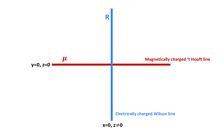
Figure 6: A magnetically charged ’t Hooft line crossing an electrical charged Wilson line. The two lines expands in the topological plane $\mathbb{R}^{2}$ of the 4D Chern-Simons theory.

8.2 Appendix B: Verma modules of $gl(m|n)$

The content of this appendix complements the study given in section 4. Representations of $gl(m|n)$ in $\mathbb{Z}_{2}$-graded vector space $V$ are Lie superalgebra homomorphisms $\varrho:gl(m|n)\rightarrow End(V)$ where the generators $\varrho\left(\mathcal{E}_{\text{{AB}}}\right)$ belonging to End($V$ ) obey the graded commutators (4.7). Below, we focus on the highest weight representations of $gl(m|n)$.

8.2.1 Highest weight representations

We begin by recalling that as for bosonic-like Lie algebras, a Verma module $M\left(\lambda\right):gl(m|n)\rightarrow End(V_{\lambda})$ is characterised by a highest weight vector $\lambda.$ By using the unit weight vector basis $\epsilon_{\text{{a}}},$ this highest weight can be expanded as follows [32]

$$\lambda=\sum_{\text{{a=1}}}^{m+n}\lambda_{\text{{a}}}\epsilon_{\text{{a}}}$$ (8.23)

where generally speaking the components $\lambda_{\text{{a}}}\in\mathbb{C}$. Below, we restrict to Verma modules with integral highest weights having integers $\lambda_{\text{{a}}}$ ordered like $\lambda_{\text{{a}}}\geq\lambda_{\text{{a+1}}}$ and moreover as

$$\lambda_{1}\geq\lambda_{2}\geq...\geq\lambda_{m}\geq 0\geq\lambda_{m+1}\geq...\geq\lambda_{m+n}$$ (8.24)

In practice, the highest weight representation $M\left(\lambda\right)$ can be built out of a highest-weight vector $\left|\Omega_{\lambda}\right\rangle$ (say the vacuum state) by acting on it by the $\mathcal{E}_{\text{{ab}}}$ generators of the superalgebra $End(V_{\lambda}).$ The $\left|\Omega_{\lambda}\right\rangle$ is an eigenstate of the diagonal operators $\mathcal{E}_{\text{{aa}}}$, and is annihilated by the step operators $\mathcal{E}_{\text{{ab}}}$ with a$<$b,

$$\mathcal{E}_{\text{{aa}}}\left|\Omega_{\lambda}\right\rangle$$ , a

,

(8.25)

Notice that the step operators $\mathcal{E}_{\text{{ab}}}$ are just the annihilation operators $\mathcal{E}_{+\beta_{\text{{ab}}}}$ associated with the positive roots $\beta_{\text{{ab}}}$. The other vectors in the $V_{\lambda}$ - module are obtained by acting on $\left|\Omega_{\lambda}\right\rangle$ by the creation operators as follows

$$\left|n_{1},...,n_{p}\right\rangle=\mathcal{E}_{-\mathrm{\gamma}_{1}}^{n_{1}}.....\mathcal{E}_{-\mathrm{\gamma}_{p}}^{n_{p}}\left|\Omega_{\lambda}\right\rangle\quad with\qquad n_{l}\in\left\{\begin{array}[]{ccc}\mathbb{N}\text{\ \ \ \ }&for&\deg n_{l}=0\\ \left\{0,1\right\}&for&\deg n_{l}=1\end{array}\right.$$ (8.26)

Here, the $\mathrm{\gamma}_{l}$’s stand for the positive roots $\beta_{\text{{ab}}}$ and the step operators $\mathcal{E}_{-\mathrm{\gamma}_{l}}^{n_{l}}$’s are the creation operators (lowering operators). The $\mathrm{\gamma}_{l}$’s expand in terms of the simple roots $\alpha_{\text{{a}}}=\epsilon_{\text{{a}}}-\epsilon_{\text{{a+1}}}$ as follows

$$\mathrm{\gamma}_{l}=\sum_{\text{{a}}}n_{l\text{{a}}}\alpha_{\text{{a}}}$$ (8.27)

with $n_{l\text{{a}}}$ some positive integers. Notice that two states $\left|n_{1},...,n_{p}\right\rangle$ and $\left|n_{1}^{\prime},...,n_{p}^{\prime}\right\rangle$ in $V_{\lambda}$ are identified if they are related by the super-commutation relations (4.7). Moreover, seen that the lowering operator $\mathcal{E}_{-\beta_{\text{{ab}}}}$ changes the highest weight $\lambda$ by the roots $-\beta_{\text{{ab}}}=-\left(\epsilon_{\text{{a}}}-\epsilon_{\text{{b}}}\right)$ (with a$<$b) we can determine the weight $\eta\left(\lambda\right)$ of the state

$$\left|\omega_{\eta\left(\lambda\right)}\right\rangle\equiv\left|n_{1},...,n_{p}\right\rangle$$ (8.28)

By using the simple roots $\alpha_{\text{{a}}}$ and the decomposition $\epsilon_{\text{{b}}}-\epsilon_{\text{{a}}}=\alpha_{\text{{b}}}+...+\alpha_{\text{{a-1}}},$ the weight $\eta$ of the state $\left|\omega_{\eta\left(\lambda\right)}\right\rangle$ has the form

$$\eta=\lambda-\sum_{\text{{a=1}}}^{m+n-1}M_{\text{{a}}}\alpha_{\text{{a}}}\qquad,\qquad M_{\text{{a}}}\in\mathbb{N}$$ (8.29)

We end this description by noticing that the Verma modules $M\left(\lambda\right)$ of the Lie superalgebra $gl\left(m|n\right)$ are infinite dimensional. However, for the particular case $\left(m|n\right)=\left(1|1\right)$, we have only one lowering operator $\mathcal{E}_{+\alpha}$ obeying the nilpotency property $\mathcal{E}_{+\alpha}^{2}=0$. As such, eq(8.26) reduces to

$$\left|l\right\rangle=\mathcal{E}_{-\mathrm{\alpha}}^{l}\left|\Omega_{\lambda}\right\rangle\qquad,\qquad l=0,1$$ (8.30)

with

$$\mathcal{E}_{\text{{11}}}\left|\Omega_{\lambda}\right\rangle$$

(8.31)

Recall that $gl\left(1|1\right)$ has four generators given by the two diagonal $\mathcal{E}_{\text{{11}}},\mathcal{E}_{\text{{22}}}$ and two odd step operators $\mathcal{E}_{\pm\alpha}$ corresponding to the roots $\pm\alpha=\pm\left(\varepsilon-\delta\right)$. A highest weight $\lambda$ of $gl\left(1|1\right)$ expands as $\lambda=\lambda_{1}\varepsilon+\lambda_{2}\delta$ and the Verma module $M\left(\lambda\right)$ associated with this $\lambda$ is generated by the two states namely

$$\left|\Omega_{\lambda}\right\rangle\qquad,\qquad\mathcal{E}_{-\mathrm{\alpha}}\left|\Omega_{\lambda}\right\rangle$$ (8.32)

8.2.2 Dynkin and Weight super- diagrams

Knowing the simple roots $\alpha_{\text{{a}}}=\epsilon_{\text{{a}}}-\epsilon_{\text{{a+1}}}$ of the Lie superalgebra $sl\left(m|n\right)$ and the highest weight $\lambda=\lambda_{\text{{a}}}\epsilon_{\text{{a}}}$ as well as the descendent $\eta=\lambda-M_{\text{{a}}}\alpha_{\text{{a}}}$ of a module $V_{\lambda},$ we can draw the content of the Dynkin graph of sl$\left(m|n\right)$ and the weight diagram of $V_{\lambda}$ in terms of quiver graphs. As roots and weights are expressed in terms of the unit weight vectors $\epsilon_{\text{{a}}}$, it is interesting to begin by representing the $\epsilon_{\text{{a}}}$’s. These $\epsilon_{\text{{a}}}$’s are represented by a vertical line. However, because of the two possible degrees of $\epsilon_{\text{{a}}}$, the vertical lines should be distinguished; they have different colors depending of the grading and are taken as:
$\left(i\right)$ red color for $\deg$a=0; that is for the real weight $\varepsilon_{a}$.
$\left(ii\right)$ blue color for $\deg$a=1, that is for the pure imaginary weight $\delta_{i}$.
So, we have the following building blocks for the $\epsilon_{\text{{a}}}$s,

$$\begin{array}[]{ccccccc}\varepsilon_{a}&:&{\color[rgb]{1,0,0}|}&\qquad,&\delta_{i}&:&{\color[rgb]{0,0,1}|}\end{array}$$ (8.33)

where we have used the splitting $\epsilon_{\text{{a}}}=\left(\varepsilon_{a},\delta_{i}\right)$.
Using these vertical lines, the ordered basis set $\left(\epsilon_{1},...,\epsilon_{m+n}\right)$ is then represented graphically by $m$ red vertical lines and n vertical blue lines placed in the order specified by the choice of the $\mathbb{Z}_{2}$-grading. For the example $gl\left(3|2\right)$ with basis set $\left(\varepsilon_{1},\varepsilon_{2},\delta_{1},\delta_{2},\varepsilon_{3}\right),$ we have the following graph

$$\varepsilon_{1}$$

(8.34)

The next step to do is to represent the roots and the weights. Simple roots $\alpha_{\text{{a}}}=\epsilon_{\text{{a}}}-\epsilon_{\text{{a+1}}}$ are represented by circle nodes $\bigcirc$ between each pair of adjacent vertical lines associated with $\epsilon_{\text{{a}}}$ and $\epsilon_{\text{{a+1}}}.$ For the previous example namely $sl\left(3|2\right)$ with basis set $\left(\varepsilon_{1},\varepsilon_{2},\delta_{1},\delta_{2},\varepsilon_{3}\right),$ we have

$$\alpha_{\text{{1}}}$$

(8.35)

$\bullet$ Super- Dynkin diagram
For each pair of simple roots $\left(\alpha_{\text{{a}}},\alpha_{\text{{b}}}\right)$ with non vanishing intersection matrix $K_{\text{{ab}}}=\alpha_{\text{{a}}}.\alpha_{\text{{b}}}\neq 0$, we draw an arrow from the a-th node to the b-th node. The $K_{\text{{ab}}}$ is an integer and written on the arrow. By hiding the vertical lines, we obtain the super- Dynkin diagram of $sl\left(m|n\right)$ with the specified basis $\left(\epsilon_{1},...,\epsilon_{m+n}\right)$. In the Figure 7, we give the super- Dynkin diagram of $sl\left(3|2\right)$ with weight basis as $\left(\varepsilon_{1},\varepsilon_{2},\delta_{1},\delta_{2},\varepsilon_{3}\right)$.

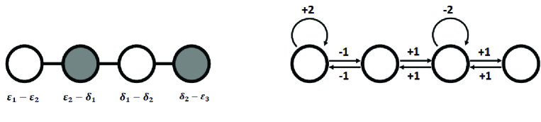
Figure 7: Building the Dynkin diagram of Lie superalgebra gl$\left(m|n\right).$ Here we give the example the Dynkin diagram of gl$\left(3|2\right)$ with weight basis ordered as $\left(\varepsilon_{1},\varepsilon_{2},\delta_{1},\delta_{2},\varepsilon_{3}\right).$ This graph is borrowed from [32].

Notice that the ordering is defined modulo the action of the Weyl group $W_{m}\times W_{n}$ which permutes the basis vectors $\left(\epsilon_{\text{{1}}},...,\epsilon_{\text{{m+n}}}\right)$ without changing the $\mathbb{Z}_{2}$-grading. For instance, the choice $\left(\varepsilon_{2},\varepsilon_{1},\delta_{1},\delta_{2},\varepsilon_{3}\right)$ leads to the same Dynkin diagram as the one given by the Figure 7.

$\bullet$ Super- weight diagrams
To represent the highest weight $\lambda=\lambda_{\text{{a}}}\epsilon_{\text{{a}}}$ of modules of the Lie superalgebra $gl\left(m|n\right)$, we first draw the (red and blue) vertical lines representing $\epsilon_{\text{{a}}}$ as in (8.34).
Then, for each vertical line representing $\epsilon_{\text{{a}}},$ we implement the coefficient $\lambda_{\text{{a}}}$ by drawing a diagonal line ending on the vertical $\epsilon_{\text{{a}}}$ and write $\lambda_{\text{{a}}}$ as in the Figure 8 illustrating highest weights

$$\lambda=\lambda_{\text{{1}}}\epsilon_{\text{{1}}}+\lambda_{\text{{2}}}\epsilon_{\text{{2}}}+\lambda_{\text{{3}}}\epsilon_{\text{{3}}}+\lambda_{\text{{4}}}\epsilon_{\text{{4}}}+\lambda_{\text{{5}}}\epsilon_{\text{{5}}}$$ (8.36)

in the Lie superalgebra $gl\left(3|2\right).$
To represent the weights $\eta=\lambda-M_{\text{{a}}}\alpha_{\text{{a}}}$ of the descendent states (8.26), we draw $M_{\text{{a}}}$ horizontal line segments between the a-th and $\left(\text{{a}}+1\right)$-st vertical lines. For the example of $gl\left(3|2\right)$ with basis set $\left(\varepsilon_{1},\varepsilon_{2},\delta_{1},\delta_{2},\varepsilon_{3}\right)$ and $\left(M_{1},M_{2},M_{3},M_{4}\right)=(2,3,2,1);$ that is

$$\eta=\lambda-2\alpha_{\text{{1}}}-3\alpha_{\text{{2}}}-2\alpha_{\text{{3}}}-\alpha_{\text{{4}}}$$ (8.37)

we have the weight diagram the Figure 8.

Figure 8: Building the weight diagram of representation of Lie superalgebra sl$\left(m|n\right).$ Here the diagram of the weight $\eta=\lambda-M_{\text{{a}}}\alpha_{\text{{a}}}$ in the Lie superalgebra gl$\left(3|2\right)$with $M_{\text{{a}}}$-integers as $\left(M_{1},M_{2},M_{3},M_{4}\right)=(2,3,2,1).$ This graph is borrowed from [32]. For generalisations and more information, we refer to this interesting study.

8.3 Appendix C: Derivation of eq(2.20) of ref.[29]

In this appendix, we give the explicit derivation of the Lax operator of eq(2.20) in ref.[29] obtained by Frassek, Lukowski, Meneghelli, Staudacher (FLMS solution). This solution was obtained by using the Yangian formalism; but here we show that we can derive it from the Chern-Simons theory with gauge super group family $SL(m|n)$ with $m\neq n$. For a recent description of these two formalisms (Yangian and Chern-Simons) applied to the bosonic like symmetries; see [61].
We begin by recalling that the FLMS solution was constructed in [29] for the Lie superalgebra $su(m|n)$, which naturally extends to its complexification $sl(m|n)$ that we are treating here. The L-operator obtained by FLMS has been presented as 2$\times 2$ matrix with entries given by matrix blocks that we present as follows

$$\mathcal{L}_{FLMS}=\left(\begin{array}[]{cc}L_{xy}&L_{x\dot{y}}\\ L_{\dot{x}y}&L_{\dot{x}\dot{y}}\end{array}\right)$$ (8.38)

where $x,\dot{x},y,\dot{y}$ are labels and where $L_{xy},L_{x\dot{y}},L_{\dot{x}y},L_{\dot{x}\dot{y}}$ are given by eq(2.20) in [29]; see also eq(8.55) derived below. So, in order to recover this solution from our analysis, we start from eq(6.5) of our paper that we can rewrite in condensed form as

$$\mathbf{\mu}_{p}$$

(8.39)

Here, we have set $\mathcal{P}_{1}=\Pi_{1}$ and $\mathcal{P}_{2}=\Pi_{2}+\Pi_{3}$ which are also projectors that satisfy the usual relations $\mathcal{P}_{k}.\mathcal{P}_{l}=\delta_{kl}\mathcal{P}_{k}$. The use of $\mathcal{P}_{1}$ and $\mathcal{P}_{2}$ instead of $\Pi_{1}$,$\Pi_{2},\Pi_{3}$ is to recover the 2$\times$2 representation (8.38). Using the bra-ket language and our label notations, we have $\mathcal{P}_{1}=\sum_{a=1}^{p}\left|a\right\rangle\left\langle a\right|$ and $\mathcal{P}_{2}=\sum_{A=p+1}^{m+n}\left|A\right\rangle\left\langle A\right|$ with matrix representations as follows

$$\mathcal{P}_{1}=\left(\begin{array}[]{cc}I_{{\small p\times p}}&0_{{\small p\times Q}}\\ 0_{{\small Q\times p}}&0_{{\small Q\times Q}}\end{array}\right),\qquad\mathcal{P}_{2}=\left(\begin{array}[]{cc}0_{{\small p\times p}}&0_{{\small p\times Q}}\\ 0_{{\small Q}\times p}&I_{{\small Q}\times{\small Q}}\end{array}\right)$$ (8.40)

where we have set ${\small Q=m+n-p}$. These projectors satisfy the usual identity resolution, namely $\mathcal{P}_{1}+\mathcal{P}_{2}=I_{\left(m+n\right)\times\left(m+n\right)}$.
Putting the expression (8.39) of $z^{\mathbf{\mu}_{p}}$ into the super L-operator $\mathcal{L}=e^{\Psi}z^{\mathbf{\mu}_{p}}e^{\Phi}$ given by eq(6.1), we end up with eqs(6.13-6.14) that read in terms of the projectors $\mathcal{P}_{1}$ and $\mathcal{P}_{2}$ as follows

$$\mathcal{L}$$

(8.41)

In this expression, $\Psi$ and $\Phi$ are valued in the nilpotent sub-superalgebras $\boldsymbol{N}_{+}$ and $\boldsymbol{N}_{-}$; they are given by (6.7-6.9). For convenience, we rewrite them in terms of super labels $\left(a,A\right)$ and $\left(b,B\right)$ as follows

$$\Psi=\sum_{a=1}^{p}\sum_{A=p+1}^{m+n}B^{aA}\mathbb{X}_{aA}\qquad,\qquad\Phi=\sum_{b=1}^{p}\sum_{B=p+1}^{m+n}C_{Bb}\mathbb{Y}^{Bb}$$ (8.42)

where $\mathbb{X}_{aA}$ and $\mathbb{Y}^{bA}$ are respectively the generators of the nilpotents $\boldsymbol{N}_{+}$ and $\boldsymbol{N}_{-}$. These graded generators are realised in terms of the canonical super states as follows

$$\mathbb{X}_{aA}=\left|a\right\rangle\left\langle A\right|\qquad,\qquad\mathbb{Y}^{Bb}=\left|B\right\rangle\left\langle b\right|$$ (8.43)

The coefficients $B^{aA}$ and $C_{Bb}$ are super Darboux coordinates of the phase space of the ’t Hooft super line; their canonical quantization, denoted like $\hat{B}^{aA}$ and $\hat{C}_{Bb},$ describe the associated quantum super oscillators. In matrix notation, the $B^{aA}$ and $C_{Bb}$ have the following form

$$B^{aA}=\left(\begin{array}[]{ccc}B^{1(p+1)}&\cdots&B^{1(m+n)}\\ \vdots&\ddots&\vdots\\ B^{p(p+1)}&\cdots&B^{p(m+n)}\end{array}\right)\qquad,\qquad C_{Bb}=\left(\begin{array}[]{ccc}C_{\left(p+1\right)1}&\cdots&C_{\left(p+1\right)p}\\ \vdots&\ddots&\vdots\\ C_{\left(m+n\right)1}&\cdots&C_{\left(m+n\right)p}\end{array}\right)$$ (8.44)

and similarly for the $\hat{B}^{aA}$ and $\hat{C}_{Bb}$ operators. For later use, notice that the product $\Psi\Phi$ reads as $\sum B^{aA}\mathbb{X}_{aA}\mathbb{Y}^{Bb}C_{Bb}$; by substituting the generators with their expressions (8.43), we obtain $\mathbb{X}_{aA}\mathbb{Y}^{Bb}=\delta_{A}^{B}\left|a\right\rangle\left\langle b\right|,$ and consequently

$$\Psi\Phi=\sum_{D}B^{aD}C_{Db}\left|a\right\rangle\left\langle b\right|$$ (8.45)

As far as this classical quantity is concerned, notice the three following interesting features:
$\left(\mathbf{1}\right)$ the product $\Psi\Phi$ can be expanded as $\sum_{D=p+1}^{m}b^{aD}c_{Db}+\sum_{D=m}^{m+n}\beta^{aD}\gamma_{Db},$ where the bosonic $b^{aD}$ and $c_{Db}$ as well as the fermionic $\beta^{aD}$ and $\gamma_{Db}$ are as in eqs(6.19-6.20).
$\left(\mathbf{2}\right)$ Classically speaking, the quadratic product $\Psi\Phi$ (8.45) can be also presented as follows

$$\Psi\Phi=\frac{1}{2}\sum_{D}\left(B^{aD}C_{Db}+\left(-\right)^{\left|D\right|}C_{Db}B^{aD}\right)\left|a\right\rangle\left\langle b\right|$$ (8.46)

just because the normal ordering is not required classically. The number $\left|D\right|$ refers here to the $\mathbb{Z}_{2}$-grading $0,1$. At the quantum level, the $\Psi$ and $\Phi$ are promoted to the operators $\hat{\Psi}$ and $\hat{\Phi}$; as such, the above product $\Psi\Phi$ must be replaced by the operator $\hat{\Psi}\hat{\Phi}$ which is given by the expansion

$$\hat{\Psi}\hat{\Phi}=\frac{1}{2}\sum_{D}\left(\hat{B}^{aD}\hat{C}_{Db}+\left(-\right)^{\left|D\right|}\hat{C}_{Db}\hat{B}^{aD}\right)\left|a\right\rangle\left\langle b\right|$$ (8.47)

Here, the graded commutators between the super oscillators $\hat{B}^{aA}$ and $\hat{C}_{Bb}$ are defined as usual by the super commutator $[\hat{C}_{Bb},\hat{B}^{aA}\}=\delta_{b}^{a}\delta_{B}^{A},$ which is a condensed form of eqs(6.21).
$\left(\mathbf{3}\right)$ From these super commutators, we learn that $\hat{C}_{Bb}\hat{B}^{aA}$ is given by $\delta_{b}^{a}\delta_{B}^{A}+\left(-\right)^{\left|A\right|\times\left|B\right|}\hat{B}^{aA}\hat{C}_{Bb}.$ Using this result, we can express $\left(-\right)^{\left|D\right|}\hat{C}_{Db}\hat{B}^{aD}$ as follows

$$\left(-\right)^{\left|D\right|}\hat{C}_{Db}\hat{B}^{aD}=\hat{B}^{aD}\hat{C}_{Db}+\left(-\right)^{\left|D\right|}\delta_{D}^{D}\delta_{b}^{a}$$ (8.48)

thus leading to

$$\hat{\Psi}\hat{\Phi}=\sum\limits_{D}\left(\hat{B}^{aD}\hat{C}_{Db}+\frac{1}{2}\left(-\right)^{\left|D\right|}\delta_{D}^{D}\delta_{b}^{a}\right)\left|a\right\rangle\left\langle b\right|$$ (8.49)

with $\frac{1}{2}\sum\limits_{D}\left(-\right)^{\left|D\right|}\delta_{D}^{D}$ given by

$$\frac{1}{2}\left(\sum\limits_{p+1}^{m}\left(-\right)^{\left|D\right|}\delta_{D}^{D}+\sum\limits_{m}^{m+n}\left(-\right)^{\left|D\right|}\delta_{D}^{D}\right)=\frac{1}{2}\left(m-p\right)-\frac{1}{2}n$$ (8.50)

Returning to the explicit calculation of (8.41), we use the useful properties $\Psi^{2}=0$ and $\Phi^{2}=0$, as well as

$$\Psi\mathcal{P}_{1}=0$$ , ,

, ,

(8.51)

So, eq(8.41) reduces to

$$\mathcal{L}$$

(8.52)

Using the properties (8.51), we obtain an expression in terms of the projectors $\mathcal{P}_{1}$ and $\mathcal{P}_{2}$ as well as $\mathcal{P}_{1}\Psi\Phi\mathcal{P}_{1},$ $\mathcal{P}_{1}\Psi\mathcal{P}_{2}$ and $\mathcal{P}_{2}\Phi\mathcal{P}_{1}$ that we present as follows

$$\mathcal{L}=\left(\begin{array}[]{cc}z^{1-\frac{p}{m-n}}\mathcal{P}_{1}+z^{-\frac{p}{m-n}}\mathcal{P}_{1}\Psi\Phi\mathcal{P}_{1}&z^{-\frac{p}{m-n}}\mathcal{P}_{1}\Psi\mathcal{P}_{2}\\ z^{-\frac{p}{m-n}}\mathcal{P}_{2}\Phi\mathcal{P}_{1}&z^{-\frac{p}{m-n}}\mathcal{P}_{2}\end{array}\right)$$ (8.53)

By multiplying by $z^{\frac{p}{m-n}}$ due to known properties of $\mathcal{L}$ as commented in the main text, we end up with the remarkable expression

$$\mathcal{L}=\left(\begin{array}[]{cc}z\mathcal{P}_{1}+\mathcal{P}_{1}\Psi\Phi\mathcal{P}_{1}&\mathcal{P}_{1}\Psi\mathcal{P}_{2}\\ \mathcal{P}_{2}\Phi\mathcal{P}_{1}&\mathcal{P}_{2}\end{array}\right)$$ (8.54)

Quantum mechanically, eq(8.54) is promoted to the hatted L-operator

$$\mathcal{\hat{L}}=\left(\begin{array}[]{cc}z\mathcal{P}_{1}+\mathcal{P}_{1}\hat{\Psi}\hat{\Phi}\mathcal{P}_{1}&\mathcal{P}_{1}\hat{\Psi}\mathcal{P}_{2}\\ \mathcal{P}_{2}\hat{\Phi}\mathcal{P}_{1}&\mathcal{P}_{2}\end{array}\right)$$ (8.55)

with $\hat{\Psi}\hat{\Phi}$ given by (8.49) which is precisely the FLMS solution obtained in [29].
We end this appendix by noticing that the present analysis can be extended to the families of Lie superalgebras listed in the table (4.1). This generalisation can be achieved by extending the bosonic construction done in [61] to supergroups including fermions. Progress in this direction will be reported in a future occasion.

References

- [1] K. Costello, E. Witten and M. Yamazaki, Gauge theory and integrability, I, ICCM Not. 6 (2018) 46, arXiv:1709.09993 [hep-th].
- [2] A. Kapustin, E. Witten, Electric-Magnetic Duality And The Geometric Langlands Program, High Energy Physics - Theory (hep-th), arXiv:hep-th/0604151.
- [3] Kazunobu Maruyoshi, Toshihiro Ota, Junya Yagi, Wilson-’t Hooft lines as transfer matrices, JHEP 01 (2021) 072, arXiv:2009.12391v2 [hep-th].
- [4] K. Maruyoshi, Wilson-’t Hooft Line Operators as Transfer Matrices. Progress of Theoretical and Experimental Physics, (2021).
- [5] Hirotaka Hayashi, Takuya Okuda, Yutaka Yoshida, ABCD of ’t Hooft operators, JHEP04(2021)241, arXiv:2012.12275v2 [hep-th].
- [6] Anton Kapustin, Natalia Saulina, The algebra of Wilson-’t Hooft operators, Nucl.Phys.B814:327-365,2009, arXiv:0710.2097 [hep-th].
- [7] Kapustin, A. Wilson-’t Hooft operators in four-dimensional gauge theories and S-duality. Physical Review D, 74(2), 025005, (2006), arXiv:hep-th/0501015.
- [8] K. Costello, E. Witten and M. Yamazaki, Gauge theory and integrability, II, ICCM Not. 6 (2018) 120 arXiv:1802.01579 [hep-th].
- [9] K. Costello, M. Yamazaki, Gauge Theory And Integrability, III, arXiv:1908.02289.
- [10] Y. Boujakhrout, E.H Saidi, R. Ahl Laamara, L.B Drissi, ’t Hooft lines of ADE-type and Topological Quivers, LPHE-MS preprint-2022, Under consideration in Physical Review D (2022).
- [11] Rachid Ahl Laamara, Lalla Btissam Drissi, El Hassan Saidi, D-string fluid in conifold: I. Topological gauge model, Nucl.Phys.B743:333-353,2006, arXiv:hep-th/0604001v1.
- [12] Rachid Ahl Laamara, Lalla Btissam Drissi, El Hassan Saidi, D-string fluid in conifold: II. Matrix model for D-droplets on S3 and S2, Nuclear Physics B 749(1):206-224, arXiv:hep-th/0605209v1.
- [13] K.Costello, D. Gaiotto, J.Yagi, Q-operators are ’t Hooft lines, arXiv:2103.01835 [hep-th], (2021).
- [14] E. Witten, Integrable Lattice Models From Gauge Theory, Advances in Theoretical and Mathematical Physics 21(7):1819-1843, arXiv:1611.00592 [hep-th].
- [15] Pronko, G. P. On Baxter’s Q-operator for the XXX spin chain. Communications in Mathematical Physics, 212(3), 687-701, (2000), arXiv:hep-th/9908179.
- [16] V.V. Bazhanov, R. Frassek, T. Łukowski, C. Meneghelli and M. Staudacher, Baxter Q-operators and Yangians, Nucl. Phys. B 850 (2011) 148, arXiv:1010.3699 [math-ph].
- [17] T. Okuda, Line operators in supersymmetric gauge theories. In New dualities of super gauge theories (pp. 195-222). Springer, (2016), arXiv:1412.7126 [hep-th].
- [18] R. Frassek, Oscillator realisations associated to the D-type Yangian: Nucl. Phys B, 956, 115063, (2020), arXiv:2001.06825 [math-ph].
- [19] Paul Ryan, Integrable systems, separation of variables and the Yang-Baxter equation, arXiv:2201.12057v1 [math-ph].
- [20] V. V. Bazhanov, T. Łukowski, C. Meneghelli, M.A Staudacher, shortcut to the Q-operator. Jour of Stat.Mechanics: Theory & Exp, 2010 (11), P11002, (2010).
- [21] M. Yamazaki, New Integrable Models from the Gauge/YBE Correspondence, arXiv:1307.1128 [hep-th].
- [22] Ilmar Gahramanov, Integrability from supersymmetric duality: a short review, arXiv:2201.00351 [hep-th].
- [23] E.H Saidi, Quantum line operators from Lax pairs, Journal of Mathematical Physics 61, 063501 (2020), arXiv:1812.06701 [hep-th].
- [24] N. Ishtiaque, S. F. Moosavian, Y. Zhou, Topological Holography: The Example of The D2-D4 Brane, System, arXiv:1809.00372 [hep-th].
- [25] Mykola Dedushenko and Davide Gaiotto, Correlators on the wall and sl spin chain, arXiv:2009.11198 [hep-th].
- [26] Bart Vlaar, Robert Weston, A Q-operator for open spin chains I: Baxter’s TQ relation, J. Phys. A: Math. Theor. 53 (2020) 245205, arXiv:2001.10760v2 [math-ph].
- [27] Gwenaël Ferrando, Rouven Frassek, Vladimir Kazakov, QQ-system and Weyl-type transfer matrices in integrable SO(2r) spin chains, JHEP02(2021)193, arXiv:2008.04336v3 [hep-th].
- [28] Kapustin, A. Wilson-’t Hooft operators in four-dimensional gauge theories and S-duality. Physical Review D, 74(2), 025005, (2006), arXiv:hep-th/0501015.
- [29] R. Frassek, T. Lukowski, C. Meneghelli, M. Staudacher, Oscillator Construction of Q-Operators, Nucl. Phys. B850 (2011) 175-198, arXiv:1012.6021 [math-ph].
- [30] B. H. Gross, On minuscule representations and the principal SL2. Represent. Theory, 4(200), arXiv:1509.04867 [math-ph] (2000).
- [31] Kac, V.G. (1977) Lie Superalgebras. Advances in Mathematics, 26, 8-96. http://dx.doi.org/10.1016/0001-8708(77)90017-2
- [32] N. Ishtiaque, S. F. Moosavian, S. Raghavendran, J. Yagi, Superspin chains from superstring theory, arXiv:2110.15112 [hep-th].
- [33] E.H Saidi, L.B Drissi, 5D N = 1 super QFT: symplectic quivers, Nucl Phys B 2021.
- [34] Meer Ashwinkumar, Meng-Chwan Tan, Unifying Lattice Models, Links and Quantum Geometric Langlands via Branes in String Theory, Adv.Theor.Math.Phys.24: 1681-1721, 2020, arXiv:1910.01134v3 [hep-th].
- [35] B. Charbonneau, J. Hurtubise, Singular Hermitian-Einstein monopoles on the product of a circle and a Riemann surface, arXiv:0812.0221 [math.DG].
- [36] J.P. Ang, Konstantinos Roumpedakis, Sahand Seifnashri, Line Operators of Gauge Theories on Non-Spin Manifolds, JHEP04(2020)087, arXiv:1911.00589v2 [hep-th].
- [37] Volker Schomerus and Hubert Saleur, The GL(11) WZW-Model: From Supergeometry to Logarithmic CFT, Nucl.Phys.B734:221-245,2006, arXiv:hep-th/0510032v1.
- [38] N. Aghaei, A.M. Gainutdinov, M. Pawelkiewicz, V. Schomerus, Combinatorial Quantisation of GL(11) Chern-Simons Theory I: The Torus, arXiv:1811.09123 [hep-th].
- [39] Y. Boujakhrout, E.H Saidi, On Exceptional ’t Hooft Lines in 4D-Chern-Simons Theory, Nuclear Physics B 2022, arXiv:2204.12424 [hep-th].
- [40] Robert H. Jonsson, Lucas Hackl, Krishanu Roychowdhury, Entanglement dualities in supersymmetry, Phys. Rev. Research 3, 023213 (2021), arXiv:2103.09657v2 [quant-ph].
- [41] V. Kazakov, S. Leurent and Z. Tsuboi, “Baxter’s Q-operators and operatorial Backlund flow for quantum (super)-spin chains,” Commun. Math. Phys. 311(2012) 787-814, [arXiv:1010.4022 [math-ph]].
- [42] L. Frappat, A. Sciarrino, P. Sorba, Dictionary on Lie Superalgebras, arXiv:hep-th/9607161v1.
- [43] Paolo Ciatti, Michael G. Cowling, The Levi Decomposition of a Graded Lie Algebra, arXiv:1705.06727v2.
- [44] Chih-Whi Chen, Shun-Jen Cheng, Kevin Coulembier, Tilting modules for classical Lie superalgebras, arXiv:1907.06579v1.
- [45] N. I. Stoilova, J. Van der Jeugt, Algebraic generalization of quantum statistics. Journal of Physics Conference Series (Online), 128(1), 13. doi:101088/1742-6596/128/1/012061.
- [46] Sergio L. Cacciatori, Bianca L. Cerchiai, Alessio Marrani, Magic coset decompositions, Adv. Theor. Math. Phys. 17(5): 1077-1128, 2013, arXiv:1201.6314 [hep-th].
- [47] R. B. Zhang, Serre presentations of Lie superalgebras, [arXiv:1101.3114, math.RT]
- [48] Victor Mikhaylov, Edward Witten, Branes And Supergroups, Communications in Mathematical Physics volume 340, pages 699–832 (2015), arXiv:1410.1175 [hep-th]
- [49] A. Mikovic, R. Picken, Super Chern Simons Theory and Flat Super Connections on a Torus, Adv.Theor.Math.Phys.5:243-263,2002, arXiv:math-ph/0008006.
- [50] L. B. Drissi, E. H. Saidi, Domain walls in topological tri-hinge matter, Eur. Phys. J. Plus (2021) 136: 68
- [51] L B Drissi, E H Saidi, A signature index for third order topological insulators, 2020 J. Phys.: Condens. Matter 32 365704.
- [52] A. P. Isaev, D. Karakhanyan, R. Kirschner, Yang-Baxter R-operators for osp superalgebras, Nuclear Physics B, 965, 2021, 115355 arXiv:2009.08143.
- [53] J. Fuksa, A. P. Isaev, D. Karakhanyan and R. Kirschner, Yangians and YangBaxter R-operators for ortho-symplectic superalgebras, Nucl. Phys. B 917 (2017) 44; [arXiv:1612.04713 [math-ph]].
- [54] J. Fuksa, A. P. Isaev, D. Karakhanyan and R. Kirschner, Yangians and Yang–Baxter R-operators for orthosymplectic superalgebras, Nucl. Phys. B 917, (2017) 44; arXiv:1612.04713 [math-ph].
- [55] A. P. Isaev, A. A. Provorov, The split Casimir operator and solutions of the Yang-Baxter equation for the osp(MN) and sl(MN) Lie superalgebras, arXiv:2201.06148 [math-ph].
- [56] E.H. Saidi, M.B. Sedra, HyperKhaler Metrics Building and Integrable Models, Mod.Phys.Lett. A9 (1994) 3163-3174, arXiv:hep-th/0512220v.
- [57] V. Caudrelier, E. Ragoucy, Lax pair and super-Yangian symmetry of the non-linear super-Schrödinger equation, J.Math.Phys. 44 (2003) 5706-5732, arXiv:math/0306115v1.
- [58] A. I. Molev, Representations of the super Yangians of types A and C, arXiv:2110.12784v1.
- [59] Kazunobu Maruyoshi, Junya Yagi, Surface defects as transfer matrices, Prog. Theor. Exp. Phys. (2016) 113B01, arXiv:1606.01041v3 [hep-th].
- [60] Hiroaki Kanno, Yuji Tachikawa, Instanton counting with a surface operator and the chain-saw quiver, JHEP 06 (2011) 119, arXiv:1105.0357v2 [hep-th].
- [61] Youssra Boujakhrout, El Hassan Saidi, Minuscule ABCDE Lax operators from 4D Chern-Simons theory, Nucl.Phys.B 981 (2022) 115859, arXiv:2207.14777v1 [hep-th].