Neutrino forces in neutrino backgrounds

Abstract

The Standard Model predicts a long-range force, proportional to $G_{F}^{2}/r^{5}$, between fermions due to the exchange of a pair of neutrinos. This quantum force is feeble and has not been observed yet. In this paper, we compute this force in the presence of neutrino backgrounds, both for isotropic and directional background neutrinos. We find that for the case of directional background the force can have a $1/r$ dependence and it can be significantly enhanced compared to the vacuum case. In particular, background effects caused by reactor, solar, and supernova neutrinos enhance the force by many orders of magnitude. The enhancement, however, occurs only in the direction parallel to the direction of the background neutrinos. We discuss the experimental prospects of detecting the neutrino force in neutrino backgrounds and find that the effect is close to the available sensitivity of the current fifth force experiments. Yet, the angular spread of the neutrino flux and that of the test masses reduce the strength of this force. The results are encouraging and a detailed experimental study is called for to check if the effect can be probed.

1 Introduction

It is well known that classical forces, like the Coulomb potential, can be derived from a $t$-channel mediator-exchange diagram in quantum field theory. The same treatment can be applied to the exchange of massive gauge bosons and scalars, resulting in a Yukawa potential. To obtain a classical force, the mediator of the force must be a boson. However, a pair of fermions behaves as an effective scalar and can mediate long-range forces. Such forces are sometimes called “quantum forces.” Quantum forces have been studied extensively in the literature, for example, see Hsu:1992tg ; Brax:2017xho ; Fichet:2017bng ; Costantino:2019ixl , in an attempt to both test the Standard Model (SM) and to probe new physics beyond.

In the SM, the force between fermions due to neutrino pair exchange is also well studied. Since neutrinos are very light, the force mediated by them is long range, without any significant exponential suppression with distance. Neutrino forces are generated by the exchange of a neutrino-antineutrino pair between two particles, as shown in the left panel of Fig. 1. The original idea of the neutrino-mediated force can be traced back to Feynman, who tried to explain the $1/r$ gravity as an emergent phenomenon due to the exchange of two neutrinos when taking into account multi-body effects Feynmangravitation . Previous calculations of such forces in vacuum were first carried out in Refs. Feinberg:1968zz ; Feinberg:1989ps ; Hsu:1992tg using the dispersion technique for massless neutrinos. Later, the effects of neutrino masses Grifols:1996fk and flavor mixing Lusignoli:2010gw ; LeThien:2019lxh ; Costantino:2020bei were included, which in principle can be used to determine the nature of neutrinos Segarra:2020rah ; Costantino:2020bei , namely, whether neutrinos are Dirac or Majorana particles. The study of neutrino forces in the framework of effective field theories was carried out in Ref. Bolton:2020xsm .

Neutrino forces have important cosmological and astrophysical effects, such as the stability of neutron stars Fischbach:1996qf ; Smirnov:1996vj ; Abada:1996nx ; Kachelriess:1997cr ; Kiers:1997ty ; Abada:1998ti ; Arafune:1998ft and the impact on dark matter in the early universe Orlofsky:2021mmy ; Coy:2022cpt . Recently, the calculation of neutrino forces went beyond the four-fermion contact interaction and a general formula describing the short-range behavior of neutrino forces was derived Xu:2021daf .

While theoretically we know that the force should be there, it has never been confirmed experimentally. The reason is that the force is very weak. The fact that it is second order in the weak interaction makes it proportional to $G_{F}^{2}$. In the limit of massless neutrinos, it is explicitly

$$V(r)\sim\frac{G_{F}^{2}}{r^{5}}\;,$$ (1)

where $G_{F}=1.166\times 10^{-5}{\rm GeV}^{-2}$ is the Fermi constant and $r$ is the distance between the two particles. Thus, already at distances longer than about a nanometer, the neutrino force is smaller than the gravitational force between elementary particles.

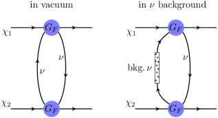
Figure 1: A diagrammatic explanation of neutrino forces in the vacuum (left) and in a neutrino background (right). The background effect can be taken into account by replacing one of the neutrino propagators with a background-modified propagator (bkg. $\nu$), which can be computed in finite temperature field theory. The effect can be physically interpreted as absorbing a neutrino from the background and then returning it back to the background.

Confirming the neutrino force experimentally would be interesting for several reasons. First, it would establish an exciting prediction of quantum field theory that remains untested. Second, it would enable us to probe the neutrino sector of the SM since the neutrino force is sensitive to the absolute masses of the neutrinos. Also, it provides a test of the electroweak interaction and may serve as a probe of new physics beyond the SM. Lastly, it would enable us to look for other quantum forces that may be present due to yet undiscovered light particles Grifols:1994zz ; Ferrer:1998ue ; Fichet:2017bng ; Brax:2017xho ; Costantino:2019ixl ; Banks:2020gpu .

Given that the neutrino force is so feeble, we need to look for novel ways to probe it. One such idea was put forward in Ghosh:2019dmi , which pointed out that the neutrino force provides the leading long-range parity-violation effect in the SM. Thus, it is natural to look for such effects. Yet even this seems too small to be probed experimentally.

In this paper, we explore a different path: the neutrino force in the presence of an intense neutrino background, as shown in the right panel of Fig. 1. The presence of the background can significantly increase the strength of the interaction. In fact, the effect of a neutrino background was studied before, for the cosmic neutrino background (C$\nu$B), in Refs. Horowitz:1993kw ; Ferrer:1998ju ; Ferrer:1999ad . However, the effect in this case is small because the number density of the cosmic neutrinos is very small today.

In this work, we focus on scenarios where the background is much more dense; in particular, for solar and reactor neutrinos. On the theoretical level, this differs from the case of C$\nu$B in that the background is not spherically symmetric. This results in a preferred direction, providing a fundamentally different signal than that of the vacuum and C$\nu$B cases.

Numerically, we find that the effect of reactor and solar neutrinos is remarkably significant and can enhance the signal by more than 20 orders of magnitude. In particular, the encouraging result is that the effect is close to the available sensitivity of fifth-force experimental searches. Thus, we hope that using the effect of background neutrinos will enable us to probe the neutrino force.

The paper is organized as follows. In Sec. 2, we set up the general formalism to calculate the neutrino force in an arbitrary neutrino background. After applying this formalism to the case of C$\nu$B in Sec. 3, we calculate the neutrino force in a directional neutrino flux background in Sec. 4. In Sec. 5, we discuss the detection of neutrino forces in neutrino backgrounds and compare our theoretical results with the experimental sensitivities. Our main conclusions are summarized in Sec. 6. The technical details are expanded in the appendices.

2 Formalism

In this section, we introduce the general formalism to compute neutrino forces between two fermions in a general neutrino background. Consider a four-fermion interaction with two Dirac neutrinos (for the case of Majorana neutrinos, see Sec. 3.3) and two fermions:

$${\cal L}_{{\rm int}}=-\frac{G_{F}}{\sqrt{2}}\left[\bar{\nu}\gamma^{\mu}\left(1-\gamma_{5}\right)\nu\right]\left[\bar{\chi}\gamma_{\mu}\left(g_{V}^{\chi}+g_{A}^{\chi}\gamma_{5}\right)\chi\right]\;,$$ (2)

where $G_{F}$ is the Fermi constant, $\nu$ denotes a Dirac neutrino with mass $m_{\nu}$, $\chi$ is a generic fermion in or beyond the SM with mass $m_{\chi}$, $g_{V}^{\chi}$ and $g_{A}^{\chi}$ are effective vector and axial couplings of $\chi$ to the neutrinos, obtained from integrating out heavy weak bosons.

Before we start, we note the following:

1. We work in the non-relativistic (NR) limit, i.e, the velocity of the interacting fermions $v\ll 1$ . The description of particle scattering via a potential $V(\mathbf{r})$ is accurate only in this limit.

2. Throughout our work, we only consider the spin-independent part of the potential. The reason is that the spin-dependent parts are usually averaged out when neutrino forces are added at macroscopic scales. The spin-independent part of the potential only depends on the vector coupling $g_{V}^{\chi}$. In Table 1, we collect the values of $g_{V}^{\chi}$ in the SM Giunti:2007ry . When $\chi$ is the proton or the neutron, $g_{V}^{\chi}$ can be obtained by simply summing over the vector couplings to the quarks.

In vacuum, the diagram in the left panel of Fig. 1 leads to a long-range force that we can describe by an effective potential proportional to $r^{-5}$ in the massless-neutrino limit, $r$ being the distance of the two external particles. More explicitly, the spin-independent part of the neutrino potential between two fermions $\chi_{1}$ and $\chi_{2}$ in that limit reads

$$V_{0}(r)=\frac{G_{F}^{2}g^{1}_{V}g^{2}_{V}}{4\pi^{3}}\frac{1}{r^{5}}\qquad(m_{\chi_{1,2}}^{-1}\ll r\ll m_{\nu}^{-1})\;.$$ (3)

Here, we use $g^{1}_{V}\equiv g^{\chi_{1}}_{V}$ and $g^{2}_{V}\equiv g^{\chi_{2}}_{V}$ to simplify the notation. Note that, for $r\gg 1/m_{\nu}$, the potential is exponentially suppressed by $e^{-2m_{\nu}r}$ Grifols:1996fk , while the NR approximation of $\chi$ becomes invalid as $r$ approaches $m_{\chi_{1,2}}^{-1}$. The short-range behavior of neutrino forces was first investigated in Ref. Xu:2021daf .

neutrino flavor	$\chi=e$	$\chi=u$	$\chi=d$	$\chi=$proton	$\chi=$neutron
$\nu_{e}$	$\frac{1}{2}+2s_{W}^{2}$	$\frac{1}{2}-\frac{4}{3}s_{W}^{2}$	$-\frac{1}{2}+\frac{2}{3}s_{W}^{2}$	$\frac{1}{2}-2s_{W}^{2}$	$-\frac{1}{2}$
$\nu_{\mu}$, $\nu_{\tau}$	$-\frac{1}{2}+2s_{W}^{2}$	$\frac{1}{2}-\frac{4}{3}s_{W}^{2}$	$-\frac{1}{2}+\frac{2}{3}s_{W}^{2}$	$\frac{1}{2}-2s_{W}^{2}$	$-\frac{1}{2}$

Table 1: Values of the vector coupling $g_{V}$ in Eq. (2) in the SM. Here $s_{W}\equiv\sin\theta_{W}$ is the sine of the Weinberg angle.

In a neutrino background with finite neutrino number density or temperature, the neutrino propagator should be modified, as shown on the right panel of Fig. 1. The modified propagator is often derived in the real-time formalism in finite temperature field theory (for a detailed review, see Refs. Landsman:1986uw ; Notzold:1987ik ; Quiros:1999jp ; Kapusta:2006pm ; Laine:2016hma . Also, see Appendix A for a simple and pedagogical re-derivation of the modified propagator.) We then have:

$$\!\!\!\!\!\!S_{\nu}(k)=\left(\not{k}+m_{\nu}\right)\left\{\frac{i}{k^{2}-m_{\nu}^{2}+i\epsilon}-2\pi\delta\left(k^{2}-m_{\nu}^{2}\right)\left[\Theta\left(k^{0}\right)n_{+}\left(\mathbf{k}\right)+\Theta\left(-k^{0}\right)n_{-}\left(\mathbf{k}\right)\right]\right\},$$ (4)

where $\epsilon\to 0^{+}$, $\Theta$ is the Heaviside theta function, and $n_{\pm}\left(\mathbf{k}\right)$ denote the momentum distributions of the neutrinos and anti-neutrinos respectively, such that the integrals $\int n_{\pm}\left(\mathbf{k}\right)d^{3}\mathbf{k}/(2\pi)^{3}$ correspond to their respective number densities. The first part is the usual fermion propagator in vacuum while the second part accounts for the background effect. The second part might seem counter-intuitive in the sense that the Dirac delta function requires the neutrino to be on-shell while, in Fig. 1, this on-shell neutrino is used to connect two spatially separated particles. To understand this effect, one should keep in mind that when $k$ in Eq. (4) is fixed, the uncertainty principle dictates that the neutrino cannot be localized and is spread out over space. So theoretically, the propagator’s second (background) term, just like the vacuum part, can mediate momentum over a large distance.

According to the Born approximation, the effective potential is the Fourier transform of the low-energy elastic scattering amplitude of $\chi_{1}$ with $\chi_{2}$,

$$V(\mathbf{r})=-\int\frac{d^{3}\mathbf{q}}{\left(2\pi\right)^{3}}e^{i\mathbf{q}\cdot\mathbf{r}}{\cal A}(\mathbf{q})\thinspace.$$ (5)

Here, ${\cal A}(\mathbf{q})$ is the scattering amplitude in the NR limit, which should be computed by integrating the neutrino loop in Fig. 1 using the modified neutrino propagator in Eq. (4):

$$i{\cal A}(q)=\frac{G_{F}^{2}g^{1}_{V}g^{2}_{V}}{2}\int\frac{d^{4}k}{\left(2\pi\right)^{4}}{\rm Tr}\left[\gamma^{0}\left(1-\gamma_{5}\right)S_{\nu}(k)\gamma^{0}\left(1-\gamma_{5}\right)S_{\nu}\left(k+q\right)\right].$$ (6)

Using the NR approximation we have $q\approx(0,\mathbf{q})$, thus the amplitude ${\cal A}$ only depends on the three-momentum $\mathbf{q}$. Substituting Eq. (4) into Eq. (6), one can see that when both neutrino propagators in Eq. (6) take the first term in the curly bracket of Eq. (4), it leads to the vacuum potential $V_{0}(r)$. When both propagators take the second term, the result vanishes, as we show in Appendix B. The background effect comes from cross terms, being proportional to $n_{\pm}$. We denote the background contribution to ${\cal A}(\mathbf{q})$ by ${\cal A}_{{\rm bkg}}(\mathbf{q})$ and, correspondingly, the contribution to $V(\mathbf{r})$ by $V_{{\rm bkg}}(\mathbf{r})$:

$${\cal A}(\mathbf{q})={\cal A}_{0}(\mathbf{q})+{\cal A}_{{\rm bkg}}(\mathbf{q})\thinspace,\qquad V(\mathbf{r})=V_{0}(\mathbf{r})+V_{{\rm bkg}}(\mathbf{r})\thinspace.$$ (7)

Notice that there is no interference between the vacuum and the background amplitudes in our calculation because, unlike computing cross sections, here we do not need to square the total amplitude. The background contribution ${\cal A}_{{\rm bkg}}(\mathbf{q})$, after some calculations in Appendix B, reduces to

$${\cal A}_{{\rm bkg}}(\mathbf{q})=4G_{F}^{2}g^{1}_{V}g^{2}_{V}\int\frac{d^{3}\mathbf{k}}{\left(2\pi\right)^{3}}\frac{n_{+}\left(\mathbf{k}\right)+n_{-}\left(\mathbf{k}\right)}{2E_{k}}\left[\frac{2\left|\mathbf{k}\right|^{2}+m_{\nu}^{2}+\mathbf{k}\cdot\mathbf{q}}{2\mathbf{k}\cdot\mathbf{q}+\left|\mathbf{q}\right|^{2}}+\left(\mathbf{k}\to-\mathbf{k}\right)\right].$$ (8)

For isotropic distributions (e.g. cosmic neutrino background, diffuse supernova neutrino background), $n_{\pm}$ are independent of the direction of the momentum, i.e., $n_{\pm}(\mathbf{k})=n_{\pm}(\kappa)$ with $\kappa\equiv\left|\mathbf{k}\right|$, leading to an isotropic ${\cal A}_{{\rm bkg}}$ and hence an isotropic $V_{{\rm bkg}}$. In this case, the angular part of the above integral can be integrated out analytically, resulting in the following expression for $V_{{\rm bkg}}$:

$$V_{{\rm bkg}}(r)=-\frac{G_{F}^{2}g^{1}_{V}g^{2}_{V}}{4\pi^{3}r^{4}}\int_{0}^{\infty}d\kappa\,\kappa\,\frac{n_{+}\left(\kappa\right)+n_{-}\left(\kappa\right)}{\sqrt{\kappa^{2}+m_{\nu}^{2}}}\left[\left(1+m_{\nu}^{2}r^{2}\right)\sin\left(2\kappa r\right)-2\kappa r\cos\left(2\kappa r\right)\right].$$ (9)

Up to now, we have not used any specific neutrino distributions. In what follows, we apply the above formulae to specific forms of $n_{\pm}$ and compute the corresponding potentials.

3 Neutrino forces with isotropic neutrino background

We now discuss the case where the neutrino background is isotropic and focus on a thermal-like distribution. In particular, this applies to the cosmic neutrino background (C$\nu$B), which motivates this section.

The existence of isotropic C$\nu$B today, with a temperature around 1.9 K and number density about $56/{\rm cm}^{3}$ per flavor, is one of the most solid predictions from big bang cosmology  Weinberg2008cosmology . The temperature correction to neutrino forces in the C$\nu$B was first calculated in Ref. Horowitz:1993kw with the neutrino momentum distribution to be

$$n_{\pm}\left(\mathbf{k},T\right)={\rm exp}\left[\left(\pm\mu-\kappa\right)/T\right]\quad{\rm with}\quad\kappa\equiv\left|\mathbf{k}\right|\;,$$ (10)

where $\mu$ and $T$ are the chemical potential and temperature of the C$\nu$B.

Ref. Horowitz:1993kw studied the case of Dirac neutrinos in the massless ($m_{\nu}=0$) and NR ($m_{\nu}\gg T$) limit. Later, the background effects of the C$\nu$B on neutrino forces were further studied in Ref. Ferrer:1998ju ; Ferrer:1999ad . In Ref. Ferrer:1998ju the neutrino distribution was taken to be a standard Boltzmann distribution,

$$n_{\pm}\left(\mathbf{k},T\right)={\rm exp}\left[\left(\pm\mu-E_{k}\right)/T\right]\quad{\rm with}\quad E_{k}=\sqrt{\left|\mathbf{k}\right|^{2}+m_{\nu}^{2}}\;,$$ (11)

and the complete expressions of the background potential $V_{\rm bkg}(r)$ were given for both Dirac and Majorana neutrinos. The massless limit of the result in Ref. Ferrer:1998ju matches that in Ref. Horowitz:1993kw . However, the results of the massive case are very different. In particular, the expression of $V_{\rm bkg}(r)$ in Ref. Ferrer:1998ju is exponentially suppressed at large distances, $V_{\rm bkg}(r)\sim e^{-2m_{\nu}r}$ (for $r\gg 1/m_{\nu}$), while that in Ref. Horowitz:1993kw is not, $V_{\rm bkg}(r)\sim m_{\nu}/(Tr^{5})$ (for $r\gg 1/T\gg 1/m_{\nu}$). This discrepancy on the long-range behavior of $V_{\rm bkg}(r)$ is due to the difference between the distributions in Eqs. (10) and (11): The former corresponds to the number density of relic neutrinos proportional to $T^{3}$, while the latter distribution corresponds to the number density that would be exponentially suppressed by $e^{-m_{\nu}/T}$ for NR neutrinos. In addition, in Ref. Ferrer:1999ad , $V_{\rm bkg}(r)$ was calculated for the standard Fermi-Dirac distribution

$$n_{\pm}\left(\mathbf{k},T\right)=\frac{1}{e^{\left(E_{k}\mp\mu\right)/T}+1}\;,$$ (12)

for arbitrary chemical potential, but the mass of neutrinos was neglected therein.

However, in the framework of standard cosmology, neutrinos decoupled at $T\sim{\rm MeV}$, after which they were no longer in thermal equilibrium with the cosmic plasma. Instead, they propagated freely until today, maintaining their own distribution:

$$n_{\pm}\left(\mathbf{k},T\right)=\frac{1}{e^{\left(\kappa\mp\mu\right)/T}+1}\;.$$ (13)

The reason why cosmic neutrinos obey the distribution function in Eq. (13), instead of Eq. (12), is that $\kappa$, rather than $E_{k}$, scales as inversely proportional to the scale factor $a$, i.e., $\kappa\propto 1/a$ Weinberg2008cosmology . In the relativistic limit, there is no difference between Eqs. (12) and (13). However, we know that the temperature of C$\nu$B today is around $10^{-4}$ eV and neutrino oscillation experiments Esteban:2020cvm tell us that at least two of the three active neutrinos are NR in the C$\nu$B today. Therefore, the results in Refs. Ferrer:1998ju ; Ferrer:1999ad using Eqs. (11) and (12) only hold for relativistic neutrino background and are invalid for the C$\nu$B today, while the computation in Ref. Horowitz:1993kw using Eq. (10) is an approximate result.

We emphasize that a strict computation of the background effects on neutrino forces from the C$\nu$B today using Eq. (13) is still lacking, and this is what we do in this section.

3.1 Maxwell-Boltzmann distribution

As a warm-up, we first take the distribution function in Eq. (10), whose massless and NR limits have already been given in Ref. Horowitz:1993kw . Substituting

$$n_{+}\left(\mathbf{k},T\right)+n_{-}\left(\mathbf{k},T\right)=2\cosh\left(\frac{\mu}{T}\right)\exp\left(-\frac{\kappa}{T}\right)\;,$$ (14)

into Eq. (9), we obtain

$$V_{\rm bkg}(r)=-\frac{G_{F}^{2}g^{1}_{V}g^{2}_{V}}{2\pi^{3}}\cosh\left(\frac{\mu}{T}\right)\frac{T}{r^{4}}\left[\left(1+b^{2}x^{2}\right){\cal I}_{\rm MB}\left(x,b\right)-b\frac{\partial}{\partial b}{\cal I}_{\rm MB}\left(x,b\right)\right]C_{\rm L}(T)\;,$$ (15)

where we have defined the dimensionless quantities

$$x\equiv\frac{m_{\nu}}{T},\qquad b\equiv rT,\qquad y\equiv\frac{\kappa}{T}\;,$$ (16)

with

$$C_{\rm L}(T)=\frac{1}{2}\left(1+\frac{p_{\nu}}{E_{\nu}+m_{\nu}}\right),$$ (17)

and the dimensionless integral

$${\cal I}_{\rm MB}(x,b)=\int_{0}^{\infty}dy\frac{y}{\sqrt{y^{2}+x^{2}}}e^{-y}\sin\left(2by\right)\;.$$ (18)

The factor $C_{\rm L}(T)$ in Eq. (15) accounts for the effect of chiral projection of the cosmic background neutrinos into their active component. Here, $E_{\nu}$ is the average energy and $p_{\nu}$ is the momentum, and they both depend on the temperature. Note that the modified propagator in Eq. (4) is valid for a general 4-component Dirac spinor. However, in C$\nu$B, only left-handed (LH) chiral neutrinos will contribute to the background force. When cosmic neutrinos are at freeze-out, they are ultra-relativistic and LH helicity state. As the temperature decreases, the mass of the Dirac neutrinos will lead to a population of the right-handed (RH) ones that are sterile to the background force. That is, the factor $C_{\rm L}(T)$ is the amount of LH chiral component in an LH helicity state. It is obvious that $C_{\rm L}=1$ in the massless limit while $C_{\rm L}=1/2$ in the NR limit, which corresponds to the fact that only half of the initial LH helicity neutrinos become LH chiral state when they are non-relativistic.

Eq. (18) cannot be integrated analytically but can be computed numerically for arbitrary values of $m_{\nu}$, $T$ and $r$. We are mainly interested in two special scenarios: $x=0$ (the lightest active neutrino can still be massless) and $x\gg 1$ (according to the neutrino oscillation experiments, the heaviest active neutrino is at least 0.05 eV, which corresponds to $x\gtrsim 500$ if we consider the temperature of C$\nu$B).

For $x=0$, we have

$${\cal I}_{\rm MB}\left(0,b\right)=\frac{2b}{1+4b^{2}}=\frac{2rT}{1+4r^{2}T^{2}}\;,$$ (19)

and

$$V_{\rm bkg}(r)=-\frac{8G_{F}^{2}g^{1}_{V}g^{2}_{V}}{\pi^{3}}\cosh\left(\frac{\mu}{T}\right)\frac{T^{4}}{r\left(1+4r^{2}T^{2}\right)^{2}}\qquad(m_{\nu}=0)\;,$$ (20)

which is consistent with the result in Refs. Horowitz:1993kw ; Ferrer:1998ju . In particular, for high temperatures, $r\gg 1/T$, we notice that $V_{T}(r)\sim 1/r^{5}$, which is almost independent of the temperature. For low temperature, $r\ll 1/T$, we find that $V_{T}(r)\sim T^{4}/r$.

For $x\gg 1$, since the integral in Eq. (18) with $y>1$ is exponentially suppressed, the dominant contribution to the integral comes from the region $0<y\ll x$, thus we have

$${\cal I}_{\rm MB}\left(x,b\right)\simeq\frac{1}{x}\int_{0}^{\infty}dyye^{-y}\sin\left(2by\right)=\frac{1}{x}\frac{4b}{\left(1+4b^{2}\right)^{2}}=\frac{4rT^{2}}{m\left(1+4r^{2}T^{2}\right)^{2}}\;,$$ (21)

and

$$V_{\rm bkg}(r)=-\frac{G_{F}^{2}g^{1}_{V}g^{2}_{V}}{\pi^{3}}\cosh\left(\frac{\mu}{T}\right)\frac{m_{\nu}T^{3}}{r\left(1+4r^{2}T^{2}\right)^{2}}\qquad(m_{\nu}\gg T)\;.$$ (22)

Note that, in contrast to the result in Ref. Ferrer:1998ju , there is no exponential suppression in Eq. (22). In particular, for $r\ll 1/T$, we obtain

$$V_{\rm bkg}(r)=-\frac{G_{F}^{2}g^{1}_{V}g^{2}_{V}}{\pi^{3}}\cosh\left(\frac{\mu}{T}\right)\frac{m_{\nu}T^{3}}{r}\qquad(m_{\nu}\gg T,\;\;r\ll T^{-1})\;,$$ (23)

while, for $r\gg 1/T$,

$$V_{\rm bkg}(r)=-\frac{G_{F}^{2}g^{1}_{V}g^{2}_{V}}{16\pi^{3}}\cosh\left(\frac{\mu}{T}\right)\frac{m_{\nu}}{T}\frac{1}{r^{5}}\qquad\left(m_{\nu}\gg T,\;\;r\gg T^{-1}\right)\;,$$ (24)

which is enhanced by a factor of $m_{\nu}/T$ compared with the vacuum result in Eq. (3) for NR background neutrinos.

3.2 Fermi-Dirac distribution

We now turn to the realistic distribution of background neutrinos in Eq. (13). The first thing to notice is that the neutrino degeneracy parameter $\zeta\equiv\mu/T$, which characterizes the neutrino–antineutrino asymmetry, is actually very small from constraints of big bang nucleosynthesis: $\zeta\lesssim{\cal O}\left(10^{-2}\right)$ Serpico:2005bc ; Lesgourgues:2006nd . Therefore, we can expand the neutrino distribution function into a series of $\zeta$,

$$n_{+}\left(\mathbf{\kappa},T\right)+n_{-}\left(\mathbf{\kappa},T\right)=\frac{2}{e^{\kappa/T}+1}+{\cal O}\left(\zeta^{2}\right)\;,$$ (25)

and only take the leading-order term, which is independent of $\zeta$. Then the background potential turns out to be

$$V_{\rm bkg}(r)=-\frac{G_{F}^{2}g^{1}_{V}g^{2}_{V}}{2\pi^{3}}\frac{T}{r^{4}}\left[\left(1+b^{2}x^{2}\right){\cal I}_{\rm FD}\left(x,b\right)-b\frac{\partial}{\partial b}{\cal I}_{\rm FD}\left(x,b\right)\right]C_{\rm L}(T)\;,$$ (26)

where $x$, $b$, and $y$ are defined in Eq. (16) and

$${\cal I}_{\rm FD}\left(x,b\right)=\int_{0}^{\infty}dy\frac{y}{\sqrt{y^{2}+x^{2}}}\frac{1}{e^{y}+1}\sin\left(2b\,y\right)\;.$$ (27)

The integral in Eq. (27) can be numerically calculated for arbitrary values of $m_{\nu}$, $T$, and $r$. In the massless limit $(x=0)$ and NR limit $(x\gg 1)$, ${\cal I}_{\rm FD}\left(x,b\right)$ can be carried out analytically.

For $x=0$, we have

$${\cal I}_{\rm FD}\left(x,b\right)=\frac{1}{4}\left[\frac{1}{b}-2\pi\,{\rm csch}\left(2\pi b\right)\right]\;,$$ (28)

and the background potential

$$V_{\rm bkg}(r)=-\frac{G_{F}^{2}g^{1}_{V}g^{2}_{V}}{4\pi^{3}}\frac{1}{r^{5}}\left\{1-\pi rT{\rm csch}\left(2\pi rT\right)\left[1+2\pi rT{\rm coth}\left(2\pi rT\right)\right]\right\}\quad(m_{\nu}=0)\;,$$ (29)

which is consistent with the result obtained in Ref. Ferrer:1999ad , where the neutrino distribution Eq. (12) was taken but the neutrino mass was neglected. An interesting observation is that, in the long-range limit,

$$V_{\rm bkg}(r)=-\frac{G_{F}^{2}g^{1}_{V}g^{2}_{V}}{4\pi^{3}}\frac{1}{r^{5}}\qquad(m_{\nu}=0,\;\;r\gg T^{-1})\;,$$ (30)

which happens to be the opposite of Eq. (3). This means that, for massless neutrinos in the limit $\zeta\to 0$, the vacuum potential is completely screened off by the C$\nu$B.

$\nu$BDF	$m_{\nu}=0$, $r\ll T^{-1}$	$m_{\nu}=0$, $r\gg T^{-1}$	$m_{\nu}\gg T$, $r\ll T^{-1}$	$m_{\nu}\gg T$, $r\gg T^{-1}$
MB	$-\frac{8}{\pi^{3}}G_{F}^{2}g^{1}_{V}g^{2}_{V}\frac{T^{4}}{r}$	$-\frac{1}{2\pi^{3}}G_{F}^{2}g^{1}_{V}g^{2}_{V}\frac{1}{r^{5}}$	$-\frac{1}{\pi^{3}}G_{F}^{2}g^{1}_{V}g^{2}_{V}\frac{m_{\nu}T^{3}}{r}$	$-\frac{1}{16\pi^{3}}G_{F}^{2}g^{1}_{V}g^{2}_{V}\frac{m_{\nu}}{T}\frac{1}{r^{5}}$
FD	$-\frac{7\pi}{90}G_{F}^{2}g^{1}_{V}g^{2}_{V}\frac{T^{4}}{r}$	$-\frac{1}{4\pi^{3}}G_{F}^{2}g^{1}_{V}g^{2}_{V}\frac{1}{r^{5}}$	$-\frac{3\zeta(3)}{4\pi^{3}}G_{F}^{2}g^{1}_{V}g^{2}_{V}\frac{m_{\nu}T^{3}}{r}$	$-\frac{1}{64\pi^{3}}G_{F}^{2}g^{1}_{V}g^{2}_{V}\frac{m_{\nu}}{T}\frac{1}{r^{5}}$

Table 2: Comparison of the short- and long-range behaviors of the background potential $V_{\rm bkg}(r)$ in the massless and non-relativistic limits with the neutrino Background Distribution Function ($\nu$BDF) taking the Maxwell-Boltzmann (MB) distribution in Eq. (10) and Fermi-Dirac (FD) distribution in Eq. (13). We have neglected the chemical potential in both distribution functions.

Let us now take a look at the NR limit of Eq. (27). As with the case of Boltzmann distribution, for $x\gg 1$, one obtains

$${\cal I}_{\rm FD}\left(x,b\right) \simeq \frac{1}{x}\int_{0}^{\infty}dy\frac{y}{e^{y}+1}\sin\left(2by\right)$$ (31)

$$= \frac{i}{8x}\left[\psi^{(1)}\left(\frac{1}{2}+ib\right)-\psi^{(1)}\left(\frac{1}{2}-ib\right)+\psi^{(1)}\left(1-ib\right)-\psi^{(1)}\left(1+ib\right)\right],$$

where the $n$-th ordered polygamma function is defined as

$$\psi^{(n)}(z)=\frac{d}{dz}\psi^{(n-1)}(z)=\frac{d^{n+1}}{dz^{n+1}}\log\Gamma(z)\;,$$ (32)

with $\Gamma(z)$ being the gamma function. Therefore, the background potential of NR cosmic neutrinos turns out to be

$$V_{\rm bkg}(r) = -i\frac{G_{F}^{2}g^{1}_{V}g^{2}_{V}}{32\pi^{3}}\frac{T^{2}}{mr^{4}}\left\{\left[\psi^{(1)}\left(\frac{1}{2}+ib\right)-\psi^{(1)}\left(\frac{1}{2}-ib\right)+\psi^{(1)}\left(1-ib\right)-\psi^{(1)}\left(1+ib\right)\right]\right.$$ (33)

$$\times \left.\left(1+b^{2}x^{2}\right)-ib\left[\psi^{(2)}\left(\frac{1}{2}+ib\right)+\psi^{(2)}\left(\frac{1}{2}-ib\right)-\psi^{(2)}\left(1-ib\right)-\psi^{(2)}\left(1+ib\right)\right]\right\},$$

$$\qquad\qquad\qquad\qquad\qquad\qquad\qquad\qquad\qquad\qquad\qquad\qquad\qquad(m_{\nu}\gg T)$$

In particular, for $r\ll 1/T$, i.e., $b\ll 1$, we have

$$V_{\rm bkg}(r) = -\left[\psi^{(2)}(1)-\psi^{(2)}\left(\frac{1}{2}\right)\right]\frac{G_{F}^{2}g^{1}_{V}g_{V}^{2}}{16\pi^{3}}\frac{m_{\nu}T^{3}}{r}$$ (34)

$$= -\frac{3\zeta(3)}{4\pi^{3}}G_{F}^{2}g^{1}_{V}g^{2}_{V}\frac{m_{\nu}T^{3}}{r}\qquad\left(m_{\nu}\gg T,\;\;r\ll T^{-1}\right),$$

with $\zeta(3)\simeq 1.202$ the Riemann zeta function, while, for the long-range limit $b\gg 1$, one obtains

$$V_{\rm bkg}(r)=-\frac{G_{F}^{2}g^{1}_{V}g^{2}_{V}}{64\pi^{3}}\frac{m_{\nu}}{T}\frac{1}{r^{5}}\qquad\left(m_{\nu}\gg T,\;\;r\gg T^{-1}\right),$$ (35)

which is, as in the case of the Boltzmann distribution, enhanced by a factor of $m_{\nu}/T$ compared with the vacuum potential in Eq. (3).

To sum up, we have provided in Eq. (26) the general background potential valid for any temperatures and distances and discussed the special scenarios in the massless and NR neutrinos limits, which have simple analytical expressions. Compared to the results of Maxwell-Boltzmann distribution in last subsection, we conclude that both distributions lead to similar short-range and long-range behaviors of the background potential in the massless limit ($m_{\nu}=0$) and NR limit ($m_{\nu}\gg T$), up to some numerical factors (cf. Table 2).

3.3 The case of Majorana neutrinos

The above calculations for Dirac neutrinos can be generalized to the scenario of Majorana neutrinos. If $\nu$ is a Majorana neutrino with mass $m_{\nu}$, then its general four-fermion interaction is given by

$${\cal L}_{\rm int}=\frac{G_{F}}{\sqrt{2}}\left[\bar{\nu}\gamma^{\mu}\gamma_{5}\nu\right]\left[\bar{\chi}\gamma_{\mu}\left(g_{V}^{\chi}+g_{A}^{\chi}\gamma_{5}\right)\chi\right]\;,$$ (36)

where we have used the identity $\bar{\nu}\gamma^{\mu}\nu=0$ for Majorana fermions comparing with Eq. (2). Taking into account the modified neutrino propagator due to the background, Eq. (4), the scattering amplitude reads

$$i{\cal A}(q)=\frac{G_{F}^{2}g^{1}_{V}g^{2}_{V}}{2}\int\frac{d^{4}k}{\left(2\pi\right)^{4}}{\rm Tr}\left[\gamma^{0}\gamma_{5}S_{\nu}(k)\gamma^{0}\gamma_{5}S_{\nu}\left(k+q\right)\right]\times 2\;,$$ (37)

where the factor of 2 is due to the exchange of two neutrino propagators in the loop. As with the Dirac case, the background effect comes from the crossed terms. After some algebra, one obtains

$${\cal A}_{{\rm bkg}}(\mathbf{q})=4G_{F}^{2}g^{1}_{V}g^{2}_{V}\int\frac{d^{3}\mathbf{k}}{\left(2\pi\right)^{3}}\frac{n_{+}\left(\mathbf{k}\right)+n_{-}\left(\mathbf{k}\right)}{2E_{k}}\left[\frac{2\left|\mathbf{k}\right|^{2}+\mathbf{k}\cdot\mathbf{q}}{2\mathbf{k}\cdot\mathbf{q}+\left|\mathbf{q}\right|^{2}}+\left(\mathbf{k}\to-\mathbf{k}\right)\right].$$ (38)

For isotropic distributions $n_{\pm}(\mathbf{k})=n_{\pm}(\kappa)$, Eq. (38) can be reduced to

$$V_{{\rm bkg}}(r)=-\frac{G_{F}^{2}g^{1}_{V}g^{2}_{V}}{4\pi^{3}r^{4}}\int_{0}^{\infty}d\kappa\,\kappa\,\frac{n_{+}\left(\kappa\right)+n_{-}\left(\kappa\right)}{\sqrt{\kappa^{2}+m_{\nu}^{2}}}\left[\sin\left(2\kappa r\right)-2\kappa r\cos\left(2\kappa r\right)\right]\;,$$ (39)

which, as expected, matches the result for Dirac neutrinos in Eq. (9) in the massless limit.

We then take the Fermi-Dirac distribution in Eq. (13) to calculate $V_{{\rm bkg}}(r)$ in the C$\nu$B. Note that for Majorana neutrinos, the chemical potential vanishes, so that

$$n_{+}(\kappa)=n_{-}(\kappa)=\frac{1}{e^{\kappa/T}+1}\;.$$ (40)

Therefore, the background potential turns out to be

$$V_{\rm bkg}(r)=-\frac{G_{F}^{2}g^{1}_{V}g^{2}_{V}}{2\pi^{3}}\frac{T}{r^{4}}\left[{\cal I}_{\rm FD}\left(x,b\right)-b\frac{\partial}{\partial b}{\cal I}_{\rm FD}\left(x,b\right)\right]\;,$$ (41)

where $x$, $b$, and the integral ${\cal I}_{\rm FD}(x,b)$ is defined in Eqs. (16) and (27). Note that for Majorana neutrinos, there is no need to include the factor of chiral projection (17) as the Dirac neutrino case.

In the massless limit ($x=0$), it is obvious that $V_{\rm bkg}(r)$ is the same as we have for the Dirac neutrino case in Eq. (29).

In the NR limit ($x\gg 1$), ${\cal I}_{\rm FD}(x,b)$ can be integrated analytically and is given by Eq. (31). Therefore the background potential turns out to be

$$V_{\rm bkg}(r) = -i\frac{G_{F}^{2}g^{1}_{V}g^{2}_{V}}{16\pi^{3}}\frac{T^{2}}{mr^{4}}\left\{\left[\psi^{(1)}\left(\frac{1}{2}+ib\right)-\psi^{(1)}\left(\frac{1}{2}-ib\right)+\psi^{(1)}\left(1-ib\right)-\psi^{(1)}\left(1+ib\right)\right]\right.$$ (42)

$$\left.-ib\left[\psi^{(2)}\left(\frac{1}{2}+ib\right)+\psi^{(2)}\left(\frac{1}{2}-ib\right)-\psi^{(2)}\left(1-ib\right)-\psi^{(2)}\left(1+ib\right)\right]\right\}\;.$$

In particular, for the short-range limit ($b\ll 1$) one obtains

$$V_{\rm bkg}(r) = -\left[\psi^{(4)}(1)-\psi^{(4)}\left(\frac{1}{2}\right)\right]\frac{G_{F}^{2}g^{1}_{V}g^{2}_{V}}{24\pi^{3}}\frac{T^{5}}{m_{\nu}r}$$ (43)

$$= -\frac{30\zeta(5)}{\pi^{3}}G_{F}^{2}g^{1}_{V}g^{2}_{V}\frac{T^{5}}{m_{\nu}r}\qquad\left(m_{\nu}\gg T,\;\;r\ll T^{-1}\right)\;,$$

with $\zeta(5)\simeq 1.037$, while for the long-range limit ($b\gg 1$), we have

$$V_{\rm bkg}(r)=-\frac{G_{F}^{2}g^{1}_{V}g^{2}_{V}}{8\pi^{3}}\frac{1}{m_{\nu}Tr^{7}}\qquad\left(m_{\nu}\gg T,\;\;r\gg T^{-1}\right)\;.$$ (44)

nature of neutrino	general expression	$r\ll T^{-1}$	$r\gg T^{-1}$
Dirac	Eq. (33)	$-\frac{3\zeta(3)}{4\pi^{3}}G_{F}^{2}g^{1}_{V}g^{2}_{V}\frac{m_{\nu}T^{3}}{r}$	$-\frac{1}{64\pi^{3}}G_{F}^{2}g^{1}_{V}g^{2}_{V}\frac{m_{\nu}}{T}\frac{1}{r^{5}}$
Majorana	Eq. (42)	$-\frac{30\zeta(5)}{\pi^{3}}G_{F}^{2}g^{1}_{V}g^{2}_{V}\frac{T^{5}}{m_{\nu}r}$	$-\frac{1}{8\pi^{3}}G_{F}^{2}g^{1}_{V}g^{2}_{V}\frac{1}{m_{\nu}T}\frac{1}{r^{7}}$

Table 3: Comparison of the short- and long-range behavior of the background potential $V_{\rm bkg}(r)$ in non-relativistic C$\nu$B ($m_{\nu}\gg T$) with $n_{\pm}$ taking the Fermi-Dirac distribution in Eq. (13) for Dirac and Majorana background neutrinos.

In Table 3, we have compared the short- and long-range behaviors of the background potential $V_{\rm bkg}(r)$ due to Dirac and Majorana neutrinos in the NR regime. Notice that, at short distances ($r\ll T^{-1}$ and $m_{\nu}^{-1}\ll T^{-1}$), the background potential of Majorana neutrinos differs from that of Dirac neutrinos by a factor of $m_{\nu}^{2}/T^{2}\gg 1$. Whereas, at long distances ($r\gg T^{-1}\gg m_{\nu}^{-1}$), the relative factor is $m_{\nu}^{2}r^{2}\gg 1$. This difference can be understood by the fact that the mass term in the neutrino propagator dominates in the NR limit, and there should be two mass insertions in the Dirac-neutrino propagator compared to just one mass insertion in the Majorana-neutrino propagator. Therefore, we conclude that for NR background neutrinos, the background potential of Dirac neutrinos is much larger than that of Majorana neutrinos at both long and short distances.

3.4 Discussion

We close this section by briefly summarizing the main results of the thermal corrections to neutrino forces from cosmic background neutrinos.

Neutrinos in the C$\nu$B are NR today (although the lightest neutrino can still be massless) and obey the Fermi-Dirac distribution in Eq. (13) with negligible chemical potential. The general expressions of the finite-temperature corrections, valid for arbitrary neutrino masses and distances, are given by Eqs. (26) and (41) for Dirac and Majorana neutrinos, respectively. In the massless limit, the background potential $V_{\rm bkg}(r)$ is the same for Dirac and Majorana neutrinos. However, for NR background neutrinos, $V_{\rm bkg}(r)$ is much larger for Dirac neutrinos. This distinction can, at least in principle, be used to determine the nature of neutrinos.

The most remarkable feature of the background potential from C$\nu$B is that, at large distances ($r\gg 1/m_{\nu}$), it is not exponentially suppressed, whereas the vacuum potential is suppressed by $e^{-2m_{\nu}r}$ Grifols:1996fk . This is because the number density of background neutrinos in the C$\nu$B is always proportional to $T^{3}$, no matter whether they are relativistic or not. Since the total potential is given by adding the vacuum part and the background part, neutrino forces between two objects will be dominated by the corrections of C$\nu$B in the long-range limit for massive mediated neutrinos. However, neutrino forces including thermal corrections of C$\nu$B are still too small to reach the experimental sensitivities today (cf. Sec. 5). Below we will discuss neutrino forces in other higher-energy neutrino backgrounds, which might offer prospects of experimental detection in the near future.

Finally, we comment on the controversial topic of many-body neutrino forces in neutron stars. In Ref. Fischbach:1996qf , a catastrophically large many-body neutrino force was obtained using the vacuum neutrino propagator. Matter effects due to the neutrons have been computed in Ref. Notzold:1987ik . It was claimed in  Smirnov:1996vj ; Abada:1996nx ; Kachelriess:1997cr ; Kiers:1997ty ; Abada:1998ti ; Arafune:1998ft that this changes the result of Ref. Fischbach:1996qf . Our result is irrelevant to this issue as we only consider the neutrino background, and we do not elaborate any further.

4 Neutrino forces with directional neutrino backgrounds

In this section, we move to discuss anisotropic backgrounds. In particular, we consider one with a specific direction. Reactor, solar, and supernova neutrinos are example for such cases.

4.1 Calculations

Reactor, solar, and supernova neutrinos are anisotropic and much more energetic than cosmic relic neutrinos. Solar neutrinos arrive at the Earth with an almost certain direction. Reactor neutrinos can also be assumed to travel in a fixed direction if the sizes of the reactor core and the detector are much smaller than the distance between them. In addition, we also consider a galactic (10 kpc) supernova neutrino burst. Although such an event is rare ($2\sim 3$ times per century), its neutrino flux is orders of magnitude higher than solar neutrinos with an extremely small angular spread, providing a unique opportunity for future experiments to search for such forces.

In order to compute the effect of these backgrounds on the neutrino force, we make two well-motivated assumptions:

1. We assume that the neutrino flux has a directional distribution with all neutrinos moving in the same direction. For solar and supernova neutrinos, this is a good approximation, whereas for reactor neutrinos it requires that the size of the reactor core and detector are much smaller than the distance between them.

2. We assume that the neutrino flux is monochromatic, i.e., all neutrinos in flux have the same energy. Although this is not exactly true, it is worth mentioning that among the four well-measured solar neutrino spectra (⁸B, ⁷Be, $pep$, $pp$), two of them (⁷Be, $pep$) are indeed monochromatic.

With these assumptions of directionality and monochromaticity, we consider the following distribution:

$$n_{\pm}\left(\mathbf{k}\right)=\left(2\pi\right)^{3}\delta^{3}\left(\mathbf{k}-\mathbf{k}_{0}\right)\Phi_{0}\thinspace,$$ (45)

where $\Phi_{0}=\int n_{\pm}\left(\mathbf{k}\right)d^{3}\mathbf{k}/\left(2\pi\right)^{3}$ is the flux of neutrinos. Although actual reactor and solar neutrino spectra are not monochromatic, our result derived below based on Eq. (45) can be applied to a generic spectrum by further integrating over $\mathbf{k}_{0}$, weighted by the corresponding $\Phi_{0}$, since any spectrum can be expressed as a superposition of delta functions. For the treatment of a directional spectrum with a finite energy spread, see Appendix C.

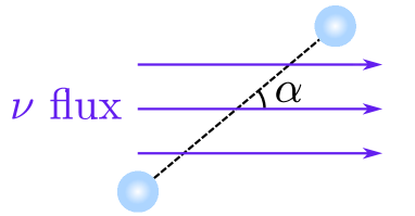
Figure 2: An illustration of neutrino forces between two objects in a directional neutrino flux background.

The anisotropic background leads to an anisotropic scattering amplitude, and hence an anisotropic potential that depends not only on $r$ but also on the angle between $\mathbf{k}_{0}$ and $\mathbf{r}$, denoted by $\alpha$ (cf. Fig. 2). Without loss of generality, we assume $\mathbf{k}_{0}$ is aligned with the $z$-axis and $\mathbf{r}$ lies in the $x$-$z$ plane:

$$\mathbf{k}_{0}=E_{\nu}\left(0,0,1\right),\quad\mathbf{r}=r\left(s_{\alpha},0,c_{\alpha}\right),$$ (46)

where $(c_{\alpha},\ s_{\alpha})\equiv\left(\cos\alpha,\ \sin\alpha\right)$.

Substituting the distribution (45) into Eq. (8), we obtain

$${\cal A}_{{\rm bkg}}\left(\mathbf{q}\right) =2G_{F}^{2}g_{V}^{1}g_{V}^{2}\frac{\Phi_{0}}{E_{\nu}}\left[\frac{2E_{\nu}^{2}+\mathbf{k}_{0}\cdot\mathbf{q}}{\rho^{2}+2\mathbf{k}_{0}\cdot\mathbf{q}}+\frac{2E_{\nu}^{2}-\mathbf{k}_{0}\cdot\mathbf{q}}{\rho^{2}-2\mathbf{k}_{0}\cdot\mathbf{q}}\right]$$

$$=8G_{F}^{2}g_{V}^{1}g_{V}^{2}\Phi_{0}E_{\nu}\frac{1-\xi^{2}}{\rho^{2}-4E_{\nu}^{2}\xi^{2}},$$ (47)

where $\rho\equiv\left|\mathbf{q}\right|$ and

$$\xi\equiv\frac{\mathbf{k}_{0}\cdot\mathbf{q}}{|\mathbf{k}_{0}||\mathbf{q}|}\thinspace.$$ (48)

Note that the typical energy of reactor and solar neutrinos is ${\cal O}$(MeV), so we can safely neglect the neutrino mass in Eq. (8). Thus, the background-induced potential is given by

$$V_{{\rm bkg}}(\mathbf{r})=-\int\frac{d^{3}\mathbf{q}}{\left(2\pi\right)^{3}}e^{i\mathbf{q}\cdot\mathbf{r}}{\cal A}_{{\rm bkg}}(\mathbf{q})=-\frac{g^{1}_{V}g^{2}_{V}}{\pi^{3}}G_{F}^{2}\Phi_{0}E_{\nu}^{2}\times{\cal I}\;,$$ (49)

where ${\cal I}$ is a dimensionless integral. We further define

$$\ell\equiv rE_{\nu}$$ (50)

and note that ${\cal I}$ is depends only on $\ell$ and $\alpha$:

$${\cal I}(\ell,\alpha)\equiv\frac{1}{E_{\nu}}\int d^{3}\mathbf{q}e^{i\mathbf{q}\cdot\mathbf{r}}\frac{1-\xi^{2}}{\rho^{2}-4E_{\nu}^{2}\xi^{2}}\thinspace.$$ (51)

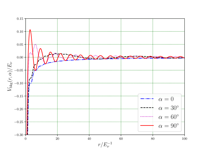
Figure 3: Evolution of the directional background potential with the distance for $\alpha=0$, $30^{\circ}$, $60^{\circ}$ and $90^{\circ}$. Notice that the distance $r$ is in the unit of $E_{\nu}^{-1}$ while the background potential $V_{\rm bkg}(r,\alpha)$ is in the unit of $E_{\nu}$. In addition, an overall dimensionless factor, $G_{F}^{2}g_{V}^{1}g_{V}^{2}\Phi_{0}E_{\nu}$, has been omitted for the background potential.

In Appendix B, we show that, for generic $\alpha$ and $\ell$, the integral can be reduced to

$${\cal I}\left(\ell,\alpha\right)=\frac{\pi^{2}}{2\ell}\left(3+\cos 2\alpha\right)-2\pi\int_{-1}^{1}d\xi\,\xi\left(1-\xi^{2}\right)\int_{0}^{\pi}d\varphi\,\sin\left(2\ell\xi\left|c_{\alpha}\xi+s_{\alpha}\sqrt{1-\xi^{2}}\cos\varphi\right|\right).$$ (52)

For the special cases of $\alpha=0$ and $\alpha=\pi/2$, we find

$${\cal I}\left(\ell,\alpha=0\right) =\frac{\pi^{2}}{\ell}\left[1+\frac{\sin 2\ell}{2\ell}\right]\;,$$ (53)

$${\cal I}\left(\ell,\alpha=\frac{\pi}{2}\right) =\frac{\pi^{2}}{\ell}\left[1-4\ell\int_{0}^{1}d\xi\xi\left(1-\xi^{2}\right)H_{0}\left(2\ell\xi\sqrt{1-\xi^{2}}\right)\right]\;,$$ (54)

where $H_{0}$ is the zeroth-order Struve H function. For generic values of $\alpha$, though we cannot carry out the integration analytically, Eq. (52) can be readily used to compute ${\cal I}\left(\ell,\alpha\right)$ numerically. We have numerically verified that $\int{\cal I}\left(\ell,\alpha\right)dc_{\alpha}$ can reproduce the $r^{-4}$ dependence in Eq. (9), which is expected when Eq. (9) is applied to an isotropic and monochromatic flux. For illustration, in Fig. 3 we show the evolution of the directional background potential $V_{\rm bkg}$ with the distance $r$ for $\alpha=0$, $\pi/6$, $\pi/3$ and $\pi/2$.

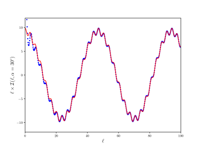
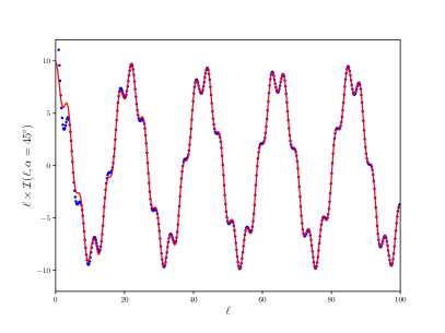
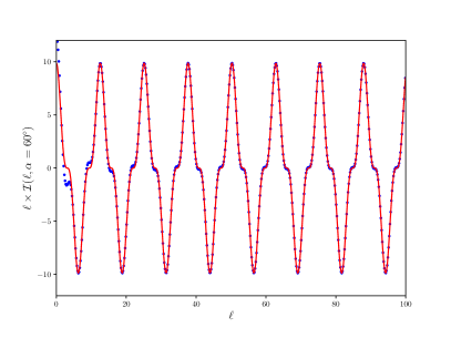
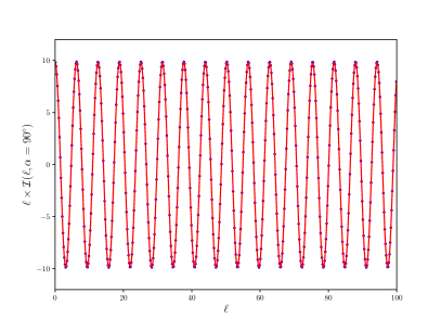
Figure 4: Comparison between the numerical results of $\ell\times{\cal I}(\ell,\alpha)$ computed from Eq. (52) (blue dotted points) and the analytical results computed from Eq. (55) (red solid line) for $\alpha=30^{\circ}$, $\alpha=45^{\circ}$, $\alpha=60^{\circ}$ and $\alpha=90^{\circ}$. They match excellently at large distances (i.e., $r\gg E_{\nu}^{-1}$).

At long distances ($\ell\gg 1$), the numerical evaluation of the double integral in Eq. (52) is computationally expensive. We find that ${\cal I}(\ell,\alpha)$ has a simple analytical expression for $\ell\gg 1$:

$${\cal I}\left(\ell\gg 1,\alpha\right)=\frac{\pi^{2}}{\ell}\cos^{2}\left(\frac{\alpha}{2}\right)\cos\left[\left(1-\cos\alpha\right)\ell\right]+\frac{\pi^{2}}{\ell}\sin^{2}\left(\frac{\alpha}{2}\right)\cos\left[\left(1+\cos\alpha\right)\ell\right]\;.$$ (55)

The analytical formula in Eq. (55) is very efficient to compute the background potential at a long distance. In Fig. 4 we compare the numerical results computed from Eq. (52) with the analytical results from Eq. (55). It can been seen that they match extremely well for $\ell\gg 1$. Recalling $\ell=rE_{\nu}$ the background potential at a long distance is given by

$$V_{\rm bkg}\left(r\gg E_{\nu}^{-1},\alpha\right) = -\frac{g_{V}^{1}g_{V}^{2}}{\pi}G_{F}^{2}\Phi_{0}E_{\nu}\frac{1}{r}\left\{\cos^{2}\left(\frac{\alpha}{2}\right)\cos\left[\left(1-\cos\alpha\right)E_{\nu}r\right]\right.$$ (56)

$$\left.+\sin^{2}\left(\frac{\alpha}{2}\right)\cos\left[\left(1+\cos\alpha\right)E_{\nu}r\right]\right\}\;.$$

We further consider the small $\alpha$ limit ($\alpha\ll 1$ while $E_{\nu}r\alpha^{2}$ can be arbitrarily large) and find

$$V_{\rm bkg}\left(r\gg E_{\nu}^{-1},\alpha\ll 1\right)=-\frac{g_{V}^{1}g_{V}^{2}}{\pi}G_{F}^{2}\times\Phi_{0}E_{\nu}\times\frac{1}{r}\times\cos\left(\frac{\alpha^{2}E_{\nu}r}{2}\right).$$ (57)

A few remarks are in order:

• The first term depends on the couplings of the fermions to the neutrinos.

• The second term is the energy density of the background neutrinos.

• The third term is the leading $r$ dependence. We learn that we have a $1/r$ potential.

• The last term encodes the angular dependency. We discuss it in more detail below.

• To leading order, this effect has no mass dependence. This is because the mass of the neutrino is negligible compared to the energies of the background neutrinos.

We next move to discuss the forces between macroscopic objects. In that case, we need to integrate over the energy of the background neutrinos as well as over the distribution of the masses. This integration can result in a smearing of the force, leading to the oscillatory behavior averaging out as we span the size of the macroscopic objects.

In order to get an effective $1/r$ potential, the smearing should not be very strong. The $\alpha$-suppressed oscillation mode starts to rapidly oscillate when $\alpha^{2}\,\Delta(E_{\nu}\,r)\sim\pi$, where $\Delta(E_{\nu}r)$ is the spread of the energy $E_{\nu}$ and the location of the test masses. So the $1/r$ dependence approximately holds if

$$\alpha^{2}\lesssim\frac{\pi}{\Delta(E_{\nu}\,r)}\thinspace.$$ (58)

4.2 Discussion

The neutrino-force effect is most significant when the background has a direction. There are several significant differences when comparing it to the vacuum case:

1. $r$ dependence. While in vacuum the force scales as $1/r^{5}$, the leading term for a directional background scales as $1/r$. This implies that, at large distances, the background effects always overcome the vacuum contribution. Moreover, it implies that this force scales like gravity and the Coulomb force.

2. Oscillation. The force exhibits oscillatory behavior. The oscillation length depends on the energy of the background neutrinos and the angle spanned by the background’s direction and the direction of the induced force. Only at $\alpha=0$ there is no oscillation.

We provide some intuition for these two effects below. (Some of the discussions below are based on ref. VanTilburg:2024tst ). The point is that, in the presence of background neutrinos, one of the virtual neutrinos in the loop is effectively replaced by a real neutrino, as imposed by the delta function $\delta(k^{2}-m^{2})$ in the background propagator. Then, roughly speaking, the potential is related to the forward scattering amplitude of the real neutrinos between the two objects that are subject to the force. Usually, in the absence of a background, the mass suppression is a result of the “off-shellness” from the momentum transfer $q^{2}$. But in the presence of the high energy directional background, the departure from “off-shellness” is not so straightforward. The situation in vacuum is Lorentz invariant so the departure from $q^{2}$ is simply $m^{2}$. In the presence of the directional background, Lorentz-noninvariant quantities can be present in the propagator, which is what happens in this case.

Thus, in the vacuum case for a one-particle exchange potential, the potential is the Fourier transform of $(\mathbf{q}^{2}+m^{2})^{-1}$, yielding $e^{-mr}/r$. In the background the propagator $\Pi(|\mathbf{q}|^{2})$ is given by (as in Eq. (47)):

$$\Pi(|\mathbf{q}|^{2})\sim{1\over\mathbf{q}^{2}-4E_{\nu}^{2}\cos^{2}\theta_{\mathbf{k}_{0},\mathbf{q}}}={1\over\mathbf{q}^{2}+(2iE_{\nu}\cos\theta_{\mathbf{k}_{0},\mathbf{q}})^{2}},$$ (59)

where $\theta_{\mathbf{k}_{0},\mathbf{q}}$ is the angle between vectors $\mathbf{k}_{0}$ and $\mathbf{q}$ ($\xi\equiv\cos\theta_{\mathbf{k}_{0},\mathbf{q}}$ in Eq. (48)). The propagator has no leading order dependence on $m_{\nu}$ since $E_{\nu}\gg m_{\nu}$. Note that the “off-shellness”, which is real (i.e, $m^{2}$) in the vacuum case, is now imaginary in the presence of the background.

We naively therefore obtain a Fourier transform,

$$V(r)\sim{e^{-2iE_{\nu}rf(\alpha)}\over r}\sim{1\over r}\cos(2E_{\nu}rf(\alpha)),$$ (60)

where $f(\alpha)$ is some function of the angle $\alpha$, which we cannot predict without performing the integral explicitly. This rough form allows us to intuit the features of the potential:

1. The $1/r$ dependence is the geometrical factor for an exchange of a massless intermediate particle. The background neutrinos practically make the potential from a two body exchange into a one body exchange, as evident from Eq. (47). One of the neutrinos is not virtual.

2. The oscillation behavior arises from the fact that the background neutrinos modify the propagator to carry an imaginary “mass term”. This makes the exchanged neutrino “real” as opposed to virtual, giving an oscillatory behavior. Another way this can be understood is as an interference effect between two amplitudes. One amplitude is the incoming background wave and the other one that scatters off one of the two interacting objects. At large $r$, for $\alpha=0$, the interference is pure constructive and the potential behaves as $1/r$, corresponding to $f(0)=0$ in Eq. (60) above. While at $\alpha=\pi/2$, there is destructive interference and oscillatory behavior persists.

5 Experimental sensitivities and detection of neutrino forces

5.1 Current status of the experiments

There have been decades of experimental efforts to search for new long-range forces (also referred to as the fifth force) – see Refs. Wagner:2012ui ; Adelberger:2009zz ; fifth-force for reviews. Searches that typically employ torsion balance devices are closely related to precision tests of gravity, more specifically, to tests of the gravitational inverse-square law (ISL) Hoskins:1985tn ; Lee:2020zjt ; Tan:2020vpf and tests of the weak equivalence principle (WEP) Schlamminger:2007ht ; Smith:1999cr . We summarize the experimental sensitivities in Table 4 and compare them with our theoretical expectations of neutrino forces including background corrections in Fig. 5. The details are explained in what follows.

Experiments testing the WEP look for possible differences between the accelerations of different test bodies in the same gravitational field. For example, the gravitational acceleration on the Earth, $a_{\oplus}\approx 9.8\ {\rm m}/{\rm s}^{2}$, should be universal for all test bodies at the same location, independent of the material of the test body. In the presence of a new long-range force whose couplings to electrons and nucleons are disproportional to their masses, the actual observed acceleration may violate the universality.

exp	$\delta V/V_{{\rm gravity}}$	$\langle r\rangle$	Refs
Washington2007	$3.2\times 10^{-16}$	$\sim 6400$ km	Schlamminger:2007ht
Washington1999	$3.0\times 10^{-9}$	$\sim 0.3$ m	Smith:1999cr
Irvine1985	$0.7\times 10^{-4}$	$2-5$ cm	Hoskins:1985tn
Irvine1985	$2.7\times 10^{-4}$	$5-105$ cm	Hoskins:1985tn
Wuhan2012	$10^{-3}$	$\sim 2$ mm	Yang:2012zzb
Wuhan2020	$3\times 10^{-2}$	$\sim 0.1$ mm	Tan:2020vpf
Washington2020	$\sim 1$	$52$ $\mu$m	Lee:2020zjt
Future levitated optomechanics	$\sim 10^{4}$	1 $\mu$m	Moore:2020awi

Table 4: Sensitivities of long-range force search experiments.

Using Be and Ti as test masses and measuring the difference between their gravitational accelerations, the Washington experiment group reported the following result in 2007 Schlamminger:2007ht :

$$a_{{\rm Be}}-a_{{\rm Ti}}=(0.6\pm 3.1)\times 10^{-15}\ {\rm m}/{\rm s}^{2}\thinspace\ \ ({\rm Earth\ attractor})\thinspace.$$ (61)

Here, the Earth serves as the gravitational attractor. The average distance between particles in the test body and in the attractor in this case is roughly the radius of the Earth, $\langle r\rangle\sim 6400\ {\rm km}$. Dividing the experimental uncertainty in Eq. (61) by $a_{\oplus}\approx 9.8\ {\rm m}/{\rm s}^{2}$, we obtain $\delta V/V_{{\rm gravity}}=3.2\times 10^{-16}$ where $V_{{\rm gravity}}$ is the gravitational potential and $\delta V$ denotes potential variations due to new forces. This experimental setup is referred to as Washington2007 in Table 4.

Instead of making use of the Earth’s gravity, one can also employ laboratory attractors. An earlier experiment conducted by the same group using a 3-ton ²³⁸U attractor and test bodies of Cu and Pb reported Smith:1999cr :

$$a_{{\rm Cu}}-a_{{\rm Pb}}=(1.0\pm 2.8)\times 10^{-15}\ {\rm m}/{\rm s}^{2}\ \ \ \ (\text{3-ton\ ${}^{238}$U attractor})\thinspace.$$ (62)

Note that the uncertainty is close to the one in Eq. (61) but the result should be compared with the gravitational acceleration caused by the ²³⁸U attractor, which is $9.2\times 10^{-7}\ {\rm m}/{\rm s}^{2}$. The ²³⁸U attractor has an annular shape with inner and outer radii of 10.2 cm and 44.6 cm while the torsion balance is located in its center. Hence the average distance between particles in the test body and in the attractor in this case is roughly $\langle r\rangle\sim 0.3\ {\rm m}$. This experimental setup is referred to as Washington1999 in Table 4.

Experiments testing ISL measures the variation of the gravitational attraction between two test bodies when their distance varies. The Irvine experiment conducted in the 1980s was already able to probe ISL over a distance range from 2 cm to 105 cm at the precision of $10^{-4}$Hoskins:1985tn , ruling out a previously claimed deviation of ISL by $(0.37\pm 0.07)\%$ in the 4.5 to 30 cm range long1976experimental . In recent years, the precision of ISL testing experiments in the centimeter to meter range has not been improved significantly. The main progress that has been made so far is the successful measurement of gravitational forces at much smaller distance scales Lee:2020zjt ; Tan:2020vpf . So far, the smallest distance scale at which gravity has been probed in laboratory is $52\ {\rm\mu m}$ Lee:2020zjt . Above this scale, gravitational forces have been measured to certain precision (see results of Wuhan2012 Yang:2012zzb , Wuhan2020 Tan:2020vpf , and Washington2020 Lee:2020zjt in Table 4) and the measurements are fully consistent with ISL.

5.2 Detection of neutrino forces

When applying the above experimental sensitivities to neutrino forces, one should note that $\delta V$ caused by reactor and solar neutrinos are both direction-dependent. For solar neutrinos, the angle $\alpha$ varies with a period of 24 hours due to Earth’s rotation. For reactor neutrinos, the angle $\alpha$ varies in experiments with moving attractors, as is the case of the Washington1999 experiment Smith:1999cr . Since the reactor neutrino flux is only intense within a short distance from a reactor, the Washington2007 experiment does not provide strong probing power to the reactor neutrino force.

In order to compare the deviation of ISL gravitational potential from the background potentials to the experimental sensitivities, we need to compute $V_{\rm bkg}$ between two objects numerically and compare it to the gravity. As a bench mark point, we fix $\alpha=0$.

This assumption is not valid in all of the examples that we study below. All of the current experiments are done between extended objects and the averaging over their shape is important, making the use of the $\alpha=0$ result unjustified. Yet, we do use the $\alpha=0$ as the most optimistic scenario just to get an idea how far the effects are from current sensitivities.

Since in the cases we are considering, the vacuum potential is negligible the neutrino force between two particles in the directional neutrino background is simply given by

$$V_{\nu{\rm-force}}(r)=-\frac{g^{1}_{V}g^{2}_{V}}{\pi}G_{F}^{2}\Phi E_{\nu}\frac{1}{r}\qquad\left(r\gg E_{\nu}^{-1},\leavevmode\nobreak\ \alpha=0\right)\;,$$ (63)

which is proportional to $1/r$, same as the gravitational potential. Notice that the typical energy of reactor and solar neutrino flux is $E_{\nu}\sim{\rm MeV}\sim\left(10^{-11}{\rm cm}\right)^{-1}$, while the average distance between two particles in the test body and in the attractor is larger than ${\rm\mu m}$ (cf. Table 4). Hence, we only need to consider the long-range behavior of the background potential, namely, $r\gg E_{\nu}^{-1}$. We use Eq. (63) below to compute the background potentials.

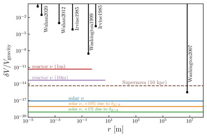
Figure 5: Neutrino forces in comparison with experimental sensitivities. Here all neutrino sources are assumed to be ideally point-like and the angular spread is assumed to be sufficiently small to meet Eq. (58). In reality, a sizable angular spread needs to be taken into account thus the above should be considered as an upper bound of the effect.

In Fig. 5, we plot the reactor neutrino force curves calculated from Eq. (63) using the standard reactor neutrino flux at 1 meter and 10 meters from the reactor core. For a reactor with 2.9 GW thermal power, the neutrino flux is $\Phi=5\times 10^{13}\ {\rm cm}^{-2}{\rm s}^{-1}$ at 10 meters away Kopeikin:2012zz . We take $E_{\nu}$ in Eq. (63) to be 2 MeV when computing the background potential from reactor neutrinos. The curves stop at $r=0.5$ m and $r=5$ m because experiments with much larger $r$ (such as Washington2007) are impossible to have test bodies and attractors all fitted in the limited space within 1 or 10 meters from the reactor.

For solar neutrinos, this is not a concern. So far, all experiments have $r$ much smaller than the distance to the Sun. However, one should note that the angle $\alpha$ varies with a period of 24 hours while a large number of noises are also 24-hour periodic. Hence the $\alpha$ dependence could be easily submerged in such noises. Nevertheless, we plot the solar neutrino line in Fig. 5 assuming that it could be resolved among various noises in future experiments.

The solar neutrino line in Fig. 5 is calculated from Eq. (63) by considering $pp$ neutrinos with the flux $\Phi=5.99\times 10^{10}{\rm cm}^{-2}{\rm s}^{-1}$ and the highest energy $E_{\rm max}=0.42{\rm\,MeV}$ Vinyoles:2016djt . In the computation we take $E_{\nu}=0.3{\rm\,MeV}$ since the $pp$ neutrino spectrum is not monochromatic. We have also calculated the background potential of the ⁷Be solar neutrinos whose flux is $\Phi=4.84\times 10^{9}{\rm\,cm}^{-2}{\rm s}^{-1}$ with two monochromatic energies being $E_{\nu}=0.862{\rm\,MeV}$ and $E_{\nu}=0.384\,{\rm MeV}$ Vinyoles:2016djt . But the result is the same order of magnitude as that of $pp$ neutrinos.

It might be more feasible to make use of the material dependence feature of neutrino forces. Since the effective neutrino-proton vector coupling is suppressed by a factor of $1-4\sin^{2}\theta_{W}\approx 0.05$ with respect to the effective neutrino-neutron vector coupling, we can assume that neutrino forces mainly depend on the neutron number $N=A-Z$ ($A$: atomic mass number, $Z$: proton number) of the material used in test bodies. The contribution of electrons is more complicated since the charged-current interaction may or may not contribute (if not, the $1-4\sin^{2}\theta_{W}$ suppression also applies to electrons), depending on the neutrino flavor. For simplicity, here we neglect the electron contribution (see Appendix D for a more strict treatment). Therefore, for neutrino forces on different materials, the difference is roughly

$$\frac{\delta V_{\nu{\rm-force}}}{V_{\nu{\rm-force}}}\sim\delta_{Z/A},\ \delta_{Z/A}=\begin{cases}1.6\%&\text{for Be vs Ti }\\ 4.9\%&\text{for Cu vs Pb }\\ 8.2\%&\text{for Al vs Pt }\end{cases}.$$ (64)

Here $Z/A$ is approximately $1/2$ for most nuclei, and $\ \delta_{Z/A}$ denotes its variation for different materials. Taking Be vs Ti for example, since Ti (Be) has 22 (4) protons and 26 (5) neutrons, the difference is $22/48-4/9=1.4\%$. More accurate calculations using $A=47.87$ ($9.012$) gives $1.6\%$. In principle, $\delta_{Z/A}$ could be enhanced to as large as $50\%$ if Hydrogen ($Z=A=1$) is used in combination with other $Z/A\approx 1/2$ material, though technically it is difficult to make test bodies of Hydrogen. In Fig. 5, below the solar neutrino line, we plot two lines by multiplying it with $\delta_{Z/A}=10\%$ and $1\%$. If the direction-dependent signal of $V_{\nu{\rm-force}}$ are submerged in various 24-hour noises, the material dependence of $V_{\nu{\rm-force}}$, which is a factor of $\delta_{Z/A}$ weaker but more robust against noises, could be exploited to probe neutrino forces.

In addition to the aforementioned dependence on directions and materials, the difference between reactor-on and -off measurements could also be used to probe neutrino forces.

For supernova neutrinos, we plot a dashed line in Fig. 5 to present the magnitude. We assume that the supernova neutrino flux is $10^{12}\ {\rm cm}^{-2}{\rm s}^{-1}$, corresponding to a 10 kpc core-collapse supernova neutrino burst Kachelriess:2004ds . The neutrino mean energy is about $10$ MeV. Here we use a dashed line to remind the readers that such a neutrino burst lasts only for a short period of a few seconds, which might be too short for torsion balance experiments to reach the desired sensitivity (e.g. the torsional oscillation period of Washington 2007 is 798 s Schlamminger:2007ht ). A dedicated analysis on such experiments taking the short duration into consideration might lead to a much weaker sensitivity, but this is beyond the scope of our work.

At last, we give some brief remarks on the background effects from atmospheric and accelerator neutrinos. The flux of atmospheric neutrinos is much smaller than those of the reactor and solar neutrinos Raffelt2020 . As a result, the corresponding background potential is weaker than that of reactor neutrinos by 12 orders of magnitude. In addition, the flux from long-baseline accelerator neutrino experiments like DUNE DUNE:2020lwj is also weaker than that of reactor neutrinos. The accelerator neutrino background potential at the near-detector location of DUNE is about 7 orders of magnitude smaller than that of reactor neutrinos. Therefore, the background potentials from both atmospheric and accelerator neutrinos are out of the reach with current experimental sensitivities.

6 Conclusions

In this paper, we computed the background corrections to neutrino forces in a thermal or non-thermal neutrino background. We found that the presence of the background can significantly increase the strength of neutrino forces.

For the isotropic C$\nu$B in Eq. (13), we have derived general formulae of the background potential for both Dirac [Eq. (26)] and Majorana [Eq. (41)] neutrinos that are valid for arbitrary neutrino masses and distances. The main feature of the potential in the presence of the C$\nu$B is that, at large distances ($r\gg m_{\nu}^{-1}$), it is not exponentially suppressed, as opposed to the potential in vacuum. Therefore, when the distance between two particles exceeds the inverse mass of neutrinos, the neutrino force between them is dominated by the background contribution. However, since the number density of the cosmic neutrinos is very small today, the thermal effects of the C$\nu$B on the neutrino force are still far from the available experimental sensitivities.

We then computed the neutrino force in a directional background. We parametrized the non-thermal and anisotropic background as monochromatic distribution function with a specific direction, $\alpha$. The general direction-dependent background potential is given by Eqs. (49) and (52). At $r\gg E_{\nu}^{-1}$ with $E_{\nu}$ being the typical energy of the neutrino flux, the background potential in the small $\alpha$ limit is proportional to $1/r$, which falls much slower than the $1/r^{5}$ potential in vacuum and in isotropic backgrounds. In particular, there is a potential significant enhancement of the vacuum force in the presence of directional energetic dense neutrino backgrounds.

We then turned to discuss the possibility of probing the neutrino force using torsion balance experiments that aim to precisely test the gravitational inverse-square law and the weak equivalence principle. Assuming the small $\alpha$ limit, the comparison of the neutrino force in reactor and solar neutrino backgrounds with experimental sensitivities is summarized in Fig. 5. The figure shows that, if Eq. (58) could be satisfied, the current experiments would be 2 or 3 orders of magnitude far from detecting neutrino forces in the reactor or solar neutrino background. With current technology, however, the condition in Eq. (58) is not satisfied and the energy and angular spread smear out the leading $1/r$ potential. While it is not clear to us how complicated and practical it is to design an experiment that can exploit the enhancement we discuss, the point to emphasize is that strong enhancement is present.

We conclude that the neutrino force in the solar or reactor neutrino background is much more experimentally accessible than the one in vacuum. Dedicated experimental efforts are called for to check if these enhancement factors can be exploit in order to detect the elusive neutrino force.

Note added. After we updated our paper on arXiv to Version 2, Ref. Blas:2022ovz appeared on arXiv. The authors of that preprint commented that the finite size of the wave packets would destroy the leading $1/r$ potential in directional neutrino backgrounds that we found. However, the content of Blas:2022ovz was referring to Version 1 of our paper, while in Version 2 we have already addressed the smearing effect. To address the effect of the smearing, Ref. Blas:2022ovz took a different approach than ours. They included the energy spread in the wave packets first and then took a monochromatic directional flux and fixed $\alpha=0$, while we consider the smearing effect by varying $E_{\nu}$ and $\alpha$ of the flux. While the details of our analyses are not identical, the results of the current version of our work are in agreement with the results of Ref. Blas:2022ovz . Yet, our conclusions have a different tone. While we emphasize the fact that there is indeed a strong enhancement when Eq. (58) is satisfied, Ref. Blas:2022ovz is worried about the feasibility of designing experiments that can use it.

Appendix A The background effect on fermion propagators

The neutrino propagator in a background with finite neutrino number density in Eq. (4) can be found in various references including books and reviews on finite temperature field theory Landsman:1986uw ; Notzold:1987ik ; Quiros:1999jp ; Kapusta:2006pm ; Laine:2016hma . In this appendix, we provide a simple and pedagogical re-derivation of the formula without using finite temperature field theory, aiming at providing a physical interpretation of the background effect.

Let us start with the propagator of a generic fermion in vacuum, which is defined as

$$S_{F}(x-y)\equiv\langle 0|T\psi(x)\overline{\psi(y)}|0\rangle\thinspace,$$ (65)

where $T$ indicates that it is a time-ordered product. Using

$$\psi=\int\frac{d^{3}\mathbf{p}}{(2\pi)^{3}}\frac{1}{\sqrt{2E_{\mathbf{p}}}}\sum_{s}\left[a_{\mathbf{p}}^{s}u^{s}(p)e^{-ip\cdot x}+b_{\mathbf{p}}^{s\dagger}v^{s}(p)e^{ip\cdot x}\right],$$ (66)

where we follow the standard notation of Ref. Peskin , and assuming $x^{0}>y^{0}$ so that $T$ can be removed, we obtain

$$S_{F} \propto\int\frac{d^{3}\mathbf{p}}{(2\pi)^{3}}\int\frac{d^{3}\mathbf{k}}{(2\pi)^{3}}\frac{1}{\sqrt{2E_{\mathbf{p}}}}\frac{1}{\sqrt{2E_{\mathbf{k}}}}e^{-ip\cdot x+ik\cdot y}\langle 0|a_{\mathbf{p}}a_{\mathbf{k}}^{\dagger}|0\rangle+\cdots,$$ (67)

where for brevity we have neglected $u^{s}$, $v^{s}$, and the script $s$ (they only affect the structure of Dirac spinors). The “$\cdots$” denote terms proportional to $\langle 0|a_{\mathbf{p}}b_{\mathbf{k}}|0\rangle,$ $\langle 0|b_{\mathbf{p}}^{\dagger}a_{\mathbf{k}}^{\dagger}|0\rangle$, or $\langle 0|b_{\mathbf{p}}^{\dagger}b_{\mathbf{k}}|0\rangle$, all being zero. Since $\langle 0|a_{\mathbf{p}}a_{\mathbf{k}}^{\dagger}|0\rangle=(2\pi)^{3}\delta^{3}(\mathbf{p}-\mathbf{k})$, Eq. (67) gives

$$S_{F}\propto \int\frac{d^{3}\mathbf{p}}{(2\pi)^{3}}\frac{1}{2E_{\mathbf{p}}}e^{-ip\cdot(x-y)}=\int\frac{d^{4}p}{(2\pi)^{4}}\frac{i}{p^{2}-m^{2}+i\epsilon}e^{-ip\cdot(x-y)}\thinspace.$$ (68)

The last step is simply the reverse process of computing the contour integral of $p^{0}$, with the underlying assumption that $x^{0}>y^{0}$. For $x^{0}<y^{0}$, the time ordering guarantees the same result.

Now we shall replace $|0\rangle$ with a background state. Let us first consider a single-particle state which contains a particle with an almost certain position and an almost certain momentum. The two cannot be simultaneously fixed at exact values due to the uncertainty principle, but one can nevertheless introduce a wave package function $w(\mathbf{p})$ so that both $w(\mathbf{p})$ and its Fourier transform $\int w(\mathbf{p})e^{i\mathbf{p}\cdot\mathbf{x}}d^{3}\mathbf{x}$ are limited in a small region of their respective space—for further elucidation, see e.g. Appendix A of Ref. Smirnov:2022sfo . The single particle state is then defined as

$$|w\rangle=\int\frac{d^{3}\mathbf{p}}{(2\pi)^{3}}w(\mathbf{p})a_{\mathbf{p}}^{\dagger}|0\rangle\thinspace,\ \langle w|w\rangle=\int\frac{d^{3}\mathbf{p}}{(2\pi)^{3}}|w(\mathbf{p})|^{2}\equiv 1\thinspace,$$ (69)

where the last step is defined as the normalization condition of $w(\mathbf{p})$.

Replacing $|0\rangle\to|w\rangle$ in Eq. (67), we obtain

$$S_{F}\propto\int_{\mathbf{p}\mathbf{k}}\langle w|a_{\mathbf{p}}a_{\mathbf{k}}^{\dagger}|w\rangle=\int_{\mathbf{p}\mathbf{k}}\left\langle w\left|\left((2\pi)^{3}\delta^{3}(\mathbf{p}-\mathbf{k})-a_{\mathbf{k}}^{\dagger}a_{\mathbf{p}}\right)\right|w\right\rangle\thinspace,$$ (70)

where $\int_{\mathbf{p}\mathbf{k}}$ standards for $\int\frac{d^{3}\mathbf{p}}{(2\pi)^{3}}\int\frac{d^{3}\mathbf{k}}{(2\pi)^{3}}\frac{1}{\sqrt{2E_{\mathbf{p}}}}\frac{1}{\sqrt{2E_{\mathbf{k}}}}e^{-ip\cdot x+ik\cdot y}$. Since $\langle w|w\rangle=1$, the first term leads to the same result as the vacuum case and the second term represents the background effect. We denote the contribution of the latter by $S_{F}^{{\rm bkg}}$:

$$S_{F}^{{\rm bkg}}\propto-\int_{\mathbf{p}\mathbf{k}}\langle w|a_{\mathbf{k}}^{\dagger}a_{\mathbf{p}}|w\rangle=-\int_{\mathbf{p}\mathbf{k}}w^{*}(\mathbf{k})w(\mathbf{p})\thinspace,$$ (71)

where we have used $a_{\mathbf{p}}|w\rangle=w(\mathbf{p})|0\rangle$. Note that $w(\mathbf{p})$ has been defined in such a way that the particle’s position and momentum are nearly fixed at certain values (say $\mathbf{x}_{0}$ and $\mathbf{p}_{0}$). One can perform spatial translation of the wave package $w(\mathbf{p})\to w_{\Delta\mathbf{x}}(\mathbf{p})\equiv e^{i\mathbf{p}\cdot\Delta\mathbf{x}}w(\mathbf{p})$ so that its position is changed to $\mathbf{x}_{0}+\Delta\mathbf{x}$ while the momentum is unchanged. Now, if we randomly choose $\Delta\mathbf{x}$ with a uniform probability distribution in a large volume $V$ (much larger than the distribution of each wave package), the position of the particle would be evenly smeared in $V$. For $w^{*}(\mathbf{k})w(\mathbf{p})$ in Eq. (71), the smearing leads to

$$w^{*}(\mathbf{k})w(\mathbf{p})\xrightarrow{\text{smearing}} \frac{1}{V}\int w_{\Delta\mathbf{x}}^{*}(\mathbf{k})w_{\Delta\mathbf{x}}(\mathbf{p})d^{3}\Delta\mathbf{x}$$

$$=\frac{1}{V}\int w^{*}(\mathbf{k})w(\mathbf{p})e^{i(\mathbf{p}-\mathbf{k})\cdot\Delta\mathbf{x}}d^{3}\Delta\mathbf{x}$$

$$=\frac{(2\pi)^{3}\delta^{3}(\mathbf{p}-\mathbf{k})}{V}|w(\mathbf{p})|^{2}$$

$$=(2\pi)^{3}\delta^{3}(\mathbf{p}-\mathbf{k})n_{+}(\mathbf{p})\thinspace,$$ (72)

where in the last step we have identified $|w(\mathbf{p})|^{2}/V$ as $n_{+}(\mathbf{p})$ because $\int\frac{d^{3}\mathbf{p}}{(2\pi)^{3}}|w(\mathbf{p})|^{2}=1$ and the number density after smearing is $\int\frac{d^{3}\mathbf{p}}{(2\pi)^{3}}n_{+}(\mathbf{p})=1/V$.

Substituting Eq. (72) into Eq. (71), we obtain

$$-\int_{\mathbf{p}\mathbf{k}}w^{*}(\mathbf{k})w(\mathbf{p})\xrightarrow{\text{smearing}} -\int\frac{d^{3}\mathbf{p}}{(2\pi)^{3}}\frac{e^{-ip\cdot(x-y)}}{2E_{\mathbf{p}}}n_{+}(\mathbf{p})$$

$$=-\int\frac{d^{4}p}{(2\pi)^{4}}e^{-ip\cdot(x-y)}(2\pi)\delta\left(p^{2}-m^{2}\right)\Theta\left(p^{0}\right)n_{+}(\mathbf{p})\thinspace.$$ (73)

Combining Eq. (73) with the vacuum part in Eq. (68), we obtain

$$S_{F}\propto\int\frac{d^{4}p}{(2\pi)^{4}}e^{-ip\cdot(x-y)}\left\{\frac{i}{p^{2}-m^{2}+i\epsilon}-(2\pi)\delta\left(p^{2}-m^{2}\right)\Theta\left(p^{0}\right)n_{+}(\mathbf{p})\right\}\thinspace.$$ (74)

For an anti-particle background, the above calculation is similar except that some minus signs are flipped. In the presence of both particles and anti-particles in the background, we obtain

$$S_{F}(p) =\left(\not{p}+m\right)\left\{\frac{i}{p^{2}-m^{2}+i\epsilon}-(2\pi)\delta\left(p^{2}-m^{2}\right)\Theta\left(p^{0}\right)\left[n_{+}(\mathbf{p})-n_{-}(\mathbf{p})\right]\right\}$$

$$=\left(\not{p}+m\right)\left\{\frac{i}{p^{2}-m^{2}+i\epsilon}-(2\pi)\delta\left(p^{2}-m^{2}\right)\left[\Theta\left(p^{0}\right)n_{+}(\mathbf{p})+\Theta\left(-p^{0}\right)n_{-}(\mathbf{p})\right]\right\},$$

where $S_{F}(p)$ is the propagator in the momentum space [i.e. the Fourier transform of $S_{F}(x-y)$], the prefactor $\left(\not{p}+m\right)$ can be inferred from the vacuum propagator. The result is the same as the fermion propagator derived in finite temperature field theory.

From the above calculation, one can see that the background effect comes from the second term in Eq. (70), proportional to $\langle w|a_{\mathbf{k}}^{\dagger}a_{\mathbf{p}}|w\rangle$. Recall that the annihilation operator $a_{\mathbf{p}}$ acting on $|w\rangle$ can be interpreted as reducing one particle in the background. Hence $\langle w|a_{\mathbf{k}}^{\dagger}a_{\mathbf{p}}|w\rangle$ corresponds to first absorbing a particle of momentum $\mathbf{p}$ from the background ($a_{\mathbf{p}}|w\rangle=w(\mathbf{p})|0\rangle$), and returning a particle of momentum $\mathbf{k}$ back to the background. Smearing the single particle state in Eq. (72) leads to $\delta^{3}(\mathbf{p}-\mathbf{k})$, which guarantees that the particle being returned has the same momentum as the one being absorbed.

Intuitively, the modified propagator in Eq. (4) can be understood as the vacuum expectation value of two fermion fields with the vacuum state $|0\rangle$ replaced by the modified background state $|w\rangle$, which is the vacuum equipped with some on-shell background fermions. Then the Wick contraction can be carried out not only between the two internal fermion fields (leading to the vacuum propagator), but also among the internal fields and the background fermions (leading to the modified term). Therefore, the modified term is naturally proportional to the number density of background fermions, with the factor $2\pi\delta(p^{2}-m^{2})\Theta(p^{0})$ coming from cutting the propagator to put it on-shell (optical theorem). Notice that the above arguments should be valid in any background and do not require the distribution to be thermal.

Appendix B Integrals

In this appendix, we present the details about some integrals in calculating neutrino forces in the neutrino backgrounds.

B.1 Derivation of the general background potential $V_{\rm bkg}(r)$ in Eq. (9)

We first show how to obtain the general expression of the background potential with an arbitrary distribution function.

As has been stated above, when both neutrino propagators in Eq. (6) take the first part, it corresponds to the vacuum potential $V_{0}(r)$, which is independent of the background distribution functions. When both propagators take the second part, the result always vanishes because of the existence of two delta functions. Therefore, the background contribution comes from the cross terms, i.e., $S_{\nu}(k)$ takes the first (second) part and $S_{\nu}(k+q)$ takes the second (first) part:

$${\cal A}_{{\rm bkg}}(q) = -\pi G_{F}^{2}g^{1}_{V}g^{2}_{V}\int\frac{d^{4}k}{\left(2\pi\right)^{4}}\delta\left(k^{2}-m_{\nu}^{2}\right)\left[\Theta\left(k^{0}\right)n_{+}\left(\mathbf{k}\right)+\Theta\left(-k^{0}\right)n_{-}\left(\mathbf{k}\right)\right]$$ (75)

$$\times\left\{\frac{{\rm Tr}\left[\gamma^{0}\left(1-\gamma_{5}\right)\left(\not{k}+m_{\nu}\right)\gamma^{0}\left(1-\gamma_{5}\right)\left(\not{k}+\not{q}+m_{\nu}\right)\right]}{\left(k+q\right)^{2}-m_{\nu}^{2}}\right.$$

$$\left.+\frac{{\rm Tr}\left[\gamma^{0}\left(1-\gamma_{5}\right)\left(\not{k}-\not{q}+m_{\nu}\right)\gamma^{0}\left(1-\gamma_{5}\right)\left(\not{k}+m_{\nu}\right)\right]}{\left(k-q\right)^{2}-m_{\nu}^{2}}\right\}\,,\;$$

$$= -8\pi G_{F}^{2}g^{1}_{V}g^{2}_{V}\int\frac{d^{4}k}{\left(2\pi\right)^{4}}\delta\left(k^{2}-m_{\nu}^{2}\right)\left[\Theta\left(k^{0}\right)n_{+}\left(\mathbf{k}\right)+\Theta\left(-k^{0}\right)n_{-}\left(\mathbf{k}\right)\right]$$

$$\times\left[\frac{2k^{0}\left(k^{0}+q^{0}\right)-\left(k\cdot q+k^{2}\right)}{\left(k+q\right)^{2}-m_{\nu}^{2}}+\frac{2k^{0}\left(k^{0}-q^{0}\right)+\left(k\cdot q-k^{2}\right)}{\left(k-q\right)^{2}-m_{\nu}^{2}}\right]\;.$$

Taking advantage of the identity

$$\delta\left(k^{2}-m_{\nu}^{2}\right)=\delta\left(\left(k^{0}\right)^{2}-E_{k}^{2}\right)=\frac{1}{2E_{k}}\left[\delta\left(k^{0}-E_{k}\right)+\delta\left(k^{0}+E_{k}\right)\right]\;,$$

one can first integrate $k^{0}$ in Eq. (75). In addition, the NR approximation requires $q\simeq\left(0,\mathbf{q}\right)$. Thus the integral in Eq. (75) can be reduced to Eq. (8)

$${\cal A}_{{\rm bkg}}(\mathbf{q})=4G_{F}^{2}g^{1}_{V}g^{2}_{V}\int\frac{d^{3}\mathbf{k}}{\left(2\pi\right)^{3}}\frac{n_{+}\left(\mathbf{k}\right)+n_{-}\left(\mathbf{k}\right)}{2E_{k}}\left[\frac{2\left|\mathbf{k}\right|^{2}+m_{\nu}^{2}+\mathbf{k}\cdot\mathbf{q}}{2\mathbf{k}\cdot\mathbf{q}+\left|\mathbf{q}\right|^{2}}+\left(\mathbf{k}\to-\mathbf{k}\right)\right].$$ (76)

Furthermore, for an isotropic distribution, $n_{\pm}\left(\mathbf{k}\right)=n_{\pm}\left(\kappa\right)$ with $\kappa\equiv\left|\mathbf{k}\right|$, one can first integrate out the angular part in Eq. (76) and obtains

$${\cal A}_{{\rm bkg}}(\rho)=\frac{G_{F}^{2}g^{1}_{V}g^{2}_{V}}{\pi^{2}}\int_{0}^{\infty}d\kappa\frac{\kappa^{2}}{\sqrt{\kappa^{2}+m_{\nu}^{2}}}\left[n_{+}\left(\kappa\right)+n_{-}\left(\kappa\right)\right]\int_{-1}^{1}d\xi\frac{m_{\nu}^{2}+2\kappa^{2}\left(1-\xi^{2}\right)}{\rho^{2}-4\kappa^{2}\xi^{2}}\;,$$ (77)

where we have defined $\rho\equiv\left|\vec{q}\right|$ and $\xi\equiv\cos\theta$ with $\theta$ being the angel between $\mathbf{k}$ and $\mathbf{q}$. Then the background potential is given by

$$V_{{\rm bkg}}(r) = -\int\frac{d^{3}\mathbf{q}}{\left(2\pi\right)^{3}}e^{i\mathbf{q}\cdot\mathbf{r}}{\cal A}_{\rm bkg}(\rho)=-\frac{1}{2\pi^{2}r}\int_{0}^{\infty}d\rho\rho\sin\left(\rho r\right){\cal A}_{\rm bkg}(\rho)$$ (78)

$$= -\frac{G_{F}^{2}g^{1}_{V}g^{2}_{V}}{2\pi^{4}r}\int_{0}^{\infty}d\kappa\frac{\kappa^{2}}{\sqrt{\kappa^{2}+m_{\nu}^{2}}}\left[n_{+}\left(\kappa\right)+n_{-}\left(\kappa\right)\right]\int_{-1}^{1}d\xi\left[m_{\nu}^{2}+2\kappa^{2}\left(1-\xi^{2}\right)\right]\int_{0}^{\infty}d\rho\frac{\rho\sin\left(\rho r\right)}{\rho^{2}-4\kappa^{2}\xi^{2}}$$

$$= -\frac{G_{F}^{2}g^{1}_{V}g^{2}_{V}}{4\pi^{3}r}\int_{0}^{\infty}d\kappa\frac{\kappa^{2}}{\sqrt{\kappa^{2}+m_{\nu}^{2}}}\left[n_{+}\left(\kappa\right)+n_{-}\left(\kappa\right)\right]\int_{-1}^{1}d\xi\left[m_{\nu}^{2}+2\kappa^{2}\left(1-\xi^{2}\right)\right]\cos\left(2\kappa r\xi\right)$$

$$= -\frac{G_{F}^{2}g^{1}_{V}g^{2}_{V}}{4\pi^{3}r^{4}}\int_{0}^{\infty}\frac{d\kappa\kappa}{\sqrt{\kappa^{2}+m_{\nu}^{2}}}\left[n_{+}\left(\kappa\right)+n_{-}\left(\kappa\right)\right]\left[\left(1+m_{\nu}^{2}r^{2}\right)\sin\left(2\kappa r\right)-2\kappa r\cos\left(2\kappa r\right)\right]\;,$$

which is just Eq. (9).

B.2 Calculation of the integral ${\cal I}(\ell,\alpha)$ in Eq. (51)

Here, we calculate the integral ${\cal I}(\ell,\alpha)$ appearing in the reactor neutrino background. Without loss of generality, we can assume

$$\mathbf{k}_{0}=E_{\nu}\left(0,0,1\right)\;,\quad\mathbf{r}=r\left(s_{\alpha},0,c_{\alpha}\right)\;,\quad\mathbf{q}=\rho\left(s_{\theta}c_{\varphi},s_{\theta}s_{\varphi},c_{\theta}\right)\;,$$ (79)

where $(c_{x},s_{x})\equiv\left(\cos x,\sin x\right)$ have been defined. With the above coordinates, we have

$$\mathbf{q}\cdot\mathbf{r}=\rho r\left(s_{\alpha}s_{\theta}c_{\varphi}+c_{\alpha}c_{\theta}\right)\;,\quad\xi\equiv\frac{\mathbf{k_{0}}\cdot\mathbf{q}}{\left|\mathbf{k_{0}}\right|\left|\mathbf{q}\right|}=c_{\theta}\;,\quad\int d^{3}\mathbf{q}=\int_{0}^{\infty}\rho^{2}d\rho\int_{-1}^{1}d\xi\int_{0}^{2\pi}d\varphi\;.$$ (80)

The integral in Eq. (51) turns out to be

$${\cal I} \equiv \frac{1}{E_{\nu}}\int d^{3}\mathbf{q}e^{i\mathbf{q}\cdot\mathbf{r}}\frac{1-\xi^{2}}{\rho^{2}-4E_{\nu}^{2}\xi^{2}}=\frac{1}{E_{\nu}}\int_{0}^{2\pi}d\varphi\int_{-1}^{1}d\xi\int_{0}^{\infty}d\rho e^{i\rho r(s_{\alpha}s_{\theta}c_{\varphi}+c_{\alpha}c_{\theta})}\frac{\rho^{2}\left(1-\xi^{2}\right)}{\rho^{2}-4E_{\nu}^{2}\xi^{2}}$$

$$= \frac{1}{E_{\nu}}\left(\int_{0}^{2\pi}d\varphi\int_{0}^{1}d\xi\int_{0}^{\infty}d\rho+\int_{0}^{2\pi}d\varphi\int_{-1}^{0}d\xi\int_{0}^{\infty}d\rho\right)e^{i\rho r(s_{\alpha}s_{\theta}c_{\varphi}+c_{\alpha}c_{\theta})}\frac{\rho^{2}\left(1-\xi^{2}\right)}{\rho^{2}-4E_{\nu}^{2}\xi^{2}}\;.$$

In the second term in the bracket of Eq. (B.2), changing the variables as $\rho\to-\rho$ and $\xi\to-\xi$ one obtains

$${\cal I} = \frac{1}{E_{\nu}}\int_{0}^{2\pi}d\varphi\int_{0}^{1}d\xi\left[\int_{0}^{\infty}d\rho e^{i\rho r(s_{\alpha}s_{\theta}c_{\varphi}+c_{\alpha}c_{\theta})}+\int_{-\infty}^{0}d\rho e^{i\rho r(-s_{\alpha}s_{\theta}c_{\varphi}+c_{\alpha}c_{\theta})}\right]\frac{\rho^{2}\left(1-\xi^{2}\right)}{\rho^{2}-4E_{\nu}^{2}\xi^{2}}$$

$$= \frac{1}{E_{\nu}}\int_{0}^{\pi}d\varphi\int_{0}^{1}d\xi\left[\int_{0}^{\infty}d\rho e^{i\rho r(s_{\alpha}s_{\theta}c_{\varphi}+c_{\alpha}c_{\theta})}+\int_{-\infty}^{0}d\rho e^{i\rho r(-s_{\alpha}s_{\theta}c_{\varphi}+c_{\alpha}c_{\theta})}\right]\frac{\rho^{2}\left(1-\xi^{2}\right)}{\rho^{2}-4E_{\nu}^{2}\xi^{2}}$$

$$+ \frac{1}{E_{\nu}}\int_{\pi}^{2\pi}d\varphi\int_{0}^{1}d\xi\left[\int_{0}^{\infty}d\rho e^{i\rho r(s_{\alpha}s_{\theta}c_{\varphi}+c_{\alpha}c_{\theta})}+\int_{-\infty}^{0}d\rho e^{i\rho r(-s_{\alpha}s_{\theta}c_{\varphi}+c_{\alpha}c_{\theta})}\right]\frac{\rho^{2}\left(1-\xi^{2}\right)}{\rho^{2}-4E_{\nu}^{2}\xi^{2}}\;.$$

In the last line of Eq. (B.2) changing the variable $\varphi\to\varphi-\pi$ one obtains

$${\cal I} = \frac{1}{E_{\nu}}\int_{0}^{\pi}d\varphi\int_{0}^{1}d\xi\left[\int_{0}^{\infty}d\rho e^{i\rho r(s_{\alpha}s_{\theta}c_{\varphi}+c_{\alpha}c_{\theta})}+\int_{-\infty}^{0}d\rho e^{i\rho r(-s_{\alpha}s_{\theta}c_{\varphi}+c_{\alpha}c_{\theta})}\right]\frac{\rho^{2}\left(1-\xi^{2}\right)}{\rho^{2}-4E_{\nu}^{2}\xi^{2}}$$

$$+ \frac{1}{E_{\nu}}\int_{0}^{\pi}d\varphi\int_{0}^{1}d\xi\left[\int_{0}^{\infty}d\rho e^{i\rho r(-s_{\alpha}s_{\theta}c_{\varphi}+c_{\alpha}c_{\theta})}+\int_{-\infty}^{0}d\rho e^{i\rho r(s_{\alpha}s_{\theta}c_{\varphi}+c_{\alpha}c_{\theta})}\right]\frac{\rho^{2}\left(1-\xi^{2}\right)}{\rho^{2}-4E_{\nu}^{2}\xi^{2}}$$

$$= \frac{1}{E_{\nu}}\int_{0}^{\pi}d\varphi\int_{0}^{1}d\xi\left(1-\xi^{2}\right)\int_{-\infty}^{\infty}d\rho\left[e^{i\rho r(s_{\alpha}s_{\theta}c_{\varphi}+c_{\alpha}c_{\theta})}+e^{i\rho r(-s_{\alpha}s_{\theta}c_{\varphi}+c_{\alpha}c_{\theta})}\right]\frac{\rho^{2}}{\rho^{2}-4E_{\nu}^{2}\xi^{2}}\;.$$

What we have done is to change the integral to the standard form of one-dimensional Fourier transform. Then one can use the following Fourier transform:

$$\int_{-\infty}^{\infty}d\rho e^{i\rho x}\frac{\rho^{2}}{\rho^{2}-4E_{\nu}^{2}\xi^{2}}=2\pi\left[\delta(x)-{\rm sgn}(x)E_{\nu}\xi\sin\left(2E_{\nu}\xi x\right)\right]\;,$$ (84)

from which one obtains

$${\cal I} = \frac{2\pi}{E_{\nu}}\int_{0}^{\pi}d\varphi\int_{0}^{1}d\xi\left(1-\xi^{2}\right)\left[\delta\left(x_{+}\right)-{\rm sgn}\left(x_{+}\right)E_{\nu}\xi\sin\left(2E_{\nu}\xi x_{+}\right)\right.$$ (85)

$$\left.+\delta\left(x_{-}\right)-{\rm sgn}\left(x_{-}\right)E_{\nu}\xi\sin\left(2E_{\nu}\xi x_{-}\right)\right]$$

$$= \frac{2\pi}{E_{\nu}}\int_{-1}^{1}d\xi\left(1-\xi^{2}\right)\int_{0}^{\pi}d\varphi\left[\delta\left(x_{+}\right)-{\rm sgn}\left(x_{+}\right)E_{\nu}\xi\sin\left(2E_{\nu}\xi x_{+}\right)\right]$$

where $x_{\pm}\equiv r(\pm s_{\alpha}s_{\theta}c_{\varphi}+c_{\alpha}c_{\theta})$. The first term in Eq. (85) involving $\delta$ function can be analytically integrated out

$$\frac{2\pi}{E_{\nu}}\int_{-1}^{1}d\xi\left(1-\xi^{2}\right)\int_{0}^{\pi}d\varphi\delta\left[r\left(s_{\alpha}s_{\theta}c_{\varphi}+c_{\alpha}c_{\theta}\right)\right]$$ (86)

$$= \frac{2\pi}{rE_{\nu}}\int_{-1}^{1}d\xi\left(1-\xi^{2}\right)\int_{0}^{\pi}d\varphi\delta\left(s_{\alpha}\sqrt{1-\xi^{2}}c_{\varphi}+c_{\alpha}\xi\right)$$

$$\overset{t=c_{\varphi}}{=} \frac{2\pi}{\ell s_{\alpha}}\int_{-1}^{1}d\xi\left(1-\xi^{2}\right)\frac{1}{\sqrt{1-\xi^{2}}}\int_{-1}^{1}\frac{dt}{\sqrt{1-t^{2}}}\delta\left(t+\frac{\xi}{\sqrt{1-\xi^{2}}}\cot\alpha\right)$$

$$= \frac{2\pi}{\ell s_{\alpha}}\int_{-\frac{1}{\sqrt{1+\cot^{2}\alpha}}}^{\frac{1}{\sqrt{1+\cot^{2}\alpha}}}d\xi\frac{1-\xi^{2}}{\sqrt{1-\left(1+\cot^{2}\alpha\right)\xi^{2}}}$$

$$= \frac{\pi^{2}}{2\ell}\left(3+\cos 2\alpha\right)\;,$$

where we have defined the dimensionless quantity $\ell\equiv rE_{\nu}$. The second term in Eq. (85) cannot be analytically integrated. So finally one obtains the directional integral

$${\cal I}\left(\ell,\alpha\right) = \frac{\pi^{2}}{2\ell}\left(3+\cos 2\alpha\right)$$ (87)

$$-2\pi\int_{-1}^{1}d\xi\,\xi\left(1-\xi^{2}\right)\int_{0}^{\pi}d\varphi\,{\rm sgn}\left(s_{\alpha}\sqrt{1-\xi^{2}}c_{\varphi}+c_{\alpha}\xi\right)\sin\left[2\ell\xi\left(s_{\alpha}\sqrt{1-\xi^{2}}c_{\varphi}+c_{\alpha}\xi\right)\right]$$

$$= \frac{\pi^{2}}{2\ell}\left(3+\cos 2\alpha\right)-2\pi\int_{-1}^{1}d\xi\,\xi\left(1-\xi^{2}\right)\int_{0}^{\pi}d\varphi\,\sin\left(2\ell\xi\left|s_{\alpha}\sqrt{1-\xi^{2}}c_{\varphi}+c_{\alpha}\xi\right|\right)\;,$$

which is the result of Eq. (52). Then the directional background potential is given by

$$V_{\rm bkg}(r,\alpha)=-\frac{g^{1}_{V}g^{2}_{V}}{\pi^{3}}G_{F}^{2}\Phi_{0}E_{\nu}^{2}\times{\cal I}\left(rE_{\nu},\alpha\right)\;.$$ (88)

Appendix C Energy distribution function with a finite spread

In this appendix, we consider a directional neutrino flux with a finite energy spread instead of the monochromatic case we considered in the main text in Eq. (45).

Neglecting the neutrino mass, which is much smaller than the typical energy of neutrino flux, the general directional neutrino flux can be written as

$$n_{\pm}\left(\mathbf{k}\right)=\left(2\pi\right)^{3}f(E)\delta\left(\hat{\mathbf{k}}-\hat{\mathbf{k}}_{0}\right)\;,$$ (89)

where $\hat{\mathbf{k}}$ denotes the unit vector of the three momentum $\mathbf{k}$, while $\hat{\mathbf{k}}_{0}$ represents a certain direction. Without loss of generality, we take $\hat{\mathbf{k}}_{0}=(0,0,1)$ and such that the delta function enforces $\mathbf{k}=(0,0,E)$. The energy distribution function $f(E)$ should satisfy the normalization condition:

$$\int\frac{d^{3}\mathbf{k}}{\left(2\pi\right)^{3}}n_{\pm}\left(\mathbf{k}\right)=\Phi_{0}\;,$$ (90)

with $\Phi_{0}$ being the total flux of neutrinos.

For example, a Gaussian-like distribution reads

$$f_{g}(E)=\frac{\Phi_{0}}{2\pi B}{\rm exp}\left[-\frac{\left(E-E_{0}^{2}\right)}{2\sigma_{E}^{2}}\right]\;,$$ (91)

where $E_{0}$ is the mean energy and $\sigma_{E}$ denotes the spread of energy. The normalization factor $B$ is given by

$$B = \int_{0}^{\infty}dEE^{2}{\rm exp}\left[-\frac{\left(E-E_{0}\right)^{2}}{2\sigma_{E}^{2}}\right]$$ (92)

$$= E_{0}\sigma_{E}^{2}\,{\rm exp}\left(-\frac{E_{0}^{2}}{2\sigma_{E}^{2}}\right)+\sqrt{\frac{\pi}{2}}\sigma_{E}\left(E_{0}^{2}+\sigma_{E}^{2}\right)\left[1+{\rm Erf}\left(\frac{E_{0}}{\sqrt{2}\sigma_{E}}\right)\right]$$

$$= \sqrt{2\pi}E_{0}^{2}\sigma_{E}+{\cal O}\left(\sigma_{E}^{3}\right)\;.$$

It can be verified explicitly that the distribution in Eq. (91) satisfies the normalization in Eq. (90). In particular, in the limit of $\sigma_{E}\to 0$ one obtains

$$f_{g}(E)\delta\left(\hat{\mathbf{k}}-\hat{\mathbf{k}}_{0}\right)\to\frac{\Phi_{0}}{2\pi E_{0}^{2}}\delta\left(E-E_{0}\right)\delta\left(\hat{\mathbf{k}}-\hat{\mathbf{k}}_{0}\right)=\delta^{3}\left(\mathbf{k}-\mathbf{k}_{0}\right)\Phi_{0}\;,$$ (93)

which reduces to the monochromatic case in Eq. (45).

Below we compute the background potential without the specific form of $f(E)$ for the purpose of generality. Substituting Eq. (89) in Eq. (8), one obtains

$${\rm\cal A}_{\rm bkg}(\mathbf{q})=2G_{F}^{2}g_{V}^{1}g_{V}^{2}\int d^{3}\mathbf{k}\frac{f(E)}{E}\delta\left(\hat{\mathbf{k}}-\hat{\mathbf{k}}_{0}\right)\left[\frac{2\left|\mathbf{k}\right|^{2}+\mathbf{k}\cdot\mathbf{q}}{2\mathbf{k}\cdot\mathbf{q}+\left|\mathbf{q}\right|^{2}}+\left(\mathbf{k}\to-\mathbf{k}\right)\right]\;.$$ (94)

Then using the decomposition

$$\int d^{3}{\mathbf{k}}\delta\left(\hat{\mathbf{k}}-\hat{\mathbf{k}}_{0}\right)f(E)=2\pi\int_{-1}^{1}dz\delta\left(z-1\right)\int_{0}^{\infty}dEE^{2}f(E)\;,$$ (95)

where $z\equiv\hat{\mathbf{k}}\cdot\hat{\mathbf{k}}_{0}$, we have

$${\rm\cal A}_{\rm bkg}(\mathbf{q}) = 4\pi G_{F}^{2}g_{V}^{1}g_{V}^{2}\int_{-1}^{1}dz\delta\left(z-1\right)\int_{0}^{\infty}dEEf(E)\left[\frac{2E^{2}+E\rho\xi}{2E\rho\xi+\rho^{2}}+\frac{2E^{2}-E\rho\xi}{-2E\rho\xi+\rho^{2}}\right]$$ (96)

$$= 16\pi G_{F}^{2}g_{V}^{1}g_{V}^{2}\int_{0}^{\infty}dEE^{3}f(E)\frac{1-\xi^{2}}{\rho^{2}-4E^{2}\xi^{2}}\;.$$

Notice that $\rho\equiv\left|\mathbf{q}\right|$ and $\xi\equiv\frac{\mathbf{k}\cdot\mathbf{q}}{\left|\mathbf{k}\right|\left|\mathbf{q}\right|}$ have been defined. The background potential turns out to be

$$V_{{\rm bkg}}(\mathbf{r}) = -\int\frac{d^{3}\mathbf{q}}{\left(2\pi\right)^{3}}e^{i\mathbf{q}\cdot\mathbf{r}}{\cal A}_{{\rm bkg}}(\mathbf{q})=-\frac{2}{\pi^{2}}G_{F}^{2}g_{V}^{1}g_{V}^{2}\int_{0}^{\infty}dEE^{3}f(E)\int d^{3}\mathbf{q}e^{i\mathbf{q}\cdot\mathbf{r}}\frac{1-\xi^{2}}{\rho^{2}-4E^{2}\xi^{2}}$$ (97)

$$= -\frac{2}{\pi^{2}}G_{F}^{2}g_{V}^{1}g_{V}^{2}\int_{0}^{\infty}dEE^{4}f(E)\,{\cal I}\left(Er,\alpha\right)\;,$$

where the dimensionless integral is defined as

$${\cal I}\left(Er,\alpha\right)\equiv\frac{1}{E}\int d^{3}\mathbf{q}e^{i\mathbf{q}\cdot\mathbf{r}}\frac{1-\xi^{2}}{\rho^{2}-4E^{2}\xi^{2}}\;,$$ (98)

whose result has been given by Eq. (52) with the substitution $\ell=Er$. In particular, in the monochromatic limit, the background potential reduces to Eq. (49):

$$\qquad f(E)\to\frac{\Phi_{0}}{2\pi E_{0}^{2}}\delta\left(E-E_{0}\right)\;,\qquad V_{\rm bkg}(\mathbf{r})\to-\frac{1}{\pi^{3}}G_{F}^{2}g_{V}^{1}g_{V}^{2}\Phi_{0}E_{0}^{2}\,{\cal I}\left(E_{0}r,\alpha\right)\;.$$ (99)

To sum up, the background potential in a directional neutrino flux with an arbitrary finite energy spread is given by Eq. (97), with the integral ${\cal I}$ being computed in Eq. (52).

Appendix D Flavor- and material-dependence of the background potential

In Sec. 5 we have neglected the effects of neutrino flavors and materials of test bodies when computing the directional neutrino background potential. Here we compute a complete expression for the neutrino force between two objects with masses $m_{1}$ and $m_{2}$, as a function of the background neutrino flavor distribution and their respective atomic and mass numbers. We present the expression under the following assumptions:

1. Let the masses be pure elements of atomic numbers $Z_{1}$ and $Z_{2}$ respectively. Let their mass numbers be $A_{1}$ and $A_{2}$ respectively.

2. We further assume that the mass of the objects are constituted entirely by the masses of the neutrons and protons in the object, i.e, we ignore electron mass $m_{e}\ll m_{p}\approx m_{n}$, where the subscripts $p$ and $n$ stand for proton and neutron respectively.

3. We assume the massless limit for the neutrinos, where the mass eigenstates are identical to the flavor eigenstates.

4. We see in the text how finite spread of the masses weakens the $1/r$ behavior of the neutrino background potential. In this appendix, we assume that the angular spread $\alpha^{2}\ll 1/\Delta(E_{\nu}r)$, where $r$ is the distance between the masses and $E_{\nu}$ is defined in the text [see Eq. (58)].

Given masses $m_{i}$ (for $i=1,2$), the number of protons, neutrons and electrons in each mass is given by

$$N_{p}^{i}\equiv{m_{i}Z_{i}\over A_{i}m_{p}}=N_{e}^{i}\;,\qquad N_{n}^{i}\equiv{m_{i}(A_{i}-Z_{i})\over A_{i}m_{p}}\;.$$ (100)

The effective $g_{V}$’s for each mass can then be computed simply by adding up the $g_{V}$’s of each of the constituent species and multiplying by the corresponding number of that species in the mass. The effective $g_{V}$ depends on which neutrino is being exchanged between the masses. For instance, when the neutrinos exchanged are electron neutrinos, we get:

$$g_{Ve}^{i}=N_{p}^{i}(1/2-2s_{W}^{2})+N_{e}^{i}(1/2+2s_{W}^{2})-N_{n}^{i}/2=N_{p}^{i}-N_{n}^{i}/2\;,$$ (101)

where $s_{W}$ is the sine of the Weinberg angle $\theta_{W}$. For other neutrinos being exchanged the effective coupling is:

$$g_{V\mu/\tau}^{i}=N_{p}^{i}(1/2-2s_{W}^{2})+N_{e}^{i}(-1/2+2s_{W}^{2})-N_{n}^{i}/2=-N_{n}^{i}/2\;.$$ (102)

Note that, in the presence of electron neutrino background, the electrons in the material need to be considered when calculating the force.

In the end, the neutrino background potential between the two masses is given by (we have taken $\alpha=0$ like what we did in Eq. (63)] in accordance with assumption 4 above):

$$V_{\text{bkg}}(r)=-{G_{F}^{2}\Phi E_{\nu}\over\pi r}\left[n_{e}g_{Ve}^{1}g_{Ve}^{2}+\left(1-n_{e}\right)g_{V\mu/\tau}^{1}g_{V\mu/\tau}^{2}\right],$$ (103)

where $n_{e}$ is the fraction of electron neutrinos in the flux $\Phi$. After some algebra this can be written as:

$$V_{\text{bkg}}(r)=-{G_{F}^{2}\Phi E_{\nu}\over\pi r}{m_{1}m_{2}\over m_{p}^{2}}\times f(A_{1},A_{2},Z_{1},Z_{2},n_{e})\;,$$ (104)

where

$$f(A_{1},A_{2},Z_{1},Z_{2},n_{e})={1\over 4}\left[n_{e}\left({3Z_{1}\over A_{1}}-1\right)\left({3Z_{2}\over A_{2}}-1\right)+(1-n_{e})\left(1-{Z_{1}\over A_{1}}\right)\left(1-{Z_{2}\over A_{2}}\right)\right].$$ (105)

The net potential between these two masses is therefore given by:

$$V_{\rm net}=V_{\rm grav}+V_{\rm bkg}=-{m_{1}m_{2}\over r}\left[G_{N}+{G_{F}^{2}\Phi E_{\nu}\over\pi m_{p}^{2}}f(A_{1},A_{2},Z_{1},Z_{2},n_{e})\right],$$ (106)

where $G_{N}$ is the gravitational constant. We have ignored the $1/r^{5}$ term from the vacuum neutrino force since at the distances we are talking about that force is negligible. Note that the Weinberg angle does not feature in our final expression for the neutrino force.

The ratio of the neutrino force to the gravitational force between these two masses at some distance $r\gg E_{\nu}^{-1}$ is independent of $r$,

$${V_{\rm bkg}(r)\over V_{\rm grav}(r)}={G_{F}^{2}\Phi E_{\nu}f(A_{1},A_{2},Z_{1},Z_{2},n_{e})\over\pi G_{N}m_{p}^{2}}\;.$$ (107)

Below we mention some special cases:

1. Consider the special case $Z_{1}=Z_{2}=Z,A_{1}=A_{2}=A$ and $n_{e}=1$, i.e, the background is purely electron neutrino. In this case, the ratio reads:

   $${V_{\rm bkg}(r)\over V_{\rm grav}(r)}={G_{F}^{2}\Phi E_{\nu}\over 4\pi G_{N}m_{p}^{2}}\left({3Z\over A}-1\right)^{2}.$$ (108)

   Note that this ratio is maximized when $Z=A$, i.e, for Hydrogen.

   Putting in the numbers we get (using $\Phi\sim 10^{14}{\rm cm}^{-2}{\rm s}^{-1}$ and $E_{\nu}\sim 1$ MeV):

   $${V_{\rm bkg}(r)\over V_{\rm grav}(r)}\sim 10^{-13}\;.$$ (109)

   The gravitational force is thus 13 orders of magnitude greater than the neutrino background force in this limit. This corresponds to the purple line (reactor 10m) in Fig. 5.

2. Consider the special case $Z_{1}=Z_{2}=Z,A_{1}=A_{2}=A$ and $n_{e}=0$, i.e, the background is purely muon/tau neutrino. In this case we note that force is entirely due to the number of neutrons in the masses, and the ratio:

   $${V_{\rm bkg}(r)\over V_{\rm grav}(r)}={G_{F}^{2}\Phi E_{\nu}\over 4\pi G_{N}m_{p}^{2}}\left(1-{Z\over A}\right)^{2}.$$ (110)

   In the special case of Hydrogen we see that we shall not find any additional force due to background neutrinos. However in other elements we can see this effect.

To finish this section, we show how the force varies for different materials. For a given $\Phi$ and $E_{\nu}$, and assuming that $A\approx 2Z$ as is usually the case for most elements, we have,

$${\delta V_{\rm bkg}\over V_{\rm bkg}}\approx 4\left(4n_{e}-1\right)\delta_{Z/A}\;,$$ (111)

where $\delta_{Z/A}$ refers to the variation of $Z/A$ for different materials, as in Eq. (64).

References

- (1) S. D. H. Hsu and P. Sikivie, Long range forces from two neutrino exchange revisited, Phys. Rev. D 49 (1994) 4951–4953, [hep-ph/9211301].
- (2) P. Brax, S. Fichet, and G. Pignol, Bounding quantum dark forces, Phys. Rev. D 97 (2018), no. 11 115034, [1710.00850].
- (3) S. Fichet, Quantum forces from dark matter and where to find them, Phys. Rev. Lett. 120 (2018), no. 13 131801, [1705.10331].
- (4) A. Costantino, S. Fichet, and P. Tanedo, Exotic spin-dependent forces from a hidden sector, JHEP 03 (2020) 148, [1910.02972].
- (5) R. P. Feynman, Feynman Lectures on Gravitation, section 2.3. Addison-Wesley, Reading, MA, 1995.
- (6) G. Feinberg and J. Sucher, Long-Range Forces from Neutrino-Pair Exchange, Phys. Rev. 166 (1968) 1638–1644.
- (7) G. Feinberg, J. Sucher, and C. K. Au, The Dispersion Theory of Dispersion Forces, Phys. Rept. 180 (1989) 83.
- (8) J. A. Grifols, E. Masso, and R. Toldra, Majorana neutrinos and long range forces, Phys. Lett. B 389 (1996) 563–565, [hep-ph/9606377].
- (9) M. Lusignoli and S. Petrarca, Remarks on the forces generated by two-neutrino exchange, Eur. Phys. J. C 71 (2011) 1568, [1010.3872].
- (10) Q. Le Thien and D. E. Krause, Spin-Independent Two-Neutrino Exchange Potential with Mixing and -Violation, Phys. Rev. D 99 (2019), no. 11 116006, [1901.05345].
- (11) A. Costantino and S. Fichet, The Neutrino Casimir Force, JHEP 09 (2020) 122, [2003.11032].
- (12) A. Segarra and J. Bernabéu, Absolute neutrino mass and the Dirac/Majorana distinction from the weak interaction of aggregate matter, Phys. Rev. D 101 (2020), no. 9 093004, [2001.05900].
- (13) P. D. Bolton, F. F. Deppisch, and C. Hati, Probing new physics with long-range neutrino interactions: an effective field theory approach, JHEP 07 (2020) 013, [2004.08328].
- (14) E. Fischbach, Long range forces and neutrino mass, Annals Phys. 247 (1996) 213–291, [hep-ph/9603396].
- (15) A. Y. Smirnov and F. Vissani, Long range neutrino forces and the lower bound on neutrino mass, hep-ph/9604443.
- (16) A. Abada, M. B. Gavela, and O. Pene, To rescue a star, Phys. Lett. B 387 (1996) 315–319, [hep-ph/9605423].
- (17) M. Kachelriess, Neutrino selfenergy and pair creation in neutron stars, Phys. Lett. B 426 (1998) 89–94, [hep-ph/9712363].
- (18) K. Kiers and M. H. G. Tytgat, Neutrino ground state in a dense star, Phys. Rev. D 57 (1998) 5970–5981, [hep-ph/9712463].
- (19) A. Abada, O. Pene, and J. Rodriguez-Quintero, Finite size effects on multibody neutrino exchange, Phys. Rev. D 58 (1998) 073001, [hep-ph/9802393].
- (20) J. Arafune and Y. Mimura, Finiteness of multibody neutrino exchange potential energy in neutron stars, Prog. Theor. Phys. 100 (1998) 1083–1088, [hep-ph/9805395].
- (21) N. Orlofsky and Y. Zhang, Neutrino as the dark force, Phys. Rev. D 104 (2021), no. 7 075010, [2106.08339].
- (22) R. Coy, X.-J. Xu, and B. Yu, Neutrino forces and the Sommerfeld enhancement, JHEP 06 (2022) 093, [2203.05455].
- (23) X.-j. Xu and B. Yu, On the short-range behavior of neutrino forces beyond the Standard Model: from 1/r5 to 1/r4, 1/r2, and 1/r, JHEP 02 (2022) 008, [2112.03060].
- (24) J. A. Grifols and S. Tortosa, Residual long range pseudoscalar forces between unpolarized macroscopic bodies, Phys. Lett. B 328 (1994) 98–102, [hep-ph/9404249].
- (25) F. Ferrer and J. A. Grifols, Long range forces from pseudoscalar exchange, Phys. Rev. D 58 (1998) 096006, [hep-ph/9805477].
- (26) H. Banks and M. Mccullough, Charting the fifth force landscape, Phys. Rev. D 103 (2021), no. 7 075018, [2009.12399].
- (27) M. Ghosh, Y. Grossman, and W. Tangarife, Probing the two-neutrino exchange force using atomic parity violation, Phys. Rev. D 101 (2020), no. 11 116006, [1912.09444].
- (28) C. J. Horowitz and J. T. Pantaleone, Long range forces from the cosmological neutrinos background, Phys. Lett. B 319 (1993) 186–190, [hep-ph/9306222].
- (29) F. Ferrer, J. A. Grifols, and M. Nowakowski, Long range forces induced by neutrinos at finite temperature, Phys. Lett. B 446 (1999) 111–116, [hep-ph/9806438].
- (30) F. Ferrer, J. A. Grifols, and M. Nowakowski, Long range neutrino forces in the cosmic relic neutrino background, Phys. Rev. D 61 (2000) 057304, [hep-ph/9906463].
- (31) C. Giunti and C. W. Kim, Fundamentals of Neutrino Physics and Astrophysics. 2007.
- (32) N. P. Landsman and C. G. van Weert, Real and Imaginary Time Field Theory at Finite Temperature and Density, Phys. Rept. 145 (1987) 141.
- (33) D. Notzold and G. Raffelt, Neutrino Dispersion at Finite Temperature and Density, Nucl. Phys. B 307 (1988) 924–936.
- (34) M. Quiros, Finite temperature field theory and phase transitions, in ICTP Summer School in High-Energy Physics and Cosmology, pp. 187–259, 1, 1999. hep-ph/9901312.
- (35) J. I. Kapusta and C. Gale, Finite-temperature field theory: Principles and applications. Cambridge Monographs on Mathematical Physics. Cambridge University Press, 2011.
- (36) M. Laine and A. Vuorinen, Basics of Thermal Field Theory, vol. 925. Springer, 2016.
- (37) S. Weinberg, Cosmology. OUP Oxford, 2008.
- (38) I. Esteban, M. C. Gonzalez-Garcia, M. Maltoni, T. Schwetz, and A. Zhou, The fate of hints: updated global analysis of three-flavor neutrino oscillations, JHEP 09 (2020) 178, [2007.14792].
- (39) P. D. Serpico and G. G. Raffelt, Lepton asymmetry and primordial nucleosynthesis in the era of precision cosmology, Phys. Rev. D 71 (2005) 127301, [astro-ph/0506162].
- (40) J. Lesgourgues and S. Pastor, Massive neutrinos and cosmology, Phys. Rept. 429 (2006) 307–379, [astro-ph/0603494].
- (41) K. Van Tilburg, Wake Forces, 2401.08745.
- (42) T. A. Wagner, S. Schlamminger, J. H. Gundlach, and E. G. Adelberger, Torsion-balance tests of the weak equivalence principle, Class. Quant. Grav. 29 (2012) 184002, [1207.2442].
- (43) E. G. Adelberger, J. H. Gundlach, B. R. Heckel, S. Hoedl, and S. Schlamminger, Torsion balance experiments: A low-energy frontier of particle physics, Prog. Part. Nucl. Phys. 62 (2009) 102–134.
- (44) A. Franklin and E. Fischbach, The Rise and Fall of the Fifth Force. Springer, 2016.
- (45) J. K. Hoskins, R. D. Newman, R. Spero, and J. Schultz, Experimental tests of the gravitational inverse square law for mass separations from 2-cm to 105-cm, Phys. Rev. D 32 (1985) 3084–3095.
- (46) J. G. Lee, E. G. Adelberger, T. S. Cook, S. M. Fleischer, and B. R. Heckel, New Test of the Gravitational Law at Separations down to 52 m, Phys. Rev. Lett. 124 (2020), no. 10 101101, [2002.11761].
- (47) W.-H. Tan et al., Improvement for Testing the Gravitational Inverse-Square Law at the Submillimeter Range, Phys. Rev. Lett. 124 (2020), no. 5 051301.
- (48) S. Schlamminger, K. Y. Choi, T. A. Wagner, J. H. Gundlach, and E. G. Adelberger, Test of the equivalence principle using a rotating torsion balance, Phys. Rev. Lett. 100 (2008) 041101, [0712.0607].
- (49) G. L. Smith, C. D. Hoyle, J. H. Gundlach, E. G. Adelberger, B. R. Heckel, and H. E. Swanson, Short range tests of the equivalence principle, Phys. Rev. D 61 (2000) 022001.
- (50) S.-Q. Yang, B.-F. Zhan, Q.-L. Wang, C.-G. Shao, L.-C. Tu, W.-H. Tan, and J. Luo, Test of the Gravitational Inverse Square Law at Millimeter Ranges, Phys. Rev. Lett. 108 (2012) 081101.
- (51) D. C. Moore and A. A. Geraci, Searching for new physics using optically levitated sensors, Quantum Sci. Technol. 6 (2021) 014008, [2008.13197].
- (52) D. R. Long, Experimental examination of the gravitational inverse square law, Nature 260 (1976), no. 5550 417–418.
- (53) V. I. Kopeikin, Flux and spectrum of reactor antineutrinos, Phys. Atom. Nucl. 75 (2012) 143–152.
- (54) N. Vinyoles, A. M. Serenelli, F. L. Villante, S. Basu, J. Bergström, M. C. Gonzalez-Garcia, M. Maltoni, C. Peña Garay, and N. Song, A new Generation of Standard Solar Models, Astrophys. J. 835 (2017), no. 2 202, [1611.09867].
- (55) M. Kachelriess, R. Tomas, R. Buras, H. T. Janka, A. Marek, and M. Rampp, Exploiting the neutronization burst of a galactic supernova, Phys. Rev. D 71 (2005) 063003, [astro-ph/0412082].
- (56) E. Vitagliano, I. Tamborra, and G. Raffelt, Grand Unified Neutrino Spectrum at Earth: Sources and Spectral Components, Rev. Mod. Phys. 92 (2020) 45006, [1910.11878].
- (57) DUNE Collaboration, B. Abi et al., Deep Underground Neutrino Experiment (DUNE), Far Detector Technical Design Report, Volume I Introduction to DUNE, JINST 15 (2020), no. 08 T08008, [2002.02967].
- (58) D. Blas, I. Esteban, M. C. Gonzalez-Garcia, and J. Salvado, On neutrino-mediated potentials in a neutrino background, 2212.03889.
- (59) M. Peskin and D. Schroeder, An Introduction to quantum field theory, Addison-Wesley, 1995, USA.
- (60) A. Y. Smirnov and X.-J. Xu, Neutrino bound states and bound systems, JHEP 08 (2022) 170, [2201.00939].