Anderson localization transitions in disordered non-Hermitian systems with exceptional points
Abstract
The critical exponents of continuous phase transitions of a Hermitian system depend on and only on its dimensionality and symmetries. This is the celebrated notion of the universality of continuous phase transitions. Here, we numerically study the Anderson localization transitions in non-Hermitian two-dimensional (2D) systems with exceptional points by using the finite-size scaling analysis of the participation ratios. At the exceptional points of either second-order or fourth-order, two non-Hermitian systems with different symmetries have the same critical exponent of correlation lengths, which differs from all known 2D disordered Hermitian and non-Hermitian systems. These feature is reminiscent of the superuniversality notion of Anderson localization transitions. In the symmetry-preserved and symmetry-broken phases, the non-Hermitian models with time-reversal symmetry and without spin-rotational symmetry, and without both time-reversal and spin-rotational symmetries, are in the same universality class of 2D Hermitian electron systems of Gaussian symplectic and unitary ensembles, where and , respectively. The universality of the transition is further confirmed by showing that the critical exponent does not depend on the form of disorders and boundary conditions.
I Introduction
Disorder-induced quantum phase transitions from extended states to localized states, known as the Anderson localization transitions (ALTs) [1], are a fundamental topic in wave physics. ALTs can be divided into different classes. Each class has a set of specific critical exponents that depend only on the dimensionality and symmetries of the class and not on the details of the disordered Hamiltonians. This is the notion of the universality of continuous phase transitions [2, 3, 4]. In Hermitian cases, disordered metals are classified into Gaussian orthogonal, unitary, and symplectic ensembles according to time-reversal and spin-rotational symmetries. Disordered Hermitian metals are classified into Gaussian unitary ensemble if they do not have time-reversal symmetry (TRS), Gaussian orthogonal ensemble if they have both TRS and spin-rotational symmetry, and Gaussian symplectic ensemble if they have the TRS, but without the spin-rotational symmetry. Different symmetry classes have different critical exponents near the ALTs that depend only on their dimensionality. For example, disordered two-dimensional (2D) electron gases exhibit the integer quantum Hall effect when TRS is broken [5, 6]. In the presence of weak spin-orbit interactions, the critical exponent of correlation length is [7, 8, 9], while the same gases without a magnetic field, such that the systems belong to the Gaussian symplectic class, have [10, 11, 12].
Hamiltonians of all open systems are ubiquitously non-Hermitian, and non-Hermiticity leads to fundamentally different phenomena in non-Hermitian systems from their counterparts of Hermitian systems in all aspects, including the topological properties [13, 14, 15, 16] and the Anderson localizations [17, 19, 18]. For example, while the critical dimension of ALTs for Hermitian systems is two [3], extended states can appear in one-dimensional systems with non-Hermiticities [17]. Likewise, disordered non-Hermitian systems can be classified by their symmetries, which leads to a 38-fold symmetry classification [20, 21]. Based on the 38-fold classification, previous works numerically investigate the universality of ALTs of some symmetry classes [22, 23, 24, 25].
Noticeably, non-Hermitian systems with specific symmetries [e.g., parity-time symmetry (PTS) [26] or pseudo-Hermitian symmetry [27]] display exceptional points (EPs), where the right eigenstates coalesce and become orthogonal to the corresponding left ones [28]. EPs have recently attracted enormous attention because of their exotic properties and potential applications in spintronics [29], electronics [30], photonics [31], and optics [32]. However, many theoretical efforts have focused on the topological properties of EPs in the clean limit [33, 34, 35, 36, 37], and a systematic study of ALTs of disordered non-Hermitian systems with EPs is lacking.
Here, we investigate the ALTs of two 2D non-Hermitian systems with different symmetries and with EPs at fixed points in the complex-energy plane. Based on the finite-size scaling analysis of participation ratios, we find that critical exponents of ALTs at either the second-order or fourth-order EPs of different symmetry classes (class AIII or class DIII) are identical within numerical errors () and are distinctive in those of any known symmetry classes. These findings indicate that ALTs at EPs in different symmetry classes form one universality class, a behavior which, together with a different critical exponent , is evocative of a new superuniversality class. Besides, ALTs in the symmetry-preserved and symmetry-broken phases, where the energy spectra are real and complex, respectively, belong to the same universality class. Now, the critical exponents are and , depending on whether TRS is presented, and agree with those of the 2D symplectic class [10, 11, 12] and unitary class with spin-orbit interactions in Hermitian systems [7, 8, 9], respectively. To further substantiate the universality, we numerically show that the types of disorders and boundary conditions do not affect the critical exponents at EPs.
II Models and symmetries
We study non-Hermitian Hamiltonians that transform under certain transformation operators as . If is the product of parity and time-reversal operators or a pseudo-Hermitian symmetry operator, eigenenergies of are real or form pairs of complex-conjugate numbers, i.e., or [38]. For a Bloch Hamiltonian , the two symmetries can be written as and with and being unitary operators and and being complex-conjugate and Hermitian-conjugate operators, respectively. The critical point separating the real-energy and complex-energy spectra is thus the EP [29]. One should not be confused PTS with TRS defined by with changing to in the momentum space. Interpretations of PTS and TRS are given in Appendix A.1.
To investigate ALTs at an EP, an accurate trace of its location is required. Such process is easy for clean systems where closed-form solutions of eigenvalues are available but is difficult for disordered systems where the positions of EPs may be random. Here, our strategy is to consider non-Hermitian systems with an additional parity-particle-hole symmetry (PPHS), defined by with being a unitary operator and being the transpose operator, such that eigenvalues are in pairs of . This constraint, together with PTS, leads to a cross shape of eigenvalue distributions on the complex-energy plane whose EPs are fixed at the origin, see Appendix A.2. It should be mentioned that PPHS is different from particle-hole symmetry (PHS) which is defined by of being a unitary matrix. A non-Hermitian system with PPHS means it is invariant under a transformation of the product of the parity inversion and the particle-hole operations. The definition of PPHS is given in Appendix A.1.
Under these considerations, we study two non-Hermitian tight-binding models on square lattices of size with lattice constant of different symmetries. The first one reads
| (1) |
Here, () is the creation (annihilation) operator of a spinor on lattice site . are the identity and Pauli matrices acting on the spin space. and are the unit vectors along the and directions, respectively. and are real positive constants. Disorders are modelled by the on-site potential , where and are real numbers and distribute uncorrelatively and uniformly in the range of .
For , can be block-diagonalized with the Bloch Hamiltonian . has PTS with . The appearance of EPs can be seen from the eigenvalues of : , which are real for or come as complex pairs for . The domain with real-energy is termed as the symmetry-preserved phase; otherwise known as the symmetry-broken phase. Therefore, for , the two phases are separated by an EP locating at where .
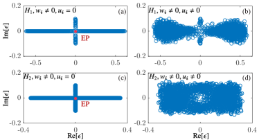
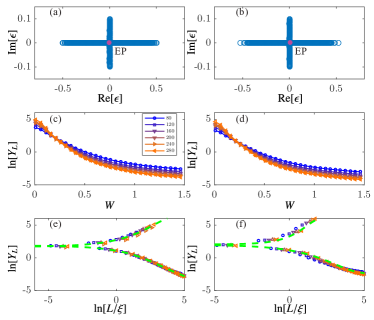
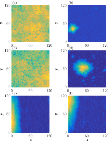
In addition to PTS, has PPHS as well, i.e., , such that are symmetric to the origin of the complex-energy plane. Disorders breaks lattice-translational symmetry but preserves PPHS since . Differently, PTS is preserved only if since and . Hence, for and , has both PTS and PPHS whose eigenvalues are in the cross region of the complex-energy plane and the EP is at the origin; while, for and , PTS is broken, and no EP is found, as shown in Figs. 1(a) and (b).
It is worth classifying the model within the framework of Altland-Zirnbauer (AZ) classification. In this symmetry classification, one require to consider TRS, PHS, particle-hole symmetry† (PHS†), time-reversal symmetry† (TRS†), chiral symmetry (CS), and sub-lattice symmetry (SLS), rather than PTS and PPHS, see Appendix A.3 for more details. For with , TRS, PHS, PHS†, TRS†, and SLS are broken but CS is preserved. Therefore, of belongs to class AIII. On the other hand, with breaks all symmetries of the AZ classification and belongs class A. We summarize these results in Table 2 of Appendix A.3.
The second model reads
| (2) |
where are the identity and the Pauli matrices acting on the pseudo-spin space. Disorders are modelled by the on-site term . The Bloch Hamiltonian of is , which has both PTS and PPHS, i.e., . Therefore, the complex-energy spectra of are symmetric to the origin of the complex-energy plane: with the EP at and standing for a two-fold degeneracy. With disorders, () preserves (breaks) PTS. Hence, with and has an EP at , and no EP is expected for and , see Figs. 1(c) and (d). Recall that the energy spectrum of is two-fold degenerated. Consequently, the EP shown in Fig. 1(c) is forth-order, different from the second-order EP in Fig. 1(a).
In addition to PTS and PPHS, has TRS, PHS, TRS†, and PHS† when and belongs to class DIII. Therefore, for , (class DIII) and (class AIII) belong to different symmetry classes in the AZ classification even though both of them have EPs. Differently, TRS and PHS† are broken if , and belongs to class DIII. A detailed analysis of symmetries is given in Appendix A.3 and the results are summarized in Table 2.
III Numerical methods
Complex mobility edge (complex energy at an ALT) can be numerically identified from the finite-size scaling analysis of the participation ratio of a state with energy defined as . Here, is the normalized wave function amplitude of a right eigenstate, and denotes the ensemble-average. scales with the system length as for extended states and approaches a constant for localized states [7]. If there is an ALT for a given state at a critical disorder , near behaves as
| (3) |
with being the fractal dimension [39] of the critical wave function, being a positive constant, and being the exponent of irrelevant scaling parameters. is the correlation length and diverges as near with being the universal critical exponent. The validity of the single-parameter scaling Eq. (3) has been confirmed in both Hermitian [40, 41] and non-Hermitian systems [19, 25]. ALTs in the same universality class have identical critical exponents.
In our approach, is numerically computed through the exact diagonalizations by using the KWTANT package [42] and the SciPy library [43] on Python. Then, a chi-square fit of to the scaling function Eq. (3) is performed by a polynomial expansion [44] from which we obtain , , , , , and the unknown scaling functions and . All fittings have satisfactory goodness-of-fits . Curves for different sample size are used to identify an ALT by the following criteria: (i) increases (decreases) with for extended (localized) states. (ii) for different cross each other at . (iii) for different collapse to a smooth scaling function near .
Note that and cannot be diagonalized at the EP [28]. Instead, we calculate with being the nearest eigenvalue to the EPs and assume . This approximation should be valid in the thermodynamic limit and for extremely close to EPs, see Appendix B. For finite-size systems, there should be a critical length above which the critical exponent , obtained by scaling analysis of , keeps unchanged within numerical errors. Hence, the approximation should be acceptable for . We find for and . Numerical evidence is given in Appendix B.
IV Results
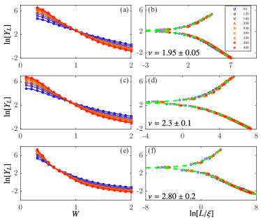
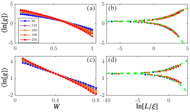
Let us first consider with , , and . The system has an EP at as shown in Fig. 1(a). Figure 2(a) shows of for various ranging from 80 to 400. Here, curves of different cross at a single point , and states of () are extended (localized) because increases (decreases) with . Finite-size scaling analysis yields , which is different from any known critical exponents of disordered non-Hermitian systems, indicating that the ALT belongs to an unknown universality class. Data near the critical point collapse on a single smooth scaling function with two branches for the extended and localized states, see Fig. 2(b).
For the state at energy in the symmetry-preserved phase, an ALT occurs at , see Fig. 2(c). The beautiful scaling function shown in Fig. 2(d) substantiates the criticality of the transition. The fitting suggests that which equals to that of Hermitian spinful Gaussian unitary ensemble [9], where TRS and spin-rotational symmetries are broken. This is because the non-Hermitian systems in the symmetry-preserved phase behave as the Hermitian systems and the disorder term breaks TRS, see Appendix A.3. Hence, the ALT shown in Figs. 2(c) and (d) belongs to the same universality class of the spinful Gaussian unitary class [9].
To further confirm the universality shown in Figs. 2(a)-(d), we carry out numerical calculations of the dimensionless conductance based on the transfer matrix method and perform the corresponding finite-size scaling analyse for (near the EP) and (the symmetry-preserved phase) of with , see Appendix D.1. The obtained critical exponents are and , respectively, which accord with those based on participation ratios within numerical errors. Besides, the critical exponent for the symmetry-preserved phase is also close to that for 2D Hermitian spinful Gaussian unitary ensemble [9], which is consistent with a recent work that estimates an equivalent mapping between the universality of class AIII for Hermitian systems and class A for non-Hermitian systems [25].
An ALT also occurs at for the state at in the symmetry-broken phase, as shown in Appendix D.3. The calculated critical exponent, , equals to that of within numerical errors, indicating that they have the same universality. The same universality of the symmetry-preserved and symmetry-broken phases can be understood as follows: The symmetry-preserved phase of with can be mapped into the symmetry-broken phase under the transformation due to the presence of both PTS and PPHS. The critical exponents of and should be the same since this mapping exchange only real and imaginary axes without changing their eigenfunctions.
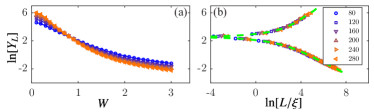
For , PTS is broken, and the EP disappears. Below, we set that both and uniformly distribute in . For a state at , an ALT can be identified at , see Figs. 2(e) and (f). The critical exponent is that is significantly different from those in Figs. 2(a)-(d), i.e., a distinguished universality class. From the best of our knowledge, there is no estimation of for non-Hermitian systems with PPHS in 2D. Remarkably, the obtained is very close to those of classes AIII, CII†, and DIII within the AZ classification [25].
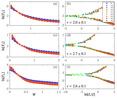
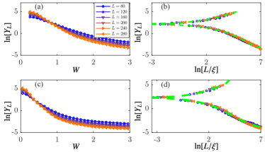
Now, let us turn to with that belongs to class DIII. Similar to , there is an ALT at for states near the EP, see Figs. 3(a) and (b). The critical exponent , the same as that of at the EP within numerical errors even though and with belong to different symmetry classes (class A and DIII, respectively) and the orders of EPs are different. Our results, presented in Figs. 2 and 3, suggest that ALTs for the states at EPs have the same critical exponent . This notion of “superuniversality” reminisces similar concept in disordered Hermitian superconducting systems [46].
To understand critical properties of ALTs for the symmetry-preserved states of , state of is studied. As shown in Figs. 3(c) and (d), an ALT occurs at with which is significantly larger than that shown in Figs. 2(c) and (d), but the same as that of 2D Gaussian sympletic ensembles in Hermitian random matrices [12]. Different from that breaks TRS, is invariant under the time-reversal transformation of , i.e., . This explains why the critical exponents of the symmetry-preserved states of fall into the universality class of [12] for the Hermitian time-reversal-invariant systems with .
Interestingly, of and , whose eigenvalues are complex, has different critical exponent as those above and thus belongs to a different universality class. This claim is derived from data of for distributing uniformly in the range of , as shown in Figs. 3(e) and (f), where an ALT happens at with . Thus, for systems without EPs, its universality class depends on symmetries, the same as their Hermitian counterparts.
V Discussions
Fractal dimension.Equation (3) says at criticality, in contrast to for extended states and for localized states. The fractal dimension is universal according to the renormalization-group theory of the model in dimensions [47]. At EPs, we obtain within numerical errors (see Tables in Appendix C) that supports this argument.
relates to the spectral compressibility characterizing fluctuations of the energy level number in an energy window near the criticality, i.e., . For Hermitian systems, the following relation between and holds: [48]. Therefore, our results suggest a universal for EPs. In an early work, we have shown that the nearest-neighbor level-spacing distributions follow some universal functions near EPs [38]. However, how to generate the concept of the spectral compressibility and test the correctness of remains unclear and deserves further studies.
More evidence for the superuniversality at EPs.The meaning of universality requires the independence of on the boundary conditions and the forms of disorders [4]. Since open boundary conditions and uniform distributions of random numbers are used in Figs. 2 and 3, studies with periodical boundary condition and disorders of the normal-distribution are carried out to test the universality of at EPs, see Appendices D.3 and D.4. Indeed, the same critical exponents for EPs, , is obtained in all cases.
Skin effect.The non-Hermiticity itself can also lead to localizations of waves. A phenomenon is known as the non-Hermitian skin effect where the wave functions localize at the boundary of systems for some specific non-Hermiticities [15]. However, our models, Eqs. (1) and (2) with PTS, do not suffer from the skin effect such that all localizations shown here are due to disorders rather than non-Hermiticities, see Appendix E.
Materials relevance.The participation ratio of a non-Hermitian Hamiltonian with a right eigenenergy is the same as of with being the identity matrix of the same dimension of . For , one can easy to find that . By definition, . Hence, additional on-site potentials and to Hamiltonians Eq. (1) and (2) do not change the participation ratios, as well as the universality.
Note that the effective Hamiltonian of near reads , which, together with a non-local loss with , which does not affect the criticality, describes a Rashba spin-orbit coupling with different spin lifetimes. Possible physical realizations of are ferromagnetic semiconductors such as MnGaAs and other III-V host materials [49] with a spin-dependence impurity that breaks TRS. Likewise, can be treated as the 2D electron gases with Rashba spin-orbit coupling and different lifetimes of spins/pseudo-spins, but the disorders are spin-independent.
In addition to electronic systems, EPs present in many other systems, including lasers [50, 51], micro-cavities [52], electrics [53], and magnonics [29], to name a few. Disorders can be artificially induced in such systems such that the ALTs of the EPs in these systems can be experimentally studied in principle. In Appendix F, a laser cavity network is proposed as a possible experimental verification of the numerical results presented in this paper.
VI Conclusion
In summary, ALTs at EPs of two non-Hermitian systems of different symmetries have the same critical exponent , independent of the forms of disorders and the boundary conditions. This strongly suggests that ALTs at EPs of non-Hermitian systems belong to a new universality class that may depends only on dimensionality. Besides, the universality of ALTs of the symmetry-preserved and symmetry-broken phase is the same as their Hermitian counterpart and depends on the presence of their symmetries.
Acknowledgements.
This work is supported by the National Natural Science Foundation of China (Grants No. 11704061 and No. 11974296) and Hong Kong RGC (Grants No. 16300522 and No. 16302321).Appendix A Symmetry classifications
In Appendix A.1, definitions of parity-time and parity-particle-hole symmetries are first presented and explained. Then, their constraints on the energy spectra are derived, especially for those non-Hermitian systems given in Appendix A.2. Finally, we identify the symmetry classes of and in Appendix A.3.
A.1 Parity-time and parity-particle-hole symmetries
A system characterized by Hamiltonian is said to have time-reversal symmetry (TRS) if
| (4) |
in the real space, or
| (5) |
in the momentum space. Here, . The system is said to have parity-time symmetry (PTS) if does not change under a combination of time-reversal and parity inversion transformations. For single particle Hamiltonians in the real space, the parity operator can be written as with and representing spatial inversion on lattice, i.e, goes to . Consequently, the parity-inversion transformation changes to for Bloch Hamiltonians in the momentum space. Then, we say a non-Hermitian system with PTS if
| (6) |
in the real space, or
| (7) |
in the momentum space. By introducing the operator that changes to , we can write Eqs. (5) and Eq. (7) in elegant forms as and , respectively.
In addition to PTS, our non-Hermitian models and also have parity-particle-hole symmetry (PPHS), a symmetry relating to the product of particle-hole and parity-inversion transformations. We first define particle-hole symmetry (PHS) for non-Hermitian systems:
| (8) |
in the real space, or
| (9) |
in the momentum space with and . Similar to PTS, we say a non-Hermitian system has PPHS if
| (10) |
in the real space, or
| (11) |
in the momentum space. In Eqs. (10) and (11), and . Likewise, Eqs. (9) and (11) can be rewritten as and , respectively. Here, is the transpose operator. We summarize the definition of TRS, PTS, PHS, and PPHS in Table 1.
| symmetry | real space | momentum space |
|---|---|---|
| TRS | ||
| PTS | ||
| PHS | ||
| PPHS |
Before the end of this section, we would like to emphasize that disordered non-Hermitian Hamiltonians are defined in the real space rather than the momentum space, and one can calculate the corresponding Bloch Hamiltonian only in the clean limit. A disordered non-Hermitian system’s Hamiltonian with a symmetry guarantees that its Bloch Hamiltonian is also invariant with the corresponding symmetry operation, but it is not vice versa since disorders may break the symmetry.
A.2 Constraints of complex energies due to symmetries
PTS gives some constraints on the complex eigenenergies. Let us assume a Bloch Hamiltonian has PTS, i.e., Eq. (7), and is a right eigenstate of with an eigenenergy , i.e., . Then,
| (12) |
Equation (12) means that is also a right eigenstate of with eigenenergy . If the two states and are the same, , i.e., is real. This can happen for either or if has a double degeneracy [38].
PPHS also gives constraints on the complex eigenenergies. Recall that PPHS is defined as in the momentum space, where is the transpose operator satisfying with being arbitrary complex number, operator, and ket, respectively. For a corresponding left eigenstate of satisfying ,
| (13) |
To derive Eq. (13), we have used by taking the complex conjugate of Eq. (11). Multiply to Eq. (13):
| (14) |
Therefore, there always exists a right eigenstate with energy . Namely, PPHS makes the complex-energy spectrum symmetric to the origin of the complex-energy plane.
A.3 Symmetry classification
Altland-Zirnbauer (AZ) classification is a well-established approach to determine the symmetry class of a non-Hermitian system [21]. Noticeably, our models and go beyond the AZ classification due to the presence of PTS and PPHS shown in Table 1. However, we would like to determine the symmetry classes of our models within the framework of AZ classification. TRS and PHS are two symmetries in the AZ classification. In addition, one require time-reversal symmetry† (TRS†), particle-hole symmetry† (PHS†), chiral symmetry (CS), and sub-lattice symmetry (SLS). TRS† is defined as
| (15) |
PHS† is defined as
| (16) |
CS is defined as
| (17) |
and SLS is defined as
| (18) |
CS and SLS can be treated as combinations of PHS and TRS† and PHS and TRS, respectively. On the one hand, if none of TRS, PHS, PHS†, and TRS† are preserved, one requires to determine whether the non-Hermitian system has CS and SLS. On the other hand, if all TRS, PHS, PHS†, and TRS† are preserved, CS and SLS are solely determined.
Let us determine the symmetry class of . Note that
| (19) |
| (20) |
and
| (21) |
From Eqs. (19) and (20), one can see the hopping terms of and are the same since the non-Hermiticity is introduced by the on-site terms. For (see Fig. 1(b)), TRS, PHS, TRS†, PHS†, and SLS are broken, but CS is preserved with and . Here, is the unit matrix acting on the coordinate subspace. Hence, belongs to class AIII. For (see Fig. 1(a)), belongs to class A, where TRS, PHS, TRS†, PHS†, CS, and SLS are broken.
also has PTS and PPHS. Note that
| (22) |
To derive Eq. (22), we have reversed the and axes. Effectively, keeps the on-site terms but takes the complex-conjugate of the coefficients of the hopping terms. For , we can choose such that Eq. (8) is satisfied. One can also use an elegant form of to write the parity-time operator. Differently, one cannot find a proper for . Hence, PTS is preserved only if . On the other hand,
| (23) |
One can always choose such that PPHS is preserved.
| TRS | PHS | TRS† | PHS† | CS | SLS | class | PTS | PPHS | Hermitian class | |
|---|---|---|---|---|---|---|---|---|---|---|
| 0 | 0 | 0 | 0 | 1 | 0 | AIII | 1 | -1 | A | |
| 0 | 0 | 0 | 0 | 0 | 0 | A | 0 | -1 | AIII | |
| TRS | PHS | TRS† | PHS† | CS | SLS | class | PTS | PPHS | Hermitian class | |
| -1 | 1 | -1 | -1 | 1 | 1 | DIII | 1 | -1 | AII | |
| 0 | 1 | -1 | 0 | 0 | 1 | DIII | 0 | -1 | DIII | |
Now, let us turn to . Note that
| (24) |
and
| (25) |
For (see Fig. 1(c)), TRS, PHS, TRS†, and PHS† are preserved with . Now, belongs to class DIII. On the other hand, for (see Fig. 1(d)), TRS and PHS† are broken since the on-site terms are complex. In this case, belongs to class DIII.
also has PTS and PPHS. Note that
| (26) |
and
| (27) |
For of , PTS and PPHS are preserved with and . For , PTS is broken but PPHS is still preserved. We summarize the presence/absence of PTS and PPHS for and in Table 2.
Before the end of this section, we want to mention that of also has pseudo-Hermitian symmetry which is defined as
| (28) |
in the real space, or
| (29) |
in the momentum space. Here, , and . One can choose to satisfy Eq. (28). Pseudo-Hermitian symmetry is equivalent to the AZ or AZ† classes with SLS, see Ref. [21] for more details. Therefore, does not have pseudo-Hermitian symmetry due to the absence of SLS.
Appendix B Nearest-neighbor levels to EPs
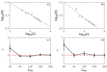
Since the non-Hermitian Hamiltonians cannot be exactly diagonalized at the EPs, we find the nearest-neighbor level to the EPs (locating at for our models and ) and treat the participation ratio of , say , as numerically. Here, we show that become extremely close to the EP for such that, for large enough sizes, . To support this argument, we plot the ensemble-average as a function of system size for and with and , see Figs. 4(a) and (b), respectively. Since the EP locates at , is the distance between the EP and its nearest-neighbor level. As we can see, scales with as with for and for , i.e., in both cases, .
Our numerical results also show that one cannot use very small system sizes to determine the critical exponents of EPs of and , i.e., a large enough size to ensure close to the EPs. We find that the critical exponent decreases with for relatively small size but becomes constant upon a critical length . Figures 4(c,d) show the critical exponents for as a function of obtained by finite-size scaling analyses of sizes with . It is seen that the critical exponent approaches to within numerical errors for .
Appendix C Finite-size scaling analysis and fitting parameters
To determine the critical exponent , a finite-size scaling analysis of participation ratio is required. Near the critical disorder , scales with the system size as
| (30) |
with the correlation length diverging at . We expand the unknown scaling function and as
| (31) |
with
| (32) |
The fitting parameters are (in total, there are fitting parameters) with being the fractal dimension, being the critical exponent of correlation length, being the critical disorder, and being the exponent of the irrelevant variable. The maximal likelihood estimate of the fitting parameters is obtained by minimizing the following quantity:
| (33) |
Here, are the numerical data, and are given by the scaling function Eq. (30). is known as the chi-square. The total degree of freedom for a fitting process is . We also estimate the so-called goodness-of-fit by following the standard scenario, which can be used to judge whether the fitting is acceptable or not. Generally speaking, a wrong model will often been rejected with a very small values of ; while it is acceptable if [44].
| disorders | |||||||
|---|---|---|---|---|---|---|---|
| 0 | 139 | 0.1 | |||||
| -0.2 | 139 | 0.2 | |||||
| 0.08i | 139 | 0.1 | |||||
| -0.2+0.01i | 127 | 0.05 |
| disorders | |||||||
|---|---|---|---|---|---|---|---|
| 0 | 121 | 0.08 | |||||
| -0.2 | 139 | 0.03 | |||||
| -0.2+0.01i | 139 | 0.1 |
| disorders | ||||||||
|---|---|---|---|---|---|---|---|---|
| 0 | 139 | 0.3 | ||||||
| 0 | 133 | 0.1 |
| disorders | ||||||||
|---|---|---|---|---|---|---|---|---|
| 0 | 139 | 0.1 | ||||||
| 0 | 139 | 0.02 |
Appendix D More evidence for the universality
Here, we give more data to support the universality at EPs. In Appendix D.1, we study the ALTs of with by calculating the dimensionless conductances based on the transfer matrix method [45]. The obtained critical exponent is identical to that by participation ratios, a strong support to the universality of ALTs in Figs. 2(a)-(d). In Appendix D.2, we numerically study the ALTs in the symmetry-broken phases. In Appendices D.3 and D.4, we study the ALTs under a different boundary condition and with a different form of disorders. All ALTs near the EPs in Appendices D.2, D.3, and D.4 have the same criticality.
D.1 Dimensionless conductance
As a self-consistent check, we investigate the localization properties of states of with through the data of dimensionless conductance. By using the transfer matrix method [45], we calculate the dimensionless conductance of a disordered sample modelled by Eq. (1) between two clean semi-infinite leads by Eq. (1) with at a complex Fermi level , i.e., with being the transmission matrix. As the standard paradigm, the contact resistance is eliminated. For a given disorder , the localization nature of a state at are determined by the following criteria: (i) increases (decreases) with the size for the state being extended (localized); while is size-independent for the critical state. (ii) If there exists a quantum phase transition at a critical disorder , of different size near collapse into a smooth scaling curve with the correlation length diverging as .
The ensemble-average as a function of for (near the exceptional point) and (in the symmetry-preserved phase) for are displayed in Figs. 5(a,c), respectively. It should be noted that it is unreasonable to choose in the transfer matrix approach since cannot be diagonalized at the exception point [28]. Instead, we choose a state at , which is very close to the EP, and find a transition from extended states to localized states at . Finite-size scaling analysis gives , which equals to from the data of participation ratios within numerical errors. The details of the finite-size scaling analyses can be found in the Appendix of Ref. [44]. On the other hand, for (in the symmetry-preserved phase), we also see a critical point at near which with , which equals to shown in Fig. 2(d). Hence, the obtained critical exponents by transfer matrix methods are consistent as those from participation ratios, which should be strong supports to the universality.
D.2 ALT in the symmetry-broken phase
For a full picture for the localization nature of states of the non-Hermitian model , we also calculate the ensemble average as a function of for various , as we do in Figs. 2(a)-(d), but for one state in the symmetry-broken phase (). The obtained data are displayed in Fig. 3. Clearly, data for different sizes cross at one point and those of () increases (decreases) with the system size . These features indicate a transition from a band extended states to a band of localized states at . ALTs can not only happen near the EP and in the symmetry-preserved phase as shown in Figs. 2(a)-(d) but also in the symmetry-broken phase, where the eigenenergies come as the complex-conjugate pairs .
To further substantiate the criticality, we perform the finite-size scaling analysis for data in Fig. 3(a). Our analysis shows that the correlation lengths diverge as with , and data of as a function of collapse to two different curves (the upper and lower branches are for extended and localized states, respectively). The critical exponent equals to that of in the symmetry-preserved phase. As we explained in the main text, ALTs of the symmetry-preserved and symmetry-broken phases belong to the same universality class. Numerical data in Fig. 2(c,d) and Fig. 6 confirm this assertion.
D.3 ALTs under periodic boundary conditions
In Figs. 2 and 3, we apply open boundary conditions to the 2D Hamiltonians and . Here, we change the boundary condition to periodic boundary conditions and see whether the critical exponent is different for (EPs). The calculated as a function of for with is depicted in Fig. 7(a) with a critical disorder at . The finite size scaling analysis yields . Likewise, we find the ALT at with the critical exponent , see Fig. 7(c). Hence, the universality at EPs are not affected by choosing a different boundary condition. The scaling functions are shown in Figs. 7(c) and (d). Other fitting parameters are in Table 5.
D.4 ALTs for Gaussian distributions
In Figs. 2 and 3, we model disorders of and by random on-site potentials, whose amplitudes and distribute independently and uniformly in a range of . Here, we supply numerical evidence to the universality at EPs for a different form of randomness, i.e., and are white-noise and follow the Gaussian distribution of zero mean and variance . We label the corresponding Hamiltonians as and , whose Bloch Hamiltonians are the same as those of and and the disordered on-site potentials are Gaussian. Since we focus on delocalization-localization transitions at EPs, we set in what follows.
Similar to and , eigenenergies of and form crosses in the complex-energy plane with the second-order and fourth-order EPs locating at . These features are visualized in Figs. 8(a) and (b) for . We then investigate the Anderson localization transitions at the EPs. The calculated are shown in Figs. 8(c) and (d) for and , respectively. Finite-size scaling analyse yield for and for , which are identical to those of and within numerical errors. The scaling functions are given in Figs. 8(e) and (f).
Appendix E Skin effect
Non-Hermiticities sometimes cause a skin effect where the wave functions localize exponentially at boundaries of systems of the open boundary conditions. This can be seen by the following low-energy continuous Hamiltonian
| (34) |
with and being real numbers. The Hermitian part of Eq. (34) is the effective Hamiltonian of the Hermitian part of model (1) of the main text, and is a general non-Hermitian potential. One can generalize the Hamiltonian in the real space to that in the complex space, i.e.,
| (35) |
with being complex numbers. The role of can be thus seen by replacing the real wave vectors by the complex ones in the Bloch phase of . Hence, eigenstates of Eq. (35) localized exponentially at the boundaries if . However, this never happens for the non-Hermitian systems with either PTS or pseudo-Hermitian symmetry. For PTS, one requires . Since
| (36) |
we must set and choose . Likewise, one can find that the skin effect is prohibited for a pseudo-Hermitian system.
This can be seen in the following. In Fig. 9(a), we show the wave function distribution for , whose EPs are second-order, at a particular disorder . One can see that the wave function spreads over the whole sample since it is a delocalized state. On the other hand, for a stronger disorder that is larger than (see Table 3), the state is highly localized at the bulk, see Fig. 9(b). Similar features are also observed for , see Figs. 9(c) and (d). Noticeably, such localizations are different from that due to the skin effect. To see it, we consider the following two models:
| (37) |
and
| (38) |
The differences between Eqs. (37) and (38) and and are the non-Hermitian on-site potentials: They are and in Eqs. (37) and (38) but and in and . The modifications of the non-Hermitian potentials lead to the skin effect in the direction such that wave functions of the two new models localized exponentially, see Figs. 9(e) and (f). Such localizations are intrinsically different from Anderson localizations where wave functions can be localized at the bulk, rather than the edges, of a non-Hermitian system.
Appendix F Honeycomb laser cavity network
One possibility is to model Haldane Hamiltonian by the laser cavity network as recently done in experiments that realized chiral edge states [50, 51]. In an early work [16], we derived the effective Hamiltonian of coupled laser cavities on a honeycomb lattice
| (39) |
Here, and are the laser field amplitudes at site of A and B sub-lattices, respectively. and denote the nearest-neighbor sites and the next-nearest-neighbor sites, respectively. Each resonator is coupled to its nearest-neighbors sites with a real coupling constant and to its next-nearest-neighbor sites with a complex coupling constant with being the tunable Haldane flux parameters. The complex parameters and are
| (40) |
and
| (41) |
Real numbers and represent the resonance frequencies of the resonator at site of A and B sub-lattices. The resonance frequency depend on the size and the shape of the resonator. Therefore, disorders can be introduced by setting and randomly. The real positive number is the linear loss of a resonator. Real positive number and in Eqs. (40) and (41) are the optical gains via stimulated emission that is inherently saturated. Hereafter, we choose
| (42) |
such that .
In the absence of disorders, say , Eq. (39) can be block diagonalized in the momentum space
| (43) |
where
| (44) |
with
| (45) |
Note that stand for the unit matrix and the Pauli matrices acting on the A-B sub-lattice space. In Eq. (45), , and . The Hermitian part of Eq. (45) supports chiral edge states for and and . Near the two distinct corners and , we can expand the Bloch Hamiltonian with small :
| (46) |
with the subscripts standing for the and , respectively. By artificially tuning , Eq. (46) is invariant under parity-time operation, i.e., , and supports an EP at .
An on-site randomness like can be achieved by artificially changing the resonant frequencies of the cavities. In principle, one can measure the laser field amplitudes of Eq. (39), see Ref. [51], from which the participation ratio can be calculated . The ALTs can be seen by studying the size-dependence of near the EP, and the critical exponent can be calculated through the finite-size scaling analysis. We thus expect the designed laser cavity networks are ideal platform to study the Anderson localization transitions at EPs and all conclusion given in this work can be experimentally tested based on the laser cavity networks.
References
- [1] P. W. Anderson, Absence of Diffusion in Certain Random Lattices, Phys. Rev. 109, 1492 (1958).
- [2] P. A. Lee and T. V. Ramakrishnan, Disordered electronic systems, Rev. Mod. Phys. 57, 287 (1985).
- [3] B. Kramer, and A. MacKinnon, Localization: theory and experiment, Rep. Prog. Phys. 56, 1469 (1993).
- [4] F. Evers and A. D. Mirlin, Anderson transitions, Rev. Mod. Phys. 80, 1355 (2008).
- [5] H. Levine, S. B. Libby, and A. M. M. Pruisken, Theory of the quantized Hall effect (I), Nucl. Phys. B 240, 30 (1984); Theory of the quantized hall effect (II), 240, 49 (1984); Theory of the quantized Hall effect (III), 240, 71 (1984).
- [6] B. Huckestein, Scaling theory of the integer quantum Hall effect, Rev. Mod. Phys. 67, 357 (1995).
- [7] C. Wang, Y. Su, Y. Avishai, Y. Meir, and X. R. Wang, Band of Critical States in Anderson Localization in a Strong Magnetic Field with Random Spin-Orbit Scattering, Phys. Rev. Lett. 114, 096803 (2015).
- [8] Y. Su, C. Wang, Y. Avishai, Y. Meir, and X. R. Wang, Absence of localization in disordered two-dimensional electron gas at weak magnetic field and strong spin-orbit coupling, Sci. Rep. 6, 33304 (2016).
- [9] C. Wang and X. R. Wang, Anderson transition of two-dimensional spinful electrons in the Gaussian unitary ensemble, Phys. Rev. B 96, 104204 (2017).
- [10] S. N. Evangelou, Anderson Transition, Scaling, and Level Statistics in the Presence of Spin Orbit Coupling, Phys. Rev. Lett. 75, 2550 (1995).
- [11] R. Merkt, M. Janssen, and B. Huckestein, Network model for a two-dimensional disordered electron system with spin-orbit scattering, Phys. Rev. B 58, 4394 (1998).
- [12] Y. Asada, K. Slevin, and T. Ohtsuki, Anderson Transition in Two-Dimensional Systems with Spin-Orbit Coupling, Phys. Rev. Lett. 89, 256601 (2002).
- [13] T. E. Lee, Anomalous Edge State in a Non-Hermitian Lattice, Phys. Rev. Lett. 116, 133903 (2016).
- [14] F. K. Kunst, E. Edvardsson, J. C. Budich, and E. J. Bergholtz, Biorthogonal Bulk-Boundary Correspondence in Non-Hermitian Systems, Phys. Rev. Lett. 121, 026808 (2018).
- [15] S. Yao and Z. Wang, Edge States and Topological Invariants of Non-Hermitian Systems, Phys. Rev. Lett. 121, 086803 (2018).
- [16] C. Wang and X. R. Wang, Hermitian chiral boundary states in non-Hermitian topological insulators, Phys. Rev. B 105, 125103 (2022).
- [17] N. Hatano and D. R. Nelson, Localization Transitions in Non-Hermitian Quantum Mechanics, Phys. Rev. Lett. 77, 570 (1996).
- [18] Y. Huang and B. I. Shklovskii, Anderson transition in three-dimensional systems with non-Hermitian disorder, Phys. Rev. B 101, 014204 (2020).
- [19] C. Wang and X. R. Wang, Level statistics of extended states in random non-Hermitian Hamiltonians, Phys. Rev. B 101, 165114 (2020).
- [20] D. Bernard and A. LeClair, A Classification of Non-Hermitian Random Matrices, arXiv:cond-mat/0110649.
- [21] K. Kawabata, K. Shiozaki, M.Ueda, and M. Sato, Symmetry and Topology in Non-Hermitian Physics, Phys. Rev. X 9, 041015 (2019).
- [22] X. Luo, T. Ohtsuki, and R. Shindou, Universality Classes of the Anderson Transitions Driven by Non-Hermitian Disorder, Phys. Rev. Lett. 126, 090402 (2021).
- [23] K. Kawabata and S. Ryu, Nonunitary Scaling Theory of Non-Hermitian Localization, Phys. Rev. Lett. 126, 166801 (2021).
- [24] X. Luo, T. Ohtsuki, and R. Shindou, Transfer matrix study of the Anderson transition in non-Hermitian systems, Phys. Rev. B 104, 104203 (2021).
- [25] X. Luo, Z. Xiao, K. Kawabata, T. Ohtsuki, and R. Shindou, Unifying the Anderson transitions in Hermitian and non-Hermitian systems, Phys. Rev. Research 4, L022035 (2022).
- [26] C. M. Bender and S. Boettcher, Real Spectra in Non-Hermitian Hamiltonians Having Symmetry, Phys. Rev. Lett. 80, 5243 (1998).
- [27] A. Mostafazadeh, Pseudo-Hermiticity versus PT Symmetry: The Necessary Condition for the Reality of the Spectrum of a Non-Hermitian Hamiltonian, J. Math. Phys. (N.Y.) 43, 205 (2002); Pseudo-Hermiticity versus PT Symmetry II: A Complete Characterization of Non-Hermitian Hamiltonians with a Real Spectrum, J. Math. Phys. (N.Y.) 43, 2814 (2002); Pseudo-Hermiticity versus PT Symmetry III: Equivalence of Pseudo-Hermiticity and the Presence of Antilinear Symmetries, J. Math. Phys. (N.Y.) 43, 3944 (2002).
- [28] W. D. Heiss, The Physics of Exceptional Points, J. Phys. A 45, 444016 (2012).
- [29] H. Yang, C. Wang, T. Yu, Y. Cao, and P. Yan, Antiferromagnetism Emerging in a Ferromagnet with Gain, Phys. Rev. Lett. 121, 197201 (2018).
- [30] Z. Xiao, H. Li, T. Kottos, and A. Alù, Enhanced Sensing and Nondegraded Thermal Noise Performance Based on -Symmetric Electronic Circuits with a Sixth-Order Exceptional Point, Phys. Rev. Lett. 123, 213901 (2019).
- [31] Ş. K. Özdemir, S. Rotter, F. Nori, and L. Yang, Parity-Time Symmetry and Exceptional Points in Photonics, Nat. Mater. 18, 783 (2019).
- [32] M.-A. Miri and A. Alù, Exceptional Points in Optics and Photonics, Science 363, eaar7709 (2019).
- [33] S. Malzard, C. Poli, and H. Schomerus, Topologically Protected Defect States in Open Photonic Systems with Non-Hermitian Charge-Conjugation and Parity-Time Symmetry, Phys. Rev. Lett. 115, 200402 (2015).
- [34] D. Leykam, K. Y. Bliokh, C. Huang, Y. D. Chong, and F. Nori, Edge Modes, Degeneracies, and Topological Numbers in Non-Hermitian Systems, Phys. Rev. Lett. 118, 040401 (2017).
- [35] Y. Xu, S.-T. Wang, and L.-M. Duan, Weyl Exceptional Rings in a Three-Dimensional Dissipative Cold Atomic Gas, Phys. Rev. Lett. 118, 045701 (2017).
- [36] K. Kawabata, T. Bessho, and M. Sato, Classification of Exceptional Points and Non-Hermitian Topological Semimetals, Phys. Rev. Lett. 123, 066405 (2019).
- [37] X.-X. Zhang and M. Franz, Non-Hermitian Exceptional Landau Quantization in Electric Circuits, Phys. Rev. Lett. 124, 046401 (2020).
- [38] C. Wang and X. R. Wang, Linear level repulsions near exceptional points of non-Hermitian systems, Phys. Rev. B 106, L081118 (2022).
- [39] X. R. Wang, Y. Shapir, and M. Rubinstein, Analysis of multiscaling structure in diffusion-limited aggregation: A kinetic renormalization-group approach, Phys. Rev. A 39, 5974 (1989).
- [40] J. H. Pixley, P. Goswami, and S. Das Sarma, Anderson Localization and the Quantum Phase Diagram of Three Dimensional Disordered Dirac Semimetals, Phys. Rev. Lett. 115, 076601 (2015).
- [41] C. Wang, P. Yan, and X. R. Wang, Non-Wigner-Dyson level statistics and fractal wave function of disordered Weyl semimetals, Phys. Rev. B 99, 205140 (2019).
- [42] C. W. Groth, M. Wimmer, A. R. Akhmerov, and X. Waintal, Kwant: A software package for quantum transport, New J. Phys. 16, 063065 (2014).
- [43] P. Virtanen, R. Gommers, T. E. Oliphant, M. Haberland, T. Reddy, D. Cournapeau, E. Burovski, P. Peterson, W. Weckesser, J. Bright et al., SciPy 1.0: Fundamental algorithms for scientific computing in Python, Nat. Methods 17, 261 (2020).
- [44] W. Chen, C. Wang, Q. Shi, Q. Li, and X. R. Wang, Metal to marginal-metal transition in two-dimensional ferromagnetic electron gases, Phys. Rev. B 100, 214201 (2019).
- [45] A. MacKinnon and B. Kramer, The scaling theory of electrons in disordered solids: Additional numerical results, Z. Phys. B 53, 1 (1983).
- [46] I. A. Gruzberg, N. Read, and S. Vishveshwara, Localization in disordered superconducting wires with broken spin-rotation symmetry, Phys. Rev. B 71, 245124 (2005).
- [47] F. Wegner, Inverse participation ratio in dimensions, Z. Phys. B 36, 209 (1980).
- [48] F. Evers and A. D. Mirlin, Fluctuations of the Inverse Participation Ratio at the Anderson Transition, Phys. Rev. Lett. 84, 3690 (2000).
- [49] N. Nagaosa, J. Sinova, S. Onoda, A. H. MacDonald, and N. P. Ong, Anomalous Hall effect, Rev. Mod. Phys. 82, 1539 (2010).
- [50] G. Harari, M. A. Bandres, Y. Lumer, M. C. Rechtsman, Y. D. Chong, M. Khajavikhan, D. N. Christodoulides, and M. Segev, Topological insulator laser: Theory, Science 359, eaar4003 (2018).
- [51] M. A. Bandres, S. Wittek, G. Harari, M. Parto, J. Ren, M. Segev, D. Christodoulides, and M. Khajavikhan, Topological insulator laser: Experiments, Science 359, eaar4005 (2018).
- [52] B. Peng, Ş. K. Özdemir, F. Lei, F. Monifi, M. Gianfreda, G. L. Long, S. Fan, F. Nori, C. M. Bender, and L. Yang, Parity-Time-Symmetric Whispering-Gallery Microcavities, Nat. Phys. 10, 394 (2014).
- [53] V. V. Konotop, J. Yang, and D. A. Zezyulin, Nonlinear waves in -symmetric systems, Rev. Mod. Phys. 88, 035002 (2016).