GAGA: Deciphering Age-path of Generalized
Self-paced Regularizer

Abstract

Nowadays self-paced learning (SPL) is an important machine learning paradigm that mimics the cognitive process of humans and animals. The SPL regime involves a self-paced regularizer and a gradually increasing age parameter, which plays a key role in SPL but where to optimally terminate this process is still non-trivial to determine. A natural idea is to compute the solution path w.r.t. age parameter (i.e., age-path). However, current age-path algorithms are either limited to the simplest regularizer, or lack solid theoretical understanding as well as computational efficiency. To address this challenge, we propose a novel Generalized Age-path Algorithm (GAGA) for SPL with various self-paced regularizers based on ordinary differential equations (ODEs) and sets control, which can learn the entire solution spectrum w.r.t. a range of age parameters. To the best of our knowledge, GAGA is the first exact path-following algorithm tackling the age-path for general self-paced regularizer. Finally the algorithmic steps of classic SVM and Lasso are described in detail. We demonstrate the performance of GAGA on real-world datasets, and find considerable speedup between our algorithm and competing baselines.

1 Introduction

The SPL.

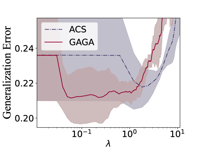
Figure 1: Learning curve against age $\lambda$. The curve is recorded when running linear regression on music dataset.

Self-paced learning (SPL) [1] is a classical learning paradigm and has attracted increasing attention in the communities of machine learning [2, 3, 4, 5, 6], data mining [7, 8] and computer vision [9, 10, 11]. The philosophy under this paradigm is simulating the strategy that how human-beings learn new knowledge. In other words, SPL starts learning from easy tasks and gradually levels up the difficulty while training samples are fed to the model sequentially. At its core, SPL can be viewed as an automatic variant of curriculum learning (CL) [12, 13], which uses prior knowledge to discriminate between simple instances and hard ones along the training process. Different from CL, the SPL assigns a real-valued “easiness weight” to each sample implicitly by adding a self-paced regularizer (SP-regularizer briefly) to the primal learning problem and optimizes the original model parameters as well as these weights. Considering this setting, the SPL is reported to alleviate the problem of getting stuck in bad local minima and provides better generalization as well as robustness for the models, especially in hard condition of heavy noises or a high outlier rate [1, 14].There are two critical aspects in SPL, namely the SP-regularizer and a gradually increasing age parameter. Different SP-regularizers can be designed for different kinds of training tasks. At the primary stage of SPL, only the hard SP-regularizer is utilized and leads to a binary variable for weighting samples [1]. Going with the advancing of the diverse SP-regularizers [15], SPL equipped with different types of SP-regularizers has been successfully applied to various applications [16, 3, 17]. As for the age parameter (a.k.a. pace parameter), the users are expected to increase its value continually under the SPL paradigm, given that the age parameter represents the maturity of current model. A lot of empirical practices have turned out that seeking out an appropriate age parameter is crucial to the SPL procedure [18]. The SPL tends to obtain a worse performance in the presence of noisy samples/outliers when the age parameter gets larger, or conversely, an insufficient age parameter makes the gained model immature (i.e. underfitting. See Figure 1).

On the age-path of SPL.

Although the SPL is a classical and widespread learning paradigm, when to stop the increasing process of age parameter in implementation is subject to surprisingly few theoretical studies. In the majority of practices [19], the choice of the optimal model age has, for the time being, remained restricted to be made by experience or by using the trial-and-error approach, which is to adopt the alternate convex search (ACS) [20] multiple times at a predefined sequence of age parameters. This operation is time-consuming and could miss some significant events along the way of age parameter. In addition, the SPL regime is a successive training process, which makes existing hyperparameter tuning algorithms like parallelizing sequential search [21] and bilevel optimization [22] difficult to apply. Instead of training multiple subproblems at different age parameters, a natural idea is to calculate the solution path about age parameter, namely age-path (e.g., see Figure 2). A solution path is a set of curves that demonstrate how the optimal solution of a given optimization problem changes w.r.t. a hyperparameter. Several papers like [23, 24] laid the foundation of solution path algorithm in machine learning by demonstrating the rationale of path tracking, which is mainly built on the Karush-Khun-Tucker (KKT) theorem [25]. Existing solution path algorithms involve generalized Lasso [26], semi-supervised support vector classification [27], general parametric quadratic programming [28], etc. However, none of the existing methods is available to SPL regime because they are limited to uni-convex optimization while the SPL objective is a biconvex formulation. Assume we’ve got such an age-path, we can observe the whole self-paced evolution process clearly and recover useful intrinsic patterns from it.

State of the art.

Yet, a rapidly growing literature [29, 19, 30, 31] is devoted to developing better algorithms for solving the SPL optimization with ideas similar to age-path. However, despite countless theoretical and empirical efforts, the understanding of age-path remains rather deficient. Based on techniques from incremental learning [32], [31] derived an exact age-path algorithm for mere hard SP-regularizer, where the path remains piecewise constant. [29, 30] proposed a multi-objective self-paced learning (MOSPL) method to approximate the age-path by evolutionary algorithm, which is not theoretically stable. Unlike previous studies, the difficulty of revealing the exact generalized age-path lies in the continuance of imposed weight and the alternate optimization procedure used to solve the minimization function. From this point of view, the technical difficulty inherent in the study of age-path with general SP-regularizer is intrinsically more challenging.

Proposed Method.

In order to tackle this issue, we establish a novel Generalized Age-path Algorithm (GAGA) for various self-paced regularizers, which prevents a straightforward calculation of every age parameter. Our analysis is based on the theorem of partial optimum while previous theoretical results are focused on the implicit SPL objective. In particular, we enhance the original objective to a single-variable analysis problem, and use different sets to partition samples and functions by their confidence level and differentiability. Afterward, we conduct our main theorem results based on the technique of ordinary differential equations (ODEs). In the process, the solution path hits, exits, and slides along the various constraint boundaries. The path itself is piecewise smooth with kinks at the times of boundary hitting and escaping. Moreover, from this perspective we are able to explain some shortcomings of conventional SPL practices and point out how we can improve them. We believe that the proposed method may be of independent interest beyond the particular problem studied here and might be adapted to similar biconvex schemes.

Contributions.

Therefore, the main contributions brought by this work are listed as follows.

• We firstly connect SPL paradigm to the concept of partial optimum and emphasize its importance here that has been ignored before, which gives a novel viewpoint to the robustness of SPL. Theoretical studies are conducted to reveal that our result does exist some equivalence with previous literature, which makes our study more stable.

• A framework of computing the exact age-path for generalized SP-regularizer is derived using the technique of ODEs, which allows for the time-consuming ACS to be avoided. Concrete algorithmic steps of classic SVM [33] and Lasso [34] are given for implementation.

• Simulations on real and synthetic data are provided to validate our theoretical findings and justify their impact on the designing future SPL algorithms of practical interest.

Notations.

We write matrices in uppercase (e.g., $X$) and vectors in lowercase with bold font (e.g., $\boldsymbol{x}$). Given the index set $\mathcal{E}$ (or $\mathcal{D}$), $X_{\mathcal{E}}$ (or $X_{\mathcal{E}\mathcal{D}}$) denotes the submatrix that taking rows with indexes in $\mathcal{E}$ (or rows/columns with indexes in $\mathcal{E}$/$\mathcal{D}$, respectively). Similarly notations lie on $\boldsymbol{v}_{\mathcal{E}}$ for vector $\boldsymbol{v}$, $\boldsymbol{\ell}_{\mathcal{E}}(x)$ for vector functions $\boldsymbol{\ell}(x)$. For a set of scalar functions $\{\ell_{i}(x)\}_{i=1}^{n}$, we denote the vector function $\boldsymbol{\ell}(x)$ where $\boldsymbol{\ell}(x)=\left(\ell_{i}(x)\right)_{i=1}^{n}$ without statement and vice versa. Moreover, we defer the full proofs as well as the algorithmic steps on applications to the Appendix.

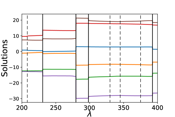
Figure 2: An age-path visualisation. Different vertical lines represent different types of critical points. The figure is plotted on random 60% features from diabetes dataset using Lasso with $\alpha=0.01$.

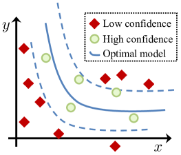
Figure 3: An example of set partition in 2-D space. Sample points of same colors belong to one set. The two dashed lines represent partition boundaries (smooth surfaces), which satisfies $l_{i}=\lambda$.

2 Preliminaries

2.1 Self-paced Learning

Suppose we have a dataset containing the label vector $\boldsymbol{y}\in\mathbb{R}^{n}$ and $X\in\mathbb{R}^{n\times d}$, where $n$ samples with $d$ features are included. The $i$-th row $X_{i}$ represents the $i$-th data sample $x_{i}$ (i.e., the $i$-th observation). In this paper, the following unconstrained learning problem is considered

$$\min_{\boldsymbol{w}\in\mathbb{R}^{d}}~{}\sum_{i=1}^{n}\ell\left(x_{i},y_{i};\boldsymbol{w}\right)+\sum_{j=1}^{m}\alpha_{j}\mathcal{R}_{j}(\boldsymbol{w}),$$ (1)

where $\mathcal{R}_{j}(\cdot)$ is the regularization item with a positive trade-off parameter $\alpha_{j}$, and $\ell_{i}(\boldsymbol{w})$ denotes loss function w.r.t. $\boldsymbol{w}$.

Definition 1 ($\mathbb{PC}^{r}$ Function).

Let $f:U\rightarrow\mathbb{R}$ be a continuous function on the open set $U\in\mathbb{R}^{n}$. If $\left\{f_{i}\right\}_{i\in I_{f}}$ is a set of $\mathbb{C}^{r}$ (i.e., r-times continuously differentiable) functions such that $f(\boldsymbol{x})\in\left\{f_{i}(\boldsymbol{x})\right\}_{i\in I_{f}}$ holds for every $\boldsymbol{x}\in U$, then $f$ is an r-times piecewise continuously differentiable function, namely $\mathbb{PC}^{r}$ function. The $\left\{f_{i}\right\}_{i\in I}$ is a set of selection functions of $f$.

Assumption 1.

We assume that $\ell_{i}(\boldsymbol{w})$ and $\mathcal{R}_{j}(\boldsymbol{w})$ are convex $\mathbb{PC}^{r}$ functions each with a set of selection functions $\bigcup_{k\in I_{\ell_{i}}}\left\{D_{\ell_{i}}^{k}\right\}$ and $\bigcup_{k\in I_{\mathcal{R}_{j}}}\left\{D_{\mathcal{R}_{j}}^{k}\right\}$, respectively.

In self-paced learning, the goal is to jointly train the model parameter $\boldsymbol{w}$ and the latent weight variable $\boldsymbol{v}$ by minimizing

$$\underset{\boldsymbol{w}\in\mathbb{R}^{d},\boldsymbol{v}\in[0,1]^{n}}{\operatorname{argmin}}\mathcal{L}(\boldsymbol{w},\boldsymbol{v}):=\sum_{j=1}^{m}\alpha_{j}\mathcal{R}_{j}(\boldsymbol{w})+\sum_{i=1}^{n}\left[v_{i}l_{i}\left(\boldsymbol{w}\right)+\rule{0.0pt}{10.0pt}f\left(v_{i},\lambda\right)\right],$$ (2)

where $f\left(v,\lambda\right)$ represents the SP-regularizer.

2.2 SP-regularizer

Definition 2 (SP-regularizer [35]).

Suppose that $v$ is a weight variable, $\ell$ is the loss, and $\lambda$ is the age parameter. $f(v,\lambda)$ is called a self-paced regularizer, if
(i)$f(v,\lambda)$ is convex with respect to $v\in[0,1]$;
(ii)$v^{*}(\ell,\lambda)$ is monotonically decreasing w.r.t. $\ell$, and holds $\lim_{\ell\rightarrow 0}v^{*}(\ell,\lambda)=1,\lim_{\ell\rightarrow\infty}v^{*}(\ell,\lambda)=0$;
(iii)$v^{*}(\ell,\lambda)$ is monotonically increasing w.r.t. $\lambda$, and holds $\lim_{\lambda\rightarrow\infty}v^{*}(\ell,\lambda)\leq 1,\lim_{\lambda\rightarrow 0}v^{*}(\ell,\lambda)=0$,

where $v^{*}(\ell,\lambda)=\arg\min_{v\in[0,1]}v\ell+f(v,\lambda)$.

The Definition 2 gives axiomatic definition of SP-regularizer. Some frequently utilized SP-regularizers include $f^{H}(v,\lambda)=-\lambda v$, $f^{L}(v,\lambda)=\lambda\left(\frac{1}{2}v^{2}-v\right)$, $f^{M}(v,\lambda,\gamma)=\frac{\gamma^{2}}{v+\gamma/\lambda}$ and $f^{LOG}(v,\lambda,\alpha)=\frac{1}{\alpha}KL(1+\alpha\lambda,v)$, which represents hard, linear, mixture, LOG SP-regularizer, respectively.

2.3 Biconvex Optimization

Definition 3 (Biconvex Function).

A function $f:B\rightarrow\mathbb{R}$ on a biconvex set $B\subseteq\mathcal{X}\times\mathcal{Y}$ is called a biconvex function on $B$, if $f_{x}(\cdot):=f(x,\cdot):B_{x}\rightarrow\mathbb{R}$ is a convex function on $B_{x}$ for every fixed $x\in\mathcal{X}$ and $f_{y}(\cdot):=f(\cdot,y):B_{y}\rightarrow\mathbb{R}$ is a convex function on $B_{y}$ for every fixed $y\in\mathcal{Y}$.

Definition 4 (Partial Optimum).

Let $f:B\rightarrow\mathbb{R}$ be a given biconvex function and let $\left(x^{*},y^{*}\right)\in B$. Then, $z^{*}=\left(x^{*},y^{*}\right)$ is called a partial optimum of $f$ on $B$, if $f\left(x^{*},y^{*}\right)\leq f\left(x,y^{*}\right)\forall x\in B_{y^{*}}\text{ and }f\left(x^{*},y^{*}\right)\leq f\left(x^{*},y\right)\forall y\in B_{x^{*}}.$

Algorithm 1  Alternate Convex Search (ACS)

0:  Dataset ${X}$ and $y$, age parameter $\lambda$.

1:  Initialize $\boldsymbol{w}$.

2:  while not converged  do

3:     Update $\boldsymbol{v}^{*}=\operatorname{argmin}_{\boldsymbol{v}}\mathcal{L}(\boldsymbol{w}^{*},\boldsymbol{v})$.

4:     Update $\boldsymbol{w}^{*}=\operatorname{argmin}_{\boldsymbol{w}}\mathcal{L}(\boldsymbol{w},\boldsymbol{v}^{*})$.

5:  end while

5:   $\hat{\boldsymbol{w}}$

Optimizing (2) leads to a biconvex optimization problem and is generally non-convex with fixed $\lambda$, in which a number of local minima exist and previous convex optimization tools can’t achieve a promising effect [36]. It’s reasonably believed that algorithms taking advantage of the biconvex structure are more efficient in the corresponding setting. For frequently used one, ACS (c.f. Algorithm 1) is presented to optimize $x$ and $y$ in $f(x,y)$ alternately until terminating condition is met.

Remark 1.

The order of the optimization subproblems in line 3 & 4 in Algorithm 1 can be permuted.

Theorem 1.

[37] Let $\mathcal{X}\subseteq\mathbb{R}^{n}$ and $\mathcal{Y}\subseteq\mathbb{R}^{m}$ be closed sets and let $f:\mathcal{X}\times\mathcal{Y}\rightarrow\mathbb{R}$ be continuous. Let the sequence $\left\{z_{i}\right\}_{i\in\mathbb{N}_{+}}$ generated by ACS converges to $z^{*}\in\mathcal{X}\times\mathcal{Y}$. Then $z^{*}$ is a partial optimum.

2.4 Theoretical Consistency

Researchers in earlier study [35] theoretically conducted the latent SPL loss (a.k.a., implicit objective) and further proved that the SPL paradigm converges to the stationary point of the latent objective under some mild assumptions, which gives explanation to the robustness of the SPL [35, 38]. In this paper, we focus on the partial optimum of original SPL objective and result is given in Theorem 2.

Theorem 2.

Under the same assumptions in Theorem 2 of [38], the partial optimum of SPL objective consists with the stationary point of implicit SPL objective $G_{\lambda}$.

Factoring in both Theorem 1 & 2, the ACS procedure (or its variations) used in SPL paradigm indeed finds the partial optimum of SPL objective, which unifies the two proposed analysis frameworks and provides more in-depth understanding to the intrinsic mechanism behind the SPL regime.

3 Age-Path Tracking

3.1 Objective Reformulation

For the convenience of derivation, we denote the set $I_{\mathcal{R}}$ or $\bar{I}_{\mathcal{R}}$ to be the set of indexes $j$ where $\mathcal{R}_{j}$ is differentiable or non-differentiable at $\boldsymbol{w}$, respectively. Similarly, we have $I_{\ell}$ and $\bar{I}_{\ell}$ w.r.t. $\ell_{i}$.

$$\footnotesize x_{i}\in~{}\begin{cases}\mathcal{E},&\text{ if }l_{i}<~{}\lambda~{}\text{(or $\left(\dfrac{\lambda\gamma}{\lambda+\gamma}\right)^{2}$ in mixture $f\left(v,\lambda\right)$)}\\ \mathcal{D},&\text{ if }l_{i}\geqslant~{}\lambda~{}\text{(or $\lambda^{2}$ in mixture $f\left(v,\lambda\right)$)}\\ \mathcal{M},&\text{ if }\left(\dfrac{\lambda\gamma}{\lambda+\gamma}\right)^{2}\leqslant l_{i}\leqslant\lambda^{2}~{}\text{(only used in mixture $f\left(v,\lambda\right)$)}\end{cases}$$

Moreover, the training of the SPL is essentially a process of adaptive sample selection, so we classify all the sample points in the training set into different sets $\mathcal{P}:=\left\{\mathcal{E},\mathcal{D},\mathcal{M},...\right\}$ according to their confidence (or loss). Figure 3 illustrates a partition example when hard, linear or LOG SP-regularizer is used. Since subproblem in line $3$ of Algorithm 1 always gives closed-form solutions in iterations, we can rewrite SPL optimization objective as (3), which is indeed equivalent to searching a partial optimum of (2).

$$\text{ Compute }\hat{\boldsymbol{w}}\text{,~{} s.t.~{}}\hat{\boldsymbol{w}}\in\arg\min_{\boldsymbol{w}\in\mathbb{R}^{d}}~{}\sum_{j=1}^{m}\alpha_{j}\mathcal{R}_{j}(\boldsymbol{w})+\sum_{J\in\mathcal{P}}\sum_{i\in J}v_{i}^{*}\left(l_{i}(\hat{\boldsymbol{w}}),\lambda\right)\cdot\ell_{i}(\boldsymbol{w}).$$ (3)

3.2 Piecewise Smooth Age-path

The KKT theorem [25] states that (3) holds iff

$$\mathbf{0}\in~{}\sum_{j=1}^{m}\alpha_{j}\partial\mathcal{R}_{j}(\hat{\boldsymbol{w}})+\sum_{J\in\mathcal{P}}\sum_{i\in J}v^{*}\left(l_{i}(\hat{\boldsymbol{w}}),\lambda\right)\cdot\partial\ell_{i}(\hat{\boldsymbol{w}}),$$ (4)

where $\partial(\cdot)$ denotes the subdifferential (set of all subgradients). In the $\mathbb{P}\mathbb{C}^{r}$ setting, subgradient can be expressed explicitly by essentially active functions (c.f. Lemma 1).

Definition 5 (Essentially Active Set).

Let $f:U\rightarrow\mathbb{R}$ be a $\mathbb{PC}^{r}$ function on the open set $U\in\mathbb{R}^{n}$ with a set of selection functions $\left\{f_{i}\right\}_{i\in I_{f}}$. For $\boldsymbol{x}\in U$, we call $I_{f}^{a}(\boldsymbol{x}):=\left\{i\in I_{f}:f(\boldsymbol{x})=f_{i}(\boldsymbol{x})\right\}$ is the active set at $\boldsymbol{x}$, and $I_{f}^{e}(\boldsymbol{x}):=\left\{i\in I_{f}:\boldsymbol{x}\in\operatorname{\bf cl}\left(\rule{0.0pt}{10.0pt}\operatorname{\bf int}\left(\rule{0.0pt}{9.0pt}\left\{\boldsymbol{y}\in U:~{}f(\boldsymbol{y})=f_{i}(\boldsymbol{y})\right\}\right)\right)\right\}$ is the essentially active set at $\boldsymbol{x}$, where cl$(\cdot)$ and int$(\cdot)$ denote the closure and interior of a set.

Lemma 1.

[39] Let $f:U\rightarrow\mathbb{R}$ be a $\mathbb{P}\mathbb{C}^{r}$ function on an open set $U$ and $\bigcup_{i\in I_{f}}\left\{f_{i}\right\}$ is a set of selection functions of $f$, then $\partial f(\boldsymbol{x})=\operatorname{conv}(\bigcup_{i\in I_{f}^{e}(\boldsymbol{x})}\left\{f_{i}(x)\right\})=\{\sum_{i\in I_{f}^{e}(\boldsymbol{x})}t_{i}\nabla f_{i}(\boldsymbol{x}):\sum_{i\in I_{f}^{e}(\boldsymbol{x})}t_{i}=1,~{}t_{i}\geq 0\}.$ Especially, if $f$ is differentiable at $\boldsymbol{x}$, $\partial f(\boldsymbol{x})=\{\nabla f(\boldsymbol{x})\}$.

Assumption 2.

We assume that $I_{\mathcal{R}_{j}}^{a}(\boldsymbol{x})=I_{\mathcal{R}_{j}}^{e}(\boldsymbol{x}),I_{\ell_{i}}^{a}(\boldsymbol{x})=I_{\ell_{i}}^{e}(\boldsymbol{x})$ holds for all $\boldsymbol{x}$ considered and all $\mathcal{R}_{j},\ell_{i}$ in the following.

We adopt a mild relaxation as shown in Assumption 2. Investigation [40] confirmed that it can be easily established in most practical scenarios. Without loss of generality, we suppose the following Assumption 3 also holds to further ease the notation burden.

Assumption 3.

We assume that $\mathcal{R}_{j},\ell_{i}$ are non-differentiable at $\boldsymbol{x}$ with multiple active selection functions, where $j\in\{1,\ldots,m\},~{}i\in\{1,\ldots,n\}.$

Therefore, the condition (4) can be rewritten in detail. Formally, there exists $\hat{\boldsymbol{t}}_{\mathcal{R}}$ and $\hat{\boldsymbol{t}}_{\ell}$ such that

$$\sum_{j=1}^{m}\sum_{k\in I_{\mathcal{R}_{j}}^{a}(\hat{\boldsymbol{w}})}\alpha_{j}\hat{t}_{\mathcal{R}_{j}}^{k}(\hat{\boldsymbol{w}})\nabla D_{\mathcal{R}_{j}}^{k}(\hat{\boldsymbol{w}}) +\sum_{J\in\mathcal{P}}\sum_{i\in J}\sum_{k\in I_{\ell_{i}}^{a}(\hat{\boldsymbol{w}})}v^{*}_{i}\left(\ell_{i}(\hat{\boldsymbol{w}}),\lambda\right)\hat{t}_{\ell_{i}}^{k}(\hat{\boldsymbol{w}})\nabla D_{\ell_{i}}^{k}(\hat{\boldsymbol{w}})=\boldsymbol{0},$$ (5)

$$D_{\mathcal{R}_{j}}^{k}(\hat{\boldsymbol{w}})-D_{\mathcal{R}_{j}}^{r_{j}}(\hat{\boldsymbol{w}}) =0,\quad\forall k\in I_{\mathcal{R}_{j}}^{a}(\hat{\boldsymbol{w}})\backslash\{r_{j}\},\quad\forall j\in\bar{I}_{\mathcal{R}}$$

$$D_{\ell_{i}}^{k}(\hat{\boldsymbol{w}})-D_{\ell_{i}}^{l_{i}}(\hat{\boldsymbol{w}}) =0,\quad\forall k\in I_{\ell_{i}}^{a}(\hat{\boldsymbol{w}})\backslash\{l_{i}\},\quad\forall i\in\bar{I}_{\ell}$$

$$\quad\sum_{k\in I_{\mathcal{R}_{j}}^{a}(\hat{\boldsymbol{w}})}\hat{t}_{\mathcal{R}_{j}}^{k}(\hat{\boldsymbol{w}})-1 =0,\quad\hat{t}_{\mathcal{R}_{j}}^{k}(\hat{\boldsymbol{w}})\geq 0,\quad 1\leq j\leq m$$

$$\sum_{k\in I_{\ell_{i}}^{a}(\hat{\boldsymbol{w}})}\hat{t}_{\ell_{i}}^{k}(\hat{\boldsymbol{w}})-1 =0,\quad\hat{t}_{\ell_{i}}^{k}(\hat{\boldsymbol{w}})\geq 0,\quad 1\leq i\leq n,$$

where $r_{j},l_{i}$ is randomly selected from $I_{\mathcal{R}_{j}}^{a},I_{\ell_{i}}^{a}$ and being fixed. The second and third equations in (5) describe the active sets while the last two equations describe the subgradients. When the partial optimum is on the smooth part, we denote the left side of equations (5) to be a $\mathbb{C}^{1}$ function $\mathcal{F}$, thus revealing that the solution path lies on the smooth manifold $\mathcal{F}\left(\boldsymbol{w},\lambda,\boldsymbol{t}_{\mathcal{R}},\boldsymbol{t}_{\ell}\right)=\mathbf{0}$. By the time it comes across the kink, we need to refresh the index partitions and update (5) to run next segment of path. WLOG, we postulate that the initial point is non-degenerate (i.e., the $\boldsymbol{J}_{\boldsymbol{w},\boldsymbol{t}_{\mathcal{R}},\boldsymbol{t}_{\ell}}$ is invertible). By directly applying the implicit function theorem, the existence and uniqueness of a local $\mathbb{C}^{1}$ solution path $\left(\hat{\boldsymbol{w}},\hat{\boldsymbol{t}}_{\mathcal{R}},\hat{\boldsymbol{t}}_{\mathcal{\ell}}\right)$ can be established over here. Drawing from the theory of differential geometry gives another intuitive understanding of age-path, which tells that the first equation in (5) indeed uses an analogue moving frame [41] to represent a smooth curve that consists of the smooth structure.

Theorem 3.

Given a partial optimum $\left(\hat{\boldsymbol{w}},\boldsymbol{v}^{*}\left(\hat{\boldsymbol{w}},\lambda\right)\right)$ at $\lambda_{0}$, $\hat{\boldsymbol{t}}_{\mathcal{R}},\hat{\boldsymbol{t}}_{\ell}$ in (5) can be solved from $\mathcal{F}\left(\hat{\boldsymbol{w}},\lambda_{0},\hat{\boldsymbol{t}}_{\mathcal{R}},\hat{\boldsymbol{t}}_{\ell}\right)=\mathbf{0}$. If the Jacobian $\boldsymbol{J}_{\boldsymbol{w},\boldsymbol{t}_{\mathcal{R}},\boldsymbol{t}_{\ell}}$ is invertible at $\left(\hat{\boldsymbol{w}},\hat{\boldsymbol{t}}_{\mathcal{R}},\hat{\boldsymbol{t}}_{\ell}\right)$, then in an open neighborhood of $\lambda_{0}$, $\left(\hat{\boldsymbol{w}},\hat{\boldsymbol{t}}_{\mathcal{R}},\hat{\boldsymbol{t}}_{\ell}\right)$ is a $\mathbb{C}^{1}$ function w.r.t. $\lambda$ and fits the ODEs

$$\frac{d\left(\begin{array}[]{c}\hat{\boldsymbol{w}}\\ \hat{\boldsymbol{t}_{\mathcal{R}}}\\ \hat{\boldsymbol{t}_{\ell}}\end{array}\right)}{\rule{0.0pt}{10.0pt}d\lambda}=-\boldsymbol{J}_{\boldsymbol{w},\boldsymbol{t}_{\mathcal{R}},\boldsymbol{t}_{\ell}}^{-1}\cdot\boldsymbol{J}_{\lambda},$$ (6)

in which the explicit expressions of $\boldsymbol{J}_{\boldsymbol{w},\boldsymbol{t}_{\mathcal{R}},\boldsymbol{t}_{\ell}}^{-1},\boldsymbol{J}_{\lambda}$ are listed in Appendix A.

Corollary 1.

If all the functions are smooth in a neighborhood of the initial point, then (6) can be simplified as $d\hat{\boldsymbol{w}}/d\lambda=-\boldsymbol{J}_{\boldsymbol{w}}^{-1}\cdot\boldsymbol{J}_{\lambda}.$

Remark 2.

Our supplement parts in Appendix A present additional discussions.

3.3 Critical Points

By solving the initial value problem (6) numerically with ODE solvers, the solution path regarding to $\lambda$ can be computed swiftly before any of $\mathcal{P},I_{\mathcal{R}}$ or $I_{\ell}$ changes. We denote such point where the set changes a critical point, which can be divided into turning point or jump point on the basis of path’s property at that point. To be more specific, the age-path is discontinuous at a jump point, while being continuous but non-differentiable at the turning point. This is also verified by Figure 2 and large quantity of numerical experiments. At turning points, the operation of the algorithm is to update $\mathcal{P},I_{\mathcal{R}},I_{\ell}$ according to index violator(s) and move on to the next segment. At jump points, path is no longer continuous and warm-start can be utilized to speed up the training procedure. The total number of critical points on the solution path is estimated at approximately $\mathcal{O}(|\mathcal{D}\cup\mathcal{M}|)$. Consequently, we present a heuristic trick to figure out the type of a critical point with complexity $\mathcal{O}(d)$, so as to avoid excessive restarts. As a matter of fact, the solutions returned by the numerical ODE solver is continuous with the fixed set, despite it may actually passes a jump point. In this circumstance, the solutions returned by ODEs have deviated from the ground truth partial optimum. Hence it’s convenient that we can detect KKT conditions to monitor this behavior. This approach enjoys higher efficiency than detecting the partition conditions themselves, especially when the set partition is extraordinarily complex.

3.4 GAGA Algorithm

Algorithm 2  Generalized Age-path Algorithm (GAGA)

Input: Initial solution $\hat{\boldsymbol{w}}|_{\lambda_{t}=\lambda_{min}}$, $X$, $y$, $\lambda_{min}$ and $\lambda_{max}$.
Output: Age-Path $\hat{\boldsymbol{w}}\left(\lambda\right)$ on $\left[\lambda_{min},\lambda_{max}\right]$.

1:  $\lambda_{t}\leftarrow\lambda_{min}$, set $\mathcal{P},I_{\mathcal{R}},I_{\ell}$ according to $\hat{\boldsymbol{w}}|_{\lambda_{t}}$.

2:  while $\lambda_{t}\leq\lambda_{max}$  do

3:     Solve (6) and examine partition $\mathcal{P},I_{\mathcal{R}},I_{\ell}$ simultaneously.

4:     if Partition $\mathcal{P},I_{\mathcal{R}},I_{\ell}$ was not met then

5:        Update $\mathcal{P},I_{\mathcal{R}},I_{\ell}$ according to index violator(s).

6:        Solve (6) with updated $\mathcal{P},I_{\mathcal{R}},I_{\ell}$.

7:        if KKT conditions are not met then

8:           Warm start at $\lambda_{t}+\delta$ (for a small $\delta>0$).

9:        end if

10:     end if

11:  end while

There has been extensive research in applied mathematics on numerical methods for solving ODEs, where the solver could automatically determine the step size of $\lambda$ when solving (6). In the tracking process, we compute the solutions with regard to $\lambda$. After detecting a new critical point, we need to reset $\mathcal{P},I_{\mathcal{R}},I_{\ell}$ at turning point while warm-start is required for jump point. The above procedure is repeated until we traverse the entire interval $\left[\lambda_{min},\lambda_{max}\right]$. We show the detailed procedure in Algorithm 2. The main computational burden occurs in solving $\boldsymbol{J}^{-1}$ in (6) with an approximate complexity $\mathcal{O}(p^{3})$ in general, where $p$ denotes the dimension of $\boldsymbol{J}$. Further promotion can be made via decomposition or utilizing the sparse representation of $\boldsymbol{J}$ on specific learning problems.

4 Practical Guides

In this section, we provide practical guides of using the GAGA to solve two important learning problems, i.e., classic SVM and Lasso. The detailed steps of algorithms are displayed in Appendix C.

4.1 Support Vector Machines

Support vector machine (SVM) [33] has attracted much attention from researchers in the areas of bioinformatics, computer vision and pattern recognition. Given the dataset $X$ and label $\boldsymbol{y}$, we focus on the classic support vector classification as

$$\min_{\boldsymbol{w},b}\frac{1}{2}\|\boldsymbol{w}\|_{\mathcal{H}}^{2}+\sum_{i=1}^{n}C\max\left\{0,~{}1-y_{i}(\langle\phi(x_{i}),\boldsymbol{w}\rangle+b)\right\},$$ (7)

where $\mathcal{H}$ is the reproducing kernel Hilbert space (RKHS) with the inner product $\langle\cdot\rangle$ and corresponding kernel function $\phi$. Seeing that (5) still holds in infinite dimensional $\mathcal{H}$, the above analyses can be directly applied here. We also utilize the kernel trick [42] to avoid involving the explicit expression of $\phi$. In consistent with the framework, we have $~{}\ell_{i}=C\max\left\{0,g_{i}\right\}$ and $g_{i}=1-y_{i}(\langle\phi(x_{i}),\boldsymbol{w}\rangle+b).$ The $I_{\ell}$ and $\mathcal{P}$ are determined by $\boldsymbol{g}$, thus we merely need to refine the division of $\mathcal{E}$ as $\mathcal{E}_{N}=\{i\in\mathcal{E}:g_{i}<0\},\mathcal{E}_{Z}=\{i\in\mathcal{E}:g_{i}=0\}$ and $\mathcal{E}_{P}=\{i\in\mathcal{E}:g_{i}>0\}$, which gives $I_{\ell}=\mathcal{E}_{N}\cup\mathcal{E}_{P}\cup\mathcal{D}(\cup\mathcal{M})$. Afterwards, with some simplifications and denoting $\hat{\boldsymbol{\alpha}}=C\boldsymbol{v}^{*}\odot\hat{\boldsymbol{t}},$ we can obtain a simplified version of (5), from where the age-path can be equivalently calculated w.r.t. optimal $(\hat{\boldsymbol{\alpha}},\hat{b})$.

Proposition 1.

When $\boldsymbol{\alpha},b$ indicate a partial optimum, the dynamics of optimal $\boldsymbol{\alpha},b$ in (7) w.r.t. $\lambda$ for the linear and mixture SP-regularizer are shown as

$$\frac{d\left(\begin{array}[]{c}\boldsymbol{\alpha}_{\mathcal{E}_{Z}}\\ \boldsymbol{\alpha}_{\mathcal{E}_{P}}\\ b\end{array}\right)}{\rule{0.0pt}{10.0pt}d\lambda}=\left(\begin{array}[]{ccc}-\boldsymbol{y}_{\mathcal{E}_{Z}}^{T}&-\boldsymbol{y}_{\mathcal{E}_{P}}^{T}&0\\ Q_{\mathcal{E}_{Z}\mathcal{E}_{Z}}&Q_{\mathcal{E}_{Z}\mathcal{E}_{P}}&\boldsymbol{y}_{\mathcal{E}_{Z}}\\ \frac{C^{2}}{\lambda}Q_{\mathcal{E}_{P}\mathcal{E}_{Z}}&\frac{C^{2}}{\lambda}Q_{\mathcal{E}_{P}\mathcal{E}_{P}}-I_{\mathcal{E}_{P}\mathcal{E}_{P}}&\frac{C^{2}}{\lambda}\boldsymbol{y}_{\mathcal{E}_{P}}\par\end{array}\right)^{-1}\left(\begin{array}[]{c}0\\ \boldsymbol{0}_{\mathcal{E}_{Z}}\\ -\frac{C}{\lambda^{2}}\boldsymbol{\ell}_{\mathcal{E}_{P}}\par\end{array}\right),$$ (8)

$$\frac{d\left(\begin{array}[]{c}\boldsymbol{\alpha}_{\mathcal{E}_{Z}}\\ \boldsymbol{\alpha}_{\mathcal{M}}\\ b\end{array}\right)}{\rule{0.0pt}{10.0pt}d\lambda}=\left(\begin{array}[]{ccc}-\boldsymbol{y}_{\mathcal{E}_{Z}}^{T}&-\boldsymbol{y}_{\mathcal{M}}^{T}&0\\ Q_{\mathcal{E}_{Z}\mathcal{E}_{Z}}&Q_{\mathcal{E}_{Z}\mathcal{M}}&\boldsymbol{y}_{\mathcal{E}_{Z}}\\ \frac{C^{2}\gamma}{2}\tilde{Q}_{\mathcal{M}\mathcal{E}_{Z}}&\frac{C^{2}\gamma}{2}\tilde{Q}_{\mathcal{M}\mathcal{M}}-I_{\mathcal{M}\mathcal{M}}&\frac{C^{2}\gamma}{2}\tilde{\boldsymbol{y}}_{\mathcal{M}}\par\end{array}\right)^{-1}\left(\begin{array}[]{c}0\\ \boldsymbol{0}_{\mathcal{E}_{Z}}\\ -\frac{C\gamma}{\lambda^{2}}\boldsymbol{1}_{\mathcal{M}}\par\end{array}\right),$$ (9)

respectively, where $\tilde{Q}_{\mathcal{M}\mathcal{E}_{Z}}=Diag\{\boldsymbol{\ell}_{\mathcal{M}}^{-\frac{3}{2}}\}Q_{\mathcal{M}\mathcal{E}_{Z}},\tilde{Q}_{\mathcal{M}\mathcal{M}}=Diag\{\boldsymbol{\ell}_{\mathcal{M}}^{-\frac{3}{2}}\}Q_{\mathcal{M}\mathcal{M}},\tilde{\boldsymbol{y}}_{\mathcal{M}}=\boldsymbol{\ell}_{\mathcal{M}}^{-\frac{3}{2}}\odot\boldsymbol{y}_{\mathcal{M}}.$

Other components are constant as $\boldsymbol{\alpha}_{\mathcal{E}_{N}}=\boldsymbol{0}_{\mathcal{E}_{N}},\boldsymbol{\alpha}_{\mathcal{D}}=\boldsymbol{0}_{\mathcal{D}}$. Only for mixture regularizer, $\boldsymbol{\alpha}_{\mathcal{E}_{P}}=\boldsymbol{1}_{\mathcal{E}_{P}}$.

Critical Point. We track $\boldsymbol{g}$ along the path. The critical point is sparked off by any set in $\mathcal{E}_{N},\mathcal{E}_{Z},\mathcal{E}_{P},\mathcal{D}(,\mathcal{M})$ changes.

4.2 Lasso

Lasso [34] uses a sparsity based regularization term that can produce sparse solutions.

Given the dataset $X$ and label $\boldsymbol{y}$, the Lasso regression is stated as

$$\underset{\boldsymbol{w}\in\mathbb{R}^{d}}{\operatorname{min}}~{}\frac{1}{2n}\|X\boldsymbol{w}-\boldsymbol{y}\|^{2}+\alpha\left\|\boldsymbol{w}\right\|_{1}.$$ (10)

We expand $\|\boldsymbol{w}\|_{1}=\sum_{j=1}^{d}|w_{j}|$ and treat $|w_{j}|$ as $\mathcal{R}_{j}$ in (5), hence the $I_{\mathcal{R}}=\{1\leq j\leq d:w_{j}\neq 0\}$. We denote the set of active or inactive functions (components) by $\mathcal{A}=I_{\mathcal{R}},\bar{\mathcal{A}}=\bar{I}_{\mathcal{R}}$, respectively. In view of the fact that $\partial{|w_{j}|}$ removes $\boldsymbol{t}_{\mathcal{R}_{j}}$ from the equations in (5) for $j\in\bar{\mathcal{A}}$, we only pay attention to the $\mathcal{A}$ part w.r.t. the $(\boldsymbol{w}_{\mathcal{A}},\lambda)$. The $\boldsymbol{\ell}$ is defined as $\frac{1}{2n}{(}X\boldsymbol{w}-\boldsymbol{y}{)}^{2}$ in the following.

Proposition 2.

When $(\boldsymbol{w},\boldsymbol{v}^{*}(\boldsymbol{w},\lambda))$ is a partial optimum, the dynamics of optimal $\boldsymbol{w}$ in (10) w.r.t. $\lambda$ for the linear and mixture SP-regularizer are described as

$$\frac{d\boldsymbol{w}_{\mathcal{A}}}{d\lambda}=-\frac{\sqrt{2n}}{\lambda^{2}}\left(X_{\mathcal{A}\mathcal{E}}^{T}Diag\left\{\boldsymbol{1}_{\mathcal{E}}-\frac{3}{\lambda}\boldsymbol{\boldsymbol{\ell}}_{\mathcal{E}}\right\}X_{\mathcal{E}\mathcal{A}}\right)^{-1}X_{\mathcal{A}\mathcal{E}}^{T}\boldsymbol{\ell}_{\mathcal{E}}^{\frac{3}{2}},$$ (11)

$$\frac{d\boldsymbol{w}_{\mathcal{A}}}{d\lambda}=-\frac{\sqrt{2n}\gamma}{\lambda^{2}}\left(X_{\mathcal{A}\mathcal{E}\cup\mathcal{M}}^{T}\tilde{X}_{\mathcal{E}\cup\mathcal{M}\mathcal{A}}\right)^{-1}X_{\mathcal{A}\mathcal{E}\cup\mathcal{M}}^{T}\left(\begin{array}[]{c}\boldsymbol{0}_{\mathcal{E}}\\ \boldsymbol{\ell}_{\mathcal{M}}\end{array}\right),$$ (12)

respectively, where $\tilde{X}_{\mathcal{E}\cup\mathcal{M}\mathcal{A}}=\left(\begin{array}[]{c}X_{\mathcal{E}\mathcal{A}}\\ -\frac{\gamma}{\lambda}X_{\mathcal{M}\mathcal{A}}\end{array}\right)$ and $\boldsymbol{w}_{\bar{\mathcal{A}}}=\boldsymbol{0}_{\bar{\mathcal{A}}}.$

Critical Point. The critical point is encountered when $\mathcal{A}$ or $\mathcal{P}$ changes.

5 Experimental Evaluation

Dataset	Source	Samples	Dimensions	Task
mfeat-pixel	UCI [43]	2000	240	C
pendigits	UCI	3498	16
hiva agnostic	OpenML	4230	1620
music	OpenML [44]	1060	117	R
cadata	UCI	20640	8
delta elevators	OpenML	9517	8
houses	OpenML	22600	8
ailerons	OpenML	13750	41
elevator	OpenML	16600	18

Table 1: Datasets description in our experiments. The C=Classification, R=Regression.

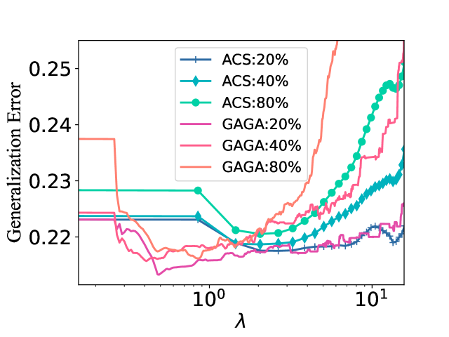
Figure 4: Robustness to noise. This figure shows the learning curve under different noise ratios, which confirms that the GAGA is more robust when in the setting of relatively high noise.

We present the empirical results of the proposed GAGA on two tasks: SVM for binary classification and Lasso for robust regression in the noisy environment. The results demonstrate that our approach outperforms existing SPL implementations on both tasks.

Dataset	Parameter			Competing Methods			Ours	Restarting times
	$C,\gamma_{\kappa}$	$\alpha$		Original	ACS	MOSPL	GAGA
mfeat-pixel†	1.00, 0.50	–		0.959$\pm 0.037$	0.976$\pm 0.015$	0.978$\pm 0.021$	0.986$\pm 0.016$	23
mfeat-pixel‡	1.00, 0.50	–		0.945$\pm 0.025$	0.947$\pm 0.031$	0.960$\pm 0.027$	0.983$\pm 0.013$	25
hiva agnostic†	1.00, 0.50	–		0.868$\pm 0.027$	0.941$\pm 0.009$	0.946$\pm 0.0137$	0.960$\pm 0.004$	8
pendigits†	1.00, 1.00	–		0.924$\pm 0.069$	0.960$\pm 0.005$	0.962$\pm 0.048$	0.971$\pm 0.046$	10
pendigits‡	1.00, 0.20	–		0.931$\pm 0.045$	0.942$\pm 0.089$	0.940$\pm 0.088$	0.944$\pm 0.089$	8
elevator†	–	2e-3		0.146$\pm 0.011$	0.144$\pm 0.012$	0.144$\pm 0.020$	0.143$\pm 0.012$	3
ailerons†	–	6e-3		0.674$\pm 0.071$	0.492$\pm 0.006$	0.491$\pm 0.041$	0.489$\pm 0.009$	16
music†	–	5e-3		0.325$\pm 0.009$	0.219$\pm 0.018$	0.215$\pm 0.012$	0.206$\pm 0.013$	123
delta elevators†	–	5e-3		0.783$\pm 0.153$	0.724$\pm 0.138$	0.679$\pm 0.057$	0.634$\pm 0.184$	4
houses†	–	5e-3		0.213$\pm 0.013$	0.209$\pm 0.010$	0.205$\pm 0.231$	0.201$\pm 0.146$	4

Table 2: Average results with the standard deviation in 20 runs on different datasets using the linear SP-regularizer. The top results in each row are in boldface.

Dataset	Parameter				Competing Methods			Ours	Restarting times
	$\gamma$	$C$,$\gamma_{\kappa}$	$\alpha$		Original	ACS	MOSPL	GAGA
mfeat-pixel†	0.20	1.00, 1.00	–		0.959$\pm 0.037$	0.963$\pm 0.038$	0.968$\pm 0.037$	0.973$\pm 0.040$	12
mfeat-pixel‡	0.50	0.20, 1.00	–		0.945$\pm 0.025$	0.962$\pm 0.024$	0.970$\pm 0.027$	0.977$\pm 0.015$	10
hiva agnostic†	0.50	1.00, 1.00	–		0.868$\pm 0.027$	0.946$\pm 0.004$	0.949$\pm 0.019$	0.957$\pm 0.007$	10
pendigits†	0.50	2.00, 1.00	–		0.924$\pm 0.069$	0.956$\pm 0.062$	0.957$\pm 0.071$	0.962$\pm 0.083$	32
pendigits‡	0.20	1.00, 1.00	–		0.931$\pm 0.045$	0.940$\pm 0.088$	0.942$\pm 0.089$	0.944$\pm 0.088$	30
cadata†	1.00	–,–	5e-3		0.798$\pm 0.039$	0.782$\pm 0.042$	0.754$\pm 0.084$	0.748$\pm 0.010$	13
ailerons†	0.50	–,–	5e-3		0.674$\pm 0.071$	0.452$\pm 0.057$	0.433$\pm 0.083$	0.422$\pm 0.090$	14
music†	0.50	–,–	6e-3		0.325$\pm 0.009$	0.218$\pm 0.009$	0.216$\pm 0.021$	0.213$\pm 0.027$	110
delta elevators†	0.50	–,–	5e-3		0.783$\pm 0.153$	0.663$\pm 0.074$	0.650$\pm 0.029$	0.595$\pm 0.132$	12
houses†	0.50	–,–	5e-3		0.213$\pm 0.013$	0.146$\pm 0.012$	0.144$\pm 0.027$	0.142$\pm 0.012$	8

Table 3: Average results with the standard deviation in 20 runs on different datasets using the mixture SP-regularizer. The top results in each row are in boldface.

Figure 5: The study of efficiency comparison. $y$-axis denotes the average running time (in seconds) with 20 runs. The interval $[\lambda_{min},\lambda_{max}]$ refers to the predefined searching area.

Baselines.

GAGA is compared against three baseline methods: 1) Original learning model without SPL regime. 2) ACS [20] performs sequential search of $\lambda$, which is the most commonly used algorithm in SPL implementations. 3) MOSPL [29] is a state-of-the-art age-path approach that using the multi objective optimization, in which the solution is derived with the age parameter $\lambda$ implicitly.

Datasets.

The Table 1 summarizes the datasets information. As universally known that SPL enjoys robustness in noisy environments, we impose 30% of noises into the real-world datasets. In particular, we generate noises by turning normal samples into poisoning ones by flipping their labels [45, 46] for classification tasks. For regression problem, noises are generated by the similar distribution of the training data as performed in [47].

Experiment Setting.

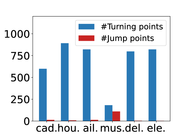
Figure 6: Histogram illustrating the number of different types of critical points. Names of datasets are shortened into the first 3 letters.

In experiments, we first verify the performance of GAGA and traditional ACS algorithm under different noise intensity to reflect the robustness of GAGA. We further study the generalization performance of GAGA with competing methods, so as to show its ability to select optimal model during the learning process. Meanwhile, we also evaluate the running efficiency between GAGA and existing SPL implementations in different settings, which examines the speedup of GAGA as well as its practicability. Finally, we count the number of restarts and different types of critical points when using GAGA, to investigate its ability to address critical points. For SVM, we use the Gaussian kernel $K(x_{1},x_{2})=\operatorname{exp}(-\gamma_{\kappa}\|x_{1}-x_{2}\|^{2})$. More details can be found in Appendix D.

Results.

Figure 4 illustrates that conventional ACS fails to reduce the generalization error due to heavy noises fed to the model at a large age (i.e., overfits the dataset), while GAGA makes up for this shortcoming by selecting the optimal model that merely learns the trust-worthy samples during the continuous learning process. Table 2 and 3 demonstrate an overall performance enhancing in GAGA than competing algorithms. The ‘†’ in tables denotes 30% of artificial noise, while ‘‡’ represents 20%. Note that performances are measured by accuracy and generalization error for classification and regression, respectively. The results guarantee that GAGA outperforms the state-of-the-art approaches in SPL under different circumstances. Figure 5 shows that GAGA also enjoys a high computational efficiency by changing the sample size as well as the predefined age sequence, emphasizing the potentials of utilizing GAGA in practice. The number of different types of critical points on some datasets is given in Figure 6. Corresponding restarting times can be found in Table 2 and 3, hence indicate that GAGA is capable of identifying different types of critical points and uses the heuristic trick to avoids restarts at massive turning points.

Additional Experiments in Appendix D.

We further demonstrate the ability of GAGA to address the relatively large sample size and present more histograms. In addition, we apply GAGA to the logistic regression [33] for classification. We also verify that conventional ACS indeed tracks an approximation path of partial optimum in experiments, which provides a more in-depth understanding towards SPL and the performance promotion brought by GAGA. We also conduct a comparative study to the state-of-the-art robust model for SVMs [48, 49, 50] and Lasso [51] besides the SPL domain.

6 Conclusion

In this paper, we connect the SPL paradigm to the partial optimum for the first time. Using this idea, we propose the first exact age-path algorithm able to tackle general SP-regularizer, namely GAGA. Experimental results demonstrate GAGA outperforms traditional SPL paradigm and the state-of-the-art age-path approach in many aspects, especially in the highly noisy environment. We further build the relationship between our framework and existing theoretical analyses on SPL regime, which provides more in-depth understanding towards the principle behind SPL.

Checklist

1. For all authors…

   1. Do the main claims made in the abstract and introduction accurately reflect the paper’s contributions and scope? [Yes]

   2. Did you describe the limitations of your work? [Yes] See Appendix E.

   3. Did you discuss any potential negative societal impacts of your work? [N/A]

   4. Have you read the ethics review guidelines and ensured that your paper conforms to them? [Yes]

2. If you are including theoretical results…

   1. Did you state the full set of assumptions of all theoretical results? [Yes]

   2. Did you include complete proofs of all theoretical results? [Yes]

3. If you ran experiments…

   1. Did you include the code, data, and instructions needed to reproduce the main experimental results (either in the supplemental material or as a URL)? [Yes]

   2. Did you specify all the training details (e.g., data splits, hyperparameters, how they were chosen)? [Yes]

   3. Did you report error bars (e.g., with respect to the random seed after running experiments multiple times)? [Yes]

   4. Did you include the total amount of compute and the type of resources used (e.g., type of GPUs, internal cluster, or cloud provider)? [Yes] See Appendix D.2.

4. If you are using existing assets (e.g., code, data, models) or curating/releasing new assets…

   1. If your work uses existing assets, did you cite the creators? [Yes] See Table 1.

   2. Did you mention the license of the assets? [Yes] Licenses are available referring to the provided links.

   3. Did you include any new assets either in the supplemental material or as a URL? [Yes]

   4. Did you discuss whether and how consent was obtained from people whose data you’re using/curating? [N/A]

   5. Did you discuss whether the data you are using/curating contains personally identifiable information or offensive content? [N/A]

5. If you used crowdsourcing or conducted research with human subjects…

   1. Did you include the full text of instructions given to participants and screenshots, if applicable? [N/A] This paper does not use crowdsourcing.

   2. Did you describe any potential participant risks, with links to Institutional Review Board (IRB) approvals, if applicable? [N/A] This paper does not use crowdsourcing.

   3. Did you include the estimated hourly wage paid to participants and the total amount spent on participant compensation? [N/A] This paper does not use crowdsourcing.

Appendix

Appendix A Supplementary Notes for Section 3

In this section, we present some additional discussions and theoretical results for Section 3.

A.1 Explicit Expression

The goal of this section is to obtain precise and explicit expressions of the Jacobian matrices in (6).

Firstly, the $\boldsymbol{J}_{\boldsymbol{w},\boldsymbol{t}_{\mathcal{R}},\boldsymbol{t}_{\ell}}^{-1}$ has the form of

$$\boldsymbol{J}_{\boldsymbol{w},\boldsymbol{t}_{\mathcal{R}},\boldsymbol{t}_{\ell}}^{-1}=\left(\begin{array}[]{cc}\tilde{\boldsymbol{F}}_{\boldsymbol{w}}&\tilde{\boldsymbol{F}}_{\boldsymbol{t}}\\ \left(\begin{array}[]{c}\tilde{\boldsymbol{D}}\\ \boldsymbol{O}\end{array}\right)&\left(\begin{array}[]{c}\boldsymbol{O}\\ \tilde{\boldsymbol{I}}\end{array}\right)\end{array}\right)^{-1},$$ (13)

in which

$$\tilde{\boldsymbol{F}}_{\boldsymbol{w}}=\sum_{j=1}^{m}\sum_{k\in I_{\mathcal{R}_{j}}^{a}(\hat{\boldsymbol{w}})}\alpha_{j}\hat{t}_{\mathcal{R}_{j}}^{k}(\hat{\boldsymbol{w}})\nabla^{2}D_{\mathcal{R}_{j}}^{k}(\hat{\boldsymbol{w}})+\sum_{J\in\mathcal{P}}\sum_{i\in J}\sum_{k\in I_{\ell_{i}}^{a}(\hat{\boldsymbol{w}})}v^{*}_{i}\left(\ell_{i}(\hat{\boldsymbol{w}}),\lambda\right)\hat{t}_{\ell_{i}}^{k}(\hat{\boldsymbol{w}})\nabla^{2}D_{\ell_{i}}^{k}(\hat{\boldsymbol{w}}),$$

$$\tilde{\boldsymbol{F}}_{\boldsymbol{t}}=\left(\begin{array}[]{cc}\mathbin{+\mkern-10.0mu+}_{1\leq j\leq m,k\in I_{\mathcal{R}_{j}}^{a}}\nabla D_{\mathcal{R}_{j}}^{k}(\hat{\boldsymbol{w}})&\mathbin{+\mkern-10.0mu+}_{\mathcal{J}\in\mathcal{P},j\in\mathcal{J},k\in I_{\ell_{i}}^{a}}\alpha_{j}\nabla D_{\ell_{j}}^{k}(\hat{\boldsymbol{w}})\end{array}\right),$$

$$\tilde{\boldsymbol{D}}=\left(\begin{array}[]{c}\left(\mathbin{+\mkern-10.0mu+}_{1\leq j\leq m,k\in I_{\mathcal{R}_{j}}^{a}\backslash\{r_{j}\}}\nabla D_{\mathcal{R}_{j}}^{k}(\hat{\boldsymbol{w}})-\nabla D_{\mathcal{R}_{j}}^{r_{j}}(\hat{\boldsymbol{w}})\right)^{T}\\ \left(\mathbin{+\mkern-10.0mu+}_{\mathcal{J}\in\mathcal{P},j\in\mathcal{J},k\in I_{\ell_{i}}^{a}\backslash\{l_{i}\}}\nabla D_{\ell_{i}}^{k}(\hat{\boldsymbol{w}})-\nabla D_{\ell_{i}}^{l_{i}}(\hat{\boldsymbol{w}})\right)^{T}\end{array}\right),$$

$$\tilde{\boldsymbol{I}}=\left(\begin{array}[]{c}\left(\mathbin{+\mkern-10.0mu+}_{i=1}^{n}\left(\begin{array}[]{c}\boldsymbol{1}_{I_{\mathcal{R}_{j}}^{a}}\\ \boldsymbol{0}_{\bar{I}_{\mathcal{R}_{j}}^{a}}\end{array}\right)\right)^{T}\\ \left(\mathbin{+\mkern-10.0mu+}_{\mathcal{J}\in\mathcal{P},j\in\mathcal{J}}\left(\begin{array}[]{c}\boldsymbol{1}_{I_{\ell_{i}}^{a}}\\ \boldsymbol{0}_{\bar{I}_{\ell_{i}}^{a}}\end{array}\right)\right)^{T}\end{array}\right).$$

The symbol $\mathbin{+\mkern-10.0mu+}$ denotes column matrix concatenation, following the convention in Haskell Language.

Similarly, $\boldsymbol{J}_{\lambda}$ is given by

$$\boldsymbol{J}_{\lambda}=\left(\begin{array}[]{c}\tilde{\boldsymbol{F}}_{\lambda}\\ \boldsymbol{0}\end{array}\right),$$ (14)

where

$$\tilde{\boldsymbol{F}}_{\lambda}=\sum_{J\in\mathcal{P}}\sum_{i\in J}\sum_{k\in I_{\ell_{i}}^{a}(\hat{\boldsymbol{w}})}\dfrac{\partial v^{*}_{i}\left(\ell_{i}(\hat{\boldsymbol{w}}),\lambda\right)}{\partial\lambda}\hat{t}_{\ell_{i}}^{k}(\hat{\boldsymbol{w}})\nabla D_{\ell_{i}}^{k}(\hat{\boldsymbol{w}}).$$

As an outcome, (6) can be explicitly expressed via

$$\frac{d\left(\begin{array}[]{c}\hat{\boldsymbol{w}}\\ \hat{\boldsymbol{t}_{\mathcal{R}}}\\ \hat{\boldsymbol{t}_{\ell}}\end{array}\right)}{\rule{0.0pt}{10.0pt}d\lambda}=\left(\begin{array}[]{cc}\tilde{\boldsymbol{F}}_{\boldsymbol{w}}&\tilde{\boldsymbol{F}}_{\boldsymbol{t}}\\ \left(\begin{array}[]{c}\tilde{\boldsymbol{D}}\\ \boldsymbol{O}\end{array}\right)&\left(\begin{array}[]{c}\boldsymbol{O}\\ \tilde{\boldsymbol{I}}\end{array}\right)\end{array}\right)^{-1}\left(\begin{array}[]{c}\tilde{\boldsymbol{F}}_{\lambda}\\ \boldsymbol{0}\end{array}\right).$$ (15)

A.2 On the Numerical ODEs Solving

Matrix Inversion.

Here we give some relative discussions to support the assumption in Section 3.2 that $\boldsymbol{J}_{\boldsymbol{w},\boldsymbol{t}_{\mathcal{R}},\boldsymbol{t}_{\boldsymbol{\ell}}}$ ($\boldsymbol{J}$ for short) is non-singular. First

note that $\boldsymbol{J}$ is singular if and only if the value of its determinant $|\boldsymbol{J}|$ is zero, where $|\boldsymbol{J}|$ is indeed a polynomial w.r.t. the uncertain elements in $\boldsymbol{J}$. Denote the number of these unknown components as $q$, then the probability that $\boldsymbol{J}$ is singular can be somewhat equivalently seen as the measure of the hypersurface $\mathcal{S}=\{\boldsymbol{x}\in\mathbb{R}^{q}:|\boldsymbol{J}(\boldsymbol{x})|=0\}$ in $\mathbb{R}^{q}.$ For the polynomial function $|\boldsymbol{J}|,$ it’s easy to prove that $\mathcal{S}$ is a zero-measured set in $\mathbb{R}^{q}$, which indicates the probability of $\boldsymbol{J}$ being non-invertible is zero. This result shows the non-singularity assumption fits the common situation in practice. Secondly, there are some general cases that $\boldsymbol{J}$ is guaranteed to be invertible. We refer some of these claims to [40]. Moreover, during the extensive empirical studies, none of the singular $\boldsymbol{J}$ is observed, which again validates the rationality of the assumption.

Robustness.

In practice, we avoid directly computing the inverse of $\boldsymbol{J}$ by the consideration of robustness. Instead, we adopt the Moore-Penrose inverse [52] in implementation. The Moore-Penrose inverse exists for any matrix $X$ even if the matrix owns singularity, which guarantees our algorithm to be robust.

Complexity.

Our approach utilizes the singular value decomposition (SVD) [52] when solving the Moore-Penrose inverse in (15), which is demonstrated to be a state-of-the-art technique via a computationally simple and precise way [53]. Consequently, the computational efficiency as well as the accuracy of our algorithm is guaranteed.

Stability.

Our algorithm uses ODE solvers from the LSODE package [54] when solving the initial value problem (6). The solver will automatically select a proper method to solve different initial value problems which guarantees the general performance of our algorithm. Especially, when the problem tends to be unstable, the solver adopts the backward differentiation formula (BDF) method [55] to avoid extremely small step sizes while preserving the stability and accuracy of output solutions.

Appendix B Proofs

In this section, we give complete proofs to all the theorems and properties stated in the main article.

B.1 Proof of Theorem 2

Prior to the proof, we first review the relevant background about latent SPL loss [38]. Regarding the unconstrained learning problem (1), its latent SPL objective is defined as

$$G_{\lambda}(\boldsymbol{w}):=\sum_{j=1}^{m}\alpha_{j}\mathcal{R}_{j}(\boldsymbol{w})+\sum_{i=1}^{n}F_{\lambda}\left(\ell_{i}(\boldsymbol{w})\right),$$ (16)

where $F_{\lambda}(\ell)=\int_{0}^{\ell}v_{\lambda}^{*}(\tau)~{}d\tau$.

Theorem 4.

[38] In the SPL objective (2), suppose $\ell$ is bounded below, $\boldsymbol{w}\mapsto$ $\ell(\cdot)$ is continuously differentiable, $v_{\lambda}^{*}(\cdot)$ is continuous, and $\sum_{j=1}^{m}\alpha_{j}\mathcal{R}_{j}$ is coercive and lower semi-continuous. Then for any initial parameter $\boldsymbol{w}^{0}$, every cluster point of the produced sequence $\left\{\boldsymbol{w}^{k}\right\}$, obtained by the ACS algorithm on solving (2), is a critical point of the implicit objective $G_{\lambda}$ (16).

In Theorem 2, the relationship between the partial optimum of original SPL objective $\mathcal{L}$ and the critical point of implicit SPL objective $G_{\lambda}$ is constructed. Its proof is given as follows.

Proof.

On one hand,

$$\boldsymbol{w}_{0}\text{ is a critical point of }G_{\lambda}\Longleftrightarrow 0\in\partial G_{\lambda}\left(\boldsymbol{w}_{0}\right) =\partial\sum_{j=1}^{m}\alpha_{j}\mathcal{R}_{j}(\boldsymbol{w}_{0})+\sum_{i=1}^{N}\nabla F_{\lambda}\left(l_{i}(\boldsymbol{w}_{0})\right)$$

$$=\sum_{j=1}^{m}\alpha_{j}\partial\mathcal{R}_{j}(\boldsymbol{w}_{0})+\sum_{i=1}^{N}v_{\lambda}^{*}\left(l_{i}(\boldsymbol{w}_{0})\right)\cdot\nabla l_{i}(\boldsymbol{w}_{0}).$$

On the other hand, assuming $\left(\boldsymbol{w}_{0},\boldsymbol{v}\right)$ is a partial optimum of the SPL objective $\mathcal{L}$, it’s obvious that $v_{i}=v_{\lambda}^{*}\left(l_{i}(\boldsymbol{w}_{0})\right)$ (for $i=1\ldots N$), where we write $\boldsymbol{v}=\boldsymbol{v}_{\lambda}^{*}(\boldsymbol{w}_{0})$ in short. Then

$$\left(\boldsymbol{w}_{0},\boldsymbol{v}_{\lambda}^{*}\left(\boldsymbol{w}_{0}\right)\right)\text{ is a partial optimum of }\mathcal{L}\Longleftrightarrow 0 \in\partial_{\boldsymbol{w}}\mathcal{L}\left(\boldsymbol{w}_{0},\boldsymbol{v}_{\lambda}^{*}\left(\boldsymbol{w}_{0}\right);\lambda\right)$$

$$=\partial\sum_{j=1}^{m}\alpha_{j}\mathcal{R}_{j}(\boldsymbol{w}_{0})+\sum_{i=1}^{N}v_{\lambda}^{*}\left(l_{i}(\boldsymbol{w}_{0})\right)\cdot\nabla l_{i}(\boldsymbol{w}_{0}).$$

Combine the above two results we can conclude Theorem 2. ∎

B.2 Proof of Theorem 3

Proof.

In Section 3.2, we have shown that any $(\boldsymbol{w},\boldsymbol{v}^{*}(\boldsymbol{\ell}(\boldsymbol{w}),\lambda))$ is a partial optimum iff there exists $\boldsymbol{t}_{\mathcal{R}},\boldsymbol{t}_{\mathcal{\ell}}$ such that (5) holds. Given a certain partial optimum $(\hat{\boldsymbol{w}},\boldsymbol{v}^{*}(\boldsymbol{\ell}(\hat{\boldsymbol{w}}),\lambda))$, solving the corresponding $\hat{\boldsymbol{t}}_{\mathcal{R}},\hat{\boldsymbol{t}}_{\ell}$ is indeed calculating the linear equations

$$\sum_{j=1}^{m}\sum_{k\in I_{\mathcal{R}_{j}}^{a}(\hat{\boldsymbol{w}})}\alpha_{j}\hat{t}_{\mathcal{R}_{j}}^{k}(\hat{\boldsymbol{w}})\nabla D_{\mathcal{R}_{j}}^{k}(\hat{\boldsymbol{w}}) +\sum_{J\in\mathcal{P}}\sum_{i\in J}\sum_{k\in I_{\ell_{i}}^{a}(\hat{\boldsymbol{w}})}v^{*}_{i}\left(\ell_{i}(\hat{\boldsymbol{w}}),\lambda\right)\hat{t}_{\ell_{i}}^{k}(\hat{\boldsymbol{w}})\nabla D_{\ell_{i}}^{k}(\hat{\boldsymbol{w}})=\boldsymbol{0},$$ (17)

$$\quad\sum_{k\in I_{\mathcal{R}_{j}}^{a}(\hat{\boldsymbol{w}})}\hat{t}_{\mathcal{R}_{j}}^{k}(\hat{\boldsymbol{w}})-1 =0,\quad\hat{t}_{\mathcal{R}_{j}}^{k}(\hat{\boldsymbol{w}})\geq 0,\quad 1\leq j\leq m$$

$$\sum_{k\in I_{\ell_{i}}^{a}(\hat{\boldsymbol{w}})}\hat{t}_{\ell_{i}}^{k}(\hat{\boldsymbol{w}})-1 =0,\quad\hat{t}_{\ell_{i}}^{k}(\hat{\boldsymbol{w}})\geq 0,\quad 1\leq i\leq n.$$

On a non-critical point, suppose we’ve obtained a partial optimum $(\hat{\boldsymbol{w}},\boldsymbol{v}^{*}(\boldsymbol{\ell}(\hat{\boldsymbol{w}}),\lambda))$ at $\lambda$. Now a critical point is triggered by either of two conditions: 1) Partition $\mathcal{P}$ changes. This means the value of some $\ell_{i}$ lie on the boundary between two distinct sets in $\mathcal{P}$. 2) One of $I_{\mathcal{R}},I_{\ell}$ changes. This indicates the existence of some $\mathcal{R}_{i}$ ($i\in\bar{I}_{\mathcal{R}}(I_{\mathcal{R}})$) becomes (non-)differentiable at $\hat{\boldsymbol{w}}$, or some $\ell_{j}$ ($j\in\bar{I}_{\ell}(I_{\ell})$) becomes (non-)differentiable at $\hat{\boldsymbol{w}}.$ The latter can be detected by the value of $t_{i}$. For example, assume that $i\in I_{\ell}$ holds along a segment of the path, i.e., there exists $k$ such that $t_{\ell_{i}}^{k}=1$, while $t_{\ell_{i}}^{\tilde{k}}=1$ holds for all $\tilde{k}\neq k.$ At the kink, $\ell_{i}$ changes into non-differentiable. As a result, the value of $t_{\ell_{i}}^{k}$ will decrease from 1, since some other selection functions turn to essentially active status. Altogether, at the optimal $\hat{\boldsymbol{w}}$, all the inequalities in (5) are strict. In case that $\mathcal{F}(\boldsymbol{w},\lambda,\boldsymbol{t}_{\mathcal{R}},\boldsymbol{t}_{\ell})=\boldsymbol{0}$ deduces a continuous solution path passing $(\hat{\boldsymbol{w}},\hat{\boldsymbol{t}}_{\mathcal{R}},\hat{\boldsymbol{t}}_{\ell})$, the (5) will be maintained along the path until the next critical point occurs.

Denote the Jacobin of $\mathcal{F}$ w.r.t. $(\boldsymbol{w},\boldsymbol{t}_{\mathcal{R}},\boldsymbol{t}_{\ell})$, $\lambda$ as $\boldsymbol{J}_{\boldsymbol{w},\boldsymbol{t}_{\mathcal{R}},\boldsymbol{t}_{\ell}}$, $\boldsymbol{J}_{\lambda}$, respectively. Following our setting in Section 3.2, $\mathcal{F}$ is $\mathbb{C}^{1}$ and $\boldsymbol{J}_{\boldsymbol{w},\boldsymbol{t}_{\mathcal{R}},\boldsymbol{t}_{\ell}}$ is invertible at the initial point. In this condition, the implicit function theorem directly indicates the existence and uniqueness of a local $\mathbb{C}^{1}$ solution path of optimal $(\hat{\boldsymbol{w}},\hat{\boldsymbol{t}}_{\mathcal{R}},\hat{\boldsymbol{t}}_{\ell})$ w.r.t. $\lambda$, started from the initial point. Furthermore, the theorem also guarantees that (6) is valid along the path. Owing to the $\mathbb{C}^{1}$ function $\mathcal{F}$, the right side of (6) is continuous w.r.t. $\lambda$. Therefore, the Picard–Lindelöf theorem [56] straightforwardly proves that the solution of (6) is unique and can be extended to the nearest boundary of $\lambda$ (i.e., a new critical point appears).

∎

Geometric Intuition.

There exists a geometric understanding towards (5) either. Rewriting the first equation in (5) by the differentiability of each function gives

$$-\sum_{j\in I_{\mathcal{R}}}\alpha_{j}\nabla{\mathcal{R}_{j}}-\sum_{i\in I_{\ell}}v^{*}(\ell_{i},\lambda)\nabla{\ell_{i}}=\sum_{j\in\bar{I}_{\mathcal{R}}}\sum_{k\in I_{\mathcal{R}_{j}}^{a}}\hat{t}_{\mathcal{R}_{j}}^{k}\alpha_{j}\nabla{D_{\mathcal{R}_{j}}^{k}}+\sum_{i\in\bar{I}_{\ell}}\sum_{k\in I_{\ell_{i}}^{a}}\hat{t}_{\ell_{i}}^{k}v^{*}(\ell_{i},\lambda)\nabla{D_{\ell_{i}}^{k}},$$ (18)

where $\hat{t}_{\mathcal{R}_{j}}^{k},\hat{t}_{\ell_{i}}^{k}$ meet restrictions in (5) and all symbols are in terms of $\hat{\boldsymbol{w}}$. As $\lambda$ varies, the left side in (18) describes a smooth curve using the standard frame in $\mathbb{R}^{d}$, while the right side is actually sum of vectors chosen from a convex hull $\operatorname{conv}\left(\bigcup_{k\in I_{\mathcal{R}_{j}}^{a}}\{\alpha_{j}\nabla\left\{D_{\mathcal{R}_{j}}^{k}\right\}\}\right)$ or $\operatorname{conv}\left(\bigcup_{k\in I_{\ell_{i}}^{a}}\left\{v^{*}(\ell_{i},\lambda)\nabla{D_{\ell_{i}}^{k}}\right\}\right)$ and can be viewed as the vector $\boldsymbol{1}$ under an analogue moving frame made up of these selected vectors, from the perspective of differential geometry. In other words, (18) indeed uses an analogue moving frame to re-depict a smooth curve.

It is worth adding that a recent work [40] shows a similar intuition. Specifically, under some assumptions the solution surface near a given point is a projection of certain smooth manifold even without the convexity assumption.

B.3 Proof of Corollary 1

Proof.

Suppose that $\mathcal{R}_{j},\ell_{i}$ in (1) are all differentiable at the given $\hat{\boldsymbol{w}}$, then it yields $I_{\mathcal{R}}=I_{\ell}=\emptyset$. Consequently, (5) is degenerate into its first equation

$$\mathcal{F}(\hat{\boldsymbol{w}},\lambda)=\sum_{j=1}^{m}\alpha_{j}\nabla\mathcal{R}_{j}(\hat{\boldsymbol{w}})+\sum_{J\in\mathcal{P}}\sum_{i\in J}v^{*}_{i}\left(\ell_{i}(\hat{\boldsymbol{w}}),\lambda\right)\nabla\ell_{i}(\hat{\boldsymbol{w}})=\boldsymbol{0}.$$ (19)

Hence applying Theorem 3 straightly gives our Corollary 1. ∎

B.4 Proof of Prop. 1

Here we only present the detailed proof for SVM with linear SP-regularizer, due to the fact that the proof for mixture SP-regularizer is almost the same as the former except some partition difference.

Proof.

Given a partial optimum $\left({(}\hat{\boldsymbol{w}},{b)}\boldsymbol{v}^{*}\left(\hat{\boldsymbol{w}}{,b}\right)\right)$ at $\lambda$, (5) can be directly applied here with obvious simplifications. Mathematically, there exits $\hat{\boldsymbol{t}}=\left(\hat{t}_{i}\right)_{i=1}^{n}$ such that

$$\hat{\boldsymbol{w}}-\sum_{i=1}^{n}Cv_{i}^{*}\hat{t}_{i}y_{i}\phi(x_{i}) =\boldsymbol{0},$$ (20)

$$\sum_{i=1}^{n}Cv_{i}^{*}\hat{t}_{i}y_{i} =\boldsymbol{0},$$

$$1-y_{i}\left(\langle\phi(x_{i}),\hat{\boldsymbol{w}}\rangle+b\right) =0,\quad i\in\mathcal{E}_{Z},$$

$$\hat{\boldsymbol{t}}_{\mathcal{E}_{N}}=\boldsymbol{0}_{\mathcal{E}_{N}},\quad\hat{\boldsymbol{t}}_{\mathcal{E}_{\mathcal{P}}\cup\mathcal{D}}=\boldsymbol{1}_{\mathcal{E}_{\mathcal{P}}\cup\mathcal{D}}, \quad\boldsymbol{0}\preceq\hat{\boldsymbol{t}}_{\mathcal{E}_{Z}}\preceq\boldsymbol{1}_{\mathcal{E}_{Z}},$$

where $\preceq$ denotes the element-wise comparison between vectors. Denote $\hat{\boldsymbol{\alpha}}=C\boldsymbol{v}^{*}\odot\hat{\boldsymbol{t}}$, then (20) can be equivalently converted to equations w.r.t. $(\hat{\boldsymbol{\alpha}},b)$ as

$$\boldsymbol{y}^{T}\hat{\boldsymbol{\alpha}} =\boldsymbol{0},$$ (21)

$$\boldsymbol{1}_{\mathcal{E}_{Z}}-Q_{\mathcal{E}_{Z}}\hat{\boldsymbol{\alpha}}-\boldsymbol{y}_{\mathcal{E}_{Z}}\hat{b} =\boldsymbol{0},$$

$$\hat{\boldsymbol{\alpha}}_{\mathcal{E}_{P}}-C\boldsymbol{v}_{{\mathcal{E}_{P}}}^{*} =\boldsymbol{0}_{{\mathcal{E}_{P}}},$$

$$\hat{\boldsymbol{\alpha}}_{\mathcal{E}_{Z}}-C\boldsymbol{v}_{\mathcal{E}_{Z}}^{*}\odot\hat{\boldsymbol{t}}_{\mathcal{E}_{Z}} =\boldsymbol{0}_{{\mathcal{E}_{Z}}},$$

$$\hat{\boldsymbol{\alpha}}_{\mathcal{E}_{N}\cup\mathcal{D}} =\boldsymbol{0}_{\mathcal{E}_{N}\cup\mathcal{D}},$$

where $Q=\boldsymbol{y}^{T}K\boldsymbol{y}$, $K=\left(k(x_{i},x_{j})\right)_{1\leq i,j\leq n}$ is the kernel matrix and $k$ is the kernel function. Then the optimal $\hat{\boldsymbol{w}}=\sum_{i=1}^{n}\hat{\alpha}_{i}y_{i}\phi(x_{i})$, hence problem (7) is transformed into solving equations merely related to $(\hat{\boldsymbol{\alpha}},b).$ Specifically, the decision function can be rewritten as $d(x)=\sum_{i=1}^{n}y_{i}\hat{\alpha}_{i}k(x_{i},x)+b.$

Now supposed that $(\hat{\boldsymbol{\alpha}},\hat{b})$ is not a critical point, then the fourth equation in (21) is actually an inequality constraint by changing the value of $\hat{\boldsymbol{t}}_{\mathcal{E}_{Z}}$ in $\left[0,1\right]^{|\mathcal{E}_{Z}|}.$ As a result, (21) is only related to $(\hat{\boldsymbol{\alpha}},\hat{b})$ and the left side of the first three equations accords with the function $\mathcal{F}$ in Theorem 3. Consequently, (8) can be derived using Theorem 3. In detail, denote

$$\mathcal{F}(\hat{\boldsymbol{\alpha}}_{\mathcal{E}_{Z}},\hat{\boldsymbol{\alpha}}_{\mathcal{E}_{P}},\hat{b}) =\left(\begin{array}[]{c}\boldsymbol{y}^{T}_{\mathcal{E}_{Z}\cup\mathcal{E}_{P}}\hat{\boldsymbol{\alpha}}_{\mathcal{E}_{Z}\cup\mathcal{E}_{P}}\\ \boldsymbol{1}_{\mathcal{E}_{Z}}-Q_{\mathcal{E}_{Z}}\hat{\boldsymbol{\alpha}}_{\mathcal{E}_{Z}\cup\mathcal{E}_{P}}-\boldsymbol{y}_{\mathcal{E}_{Z}}\hat{b}\\ \hat{\boldsymbol{\alpha}}_{\mathcal{E}_{P}}-C\boldsymbol{v}_{\mathcal{E}_{P}}^{*}\end{array}\right)$$

$$=\left(\begin{array}[]{c}\boldsymbol{y}^{T}_{\mathcal{E}_{Z}\cup\mathcal{E}_{P}}\hat{\boldsymbol{\alpha}}_{\mathcal{E}_{Z}\cup\mathcal{E}_{P}}\\ \boldsymbol{1}_{\mathcal{E}_{Z}}-Q_{\mathcal{E}_{Z}}\hat{\boldsymbol{\alpha}}_{\mathcal{E}_{Z}\cup\mathcal{E}_{P}}-\boldsymbol{y}_{\mathcal{E}_{Z}}\hat{b}\\ \hat{\boldsymbol{\alpha}}_{\mathcal{E}_{P}}-C(\boldsymbol{1}_{\mathcal{E}_{P}}-C\frac{\boldsymbol{1}_{\mathcal{E}_{P}}-Q_{\mathcal{E}_{P}}\hat{\boldsymbol{\alpha}}_{\mathcal{E}_{P}\cup\mathcal{E}_{Z}}-\boldsymbol{y}_{\mathcal{E}_{P}}\hat{b}}{\lambda}),\end{array}\right)$$

then the jacobian can be calculated as

$$\boldsymbol{J}_{\mathcal{F},\left(\hat{\boldsymbol{\alpha}}_{\mathcal{E}_{Z}},\hat{\boldsymbol{\alpha}}_{\mathcal{E}_{P}},b\right)} =-\left(\begin{array}[]{ccc}-\boldsymbol{y}_{\mathcal{E}_{Z}}^{T}&-\boldsymbol{y}_{\mathcal{E}_{P}}^{T}&0\\ Q_{\mathcal{E}_{Z}\mathcal{E}_{Z}}&Q_{\mathcal{E}_{Z}\mathcal{E}_{P}}&\boldsymbol{y}_{\mathcal{E}_{Z}}\\ \frac{C^{2}}{\lambda}Q_{\mathcal{E}_{P}\mathcal{E}_{Z}}&\frac{C^{2}}{\lambda}Q_{\mathcal{E}_{P}\mathcal{E}_{P}}-I_{\mathcal{E}_{P}\mathcal{E}_{P}}&\frac{C^{2}}{\lambda}\boldsymbol{y}_{\mathcal{E}_{P}}\end{array}\right),$$

$$\boldsymbol{J}_{\mathcal{F},\lambda} =\left(\begin{array}[]{c}0\\ \boldsymbol{0}_{\mathcal{E}_{Z}}\\ -\frac{C}{\lambda^{2}}\boldsymbol{\ell}_{\mathcal{E}_{P}}\end{array}\right).$$

The implicit function theorem immediately indicates the following ODEs hold

$$\frac{d\left(\begin{array}[]{c}\boldsymbol{\alpha}_{\mathcal{E}_{Z}}\\ \boldsymbol{\alpha}_{\mathcal{E}_{P}}\\ b\end{array}\right)}{\rule{0.0pt}{10.0pt}d\lambda} =-\boldsymbol{J}_{\mathcal{F},\left(\hat{\boldsymbol{\alpha}}_{\mathcal{E}_{Z}},\hat{\boldsymbol{\alpha}}_{\mathcal{E}_{P}},b\right)}^{-1}\cdot\boldsymbol{J}_{\mathcal{F},\lambda}$$

$$=\left(\begin{array}[]{ccc}-\boldsymbol{y}_{\mathcal{E}_{Z}}^{T}&-\boldsymbol{y}_{\mathcal{E}_{P}}^{T}&0\\ Q_{\mathcal{E}_{Z}\mathcal{E}_{Z}}&Q_{\mathcal{E}_{Z}\mathcal{E}_{P}}&\boldsymbol{y}_{\mathcal{E}_{Z}}\\ \frac{C^{2}}{\lambda}Q_{\mathcal{E}_{P}\mathcal{E}_{Z}}&\frac{C^{2}}{\lambda}Q_{\mathcal{E}_{P}\mathcal{E}_{P}}-I_{\mathcal{E}_{P}\mathcal{E}_{P}}&\frac{C^{2}}{\lambda}\boldsymbol{y}_{\mathcal{E}_{P}}\end{array}\right)^{-1}\left(\begin{array}[]{c}0\\ \boldsymbol{0}_{\mathcal{E}_{Z}}\\ -\frac{C}{\lambda^{2}}\boldsymbol{\ell}_{\mathcal{E}_{P}}\end{array}\right).$$

∎

B.5 Proof of Prop. 2

Proof.

Following discussions in Section 4.2, the objective (10) of Lasso is reformulated under the self-paced paradigm as

$$\text{ Compute }\hat{\boldsymbol{w}}\text{,~{} s.t.~{}}\hat{\boldsymbol{w}}\in\arg\min_{\boldsymbol{w}}\alpha\|\boldsymbol{w}\|_{1}+\frac{1}{2n}\|\sqrt{V^{*}}(X\boldsymbol{w}-\boldsymbol{y})\|^{2},$$ (22)

where $V^{*}$ denotes $Diag\{\boldsymbol{v}^{*}\}$ and $\sqrt{V^{*}}$ denotes $Diag\left\{\sqrt{\boldsymbol{v}^{*}}\right\}.$ Given a partial optimum $\hat{\boldsymbol{w}}$ at $\lambda$, applying (5) to the objective (10) deduces

$$\frac{1}{n}X_{\mathcal{A}}^{T}V^{*}(X\hat{\boldsymbol{w}}-\boldsymbol{y})+\alpha\cdot\mathrm{\textbf{sgn}}(\hat{\boldsymbol{w}}_{\mathcal{A}}) =\boldsymbol{0},$$ (23)

$$\frac{1}{n}X_{\bar{\mathcal{A}}}^{T}V^{*}(X\hat{\boldsymbol{w}}-\boldsymbol{y})+\alpha\cdot\hat{\boldsymbol{t}}_{\bar{\mathcal{A}}} =\boldsymbol{0},$$

where $-\boldsymbol{1}_{\bar{\mathcal{A}}}\preceq\hat{\boldsymbol{t}}_{\bar{\mathcal{A}}}\preceq\boldsymbol{1}_{\bar{\mathcal{A}}}$ and $\boldsymbol{w}_{\bar{\mathcal{A}}}=\boldsymbol{0}_{\bar{\mathcal{A}}}.$ Suppose that $\hat{\boldsymbol{w}}$ is not a critical point, the second equation is indeed converted to an inequality constraint via varying $\hat{\boldsymbol{t}}_{\bar{\mathcal{A}}}$ in $\left[-1,1\right]^{|\bar{\mathcal{A}}|}.$ As a result, (23) is merely in connection with $\boldsymbol{w}_{\mathcal{A}}$ and the left side in the first equation consists with the function $\mathcal{F}$ in Theorem 3. Take the mixture SP-regularizer as an example, the optimality of estimation when using mixture SP-regularizer is described as

$$\frac{1}{n}\sum_{i\in\mathcal{E}}\left(x_{i}\hat{\boldsymbol{w}}_{\mathcal{A}}-y_{i}\right)x_{i}^{T}+\frac{\gamma}{n}\sum_{k\in\mathcal{M}}\underbrace{\left(\frac{1}{2\sqrt{l_{k}}}-\frac{1}{\lambda}\right)\left(x_{k}\hat{\boldsymbol{w}}_{\mathcal{A}}-y_{k}\right)x_{k}^{T}}_{\mathcal{Z}\left(\hat{\boldsymbol{w}}_{\mathcal{A}},\lambda\right)}+\alpha\cdot\mathrm{\textbf{sgn}}(\hat{\boldsymbol{w}}_{\mathcal{A}})=\boldsymbol{0}.$$

For the sake of simplicity, we derive the result of $\dfrac{d\mathcal{Z}\left(\hat{\boldsymbol{w}}_{\mathcal{A}},\lambda\right)}{d\lambda}$ first. Note that $l_{k}=\left(x_{k}\hat{\boldsymbol{w}}_{\mathcal{A}}-y_{k}\right)^{2}$.

$$\frac{d\mathcal{Z}\left(\hat{\boldsymbol{w}}_{\mathcal{A}},\lambda\right)}{d\lambda} =\left[-\frac{1}{4l_{k}\sqrt{l_{k}}}\cdot 2\left(x_{k}\hat{\boldsymbol{w}}_{\mathcal{A}}-y_{k}\right)\cdot x_{k}\frac{d\hat{\boldsymbol{w}}_{\mathcal{A}}}{d\lambda}+\frac{1}{\lambda^{2}}\right]\left(x_{k}\hat{\boldsymbol{w}}_{\mathcal{A}}-y_{k}\right)x_{k}^{T}+\left(\frac{1}{2\sqrt{l_{k}}}-\frac{1}{\lambda}\right)x_{k}^{T}x_{k}\frac{d\hat{\boldsymbol{w}}_{\mathcal{A}}}{d\lambda}$$

$$=\frac{1}{\lambda^{2}}\left(x_{k}\hat{\boldsymbol{w}}_{\mathcal{A}}-y_{k}\right)x_{k}^{T}-\frac{1}{\lambda}x_{k}^{T}x_{k}\frac{d\hat{\boldsymbol{w}}_{\mathcal{A}}}{d\lambda}.$$

Similar to the proof of Theorem 3, we have

$$\frac{1}{n}\sum_{i\in\mathcal{E}}x_{i}^{T}x_{i}\frac{d\hat{\boldsymbol{w}}_{\mathcal{A}}}{d\lambda}+\frac{\gamma}{n}\sum_{k\in\mathcal{M}}\left[\frac{1}{\lambda^{2}}\left(x_{k}\hat{\boldsymbol{w}}_{\mathcal{A}}-y_{k}\right)x_{k}^{T}-\frac{1}{\lambda}x_{k}^{T}x_{k}\frac{d\hat{\boldsymbol{w}}_{\mathcal{A}}}{d\lambda}\right]=\boldsymbol{0}.$$

And final result comes from combining and vectoring the terms w.r.t. $\dfrac{d\hat{\boldsymbol{w}}_{\mathcal{A}}}{d\lambda}$, which can be utilized to derive the Prop. 2.

∎

Appendix C Detailed Algorithms

In this section, we present more details of the concrete algorithms derived for the SVM and Lasso.

C.1 Support Vector Machines

The goal of GAGA is to calculate the age-path on the interval $[\lambda_{min},\lambda_{max}]$. As mentioned in Section 3, started from an initial point, the algorithm solves the derived ODEs (8) while examining all the partitions along the way of $\lambda$. In SVM, partition violating is merely caused by the change in $\boldsymbol{g}$ (c.f. Section 4.1). For example, some $g_{i}$ varying from a negative value to zero will lead the violation of $\mathcal{E}_{N},$ resulting in a critical point. In case that the point belongs to a turning point, the only need is to resign $i$ from $\mathcal{E}_{N}$ to $\mathcal{E}_{Z}.$ Otherwise the point is a jump point and we have to perform the warm start to re-calculate the next solution, which could be time consuming. Since it’s non-trivial to identify the type of the critical point as a prior, we adopt a heuristic operation to avoid excessive warm starts. When the partition violation occurs, we directly resign all the violated indexes into the right status by the partition rule. Suppose that a turning point is encountered, the solutions return by numerical ODEs solver with the updated index sets will keep the KKT condition, allowing our algorithm to proceed. The algorithmic steps are given in Algorithm 3.

Algorithm 3   GAGA for SVM

Input: Initial solution $(\boldsymbol{\alpha},b)|_{\lambda_{t}=\lambda_{min}}$, $X$, $y$, $\lambda_{min}$ and $\lambda_{max}$
Parameter: Cost parameter $C$
Output: Age-path $(\boldsymbol{\alpha},b)$ on $[\lambda_{min},\lambda_{max}]$

1:  $\lambda_{t}\leftarrow\lambda_{min}$, set $\mathcal{E}_{N},\mathcal{E}_{Z},\mathcal{E}_{P},\mathcal{D}(,\mathcal{M})$ in Proposition 1 according to $\boldsymbol{w}|_{\lambda_{t}=\lambda_{min}}$

2:  while $\lambda_{t}\leq\lambda_{max}$  do

3:     Solve (8) or (9) and partition samples in $X$ and components of $\boldsymbol{\alpha}$ simultaneously.

4:     if Partition $\mathcal{E}_{N},\mathcal{E}_{Z},\mathcal{E}_{P},\mathcal{D}(,\mathcal{M})$ was not met then

5:        Resign violated indexes in $\mathcal{P}$ by $g_{i}$.

6:     end if

7:     $\boldsymbol{\alpha}_{\mathcal{E}_{N}}=\boldsymbol{0}_{\mathcal{E}_{N}},\boldsymbol{\alpha}_{\mathcal{D}}=\boldsymbol{0}_{\mathcal{D}}.$ For the mixture regularizer, $\boldsymbol{\alpha}_{\mathcal{E}_{P}}=\boldsymbol{1}_{\mathcal{E}_{P}}.$

8:     Solve (8) or (9) with updated $\mathcal{E}_{N},\mathcal{E}_{Z},\mathcal{E}_{P},\mathcal{D}(,\mathcal{M})$

9:     if KKT conditions are not met then

10:        Warm start at $\lambda_{t}+\delta$ (for a small $\delta>0$).

11:     end if

12:  end while

C.2 Lasso

In Lasso, the main routine of GAGA is similar with that in SVM. The only difference is that here we need to examine the partition $\mathcal{A}$ additionally.

Due to the property of the $\ell_{1}$ norm, monitoring $\mathcal{A}$ is operated by observing if the value of $\boldsymbol{w}_{i}$ equals to zero or conversely, whether the subgradient of inactive component is reached to $1$.

The details of the algorithms are shown in Algorithm 4.

Algorithm 4   GAGA for Lasso

Input: $\boldsymbol{w}|_{\lambda_{t}=\lambda_{min}}$, $X$, $y$, $\lambda_{min}$ and $\lambda_{max}$
Parameter: Regularization strength $\alpha$
Output: Age-path $\boldsymbol{w}$ on $[\lambda_{min},\lambda_{max}]$

1:  $\lambda_{t}\leftarrow\lambda_{min}$, set $\mathcal{A},\mathcal{P}$ in Proposition 2 according to $\boldsymbol{w}|_{\lambda_{t}=\lambda_{min}}$

2:  while $\lambda_{t}\leq\lambda_{max}$  do

3:     Solve (11) or (12) and partition $\boldsymbol{w}_{\mathcal{A}}$, $X_{\mathcal{A}}$ simultaneously.

4:     if Partition $\mathcal{A},\mathcal{P}$ was not met then

5:        if $\mathcal{A}$ was not met then

6:           if $k$-th element turns to inactive then

7:              $\boldsymbol{w}_{k}=\boldsymbol{0}$.

8:              Remove $k$ from $\mathcal{A}$.

9:           else if $k$-th element becomes active then

10:              Put $k$ into $\mathcal{A}$.

11:           end if

12:        end if

13:        if $\mathcal{P}$ was not met then

14:           Resign violated indexes in $\mathcal{P}$ by $\ell_{i}$.

15:        end if

16:        Solve (11) or (12) with updated $\mathcal{A},\mathcal{P}.$

17:        if KKT conditions are not met then

18:           Warm start at $\lambda_{t}+\delta$ (for a small $\delta>0$).

19:        end if

20:     end if

21:  end while

Appendix D Additional Results

In this section, we present additional experimental results on the logistic regression and path consistency to obtain a more comprehensive evaluation of proposed algorithm.

D.1 Logistic Regression

Given the dataset $X$ and label $\boldsymbol{y}$, the logistic regression gives the optimization problem as (24)

$$\min_{\boldsymbol{w}\in\mathbb{R}^{d},~{}b}~{}~{}\frac{1}{2}\|\boldsymbol{w}\|^{2}+\sum_{i=1}^{n}C\ln\left(1+e^{-y_{i}(X_{i}\boldsymbol{w}+b)}\right),$$ (24)

where $C>0$ is the trade-off parameter. Note the objective (24) is smooth on the entire domain, hence we apply Corollary 1 to derive the ODEs and the only $\mathcal{P}$ is needde to be tracked and reset along the path. To start with, let $\ell_{i}=C\ln(1+e^{-y_{i}(X_{i}\boldsymbol{w}+b)})$, then for the linear SP-regularizer, the partition $\mathcal{P}=\{\mathcal{E},\mathcal{D}\}$, where $\mathcal{E}=\{1\leq i\leq n:\ell_{i}<\lambda\},~{}\mathcal{D}=\{1\leq i\leq n:\ell_{i}\geq\lambda\}.$ For the mixture SP-regularizer, $\mathcal{P}=\{\mathcal{E},\mathcal{M},\mathcal{D}\}$, where $\mathcal{E}=\{1\leq i\leq n:\ell_{i}<\left(\frac{\lambda\gamma}{\lambda+\gamma}\right)^{2}\},~{}\mathcal{M}=\{1\leq i\leq n:\left(\frac{\lambda\gamma}{\lambda+\gamma}\right)^{2}\leq\ell_{i}\leq\lambda^{2}\},$ and $\mathcal{D}=\{1\leq i\leq n:\ell_{i}>\lambda^{2}\}.$ Applying Corollary 1 obtains Theorem 5.

Theorem 5.

When $\boldsymbol{w},b$ indicate a partial optimum, the dynamics of optimal $\boldsymbol{w},b$ in (24) w.r.t. $\lambda$ for the linear and mixture SP-regularizer are shown as

$$\frac{d\left(\begin{array}[]{c}\boldsymbol{w}\\ b\end{array}\right)}{\rule{0.0pt}{10.0pt}d\lambda}=\left(\begin{array}[]{cc}I+CX_{\mathcal{E}}^{T}U_{\mathcal{E}}X_{\mathcal{E}}&CX_{\mathcal{E}}^{T}U_{\mathcal{E}}\\ \rule{0.0pt}{19.0pt}C\boldsymbol{1}_{\mathcal{E}}^{T}U_{\mathcal{E}}X_{\mathcal{E}}&C\boldsymbol{1}_{\mathcal{E}}^{T}U_{\mathcal{E}}\\ \end{array}\right)^{-1}\left(\begin{array}[]{c}CX_{\mathcal{E}}^{T}\left[\dfrac{\boldsymbol{y}_{\mathcal{E}}\odot\boldsymbol{\ell}_{\mathcal{E}}}{\lambda^{2}}\odot\left(e^{-\frac{\boldsymbol{\ell}_{\mathcal{E}}}{C}}-1\right)\right]\\ \rule{0.0pt}{22.0pt}C\boldsymbol{1}_{\mathcal{E}}^{T}\left[\dfrac{\boldsymbol{y}_{\mathcal{E}}\odot\boldsymbol{\ell}_{\mathcal{E}}}{\lambda^{2}}\odot\left(e^{-\frac{\boldsymbol{\ell}_{\mathcal{E}}}{C}}-1\right)\right]\par\end{array}\right),$$ (25)

where $U_{\mathcal{E}}=Diag\left\{\boldsymbol{y}_{\mathcal{E}}^{2}\odot\boldsymbol{u}_{\mathcal{E}}\right\},\boldsymbol{u}_{\mathcal{E}}=\left(\dfrac{\boldsymbol{\ell}_{\mathcal{E}}-C}{\lambda}-1\right)\odot e^{-\frac{2\boldsymbol{\ell}_{\mathcal{E}}}{C}}+\left(\dfrac{2C-\boldsymbol{\ell}_{\mathcal{E}}}{\lambda}+1\right)\odot e^{-\frac{\boldsymbol{\ell}_{\mathcal{E}}}{C}}-\dfrac{C}{\lambda}.$

$$\frac{d\left(\begin{array}[]{c}\boldsymbol{w}\\ b\end{array}\right)}{\rule{0.0pt}{10.0pt}d\lambda}=\left(\begin{array}[]{cc}I+CX_{\mathcal{A}}^{T}U_{\mathcal{A}}&CX_{\mathcal{A}}\\ \rule{0.0pt}{19.0pt}C\boldsymbol{1}_{\mathcal{A}}^{T}U_{\mathcal{A}}X_{\mathcal{A}}&C\boldsymbol{1}_{\mathcal{A}}^{T}U_{\mathcal{A}}\\ \end{array}\right)^{-1}\left(\begin{array}[]{c}CX_{\mathcal{A}}^{T}\left[\dfrac{\boldsymbol{y}_{\mathcal{A}}\odot\boldsymbol{\ell}_{\mathcal{A}}}{\lambda^{2}}\odot\left(e^{-\frac{\boldsymbol{\ell}_{\mathcal{A}}}{C}}-1\right)\right]\\ C\boldsymbol{1}_{\mathcal{A}}^{T}\rule{0.0pt}{22.0pt}\left[\dfrac{\boldsymbol{y}_{\mathcal{A}}\odot\boldsymbol{\ell}_{\mathcal{A}}}{\lambda^{2}}\odot\left(e^{-\frac{\boldsymbol{\ell}_{\mathcal{A}}}{C}}-1\right)\right]\end{array}\right),$$ (26)

where $\mathcal{A}=\mathcal{E}\cup\mathcal{M},U_{\mathcal{A}}=Diag\left\{\boldsymbol{y}_{\mathcal{A}}^{2}\odot\boldsymbol{u}_{\mathcal{A}}\right\},\boldsymbol{u}_{\mathcal{E}}=e^{-\frac{\boldsymbol{\ell}_{\mathcal{E}}}{C}}\odot\left(1-e^{-\frac{\boldsymbol{\ell}_{\mathcal{E}}}{C}}\right),\boldsymbol{u}_{\mathcal{M}}=\left(\dfrac{C}{2}\boldsymbol{\ell}_{\mathcal{M}}^{-\frac{3}{2}}+\boldsymbol{\ell}_{\mathcal{M}}^{-\frac{1}{2}}-\dfrac{1}{\lambda}\right)\odot e^{-\frac{2\boldsymbol{\ell}_{\mathcal{M}}}{C}}-\left(C\boldsymbol{\ell}_{\mathcal{M}}^{-\frac{3}{2}}+\boldsymbol{\ell}_{\mathcal{M}}^{-\frac{1}{2}}-\dfrac{1}{\lambda}\right)\odot e^{-\frac{\boldsymbol{\ell}_{\mathcal{M}}}{C}}+\dfrac{C}{2}\boldsymbol{\ell}_{\mathcal{M}}^{-\frac{3}{2}}.$

Proof.

The proof is nearly the same as that of SVM and Lasso, hence we merely present the main structure in the following. The linear SP-regularizer is utilized during the derivation, while the proof of mixture SP-regularizer is quite similar.

Given a partial optimum $(\boldsymbol{w},b)$ at $\lambda,$ (5) is rewritten in detail with the form of

$$\boldsymbol{w}+C\sum_{i\in\mathcal{E}}\left(\frac{1}{1+e^{-y_{i}(\boldsymbol{w}^{T}X_{i}+b)}}-1\right)X^{T}_{i} =\boldsymbol{0}$$

$$C\sum_{i\in\mathcal{E}}\left(\frac{1}{1+e^{-y_{i}(\boldsymbol{w}^{T}X_{i}+b)}}-1\right) =0.$$

Similarly, we set the $\mathcal{F}$ as

$$\mathcal{F} =\left(\begin{array}[]{c}\boldsymbol{w}+C\sum\limits_{i\in\mathcal{E}}\left(\dfrac{1}{1+e^{-y_{i}(\boldsymbol{w}^{T}X_{i}+b)}}-1\right)X^{T}_{i}\\ C\sum\limits_{i\in\mathcal{E}}\left(\dfrac{1}{1+e^{-y_{i}(\boldsymbol{w}^{T}X_{i}+b)}}-1\right)\end{array}\right)$$

$$=\left(\begin{array}[]{c}\boldsymbol{w}+CX^{T}_{\mathcal{E}}\left(\boldsymbol{y}_{\mathcal{E}}\odot\left(\boldsymbol{1}-\frac{\boldsymbol{\ell_{\mathcal{E}}}}{\lambda}\right)\odot\left(e^{-\dfrac{\boldsymbol{\ell}_{\mathcal{E}}}{c}}-1\right)\right)\\ C\boldsymbol{1}^{T}_{\mathcal{E}}\left(\boldsymbol{y}_{\mathcal{E}}\odot\left(\boldsymbol{1}-\frac{\boldsymbol{\ell_{\mathcal{E}}}}{\lambda}\right)\odot\left(e^{-\dfrac{\boldsymbol{\ell}_{\mathcal{E}}}{c}}-1\right)\right)\end{array}\right).$$

Afterwards, the corresponding jaconbian is derived as

$$\boldsymbol{J}_{\mathcal{F},\left(\boldsymbol{w},b\right)} =\left(\begin{array}[]{cc}I+CX_{\mathcal{E}}^{T}U_{\mathcal{E}}X_{\mathcal{E}}&CX_{\mathcal{E}}^{T}U_{\mathcal{E}}\\ \rule{0.0pt}{19.0pt}C\boldsymbol{1}_{\mathcal{E}}^{T}U_{\mathcal{E}}X_{\mathcal{E}}&C\boldsymbol{1}_{\mathcal{E}}^{T}U_{\mathcal{E}}\\ \end{array}\right)$$

$$\boldsymbol{J}_{\mathcal{F},\lambda} =-\left(\begin{array}[]{c}CX_{\mathcal{E}}^{T}\left[\dfrac{\boldsymbol{y}_{\mathcal{E}}\odot\boldsymbol{\ell}_{\mathcal{E}}}{\lambda^{2}}\odot\left(e^{-\frac{\boldsymbol{\ell}_{\mathcal{E}}}{C}}-1\right)\right]\\ \rule{0.0pt}{22.0pt}C\boldsymbol{1}_{\mathcal{E}}^{T}\left[\dfrac{\boldsymbol{y}_{\mathcal{E}}\odot\boldsymbol{\ell}_{\mathcal{E}}}{\lambda^{2}}\odot\left(e^{-\frac{\boldsymbol{\ell}_{\mathcal{E}}}{C}}-1\right)\right]\end{array}\right),$$

where $U_{\mathcal{E}}=Diag\left\{\boldsymbol{y}_{\mathcal{E}}^{2}\odot\boldsymbol{u}_{\mathcal{E}}\right\},\boldsymbol{u}_{\mathcal{E}}=\left(\dfrac{\boldsymbol{\ell}_{\mathcal{E}}-C}{\lambda}-1\right)\odot e^{-\frac{2\boldsymbol{\ell}_{\mathcal{E}}}{C}}+\left(\dfrac{2C-\boldsymbol{\ell}_{\mathcal{E}}}{\lambda}+1\right)\odot e^{-\frac{\boldsymbol{\ell}_{\mathcal{E}}}{C}}-\dfrac{C}{\lambda}$. Therefore, the implicit function theorem implies that

$$\frac{d\left(\begin{array}[]{c}\boldsymbol{w}\\ b\end{array}\right)}{\rule{0.0pt}{10.0pt}d\lambda} =-\boldsymbol{J}_{\mathcal{F},\left(\boldsymbol{w},b\right)}^{-1}\cdot\boldsymbol{J}_{\mathcal{F},\lambda}$$

$$=\left(\begin{array}[]{cc}I+CX_{\mathcal{E}}^{T}U_{\mathcal{E}}X_{\mathcal{E}}&CX_{\mathcal{E}}^{T}U_{\mathcal{E}}\\ \rule{0.0pt}{19.0pt}C\boldsymbol{1}_{\mathcal{E}}^{T}U_{\mathcal{E}}X_{\mathcal{E}}&C\boldsymbol{1}_{\mathcal{E}}^{T}U_{\mathcal{E}}\\ \end{array}\right)^{-1}\left(\begin{array}[]{c}CX_{\mathcal{E}}^{T}\left[\dfrac{\boldsymbol{y}_{\mathcal{E}}\odot\boldsymbol{\ell}_{\mathcal{E}}}{\lambda^{2}}\odot\left(e^{-\frac{\boldsymbol{\ell}_{\mathcal{E}}}{C}}-1\right)\right]\\ \rule{0.0pt}{22.0pt}C\boldsymbol{1}_{\mathcal{E}}^{T}\left[\dfrac{\boldsymbol{y}_{\mathcal{E}}\odot\boldsymbol{\ell}_{\mathcal{E}}}{\lambda^{2}}\odot\left(e^{-\frac{\boldsymbol{\ell}_{\mathcal{E}}}{C}}-1\right)\right]\par\end{array}\right).$$

∎

D.2 Detailed Experimental Setting

We use the Scikit-learn package [57] to optimize the subproblems of SVM, logistic regression and Lasso. The MOSPL method is implemented using the toolbox geatpy [58]. All codes were implemented in Python and all experiments were conducted on a machine with 48 2.2GHz cores, 80GB of RAM and 4 Nvidia 1080ti GPUs.

In all experiments of performance comparison, we evaluate the average performance in 20 runs. To maintain the reproducibility, the random seed is fixed with $40$. In each trail, the each dataset is randomly divided into a training set and a testing set by the ratio of $3:1$. When carrying out GAGA and ACS, the predefined interval of $\lambda$ is set to $\left[0.1,20\right],$ and the step size in ACS equals to $0.5$.

We utilize the NSGA-III as the framework of MOSPL, in which $N_{p}$ is set to 150 and $Gen=800$. When applying the mixture regularizer, we utilize the polynomials loss in [19] as $\ell_{i}$ to transform the original problem into a multi-objective problem. Afterwards, the polynomial order $t$ is fixed at 1.2 and 1.35, respectively.

D.3 Simulation Study on Logistic Regression

We present additional experimental results on the logistic regression (24) to validate our ODEs. The utilized datasets are listed in Table 4.

Dataset	Source	Samples	Dimensions	Task
mfeat-pixel	UCI	2000	240	C
pendigits	UCI	3498	16
hiva agnostic	OpenML	4230	1620
nomao	OpenML	34465	118
MagicTelescope	OpenML	19020	11

Table 4: Datasets description in experiments on logistic regression. The C = Classification.

The averaged results using the linear and mixture SP-regularizer are illustrated in Table 5 and 6, respectively, in which the performance is measured by the classification accuracy. Meanwhile, Figure 7 confirms the computational efficiency of GAGA on large-scale dataset. Taking all results into consideration, GAGA outperforms than the baseline methods on all datasets and parameter settings, hence demonstrates the performance of GAGA in classification tasks with large data size.

Table 5: Average results with the standard deviation in 20 runs on different datasets using the linear SP-regularizer. The top results in each row are in boldface. The ${\dagger}$ and ${\ddagger}$ share the same meaning as in the main body.

Dataset	Parameter			Competing Methods			Ours	Restarting times
	$C$	$\gamma$		Original	ACS	MOSPL	GAGA
mfeat-pixel†	0.50	–		0.827$\pm 0.028$	0.937$\pm 0.054$	0.962$\pm 0.0281$	0.980$\pm 0.015$	189
pendigits‡	0.50	–		0.982$\pm 0.007$	0.989$\pm 0.006$	0.986$\pm 0.012$	0.992$\pm 0.006$	86
hiva agnostic†	1.00	–		0.681$\pm 0.020$	0.700$\pm 0.021$	0.958$\pm 0.010$	0.965$\pm 0.004$	328
MagicTelescope†	0.50	–		0.974$\pm 0.004$	0.981$\pm 0.001$	0.977$\pm 0.005$	0.991$\pm 0.001$	61
nomao‡	0.50	–		0.939$\pm 0.002$	0.940$\pm 0.003$	0.944$\pm 0.001$	0.944$\pm 0.001$	32

Table 6: Average results with the standard deviation in 20 runs on different datasets using the mixture SP-regularizer. The top results in each row are in boldface. The ${\dagger}$ and ${\ddagger}$ share the same meaning as in the main body.

Dataset	Parameter			Competing Methods			Ours	Restarting times
	$C$	$\gamma$		Original	ACS	MOSPL	GAGA
mfeat-pixel†	0.50	0.20		0.827$\pm 0.028$	0.980$\pm 0.011$	0.981$\pm 0.014$	0.981$\pm 0.018$	166
pendigits‡	0.50	0.20		0.982$\pm 0.007$	0.989$\pm 0.007$	0.988$\pm 0.006$	0.993$\pm 0.005$	178
hiva agnostic†	0.50	0.20		0.681$\pm 0.020$	0.713$\pm 0.021$	0.944$\pm 0.008$	0.973$\pm 0.014$	195
MagicTelescope†	0.50	0.20		0.974$\pm 0.004$	0.976$\pm 0.003$	0.991$\pm 0.003$	0.991$\pm 0.001$	73
nomao‡	0.50	0.20		0.939$\pm 0.002$	0.941$\pm 0.001$	0.941$\pm 0.002$	0.946$\pm 0.002$	44

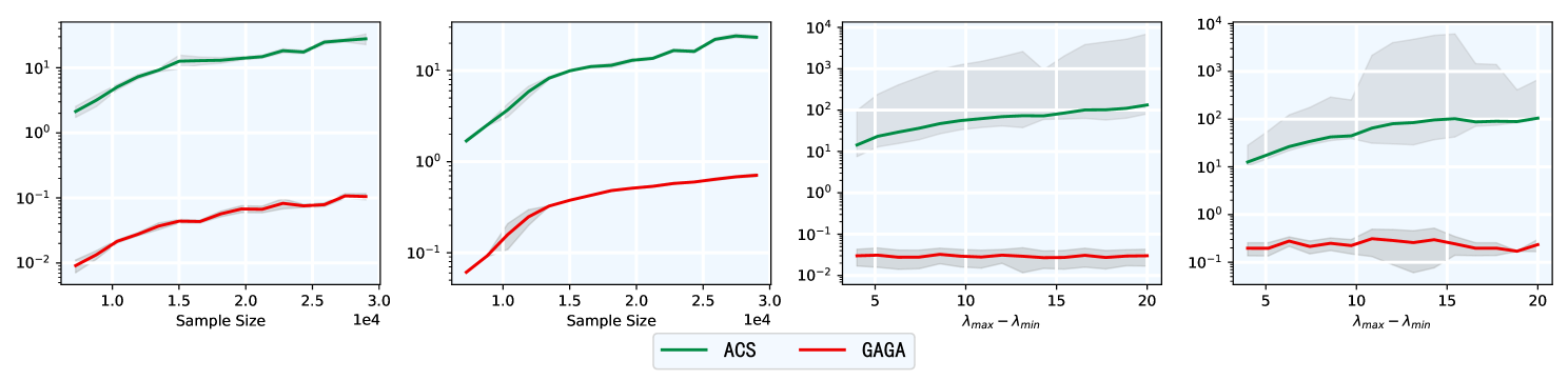
Figure 7: The study of efficiency comparison. $y$-axis denotes the average running time (in seconds) in 20 runs. The interval $[\lambda_{min},\lambda_{max}]$ refers to the predefined search space.

D.4 Path consistency

In this section we illustrate that the age-path tracked by GAGA exactly consists with the path of real partial optimum, which is produced by the ACS algorithm. Due to the expensive computational cost of finding the partial optimum using ACS (over 30 loops on average), we choose the toy datasets from the Scikit-learn package to trace and plot the age-path. In detail, we use the Boston house and breast cancer datasets for regression tasks, and the classification is performed on the handwritten digits dataset. In order to track the exact path of partial optimum, we set the step size to be 1e-4 and 3e-1 in ACS and GAGA, respectively. The graphs of the tracked path are illustrated in Figure 8, Figure 9 and Figure 10. The path of partial optimum is plotted in blue solid lines while the age-path traced by GAGA is marked with red dashed lines.

This result empirically validates the path consistency between the computed age-path by GAGA and the ground truth age-path (i.e. path of the partial optimum), which is stated in Theorem (3).

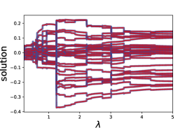
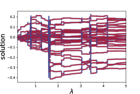
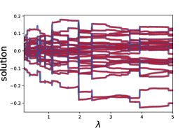
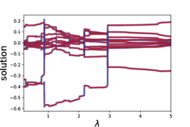
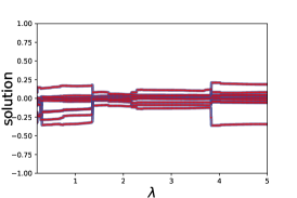
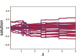
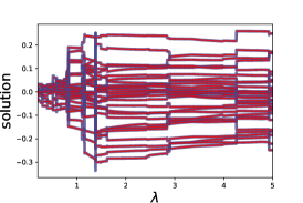
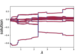
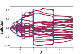
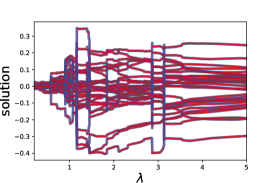
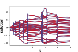
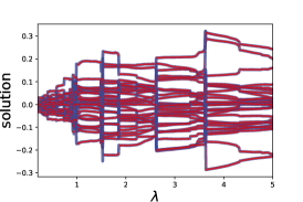
Figure 8: Age-path of SVM with different parameters and datasets. The first two rows of subfigures illustrate age-path using the linear SP-regularizer while the last two rows of subfigures show age-path using the mixture SP-regularizer. For experiments in the first and third row, the $\alpha=0.02$. For experiments in the second and fourth row, the $\alpha=0.04$.

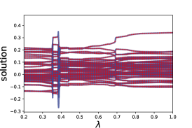
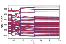
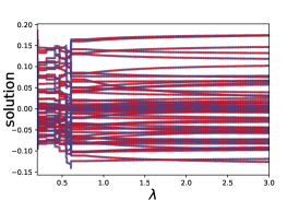
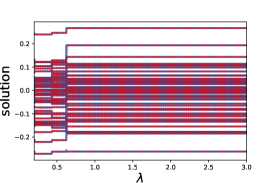
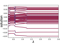
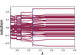
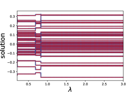
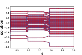
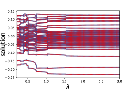
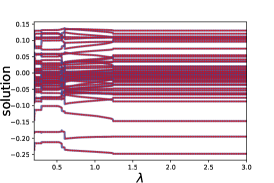
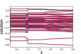
Figure 9: Age-path of Lasso with different parameters and datasets. The first two rows of subfigures illustrate age-path using the linear SP-regularizer while the last two rows of subfigures show age-path using the mixture SP-regularizer. For experiments in the first and third row, the $C=0.02$. For experiments in the second and fourth row, the $C=0.04$.

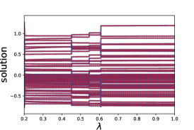
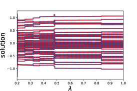
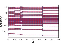
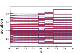
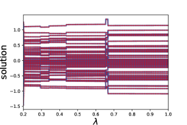
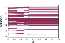
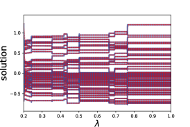
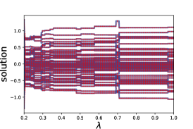
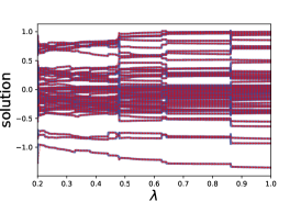
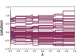
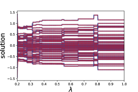
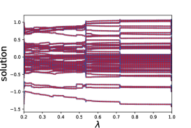
Figure 10: Age-path of logistic regression with different parameters and datasets. The first two rows of subfigures illustrate age-path using the linear SP-regularizer while the last two rows of subfigures show age-path using the mixture SP-regularizer. For experiments in the first and third row, the $C=25$. For experiments in the second and fourth row, the $C=40$.

D.5 More Histograms

We further show the intrinsic property of the age-path in more experiments. Specifically, we change the dataset, SP-regularizer as well as the value of other hyper-parameter in SVM, Lasso and logistic regression, while recording the number of different types of critical points. The results are illustrated in Figure 11, 12 and 13.

These histograms demonstrate that there exists more turning points on the age-path compared with the jump points. As a result, the heuristic technique applied in GAGA can avoid extensive unnecessary warm starts by identifying the exact type of each critical point.

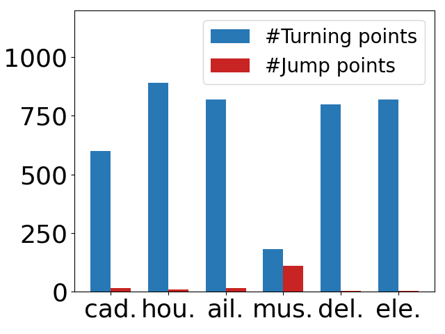
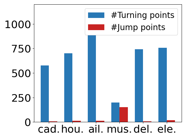
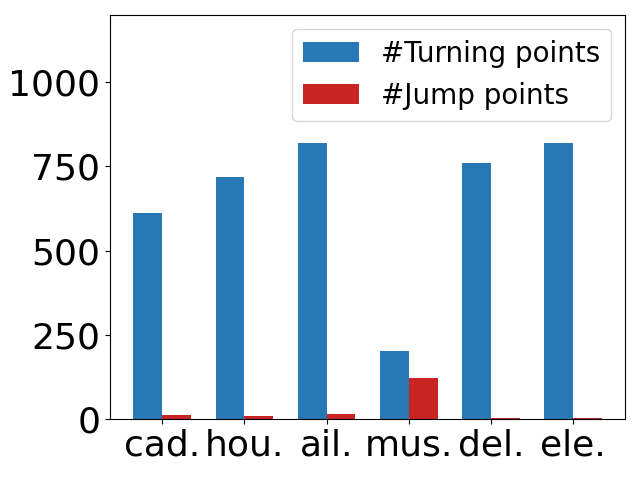
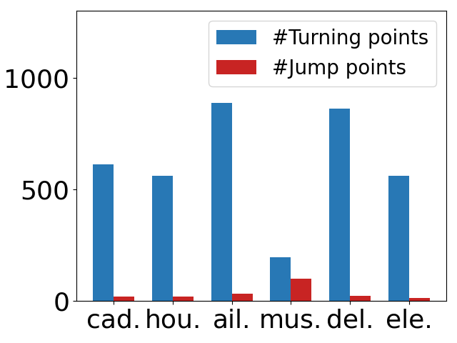
Figure 11: The number of different types of critical points in Lasso with different parameters and regularizers. The first row of subfigures illustrate different critical points in the age-path with linear SP-regularizer while the last row of figures show the number of different critical points in age-path using the mixture SP-regularizer.

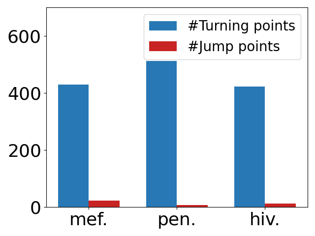
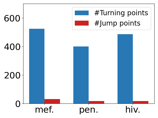
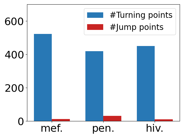
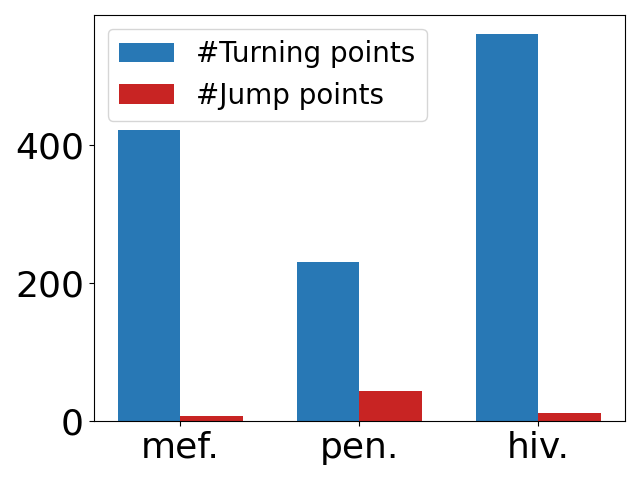
Figure 12: The number of different types of critical points in classic SVM with different parameters and regularizers.The first row of subfigures illustrate different critical points in the age-path with linear SP-regularizer while the last row of figures show the number of different critical points in age-path using the mixture SP-regularizer

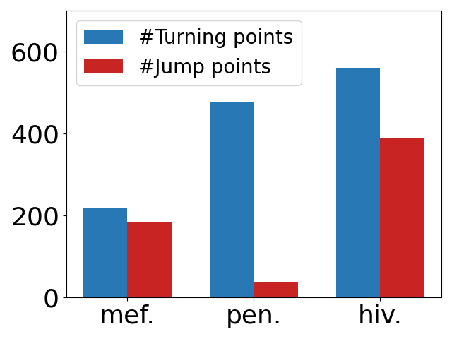
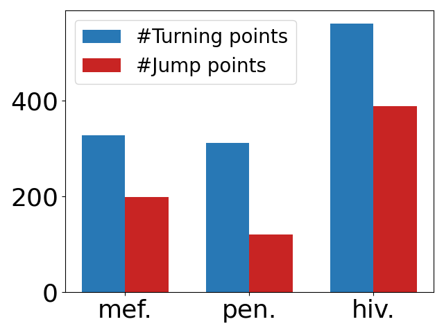
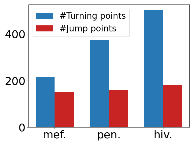
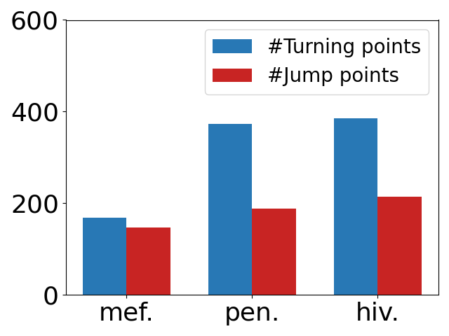
Figure 13: The number of different types of critical points in logistic regression with different parameters and regularizers. The first row of subfigures illustrate different critical points in the age path using linear SP-regularizer while the last row of subfigures show the number of different critical points in age-path using the mixture SP-regularizer.

D.6 Experimental Comparison of robust SVMs and Lasso

We also conduct a comparative study to the state-of-the-art robust model for SVMs [48, 49, 50] and Lasso [51] besides the SPL domain. Please take notice that RLSSVM and Re-LSSVM proposed by [48, 49] are variations of LS-SVM. Especially, we implement the Huber-loss Lasso as a special case of the generalized model proposed in [51]. The hyperparameters of these baselines are chosen from the best performance by grid search. All the experiments conducted on regression tasks are measured by the generalization error. We’d like to emphasize again that our GAGA framework pursues the best practice of conventional SPL while the SPL, as a special case of curriculum learning naturally owns certain shortcomings on the sample diversity [13]. Even subject to the inherent defects of vanilla SPL, the result in Table.7 reveals that our method still surpassed SOTA baselines in half of the experiments. The Table.8 further implies that GAGA outperforms the robust SVM in all conducted trails. These numerical results strongly validate the performance of our method under various noise levels.

Concretely speaking, the linear SP-regularizer is utilized in GAGA in the implementation. The $\gamma_{1}$ and $\gamma_{2}$ are hyperparameters of RLSSVM and RE-LSSVM. We use the same hyperparameters of GAGA in Appendix D.7.

Parameter						Huber Lasso		RLSSVM		Re-LSSVM		GAGA		Noise	Dataset
$e$	$\alpha$	$\sigma$	$\gamma_{1}$	$\theta$	$\gamma_{2}$	Mean	Std	Mean	Std	Mean	Std	Mean	Std
0.2	0.0006	0.7	1.9	0.2	1.9	0.399	0.003	0.449	0.107	0.318	0.010	0.491	0.001	0.1	ailerons
0.1	0.0001	0.8	1.9	0.4	1.8	0.410	0.003	0.573	0.082	0.499	0.010	0.49	0.002	0.2	ailerons
0.2	0.0016	0.5	1.9	0.2	1.9	0.407	0.003	0.419	0.079	0.696	0.018	0.489	0.002	0.3	ailerons
0.2	0.0006	0.7	1.9	0.9	1.8	0.428	0.005	0.500	0.050	0.877	0.014	0.491	0.001	0.4	ailerons
0.1	0.0008	0.8	1.9	0.2	1.9	0.452	0.003	0.705	0.052	1.118	0.017	0.491	0.001	0.5	ailerons
0.2	0.0018	0.8	1.9	0.3	1.7	0.478	0.003	0.565	0.044	1.159	0.025	0.490	0.015	0.6	ailerons
0.1	0.0002	0.8	1.9	0.2	1.7	0.180	0.000	0.207	0.082	0.315	0.024	0.201	0.046	0.2	houses
0.1	0.0013	0.5	1.9	0.9	1.8	0.182	0.000	0.206	0.042	0.343	0.170	0.221	0.015	0.3	houses
0.2	0.001	0.8	1.7	0.8	1.9	0.345	0.002	0.303	0.083	0.387	0.014	0.214	0.002	0.1	music
0.1	0.0013	0.5	1.9	0.6	1.9	0.365	0.001	0.315	0.011	0.486	0.013	0.213	0.005	0.2	music
0.2	0.0011	0.9	1.9	0.4	1.8	0.357	0.002	0.308	0.057	0.444	0.057	0.214	0.003	0.3	music
0.1	0.0019	1	1.9	0.4	1.7	0.406	0.003	0.422	0.087	0.412	0.015	0.211	0.008	0.4	music
0.2	0.0017	0.5	1.9	0.6	1.8	0.431	0.004	0.489	0.015	0.477	0.035	0.210	0.003	0.5	music
0.3	0.0011	0.8	1.9	0.3	1.9	0.484	0.005	0.598	0.017	0.521	0.019	0.214	0.001	0.6	music
0.1	0.0005	0.7	1.9	0.8	1.9	0.663	0.000	0.747	0.089	0.689	0.010	0.647	0.132	0.2	delta elevators
0.1	0.0014	0.8	1.9	0.4	1.8	0.666	0.000	0.744	0.025	0.694	0.033	0.634	0.132	0.3	delta elevators

Table 7: Average generalization erros with the standard deviation in 20 runs on different datasets. The top results in each row are in boldface.

Dataset	Parameter		Robust-SVM		GAGA		Noise Level
	C	$\gamma$	Mean	Std	Mean	Std
mfeat-pixel	1	0.8	0.948	0.001	0.980	0.006	0.1
mfeat-pixel	1	0.2	0.939	0.001	0.988	0.007	0.2
mfeat-pixel	1	0.7	0.927	0.002	0.980	0.015	0.3
pendigts	1	0.7	0.945	0.003	0.998	0.007	0.1
pendigts	1	0.6	0.944	0.002	0.995	0.004	0.2
pendigts	1	0.4	0.923	0.001	0.995	0.006	0.3

Table 8: Average classification accuracy with the standard deviation in 20 runs under different noise levels. The top results in each row are in boldface.

D.7 Sensitivity Analysis

In this subsection, we use the same settings except the backbone parameters $\alpha$, $C$ and the noise level. The linear SP-regularizer is utilized in GAGA. The classical SVM with linear kernel is chosen as the base model. Results in Table 9, 10, 11, 12 confirm the performances of competing methods with different backbone parameters while retaining the same noise level. Table 13, 14, 15, 16 display the running results under different noise levels while the other backbone parameters are kept. The results of the massive simulation studies again strongly demonstrate that our GAGA owns the best practice of the conventional SPL compared with the baseline methods, regardless of the specific parametric selections.

Dataset	Parameter	Competing Methods						Noise Level
	$\alpha$	ACS		MOSPL		GAGA
ailerons	0.001	0.494	0.001	0.493	0.008	0.490	0.001	0.3
ailerons	0.002	0.493	0.007	0.492	0.016	0.490	0.002	0.3
ailerons	0.003	0.493	0.001	0.493	0.001	0.489	0.002	0.3
ailerons	0.004	0.493	0.001	0.492	0.001	0.491	0.001	0.3
ailerons	0.005	0.493	0.001	0.493	0.001	0.49	0.001	0.3
ailerons	0.006	0.493	0.001	0.493	0.001	0.491	0.001	0.3
ailerons	0.007	0.494	0.002	0.492	0.002	0.491	0.001	0.3
ailerons	0.008	0.493	0.002	0.493	0.002	0.493	0.002	0.3
ailerons	0.009	0.493	0.002	0.493	0.002	0.493	0.002	0.3
ailerons	0.010	0.493	0.002	0.493	0.002	0.493	0.002	0.3
ailerons	0.011	0.493	0.002	0.493	0.002	0.493	0.002	0.3
ailerons	0.012	0.493	0.002	0.493	0.002	0.493	0.002	0.3
ailerons	0.013	0.493	0.002	0.493	0.002	0.493	0.002	0.3
ailerons	0.014	0.493	0.002	0.493	0.002	0.493	0.002	0.3
ailerons	0.015	0.493	0.002	0.493	0.002	0.493	0.002	0.3

Table 9: Average generalization errors and the standard deviation in 20 runs with different values of $\alpha$. The top results in each row are in boldface.

Dataset	Parameter	Competing Methods						Noise Level
	$\alpha$	ACS		MOSPL		GAGA
music	0.001	0.230	0.011	0.226	0.009	0.227	0.011	0.3
music	0.002	0.224	0.005	0.222	0.006	0.218	0.004	0.3
music	0.003	0.227	0.011	0.223	0.008	0.219	0.009	0.3
music	0.004	0.221	0.011	0.219	0.010	0.213	0.009	0.3
music	0.005	0.221	0.005	0.220	0.004	0.209	0.005	0.3
music	0.006	0.218	0.009	0.216	0.009	0.213	0.027	0.3
music	0.007	0.222	0.003	0.215	0.005	0.211	0.004	0.3
music	0.008	0.215	0.004	0.213	0.003	0.208	0.002	0.3
music	0.009	0.216	0.006	0.213	0.005	0.207	0.003	0.3
music	0.010	0.216	0.007	0.214	0.007	0.208	0.003	0.3
music	0.011	0.215	0.008	0.212	0.006	0.206	0.005	0.3
music	0.012	0.211	0.007	0.208	0.007	0.205	0.005	0.3
music	0.013	0.210	0.005	0.210	0.003	0.207	0.003	0.3
music	0.014	0.212	0.004	0.208	0.005	0.206	0.003	0.3
music	0.015	0.211	0.006	0.210	0.004	0.207	0.003	0.3
music	0.016	0.211	0.006	0.211	0.007	0.206	0.004	0.3
music	0.017	0.207	0.004	0.207	0.006	0.205	0.004	0.3
music	0.018	0.210	0.006	0.206	0.007	0.205	0.005	0.3
music	0.019	0.210	0.006	0.208	0.007	0.206	0.003	0.3
music	0.020	0.206	0.003	0.206	0.003	0.206	0.003	0.3
music	0.021	0.207	0.005	0.207	0.005	0.205	0.003	0.3
music	0.022	0.207	0.004	0.207	0.003	0.205	0.002	0.3
music	0.023	0.206	0.004	0.205	0.003	0.205	0.003	0.3
music	0.024	0.206	0.003	0.207	0.005	0.205	0.004	0.3
music	0.025	0.207	0.003	0.207	0.003	0.204	0.003	0.3
music	0.026	0.206	0.002	0.206	0.003	0.206	0.003	0.3
music	0.027	0.208	0.004	0.206	0.004	0.205	0.004	0.3
music	0.028	0.208	0.005	0.208	0.005	0.205	0.004	0.3
music	0.029	0.205	0.005	0.205	0.005	0.205	0.003	0.3
music	0.03	0.207	0.004	0.207	0.004	0.205	0.002	0.3

Table 10: Average generalization errors and the standard deviation in 20 runs with different values of $\alpha$. The top results in each row are in boldface.

Dataset	Parameter	Competing Methods						Noise Level
	C	ACS		MOSPL		GAGA
mfeat-pixel	0.100	0.932	0.012	0.959	0.005	0.965	0.005	0.3
mfeat-pixel	0.200	0.929	0.009	0.957	0.006	0.966	0.003	0.3
mfeat-pixel	0.300	0.937	0.054	0.962	0.281	0.980	0.015	0.3
mfeat-pixel	0.400	0.936	0.011	0.966	0.013	0.979	0.014	0.3
mfeat-pixel	0.500	0.928	0.008	0.951	0.004	0.961	0.005	0.3
mfeat-pixel	0.600	0.933	0.008	0.960	0.006	0.967	0.004	0.3
mfeat-pixel	0.700	0.922	0.012	0.946	0.006	0.948	0.005	0.3
mfeat-pixel	0.800	0.927	0.014	0.952	0.008	0.960	0.002	0.3
mfeat-pixel	0.900	0.927	0.006	0.945	0.010	0.955	0.010	0.3
mfeat-pixel	1.000	0.925	0.007	0.948	0.006	0.951	0.001	0.3
mfeat-pixel	1.100	0.928	0.009	0.952	0.006	0.955	0.002	0.3
mfeat-pixel	1.200	0.933	0.018	0.961	0.009	0.972	0.005	0.3
mfeat-pixel	1.300	0.929	0.011	0.953	0.009	0.964	0.004	0.3
mfeat-pixel	1.400	0.934	0.007	0.966	0.013	0.971	0.004	0.3
mfeat-pixel	1.500	0.936	0.007	0.958	0.013	0.978	0.003	0.3
mfeat-pixel	1.600	0.920	0.007	0.923	0.007	0.945	0.004	0.3
mfeat-pixel	1.700	0.931	0.010	0.948	0.014	0.969	0.004	0.3
mfeat-pixel	1.800	0.934	0.015	0.963	0.015	0.970	0.005	0.3
mfeat-pixel	1.900	0.929	0.007	0.957	0.006	0.962	0.007	0.3

Table 11: Average classification accuracy and the standard deviation in 20 runs with different values of C. The top results in each row are in boldface.

Dataset	Parameter	Competing Methods						Noise Level
	C	ACS		MOSPL		GAGA
pendigts	0.100	0.984	0.003	0.984	0.006	0.998	0.007	0.3
pendigts	0.200	0.989	0.003	0.991	0.008	0.995	0.004	0.3
pendigts	0.3	0.983	0.004	0.989	0.009	0.995	0.006	0.3
pendigts	0.400	0.985	0.002	0.988	0.007	0.992	0.006	0.3
pendigts	0.500	0.982	0.005	0.983	0.005	0.993	0.004	0.3
pendigts	0.600	0.987	0.007	0.989	0.010	0.992	0.004	0.3
pendigts	0.700	0.986	0.007	0.988	0.006	0.996	0.002	0.3
pendigts	0.800	0.979	0.003	0.987	0.009	0.995	0.007	0.3
pendigts	0.900	0.987	0.003	0.985	0.011	0.991	0.005	0.3
pendigts	1.000	0.989	0.006	0.986	0.012	0.992	0.006	0.3
pendigts	1.100	0.982	0.005	0.987	0.005	0.990	0.554	0.3
pendigts	1.200	0.983	0.008	0.982	0.007	0.994	0.004	0.3
pendigts	1.300	0.981	0.006	0.991	0.007	0.995	0.004	0.3
pendigts	1.400	0.980	0.003	0.983	0.002	0.989	0.005	0.3
pendigts	1.500	0.981	0.007	0.986	0.006	0.995	0.002	0.3
pendigts	1.600	0.981	0.009	0.985	0.011	0.992	0.003	0.3
pendigts	1.700	0.979	0.006	0.981	0.004	0.995	0.006	0.3
pendigts	1.800	0.977	0.004	0.983	0.005	0.993	0.006	0.3

Table 12: Average classification accuracy and the standard deviation in 20 runs with different values of C. The top results in each row are in boldface.

Dataset	Parameter	Competing Methods						Noise Level
	$\alpha$	ACS		MOSPL		GAGA
ailerons	0.006	0.492	0.001	0.492	0.005	0.491	0.001	0.1
ailerons	0.006	0.492	0.001	0.491	0.016	0.49	0.002	0.2
ailerons	0.006	0.493	0.001	0.493	0.001	0.489	0.002	0.3
ailerons	0.006	0.493	0.001	0.492	0.001	0.491	0.001	0.4
ailerons	0.006	0.493	0.001	0.493	0.001	0.491	0.001	0.5
ailerons	0.006	0.493	0.001	0.492	0.001	0.491	0.001	0.6
ailerons	0.006	0.494	0.002	0.492	0.002	0.491	0.001	0.7
ailerons	0.006	0.493	0.002	0.493	0.002	0.493	0.002	0.8

Table 13: Average generalization errors with the standard deviation in 20 runs under different noise levels. The top results in each row are in boldface.

Dataset	Parameter	Competing Methods						Noise Level
	$\alpha$	ACS		MOSPL		GAGA
music	0.006	0.22	0.004	0.219	0.003	0.214	0.002	0.1
music	0.006	0.218	0.005	0.215	0.016	0.213	0.005	0.2
music	0.006	0.221	0.009	0.217	0.006	0.214	0.003	0.3
music	0.006	0.226	0.011	0.221	0.01	0.211	0.008	0.4
music	0.006	0.228	0.011	0.22	0.006	0.21	0.003	0.5
music	0.006	0.493	0.001	0.492	0.001	0.491	0.001	0.6
music	0.006	0.494	0.002	0.492	0.002	0.491	0.001	0.7
music	0.006	0.493	0.002	0.493	0.002	0.493	0.002	0.8

Table 14: Average generalization errors with the standard deviation in 20 runs under different noise levels. The top results in each row are in boldface.

Dataset	Parameter	Competing Methods						Noise Level
	C	ACS		MOSPL		GAGA
mfeat-pixel	1.000	0.946	0.018	0.967	0.007	0.980	0.006	0.1
mfeat-pixel	1.000	0.949	0.016	0.978	0.013	0.988	0.007	0.2
mfeat-pixel	1.000	0.937	0.054	0.962	0.281	0.980	0.015	0.3
mfeat-pixel	1.000	0.939	0.011	0.955	0.012	0.968	0.010	0.4
mfeat-pixel	1.000	0.941	0.008	0.962	0.005	0.972	0.008	0.5
mfeat-pixel	1.000	0.946	0.011	0.971	0.006	0.978	0.006	0.6
mfeat-pixel	1.000	0.934	0.013	0.955	0.005	0.959	0.005	0.7

Table 15: Average classification accuracy with the standard deviation in 20 runs under different noise levels. The top results in each row are in boldface.

Dataset	Parameter	Competing Methods						Noise Level
	C	ACS		MOSPL		GAGA
pendigts	1.000	0.979	0.012	0.984	0.006	0.994	0.004	0.1
pendigts	1.000	0.980	0.003	0.991	0.008	0.998	0.004	0.2
pendigts	1.000	0.989	0.006	0.986	0.012	0.992	0.006	0.3
pendigts	1.000	0.980	0.009	0.990	0.005	0.996	0.006	0.4
pendigts	1.000	0.974	0.004	0.994	0.005	0.994	0.004	0.5
pendigts	1.000	0.984	0.007	0.986	0.010	0.996	0.004	0.6
pendigts	1.000	0.970	0.007	0.972	0.006	0.974	0.006	0.7

Table 16: Average classification accuracy with the standard deviation in 20 runs under different noise levels. The top results in each row are in boldface.

Appendix E Limitations and Broader Impact

Limitations.

The current framework GAGA is only applicable to the vanilla SPL paradigm, while some variants of SPL (e.g., self-paced learning with diversity [2]) could have a group of hyperparameters more than the mere $\lambda$. In this instance, the original solution paths escalates into the solution surfaces, and made it harder to track the solutions. Another point is that our argument assumed that the target function is a biconvex problem, while many complex losses (e.g., deep neural networks) could be the function of strongly non-convex.

Broader Impact.

The parties with limited computational resource may benefit from the efficiency of our proposed work. Meanwhile, the research groups that sensitive to age parameters in SPL may benefit from the robustness of our work. For social impact, our work improve the hyperparameter search and helps reducing the computation cost, which saves carbon emissions during the training process.

Appendix F Code Readme

This section explains how to use the code implementing the proposed GAGA.

F.1 Archive content

1. The fundamental implementation of our methodology GAGA is called GAGA.py, which includes all the functions used in our experiment. In more detail, they are named in the form of [GAGA]_[Model_Name]_[SPL_Regularizer], e.g., GAGA_svm_linear.

2. The Evaluation.py provides functions for evaluating solution path from different models including ACS.

3. The Input_Data.py offers file-IO for all datasets used in our experiment.

4. The ACS.py provides ACS algorithm for solving SPL.

F.2 Reproducing the results of the article

For the sake of quick and convenient reproducing experiments and checking our findings, we provide a demo named main.py. We use open-source datasets and provide file-IO functions along with detailed pre-processing pipeline for users. Any used datasets in our experiment can be easily downloaded them from the UCI and OpenML website and put them in the datasets folder. The required dependencies and running environment is recorded in Environment.txt.

References

- [1] M. Kumar, Ben Packer, and Daphne Koller. Self-paced learning for latent variable models. pages 1189–1197, 01 2010.
- [2] Lu Jiang, Deyu Meng, Shoou-I Yu, Zhenzhong Lan, Shiguang Shan, and Alexander Hauptmann. Self-paced learning with diversity. Advances in neural information processing systems, 27, 2014.
- [3] Qian Zhao, Deyu Meng, Lu Jiang, Qi Xie, Zongben Xu, and Alexander G Hauptmann. Self-paced learning for matrix factorization. In Twenty-ninth AAAI conference on artificial intelligence, 2015.
- [4] Fan Ma, Deyu Meng, Qi Xie, Zina Li, and Xuanyi Dong. Self-paced co-training. In International Conference on Machine Learning, pages 2275–2284. PMLR, 2017.
- [5] Liang Lin, Keze Wang, Deyu Meng, Wangmeng Zuo, and Lei Zhang. Active self-paced learning for cost-effective and progressive face identification. IEEE transactions on pattern analysis and machine intelligence, 40(1):7–19, 2017.
- [6] Kamran Ghasedi, Xiaoqian Wang, Cheng Deng, and Heng Huang. Balanced self-paced learning for generative adversarial clustering network. In Proceedings of the IEEE/CVF Conference on Computer Vision and Pattern Recognition, pages 4391–4400, 2019.
- [7] Hongchang Gao and Heng Huang. Self-paced network embedding. In Proceedings of the 24th ACM SIGKDD International Conference on Knowledge Discovery & Data Mining, pages 1406–1415, 2018.
- [8] Jiangzhang Gan, Guoqiu Wen, Hao Yu, Wei Zheng, and Cong Lei. Supervised feature selection by self-paced learning regression. Pattern Recognition Letters, 132:30–37, 2020.
- [9] James S Supancic and Deva Ramanan. Self-paced learning for long-term tracking. In Proceedings of the IEEE conference on computer vision and pattern recognition, pages 2379–2386, 2013.
- [10] Lili Pan, Shijie Ai, Yazhou Ren, and Zenglin Xu. Self-paced deep regression forests with consideration on underrepresented examples. In European Conference on Computer Vision, pages 271–287. Springer, 2020.
- [11] Xiaoping Wu, Jianlong Chang, Yu-Kun Lai, Jufeng Yang, and Qi Tian. Bispl: Bidirectional self-paced learning for recognition from web data. IEEE Transactions on Image Processing, 30:6512–6527, 2021.
- [12] Yoshua Bengio, Jérôme Louradour, Ronan Collobert, and Jason Weston. Curriculum learning. In Proceedings of the 26th annual international conference on machine learning, pages 41–48, 2009.
- [13] Petru Soviany, Radu Tudor Ionescu, Paolo Rota, and Nicu Sebe. Curriculum learning: A survey. International Journal of Computer Vision, pages 1–40, 2022.
- [14] Lu Jiang, Deyu Meng, Qian Zhao, Shiguang Shan, and Alexander G Hauptmann. Self-paced curriculum learning. In Twenty-Ninth AAAI Conference on Artificial Intelligence, 2015.
- [15] Deyu Meng, Qian Zhao, and Lu Jiang. A theoretical understanding of self-paced learning. Information Sciences, 414:319–328, 2017.
- [16] Lu Jiang, Deyu Meng, Teruko Mitamura, and Alexander G Hauptmann. Easy samples first: Self-paced reranking for zero-example multimedia search. In Proceedings of the 22nd ACM international conference on Multimedia, pages 547–556, 2014.
- [17] Fan Ma, Deyu Meng, Xuanyi Dong, and Yi Yang. Self-paced multi-view co-training. Journal of Machine Learning Research, 2020.
- [18] Jiangtao Peng, Weiwei Sun, and Qian Du. Self-paced joint sparse representation for the classification of hyperspectral images. IEEE Transactions on Geoscience and Remote Sensing, 57(2):1183–1194, 2018.
- [19] Maoguo Gong, Hao Li, Deyu Meng, Qiguang Miao, and Jia Liu. Decomposition-based evolutionary multiobjective optimization to self-paced learning. IEEE Transactions on Evolutionary Computation, 23(2):288–302, 2018.
- [20] Richard E Wendell and Arthur P Hurter Jr. Minimization of a non-separable objective function subject to disjoint constraints. Operations Research, 24(4):643–657, 1976.
- [21] James Bergstra, Rémi Bardenet, Yoshua Bengio, and Balázs Kégl. Algorithms for hyper-parameter optimization. Advances in neural information processing systems, 24, 2011.
- [22] Jonathan F Bard. Practical bilevel optimization: algorithms and applications, volume 30. Springer Science & Business Media, 2013.
- [23] Bradley Efron, Trevor Hastie, Iain Johnstone, and Robert Tibshirani. Least angle regression. The Annals of statistics, 32(2):407–499, 2004.
- [24] Trevor Hastie, Saharon Rosset, Robert Tibshirani, and Ji Zhu. The entire regularization path for the support vector machine. Journal of Machine Learning Research, 5(Oct):1391–1415, 2004.
- [25] William Karush. Minima of functions of several variables with inequalities as side constraints. M. Sc. Dissertation. Dept. of Mathematics, Univ. of Chicago, 1939.
- [26] Ryan J Tibshirani and Jonathan Taylor. The solution path of the generalized lasso. The annals of statistics, 39(3):1335–1371, 2011.
- [27] Kohei Ogawa, Motoki Imamura, Ichiro Takeuchi, and Masashi Sugiyama. Infinitesimal annealing for training semi-supervised support vector machines. In International Conference on Machine Learning, pages 897–905. PMLR, 2013.
- [28] Bin Gu and Victor S Sheng. A solution path algorithm for general parametric quadratic programming problem. IEEE transactions on neural networks and learning systems, 29(9):4462–4472, 2017.
- [29] Hao Li, Maoguo Gong, Deyu Meng, and Qiguang Miao. Multi-objective self-paced learning. In Thirtieth AAAI conference on artificial intelligence, 2016.
- [30] Hao Li, Maoguo Gong, Congcong Wang, and Qiguang Miao. Pareto self-paced learning based on differential evolution. IEEE Transactions on Cybernetics, 2019.
- [31] Bin Gu, Zhou Zhai, Xiang Li, and Heng Huang. Finding age path of self-paced learning. In 2021 IEEE International Conference on Data Mining (ICDM), pages 151–160. IEEE, 2021.
- [32] Bin Gu, Xiao-Tong Yuan, Songcan Chen, and Heng Huang. New incremental learning algorithm for semi-supervised support vector machine. In Proceedings of the 24th ACM SIGKDD International Conference on Knowledge Discovery & Data Mining, pages 1475–1484, 2018.
- [33] Vladimir Vapnik. The nature of statistical learning theory. Springer science & business media, 1999.
- [34] Robert Tibshirani. Regression shrinkage and selection via the lasso. Journal of the Royal Statistical Society: Series B (Methodological), 58(1):267–288, 1996.
- [35] Deyu Meng, Qian Zhao, and Lu Jiang. What objective does self-paced learning indeed optimize? arXiv preprint arXiv:1511.06049, 2015.
- [36] Guoqi Li, Changyun Wen, Wei Xing Zheng, and Guangshe Zhao. Iterative identification of block-oriented nonlinear systems based on biconvex optimization. Systems & Control Letters, 79:68–75, 2015.
- [37] Jochen Gorski, Frank Pfeuffer, and Kathrin Klamroth. Biconvex sets and optimization with biconvex functions: a survey and extensions. Mathematical methods of operations research, 66(3):373–407, 2007.
- [38] Zilu Ma, Shiqi Liu, Deyu Meng, Yong Zhang, SioLong Lo, and Zhi Han. On convergence properties of implicit self-paced objective. Information Sciences, 462:132–140, 2018.
- [39] Michael Held, Philip Wolfe, and Harlan P Crowder. Validation of subgradient optimization. Mathematical programming, 6(1):62–88, 1974.
- [40] Bennet Gebken, Katharina Bieker, and Sebastian Peitz. On the structure of regularization paths for piecewise differentiable regularization terms. arXiv preprint arXiv:2111.06775, 2021.
- [41] Barrett O’neill. Elementary differential geometry. Elsevier, 2006.
- [42] Bernhard Schölkopf. The kernel trick for distances. Advances in neural information processing systems, 13, 2000.
- [43] Arthur Asuncion and David Newman. Uci machine learning repository, 2007.
- [44] Joaquin Vanschoren, Jan N Van Rijn, Bernd Bischl, and Luis Torgo. Openml: networked science in machine learning. ACM SIGKDD Explorations Newsletter, 15(2):49–60, 2014.
- [45] Benoît Frénay and Michel Verleysen. Classification in the presence of label noise: A survey. Neural Networks and Learning Systems, IEEE Transactions on, 25:845–869, 05 2014.
- [46] Aritra Ghosh, Himanshu Kumar, and P. Sastry. Robust loss functions under label noise for deep neural networks. 12 2017.
- [47] Matthew Jagielski, Alina Oprea, Battista Biggio, Chang Liu, Cristina Nita-Rotaru, and Bo Li. Manipulating machine learning: Poisoning attacks and countermeasures for regression learning. pages 19–35, 05 2018.
- [48] Chuanfa Chen, Changqing Yan, and Yanyan Li. A robust weighted least squares support vector regression based on least trimmed squares. Neurocomputing, 168:941–946, 2015.
- [49] Xiaowei Yang, Liangjun Tan, and Lifang He. A robust least squares support vector machine for regression and classification with noise. Neurocomputing, 140:41–52, 2014.
- [50] Battista Biggio, Blaine Nelson, and Pavel Laskov. Support vector machines under adversarial label noise. In Asian conference on machine learning, pages 97–112. PMLR, 2011.
- [51] Nasser Nasrabadi, Trac Tran, and Nam Nguyen. Robust lasso with missing and grossly corrupted observations. Advances in Neural Information Processing Systems, 24, 2011.
- [52] Adi Ben-Israel and T Greville. Generalized Inverse: Theory and Application. 01 1974.
- [53] Roger A. Horn and Charles R. Johnson. Matrix Analysis. Cambridge University Press, 1990.
- [54] Krishnan Radhakrishnan and Alan Hindmarsh. Description and use of lsode, the livermore solver for ordinary differential equations. 01 1994.
- [55] J. Watt. Numerical initial value problems in ordinary differential equations. The Computer Journal, 15:155–155, 05 1972.
- [56] William Adkins and Mark Davidson. Ordinary Differential Equations. 01 2012.
- [57] F. Pedregosa, G. Varoquaux, A. Gramfort, V. Michel, B. Thirion, O. Grisel, M. Blondel, P. Prettenhofer, R. Weiss, V. Dubourg, J. Vanderplas, A. Passos, D. Cournapeau, M. Brucher, M. Perrot, and E. Duchesnay. Scikit-learn: Machine learning in Python. Journal of Machine Learning Research, 12:2825–2830, 2011.
- [58] et.al. Jazzbin. geatpy: The genetic and evolutionary algorithm toolbox with high performance in python, 2020.