Fair Inference for Discrete Latent Variable Models

Abstract

It is now well understood that machine learning models, trained on data without due care, often exhibit unfair and discriminatory behavior against certain populations. Traditional algorithmic fairness research has mainly focused on supervised learning tasks, particularly classification. While fairness in unsupervised learning has received some attention, the literature has primarily addressed fair representation learning of continuous embeddings. In this paper, we conversely focus on unsupervised learning using probabilistic graphical models with discrete latent variables. We develop a fair stochastic variational inference technique for the discrete latent variables, which is accomplished by including a fairness penalty on the variational distribution that aims to respect the principles of intersectionality, a critical lens on fairness from the legal, social science, and humanities literature, and then optimizing the variational parameters under this penalty. We first show the utility of our method in improving equity and fairness for clustering using naïve Bayes and Gaussian mixture models on benchmark datasets. To demonstrate the generality of our approach and its potential for real-world impact, we then develop a special-purpose graphical model for criminal justice risk assessments, and use our fairness approach to prevent the inferences from encoding unfair societal biases.

Keywords AI fairness  $\cdot$ Latent variable models  $\cdot$ Variational inference  $\cdot$ Intersectionality

1 Introduction

In our interconnected world, artificial intelligence (AI) and machine learning (ML) have become ubiquitous. Increasingly, the automated decisions made by these systems have important real-life consequences, from credit scoring and subsequent lending outcomes, to college admissions, to career recommendations, to the prediction of re-offending [1, 2]. However, the integrity of these decisions can often be undermined by implicit bias or societal stereotypes in the underlying data, leading the behavior of these learning algorithms to unfairly discriminate against certain groups of people, including women, people of color, and individuals on the LGBTQA spectrum[3, 4, 5, 1, 2, 6, 7].

With the rising awareness and regulations, the AI community has devoted much effort to the development and enforcement of numerous quantifiable notions of fairness for AI/ML models [8, 9, 10, 11, 12, 13, 14]. The main paradigm for fair algorithms is to posit a mathematical criteria of fairness across protected demographic groups, (e.g. by gender, race, and age) or similar individuals (e.g. persons with similar merits and risks) [15, 16]. The paradigm then enforces these criteria, when optimizing objective functions, by penalizing violations [17, 13, 18] or by imposing constraints [19] or by finding a transformation of data that provides fair latent representations [9, 20, 21, 22, 23, 24].

From a fairness perspective, representation learning is appealing because deep learning-based vector representations often generalize to tasks which are unspecified at training time, implying that a properly designed fair network might operate as a kind of “parity bottleneck,” reducing discrimination in unknown downstream tasks [25]. Particularly, the goal of fair representation learning is to transform the data into continuous latent spaces that are invariant to protected attributes and useful to mitigate societal bias in different downstream tasks, e.g., classification [26, 27]. Most of the recent frameworks [21, 28, 25, 27] are built upon the variational autoencoder (VAE) [29, 30], which can perform effective stochastic variational inference (SVI)[31] and learning in continuous latent variable models using backpropagation.

While the benefits of fair representations in continuous latent space in downstream tasks are clear, we are conversely interested in extending the success of variational techniques to fair inference in graphical models with discrete latent variables. As societal prejudices, societal disadvantages, underrepresentation of minorities, intentional prejudices and proxy variables are inherent in historical data [4], inferences can naturally encode these harmful biases in the latent variables which should be prevented to mitigate discriminatory decisions. Such graphical models are used in numerous AI/ML methods including semi-supervised learning [32], binary latent attribute models [33], hard attention models [34], clustering [35], and topic modeling [36]. Furthermore, discrete latent variables are a natural fit for complex reasoning, planning and predictive learning, e.g., “if you study hard, you will be successful.” However, inference on discrete latent variables with backpropagation-based variational methods is difficult because of the inability to re-parameterize gradients [33, 37, 38, 39]. To address this, continuous relaxations in the VAE framework have been found effective using the Gumbel-Softmax re-parameterization trick [40, 41] which defines a temperature-based continuous distribution, and converges to a discrete distribution in the zero-temperature limit. Chierichetti et al. [42] and Backurs et al. [43] addressed fairness in clustering problems for both k-center and k-median objectives, but not for the general case of graphical models with discrete latents. Fairness approaches exist for causal latent variable models [11, 44], however, these models enforce fair causal inference in a supervised setting (e.g. with a class label).

In this paper, we develop a practical framework for fair SVI on arbitrary graphical models with discrete latent variables to improve their equity and fairness. Our method is general and could be incorporated into probabilistic programming systems without additional assumptions. Given a probabilistic graphical model, e.g. a custom model defined for a particular task, our goal is to perform inference such that the results do not reflect negative stereotypes or bias. For example, multiple studies demonstrated that police stop people from racial and ethnic minority groups more frequently than whites [45, 46, 47, 48, 49]. In a traffic model, we may wish to prevent the inference that individuals of one demographic drive more aggressively than other demographics. Such an inference may in fact be warranted by the data, but it may be known –due to knowledge not encoded in the data, or known causes of the issue such as less data for minorities– that this inference cannot be correct, or it may be desirable to prevent it in order to avoid harm due to the use of the model, pursuant to Title VII [4]. Furthermore, our fairness intervention technique enforces an intersectional fairness notion [13] that guarantees fairness protections for all subsets of the protected attributes (e.g., black women, women, and black) which is consistent with the ethical principles of intersectionality theory [50, 51].

Our key contributions can be summarized as follows:

• We develop a method for ensuring intersectional fairness in stochastic variational inference for unsupervised discrete latent variable models.

• We demonstrate the utility of our method for clustering analysis using naïve Bayes and Gaussian mixture models on fairness benchmark datasets.

• We show our method’s generality by applying it to fair inference in a new special-purpose model for criminal justice decisions based on COMPAS [3].

2 Background

2.1 Problem Setup: Fair Latent Variable Modeling

We assume a generative model $p(x,z)=p(x|z)p(z)$ that produces a dataset $\mathbf{x}=\{x_{j}\}_{j=1}^{n}$ consisting of $n$ i.i.d. individuals, generated using a set of $K$-dimensional discrete latent variables $\mathbf{z}=\{z_{j}\}_{j=1}^{n}$. Let $A$ be protected attributes, e.g. the individuals’ gender and race, which may or may not be included in the typical (or non-sensitive) $D$-dimensional attribute vector $x$. Furthermore, each $z_{j}$ is assumed to be generated from some prior distribution $p(z)$. Variational inference [52, 53, 54, 31] is an optimization approach to solve inference problems for latent variable models. We aim to compute the posterior distribution $p(z|x)$, which is assumed intractable over latent variables, and so approximation techniques must be used. The key idea is to approximate $p(z|x)$ with a more tractable distribution $q(z)$, referred to as a variational distribution, and minimize the KL-divergence $D_{KL}$ between them.

2.2 Variational Autoencoder (VAE)

The variational autoencoder (VAE) [29] performs variational inference in a latent Gaussian model where the variational posterior and model likelihood are parameterized by neural nets $\phi$ and $\theta$, respectively. Kingma and Welling [29] developed a differentiable reparameterization technique for efficient SVI for probabilistic models in the presence of continuous latent variables $z$. The VAE is generally implemented with a Gaussian prior $p_{\theta}(z)=\mathcal{N}(0,1)$. The objective is to maximize the evidence lower-bound (ELBO):

$$\mathcal{L}_{\text{VAE}}(\theta,\phi)=\mathbb{E}_{q_{\phi}(z|x)}[\log p_{\theta}(x|z)]-D_{KL}[q_{\phi}(z|x)||p_{\theta}(z)]\mbox{ .}$$ (1)

The objective to maximize $\mathcal{L}_{\text{VAE}}$ is made differentiable by reparameterizing $z\sim q_{\phi}(z|x)$, which is here assumed to be Gaussian, with $z=\mu+\sigma\odot\mathcal{E}$, where $\mathcal{E}\sim\mathcal{N}(0,1)$.

2.3 The Gumbel-Softmax Reparameterization Trick

Jang et al. [40] and Maddison et al. [41] introduced a reparameterization technique for training VAEs with discrete latent variables using the Gumbel-Max trick [55, 56], which provides an efficient way to draw samples $z$ from a $k$-dimensional categorical distribution with class probabilities $\pi$ as $z=\text{one\_hot}({\text{arg max}_{i}}[g_{i}+\log\pi_{i}])$, where $g_{i}\sim\text{Gumbel}(0,1)$ are i.i.d. samples. As “arg max" is not differentiable, the softmax function is used to approximate it:

$$z_{i}=\frac{\text{exp}((g_{i}+\log\pi_{i})/\tau)}{\sum_{k=1}^{K}\text{exp}((g_{k}+\log\pi_{k})/\tau)}\quad\quad\text{for }i=1,\dots,K\mbox{ ,}$$ (2)

where the temperature $\tau$, which controls how closely samples from the Gumbel-Softmax distribution approximate those from the discrete distribution, is annealed towards $0$ during training.

3 Method: VI with a Fairness Intervention

We aim to perform fair inference on a generative probabilistic model $p_{\theta}(x,z)$ with discrete latent variables $z$. We desire a stochastic variational inference algorithm to compute the posterior distribution $p_{\theta}(z|x)$ which achieves two properties: 1) inference that scales to the big data, and 2) a simple and efficient fairness intervention using backpropagation.

3.1 Inference Network

Following Kingma and Welling [29], we use a neural network-based inference network $q_{\phi}(z|x)$ for the variational approximation to the intractable posterior $p_{\theta}(z|x)$, where weights and biases of the neural network are variational parameters $\phi$. Following Jang et al. [40], let the prior $p_{\theta}(z)$ be a discrete distribution with uniform probability $1/K$, although this can easily be generalized as shown in a later section for special purpose modeling. The first step of our method is to reparameterize the variational distribution for the purposes of sampling latent variables so that discrete distributions are re-represented as unconstrained distributions, in order to facilitate backpropagation on these variables. The two main options are the logistic-normal representation [36], and the Gumbel-softmax representation [40, 41]. If we use the logistic-normal representation, we reparameterize $q_{\phi}(z|x)$ using a mean $\mu$ and covariance matrix $\Sigma$ via a logistic function. We focus on the Gumbel-softmax approach, since it performed better in preliminary experiments. To encode discrete $z$, the inference network basically outputs unnormalized log probabilities $\log\pi$ for the latent classes which are then used to reparameterize $q_{\phi}(z|x)$ using the Gumbel-Softmax trick in Equation 2.

3.2 Generative Network

To learn the generative model’s parameters $\theta$, unlike VAE, no neural network is used. It is generally impossible to approximate the true joint distribution over observed and latent variables, including the true prior and posterior distributions over latent variables using VAE framework due to unidentifiability of the model [57]. Khemakhem et al. [57], and Zhou and Wei [58] provided a solution that requires a factorized prior distribution over the latent variables given an auxiliary observed variable, usually class labels. As we desire a framework for unsupervised learning, we present a different approach that also produces identifiable and meaningful latent variables. We randomly initialize $\theta$, while simply considering some hyper-priors $p_{\alpha}(\theta)$ on $\theta$, where $\alpha$ are the hyper-parameters and fixed. In our vanilla model with no fairness intervention, we then jointly optimize $\theta$ and $\phi$ via the ELBO:

$$\mathcal{L}(\theta,\phi) =\mathbb{E}_{q_{\phi}}[\log p_{\theta}(x,z)]-\mathbb{E}_{q_{\phi}}[\log q_{\phi}(z|x)]$$

$$=\mathbb{E}_{q_{\phi}}[\log p_{\theta}(x|z)+\log p_{\theta}(z)+p_{\alpha}(\theta)]-\mathbb{E}_{q_{\phi}}[\log q_{\phi}(z|x)]\mbox{ .}$$ (3)

3.3 Fair Inference Technique

Our fair inference technique uses fairness criteria from an intersectionality perspective as a penalty term to measure violations, with regard to parity in the inferred discrete latent variables for intersecting protected groups. The inference and learning objective is:

$$\min_{\theta,\phi}\;-\sum_{j=1}^{n}\mathcal{L}_{j}(\theta,\phi)+\lambda\mathcal{F}(\phi,A)\mbox{ ,}$$ (4)

where, $\mathcal{L}(\theta,\phi)$ is the ELBO of the vanilla model in Equation 3.2, $\mathcal{F}$ is a fairness penalty, and $\lambda$ is a hyper-parameter that trades between the ELBO and fairness. To design the fairness penalty on ELBO, we adapt the differential fairness (DF) metric [13], which was originally proposed for classification. DF extends the 80% rule [59] to multiple protected attributes and outcomes, and provides an intersectionality property, e.g., if all intersections of gender and race are protected (i.e., Black women), then gender (e.g., women) and race (e.g., Black people) are protected:

Let $s_{1},\ldots,s_{p}$ be discrete-valued protected attributes, $A=s_{1}\times s_{2}\times\ldots\times s_{p}$. An inference mechanism $q_{\phi}(z|x)$ satisfies $\epsilon$-DF with respect to $A$ if for all $x$, and $z\in K$,

$$e^{-\epsilon}\leq\frac{p(q_{\phi}(z|x)=z|s_{i})}{p(q_{\phi}(z|x)=z|s_{j})}\leq e^{\epsilon}\mbox{ ,}$$ (5)

for all $(s_{i},s_{j})\in A\times A$ where $P(s_{i})>0$, $P(s_{j})>0$ (Proof given in [13]). Smaller $\epsilon$ is better, and $\epsilon=0$ for perfect fairness, otherwise $\epsilon>0$. We can measure $\epsilon$-DF using the empirical data distribution. Let $N_{z,s}=\sum_{x\in\mathbf{x}:A=s}\mathbf{z}$ and $N_{s}$ be the empirically estimated expected counts for latent assignments per group and for total population per group, respectively. Then $\epsilon$-$DF$ can be estimated via the posterior predictive distribution of a Dirichlet-multinomial, where scalar $\alpha$ is a Dirichlet prior with concentration parameter $K\alpha$, as:

$$e^{-\epsilon}\leq\frac{N_{z,s_{i}}+\alpha}{N_{s_{i}}+K\alpha}\frac{N_{s_{j}}+K\alpha}{N_{z,s_{j}}+\alpha}\leq e^{\epsilon}\mbox{ .}$$ (6)

However, the reliable estimation of $\epsilon$-$DF$ on the inference mechanism in terms of $A$, denoted by $\epsilon(q_{\phi}(z|x),A)$, for a minibatch becomes statistically challenging due to data sparsity of intersectional groups [60]. For example, one or more missing intersectional groups for a minibatch is a typical scenario in the stochastic setting that can lead to inaccurate estimation of the fairness, an obstruction to scaling up the inference using SVI. To address data sparsity in $\epsilon(q_{\phi}(z|x),A)$, inspired by the noisy update technique in several SVI algorithms [31, 61, 62], we develop a stochastic approximation-based approach that updates count parameters for each minibatch with $m$ datapoints as follows:

$$N_{z,s} :=(1-\rho_{t})N_{z,s}+\rho_{t}\frac{n}{m}\hat{N}_{z,s}\mbox{ ,}$$ (7)

$$N_{s} :=(1-\rho_{t})N_{s}+\rho_{t}\frac{n}{m}\hat{N}_{s}\mbox{ ,}$$ (8)

where, $\hat{N}_{z,s}$ and $\hat{N}_{s}$ are empirically estimated noisy expected counts per group for a minibatch, and $\rho_{t}$ is a step size schedule, typically annealed towards zero. In practice, we found that fixed $\rho_{t}$, selected as a hyper-parameter, is enough for successfully estimate $\epsilon(q_{\phi}(z|x),A)$ using the global counts $N_{z,s}$ and $N_{s}$, via Equation 6. The fairness penalty term is then designed as hinge loss: $\mathcal{F}(\phi,A)=\text{max}(0,\epsilon(q_{\phi}(z|x),A)-\epsilon_{0})$, where $\epsilon_{0}$ is the desired fairness, usually set to $0$ to encourage perfect fairness. Finally, $\mathcal{F}(\phi,A)$ is plugged in Equation 4 to jointly optimize $\theta$ and $\phi$ in our fairness-preserving model, which we call the DF-model, using the Adam optimization algorithm [63] on the objective via backpropagation [64] and automatic differentiation [65]. The pseudo-code to our fair inference approach is provided in the appendix.

(a) Naïve Bayes model	(b) Gaussian mixture model	(c) Special purpose model

Figure 1: Examples of our settings using directed acyclic graphs: (a) Naïve Bayes (NB), (b) Gaussian mixture (GMM), and (c) Special purpose (SP) models for $j$ individuals with $D$ attributes. For NB and GMM, $z$ encodes cluster assignments. SP model is developed for criminal justice system, where $z$ and $u$ encode risk of crime and systems of oppression, respectively. Our fair inference technique prevents $z$ from reflecting negative stereotypes based on protected attributes $A$ (not shown in graphs).

3.4 Example: Naïve Bayes Model

We give an example of the naïve Bayes (NB) model, where $x$ is assumed to contain only independent and categorical observed variables. The graphical model is provided in Figure 1 (a). Let $\theta$ be mean $\mu_{z}^{(D)}$ and standard deviation s.d. $\sigma_{z}^{(D)}$ for a logistic normal which are generated from priors $\mathcal{N}(\mu_{z}^{(\alpha)},\sigma_{z}^{(\alpha)})$ and $\Gamma(\kappa_{z}^{(\alpha)},\eta_{z}^{(\alpha)})$, respectively. Logistic normal is a simpler choice here to reparameterize the model for sampling categorical datapoints, as it does not require annealing like Gumbel-Softmax. We can generate samples from the logistic normal as $y_{z}^{(D)}=\mathcal{S}(\mu_{z}^{(D)}+\sigma_{z}^{(D)}\mathcal{E})$, where $\mathcal{S}$ is the softmax function and $\mathcal{E}\sim\mathcal{N}(0,1)$. Plugging $\log p_{\theta}(x|z)=\sum_{z}\sum_{D}z[x^{(D)}\log y_{z}^{(D)}]$ in Equation 3.2 and 4 provide Vanilla-NB and DF-NB models, respectively.

3.5 Example: Gaussian Mixture Model

In our example for Gaussian mixture model (GMM) in Figure 1 (b), continuous observed variables $\mathbf{x}$ are assumed to be generated from multivariate Gaussian distribution with mean vector $\boldsymbol{\mu}_{z}^{(D)}$ and covariance matrix $\boldsymbol{\Sigma}_{z}^{(D)}$. Let the priors on these parameters be multivariate Gaussian $\mathcal{N}(\boldsymbol{\mu}_{z}^{(\alpha)},\boldsymbol{\Sigma}_{z}^{(\alpha)})$ and inverse Wishart $\mathcal{W}^{-1}(\nu_{z}^{(\alpha)},\boldsymbol{\psi}_{z}^{(\alpha)})$, respectively. However, $\boldsymbol{\Sigma}_{z}^{(D)}$ is a positive semi-definite matrix which is generally impossible to maintain in backpropagation-based gradient methods. To address this, we instead learn real-valued factor $\boldsymbol{\mathcal{C}}_{z}^{(D)}$ of the covariance matrix which is then used to form $\boldsymbol{\Sigma}_{z}^{(D)}=\boldsymbol{\mathcal{C}}_{z}^{(D)}\boldsymbol{\mathcal{C}}_{z}^{(D)^{\intercal}}+\mathbf{I}$. We then plug $\log p_{\theta}(x|z)=\sum_{z}z[\log\mathcal{N}(\mathbf{x};\boldsymbol{\mu}_{z}^{(D)},\boldsymbol{\Sigma}_{z}^{(D})]$ once again into Equation 3.2 and 4 to achieve Vanilla-GMM and DF-GMM, respectively.

4 Special Purpose Model for Criminal Justice

Our special purpose (SP) model is motivated by the ProPublica study [3] on an AI-based risk assessment system called COMPAS, used for bail and sentencing decisions across the U.S. [3] found that COMPAS is almost twice as likely to incorrectly predict re-offending for black people than for white people. We develop a special purpose (SP) probabilistic graphical model, that works on top of the system, i.e. COMPAS’ predicted score is used as an observation along with regular observed variables which were used to train the COMPAS system, for criminal justice risk assessment using latent variables. The intended use case for the model is to aid judges in bail and sentencing decisions in the court rooms that already use the COMPAS system. The SP model produces alternate risk scores which aim for fairness by accounting for systemic bias. We envision that the judges would be presented with both COMPAS risk scores (which emphasize accurate risk assessment but are arguably biased) and the “fair risk scores” produced by our system, in order to make balanced and equitable decisions regarding bail and sentencing. We further anticipate that the presence of an alternate “fair” risk assessment would encourage judges to think critically about the use of COMPAS, in order to reach a healthy understanding of its limitations.

In the SP model, we assume that the outcome of the risk assessment mechanism is jail time ($t$) for each offender $j$ which is potentially influenced by some latent variables ($z$ and $u$) and the observed degree of charges ($c$). To design the graphical model in Figure 1 (c), we look into the existing literature for fairness from diverse fields including AI, humanity, law, and social sciences. Although much of the literature in risk assessment views differences in the distributions of risk between protected groups as legitimate phenomena to be accounted for when determining the fairness of a system [66], the intersectionality framework aims for a counterpoint [13]. According to intersectionality theory, the distributions of risk are often influenced by unfair societal processes due to systemic structural disadvantages such as racism, sexism, inter-generational poverty, the school-to-prison pipeline, and the prison-industrial complex [67, 50, 68, 69, 70]. These unfair processes are termed systems of oppression. Inspired by intersectionality framework, we desire to encode a fair and equitable estimate of an individual’s risk of crime (i.e. low, medium, or high) via $z$ and systems of oppression via $u$ (here encoded as a binary variable representing the level of impact from these systems), which along with the degrees of charges ($c$), are assumed to affect the jail time ($t$) outcome. Furthermore, the risk of crime ($z$) is considered to be influenced by the offender’s historical record, including juvenile misdemeanors ($m$), juvenile felony charges ($f$), previous crime counts ($p$), and the COMPAS system’s predicted decile scores ($d$). In contrast, systems of oppression ($u$) can lead the structural disadvantages toward the offenders in terms of their age ($a$), degrees of charges ($c$), and jail time ($t$). To reflect these in the graph, we formulate risk of crime ($z$) and systems of oppression ($u$) as downstream and upstream of the corresponding observed variables, respectively. Since jail time ($t$) is a real-valued observed variable, we formulate it using a regression model with corresponding coefficients $\boldsymbol{\beta}$ for risk of crime ($z$), systems of oppression ($u$), degree of charges ($c$), and an intercept term. We further posit informed hyper-priors on these coefficients to infer identifiable and meaningful latent variables.

Let $p_{\theta}(z|x^{(z)})$ over $z$ be the Gumbel-Softmax whose distribution parameters $\log\pi$ are implemented as neural network outputs, and let prior $p_{\theta}(u)$ over $u$ be the discrete uniform. Note that model parameters $\theta$ are weights and biases of $p_{\theta}(z|x^{(z)})$ network, all latent means and standard deviations, and $\boldsymbol{\beta}$. From the DAG in Figure 1 (c), the final objective for our Vanilla-SP model is:

$$\mathcal{L}_{\text{SP}}(\theta,\phi) =\mathbb{E}_{q_{\phi}}[\log p_{\theta}(x^{(z)},x^{(u)},t,z,u)]$$

$$\qquad-\mathbb{E}_{q_{\phi}}[\log q_{\phi}(z,u|x^{(z)},x^{(u)},t)]$$

$$=\mathbb{E}_{q_{\phi}}[\log p_{\theta}(t|z,u,x^{(u)})+\log p_{\theta}(x^{(u)}|u)$$

$$\qquad+\log p_{\theta}(z|x^{(z)})+\log p_{\theta}(u)+p_{\alpha}(\theta)]$$

$$\qquad-\mathbb{E}_{q_{\phi}}[\log q_{\phi}(z|x^{(z)},t)]-\mathbb{E}_{q_{\phi}}[\log q_{\phi}(u|x^{(u)},t)]\mbox{ ,}$$ (9)

where $\log p_{\theta}(t|z,u,x^{(u)})=\sum_{z}[\log\mathcal{N}(t;\beta_{0}^{(t)}+z\beta_{z}^{(t)}+\beta_{u}^{(t)}+\beta_{c}^{(t)},\sigma^{(t)})]$ and $\log p_{\theta}(x^{(u)}|u)$ is implemented as log-likelihood of NB model in the previous section. Note that $\phi$ represents weights and biases of the inference networks $q_{\phi}(z|x^{(z)},t)$ and $q_{\phi}(u|x^{(u)},t)$. Depending on stakeholders or policy makers, our fairness approach may be applied on any of these variational distributions. In this work, we train DF-SP model using Equation 4 via Equation 4, where $\mathcal{F}$ is implemented in terms of $q_{\phi}(z|x^{(z)},t)$, to prevent societal biases in inference on risk of crime.

5 Practical Considerations for Training

Discrete latent variable models are known to be prone to the issue of posterior collapse [71, 72, 73, 74], a particular type of local optimum very close to the prior over latent variables, e.g., all individuals are assigned to same latent class. In practice, we found that better initialization of the parameters and smoothing out the functional space help to resolve this issue, which we implemented by using random restarts during the hyperparameter grid search on the development (dev) set and by using batch normalization [75] on the output layer of inference networks, respectively.

However, the above tricks do not resolve the issue in training our SP models. As we optimize a prior network along with model parameters and multiple inference networks, we found that SP models are more prone to posterior collapsing. Existing methods to avoid local optima such as annealing-based approaches to down-weight the KL term [71, 76] in early iterations of the training did not help. Finally, we were able to address the problem by using a warm start initialization procedure for $p_{\theta}(z|x^{(z)})$ as follows: 1) first pre-train by only maximizing the likelihood $p_{\theta}(t|z)p_{\theta}(z|x^{(z)})$, and 2) then fine tune the prior network, while optimizing the complete ELBO in Equation 4.

6 Experiments

We performed all experiments on the COMPAS dataset (protected attributes: race and gender), the Adult 1994 U.S. census income data (protected attributes: race, gender, USA vs non-USA nationality), and the Heritage Health Prize (HHP) dataset (protected attributes: age and gender). The COMPAS, Adult and HHP datasets contain data instances for a total of 6.91K, 48.84K and 170.07K individuals, respectively. Our source code is in the supplementary.

6.1 Experimental Settings

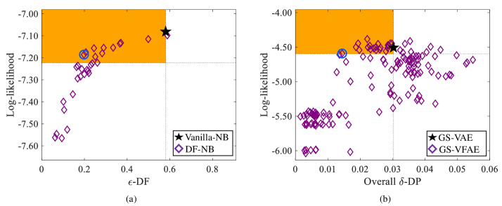
Figure 2: Selection strategy for fair models (purple diamonds): (a) DF-NB and (b) GS-VFAE. Black asterisk is the best typical model wrt log-likelihood: (a) Vanilla-NB and (b) GS-VAE. We select the best fair model (blue circle) wrt corresponding fairness metric from the orange area that satisfies our pre-defined rule.

Models	MI $\uparrow$	CH $\uparrow$	DB $\downarrow$	$\epsilon$-DF $\downarrow$	$\gamma$-SF $\downarrow$	$\delta$-DP $\downarrow$ (race)	$\delta$-DP $\downarrow$ (gender)	$\delta$-DP $\downarrow$ (nation)	$p\%$-Rule $\uparrow$ (race)	$p\%$-Rule $\uparrow$ (gender)	$p\%$-Rule $\uparrow$ (nation)
GS-VAE	0.132	1391.860	3.349	0.372	0.005	0.041	0.005	0.011	91.452	98.916	97.659
GS-VFAE	0.087	850.065	4.286	0.329	0.003	0.021	0.007	0.011	95.144	98.378	97.330
Vanilla-NB	0.137	1510.138	2.776	0.739	0.024	0.059	0.100	0.004	76.080	63.130	98.307
DF-NB	0.097	948.817	3.825	0.221	0.005	0.011	0.020	0.008	96.543	93.600	97.350

Table 1: Performance for clustering analysis on categorical variables in Adult dataset. Our DF-NB was the fairest model wrt $\epsilon$-DF along with several other fairness metrics, while our Vanilla-NB performed with highest clustering performances. Higher is better for measures with $\uparrow$, while lower is better for measures with $\downarrow$.

We validate and compare our models with two baseline models. For a typical baseline model that doesn’t take fairness into account, we consider the Gumbel-Softmax (GS) reparameterization-based VAE model for discrete latent variables (GS-VAE) [40]. As there is no existing work that enforces fairness in completely unsupervised setting for discrete latent variables, the work from Louizos et al. [21] is presumably the most relevant. They proposed an unsupervised fair VAE model $p_{\theta}(x|z,A)$ to factor out undesired information from the continuous latent variables $z$ by the marginally independent protected attributes $A$. We extend this model for discrete latent variables by GS reparameterization and use it as a fair baseline model (GS-VFAE) for our experiments.

We split the COMPAS into 60% train, 20% dev, and 20% test sets. For the Adult, we used the pre-specified train (32.56K) and test set (16.28K), and held-out 30% from the training data as the dev set. Finally, we held-out 10% from our larger data HHP as the test set, using the remainder for training, and further held-out 10% from the training data as the dev set. All the models were trained via the Adam optimizer [63] using PyTorch [77] on COMPAS, Adult and HHP datasets for a total of 50, 10 and 5 epochs, respectively. Finally. we performed grid search on the dev set to choose hyper-parameters, e.g., minibatch size, #neurons/hidden layer, learning rate, dropout, activation and random seed, from the same set of hyper-parameter values for all models (see appendix for the set of hyper-parameter values). Note that all experiments were conducted using only a CPU on an Intel Xeon E5-2623 V4 server with 64GB memory.

To evaluate the goodness of fit for all models, we compute average log-likelihood (LL) on held-out data. We also compute average mutual information (MI) [78, 79, 80] of $z$ over all observed variables to quantify how much meaningful information can be obtained from $z$. For clustering analysis, we measure commonly used metrics like Calinski-Harabasz (CH) score [81], where a higher score represents a model with better defined clusters, and Davies-Bouldin (DB) score [82], where a lower score represents a model with better separation between the clusters. In our SP model for criminal justice, we evaluate the predictive performance using LL, mean absolute error (MAE), mean squared error (MSE) and regression score ($R^{2}$) based on observed “jail time" in held-out data.

For evaluating from a fairness perspective, we compute $\epsilon$-DF which aims to ensure equitable treatment for all intersecting groups of all protected attributes. We also measure demographic parity ($\delta$-DP) [8] which ensures similar outcome probabilities for each protected group, $p\%$-Rule [19] which generalizes the $80\%$ rule of the U.S. employment law [59] for each protected group, and subgroup fairness ($\gamma$-SF) [12] which aims to prevent subset targeting in outcome variable by protecting all specified subgroups. To adapt $\gamma$-SF, $\delta$-DP and the $p\%$-Rule to multi-dimensional latent variables, we compute these metrics for each latent class, and report the worst case as the final metric, following Foulds et al. [13].

Models	MI $\uparrow$	CH $\uparrow$	DB $\downarrow$	$\epsilon$-DF $\downarrow$	$\gamma$-SF $\downarrow$	$\delta$-DP $\downarrow$ (age)	$\delta$-DP $\downarrow$ (gender)	$p\%$-Rule $\uparrow$ (age)	$p\%$-Rule $\uparrow$ (gender)
GS-VAE	0.069	913.774	4.221	1.385	0.045	0.335	0.048	32.311	83.524
GS-VFAE	0.061	793.340	4.523	1.123	0.042	0.320	0.040	39.108	84.329
Vanilla-GMM	0.106	1445.014	2.996	2.269	0.064	0.416	0.104	16.060	77.261
DF-GMM	0.044	597.302	4.183	0.275	0.021	0.078	0.049	84.338	89.964

Table 2: Performance for clustering analysis on continuous variables in HHP dataset. Our DF-GMM was the fairest model wrt $\epsilon$-DF along with most of the other fairness metrics, while our Vanilla-GMM performed with highest clustering performances. Higher is better for measures with $\uparrow$, while lower is better for measures with $\downarrow$.

Models	Measured in terms of observed “jail time"					Measured in terms of latent $z$
	LL $\uparrow$	MAE $\downarrow$	MSE $\downarrow$	$R^{2}$ $\uparrow$		$\epsilon$-DF $\downarrow$	$\gamma$-SF $\downarrow$	$\delta$-DP $\downarrow$ (race)	$\delta$-DP (gender) $\downarrow$	$p\%$-Rule $\uparrow$ (race)	$p\%$-Rule $\uparrow$ (gender)
Vanilla-SP	-1.301	0.578	0.757	0.274		1.744	0.035	0.143	0.093	40.844	43.929
DF-SP	-1.358	0.662	0.926	0.112		1.304	0.022	0.074	0.048	41.145	51.587

Table 3: Performance for our special purpose model on COMPAS dataset for criminal justice risk assessment. Predictive performances were measured wrt observed “jail time", while fairness were measured wrt $z$ that encodes risk of crime. Higher is better for measures with $\uparrow$, while lower is better for measures with $\downarrow$.

6.2 Fair Model Selection

Fair models divert the objective from only-the-ELBO to both ELBO and fairness, which can hurt the predictive performance of the models. Figure 2 demonstrates our strategy for a fair model selection on Adult dataset, which we followed for all experiments. We first obtained the best typical model (GS-VAE and our Vanilla-NB) based solely on LL for the dev set via grid search over the same set of hyper-parameter values (Black asterisk). Our fair model, DF-NB, was then assigned the same hyper-parameter values as the best Vanilla-NB, while the grid search was conducted over only the fairness trade-off parameter $\lambda$ (purple diamonds in Figure 2 (a)). As GS-VFAE does not provide any explicit trade-off parameter, we conducted the grid search over all hyper-parameter values (purple diamonds in Figure 2 (b)) like GS-VAE. Finally, we selected fair models that provide the best corresponding fairness metrics on the dev set, e.g., $\epsilon$-DF for DF-NB (blue circle in Figure 2 (a)) and overall $\delta$-DP for GS-VFAE (blue circle in Figure 2 (b)), allowing up to a slack tolerance, e.g., 2% degradation, in LL from the corresponding best typical model (orange area). Note that Louizos et al. [21] considered $\delta$-DP for a single protected attribute in their VFAE model. Since we consider multiple protected attributes, we selected the best GS-VFAE in terms of an overall $\delta$-DP metric, which is average of $\delta$-DP for each protected attribute. When deploying these methods in practice, the slack tolerance can be amended based on the stakeholders’ preferences.

6.3 Performance for Clustering

In this experiment, we evaluated the models on held-out test data for clustering analysis. For Adult data, models were trained on categorical observed variables like work classes, education levels, occupation types and income$\geq$50K or not, where we aimed to infer $z$ that represents whether an individual is “hard-working" or not. For our NB models, with the prior knowledge on the PDF of a logistic normal distribution, we set priors $\mathcal{N}(2,1)$ and $\mathcal{N}(-2,1)$ on $\mu_{z}$ to encode “hard-working” and not “hard-working,” respectively, and the same prior $\Gamma(1,2)$ on $\sigma_{z}$ for both cases. Table 1 shows that our Vanilla-NB outperformed all models in terms of clustering performance metrics like MI, CH and DB, while our DF-NB is the best fair model based on $\epsilon$-DF, as well as several other fairness metrics ($\delta$-DP (race) and p%-Rule race), with a small cost in performance.

In the HHP dataset, all models were trained on real-valued observations for hospitalized patients like estimation of mortality, drug counts, lab counts and so on, where we aimed to group the patients into 3 clusters that may represent short, medium and long length of stay in hospital so that we can help stakeholders to properly allocate healthcare resources. In our GMM models, we set informed priors on $\boldsymbol{\mu}_{z}$ using cluster centers from a k-means clustering method on train data and same prior $\mathcal{W}^{-1}(D+2,\mathbf{I})$ on $\boldsymbol{\Sigma}_{z}$ for all clusters. Table 2 shows that our DF-GMM is the fairest model based on almost all fairness metrics (5 out of 6) with a loss in clustering, while our Vanilla-GMM performed as best and worst model with respect to clustering metrics and fairness metrics, respectively.

6.4 Performance for Criminal Justice Risk Assessment

Models	$\epsilon$-DF $\downarrow$	$\gamma$-SF $\downarrow$	$\delta$-DP $\downarrow$ (race)	$\delta$-DP $\downarrow$ (gender)	$p\%$-Rule $\uparrow$ (race)	$p\%$-Rule $\uparrow$ (gender)
Vanilla-SP	0.085	0.005	0.027	0.003	94.323	99.364
DF-SP	0.100	0.006	0.015	0.019	96.873	96.063

Table 4: Fairness metrics measured on latent $u$ which encodes systems of oppression against individuals.

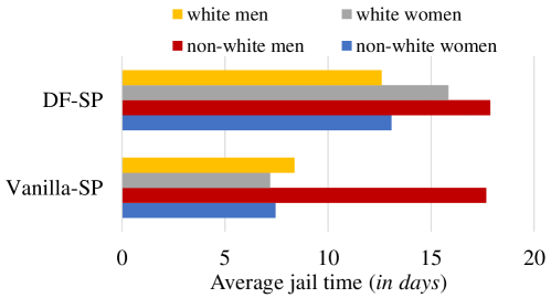
Figure 3: Generated average “jail time" in terms of intersecting protected groups for COMPAS data.

We investigate the performance of our SP models on the COMPAS system for criminal justice. Note that due to the well-known limitations with the COMPAS data [83], we caution against over-interpreting our experimental results. In Table 3, we show detailed results for our Vanilla-SP and DF-SP models. Note that we excluded the VAE-based baselines from this experiment since there is no straightforward way to extend them for the SP framework. According to the DAG presented in Figure 1 (c), we can evaluate the overall predictive performance in terms of “jail time". We measured fairness in terms of latent risk of crime $z$ since fairness intervention was applied to $z$. As expected, we found that Vanilla-SP performed better w.r.t predictive performance metrics, but worse w.r.t all fairness metrics. DF-SP mitigated these biases with a little sacrifice in predictive performances. Table 4 shows fairness measures on latent systems of oppression built into our society, where Vanilla-SP outperforms DF-SP model. This result is intuitive from the DAG. Since both risk of crime and systems of oppression can alter the “jail time,” improving fairness for one of them can increase disparity in the other.

We also looked into MI for COMPAS’s score (MI = 0.079), inferred risk of crime by Vanilla-SP (MI = 0.072) and by DF-SP (MI = 0.048) with actually occurred recidivism over a two-year period. Since COMPAS is a supervised learning-based system, it’s expected that COMPAS shows higher MI with the actual label, while our unsupervised Vanilla-SP and DF-SP performed with the comparable MI metric. Finally, in Figure 3, we visualized generated average “jail time" from our models in terms of all intersecting groups. We observe that Vanilla-SP reflected discrimination by predicting more “jail time" against a particular group, while DF-SP distributes similar “jail time" on average for all groups.

7 Conclusion

We have proposed an intersectional fair stochastic inference technique for discrete latent variable models. We have also presented a special-purpose model for mitigating societal biases from risk assessments in criminal justice. Our empirical results show the benefits of our approach in such sensitive tasks. In future work, we plan to work with criminologists to ensure its proper application and eventual deployment. We also plan to extend our custom latent variable modeling approach to tackle the case of learning fair algorithms with fully unobserved protected attributes.

Appendix A Related Work

Our fairness intervention technique in this work is inspired by intersectionality, the core theoretical framework underlying the third-wave feminist movement [50, 51]. Foulds et al. [13] proposed differential fairness which implements the principles of intersectionality with additional beneficial properties from a societal perspective regarding the law, privacy, and economics. While most of the fairness notions are defined for binary outcome and binary protected attribute, differential fairness conversely handles multiple outcomes and multiple protected attributes, simultaneously.

Much of the prior work that enforces fairness in variational inference [21, 28, 25, 27] using unsupervised probabilistic graphical models, e.g., VAE [29, 30], $\beta$-VAE [84], and FactorVAE [85], aims to learn fair representations of data using continuous latent variables for downstream classification tasks. Louizos et al. [21] also proposed a semi-supervised VAE model that encourages statistical independence between continuous latent variables and protected attributes using a maximum mean discrepancy (MMD) [86] penalty. Through the lens of representation learning, there are other recent advances in building fair classifiers using fair representations. Zemel et al. [9] proposed a neural network based supervised clustering model for learning fair representations that maps each data instance to a cluster, while the model ensures that each cluster gets assigned approximately equal proportions of data from each protected group. While this approach cannot leverage the representational power of a distributed representation, other work [20, 22, 23, 24] addressed this by developing joint framework using an autoencoder network to learn distributed representations along with an adversary network to penalize when protected attributes are predictable from representations and a classifier network to preserve utility-related information in the representations.

Appendix B Pseudo-code for Fair Variational Inference

Algorithm 1 Intersectional Fair Stochastic Variational Inference

Require: Train data $\mathbf{x}=\{x_{j}\}_{j=1}^{n}$

Require: Trade-off parameter $\lambda>0$

Require: Desired fairness $\epsilon_{0}$

Require: Constant step-size for expected counts $\rho_{t}$

Require: Constant step-size for optimization algorithm $\rho_{o}$

Require: Randomly initialized generative model’s parameters $\theta$, i.e., $\mu$ and $\sigma$

Require: Randomly initialized inference network’s parameters $\phi$, i.e., MLP’s weights and biases

Require: Fixed hyper-priors $p_{\alpha}(\theta)$

Require: Fixed prior $p_{\theta}(z)$

Output: Likelihood $p_{\theta}(x|z)$

Output: Variational Posterior $q_{\phi}(z|x)$

• For each epoch:

  • For each minibatch $m$:

    • Empirically estimate $\hat{N}_{z,s}=\sum_{x\in\mathbf{x}_{m}:A=s}\mathbf{z}_{m}$ and $\hat{N}_{s}$

    • Apply update: $N_{z,s}:=(1-\rho_{t})N_{z,s}+\rho_{t}\frac{n}{m}\hat{N}_{z,s}$

    • Apply update: $N_{s}:=(1-\rho_{t})N_{s}+\rho_{t}\frac{n}{m}\hat{N}_{s}$

    • Estimate $\epsilon(q_{\phi}(\mathbf{z}|\mathbf{x}),A)$ using $e^{-\epsilon}\leq\frac{N_{z,s_{i}}+\alpha}{N_{s_{i}}+K\alpha}\frac{N_{s_{j}}+K\alpha}{N_{z,s_{j}}+\alpha}\leq e^{\epsilon}$

    • Compute fairness penalty: $\mathcal{F}(\phi,A)=\text{max}(0,\epsilon(q_{\phi}(\mathbf{z}|\mathbf{x}),A)-\epsilon_{0})$

    • Apply update using stochastic gradient descent with $\rho_{o}$ via Equation 3 and 4:
          $\min_{\theta,\phi}\;-\frac{1}{m}\sum_{j=1}^{m}\mathcal{L}_{j}(\theta,\phi)+\lambda\mathcal{F}(\phi,A)$
          //in practice, Adam optimization via backpropagation and autodiff.

To further explain our methodology from Section 3 of the main paper, pseudo-code to our fair inference approach for discrete latent variable models is given in Algorithm 1.

Appendix C Hyper-parameter Tuning

Table 5: Set of hyper-parameter values for the grid search.

#neurons/hiddens layers for inference network	{[64, 64], [64, 32], [32, 16]}
minibatch size	{128, 256}
learning rate	{0.001, 0.002, 0.005}
dropout probability	{0.1, 0.25}
activation function	{ReLU, SoftPlus}
$l2$ regularization	{1$e$-3, 1$e$-4}
$\lambda$ for DF Models	{0.1, 0.2, 0.5, 0.8, 1.0, 2.0, 3.0, 4.0, 5.0, 6.0, 7.0, 8.0, 9.0, 1.5, 2.5, 3.5, 4.5, 5.5, 6.5, 7.5, 8.5, 9.5, 10.0, 15.0, 20.0, 25.0, 30.0, 50.0, 75.0, 100.0}

This additional section complements Section 6.1 in the main paper. Table 5 summarizes the set of hyper-parameter values used to perform the grid search on the dev set to choose the best model. First, the best typical models (Vanilla-NB, Vanilla-GMM, Vanilla-SP and GS-VAE) that do not account for fairness were selected based solely on LL for the dev set via grid search over minibatch sizes, #neurons/hidden layers, learning rates, dropout probabilities and activation functions, while we also considered random restarts to improve initialization with different random seeds for each combination of hyper-parameter values. The DF models (DF-NB, DF-GMM and DF-SP) were assigned the same hyper-parameter values, including selected seed, as the best corresponding vanilla models (Vanilla-NB, Vanilla-GMM and Vanilla-SP, respectively), while the grid search was conducted over only the fairness trade-off parameter $\lambda$. We then selected the best DF model using our pre-defined rule: select the DF model that provides the best $\epsilon$-DF metric on the dev set, allowing up to a slack tolerance in LL from the corresponding best vanilla model. There is no explicit fairness trade-off parameter, e.g., $\lambda$, in GS-VFAE model. Therefore, we conducted a full grid search for GS-VFAE model, similar to the typical models, and then chose the best model using the pre-defined rule: select the GS-VFAE model that provides the best overall $\delta$-DP metric on the dev set, allowing up to a slack tolerance in LL from the best GS-VAE model.

References

- Munoz et al. [2016] Cecilia Munoz, Megan Smith, and DJ Patil. Big data: A report on algorithmic systems. Opportunity, and Civil Rights, Executive Office of the President May, 2016.
- O’neil [2016] Cathy O’neil. Weapons of math destruction: How big data increases inequality and threatens democracy. Crown, 2016.
- Angwin et al. [2016] Julia Angwin, Jeff Larson, Surya Mattu, and Lauren Kirchner. Machine bias: There’s software used across the country to predict future criminals. and it’s biased against blacks. ProPublica, May, 23, 2016.
- Barocas and Selbst [2016] Solon Barocas and Andrew D Selbst. Big data’s disparate impact. Calif. L. Rev., 104:671, 2016.
- Bolukbasi et al. [2016] Tolga Bolukbasi, Kai-Wei Chang, James Y Zou, Venkatesh Saligrama, and Adam T Kalai. Man is to computer programmer as woman is to homemaker? debiasing word embeddings. Advances in neural information processing systems, 29, 2016.
- Campolo et al. [2017] Alex Campolo, Madelyn Rose Sanfilippo, Meredith Whittaker, and Kate Crawford. Ai now 2017 report. AI Now Institute at New York University, 2017.
- Noble [2018] Safiya Umoja Noble. Algorithms of oppression. In Algorithms of Oppression. New York University Press, 2018.
- Dwork et al. [2012] Cynthia Dwork, Moritz Hardt, Toniann Pitassi, Omer Reingold, and Richard Zemel. Fairness through awareness. In Proceedings of the 3rd innovations in theoretical computer science conference, pages 214–226. ACM, 2012.
- Zemel et al. [2013] Rich Zemel, Yu Wu, Kevin Swersky, Toni Pitassi, and Cynthia Dwork. Learning fair representations. In International conference on machine learning, pages 325–333. PMLR, 2013.
- Hardt et al. [2016] Moritz Hardt, Eric Price, and Nati Srebro. Equality of opportunity in supervised learning. Advances in neural information processing systems, 29, 2016.
- Kusner et al. [2017] Matt J Kusner, Joshua Loftus, Chris Russell, and Ricardo Silva. Counterfactual fairness. In Advances in Neural Information Processing Systems, 2017.
- Kearns et al. [2018] Michael Kearns, Seth Neel, Aaron Roth, and Zhiwei Steven Wu. Preventing fairness gerrymandering: Auditing and learning for subgroup fairness. In International Conference on Machine Learning, pages 2564–2572. PMLR, 2018.
- Foulds et al. [2020a] James R Foulds, Rashidul Islam, Kamrun Naher Keya, and Shimei Pan. An intersectional definition of fairness. In 2020 IEEE 36th International Conference on Data Engineering, pages 1918–1921. IEEE, 2020a.
- Keya et al. [2021] Kamrun Naher Keya, Rashidul Islam, Shimei Pan, Ian Stockwell, and James Foulds. Equitable allocation of healthcare resources with fair survival models. In Proceedings of the 2021 SIAM International Conference on Data Mining (SDM), pages 190–198. SIAM, 2021.
- Berk et al. [2018] Richard Berk, Hoda Heidari, Shahin Jabbari, Michael Kearns, and Aaron Roth. Fairness in criminal justice risk assessments: The state of the art. Sociological Methods & Research, page 0049124118782533, 2018.
- Foulds and Pan [2020] James R Foulds and Shimei Pan. Are parity-based notions of AI fairness desirable? Bulletin of the IEEE Technical Committee on Data Engineering, 43(4):51–73, 2020.
- Berk et al. [2017] Richard Berk, Hoda Heidari, Shahin Jabbari, Matthew Joseph, Michael Kearns, Jamie Morgenstern, Seth Neel, and Aaron Roth. A convex framework for fair regression. arXiv preprint arXiv:1706.02409, 2017.
- Islam et al. [2021] Rashidul Islam, Kamrun Naher Keya, Ziqian Zeng, Shimei Pan, and James Foulds. Debiasing career recommendations with neural fair collaborative filtering. In Proceedings of the Web Conference 2021, pages 3779–3790, 2021.
- Zafar et al. [2017] Muhammad Bilal Zafar, Isabel Valera, Manuel Gomez Rodriguez, and Krishna P Gummadi. Fairness beyond disparate treatment & disparate impact: Learning classification without disparate mistreatment. In Proceedings of the 26th international conference on world wide web, pages 1171–1180, 2017.
- Edwards and Storkey [2016] Harrison Edwards and Amos Storkey. Censoring representations with an adversary. In International Conference on Learning Representations, 2016.
- Louizos et al. [2016] Christos Louizos, Kevin Swersky, Yujia Li, Max Welling, and Richard S Zemel. The variational fair autoencoder. In International Conference on Learning Representations, 2016.
- Madras et al. [2018] David Madras, Elliot Creager, Toniann Pitassi, and Richard Zemel. Learning adversarially fair and transferable representations. In International Conference on Machine Learning, pages 3384–3393. PMLR, 2018.
- Zhao and Gordon [2019] Han Zhao and Geoff Gordon. Inherent tradeoffs in learning fair representations. Advances in neural information processing systems, 32, 2019.
- Zhao et al. [2020] Han Zhao, Amanda Coston, Tameem Adel, and Geoffrey J Gordon. Conditional learning of fair representations. In International Conference on Learning Representations, 2020.
- Creager et al. [2019] Elliot Creager, David Madras, Jörn-Henrik Jacobsen, Marissa Weis, Kevin Swersky, Toniann Pitassi, and Richard Zemel. Flexibly fair representation learning by disentanglement. In International Conference on Machine Learning, pages 1436–1445. PMLR, 2019.
- Bengio et al. [2013] Yoshua Bengio, Aaron Courville, and Pascal Vincent. Representation learning: A review and new perspectives. IEEE transactions on pattern analysis and machine intelligence, 35(8):1798–1828, 2013.
- Locatello et al. [2019] Francesco Locatello, Gabriele Abbati, Thomas Rainforth, Stefan Bauer, Bernhard Schölkopf, and Olivier Bachem. On the fairness of disentangled representations. In Advances in Neural Information Processing Systems, volume 32, pages 14611–14624, 2019.
- Song et al. [2019] Jiaming Song, Pratyusha Kalluri, Aditya Grover, Shengjia Zhao, and Stefano Ermon. Learning controllable fair representations. In The 22nd International Conference on Artificial Intelligence and Statistics, pages 2164–2173. PMLR, 2019.
- Kingma and Welling [2014] Diederik P. Kingma and Max Welling. Auto-encoding variational bayes. In International Conference on Learning Representations, 2014.
- Rezende et al. [2014] Danilo Jimenez Rezende, Shakir Mohamed, and Daan Wierstra. Stochastic backpropagation and approximate inference in deep generative models. In International conference on machine learning, pages 1278–1286. PMLR, 2014.
- Hoffman et al. [2013] Matthew D Hoffman, David M Blei, Chong Wang, and John Paisley. Stochastic variational inference. Journal of Machine Learning Research, 2013.
- Kingma et al. [2014] Durk P Kingma, Shakir Mohamed, Danilo Jimenez Rezende, and Max Welling. Semi-supervised learning with deep generative models. Advances in neural information processing systems, 27, 2014.
- Vahdat et al. [2018] Arash Vahdat, William Macready, Zhengbing Bian, Amir Khoshaman, and Evgeny Andriyash. Dvae++: Discrete variational autoencoders with overlapping transformations. In International Conference on Machine Learning, pages 5035–5044. PMLR, 2018.
- Malinowski et al. [2018] Mateusz Malinowski, Carl Doersch, Adam Santoro, and Peter Battaglia. Learning visual question answering by bootstrapping hard attention. In Proceedings of the European Conference on Computer Vision (ECCV), pages 3–20, 2018.
- Karim et al. [2021] Md Rezaul Karim, Oya Beyan, Achille Zappa, Ivan G Costa, Dietrich Rebholz-Schuhmann, Michael Cochez, and Stefan Decker. Deep learning-based clustering approaches for bioinformatics. Briefings in Bioinformatics, 22(1):393–415, 2021.
- Srivastava and Sutton [2017] Akash Srivastava and Charles Sutton. Autoencoding variational inference for topic models. In 5th International Conference on Learning Representations, 2017.
- Van Den Oord et al. [2017] Aaron Van Den Oord, Oriol Vinyals, et al. Neural discrete representation learning. Advances in neural information processing systems, 30, 2017.
- Shih and Ermon [2020] Andy Shih and Stefano Ermon. Probabilistic circuits for variational inference in discrete graphical models. Advances in Neural Information Processing Systems, 33:4635–4646, 2020.
- Vuffray et al. [2020] Marc Vuffray, Sidhant Misra, and Andrey Lokhov. Efficient learning of discrete graphical models. Advances in Neural Information Processing Systems, 33:13575–13585, 2020.
- Jang et al. [2016] Eric Jang, Shixiang Gu, and Ben Poole. Categorical reparameterization with gumbel-softmax. arXiv preprint arXiv:1611.01144, 2016.
- Maddison et al. [2016] Chris J Maddison, Andriy Mnih, and Yee Whye Teh. The concrete distribution: A continuous relaxation of discrete random variables. arXiv preprint arXiv:1611.00712, 2016.
- Chierichetti et al. [2017] Flavio Chierichetti, Ravi Kumar, Silvio Lattanzi, and Sergei Vassilvitskii. Fair clustering through fairlets. Advances in Neural Information Processing Systems, 30, 2017.
- Backurs et al. [2019] Arturs Backurs, Piotr Indyk, Krzysztof Onak, Baruch Schieber, Ali Vakilian, and Tal Wagner. Scalable fair clustering. In International Conference on Machine Learning, pages 405–413. PMLR, 2019.
- Madras et al. [2019] David Madras, Elliot Creager, Toniann Pitassi, and Richard Zemel. Fairness through causal awareness: Learning causal latent-variable models for biased data. In Proceedings of the conference on fairness, accountability, and transparency, pages 349–358, 2019.
- Harris [1999] David A Harris. The stories, the statistics, and the law: Why driving while black matters. Minnesota Law Review, 84:265, 1999.
- Harris [1996] David A Harris. Driving while black and all other traffic offenses: The supreme court and pretextual traffic stops. Journal of Criminal Law and Criminology, 87:544, 1996.
- Warren et al. [2006] Patricia Warren, Donald Tomaskovic-Devey, William Smith, Matthew Zingraff, and Marcinda Mason. Driving while black: Bias processes and racial disparity in police stops. Criminology, 44(3):709–738, 2006.
- Gelman et al. [2007] Andrew Gelman, Jeffrey Fagan, and Alex Kiss. An analysis of the new york city police department’s “stop-and-frisk” policy in the context of claims of racial bias. Journal of the American statistical association, 102(479):813–823, 2007.
- Carroll and Gonzalez [2014] Leo Carroll and M Lilliana Gonzalez. Out of place: Racial stereotypes and the ecology of frisks and searches following traffic stops. Journal of Research in Crime and Delinquency, 51(5):559–584, 2014.
- Crenshaw [1989] K. Crenshaw. Demarginalizing the intersection of race and sex: A black feminist critique of antidiscrimination doctrine, feminist theory and antiracist politics. U. Chi. Legal F., pages 139–167, 1989.
- Collins [2002] Patricia Hill Collins. Black feminist thought: Knowledge, consciousness, and the politics of empowerment. routledge, 2002.
- Dayan et al. [1995] Peter Dayan, Geoffrey E Hinton, Radford M Neal, and Richard S Zemel. The helmholtz machine. Neural computation, 7(5):889–904, 1995.
- Jaakkola and Jordan [1997] Tommi S Jaakkola and Michael I Jordan. A variational approach to bayesian logistic regression models and their extensions. In Sixth International Workshop on Artificial Intelligence and Statistics, pages 283–294. PMLR, 1997.
- Jordan et al. [1999] Michael I Jordan, Zoubin Ghahramani, Tommi S Jaakkola, and Lawrence K Saul. An introduction to variational methods for graphical models. Machine learning, 37(2):183–233, 1999.
- Gumbel [1954] Emil Julius Gumbel. Statistical theory of extreme values and some practical applications: a series of lectures, volume 33. US Government Printing Office, 1954.
- Maddison et al. [2014] Chris J Maddison, Daniel Tarlow, and Tom Minka. A* sampling. Advances in Neural Information Processing Systems, 27, 2014.
- Khemakhem et al. [2020] Ilyes Khemakhem, Diederik Kingma, Ricardo Monti, and Aapo Hyvarinen. Variational autoencoders and nonlinear ica: A unifying framework. In International Conference on Artificial Intelligence and Statistics, pages 2207–2217. PMLR, 2020.
- Zhou and Wei [2020] Ding Zhou and Xue-Xin Wei. Learning identifiable and interpretable latent models of high-dimensional neural activity using pi-vae. Advances in Neural Information Processing Systems, 33:7234–7247, 2020.
- Biddle [2006] Dan Biddle. Adverse impact and test validation: A practitioner’s guide to valid and defensible employment testing. Gower Publishing, Ltd., 2006.
- Foulds et al. [2020b] James R Foulds, Rashidul Islam, Kamrun Naher Keya, and Shimei Pan. Bayesian modeling of intersectional fairness: The variance of bias. In Proceedings of the 2020 SIAM International Conference on Data Mining, pages 424–432. SIAM, 2020b.
- Foulds et al. [2013] J.R. Foulds, L. Boyles, C. DuBois, P. Smyth, and M. Welling. Stochastic collapsed variational Bayesian inference for latent Dirichlet allocation. In Proceedings of the 19th ACM SIGKDD international conference on Knowledge discovery and data mining, pages 446–454, 2013.
- Islam and Foulds [2019] R. Islam and J.R. Foulds. Scalable collapsed inference for high-dimensional topic models. In Proceedings of the 2019 Conference of the North American Chapter of the Association for Computational Linguistics: Human Language Technologies, Volume 1 (Long and Short Papers), pages 2836–2845, 2019.
- Kingma and Ba [2015] Diederik P Kingma and Jimmy Lei Ba. Adam: A method for stochastic gradient descent. In ICLR: International Conference on Learning Representations, pages 1–15, 2015.
- LeCun et al. [2015] Yann LeCun, Yoshua Bengio, and Geoffrey Hinton. Deep learning. Nature, 521(7553):436–444, 2015.
- Paszke et al. [2017] Adam Paszke, Sam Gross, Soumith Chintala, Gregory Chanan, Edward Yang, Zachary DeVito, Zeming Lin, Alban Desmaison, Luca Antiga, and Adam Lerer. Automatic differentiation in pytorch. In Advances in Neural Information Processing Systems (Autodiff Workshop), 2017.
- Simoiu et al. [2017] C. Simoiu, S. Corbett-Davies, S. Goel, et al. The problem of infra-marginality in outcome tests for discrimination. The Annals of Applied Statistics, 11(3):1193–1216, 2017.
- Combahee River Collective [1978] Combahee River Collective. A black feminist statement. In Z. Eisenstein, editor, Capitalist Patriarchy and the Case for Socialist Feminism. Monthly Review Press, New York, 1978.
- Davis [2011] A.Y. Davis. Are prisons obsolete? Seven Stories Press, 2011.
- hooks [1981] b. hooks. Ain’t I a Woman: Black Women and Feminism. South End Press, 1981.
- Wald and Losen [2003] J. Wald and D.J. Losen. Defining and redirecting a school-to-prison pipeline. New Directions for Youth Development, 2003(99):9–15, 2003.
- Bowman et al. [2016] Samuel Bowman, Luke Vilnis, Oriol Vinyals, Andrew Dai, Rafal Jozefowicz, and Samy Bengio. Generating sentences from a continuous space. In Proceedings of The 20th SIGNLL Conference on Computational Natural Language Learning, pages 10–21, 2016.
- Kingma et al. [2016] Durk P Kingma, Tim Salimans, Rafal Jozefowicz, Xi Chen, Ilya Sutskever, and Max Welling. Improved variational inference with inverse autoregressive flow. Advances in neural information processing systems, 29, 2016.
- Semeniuta et al. [2017] Stanislau Semeniuta, Aliaksei Severyn, and Erhardt Barth. A hybrid convolutional variational autoencoder for text generation. In Proceedings of the 2017 Conference on Empirical Methods in Natural Language Processing, pages 627–637, 2017.
- Pelsmaeker and Aziz [2020] Tom Pelsmaeker and Wilker Aziz. Effective estimation of deep generative language models. In Proceedings of the 58th Annual Meeting of the Association for Computational Linguistics, pages 7220–7236, 2020.
- Ioffe and Szegedy [2015] Sergey Ioffe and Christian Szegedy. Batch normalization: Accelerating deep network training by reducing internal covariate shift. In International conference on machine learning, pages 448–456. PMLR, 2015.
- Alemi et al. [2018] Alexander Alemi, Ben Poole, Ian Fischer, Joshua Dillon, Rif A Saurous, and Kevin Murphy. Fixing a broken elbo. In International Conference on Machine Learning, pages 159–168. PMLR, 2018.
- Paszke et al. [2019] Adam Paszke, Sam Gross, Francisco Massa, Adam Lerer, James Bradbury, Gregory Chanan, Trevor Killeen, Zeming Lin, Natalia Gimelshein, Luca Antiga, et al. Pytorch: An imperative style, high-performance deep learning library. Advances in Neural Information Processing Systems, 32:8026–8037, 2019.
- Kozachenko and Leonenko [1987] Lyudmyla F Kozachenko and Nikolai N Leonenko. Sample estimate of the entropy of a random vector. Problemy Peredachi Informatsii, 23(2):9–16, 1987.
- Kraskov et al. [2004] Alexander Kraskov, Harald Stögbauer, and Peter Grassberger. Estimating mutual information. Physical review E, 69(6):066138, 2004.
- Ross [2014] Brian C Ross. Mutual information between discrete and continuous data sets. PloS one, 9(2):e87357, 2014.
- Caliński and Harabasz [1974] Tadeusz Caliński and Jerzy Harabasz. A dendrite method for cluster analysis. Communications in Statistics-theory and Methods, 3(1):1–27, 1974.
- Davies and Bouldin [1979] David L Davies and Donald W Bouldin. A cluster separation measure. IEEE transactions on pattern analysis and machine intelligence, pages 224–227, 1979.
- Bao et al. [2021] Michelle Bao, Angela Zhou, Samantha Zottola, Brian Brubach, Sarah Desmarais, Aaron Horowitz, Kristian Lum, and Suresh Venkatasubramanian. Itś COMPASlicated: The messy relationship between RAI datasets and algorithmic fairness benchmarks. In Proceedings of the Neural Information Processing Systems Track on Datasets and Benchmarks, 2021.
- Higgins et al. [2017] Irina Higgins, Loic Matthey, Arka Pal, Christopher Burgess, Xavier Glorot, Matthew Botvinick, Shakir Mohamed, and Alexander Lerchner. beta-vae: Learning basic visual concepts with a constrained variational framework. In International Conference on Learning Representations, 2017.
- Kim and Mnih [2018] Hyunjik Kim and Andriy Mnih. Disentangling by factorising. In International Conference on Machine Learning, pages 2649–2658. PMLR, 2018.
- Gretton et al. [2008] Arthur Gretton, Karsten M Borgwardt, Malte J Rasch, Bernhard Schölkopf, and Alexander Smola. A kernel method for the two-sample problem. Journal of Machine Learning Research, 1:1–10, 2008.