On error-based step size control for discontinuous Galerkin methods for compressible fluid dynamics

Abstract

We study temporal step size control of explicit Runge-Kutta methods for compressible computational fluid dynamics (CFD), including the Navier-Stokes equations and hyperbolic systems of conservation laws such as the Euler equations. We demonstrate that error-based approaches are convenient in a wide range of applications and compare them to more classical step size control based on a Courant-Friedrichs-Lewy (CFL) number. Our numerical examples show that error-based step size control is easy to use, robust, and efficient, e.g., for (initial) transient periods, complex geometries, nonlinear shock capturing approaches, and schemes that use nonlinear entropy projections. We demonstrate these properties for problems ranging from well-understood academic test cases to industrially relevant large-scale computations with two disjoint code bases, the open source Julia packages Trixi.jl with OrdinaryDiffEq.jl and the C/Fortran code SSDC based on PETSc.

AMS subject classification. 65L06, 65M20, 65M70, 76M10, 76M22, 76N99, 35L50

1 Introduction

Hyperbolic conservation laws are at the heart of many physical models in science and engineering, e.g., fluid dynamics describing the airflow around an airplane, acoustics, and space plasma modeling. Usually, the systems need to be solved numerically. A common approach is to apply the method of lines, i.e., to apply a spatial semidiscretization first and solve the resulting ordinary differential equation (ODE) numerically. For this task, explicit Runge-Kutta (RK) methods are among the most commonly used schemes because of their efficiency and parallel scalability [48, 53, 55].

Since demanding simulations require a significant amount of compute resources, there is a strong interest in developing efficient numerical methods. Here, efficiency can be measured by the required compute time, energy, and human time. The time- and energy-to-solution depend on the algorithms and their implementation as well as the hardware [93, 4, 41] and are often a focus of high performance computing (HPC) studies. The required human time depends on the robustness of the overall numerical method and the sensitivity with respect to parameters that may need to be tuned to ensure robustness and/or efficiency. In this article, we study error-based step size control for compressible flow problems to demonstrate that it is efficient in all three aspects.

We use entropy-dissipative semidiscretizations to ensure robustness [29, 31, 86, 83] but do not investigate specific implementation techniques discussed elsewhere [61, 33, 79]. Instead, we focus on step size control of time integration methods applied to ODEs resulting from spatial semidiscretizations of compressible flow problems. The goal is to adapt the time step size $\Delta t$ such that it is as big as possible while still satisfying accuracy and stability requirements. For explicit RK methods applied to (high-order) semidiscretizations, stability requirements are usually more restrictive. Thus, a commonly used approach is to adapt the time step size according to a Courant-Friedrichs-Lewy (CFL) number chosen by the user. This involves estimating local wave speeds and mesh spacing, which can be demanding for complex systems and curved high-order meshes in multiple space dimensions required in practice. The optimal CFL number depends on the space and time discretizations and possibly on the specific problem [84, 58, 14]. An alternative, widely used in the context of general-purpose ODE solvers, is an error-based step size control. There, a local error estimate is obtained from an embedded method and fed into a controller adapting the time step size according to user-specified tolerances. This approach has also been used successfully for partial differential equations [6, 94, 51, 76] but appears to be less-widely applied in the CFD community.

In this article, we systematically study error-based step size control for compressible CFD problems and compare it to CFL-based approaches. Specifically, we use the RK methods and controllers developed in [76] in two different software environments. Most of the examples use the open source packages OrdinaryDiffEq.jl [73] for ODE solvers and Trixi.jl [80, 85] for spatial semidiscretizations implemented in Julia [7]. Some large-scale, industrially-relevant CFD simulations are implemented in SSDC [67], which is built on top of the Portable and Extensible Toolkit for Scientific computing (PETSc) [3], its mesh topology abstraction (DMPLEX) [52], and its scalable ODE/DAE solver library [1]. All source code and instructions required to reproduce the numerical experiments using open source packages is available online in our reproducibility repository [81].

In the following, we briefly review RK methods and step size control techniques in Section 2. Afterwards, we study the robustness and sensitivity to user-supplied parameters under a change of mesh structure of both step size control approaches in Section 3. Section 4 focuses on the effect of nonlinear shock capturing schemes. In Section 5, we discuss the impact of an initial transient period, e.g., in the cold start of a simulation initialized with free stream values. Thereafter, we study step size control in the presence of a change of variables in Section 6. Next, we discuss the convenience of error-based step size control for exploratory research of new systems in Section 7. Finally, we summarize and discuss our findings in Section 8.

2 Runge-Kutta methods and step size control

We use the method of lines approach and first discretize a conservation law in space. In particular, we focus on spatial semidiscretizations using collocated discontinuous Galerkin methods (and related shock capturing schemes), see, e.g., [29, 31, 86, 83]. The resulting ordinary differential equation

$$\dfrac{\operatorname{d\!}{}}{\operatorname{d\!}{t}}u(t) =f(t,u(t)), t\in(0,T),$$ (2.1)

$$u(0) =u^{0},$$

is then solved using numerical time integration methods. Here, we use explicit Runge-Kutta methods with an embedded error estimator of the form [38, 12]

$$y_{i} =u^{n}+\Delta t_{n}\sum_{j=1}^{i-1}a_{ij}\,f(t_{n}+c_{j}\Delta t_{n},y_{j}),\qquad i\in\{1,\dots,s\},$$ (2.2)

$$u^{n+1} =u^{n}+\Delta t_{n}\sum_{i=1}^{s}b_{i}\,f(t_{n}+c_{i}\Delta t_{n},y_{i}),$$

$$\widehat{u}^{n+1} =u^{n}+\Delta t_{n}\sum_{i=1}^{s}\widehat{b}_{i}\,f(t_{n}+c_{i}\Delta t_{n},y_{i})+\widehat{b}_{s+1}f(t_{n+1},u^{n+1}).$$

Here, $u^{n+1}$ is the numerical solution of the main method, $\widehat{u}^{n+1}$ is the embedded methods solution used to obtain the local error estimate $u^{n+1}-\widehat{u}^{n+1}$, and $y_{i}$ are the stage values. RK methods are parameterized by their Butcher tableau

$$\begin{array}[]{c | c}c&A\\ \hline\cr&b^{T}\\ &\widehat{b}^{T}\end{array}$$ (2.3)

where $A=(a_{ij})_{i,j=1}^{s}\in\mathbb{R}^{s\times s}$ is strictly lower-triangular for explicit methods, $b,c\in\mathbb{R}^{s}$, and $\widehat{b}\in\mathbb{R}^{s+1}$. If $\widehat{b}_{s+1}\neq 0$, the RK pair (2.2) uses the so-called first-same-as-last (FSAL) idea to include the predicted value at the new time in the embedded error estimator [27]. This can increase the performance of the embedded method and comes at no additional cost if the step is accepted since $f(t_{n+1},u^{n+1})$ must be computed as the first stage of the next step anyway.

All methods considered in this article are applied in local extrapolation mode, i.e., a main method of order $q$ is coupled with an embedded error estimator of order $\widehat{q}=q-1$. Whenever possible, we make use of low-storage formats such as 3S*₊ [50, 76]. We use the same naming convention of RK methods as in [76], i.e., NAME$q$($\widehat{q}$)$s$ indicates an $s$-stage method of order $q$ with embedded error estimator of order $\widehat{q}$. This base name is followed by additional information on low-storage properties and a subscript “F” for FSAL methods.

2.1 Time integration loop and callbacks

We use implementations of the time integration methods available in OrdinaryDiffEq.jl [73] in Julia or PETSc/TS [1]. The basic steps for the time integration loop are given in Algorithm 1. At first, a preliminary time step is performed with the given RK method. If error-based step size control is activated, the embedded error estimator is also computed; it is used to update the time step size and determine whether the time step is rejected. After accepting a time step, callbacks are activated. We use these callback mechanisms for adaptive mesh refinement (AMR) and, if activated, CFL-based step size control.

Algorithm 1 High-level overview of a time integration step in the Julia package OrdinaryDiffEq.jl.

1. Compute preliminary time step update $u^{n+1}$ and the embedded solution $\widehat{u}^{n+1}$ if error-based step size control is activated using (2.2)

2. If error-based step size control is activated:

   • Let the step size controller update the time step size

   • If the time step is rejected, repeat step 1 with the updated time step size

3. Accept the new time step and update internal caches

4. Activate callbacks

5. Proceed to the next time step (i.e., increment the time step number $n$ and go to step 1)

A more detailed overview of the time integration loop is given below in Algorithm 2, discussed after introducing the step size control mechanisms.

2.2 CFL-based step size control

Explicit time integration methods for first-order hyperbolic conservation laws are subject to a CFL time step restriction of the form $\Delta t\leq C\Delta x/\lambda_{\mathrm{max}}$ [22]. However, it is non-trivial to provide sharp estimates of the terms in this restriction, e.g., an appropriate value for $\Delta x$ on curved meshes for high-order discontinuous Galerkin methods in multiple space dimensions. In general, CFL-based step size control requires user estimates of the maximal local wave speeds $\lambda_{\mathrm{max}}(u^{n}_{i})$ at the degree of freedom $u^{n}_{i}$ and the corresponding local mesh spacing $\Delta x_{i}$. Then, the time step is determined as

$$\Delta t_{n}=\nu\,\min_{i}\frac{\Delta x_{i}}{\lambda_{\mathrm{max}}(u^{n}_{i})},$$ (2.4)

where $\nu$ is the desired CFL number. For discontinuous Galerkin methods using polynomials of degree $p$ on (possibly) curved grids for the linear advection equation $\partial_{t}u+(a\cdot\partial_{x})u=0$, we follow [2, 76] and use the estimate

$$\frac{\Delta x_{i}}{\lambda_{\mathrm{max}}(u^{n}_{i})}=\frac{2}{p+1}\frac{J_{i}}{\sum_{j=1}^{d}|(J\partial_{x}\xi^{j})_{i}\cdot a|},$$ (2.5)

where $d$ is the number of spatial dimensions, $J_{i}$ the determinant of the grid Jacobian $\partial_{x}\xi$ at node $i$, $(J\partial_{x}\xi^{j})_{i}$ the contravariant basis vector in direction $j$ at node $i$ [54, Chapter 6], and $2$ is the size of the reference element. For nonlinear conservation laws, $a$ is replaced by appropriate estimates of the local wave speeds.

2.3 Error-based step size control

We perform error-based step size control based on controller ideas from digital signal processing [37, 36, 87, 88, 89]. In particular, we use PID controllers that select a new time step based on

$$\Delta t_{n+1}=\kappa\Bigl{(}\varepsilon_{n+1}^{\beta_{1}/k}\varepsilon_{n}^{\beta_{2}/k}\varepsilon_{n-1}^{\beta_{3}/k}\Bigr{)}\Delta t_{n},$$ (2.6)

where $k=\min(q,\widehat{q})+1$, $q$ is the order of the main method, and $\widehat{q}$ is the order of the embedded method. Because $\widehat{q}=q-1$ in our case, we have that $k=\widehat{q}+1=q$. Moreover, $\beta_{i}$ are the controller parameters, $\kappa$ is a step size limiter, and

$$\varepsilon_{n+1}=\frac{1}{w_{n+1}},\qquad w_{n+1}=\left(\frac{1}{m}\sum_{i=1}^{m}\left(\frac{u_{i}^{n+1}-\widehat{u}_{i}^{n+1}}{\tau_{a}+\tau_{r}\max\{|u_{i}^{n+1}|,|\widetilde{u}_{i}|\}}\right)^{2}\right)^{1/2},$$ (2.7)

where $m$ is the total number of degrees of freedom in $u$, and $\tau_{a},\tau_{r}$ are the absolute and relative error tolerances. In OrdinaryDiffEq.jl, $\widetilde{u}=u^{n}$ while PETSc uses $\widetilde{u}=\widehat{u}^{n+1}$. Unless stated otherwise, we use equal tolerances $\tau_{a}=\tau_{r}=\texttt{tol}$ and the default step size limiter $\kappa(a)=1+\arctan(a-1)$ [90].

The decision whether the step shall be accepted or rejected is determined by the size of the factor multiplying the time step size $\Delta t_{n}$ in (2.6). The default option used for all numerical experiments is to accept a step whenever the limited factor is at least $0.9^{2}$. Otherwise, the step is rejected and the time step size $\Delta t_{n}$ is set as the new predicted step size (2.6). Another common strategy is to decide whether a step should be rejected based only on the current local error estimate. Söderlind et al. [88, 90] argue why the approach we described here can be beneficial to reduce the amount of (unnecessary but expensive) step rejections.

To make the step size control fully automatic, we use the estimate of the initial step size implemented in OrdinaryDiffEq.jl from the algorithm described by Hairer et al. [38, p. 169]. $\varepsilon_{n}$ and $\varepsilon_{n-1}$ are initially set to one (for $n=0$).

A more detailed overview of the time integration loop including additional aspects about step size control and step rejections is shown in Algorithm 2. Parameters such as the threshold $0.9^{2}$ used to determine whether a step should be accepted or the limiting threshold $w_{\mathrm{min}}$ used in Algorithm 2 are based on recommendations in reference works such as [38, Section IV.2] and [12, Section 371]; we always use their default values and do not consider them as user-facing parameters that need to be chosen manually.

Algorithm 2 High-level overview of a time integration loop using explicit Runge-Kutta methods with embedded error estimator and PID controllers in OrdinaryDiffEq.jl and deviations in PETSc/TS.

1:Initialize time $t\leftarrow 0$, time step number $n\leftarrow 0$, and initial state $u^{0}$

2:Initialize PID controller with $\varepsilon_{0}\leftarrow 1$, $\varepsilon_{-1}\leftarrow 1$

3:Initialize $\Delta t_{0}=\widetilde{\Delta t}$ with a given value or the algorithm of [38, p. 169]

4:Initialize accept_step $\leftarrow$ false

5:while $t<T$ do

6:     if accept_step then $\triangleright$ callbacks can change accept_step

7:         accept_step $\leftarrow$ false $\triangleright$ prepare for the next step

8:         $t\leftarrow\widetilde{t}$

9:         $\Delta t_{n+1}\leftarrow\widetilde{\Delta t}$

10:         $n\leftarrow n+1$

11:     else

12:         $\Delta t_{n}\leftarrow\widetilde{\Delta t}$

13:     end if

14:     if $t+\Delta t_{n}>T$ then

15:         $\Delta t_{n}\leftarrow T-t$

16:     end if

17:     Compute $u^{n+1}$ and $\widehat{u}^{n+1}$ with time step $\Delta t_{n}$

18:     $w_{n+1}\leftarrow\sqrt{{\displaystyle\frac{1}{m}\sum_{i=1}^{m}}\left(\frac{u^{n+1}_{i}-\widehat{u}^{n+1}_{i}}{\tau_{a}+\tau_{r}\max\bigl{\{}\bigl{|}u^{n+1}_{i}\bigr{|},\bigl{|}\widetilde{u}_{i}\bigr{|}\bigr{\}}}\right)^{2}}$

19:     $\triangleright$ $\widetilde{u}=u^{n}$ in OrdinaryDiffEq.jl, $\widetilde{u}=\widehat{u}^{n+1}$ in PETSc

20:     $w_{n+1}\leftarrow\max\{w_{n+1},w_{\mathrm{min}}\}$

21:     $\triangleright$ $w_{\mathrm{min}}\approx$2.2\text{\times}{10}^{-16}$$ in OrdinaryDiffEq.jl, $=$1.0\text{\times}{10}^{-10}$$ in PETSc

22:     $\varepsilon_{n+1}\leftarrow 1/w_{n+1}$

23:     dt_factor $\leftarrow\kappa\Bigl{(}\varepsilon_{n+1}^{\beta_{1}/k}\varepsilon_{n}^{\beta_{2}/k}\varepsilon_{n-1}^{\beta_{3}/k}\Bigr{)}$ $\triangleright$ default $\kappa(a)=1+\arctan(a-1)$

24:     $\widetilde{\Delta t}\leftarrow$ dt_factor $\cdot\Delta t_{n}$

25:     if dt_factor $\geq$ accept_safety then $\triangleright$ default accept_safety $=0.81$

26:         accept_step $\leftarrow$ true

27:     else

28:         accept_step $\leftarrow$ false

29:     end if

30:     if accept_step then

31:         $\widetilde{t}\leftarrow t+\Delta t_{n}$

32:         if $\widetilde{t}\approx T$ then $\triangleright$ within 100 units in last place in OrdinaryDiffEq.jl

33:              $\widetilde{t}\leftarrow T$

34:         end if

35:         Apply callbacks $\triangleright$ AMR, CFL-based control in OrdinaryDiffEq.jl

36:     end if

37:end while

2.4 Importance of controller parameters

The RK pair (2.2) and the PID controller (2.6) must be developed together to obtain good results. In particular, semidiscretizations of conservation laws limited by stability should be integrated using a combination of RK pair and controller leading to stable step size control, based on the test equation [40], see also [39, Section IV.2] and [49]. This has been demonstrated for spectral element discretizations for compressible flows in [76]. In this article, we use the optimized controllers of [76].

2.5 Representative Runge-Kutta methods used in this article

There is a vast amount of literature on RK methods. Many schemes have been designed as general-purpose methods for low- or high-tolerance applications or even specifically for hyperbolic conservation laws. While we have performed numerical experiments with various schemes, we restrict this article to the following representative set of methods. First, we consider the general-purpose method

• BS3(2)3_F, the third-order, three-stage method of [8] (BS3() in OrdinaryDiffEq.jl, 3bs in PETSc)

This method has been shown to be among the most efficient — if not the most efficient — general purpose method for the CFD problems in which we are interested [76]. Next, we consider methods optimized for spectral element semidiscretizations of compressible CFD, namely

• RDPK3(2)5_F[3S*₊], the third-order, five-stage method of [76] (RDPK3SpFSAL35() in OrdinaryDiffEq.jl)

• RDPK4(3)9_F[3S*₊], the fourth-order, nine-stage method of [76] (RDPK3SpFSAL49() in OrdinaryDiffEq.jl)

Finally, we consider the strong stability preserving (SSP) method

• SSP3(2)4[3S*₊], the third-order, four-stage SSP method of [57] with embedded method of [21] and efficient implementation and step size controller of [76] (SSPRK43() in OrdinaryDiffEq.jl)

3 Robustness under change of mesh structure

Both CFL- and error-based step size control come with parameters that must be chosen by the user, either a CFL factor $\nu$ or a tolerance tol. However, the sensitivity with respect to these parameters differs significantly. The CFL factor $\nu$ influences the time step sizes — and thus the efficiency — linearly, while the tolerance tol has roughly a logarithmic influence. Thus, it is arguably easier to choose an appropriate tolerance than an optimal CFL factor.

Moreover, in the stability limited regime, it is often convenient to use error-based step size control since there is usually a range of tolerances resulting in the same number of right hand side (RHS) evaluations a manually optimized CFL-control could achieve at best. Furthermore, an optimal CFL factor $\nu$ depends on the mesh. Thus, it can vary when introducing curved coordinates compared to a uniform grid. This was already demonstrated for a 2D linear advection equation in [76, Section 3]. Here, we extend this demonstration to the nonlinear compressible Euler equations of an ideal gas in $d=3$ space dimensions given by

$$\partial_{t}\begin{pmatrix}\varrho\\ \varrho v_{i}\\ \varrho e\end{pmatrix}+\sum_{j=1}^{d}\partial_{x_{j}}\begin{pmatrix}\varrho v_{j}\\ \varrho v_{i}v_{j}+p\delta_{ij}\\ (\varrho e+p)v_{j}\end{pmatrix}=0,$$ (3.1)

where $\varrho$ is the density, $v$ the velocity, $\varrho e$ the total energy, and $p$ the pressure given by

$$p=(\gamma-1)\left(\varrho e-\frac{1}{2}\varrho v^{2}\right),$$ (3.2)

with the ratio of specific heats $\gamma=1.4$. Specifically, we consider the classical inviscid Taylor-Green vortex with initial data

$$\begin{gathered}\varrho^{0}=1,\;v_{1}^{0}=\sin(x_{1})\cos(x_{2})\cos(x_{3}),\;v_{2}^{0}=-\cos(x_{1})\sin(x_{2})\cos(x_{3}),\;v_{3}^{0}=0,\\ p^{0}=\frac{\varrho^{0}}{\mathrm{Ma}^{2}\gamma}+\varrho^{0}\frac{\cos(2x_{1})\cos(2x_{3})+2\cos(2x_{2})+2\cos(2x_{1})+\cos(2x_{2})\cos(2x_{3})}{16},\end{gathered}$$ (3.3)

where $\mathrm{Ma}=0.1$ is the Mach number. We consider the domain $[-\pi,\pi]^{3}$ with periodic boundary conditions and meshes with $8$ elements per coordinate direction. We apply entropy-dissipative discontinous Galerkin (DG) methods with polynomials of degree $p=3$ using a local Lax-Friedrichs flux at interfaces and the flux of [74, 75, 77] in the volume terms. We integrate the semidiscretizations in the time interval $[0,10]$.

We consider two meshes, a uniform Cartesian mesh and a curved mesh that heavily warps the Cartesian reference coordinates $(\xi,\eta,\zeta)\in[-1,1]^{3}$ to the desired mesh in physical coordinates $(x,y,z)$ with the mapping

$$\begin{gathered}\begin{aligned} y&=\eta+\frac{L_{y}}{8}\bigl{(}\cos(3\pi(\xi-c_{x})/L_{x})\cos(\pi(\eta-c_{y})/L_{y})\cos(\pi(\zeta-c_{z})/L_{z}\bigr{)},\\ x&=\xi+\frac{L_{x}}{8}\bigl{(}\cos(\pi(\xi-c_{x})/L_{x})\cos(4\pi(y-c_{y})/L_{y})\cos(\pi(\zeta-c_{z})/L_{z}\bigr{)},\\ z&=\zeta+\frac{L_{y}}{8}\bigl{(}\cos(\pi(x-c_{x})/L_{x})\cos(2\pi(y-c_{y})/L_{y})\cos(\pi(\zeta-c_{z})/L_{z}\bigr{)},\end{aligned}\\ L_{x}=L_{y}=L_{z}=2\pi,\quad c_{x}=c_{y}=c_{z}=0,\end{gathered}$$ (3.4)

that has been adapted from [17]. The curved mesh and the initial pressure are visualized in Figure 1.

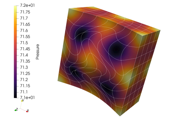
Figure 1: Initial pressure of the compressible Euler equations for the inviscid Taylor-Green vortex on a slice of the curved mesh.

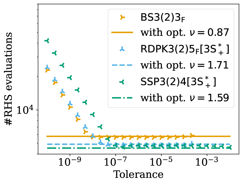
(a) Cartesian mesh.

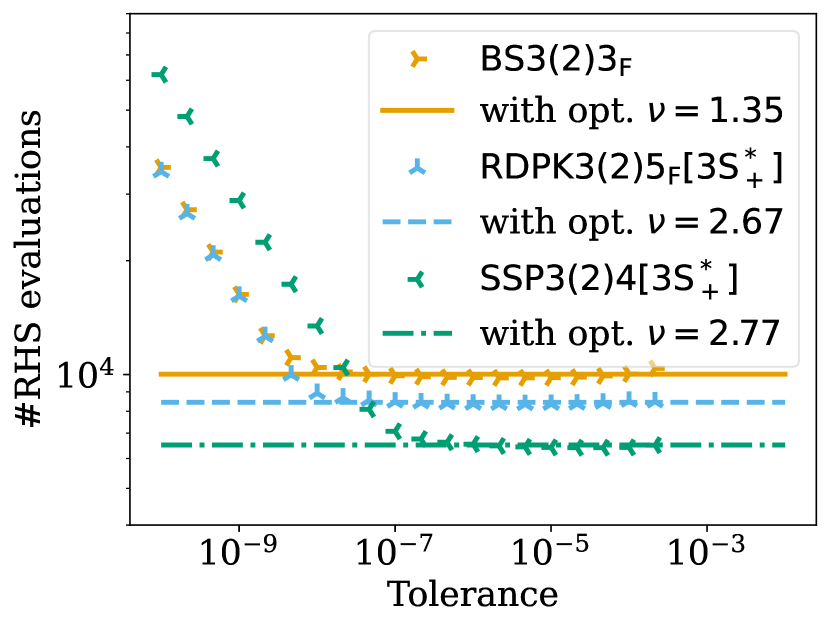
(b) Curved mesh.

Figure 2: Number of ODE RHS evaluations for representative RK methods using error-based (markers) and CFL-based (lines) step size control. The CFL factors were tuned manually to be as large as possible without crashing the simulation. Note that the optimized CFL factors are between $55\text{\,}\mathrm{\char 37\relax}$ and $74\text{\,}\mathrm{\char 37\relax}$ larger on the curved grid.

The required number of RHS evaluations for the selected, representative RK methods are shown in Figure 2, for CFL-based and error-based step size control. All RK methods show the same qualitative behavior on both grids. The step size for this problem is largely limited by stability, resulting in a range of tolerances yielding the optimal number of RHS evaluations one can also achieve by tuning the CFL factor manually (maximizing $\nu$ to three significant digits so that the simulations do not crash). This range of tolerances spans up to five orders of magnitude. For looser tolerances, the simulations may crash due to positivity issues, typically in the first few time step. Stricter tolerances let the controller detect an accuracy-limited regime and increase the number of RHS evaluations accordingly. This happens at looser tolerances for SSP3(2)4[3S*₊] than for the other methods since SSP3(2)4[3S*₊] is only optimized for the SSP coefficient while the other methods are also constructed to minimize the principal truncation error. Since all methods are of the same order of accuracy, the slope of the increasing number of RHS evaluations is the same.

However, there is a significant difference between CFL-based and error-based step size control when switching the mesh types. Indeed, the CFL factor can be increased between $55\text{\,}\mathrm{\char 37\relax}$ (for BS3(2)3_F) and $74\text{\,}\mathrm{\char 37\relax}$ (for SSP3(2)4[3S*₊]) on the curved mesh compared to the equivalent Cartesian mesh. In particular, choosing an optimized CFL factor from the uniform mesh results in the same amount of efficiency loss when the CFL factor is not tuned again manually from scratch. In contrast, basically the same range of tolerances can be used to get the optimal number of RHS evaluations on both grids for the error-based step size control.

4 Change of linear stability restrictions in nonlinear schemes

There are many shock capturing approaches for DG methods, e.g., artificial viscosity [72, 35], replacing DG elements by finite volume subcells [28, 91], modal filtering [63, 78], or specially constructed invariant domain preserving methods [71, 34, 59]. Here, we use the a priori convex blending of high-order DG elements with finite volume subcells described in [42].

4.1 Linear CFL restrictions

Shock capturing approaches in nonlinear schemes will typically change the linear CFL restriction on the time step for explicit time integration schemes. Here, we demonstrate this for some third-order schemes of the representative RK methods introduced in Section 2.5.

We consider the linear advection equation

$$\partial_{t}u(t,x)+\sum_{j=1}^{2}a^{j}\partial_{j}u(t,x)=0$$ (4.1)

in the domain $[-1,1]^{2}$ with periodic boundary conditions and velocity $a=(1,1)^{T}/\sqrt{2}$. We discretize the domain using $8^{2}$ uniform elements with polynomials of degree $p=3$ on Legendre-Gauss-Lobatto nodes. We choose a fixed blending parameter $\alpha=0.5$ in the shock capturing scheme of [42] with the standard discontinuous Galerkin collocation spectral element method (DGSEM), e.g., [54], and local Lax-Friedrichs flux for the finite volume subcells. We compute the spectra of the standard DGSEM scheme and the shock capturing scheme. Due to the fixed choice of the blending parameter, both semidiscretizations are linear and we compute their spectra numerically.

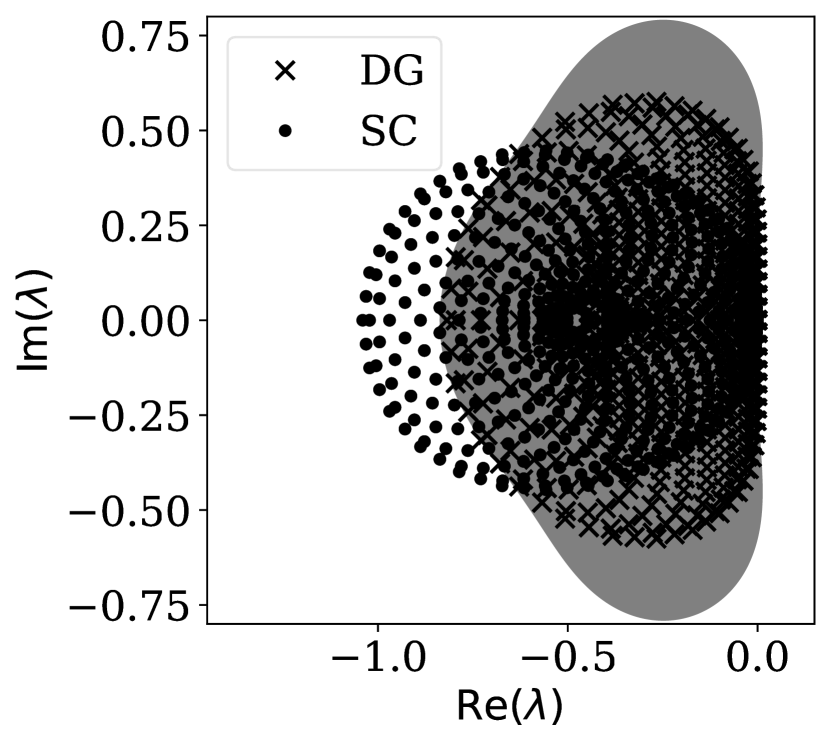
(a) BS3(2)3_F.

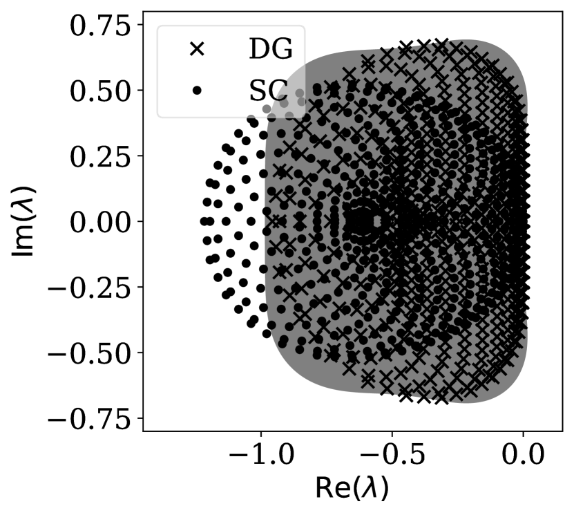
(b) RDPK3(2)5_F[3S*₊].

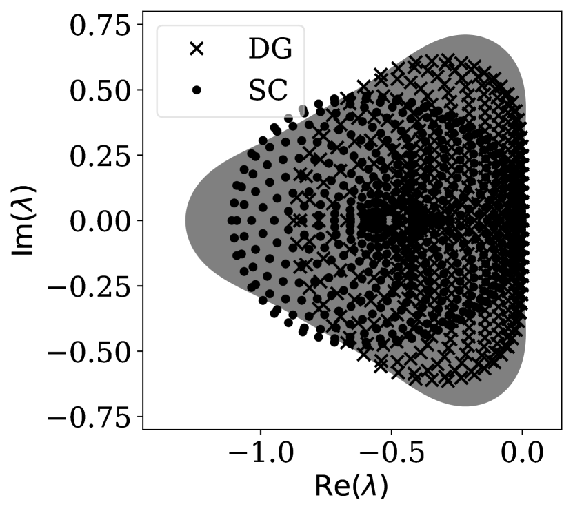
(c) SSP3(2)4[3S*₊].

Figure 3: Spectra of DGSEM and shock capturing (SC) semidiscretizations of the linear advection equation are embedded into the stability regions of some representative Runge-Kutta methods. The stability regions are scaled by the effective number of stages of the RK methods (taking the FSAL property into account). The spectra of the semidiscretizations are scaled by the maximal factor so that the standard DGSEM spectrum is in the region of absolute stability.

The spectra embedded into the stability regions of the representative RK methods are visualized in Figure 3. To make it easier to compare the RK methods, the stability regions are scaled by the effective number of RK stages, taking the FSAL property into account. The spectra of the semidiscretizations are scaled by the maximal factor so that the standard DGSEM spectrum is in the region of absolute stability of the RK method. Clearly, the (scaled) spectra of the shock capturing semidiscretizations are partially outside of the stability regions. Thus, one can expect a more restrictive CFL condition than for the standard DGSEM schemes.

These linear CFL restrictions predict an approximately one quarter bigger CFL number for standard DGSEM discretizations compared to the shock capturing variants for BS3(2)3_F and RDPK3(2)5_F[3S*₊]. For these time integration methods, the SC spectra extend significantly to the left-half of the complex plane outside of the stability regions, in particular near the negative real axis. The effect is qualitatively similar but quantitatively less pronounced for SSP3(2)4[3S*₊] (ca. $5\text{\,}\mathrm{\char 37\relax}$ instead of more than $20\text{\,}\mathrm{\char 37\relax}$).

4.2 Application to nonlinear magnetohydrodynamics: Orszag-Tang vortex

Next, we apply the representative time integration methods to entropy-dissipative semidiscretizations of the ideal generalized Lagrange multiplier (GLM) magnetohydrodynamics (MHD) equations [25, 9] for the Orszag-Tang vortex setup [66]. Specifically, we use the initial condition

$$\begin{gathered}\varrho^{0}=1,\quad v_{1}^{0}=-\sin(2\pi x_{2}),\quad v_{2}^{0}=\sin(2\pi x_{1}),\quad v_{3}^{0}=0,\quad p^{0}=1/\gamma,\\ B_{1}^{0}=-\sin(2\pi x_{2})/\gamma,\quad B_{2}^{0}=\sin(4\pi x_{1})/\gamma,\quad B_{3}^{0}=0,\quad\psi^{0}=0,\end{gathered}$$ (4.2)

in the domain $[0,1]^{2}$ with periodic boundary conditions, where $\varrho$ is the density, $v$ the velocity, $p$ the pressure, $B$ the magnetic field, and $\psi$ the Lagrange multiplier to control divergence errors. The ideal GLM-MHD equations with ratio of specific heats $\gamma=5/3$ and divergence cleaning speed $c_{h}=1$ are discretized on a uniform mesh with $2^{6}=64$ elements per coordinate direction and polynomials of degree $p=3$. We use the shock capturing method of [42] with the entropy-conservative numerical flux of [44] and a local Lax-Friedrichs flux at interfaces and for finite volume subcells, both with the nonconservative Powell source term. We use the product of density and pressure as the shock indicator variable with blending parameters $\alpha_{\mathrm{max}}=0.5$ and $\alpha_{\mathrm{min}}=0.001$.

(a) Density at $t\approx 0.11$.

(b) Density at $t\approx 0.19$.

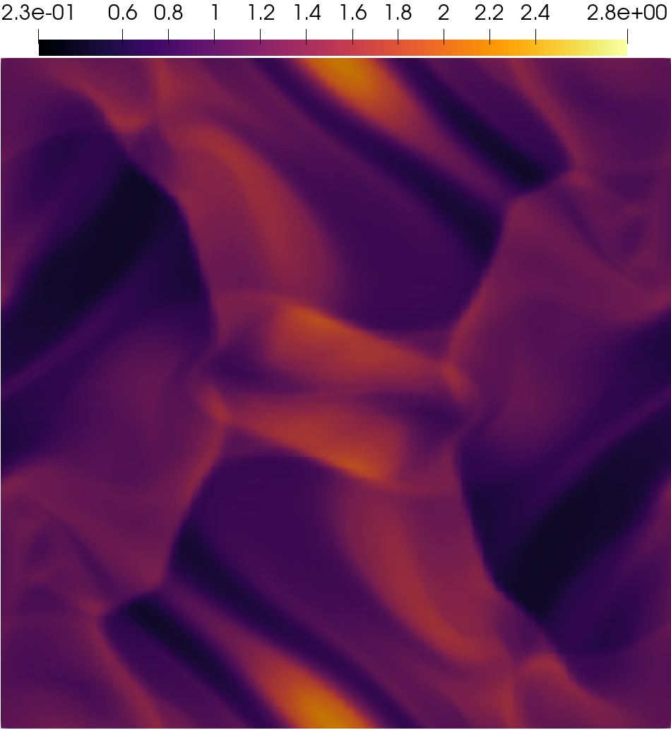
(c) Density at $t=0.50$.

(d) SCI at $t\approx 0.11$.

(e) SCI at $t\approx 0.19$.

(f) SCI at $t=0.50$.

Figure 4: Evolution of the density and the shock capturing indicator (SCI) computed using SSP3(2)4[3S*₊] and entropy-dissipative shock capturing semidiscretizations of the ideal GLM-MHD equations for the Orszag-Tang vortex.

As shown in Figure 4, the flow and its numerical approximation remain smooth in its initial phase. Between $t=0.1$ and $t=0.2$, the shock capturing indicator detects troubled cells and activates the finite volume shock capturing mechanism. At the final time, several shocklets are visible in the approximation.

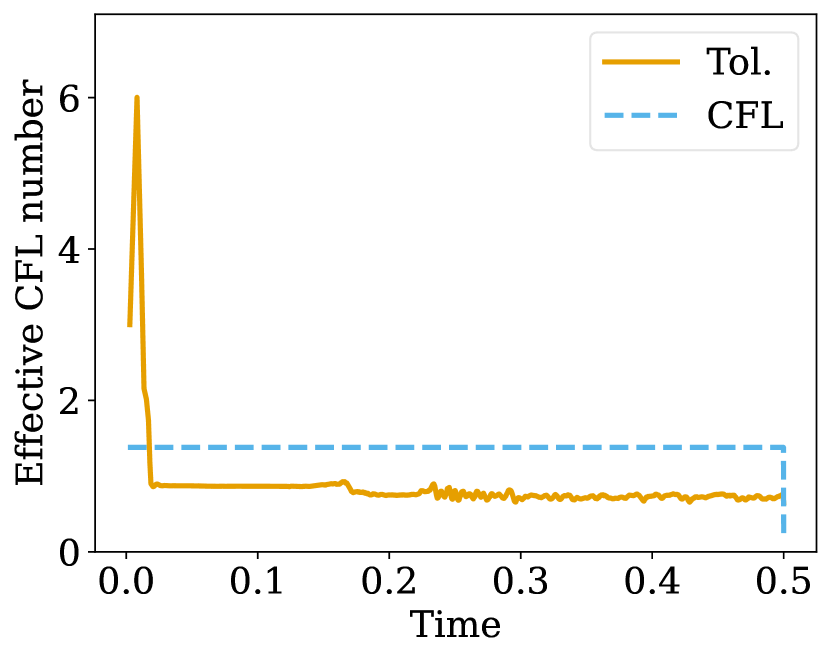
(a) BS3(2)3_F.

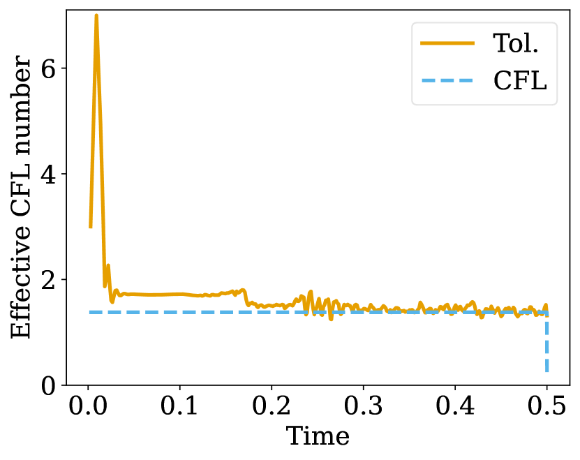
(b) RDPK3(2)5_F[3S*₊].

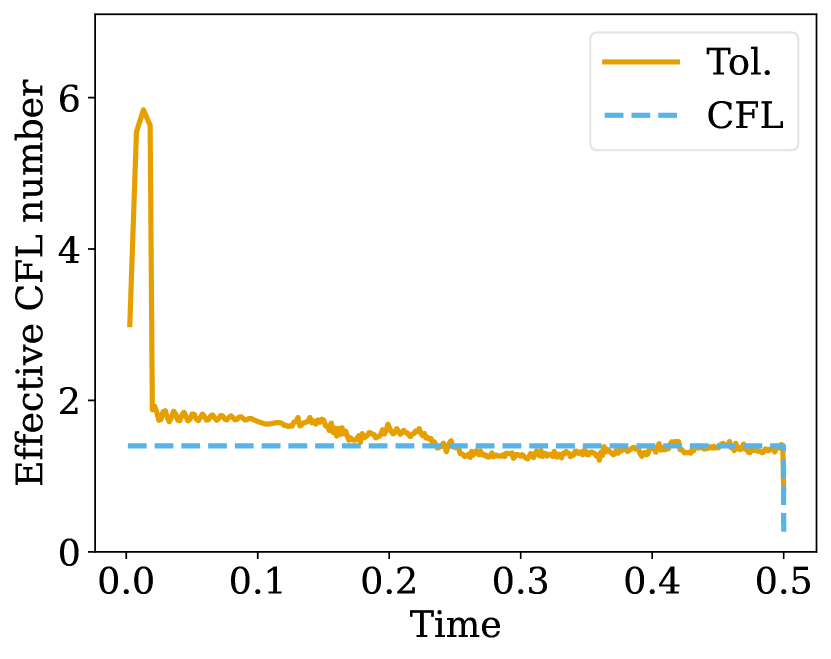
(c) SSP3(2)4[3S*₊].

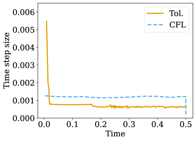
(d) BS3(2)3_F.

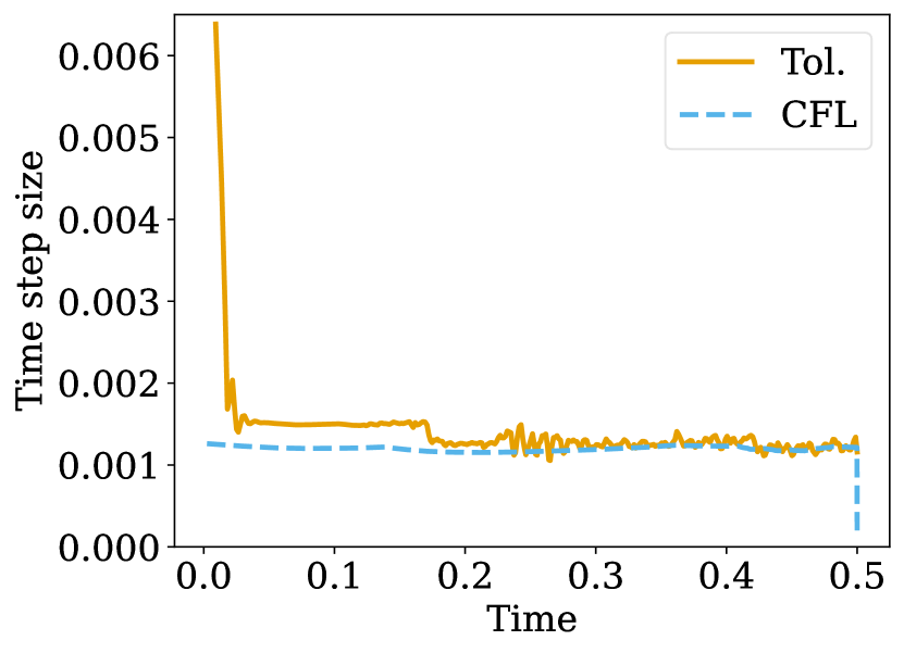
(e) RDPK3(2)5_F[3S*₊].

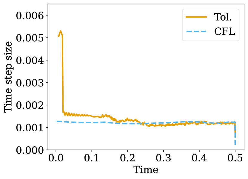
(f) SSP3(2)4[3S*₊].

Figure 5: Effective CFL numbers (first row) and time step sizes (second row) of some representative RK methods applied to entropy-dissipative shock capturing semidiscretizations of the ideal GLM-MHD equations for the Orszag-Tang vortex.

We recorded the time step sizes and effective CFL numbers, i.e., the CFL factor computed a posteriori based on the time step size chosen by the error-based step size controller, after every accepted time step for some representative RK methods. The tolerance is set to $\texttt{tol}=10^{-4}$ in all cases with error-based step size control. For CFL-based step size control, we bisected the maximal CFL number without blow-up to three significant digits. The results are shown in Figure 5. Clearly, the time step size of the CFL-based approaches does not vary significantly in time. Thus, the estimated CFL restriction are nearly constant. However, the nonlinear schemes activate shock capturing mechanisms between $t=0.1$ and $t=0.2$. Thus, the estimated linear CFL restriction should become more severe as discussed in Section 4.1. This can be observed also for error-based step size control; all RK methods use larger time steps initially until the shock capturing part is activated. Then, error-based step size control yields approximately the maximal step size also used by CFL-based step size control with manually tuned CFL number. In particular, the initial time step size is approximately one quarter bigger with error-based step size control (after the controller has adapted the time step size from the automated initial guess). During the full simulation, error-based step size control results in the following performance improvements based on the number of function evaluations (see also Table 1): $13\text{\,}\mathrm{\char 37\relax}$ for BS3(2)3_F, $11\text{\,}\mathrm{\char 37\relax}$ for RDPK3(2)5_F[3S*₊], and $6\text{\,}\mathrm{\char 37\relax}$ for SSP3(2)4[3S*₊].

While the quantitative numbers for BS3(2)3_F and RDPK3(2)5_F[3S*₊] fit very well to the linear analysis, one could expect that the initial advantage of SSP3(2)4[3S*₊] with error-based step size control should be smaller, since the stability region is less optimal for high-order DGSEM and relatively better suited for low-order shock capturing methods. First, we do not necessarily expect that such a linear analysis is quantitatively correct for general nonlinear problems, although it was shown to behave very well in applications [70]. Second, the shock capturing mechanism also changes the behavior of the ODE RHS, usually reducing the smoothness of the spatially discrete system, which also affects step size control.

Table 1: Performance of representative RK methods with default error-based and manually tuned CFL-based step size controllers: Number of function evaluations (#FE), accepted steps (#A), and rejected steps (#R) for the Orszag-Tang vortex with entropy-dissipative shock capturing semidiscretizations.

Scheme	$\beta$	tol/$\nu$	#FE	#A	#R
BS3(2)3F	$(0.60,-0.20,0.00)$	$\texttt{tol}=10^{-4}$	$2187$	$724$	$4$
		$\nu=0.69$	$2506$	$835$
RDPK3(2)5F[3S*+]	$(0.70,-0.23,0.00)$	$\texttt{tol}=10^{-4}$	$1863$	$368$	$4$
		$\nu=1.38$	$2091$	$418$
SSP3(2)4[3S*+]	$(0.55,-0.27,0.05)$	$\texttt{tol}=10^{-4}$	$1550$	$384$	$3$
		$\nu=1.40$	$1648$	$412$

As expected, the method RDPK3(2)5_F[3S*₊] optimized for spectral element discretizations performs better than the general-purpose method BS3(2)3_F and uses $15\text{\,}\mathrm{\char 37\relax}$ less function evaluations (with error-based step size control). For this problem with a significant amount of shock capturing, SSP3(2)4[3S*₊] with error-based step size performs even better and uses additionally $16\text{\,}\mathrm{\char 37\relax}$ less function evaluations than RDPK3(2)5_F[3S*₊].

In summary, the results of this section demonstrate that error-based step size control can react robustly and efficiently to varying linear CFL restrictions in nonlinear schemes. In particular, they usually require less parameter tuning while still achieving optimal performance. For this problem with a significant amount of shock capturing mechanisms, the strong stability preserving method SSP3(2)4[3S*₊] performs well.

5 Initial transient period: cold start of a simulation

When performing a cold start of a demanding CFD simulation, e.g., by initializing the flow around objects with free stream values, the initial transient period often requires smaller time steps than the fully developed simulation. For demanding simulations with positivity issues for high-order spatial schemes used in this section, we apply SSP time integration methods.

5.1 Double Mach reflection of a strong shock

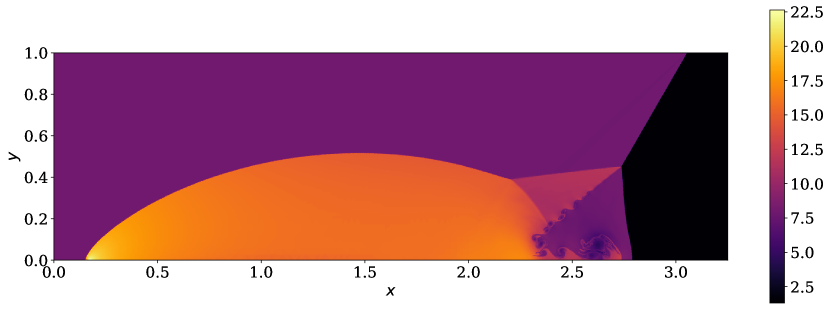
(a) Density.

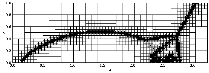
(b) Mesh.

Figure 6: Density and mesh at the final time of the simulation of the Woodward-Colella double Mach reflection using SSP3(2)4[3S*₊] applied to entropy-dissipative shock capturing semidiscretizations with positivity-preserving limiters and adaptive mesh refinement.

First, we consider the double Mach reflection of Woodward and Colella [97]. We set up an initial grid with 80 uniform elements that is adaptively refined during the simulation using p4est [11]. We use the shock capturing approach of [42] with DG elements using polynomials of degree $p=4$ and the entropy-conservative numerical flux of [74, 75, 77] in the volume terms and a local Lax-Friedrichs flux at interfaces and finite volume subcells. AMR is triggered every two time steps and the positivity-preserving limiter of [99] for density and pressure is applied after every Runge-Kutta stage. We apply SSP3(2)4[3S*₊] to integrate the system in time $t\in[0,0.2]$. The complete setup can be found in the reproducibility repository [81]. Figure 6 shows the density and the mesh at the final time.

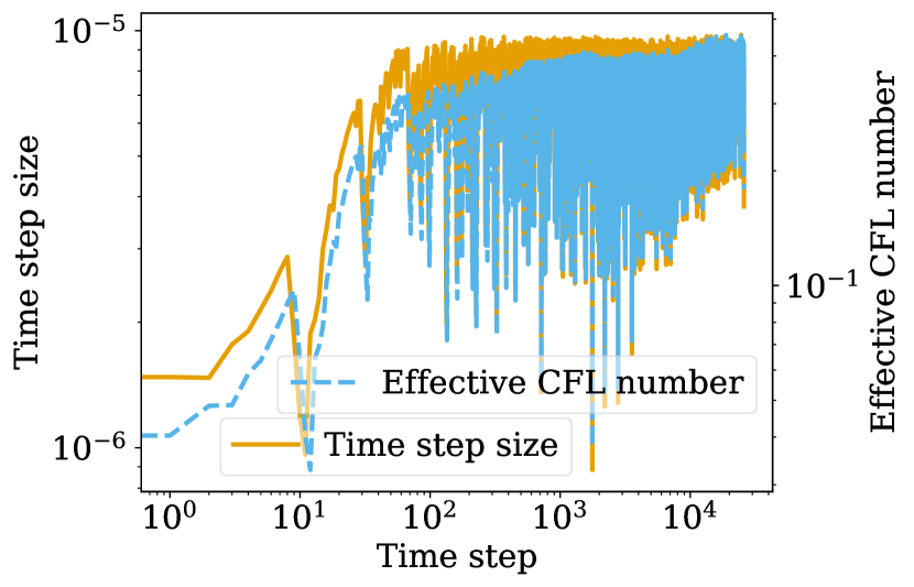
(a) Dependence on time step number.

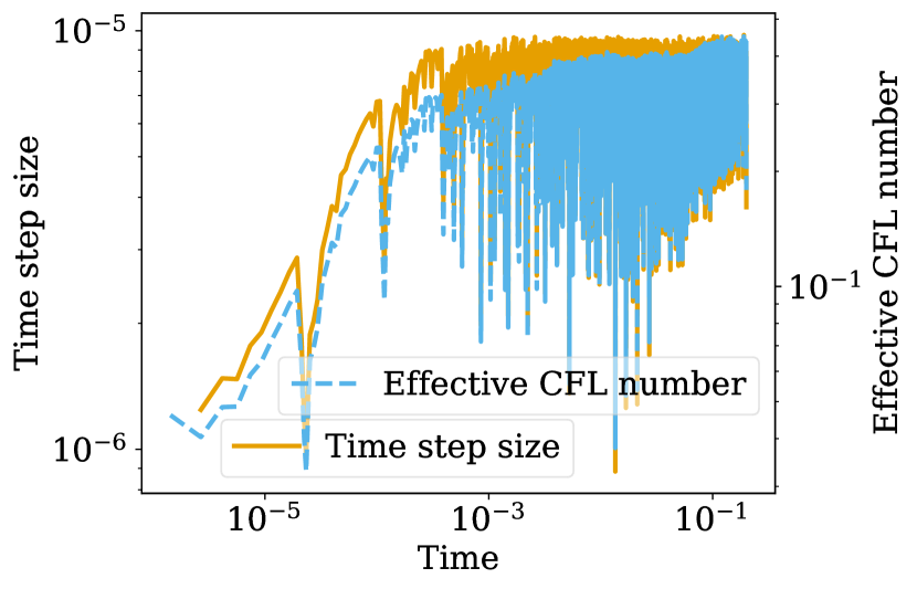
(b) Dependence on time.

Figure 7: Time step sizes and effective CFL numbers of SSP3(2)4[3S*₊] applied to entropy-dissipative shock capturing semidiscretizations with positivity-preserving limiters and adaptive mesh refinement for the double Mach reflection problem.

Figure 7 shows the evolution of the time step sizes and the effective CFL number. There is an initial transient period of ca. 100 time steps where both the time step size and the effective CFL number are much smaller than in the remaining simulation. This small initial step size is selected by the automatic detection algorithm and the error-based step size control, no manual intervention is necessary. The same simulation setup run with CFL-based step size control crashes in the first few time steps, even with a small CFL number of $\nu=0.01$. The initial transient period can be captured with even smaller CFL numbers, but running the simulation afterwards in a reasonable amount of time required adapting the CFL factor. In contrast, error-based step size control can be used with the same parameters throughout the simulation.

5.2 Astrophysical Mach 2000 jet

Next, we consider a simulation of an astrophysical Mach 2000 jet using the ideal compressible Euler equations with ratio of specific heat $\gamma=5/3$ based on the setup of [60]. Specifically, we use the initial condition

$$\varrho^{0}=0.5,\quad v_{1}^{0}=0,\quad v_{2}^{0}=0,\quad p^{0}=0.4172$$ (5.1)

in the domain $[-0.5,0.5]$ equipped with periodic boundary conditions in $y$-direction and Dirichlet boundary conditions using the initial data in the $x$-direction except for $t>0$, $x=-0.5$, and $y\in[-0.05,0.05]$, where we use boundary data (denoted by a superscript $b$)

$$\varrho^{b}=5,\quad v_{1}^{b}=800,\quad v_{2}^{b}=0,\quad p^{b}=0.4172.$$ (5.2)

We use an initially uniform mesh with $64$ elements per coordinate direction and polynomials of degree $p=3$. We use the shock capturing approach of [42] with the entropy-conservative numerical flux of [74, 75, 77] in the volume terms and a local Lax-Friedrichs flux at interfaces and finite volume subcells. After every time step, we apply adaptive mesh refinement. Moreover, we apply the positivity-preserving limiter of [99] for density and pressure after every Runge-Kutta stage. We integrate the semidiscrete system in time using SSP3(2)4[3S*₊] for $t\in[0,10^{-3}]$. The complete setup can be found in the reproducibility repository [81].

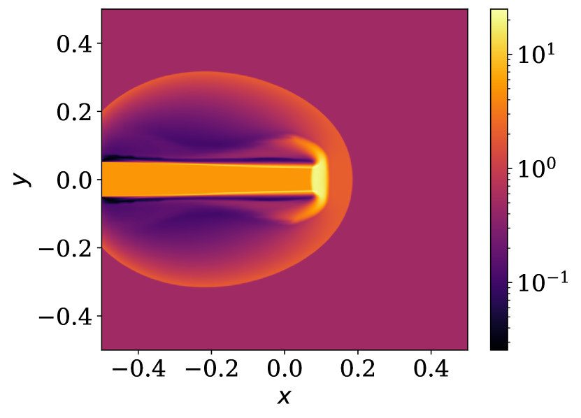
(a) Density.

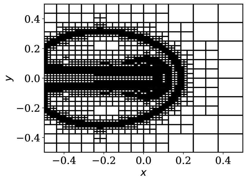
(b) Mesh.

Figure 8: Density and mesh at the final time of the simulation of an astrophysical Mach 2000 jet using SSP3(2)4[3S*₊] applied to entropy-dissipative shock capturing semidiscretizations with positivity-preserving limiters and adaptive mesh refinement.

Figure 8 shows a snapshot of the numerical solution and the adapted grid at the final time $t=10^{-3}$. While the initial condition is given by uniform free stream values, the boundary condition (5.2) changes the numerical approximation rapidly in time. Consequently, the mesh is refined over time and adapts to the solution structures.

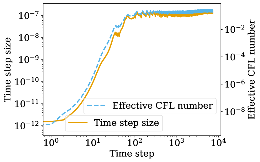
(a) Dependence on time step number.

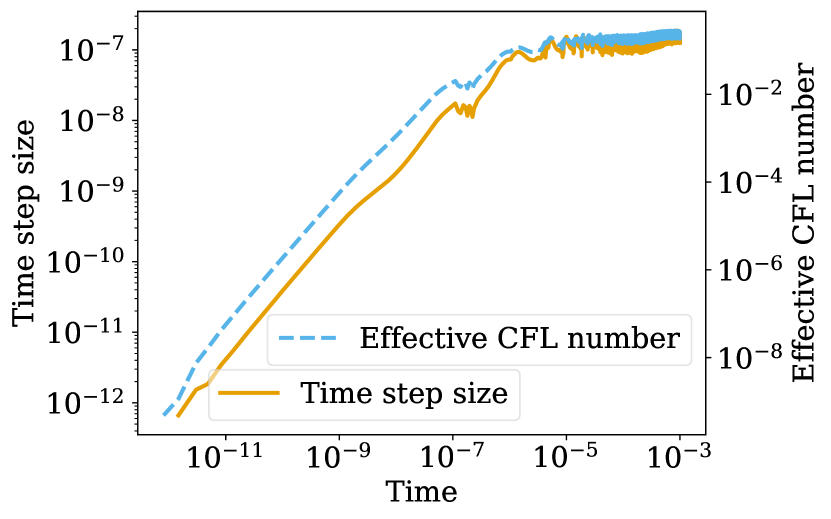
(b) Dependence on time.

Figure 9: Time step sizes and effective CFL numbers of SSP3(2)4[3S*₊] applied to entropy-dissipative shock capturing semidiscretizations with positivity-preserving limiters and adaptive mesh refinement for the astrophysical Mach 2000 jet.

Figure 9 shows the evolution of the time step for this demanding simulation. The initial time step must be very small — of the order $\Delta t\approx 10^{-12}$ — to allow the simulation to run. For this setup, we set $\Delta t=10^{-12}$ initially; other choices are also possible and are adapted to similar values automatically by the controller, but the fully automatic initial guess is not sufficient in this case.

The initial transient period lasts for ca. 100 time steps where the error-based step size controller increases the time step size gradually. Afterwards, the time step size plateaus. Handling such an initial transient period is difficult for standard CFL-based step size controllers. Initially, a CFL factor of $\nu\approx 10^{-9}$ is required; $\nu=10^{-8}$ results in a blow-up of the simulation. One could implement a more complicated CFL-based controller adapting the CFL factor in the initial transient period or restart the simulation after ca. 100 time steps with a larger CFL factor. However, no such additional techniques are required for error-based step size control, making it easier to use in this case.

5.3 Delta wing

The next test case setup approximates the solution of the compressible Navier-Stokes equations. We consider an industrially relevant simulation of a $65\mathrm{°}$ swept delta wing at a Mach number $\mathrm{Ma}=0.9$, a Reynolds number $\mathrm{Re}=10^{6}$ (based on the mean aerodynamic chord), and setting the angle of attack to $\mathrm{AoA}=$$$. The geometry was proposed by Hummel and Redeker [47] for the Second International Vortex Flow Experiment (VFE-2) and manufactured based on a NASA wing geometry that served as reference configuration [20]. We consider the flow past the leading edge configuration with a medium radius leading edge $r_{LE}/\bar{c}=0.0015$, where $\bar{c}=$0.653\text{\,}\mathrm{m}$$. The delta wing has a mean aerodynamic chord of $\ell=$0.667\text{\,}\mathrm{m}$$, a root chord length of $c_{r}=1.47\ell$, and a wing span of $b=1.37\ell$. The sting present in the wind tunnel testing is kept downstream as part of the geometry up to the position $x_{1}/c_{r}=1.758$, where the $x_{1}$ Cartesian coordinate points in the streamwise direction as shown in the left part of Figure 10.

For this test, we use the $hp$-adaptive entropy stable solver SSDC [67], which is able to deliver numerical results in good agreement with experimental data. Entropy stable adiabatic no-slip wall boundary conditions [23] are applied to the wing and sting surfaces, whereas freestream far-field boundary conditions are applied at the inlet and outlet planes. Due to the symmetry of the problem in the span-wise direction, half span of the flow is modeled through a symmetry boundary condition. On the rest of the boundary planes, entropy stable inviscid wall boundary conditions [69] are prescribed. The grid consists of $\approx 9.2\times 10^{4}$ hexahedral elements. It is subdivided into three blocks, as shown in the right part of Figure 10, with each block corresponding to a different solution polynomial degree $p$. In particular, we use $p=2$ in the far-field region, $p=5$ in the region surrounding the delta wing and its support, and $p=3$ elsewhere. Given the degree of the solution and the number of elements in each block, the total number of degrees of freedom (DOFs) is $\approx 1.435\times 10^{7}$.

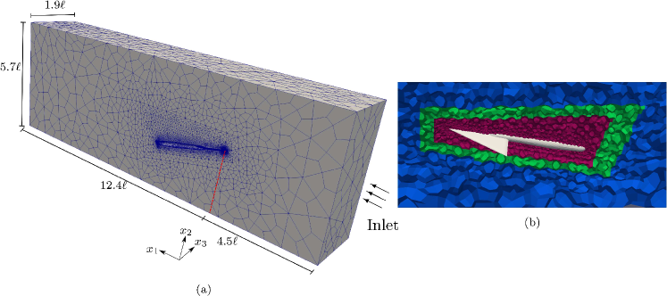
Figure 10: Solution polynomial degree distribution, $p$, computational domain and boundary mesh elements for the $65\mathrm{°}$ swept delta wing test case [67].

The flow around a delta wing is peculiar. When the angle of attack exceeds $7\mathrm{°}$, typically, flow separation occurs at the leading edge. The roll up of the leading-edge vortices induces low pressure on the upper surface of the wing and enhances the lift. Figure 11 shows the instantaneous pressure coefficient distribution and streamlines colored by the velocity magnitude at $t=0.05$.

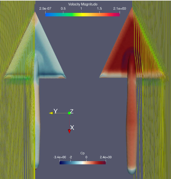
Figure 11: Instantaneous pressure coefficient distribution and streamlines colored by the velocity magnitude at $t=0.05$ for the $65\mathrm{°}$ swept delta wing test case [67] (left: top view, right: bottom view).

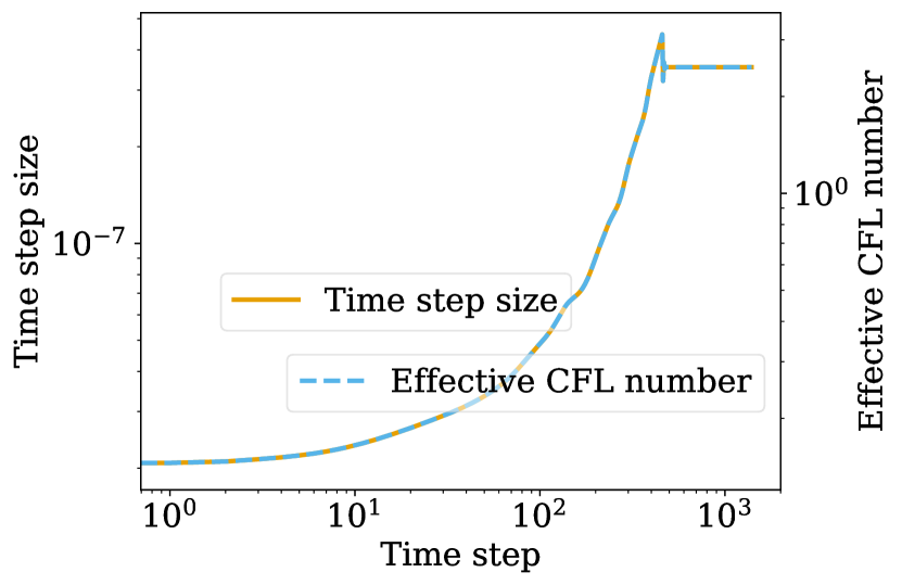
(a) BS3(2)3_F (time step number).

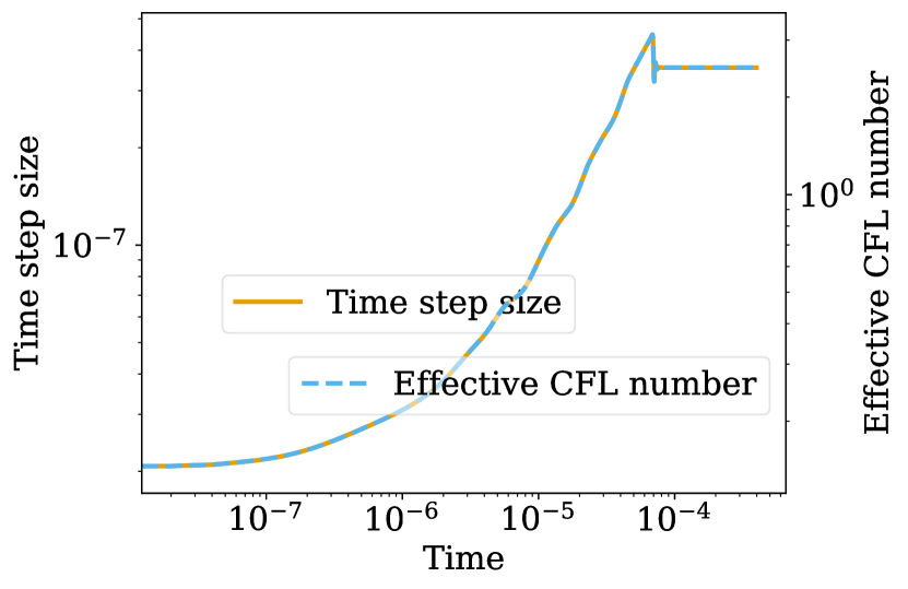
(b) BS3(2)3_F (physical time).

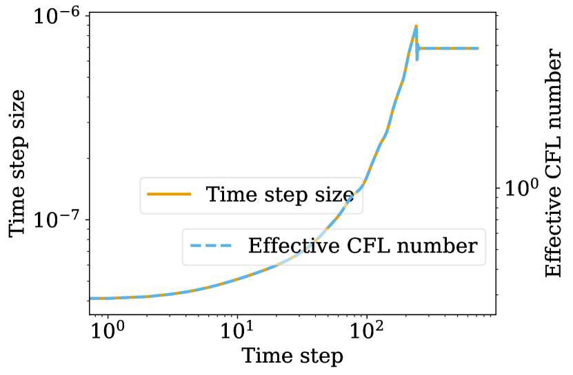
(c) RDPK3(2)5_F[3S*₊] (time step number).

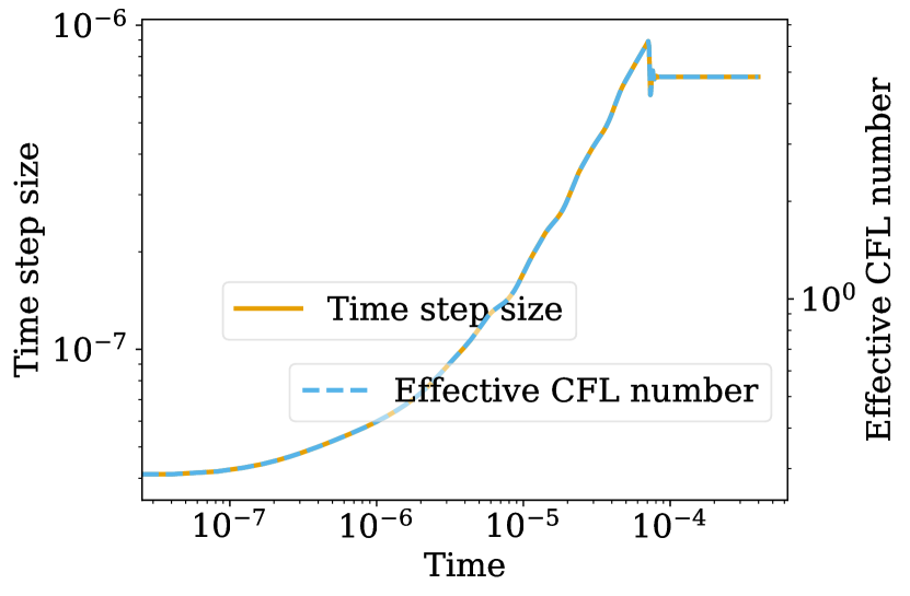
(d) RDPK3(2)5_F[3S*₊] (physical time).

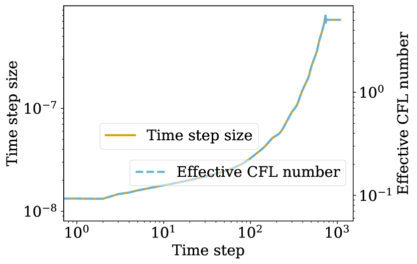
(e) SSP3(2)4[3S*₊] (time step number).

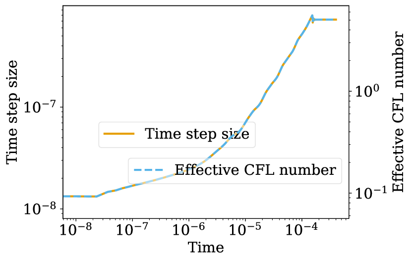
(f) SSP3(2)4[3S*₊] (physical time).

Figure 12: Effective CFL numbers and time step sizes depending on the time step index (left column) and physical time (right column) of some representative RK methods applied to entropy-dissipative semidiscretizations of the compressible Navier-Stokes equations for the delta wing setup.

Results of simulations using some representative RK methods are shown in Figure 12. For this cold start of the simulation with free stream values, all methods begin with a conservative estimate of the time step size. The error-based step size controllers increase the time step size in the first few time steps and reach an asymptotically constant step size after a few hundred time steps.

The effective CFL number shown in Figure 12 is basically proportional to the time step size itself. Running SSDC with CFL-based step size control requires a CFL factor that is (at least initially)

• $13\text{\,}\mathrm{\char 37\relax}$ smaller for BS3(2)3_F

• $21\text{\,}\mathrm{\char 37\relax}$ smaller for RDPK3(2)5_F[3S*₊]

• $32\text{\,}\mathrm{\char 37\relax}$ smaller for SSP3(2)4[3S*₊]

than the asymptotic CFL factor to avoid a blow-up of the simulation. The required number of right-hand side evaluations and rejected steps are listed in Table 2.

Table 2: Performance of representative RK methods with error-based step size controllers: Number of function evaluations (#FE), accepted steps (#A), and rejected steps (#R) for the delta wing setup up to time $t=0.015$.

Scheme	$\beta$	tol	#FE	#A	#R
BS3(2)3F	$(0.60,-0.20,0.00)$	$\texttt{tol}=10^{-8}$	$17\,641$	$5875$	$4$
RDPK3(2)5F[3S*+]	$(0.70,-0.23,0.00)$	$\texttt{tol}=10^{-8}$	$14\,963$	$2989$	$3$
SSP3(2)4[3S*+]	$(0.55,-0.27,0.05)$	$\texttt{tol}=10^{-8}$	$13\,392$	$3344$	$4$

5.4 NASA common research model

The NASA common research model (CRM) was conceived in 2007. Its aerodynamic design was completed in 2008, responding to needs broadly expressed within the US and international aeronautics communities for modern/industry-relevant geometries coupled with advanced experimental data for applied computational fluid dynamic validation studies [82]. Here, we consider the compressible Navier-Stokes equations for a flow over the NASA CRM at an angle of attack of $10\text{\,}\mathrm{\SIUnitSymbolDegree}$, a Mach number $\mathrm{Ma}=0.85$, and a Reynolds number of $\mathrm{Re}=5\times 10^{6}$.

The computational domain contains $12.8\times 10^{6}$ hexahedral elements with a maximum aspect ratio of approximately $105$. Entropy stable adiabatic no-slip wall boundary conditions [23] are applied to the aircraft, whereas freestream far-field boundary conditions are applied at the inlet and outlet planes. We set a solution polynomial degree $p=3$ in the whole domain. Given the degree of the solution and the number of cells, the number of DOFs is $\approx 7.68\times 10^{8}$. A zoom of the mesh near the surface of the right wing and the nacelle is shown in Figure 13.

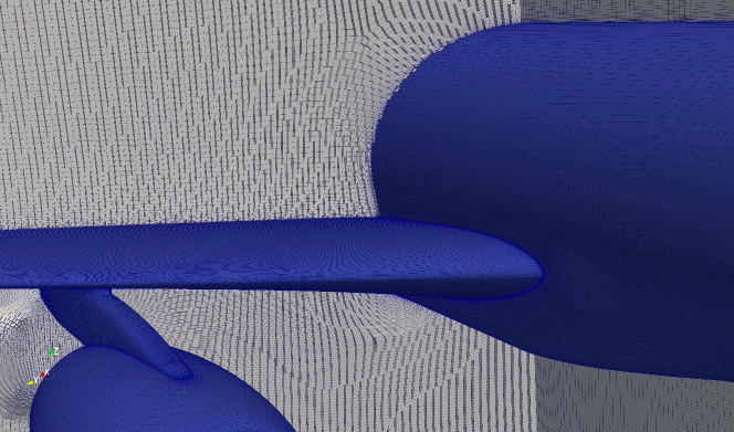
Figure 13: Zoom of the mesh for the NASA CRM generated at KAUST.

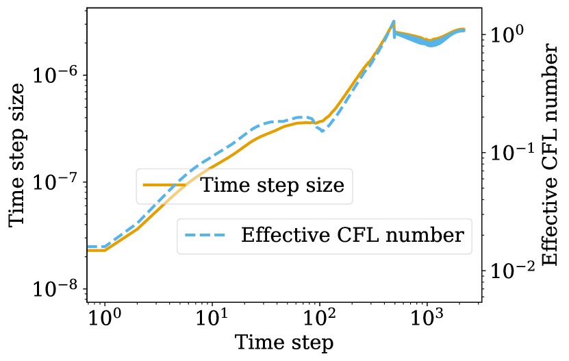
(a) BS3(2)3_F (time step number).

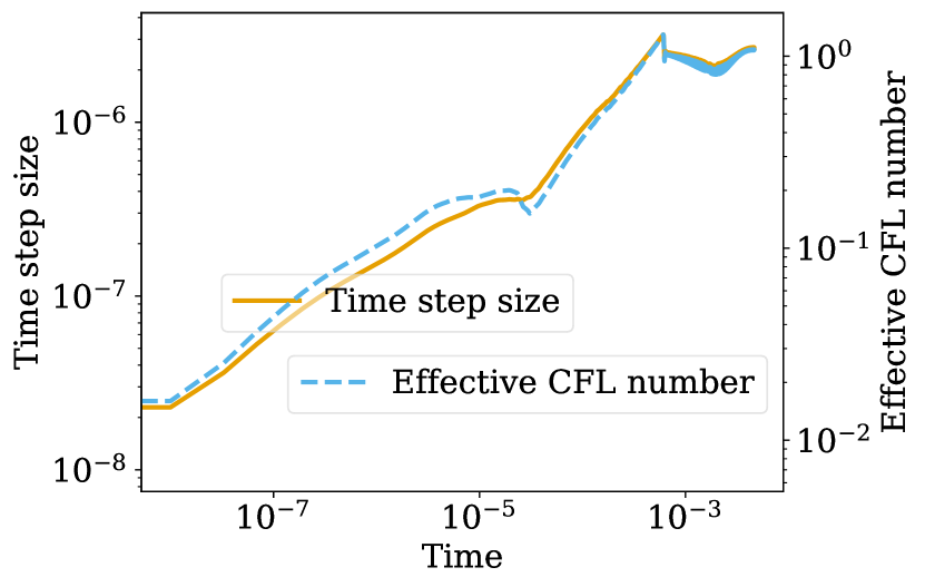
(b) BS3(2)3_F (physical time).

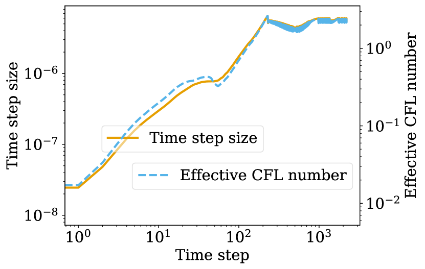
(c) RDPK3(2)5_F[3S*₊] (time step number).

(d) RDPK3(2)5_F[3S*₊] (physical time).

(e) SSP3(2)4[3S*₊] (time step number).

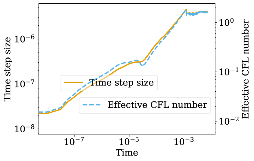
(f) SSP3(2)4[3S*₊] (physical time).

Figure 14: Effective CFL numbers and time step sizes depending on the time step index (left column) and physical time (right column) of some representative RK methods applied to entropy-dissipative semidiscretizations of the compressible Navier-Stokes equations for the NASA common research model.

Results of simulations using some representative RK methods are shown in Figure 14. Again, all methods use a conservative estimate of the initial time step size $\Delta t$, which then increases $\Delta t$ monotonically in the first few hundred time steps and reaches an asymptotically approximately constant step size afterwards. The effective CFL number shown in Figure 14 is, again, basically proportional to the time step size itself. Running SSDC with CFL-based step size control requires a CFL factor that is (at least initially)

• $16\text{\,}\mathrm{\char 37\relax}$ smaller for RDPK3(2)5_F[3S*₊]

• $9\text{\,}\mathrm{\char 37\relax}$ smaller for SSP3(2)4[3S*₊]

than the asymptotic CFL factor to avoid a blow-up of the simulation. For BS3(2)3_F, the asymptotic CFL factor from error-based step size control can be chosen for the complete simulation. The required number of right-hand side evaluations and rejected steps are listed in Table 3.

Table 3: Performance of representative RK methods with error-based step size controllers: Number of function evaluations (#FE), accepted steps (#A), and rejected steps (#R) for the NASA common research model up to time $t=0.004$.

Scheme	$\beta$	tol	#FE	#A	#R
BS3(2)3F	$(0.60,-0.20,0.00)$	$\texttt{tol}=10^{-8}$	$5874$	$1958$	$0$
RDPK3(2)5F[3S*+]	$(0.70,-0.23,0.00)$	$\texttt{tol}=10^{-8}$	$4610$	$922$	$0$
SSP3(2)4[3S*+]	$(0.55,-0.27,0.05)$	$\texttt{tol}=10^{-8}$	$5920$	$1480$	$0$

To conclude this test case, we highlight that the error-based controller yields a substantially higher level of robustness for this industry-relevant test case under a change of mesh structure. To verify that, we simulate the same flow problem using the mesh illustrated in Figure 15. This new mesh is one of the grids provided for the fifth high-order workshop held at Ceneaero, Belgium, and it corresponds to the mesh tagged as “CRM-WB-a2.75-Coarse-P2A”. When the CFL-based controller is used, the target CFL number is set to the effective asymptotic value obtained from the previous simulations with the mesh shown in Figure 13, i.e. approximately $3.6$ for all three RK methods (see Figure 14). The simulations run successfully to the final time for all the three time integration methods tested, i.e., BS3(2)3_F, RDPK3(2)5_F[3S*₊], and SSP3(2)4[3S*₊], when the error-based time step controller is used. On the contrary, all simulations fail when we choose the CFL-based time step controller. The reason is simple, the effective asymptotic value of the CFL number for this new mesh is approximately a factor of three smaller than the value set, i.e., $\approx 1.2$. This indicates that the CFL-based controller is not sufficiently robust under a change of mesh. In many cases, we could mitigate the instability by choosing a “very small value” for the target CFL number, but this would yield a very inefficient and computationally expensive time advancement of the simulation.

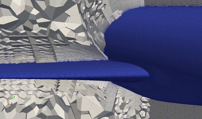
Figure 15: Zoom of the CRM-WB-a2.75-Coarse-P2A mesh for the NASA CRM provided by the fifth high-order workshop [13].

6 Change of variables: dissipative methods using an entropy projection

Whenever a semidiscretization is not strictly a collocation method, there are some transformations between the basic solution variables evolved in time and nodal values required to compute fluxes, e.g., methods using modal coefficients [62, 16], entropy variables as primary unknowns [46, 43], staggered grid methods [56, 68], and discontinuous Galerkin difference methods [98]. Here, we apply entropy-stable Gauss methods [17] available in Trixi.jl [80, 85] with efficient implementations [79]. While these schemes are more complex than collocation methods due to the entropy projection, they also possess favorable robustness properties for multidimensional simulations of under-resolved compressible flows with variable density and small-scale features [18].

We consider a Kelvin-Helmholtz instability of the 2D compressible Euler equations of an ideal gas with ratio of specific heats $\gamma=1.4$ as in [18]. The domain $[-1,1]^{2}$ is equipped with periodic boundary conditions and the simulation is initialized with

$$\begin{gathered}\varrho_{1}=1,\quad\varrho_{2}=\varrho_{1}\frac{1+A}{1-A},\quad\varrho^{0}=\varrho_{1}+B(x,y)(\varrho_{2}-\varrho_{1}),\\ p^{0}=1,\quad v_{1}^{0}=B(x,y)-\frac{1}{2},\quad v_{2}^{0}=\frac{1}{10}\sin(2\pi x),\end{gathered}$$ (6.1)

where $A$ is the Atwood number parameterizing the density contrast and

$$B(x,y)=\tanh(15y+7.5)-\tanh(15y-7.5)$$ (6.2)

is a smoothed step function. We apply Gauss methods with 32 elements per coordinate direction and polynomials of degree $p=3$. We choose the entropy conservative flux of [74, 75, 77] for the volume terms and a local Lax-Friedrichs flux at surfaces. We apply several representative RK methods to evolve the resulting entropy-dissipative semidiscretizations in time $t\in[0,5]$.

6.1 Mild initial conditions with low Atwood number

Table 4: Performance of representative RK methods with default error-based and manually tuned CFL-based step size controllers: Number of function evaluations (#FE), accepted steps (#A), and rejected steps (#R) for the Kelvin-Helmholtz instability with low Atwood number $A=3/7$ and entropy-dissipative Gauss collocation semidiscretizations using entropy projections.

Scheme	$\beta$	tol/$\nu$	#FE	#A	#R
BS3(2)3F	$(0.60,-0.20,0.00)$	$\texttt{tol}=10^{-4}$	$7542$	$2511$	$2$
		$\nu=0.57$	$7801$	$2600$
RDPK3(2)5F[3S*+]	$(0.70,-0.23,0.00)$	$\texttt{tol}=10^{-4}$	$6403$	$1278$	$2$
		$\nu=1.10$	$6856$	$1371$
RDPK4(3)9F[3S*+]	$(0.38,-0.18,0.01)$	$\texttt{tol}=10^{-5}$	$6537$	$722$	$4$
		$\nu=1.85$	$6922$	$769$
SSP3(2)4[3S*+]	$(0.55,-0.27,0.05)$	$\texttt{tol}=10^{-4}$	$5478$	$1367$	$2$
		$\nu=1.03$	$5672$	$1418$

Table 4 shows a summary of the performance statistics of some representative RK methods for a low Atwood number $A=3/7$. The CFL number $\nu$ were maximized manually up to three significant digits (so that the simulations did not crash). We used time integration methods with controllers recommended in [76] and a default tolerance $\texttt{tol}=10^{-4}$; we set $\texttt{tol}=10^{-5}$ for RDPK4(3)9_F[3S*₊] since the simulation crashed for the looser default tolerance.

The total number of function evaluations and time steps is always smaller with error-based step size control in this example, usually around $5\text{\,}\mathrm{\char 37\relax}$. In addition, the manual optimization of the CFL factor $\nu$ required several simulation runs. Note that the optimal CFL factors are different from the ones used for the Orzsag-Tang vortex while the same tolerances were used. For this setup, SSP3(2)4[3S*₊] is the most efficient method, followed by RDPK3(2)5_F[3S*₊].

6.2 Demanding initial conditions with high Atwood number

Increasing the density contrast makes this under-resolved test case more demanding [18]. Violations of positivity are more likely to occur and the sensitivity of the entropy variables for near-vacuum states can cause issues [15, 98]. In particular, the basic variables evolved in time for the Gauss methods violate positivity properties of the density/pressure around $t\approx 3$ even for strict CFL factors such as $\nu=0.05$ for SSP3(2)4[3S*₊] so that a standard CFL-based step size control is not possible. Similar problems occur for other RK methods.

Table 5: Performance of representative RK methods with default error-based and manually tuned CFL-based step size controllers: Number of function evaluations (#FE), accepted steps (#A), and rejected steps (#R) for the Kelvin-Helmholtz instability with high Atwood number $A=0.7$ and entropy-dissipative Gauss collocation semidiscretizations using entropy projections.

Scheme	$\beta$	tol/$\nu$	#FE	#A	#R
BS3(2)3F	$(0.60,-0.20,0.00)$	$\texttt{tol}=10^{-4}$	$9567$	$3185$	$3$
RDPK3(2)5F[3S*+]	$(0.70,-0.23,0.00)$	$\texttt{tol}=10^{-4}$	$8173$	$1621$	$13$
RDPK4(3)9F[3S*+]	$(0.38,-0.18,0.01)$	$\texttt{tol}=10^{-6}$	$10587$	$1175$	$1$
SSP3(2)4[3S*+]	$(0.55,-0.27,0.05)$	$\texttt{tol}=10^{-4}$	$6618$	$1640$	$14$

In contrast, error-based step size control works directly in most cases, as shown in Table 5. We only needed to use a stricter tolerance $\texttt{tol}=10^{-6}$ for RDPK4(3)9_F[3S*₊]. This RK method has more stages than the other methods, making it more difficult to adapt quickly to changing conditions. Again, SSP3(2)4[3S*₊] is the most efficient method, followed by RDPK3(2)5_F[3S*₊].

7 New systems: convenient exploratory research

A key feature of error-based time stepping methods is that they require no knowledge of the maximum eigenvalues to select a stable explicit time step. This feature is particularly convenient when one wants to apply existing numerical methods to new equation systems. To illustrate this, we consider the shallow water equations augmented with an Exner equation to account for interactions between the bottom topography and the fluid flow. The coupled system of equations in two spatial dimensions is

$$\frac{\partial}{\partial t}\begin{pmatrix}h\\[2.84544pt] hv_{1}\\[2.84544pt] hv_{2}\\[2.84544pt] b\end{pmatrix}+\frac{\partial}{\partial x}\begin{pmatrix}hv_{1}\\[2.84544pt] hv_{1}^{2}+\frac{g}{2}h^{2}\\[2.84544pt] hv_{1}v_{2}\\[2.84544pt] \xi q_{1}(\boldsymbol{v})\end{pmatrix}+\frac{\partial}{\partial y}\begin{pmatrix}hv_{2}\\[2.84544pt] hv_{1}v_{2}\\[2.84544pt] hv_{2}^{2}+\frac{g}{2}h^{2}\\[2.84544pt] \xi q_{2}(\boldsymbol{v})\end{pmatrix}=\begin{pmatrix}0\\[2.84544pt] -gh\frac{\partial b}{\partial x}\\[2.84544pt] -gh\frac{\partial b}{\partial y}\\[2.84544pt] 0\end{pmatrix},$$ (7.1)

where $h(x,y,t)$ is the water height, $\boldsymbol{v}(x,y,t)=(v_{1}(x,y,t),v_{2}(x,y,t))^{T}$ is the velocity field, $b(x,y,t)$ is the evolving bottom topography, and $g$ is the gravitational constant.

The last line in (7.1) is the Exner equation for the time evolution of the bottom topography $b$. It contains the constant $\xi=1/(1-\sigma)$ where $\sigma\in(0,1)$ is the porosity of the bottom material, and the solid transport discharge $\boldsymbol{q}=(q_{1},q_{2})^{T}$ as a function of the flow velocity $\boldsymbol{v}$. A closure model is required to describe how the bottom topography couples to the flow and defines the form of the $\boldsymbol{q}$ terms. This closure depends on the characteristics of the bottom material and flow, e.g., the grain size or Froude number. There exist many closure models for the solid transport discharge proposed and studied (analytically as well as numerically) in the literature, see e.g., [10, 30, 32, 64]. For the present study, we consider the simple and frequently used model due to Grass [32] that models the instantaneous sediment transport as a power law on the velocity field:

$$\boldsymbol{q}(\boldsymbol{v})=A_{g}\boldsymbol{v}\left(v_{1}^{2}+v_{2}^{2}\right)^{\frac{m-1}{2}}.$$ (7.2)

In (7.2), the constant $A_{g}\in[0,1]$ accounts for the porosity of the bottom sediment layer as well as the effects of the grain size and is usually determined from experimental data. When $A_{g}$ is zero there is no sediment transport and (7.1) reduces to the standard two-dimensional shallow water equations. The interaction between the bottom and the water flow is weak when $A_{g}$ is small and strong as $A_{g}$ approaches one. The factor $m\in[1,4]$ in the Grass model may also be determined from data; however, if one considers odd integer values of $m$, then (7.2) can be differentiated and the model remains valid for all values of the velocity field $\boldsymbol{v}$. For the remainder of this discussion we will take $m=3$ and the solid transport discharge will take the form

$$\boldsymbol{q}(\boldsymbol{v})=A_{g}\boldsymbol{v}\left(v_{1}^{2}+v_{2}^{2}\right).$$ (7.3)

For the particular closure model (7.3), we investigate the flux Jacobian of the governing system of equations (7.1). This is because the choice of a stable explicit time step under a CFL condition requires knowledge of the fastest wave speed of the underlying system. For this we compute the flux Jacobian in the $x$-direction, which incorporates non-conservative terms from the right hand side of (7.1), to be

$$\frac{\partial\boldsymbol{f}}{\partial\boldsymbol{u}}=\begin{pmatrix}0&1&0&0\\[4.26773pt] gh-v_{1}^{2}&2v_{1}&0&gh\\[4.26773pt] -v_{1}v_{2}&v_{2}&v_{1}&0\\[4.26773pt] -\frac{3\xi A_{g}v_{1}}{h}\left(v_{1}^{2}+v_{2}^{2}\right)&\frac{\xi A_{g}}{h}\left(3v_{1}^{2}+v_{2}\right)&\frac{2\xi A_{g}}{h}v_{1}v_{2}&0\end{pmatrix}.$$ (7.4)

Note that the analysis and results in the $y$-direction are analogous, so we will only consider (7.4) for this eigenvalue analysis for time step purposes. With the chosen Grass closure model it has been shown that all the eigenvalues of (7.4) are real and the governing system (7.1) is hyperbolic [19, 26]. The eigenvalues of the Jacobian in the $x$-direction are $v_{1}$ and the three roots of the characteristic polynomial

$$\lambda^{3}-2v_{1}\lambda^{2}+(v_{1}^{2}-gh-g\xi A_{g}(3v_{1}^{2}+v_{2}^{2}))\lambda+g\xi A_{g}v_{1}(3v_{1}^{2}+v_{2}^{2})=0.$$ (7.5)

It is possible, although unwieldy, to apply Cardano’s formula to determine the real, distinct roots of (7.5). However, an accurate estimate to the maximum wave speed from (7.5) is necessary for traditional CFL-based time stepping methods.

For many applications of interest the characteristic flow speed of the water is much faster than the speed of the bottom topography [19, 45, 92]. In particular, for subcritical flow the value of $v_{1}$ is relatively small, so it is possible to use a loose bound of the flow speeds with $v_{1}\pm\sqrt{gh}$ where $\sqrt{gh}$ is the surface wave speed. However, this loose bound applied to a CFL time step condition can result in excessive numerical diffusion that acts on the computed (slowly moving) bottom topography.

To approximate the solution of the shallow water equations with an Exner model (7.1) we use a discontinuous Galerkin spectral element method in space to create the semi-discretization and apply explicit time integration, see [95] for details. To couple the moving bottom topography $b(x,y,t)$ we use an unsteady approach where the water flow and riverbed are calculated simultaneously. That is, the water flow can be either steady or unsteady and the changes in the bed update are considered to be significant, i.e., the wave speed of the bed-updating equation is of a similar magnitude to the wave speeds of the water flow. For this approach, the system of flow and bottom evolution equations are discretised simultaneously. This high-order discontinuous Galerkin method applied to the shallow water equations is well-balanced for static and subcritical moving water flow [95, 96].

As an exemplary test case, we consider the evolution of a smooth sand hill bottom topography in a uniform flow governed by the shallow water equations. This test case is a two dimensional numerical simulation that was first proposed and analyzed by de Vriend [24]. It has become a common test case for benchmarking purposes in the moving bottom topography literature, e.g. [5, 19, 26, 45, 92], as it is easy to setup and demonstrates the ability of a numerical scheme to capture the morphology of a bottom topography governed with (7.1).

It involves the evolution of a conical sand dune in a channel with a non-erodible bottom on a square domain with dimensions $1000\text{\,}\mathrm{m}$ $\times$ $1000\text{\,}\mathrm{m}$. The initial conditions of the flow variables for this test case given in conservative variables are

$$\begin{pmatrix}h\\[2.84544pt] hv_{1}\\[2.84544pt] hv_{2}\\[2.84544pt] \end{pmatrix}=\begin{pmatrix}10-b(x,y,0)\\[2.84544pt] 10\\[2.84544pt] 0\\[2.84544pt] \end{pmatrix},$$ (7.6)

and the initial form of the sediment layer is given by

$$b(x,y,0)=\begin{cases}\sin^{2}\Bigl{(}\frac{(x-300)\pi}{200}\Bigr{)}\sin^{2}\Bigl{(}\frac{(y-400)\pi}{200}\Bigr{)}&\textrm{if }300\leq x\leq 500,\,400\leq y\leq 600,\\[2.84544pt] 0&\textrm{otherwise.}\end{cases}$$ (7.7)

We set the gravitational constant to be $g=$9.8\text{\,}\mathrm{m}\mathrm{/}\mathrm{s}^{2}$$. The porosity of the sediment material is $\sigma=0.4$ and the free parameter from the Grass model (7.3) is $A_{g}=0.001$. The parameter $A_{g}$ corresponds to the coupling strength and speed of interaction between the sediment and the water flow [5, 45]. Taking a small value for $A_{g}$ models weak coupling and a simulation must be run for a longer time period in order to observe significant variations in the sediment layer. Therefore, we take the final time of this simulation to be $t=100$ hours ($360{,}000$ seconds). The discharge value $hv_{1}=$10\text{\,}\mathrm{m}^{2}\mathrm{/}\mathrm{s}$$ from (7.6) gives the Froude number

$$\textrm{Fr}=\frac{\sqrt{v_{1}^{2}+v_{2}^{2}}}{\sqrt{gh}}\approx 0.1.$$ (7.8)

Thus, the flow is in the subcritical regime and we must set boundary conditions accordingly, see e.g. [65]. For this test case, the boundary conditions are taken to be walls on the top and bottom of the domain, the left is a subcritical inflow, and the right is a subcritical outflow. The complete setup can be found in the reproducibility repository [81].

For the spatial discretization we divide the domain $\Omega=[0,1000]^{2}$ into $900$ Cartesian elements. In each element we use polynomials of degree $p=5$ in each spatial direction for the discontinuous Galerkin approximation. This results in $32{,}400$ DOFs for each equation in (7.1). The classic shallow water equations for water height, momentum, and bottom topography terms are discretized with the well-balanced, high-order discontinuous Galerkin method described by Wintermeyer et al. [95]. The additional Exner equation for sediment transport is discretized with a standard discontinuous Galerkin spectral element approximation.

We first investigate the use of error-based time step control for this shallow water with sediment transport problem setup. We recorded the time step sizes and effective CFL numbers after every accepted time step for three representation RK methods. The tolerance is set to $\texttt{tol}=10^{-7}$ for all error-based time stepping methods considered. All three time integration techniques work directly for this test case. The behavior of the time step size and the effective CFL number are presented in Figure 16. Initially, the time step size of the three methods increases before the time step settles to a stable value as the physical problem becomes a quasi-steady flow where the sediment slowly evolves in the presence of the background flow.

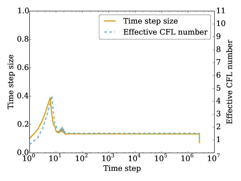
(a) BS3(2)3_F (time step number).

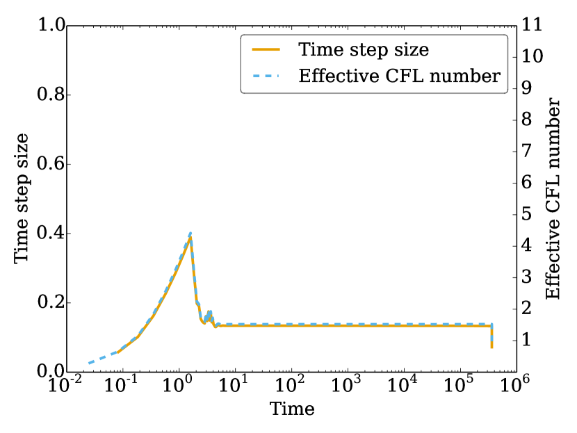
(b) BS3(2)3_F (physical time).

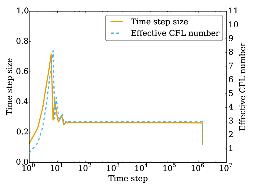
(c) RDPK3(2)5_F[3S*₊] (time step number).

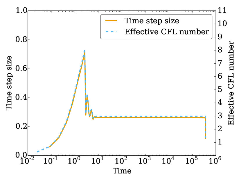
(d) RDPK3(2)5_F[3S*₊] (physical time).

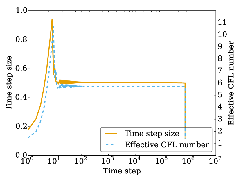
(e) RDPK4(3)9_F[3S*₊] (time step number).

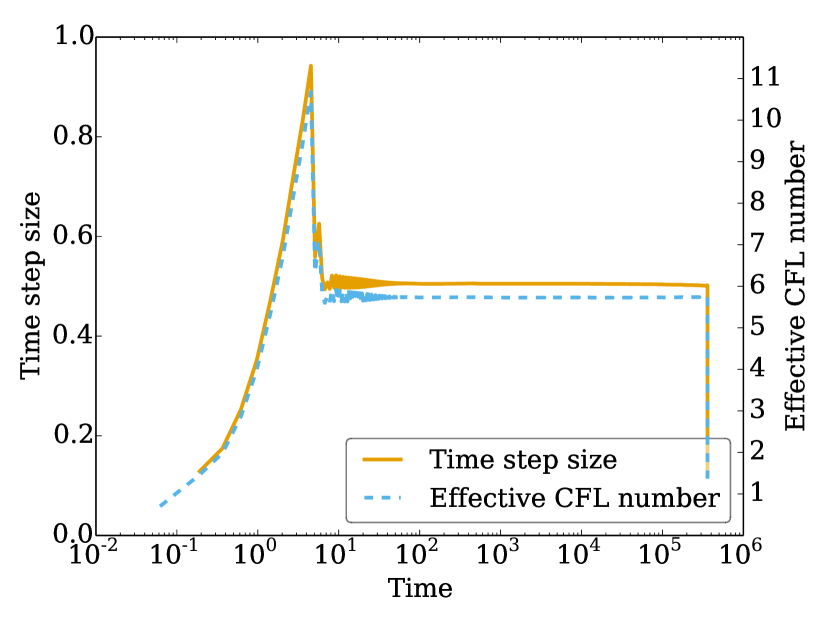
(f) RDPK4(3)9_F[3S*₊] (physical time).

Figure 16: Time step sizes and effective CFL numbers for three error-based RK methods. Left column: # time steps is $x$-axis. Right column: Time is $x$-axis.

We further investigate the effectiveness of the three time integrators with error-based step size control for this test case, as shown in Table 6. For this quasi-steady state configuration we found that a stricter tolerance $\texttt{tol}=10^{-7}$ for all the integration techniques tested performed the best in the sense of requiring a lower number of time steps. Here we find that RDPK4(3)9_F[3S*₊] is the most efficient method, followed by RDPK3(2)5_F[3S*₊].

Table 6: Performance of representative RK methods with default error-based and step size controllers: Number of function evaluations (#FE), accepted steps (#A), and rejected steps (#R) for a shallow water flow over an evolving sand dune.

Scheme	$\beta$	tol/$\nu$	#FE	#A	#R
BS3(2)3F	$(0.60,-0.20,0.00)$	$\texttt{tol}=10^{-7}$	$8{,}088{,}687$	$2{,}696{,}226$	$2$
RDPK3(2)5F[3S*+]	$(0.70,-0.23,0.00)$	$\texttt{tol}=10^{-7}$	$6{,}873{,}513$	$1{,}374{,}701$	$1$
RDPK4(3)9F[3S*+]	$(0.38,-0.18,0.01)$	$\texttt{tol}=10^{-7}$	$6{,}442{,}851$	$715{,}871$	$1$

We examine the expected solution behavior as well as simulation results for the sediment transport problem under consideration. As time evolves, the conical dune (7.7) gradually spreads into a star-shaped pattern. That is, the sediment will redistribute itself along a triangular shape with a particular spreading angle $\alpha$ and the bulk shape of the dune will move with a speed $c_{0}$ as it spreads [24, 45]. This process is illustrated in Figure 17.

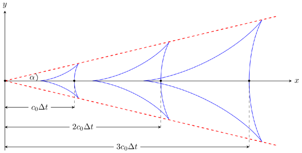
Figure 17: Characteristic evolution of a dune shaped sediment distribution.

When the Grass model is used and the interaction between the flow and sediment is weak, that is $A_{g}<0.01$, de Vriend [24] derived an analytical approximation for this spreading angle. In particular, when $m=3$ in the Grass model (7.3), this spreading angle of a conical dune is

$$\alpha=\tan^{-1}\left(\frac{3\sqrt{3}}{13}\right)\approx$21.787\text{\,}\mathrm{\SIUnitSymbolDegree}$.$$ (7.9)

Next, we present simulation results obtained using RDPK4(3)9_F[3S*₊], which was found to be the most efficient. The numerical results from the other two time integration techniques were similar and will not be presented. Figure 18 shows the bottom topography at the initial and final times. From this figure we see that the discretization captures the expected star-shaped pattern of the sediment evolution.

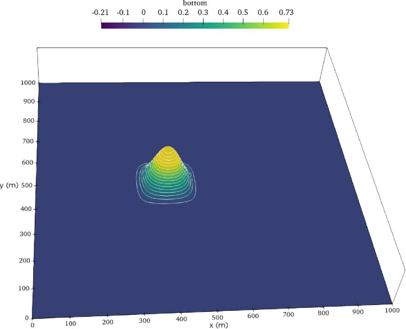
(a) $t=$0\text{\,}\mathrm{s}$$

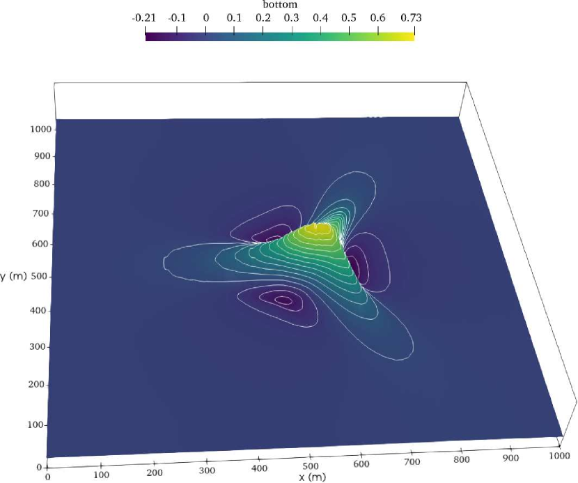
(b) $t=$360\,000\text{\,}\mathrm{s}$$

Figure 18: Projected lateral view of the approximate solution of the bottom topography $b(x,y,t)$ that demonstrates expected star-shaped structure of the conical sand dune at the final time.

We also estimate the spreading angle of a conical sand dune obtained for the numerical simulation [92]. This is done by examining the angle up to the iso-level $0.0125$ over time as shown in Figure 19. We are able to numerically estimate the spreading angle to be $\alpha_{\textrm{num}}=$20.4\text{\,}\mathrm{\SIUnitSymbolDegree}$$. The numerical spreading angle of the current method compares well to the theoretical angle (7.9) as well as to similar angle studies done in the literature [5, 26, 45, 92].

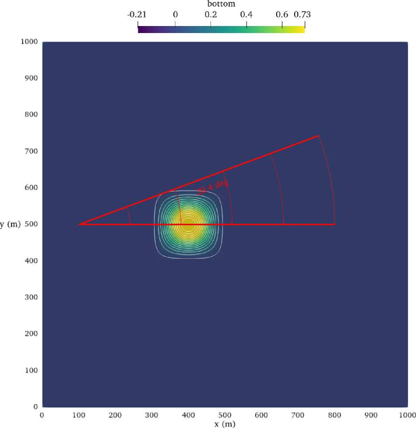
(a) $t=$0\text{\,}\mathrm{s}$$

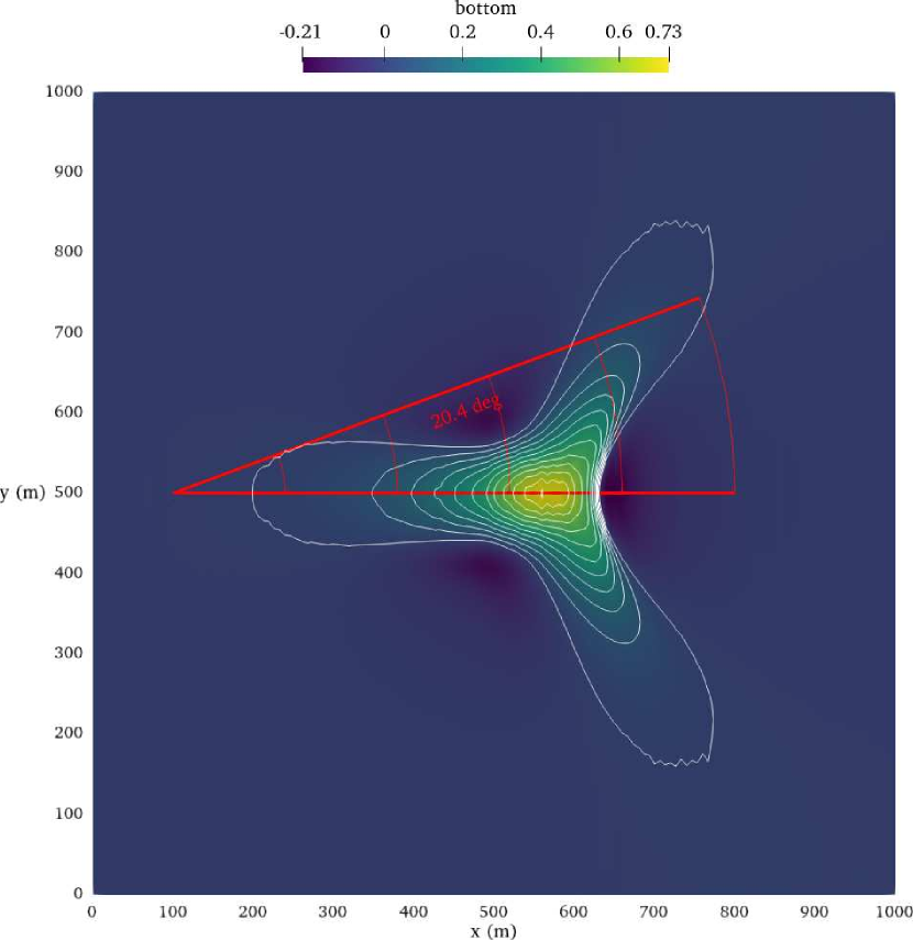
(b) $t=$360\,000\text{\,}\mathrm{s}$$

Figure 19: Estimation of the spreading angle $\alpha_{\textrm{num}}=$20.4\text{\,}\mathrm{\SIUnitSymbolDegree}$$ for the numerical approximation of a conical sand dune found by examining the iso-level $0.0125$ at the initial and final times. The theoretical prediction of the spreading angle for this problem setup is $21.787\text{\,}\mathrm{\SIUnitSymbolDegree}$.

We applied error-based time stepping methods to the shallow water equations augmented with an Exner equation to model sediment transport. This served to demonstrate that it is convenient and straightforward to extend existing code for a new system of equations and obtain a first set of numerical results. This was particularly useful for the considered shallow water Exner equations because eigenvalue estimates for a general problem setup are unwieldy to obtain [19, 26]. These preliminary results for the evolution and spreading of a conical sand dune compared well to the theoretical solution behavior as well as results from the literature. The development of high-order discontinuous Galerkin methods for sediment transport problems is the subject of ongoing research. Details about the physical problem setup and numerical parameters as well as all code necessary to reproduce the figures in this section are available in the reproducibility repository for this article [81].

8 Summary and conclusions

We have compared CFL- and error-based step size control of explicit Runge-Kutta methods applied to discontinuous Galerkin semidiscretizations of compressible CFD problems. Our numerical experiments demonstrate that error-based step size control is convenient and robust in a wide range of applications, including industrially relevant complex geometries with curved meshes in multiple dimensions, shock capturing schemes, initial transient periods (cold start of a simulation), semidiscretizations involving a change of variables, and for exploratory research involving new systems of equations.

There are cures for some problems of CFL-based step size control discussed in this article. For example, a cold start requiring an initially smaller CFL factor could run a few hundred time steps with a small CFL factor and use a larger CFL factor after a restart — or increase the CFL factor based on a user-supplied function in the first time steps. A change of linear stability behavior of shock capturing schemes could be handled by including the shock capturing indicator in CFL-based step size control. However, this requires sophisticated additional mechanisms as implemented in some in-house codes. On the other hand, error-based step size control worked right out of the box without further modifications for the problems considered here. It does not require special handling of many edge cases and comes with a reduced sensitivity with respect to user-supplied parameters.

While we have shown that error-based step size control is convenient and robust in many applications, including industrially relevant large-scale computations of compressible CFD problems, it does not come with hard mathematical guarantees. For example, some invariant domain preserving methods come with some robustness properties guaranteed under certain CFL constraints; error-based step size control alone can usually not be proven to satisfy these constraints in all cases. Nevertheless, based on our experience, it is usually robust for suitably chosen shock capturing mechanisms.

As a byproduct of this research, we also compared several time integration methods for hyperbolic conservation laws and compressible flow problems. For lower Mach number flows or problems with positivity issues and/or strong shock capturing requirements, SSP3(2)4[3S*₊] is usually the most efficient scheme. Otherwise, RDPK3(2)5_F[3S*₊] and RDPK4(3)9_F[3S*₊] are usually the most efficient methods, where RDPK3(2)5_F[3S*₊] tends to be more robust and RDPK4(3)9_F[3S*₊] tends to be more efficient for stricter tolerances. Nevertheless, BS3(2)3_F is still one of the best general-purpose ODE solvers for problems like the ones considered in this article.

Future research includes the investigation of error-based step size control with adaptive mesh refinement and stabilization techniques such as positivity preserving limiters [99]. These are usually implemented as callbacks outside of the inner time integration loop and are thus “not seen” by error estimators. Moreover, we would like to optimize new RK methods including error estimators and step size controllers for compressible CFD problems in other ranges than [2], e.g., focusing on lower-Mach flows and dissipative effects.

References

- [1] Shrirang Abhyankar et al. “PETSc/TS: A Modern Scalable ODE/DAE Solver Library”, 2018 arXiv:1806.01437 [math.NA]
- [2] Rasha Al Jahdali, Radouan Boukharfane, Lisandro Dalcin and Matteo Parsani “Optimized Explicit Runge-Kutta Schemes for Entropy Stable Discontinuous Collocated Methods Applied to the Euler and Navier-Stokes equations” In AIAA Scitech 2021 Forum, 2021, pp. 0633 DOI: 10.2514/6.2021-0633
- [3] Satish Balay et al. “PETSc Users Manual”, 2020
- [4] Tobias Becker et al. “From exaflop to exaflow” In Design, Automation & Test in Europe Conference & Exhibition (DATE), 2017 Leuven: European DesignAutomation Association, 2017, pp. 404–409 IEEE
- [5] Fayssal Benkhaldoun, Slah Sahmim and Mohammed Seaid “A two-dimensional finite volume morphodynamic model on unstructured triangular grids” In International Journal for Numerical Methods in Fluids 63.11 Wiley Online Library, 2010, pp. 1296–1327 DOI: 10.1002/fld.2129
- [6] Martin Berzins “Temporal error control for convection-dominated equations in two space dimensions” In SIAM Journal on Scientific Computing 16.3 SIAM, 1995, pp. 558–580 DOI: 10.1137/0916036
- [7] Jeff Bezanson, Alan Edelman, Stefan Karpinski and Viral B Shah “Julia: A Fresh Approach to Numerical Computing” In SIAM Review 59.1 SIAM, 2017, pp. 65–98 DOI: 10.1137/141000671
- [8] Przemyslaw Bogacki and Lawrence F Shampine “A 3(2) pair of Runge-Kutta formulas” In Applied Mathematics Letters 2.4 Elsevier, 1989, pp. 321–325 DOI: 10.1016/0893-9659(89)90079-7
- [9] Marvin Bohm et al. “An entropy stable nodal discontinuous Galerkin method for the resistive MHD equations. Part I: Theory and Numerical Verification” In Journal of Computational Physics Elsevier, 2018 DOI: 10.1016/j.jcp.2018.06.027
- [10] R Briganti, N Dodd, D Kelly and D Pokrajac “An efficient and flexible solver for the simulation of the morphodynamics of fast evolving flows on coarse sediment beaches” In International Journal for Numerical Methods in Fluids 69.4 Wiley Online Library, 2012, pp. 859–877 DOI: 10.1002/fld.2618
- [11] Carsten Burstedde, Lucas C Wilcox and Omar Ghattas “p4est: Scalable algorithms for parallel adaptive mesh refinement on forests of octrees” In SIAM Journal on Scientific Computing 33.3 SIAM, 2011, pp. 1103–1133 DOI: 10.1137/100791634
- [12] John Charles Butcher “Numerical Methods for Ordinary Differential Equations” Chichester: John Wiley & Sons Ltd, 2016 DOI: 10.1002/9781119121534
- [13] Cenaero “HiOCFD5, 5th International Workshop on High–Order CFD Methods”, 2018 URL: https://how5.cenaero.be
- [14] Noel Chalmers and Lilia Krivodonova “A robust CFL condition for the discontinuous Galerkin method on triangular meshes” In Journal of Computational Physics 403 Elsevier, 2020, pp. 109095 DOI: 10.1016/j.jcp.2019.109095
- [15] Jesse Chan “On discretely entropy conservative and entropy stable discontinuous Galerkin methods” In Journal of Computational Physics 362 Elsevier, 2018, pp. 346–374 DOI: 10.1016/j.jcp.2018.02.033
- [16] Jesse Chan “Skew-symmetric entropy stable modal discontinuous Galerkin formulations” In Journal of Scientific Computing 81.1 Springer, 2019, pp. 459–485 DOI: 10.1007/s10915-019-01026-w
- [17] Jesse Chan, David C Del Rey Fernández and Mark H Carpenter “Efficient entropy stable Gauss collocation methods” In SIAM Journal on Scientific Computing 41.5 SIAM, 2019, pp. A2938–A2966 DOI: 10.1137/18M1209234
- [18] Jesse Chan et al. “On the entropy projection and the robustness of high order entropy stable discontinuous Galerkin schemes for under-resolved flows” In Frontiers in Physics 10, 2022 DOI: 10.3389/fphy.2022.898028
- [19] Alina Chertock, Alexander Kurganov and Tong Wu “Operator splitting based central-upwind schemes for shallow water equations with moving bottom topography” In Communications in Mathematical Sciences 18.8, 2020 DOI: 10.4310/CMS.2020.v18.n8.a3
- [20] J. Chu and J. M. Luckring “Experimental surface pressure data obtained on delta wing across Reynolds number and Mach number ranges” In NASA-TM-4645, 1996
- [21] Sidafa Conde, Imre Fekete and John N Shadid “Embedded pairs for optimal explicit strong stability preserving Runge-Kutta methods” In Journal of Computational and Applied Mathematics 412, 2022, pp. 114325 DOI: 10.1016/j.cam.2022.114325
- [22] Richard Courant, Kurt O Friedrichs and Hans Lewy “Über die partiellen Differenzengleichungen der mathematischen Physik” In Mathematische Annalen 100.1 Springer, 1928, pp. 32–74 DOI: 10.1007/BF01448839
- [23] Lisandro Dalcin et al. “Conservative and entropy stable solid wall boundary conditions for the compressible Navier-Stokes equations: Adiabatic wall and heat entropy transfer” In Journal of Computational Physics 397 Elsevier, 2019, pp. 108775 DOI: 10.1016/j.jcp.2019.06.051
- [24] HJ De Vriend “2DH mathematical modelling of morphological evolutions in shallow water” In Coastal Engineering 11.1 Elsevier, 1987, pp. 1–27 DOI: 10.1016/0378-3839(87)90037-8
- [25] Dominik Derigs et al. “Ideal GLM-MHD: About the entropy consistent nine-wave magnetic field divergence diminishing ideal magnetohydrodynamics equations” In Journal of Computational Physics 364 Elsevier, 2018, pp. 420–467 DOI: 10.1016/j.jcp.2018.03.002
- [26] MJ Castro Diaz, Enrique D Fernández-Nieto, AM Ferreiro and C Parés “Two-dimensional sediment transport models in shallow water equations. A second order finite volume approach on unstructured meshes” In Computer Methods in Applied Mechanics and Engineering 198.33-36 Elsevier, 2009, pp. 2520–2538 DOI: 10.1016/j.cma.2009.03.001
- [27] John R Dormand and Peter J Prince “A family of embedded Runge-Kutta formulae” In Journal of Computational and Applied Mathematics 6.1 Elsevier, 1980, pp. 19–26 DOI: 10.1016/0771-050X(80)90013-3
- [28] Michael Dumbser, Olindo Zanotti, Raphaël Loubère and Steven Diot “A posteriori subcell limiting of the discontinuous Galerkin finite element method for hyperbolic conservation laws” In Journal of Computational Physics 278 Elsevier, 2014, pp. 47–75 DOI: 10.1016/j.jcp.2014.08.009
- [29] Travis C Fisher and Mark H Carpenter “High-order entropy stable finite difference schemes for nonlinear conservation laws: Finite domains” In Journal of Computational Physics 252 Elsevier, 2013, pp. 518–557 DOI: 10.1016/j.jcp.2013.06.014
- [30] Jose Garres-Diaz, Manuel J Castro Diaz, Julian Koellermeier and Tomás Morales Luna “Shallow water moment models for bedload transport problems”, 2020 arXiv:2008.08449 [physics.flu-dyn]
- [31] Gregor Josef Gassner, Andrew Ross Winters and David A Kopriva “Split Form Nodal Discontinuous Galerkin Schemes with Summation-By-Parts Property for the Compressible Euler Equations” In Journal of Computational Physics 327 Elsevier, 2016, pp. 39–66 DOI: 10.1016/j.jcp.2016.09.013
- [32] AJ Grass “Sediment transport by waves and currents”, 1981
- [33] Jean-Luc Guermond et al. “On the implementation of a robust and efficient finite element-based parallel solver for the compressible Navier-Stokes equations”, 2021 arXiv:2106.02159 [math.NA]
- [34] Jean-Luc Guermond, Murtazo Nazarov, Bojan Popov and Ignacio Tomas “Second-order invariant domain preserving approximation of the Euler equations using convex limiting” In SIAM Journal on Scientific Computing 40.5 SIAM, 2018, pp. A3211–A3239 DOI: 10.1137/17M1149961
- [35] Jean-Luc Guermond, Richard Pasquetti and Bojan Popov “Entropy viscosity method for nonlinear conservation laws” In Journal of Computational Physics 230.11 Elsevier, 2011, pp. 4248–4267 DOI: 10.1016/j.jcp.2010.11.043
- [36] Kjell Gustafsson “Control theoretic techniques for stepsize selection in explicit Runge-Kutta methods” In ACM Transactions on Mathematical Software (TOMS) 17.4 ACM, 1991, pp. 533–554 DOI: 10.1145/210232.210242
- [37] Kjell Gustafsson, Michael Lundh and Gustaf Söderlind “A PI stepsize control for the numerical solution of ordinary differential equations” In BIT Numerical Mathematics 28.2 Springer, 1988, pp. 270–287 DOI: 10.1007/BF01934091
- [38] Ernst Hairer, Syvert Paul Nørsett and Gerhard Wanner “Solving Ordinary Differential Equations I: Nonstiff Problems” 8, Springer Series in Computational Mathematics Berlin Heidelberg: Springer-Verlag, 2008 DOI: 10.1007/978-3-540-78862-1
- [39] Ernst Hairer and Gerhard Wanner “Solving Ordinary Differential Equations II: Stiff and Differential-Algebraic Problems” 14, Springer Series in Computational Mathematics Berlin Heidelberg: Springer-Verlag, 2010 DOI: 10.1007/978-3-642-05221-7
- [40] George Hall and Desmond J Higham “Analysis of stepsize selection schemes for Runge-Kutta codes” In IMA Journal of Numerical Analysis 8.3 Oxford University Press, 1988, pp. 305–310 DOI: 10.1093/imanum/8.3.305
- [41] Philip Heinisch, Katharina Ostaszewski and Hendrik Ranocha “Towards Green Computing: A Survey of Performance and Energy Efficiency of Different Platforms using OpenCL” In Proceedings of the International Workshop on OpenCL, IWOCL ’20, April 2020, Munich (Germany) New York, NY, USA: ACM, 2020 DOI: 10.1145/3388333.3403035
- [42] Sebastian Hennemann, Andrés M Rueda-Ramirez, Florian J Hindenlang and Gregor J Gassner “A provably entropy stable subcell shock capturing approach for high order split form DG for the compressible Euler equations” In Journal of Computational Physics 426 Elsevier, 2021, pp. 109935 DOI: 10.1016/j.jcp.2020.109935
- [43] Andreas Hiltebrand and Siddhartha Mishra “Entropy stable shock capturing space-time discontinuous Galerkin schemes for systems of conservation laws” In Numerische Mathematik 126.1 Springer, 2014, pp. 103–151 DOI: 10.1007/s00211-013-0558-0
- [44] Florian Hindenlang and Gregor J Gassner “A new entropy conservative two-point flux for ideal MHD equations derived from first principles.”, Presented at HONOM 2019: European workshop on high order numerical methods for evolutionary PDEs, theory and applications, 2019
- [45] Justin Hudson “Numerical techniques for morphodynamic modelling”, 2001
- [46] Thomas J R Hughes, L P Franca and M Mallet “A new finite element formulation for computational fluid dynamics: I. Symmetric forms of the compressible Euler and Navier-Stokes equations and the second law of thermodynamics” In Computer Methods in Applied Mechanics and Engineering 54.2 Elsevier, 1986, pp. 223–234 DOI: 10.1016/0045-7825(86)90127-1
- [47] D. Hummel and G. Redeker “A New Vortex Flow Experiment for Computer Code Validation” In RTO/AVT Symposium on Vortex Flow and High Angle of Attack Aerodynamics, Meeting Proc. RTO-MP-069, 2003, pp. 8–31
- [48] George Em Karniadakis and Spencer Sherwin “Spectral/hp element methods for computational fluid dynamics” Oxford: Oxford University Press, 2013 DOI: 10.1093/acprof:oso/9780198528692.001.0001
- [49] Christopher A Kennedy, Mark H Carpenter and R Michael Lewis “Low-storage, explicit Runge-Kutta schemes for the compressible Navier-Stokes equations” In Applied Numerical Mathematics 35.3 Elsevier, 2000, pp. 177–219 DOI: 10.1016/S0168-9274(99)00141-5
- [50] David I Ketcheson “Runge-Kutta methods with minimum storage implementations” In Journal of Computational Physics 229.5 Elsevier, 2010, pp. 1763–1773 DOI: 10.1016/j.jcp.2009.11.006
- [51] David I Ketcheson, Mikael Mortensen, Matteo Parsani and Nathanael Schilling “More efficient time integration for Fourier pseudo-spectral DNS of incompressible turbulence” In International Journal for Numerical Methods in Fluids 92.2 Wiley Online Library, 2020, pp. 79–93 DOI: 10.1002/fld.4773
- [52] Matthew G Knepley and Dmitry A Karpeev “Mesh algorithms for PDE with Sieve I: Mesh distribution” In Scientific Programming 17.3 IOS Press, 2009, pp. 215–230 DOI: 10.3233/SPR-2009-0249
- [53] Tzanio Kolev et al. “Efficient exascale discretizations: High-order finite element methods” In The International Journal of High Performance Computing Applications 35.6 SAGE Publications Sage UK: London, England, 2021, pp. 527–552 DOI: 10.1177/10943420211020803
- [54] David A Kopriva “Implementing Spectral Methods for Partial Differential Equations: Algorithms for Scientists and Engineers” New York: Springer Science & Business Media, 2009 DOI: 10.1007/978-90-481-2261-5
- [55] David A Kopriva and Edwin Jimenez “An Assessment of the Efficiency of Nodal Discontinuous Galerkin Spectral Element Methods” In Recent Developments in the Numerics of Nonlinear Hyperbolic Conservation Laws Berlin: Springer Berlin Heidelberg, 2013, pp. 223–235 DOI: 10.1007/978-3-642-33221-0_13
- [56] David A Kopriva and John H Kolias “A conservative staggered-grid Chebyshev multidomain method for compressible flows” In Journal of computational physics 125.1 Elsevier, 1996, pp. 244–261 DOI: 10.1006/jcph.1996.0091
- [57] Johannes Franciscus Bernardus Maria Kraaijevanger “Contractivity of Runge-Kutta methods” In BIT Numerical Mathematics 31.3 Springer, 1991, pp. 482–528 DOI: 10.1007/BF01933264
- [58] Ethan J Kubatko, Clint Dawson and Joannes J Westerink “Time step restrictions for Runge-Kutta discontinuous Galerkin methods on triangular grids” In Journal of Computational Physics 227.23 Elsevier, 2008, pp. 9697–9710 DOI: 10.1016/j.jcp.2008.07.026
- [59] Dmitri Kuzmin “Entropy stabilization and property-preserving limiters for discontinuous Galerkin discretizations of scalar hyperbolic problems” In Journal of Numerical Mathematics 29.4 De Gruyter, 2021, pp. 307–322 DOI: 10.1515/jnma-2020-0056
- [60] Yong Liu, Jianfang Lu and Chi-Wang Shu “An Essentially Oscillation-Free Discontinuous Galerkin Method for Hyperbolic Systems” In SIAM Journal on Scientific Computing 44.1 SIAM, 2022, pp. A230–A259 DOI: 10.1137/21M140835X
- [61] Matthias Maier and Martin Kronbichler “Efficient parallel 3D computation of the compressible Euler equations with an invariant-domain preserving second-order finite-element scheme” In ACM Transactions on Parallel Computing 8.3 ACM New York, NY, 2021, pp. 1–30 DOI: 10.1145/3470637
- [62] Andreas Meister, Sigrun Ortleb, Thomas Sonar and Martina Wirz “A comparison of the Discontinuous-Galerkin- and Spectral-Difference-Method on triangulations using PKD polynomials” In Journal of Computational Physics 231.23 Elsevier, 2012, pp. 7722–7729 DOI: 10.1016/j.jcp.2012.07.025
- [63] Andreas Meister, Sigrun Ortleb, Thomas Sonar and Martina Wirz “An extended discontinuous Galerkin and spectral difference method with modal filtering” In ZAMM - Journal of Applied Mathematics and Mechanics / Zeitschrift für Angewandte Mathematik und Mechanik 93.6-7 Wiley Online Library, 2013, pp. 459–464 DOI: 10.1002/zamm.201200051
- [64] Eugen Meyer-Peter and R Müller “Formulas for bed-load transport” In IAHSR 2nd meeting, Stockholm, appendix 2, 1948 IAHR
- [65] Jan Nordström and Andrew R Winters “A linear and nonlinear analysis of the shallow water equations and its impact on boundary conditions” In Journal of Computational Physics 463 Elsevier, 2022, pp. 111254 DOI: 10.1016/j.jcp.2022.111254
- [66] Steven A Orszag and Cha-Mei Tang “Small-scale structure of two-dimensional magnetohydrodynamic turbulence” In Journal of Fluid Mechanics 90.1 Cambridge University Press, 1979, pp. 129–143 DOI: 10.1017/S002211207900210X
- [67] Matteo Parsani et al. “High-order accurate entropy-stable discontinuous collocated Galerkin methods with the summation-by-parts property for compressible CFD frameworks: Scalable SSDC algorithms and flow solver” In Journal of Computational Physics 424 Elsevier, 2021, pp. 109844 DOI: 10.1016/j.jcp.2020.109844
- [68] Matteo Parsani, Mark H Carpenter, Travis C Fisher and Eric J Nielsen “Entropy Stable Staggered Grid Discontinuous Spectral Collocation Methods of any Order for the Compressible Navier-Stokes Equations” In SIAM Journal on Scientific Computing 38.5 SIAM, 2016, pp. A3129–A3162 DOI: 10.1137/15M1043510
- [69] Matteo Parsani, Mark H Carpenter and Eric J Nielsen “Entropy stable wall boundary conditions for the three-dimensional compressible Navier-Stokes equations” In Journal of Computational Physics 292 Elsevier, 2015, pp. 88–113 DOI: 10.1016/j.jcp.2015.03.026
- [70] Matteo Parsani, David I Ketcheson and Willem Deconinck “Optimized explicit Runge-Kutta schemes for the spectral difference method applied to wave propagation problems” In SIAM Journal on Scientific Computing 35.2 SIAM, 2013, pp. A957–A986 DOI: 10.1137/120885899
- [71] Will Pazner “Sparse invariant domain preserving discontinuous Galerkin methods with subcell convex limiting” In Computer Methods in Applied Mechanics and Engineering 382 Elsevier, 2021, pp. 113876 DOI: 10.1016/j.cma.2021.113876
- [72] Per-Olof Persson and Jaime Peraire “Sub-Cell Shock Capturing for Discontinuous Galerkin Methods” In 44th AIAA Aerospace Sciences Meeting and Exhibit, 2006 American Institute of AeronauticsAstronautics DOI: 10.2514/6.2006-112
- [73] Christopher Rackauckas and Qing Nie “DifferentialEquations.jl – A Performant and Feature-Rich Ecosystem for Solving Differential Equations in Julia” In Journal of Open Research Software 5.1 Ubiquity Press, 2017, pp. 15 DOI: 10.5334/jors.151
- [74] Hendrik Ranocha “Entropy Conserving and Kinetic Energy Preserving Numerical Methods for the Euler Equations Using Summation-by-Parts Operators” In Spectral and High Order Methods for Partial Differential Equations ICOSAHOM 2018 134, Lecture Notes in Computational Science and Engineering Cham: Springer, 2020, pp. 525–535 DOI: 10.1007/978-3-030-39647-3_42
- [75] Hendrik Ranocha “Generalised Summation-by-Parts Operators and Entropy Stability of Numerical Methods for Hyperbolic Balance Laws”, 2018
- [76] Hendrik Ranocha, Lisandro Dalcin, Matteo Parsani and David I. Ketcheson “Optimized Runge-Kutta Methods with Automatic Step Size Control for Compressible Computational Fluid Dynamics” In Communications on Applied Mathematics and Computation 4, 2021, pp. 1191–1228 DOI: 10.1007/s42967-021-00159-w
- [77] Hendrik Ranocha and Gregor J Gassner “Preventing pressure oscillations does not fix local linear stability issues of entropy-based split-form high-order schemes” In Communications on Applied Mathematics and Computation, 2021 DOI: 10.1007/s42967-021-00148-z
- [78] Hendrik Ranocha, Jan Glaubitz, Philipp Öffner and Thomas Sonar “Stability of artificial dissipation and modal filtering for flux reconstruction schemes using summation-by-parts operators” In Applied Numerical Mathematics 128 Elsevier, 2018, pp. 1–23 DOI: 10.1016/j.apnum.2018.01.019
- [79] Hendrik Ranocha et al. “Efficient implementation of modern entropy stable and kinetic energy preserving discontinuous Galerkin methods for conservation laws”, 2021 arXiv:2112.10517 [cs.MS]
- [80] Hendrik Ranocha et al. “Adaptive numerical simulations with Trixi.jl: A case study of Julia for scientific computing” In Proceedings of the JuliaCon Conferences 1.1 The Open Journal, 2022, pp. 77 DOI: 10.21105/jcon.00077
- [81] Hendrik Ranocha et al. “Reproducibility repository for "On error-based step size control for discontinuous Galerkin methods for compressible fluid dynamics"”, https://github.com/trixi-framework/paper-2022-stepsize_control, 2022 DOI: 10.5281/zenodo.7078946
- [82] M. B. Rivers “NASA Common Research Model: A History and Future Plans” In AIAA SciTech 2019 Forum 1, pp. 1–36 DOI: 10.2514/6.2019-3725
- [83] Diego Rojas et al. “On the robustness and performance of entropy stable discontinuous collocation methods” In Journal of Computational Physics 426 Elsevier, 2021, pp. 109891 DOI: 10.1016/j.jcp.2020.109891
- [84] Tony Saad and Mokbel Karam “Stable timestep formulas for high-order advection-diffusion and Navier-Stokes solvers” In Computers & Fluids 244 Elsevier, 2022, pp. 105564 DOI: 10.1016/j.compfluid.2022.105564
- [85] Michael Schlottke-Lakemper, Andrew R Winters, Hendrik Ranocha and Gregor J Gassner “A purely hyperbolic discontinuous Galerkin approach for self-gravitating gas dynamics” In Journal of Computational Physics 442 Elsevier, 2021, pp. 110467 DOI: 10.1016/j.jcp.2021.110467
- [86] Björn Sjögreen and HC Yee “High order entropy conservative central schemes for wide ranges of compressible gas dynamics and MHD flows” In Journal of Computational Physics 364 Elsevier, 2018, pp. 153–185 DOI: 10.1016/j.jcp.2018.02.003
- [87] Gustaf Söderlind “Automatic control and adaptive time-stepping” In Numerical Algorithms 31.1-4 Springer, 2002, pp. 281–310 DOI: 10.1023/A:1021160023092
- [88] Gustaf Söderlind “Digital filters in adaptive time-stepping” In ACM Transactions on Mathematical Software (TOMS) 29.1 ACM, 2003, pp. 1–26 DOI: 10.1145/641876.641877
- [89] Gustaf Söderlind “Time-step selection algorithms: Adaptivity, control, and signal processing” In Applied Numerical Mathematics 56.3-4 Elsevier, 2006, pp. 488–502 DOI: 10.1016/j.apnum.2005.04.026
- [90] Gustaf Söderlind and Lina Wang “Adaptive time-stepping and computational stability” In Journal of Computational and Applied Mathematics 185.2 Elsevier, 2006, pp. 225–243 DOI: 10.1016/j.cam.2005.03.008
- [91] Matthias Sonntag and Claus-Dieter Munz “Shock Capturing for Discontinuous Galerkin Methods using Finite Volume Subcells” In Finite Volumes for Complex Applications VII-Elliptic, Parabolic and Hyperbolic Problems 78, Springer Proceedings in Mathematics & Statistics Cham: Springer International Publishing, 2014, pp. 945–953 DOI: 10.1007/978-3-319-05591-6_96
- [92] Miguel Uh Zapata, Lucia Gamboa Salazar, Reymundo Itzá Balam and Kim Dan Nguyen “An unstructured finite-volume semi-coupled projection model for bed load sediment transport in shallow-water flows” In Journal of Hydraulic Research 59.4 Taylor & Francis, 2021, pp. 545–558 DOI: 10.1080/00221686.2020.1786740
- [93] Peter Vincent et al. “Towards green aviation with Python at petascale” In SC’16: Proceedings of the International Conference for High Performance Computing, Networking, Storage and Analysis, 2016, pp. 1–11 IEEE DOI: 10.1109/SC.2016.1
- [94] J Ware and M Berzins “Adaptive finite volume methods for time-dependent PDEs” In Modeling, Mesh Generation, and Adaptive Numerical Methods for Partial Differential Equations New York: Springer, 1995, pp. 417–430 DOI: 10.1007/978-1-4612-4248-2_20
- [95] Niklas Wintermeyer, Andrew Ross Winters, Gregor Josef Gassner and David A Kopriva “An entropy stable nodal discontinuous Galerkin method for the two dimensional shallow water equations on unstructured curvilinear meshes with discontinuous bathymetry” In Journal of Computational Physics 340 Elsevier, 2017, pp. 200–242 DOI: 10.1016/j.jcp.2017.03.036
- [96] Andrew Ross Winters and Gregor Josef Gassner “A comparison of two entropy stable discontinuous Galerkin spectral element approximations for the shallow water equations with non-constant topography” In Journal of Computational Physics 301 Elsevier, 2015, pp. 357–376 DOI: 10.1016/j.jcp.2015.08.034
- [97] Paul Woodward and Phillip Colella “The numerical simulation of two-dimensional fluid flow with strong shocks” In Journal of Computational Physics 54.1 Elsevier, 1984, pp. 115–173 DOI: 10.1016/0021-9991(84)90142-6
- [98] Ge Yan, Sharanjeet Kaur, Jeffery W Banks and Jason E Hicken “Entropy-stable discontinuous Galerkin difference methods for hyperbolic conservation laws”, 2021 arXiv:2103.03826 [math.NA]
- [99] Xiangxiong Zhang and Chi-Wang Shu “Maximum-principle-satisfying and positivity-preserving high-order schemes for conservation laws: survey and new developments” In Proceedings of the Royal Society of London A: Mathematical, Physical and Engineering Sciences 467.2134 The Royal Society, 2011, pp. 2752–2776 DOI: 10.1098/rspa.2011.0153