Out-of-distribution Representation Learning for Time Series Classification

Abstract

Time series classification is an important problem in real world. Due to its non-stationary property that the distribution changes over time, it remains challenging to build models for generalization to unseen distributions. In this paper, we propose to view time series classification from the distribution perspective. We argue that the temporal complexity of a time series dataset could attribute to unknown latent distributions that need characterize. To this end, we propose Diversify for out-of-distribution (OOD) representation learning on dynamic distributions of times series. Diversify takes an iterative process: it first obtains the ‘worst-case’ latent distribution scenario via adversarial training, then reduces the gap between these latent distributions. We then show that such algorithm is theoretically supported. Extensive experiments are conducted on seven datasets with different OOD settings across gesture recognition, speech commands recognition, wearable stress and affect detection, and sensor-based human activity recognition. Qualitative and quantitative results demonstrate that Diversify significantly outperforms other baselines and effectively characterizes the latent distributions. Code is available at: https://github.com/microsoft/robustlearn.

1 Introduction

Time series classification is one of the most challenging problems in the machine learning and statistics community (Fawaz et al., 2019; Du et al., 2021). One important nature of time series is the non-stationary property, indicating that its statistical features are changing over time. For years, there have been tremendous efforts for time series classification, such as hidden Markov models (Fulcher & Jones, 2014), RNN-based methods (Hüsken & Stagge, 2003), and Transformer-based approaches (Li et al., 2019; Drouin et al., 2022).

We propose to model time series from the distribution perspective to handle its dynamically changing distributions; more precisely, to learn out-of-distribution (OOD) representations for time series that generalizes to unseen distributions. The general OOD/domain generalization problem has been extensively studied (Wang et al., 2022; Lu et al., 2022; Krueger et al., 2021; Rame et al., 2022), where the key is to bridge the gap between known and unknown distributions. Despite existing efforts, OOD in time series remains less studied and more challenging. Compared to image classification, the dynamic distribution of time series data keeps changing over time, containing diverse distribution information that should be harnessed for better generalization.

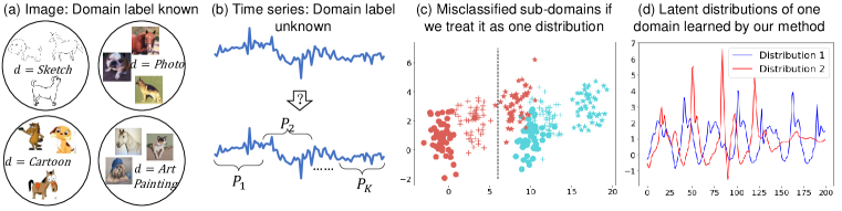
Figure 1: Illustration of Diversify: (a) Domain generalization for image data requires known domain labels. (b) Domain labels are unknown for time series. (c) If we treat the time series data as one single domain, the sub-domains are misclassified. Different colors and shapes correspond to different classes and domains. Axes represent data values. (d) Finally, our Diversify can effectively learn the latent distributions. X-axis represents data numbers while Y-axis represents values.

Figure 1 shows an illustrative example. OOD generalization in image classification often involves several domains whose domain labels are static and known (subfigure (a)), which can be employed to build OOD models. However, Figure 1 (b) shows that in EMG time series data (Lobov et al., 2018), the distribution is changing dynamically over time and its domain information is unavailable. If no attention is paid to exploring its latent distributions (i.e., sub-domains), predictions may fail in face of diverse sub-domain distributions (subfigure (c)). This will dramatically impede existing OOD algorithms due to their reliance on domain information.

In this work, we propose Diversify, an OOD representation learning algorithm for time series classification by characterizing the latent distributions inside the data. Concretely speaking, Diversify consists of a min-max adversarial game: on one hand, it learns to segment the time series data into several latent sub-domains by maximizing the segment-wise distribution gap to preserve diversities, i.e., the ‘worst-case’ distribution scenario; on the other hand, it learns domain-invariant representations by reducing the distribution divergence between the obtained latent domains. Such latent distributions naturally exist in time series, e.g., the activity data from multiple people follow different distributions. Additionally, our experiments show that even the data of one person still has such diversity: it can also be split into several latent distributions. Figure 1 (d) shows that Diversify can effectively characterize the latent distributions (more results are in Sec. 3.5).

To summarize, our contributions are four-fold:

• Novel perspective: We propose to view time series classification from the distribution perspective to learn OOD representation, which is more challenging than the traditional image classification due to the existence of unidentified latent distributions.

• Novel methodology: Diversify is a novel framework to identify the latent distributions and learn generalized representations. Technically, we propose pseudo domain-class labels and adversarial self-supervised pseudo labeling to obtain the pseudo domain labels.

• Theoretical insights: We provide the theoretical insights behind Diversify to analyze its design philosophy and conduct experiments to prove the insights.

• Superior performance and insightful results: Qualitative and quantitative results using various backbones demonstrate the superiority of Diversify in several challenging scenarios: difficult tasks, significantly diverse datasets, and limited data. More importantly, Diversify can successfully characterize the latent distributions within a time series dataset.

2 Methodology

A time-series training dataset $\mathcal{D}^{tr}$ can be often pre-processed using sliding window to $N$ inputs: $\mathcal{D}^{tr}=\{(\mathbf{x}_{i},y_{i})\}_{i=1}^{N}$, where $\mathbf{x}_{i}\in\mathcal{X}\subset\mathbb{R}^{p}$ is the $p$-dimensional instance and $y_{i}\in\mathcal{Y}=\{1,\ldots,C\}$ is its label. We use $\mathbb{P}^{tr}(\mathbf{x},y)$ on $\mathcal{X}\times\mathcal{Y}$ to denote the joint distribution of the training dataset. Our goal is to learn a generalized model from $\mathcal{D}^{tr}$ to predict well on an unseen target dataset, $\mathcal{D}^{te}$, which is inaccessible in training. In our problem, the training and test datasets have the same input and output spaces but different distributions, i.e., $\mathcal{X}^{tr}=\mathcal{X}^{te}$, $\mathcal{Y}^{tr}=\mathcal{Y}^{te}$, but $\mathbb{P}^{tr}(\mathbf{x},y)\neq\mathbb{P}^{te}(\mathbf{x},y)$. We aim to train a model $h$ from $\mathcal{D}^{tr}$ to achieve minimum error on $\mathcal{D}^{te}$.

2.1 Motivation

What are domain and distribution shift in time series? Time series may consist of several unknown latent distributions (domains), even if the dataset is fully labeled. For instance, data collected by sensors of three persons may belong to two different distributions due to their dissimilarities. This can be termed as spatial distribution shift. Surprisingly, we even find temporal distribution shifts in experiments (Figure 6(b)) that distributions of one person can also change at different time. Those shifts widely exist in time series, as suggested by  (Zhang et al., 2021; Ragab et al., 2022).

OOD generalization requires latent domain characterization. Due to the non-stationary property, naive approaches that treat time series as one distribution fail to capture domain-invariant (OOD) features since they ignore the diversities inside the dataset. In Figure 1 (c), we assume the training domain contains two sub-domains (circle and plus points). Directly treating it as one distribution via existing OOD approaches may generate the black margin. Red star points are misclassified to the green class when predicting on the OOD domain (star points) with the learned model. Thus, multiple diverse latent distributions in time series should be characterized to learn better OOD features.

A brief formulation of latent domain characterization. Following above discussions, a time series may consist of $K$ unknown latent domains rather than a fixed one, i.e., $\mathbb{P}^{tr}(\mathbf{x},y)=\sum_{i=1}^{K}\pi_{i}\mathbb{P}^{i}(\mathbf{x},y)$, where $\mathbb{P}^{i}(\mathbf{x},y)$ is the distribution of the $i$-th latent one with weight $\pi_{i}$, $\sum_{i=1}^{K}\pi_{i}=1$. There could be infinite ways to obtain $\mathbb{P}^{i}$s and our goal is to learn the ‘worst-case’ distribution scenario where the distribution divergence between each $\mathbb{P}^{i}$ and $\mathbb{P}^{j}$ is maximized. Why the ‘worst-case’ scenario? It will maximally preserve the diverse information of each latent distribution, thus benefiting generalization. For an illustration, these obtained latent distributions are shown in Sec. 3.5.

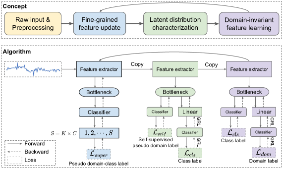
Figure 2: The framework of Diversify.

2.2 Diversify

In this paper, we propose Diversify to learn OOD representations for time series classification. The core of Diversify is to characterize the latent distributions and then minimize the distribution divergence between each two. Diversify utilizes an iterative process: it first obtains the ’worst-case’ distribution scenario from a given dataset, then bridges the distribution gaps between each pair of latent distributions. Figure 2 describes its main procedures, where steps $2\sim 4$ are iterative:

1. Pre-processing: this step adopts the sliding window to split the entire training dataset into fixed-size windows. We argue that the data from one window is the smallest domain unit.

2. Fine-grained feature update: this step updates the feature extractor using the proposed pseudo domain-class labels as the supervision.

3. Latent distribution characterization: it aims to identify the domain label for each instance to obtain the latent distribution information. It maximizes the different distribution gaps to enlarge diversity.

4. Domain-invariant representation learning: this step utilizes pseudo domain labels from the last step to learn domain-invariant representations and train a generalizable model.

Fine-grained Feature Update. Before characterizing the latent distributions, we perform fine-grained feature updates to obtain fine-grained representation. As shown in Figure 2 (blue), we propose a new concept: pseudo domain-class label to fully utilize the knowledge contained in domains and classes, which serves as the supervision for feature extractor. Features are more fine-grained w.r.t. domains and labels, instead of only attached to domains or labels.

At the first iteration, there is no domain label $d^{\prime}$ and we simply initialize $d^{\prime}=0$ for all samples. We treat per category per domain as a new class with label $s\in\{1,2,\cdots,S\}$. We have $S=K\times C$ where $K$ is the pre-defined number of latent distributions that can be tuned in experiments. We perform pseudo domain-class label assignment to get discrete values for supervision: $s=d^{\prime}\times C+y.$

Let $h_{f}^{(2)},h_{b}^{(2)},h_{c}^{(2)}$ be feature extractor, bottleneck, and classifier, respectively (we use superscripts to denote step number). Then, the supervised loss is computed using the cross-entropy loss $\ell$:

$$\mathcal{L}_{super}=\mathbb{E}_{(\mathbf{x},y)\sim\mathbb{P}^{tr}}\ell\left(h_{c}^{(2)}(h_{b}^{(2)}(h_{f}^{(2)}(\mathbf{x}))),s\right).$$ (1)

Latent Distribution Characterization. This step characterizes the latent distributions contained in one dataset. As shown in Figure 2 (green), we propose an adapted version of adversarial training to disentangle the domain labels from the class labels. However, there are no actual domain labels provided, which hinders such disentanglement. Inspired by (Caron et al., 2018), we employ a self-supervised pseudo-labeling strategy to obtain domain labels.

First, we attain the centroid for each domain with class-invariant features:

$$\tilde{\mu}_{k}=\frac{\sum_{\mathbf{x}_{i}\in\mathcal{X}^{tr}}\delta_{k}(h_{c}^{(3)}(h_{b}^{(3)}(h_{f}^{(3)}(\mathbf{x}_{i}))))h_{b}^{(3)}(h_{f}^{(3)}(\mathbf{x}_{i}))}{\sum_{\mathbf{x}_{i}\in\mathcal{X}^{tr}}\delta_{k}(h_{c}^{(3)}(h_{b}^{(3)}(h_{f}^{(3)}(\mathbf{x}_{i}))))},$$ (2)

where $h_{f}^{(3)},h_{b}^{(3)},h_{c}^{(3)}$ are feature extractor, bottleneck, and classifier, respectively. $\tilde{\mu}_{k}$ is the initial centroid of the $k^{th}$ latent domain while $\delta_{k}$ is the $k^{th}$ element of the logit soft-max output. Then, we obtain the pseudo domain labels via the nearest centroid classifier using a distance function $D$:

$$\tilde{d}^{\prime}_{i}=\arg\min_{k}D(h^{(3)}_{b}(h^{(3)}_{f}(\mathbf{x}_{i})),\tilde{\mu}_{k}).$$ (3)

Then, we compute the centroids and obtain the updated pseudo domain labels:

$$\mu_{k}=\frac{\sum_{\mathbf{x}_{i}\in\mathcal{X}^{tr}}\mathbb{I}(\tilde{d}^{\prime}_{i}=k)h^{(3)}_{b}(h^{(3)}_{f}(\mathbf{x}))}{\sum_{\mathbf{x}_{i}\in\mathcal{X}^{tr}}\mathbb{I}(\tilde{d}^{\prime}_{i}=k)},d^{\prime}_{i}=\arg\min_{k}D(h^{(3)}_{b}(h^{(3)}_{f}(\mathbf{x}_{i})),\mu_{k}),$$ (4)

where $\mathbb{I}(a)=1$ when $a$ is true, otherwise $0$. After obtaining $d^{\prime}$, we can compute the loss of step 2:

$$\mathcal{L}_{self}+\mathcal{L}_{cls}= \mathbb{E}_{(\mathbf{x},y)\sim\mathbb{P}^{tr}}\ell(h^{(3)}_{c}(h^{(3)}_{b}(h^{(3)}_{f}(\mathbf{x}))),d^{\prime})+\ell(h^{(3)}_{adv}(R_{\lambda_{1}}(h^{(3)}_{b}(h^{(3)}_{f}(\mathbf{x})))),y),$$ (5)

where $h^{(3)}_{adv}$ is the discriminator for step 3 that contains several linear layers and one classification layer. $R_{\lambda_{1}}$ is the gradient reverse layer with hyperparameter $\lambda_{1}$ (Ganin et al., 2016). After this step, we can obtain pseudo domain label $d^{\prime}$ for $\mathbf{x}$.

Domain-invariant Representation Learning. After obtaining the latent distributions, we learn domain-invariant representations for generalization. In fact, this step (purple in Figure 2) is simple: we borrow the idea from DANN (Ganin et al., 2016) and directly use adversarial training to update the classification loss $\mathcal{L}_{cls}$ and domain classifier loss $\mathcal{L}_{dom}$ using gradient reversal layer (GRL) (a common technique that facilitates adversarial training via reversing gradients) (Ganin et al., 2016):

$$\mathcal{L}_{cls}+\mathcal{L}_{dom}= \mathbb{E}_{(\mathbf{x},y)\sim\mathbb{P}^{tr}}\ell(h_{c}^{(4)}(h_{b}^{(4)}(h_{f}^{(4)}(\mathbf{x}))),y)+\ell(h_{adv}^{(4)}(R_{\lambda_{2}}(h_{b}^{(4)}(h_{f}^{(4)}(\mathbf{x})))),d^{\prime}),$$ (6)

where $\ell$ is the cross-entropy loss and $R_{\lambda_{2}}$ is the gradient reverse layer with hyperparameter $\lambda_{2}$ (Ganin et al., 2016). We will omit the details of GRL and adversarial training here since they are common techniques in deep learning. More details are presented in Appendix B.2.

Training, Inference, and Complexity. We repeat these steps until convergence or max epochs. Different from existing methods, the last two steps only optimize the last few independent layers but not the feature extractor. We perform inference with the modules from the last step. Most of the trainable parameters are shared between modules, indicating that Diversify has the same model size as existing methods and can reach quick convergence in experiments (Figure 14).

2.3 Theoretical Insights

We present some theoretical insights to show that our approach is well motivated in theory. Proofs can be found in Appendix A.

Proposition 2.1.

Let $\mathcal{X}$ be a space and $\mathcal{H}$ be a class of hypotheses corresponding to this space. Let $\mathbb{Q}$ and the collection $\{\mathbb{P}_{i}\}_{i=1}^{K}$ be distributions over $\mathcal{X}$ and let $\{\varphi_{i}\}_{i=1}^{K}$ be a collection of non-negative coefficient with $\sum_{i}\varphi_{i}=1$. Let $\mathcal{O}$ be a set of distributions s.t. $\forall\mathbb{S}\in\mathcal{O}$, the following holds

$$d_{\mathcal{H}\Delta\mathcal{H}}(\sum_{i}\varphi_{i}\mathbb{P}_{i},\mathbb{S})\leq\max_{i,j}d_{\mathcal{H}\Delta\mathcal{H}}(\mathbb{P}_{i},\mathbb{P}_{j}).$$ (7)

Then, for any $h\in\mathcal{H}$,

$$\varepsilon_{\mathbb{Q}}(h)\leq\lambda^{\prime}+\sum_{i}\varphi_{i}\varepsilon_{\mathbb{P}_{i}}(h)+\frac{1}{2}\min_{\mathbb{S}\in\mathcal{O}}d_{\mathcal{H}\Delta\mathcal{H}}(\mathbb{S},\mathbb{Q})+\frac{1}{2}\max_{i,j}d_{\mathcal{H}\Delta\mathcal{H}}(\mathbb{P}_{i},\mathbb{P}_{j}),$$ (8)

where $\lambda^{\prime}$ is the error of an ideal joint hypothesis. $\varepsilon_{\mathbb{P}}(h)$ is the error for a hypothesis $h$ on a distribution $\mathbb{P}$. $d_{\mathcal{H}\Delta\mathcal{H}}(\mathbb{P},\mathbb{Q})$ is $\mathcal{H}$-divergence which measures differences in distribution (Ben-David et al., 2010).

The first item in Eq. (8), $\lambda^{\prime}$, is often neglected since it is small in reality. The second item, $\sum_{i}\varphi_{i}\varepsilon_{\mathbb{P}_{i}}(h)$, exists in almost all methods and can be minimized via supervision from class labels with cross-entropy loss in Eq. (6). Our main purpose is to minimize the last two items in Eq. (8). Here $\mathbb{Q}$ corresponds to the unseen out-of-distribution target domain.

The last term $\frac{1}{2}\max_{i,j}d_{\mathcal{H}\Delta\mathcal{H}}(\mathbb{P}_{i},\mathbb{P}_{j})$ is common in OOD theory which measures the maximum differences among source domains. This corresponds to step 4 in our approach.

Finally, the third item, $\frac{1}{2}\min_{\mathbb{S}\in\mathcal{O}}d_{\mathcal{H}\Delta\mathcal{H}}(\mathbb{S},\mathbb{Q})$, explains why we exploit sub-domains in step 3. Since our goal is to learn a model which can perform well on an unseen target domain, we cannot obtain $\mathbb{Q}$. To minimize $\frac{1}{2}\min_{\mathbb{S}\in\mathcal{O}}d_{\mathcal{H}\Delta\mathcal{H}}(\mathbb{S},\mathbb{Q})$, we can only enlarge the range of $\mathcal{O}$. We have to $\max_{i,j}d_{\mathcal{H}\Delta\mathcal{H}}(\mathbb{P}_{i},\mathbb{P}_{j})$ according to Eq. (7), corresponding to step 3 in our method which tries to segment the time series data into several latent sub-domains by maximizing the segment-wise distribution gap to preserve diversities, i.e., the ‘worst-case’ distribution scenario.

3 Experiments

We perform evaluations on four diverse time series classification tasks: gesture recognition, speech commands recognition, wearable stress&affect detection, and sensor-based activity recognition.

Time series OOD algorithms are currently less studied and there are only two recent strong approaches for comparison: GILE (Qian et al., 2021) and AdaRNN (Du et al., 2021). We further compare with 7 general OOD methods from DomainBed (Gulrajani & Lopez-Paz, 2021): ERM, DANN (Ganin et al., 2016), CORAL (Sun & Saenko, 2016), Mixup (Zhang et al., 2018), GroupDRO (Sagawa et al., 2020), RSC (Huang et al., 2020), and ANDMask (Parascandolo et al., 2021). More details of these methods are in Sec. B.2 and B.3. For fairness, all methods (except GILE and AdaRNN) use a feature net with two blocks and each block has one convolution layer, one pooling layer, and one batch normalization layer, following (Wang et al., 2019). We also use Transformers (Vaswani et al., 2017) for backbone. Detailed data pre-processing, architecture, and hyperparameters are in Appendix C.5 and D. Ablations with various backbones are in Figure 8 and Appendix F.4.

Most OOD methods require the domain labels known in training while ours does not, which is more challenging and practical. We conduct the training-domain-validation strategy and the training data are split by $8:2$ for training and validation. We tune all methods to report the average best performance of three trials for fairness. Note that the “target” in experiments is unseen and only used for testing. $K$ in Diversify is treated as a hyperparameter and we tune it to record the best OOD performance. Per-segment accuracy is the evaluation metric. Time complexity and convergence are in Sec. F.5, showing its quick convergence.

3.1 Gesture Recognition

Table 1: Results on EMG dataset. “Target” $0\sim 4$ denotes unseen test distribution that is only for testing.

Target	0	1	2	3	AVG
ERM	62.6	69.9	67.9	69.3	67.4
DANN	62.9	70.0	66.5	68.2	66.9
CORAL	66.4	74.6	71.4	74.2	71.7
Mixup	60.7	69.9	70.5	68.2	67.3
GroupDRO	67.6	77.4	73.7	72.5	72.8
RSC	70.1	74.6	72.4	71.9	72.2
ANDMask	66.5	69.1	71.4	68.9	69.0
AdaRNN	68.8	81.1	75.3	78.1	75.8
Diversify	71.7	82.4	76.9	77.3	77.1

First, we evaluate Diversify on EMG for gestures Data Set (Lobov et al., 2018). It contains data of 36 subjects with 7 classes and we select 6 common classes for our experiments. We randomly divide 36 subjects into four domains (i.e., $0,1,2,3$). More details on EMG and domain splits can be found in Sec. C.2 and C.6 respectively. EMG data is affected by many factors since it comes from bioelectric signals.EMG data are scene and device-dependent, which means the same person may generate different data when performing the same activity with the same device at a different time (i.e., distribution shift across time (Wilson et al., 2020; Purushotham et al., 2016)) or with the different devices at the same time. Thus, the EMG benchmark is challenging. Table 1 shows that with the same backbone, our method achieves the best average performance and is $\mathbf{4.3}\%$ better than the second-best method. Diversify even outperforms AdaRNN which has a stronger backbone.

3.2 Speech Commands

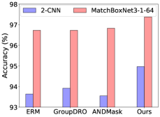
Figure 3: Results on Speech commands with two different backbones.

Then, we adopt a regular speech recognition task, the Speech Commands dataset (Warden, 2018). It consists of one-second audio recordings of both background noise and spoken words such as ‘left’ and ‘right’. It is collected from more than 2,000 persons, thus is more complicated. Following (Kidger et al., 2020), we use 34,975 time series corresponding to ten spoken words to produce a balanced classification problem. Since this dataset is collected from multiple persons, the training and test distributions are different, which is also an OOD problem with one training domain. There are many subjects and each subject only records a few audios. Thus, we do not split each sample. Figure 3 shows the results on two different backbones. Compared with GroupDRO, Diversify has over $\mathbf{1}\%$ improvement with a basic CNN backbone and over $\mathbf{0.6}\%$ improvement with a strong backbone MatchBoxNet3-1-64 (Majumdar & Ginsburg, 2020). It demonstrates the superiority of our method on a regular time-series benchmark containing massive distributions.

3.3 Wearable Stress and Affect Detection

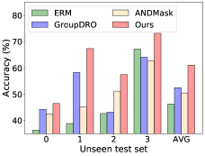
Figure 4: Results on WESAD. Here, $0\sim 4$ in x-axis denotes the unseen test dataset.

We further evaluate Diversify on a larger dataset, Wearable Stress and Affect Detection (WESAD) (Schmidt et al., 2018). WESAD is a public dataset that contains physiological and motion data of 15 subjects with $63,000,000$ instances. We utilize sensor modalities of chest-worn devices including electrocardiogram, electrodermal activity, electromyogram, respiration, body temperature, and three axis acceleration. We split 15 subjects into four domains (details are in Sec. C.6). Results Figure 4 showed that our method achieves the best performance compared to other state-of-the-art methods with an improvement of over $\textbf{8}\%$ on this larger dataset.

3.4 Sensor-based Human Activity Recognition

Finally, we construct four diverse OOD settings by leveraging four sensor-based human activity recognition datasets: DSADS (Barshan & Yüksek, 2014), USC-HAD (Zhang & Sawchuk, 2012), UCI-HAR (Anguita et al., 2012), and PAMAP (Reiss & Stricker, 2012). These datasets are collected from different people and positions using accelerometer and gyroscope, with $11,741,000$ instances in total. (1) Cross-person generalization aims to learn generalized models for different persons. (2) Cross-position generalization aims to learn generalized models for different sensor positions. (3) Cross-dataset generalization aims to learn generalized models for different datasets. (4) One-Person-To-Another aims to learn generalized models for different persons from data of a single person. For simplicity, we use $0,1,\cdots$ to denote different domains. More details on datasets information, setting construction, and domain splits can be found in Sec. C.3, C.4, and C.6.

Table 2: Accuracy on cross-person generalization. “Target” $0\sim 4$ denotes the unseen test set.

	DSADS					USC-HAD					PAMAP					ALL
Target	0	1	2	3	AVG	0	1	2	3	AVG	0	1	2	3	AVG	AVG
ERM	83.1	79.3	87.8	71.0	80.3	81.0	57.7	74.0	65.9	69.7	90.0	78.1	55.8	84.4	77.1	75.7
DANN	89.1	84.2	85.9	83.4	85.6	81.2	57.9	76.7	70.7	71.6	82.2	78.1	55.4	87.3	75.7	77.7
CORAL	91.0	85.8	86.6	78.2	85.4	78.8	58.9	75.0	53.7	66.6	86.2	77.8	49.0	87.8	75.2	75.7
Mixup	89.6	82.2	89.2	86.9	87.0	80.0	64.1	74.3	61.3	69.9	89.4	80.3	58.4	87.7	79.0	78.6
GroupDRO	91.7	85.9	87.6	78.3	85.9	80.1	55.5	74.7	60.0	67.6	85.2	77.7	56.2	85.0	76.0	76.5
RSC	84.9	82.3	86.7	77.7	82.9	81.9	57.9	73.4	65.1	69.6	87.1	76.9	60.3	87.8	78.0	76.9
ANDMask	85.0	75.8	87.0	77.6	81.4	79.9	55.3	74.5	65.0	68.7	86.7	76.4	43.6	85.6	73.1	74.4
GILE	81.0	75.0	77.0	66.0	74.7	78,0	62.0	77.0	63.0	70.0	83.0	68.0	42.0	76.0	67.5	70.7
AdaRNN	80.9	75.5	90.2	75.5	80.5	78.6	55.3	66.9	73.7	68.6	81.6	71.8	45.4	82.7	70.4	73.2
Diversify	90.4	86.5	90.0	86.1	88.2	82.6	63.5	78.7	71.3	74.0	91.0	84.3	60.5	87.7	80.8	81.0

Table 3: Classification accuracy on cross-position, cross-dataset, and one-to-another generalization.

	Cross-position generalization						Cross-dataset generalization					One-Person-To-Another
Target	0	1	2	3	4	AVG	0	1	2	3	AVG	DSADS	USC-HAD	PAMAP	AVG
ERM	41.5	26.7	35.8	21.4	27.3	30.6	26.4	29.6	44.4	32.9	33.3	51.3	46.2	53.1	50.2
DANN	45.4	25.3	38.1	28.9	25.1	32.6	29.7	45.3	46.1	43.8	41.2	-	-	-	-
CORAL	33.2	25.2	25.8	22.3	20.6	25.4	39.5	41.8	39.1	36.6	39.2	-	-	-	-
Mixup	48.8	34.2	37.5	29.5	29.9	36.0	37.3	47.4	40.2	23.1	37.0	62.7	46.3	58.6	55.8
GroupDRO	27.1	26.7	24.3	18.4	24.8	24.3	51.4	36.7	33.2	33.8	38.8	51.3	48.0	53.1	50.8
RSC	46.6	27.4	35.9	27.0	29.8	33.3	33.1	39.7	45.3	45.9	41.0	59.1	49.0	59.7	55.9
ANDMask	47.5	31.1	39.2	30.2	29.9	35.6	41.7	33.8	43.2	40.2	39.7	57.2	45.9	54.3	52.5
Diversify	47.7	32.9	44.5	31.6	30.4	37.4	48.7	46.9	49.0	59.9	51.1	67.6	55.0	62.5	61.7

Table 2 and Table 3 show the results on four settings for HAR, where our method significantly outperforms the second-best baseline by $\mathbf{2.4}\%$, $\mathbf{1.4}\%$, $\mathbf{9.9}\%$, and $\mathbf{5.8}\%$ respectively. All results demonstrate the superiority of Diversify. More results using Transformer can be found in F.4.

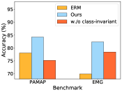
(a) Class-invariant feat.

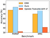
(b) Update feat. with $d^{\prime}$

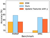
(c) Update feature with $y$

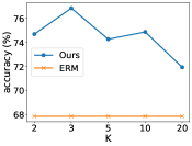
(d) #Domain $K$ (EMG)

Figure 5: Ablation study of Diversify.

We observe more insightful conclusions. (1) When the task is difficult: In the Cross-Person setting, USC-HAD may be the most difficult task. Although it has more samples, it contains 14 subjects with only two sensors on one position, which may bring more difficulty in learning. The results prove the above argument that all methods perform terribly on this benchmark while ours has the largest improvement. (2) When datasets are significantly more diverse: Compared to Cross-Person and Cross-Position settings, Cross-Dataset may be more difficult since all datasets are totally different and samples are influenced by subjects, devices, sensor positions, and some other factors. In this setting, our method is substantially better than others. (3) Limited data: Compared with Cross-Person setting, One-Person-To-Another is more difficult since it has fewer data samples. In this case, enhancing diversity can bring a remarkable improvement and our method can boost the performance.

3.5 Analysis

Ablation study

We present ablation study to answer the following three questions. (1) Why obtaining pseudo domain labels with class-invariant features in step 3? If we obtain pseudo domain labels with common features, domain labels may have correlations with class labels, which may introduce contradictions when learning domain-invariant representations and lead to common performance. This is certified by the results in Figure 5(a). (2) Why using fine-grained domain-class labels in step 2? If we utilize pseudo domain labels to update the feature net, it may make the representations seriously biased towards domain-related features and thereby leads to terrible performance on classification, which is proved in Figure 5(b). If we only utilize class labels to update the feature net, it may make representations biased to class-related features, thus Diversify is unable to obtain true latent sub-domains, as shown in Figure 5(c). Hence, we should employ fine-grained domain-class labels to obtain representations with both domain and class information. (3) The more latent domains, the better? More latent domains may not bring better results (Figure 5(d)) since a dataset may only have a few latent domains and introducing more may contradict its intrinsic data property. Plus, more latent domains also make it harder to obtain pseudo domain labels and learn domain-invariant features.

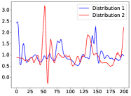
(a) USC-HAD

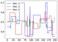
(b) EMG

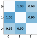
(c) Initial splits

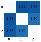
(d) Our splits

Figure 6: (a) (b) Latent distributions obtained by our method on two datasets. X-axis is data numbers while Y-axis is its values. (c) (d) $\mathcal{H}$-divergence among domains with initial splits and our splits on PAMAP. Axes are domain numbers.

 

Existence of latent distributions

What exactly can our Diversify learn? In Figure 6(a), for a subject in USC-HAD, there is more than one latent distribution for his walking activities, showing the existence of temporal distribution shift: the distribution of the same activity could change. For spatial distribution shift, Figure 6(b) on EMG dataset shows that our algorithm found three latent distributions from the EMG data of multiple people. These results indicate the existence of latent distributions with both temporal and spatial distribution shifts. More results are in Appendix F.1.

Quantitative analysis for ‘worst-case’ distributions

We present quantitative analysis by computing the $\mathcal{H}$-divergence (Ben-David et al., 2010) to show the effectiveness of our ‘worst-case distribution’. As shown in Figure 6(c) and 6(d), compared to initial domain splits, latent sub-domains generated by our method have larger $\mathcal{H}$-divergence among each other. According to Prop. 2.1, larger $\mathcal{H}$-divergence among domains brings better generalization. This again shows the efficacy of Diversify in computing the ’worst-case’ distribution scenario. More results are in Appendix F.3.

Visualization study

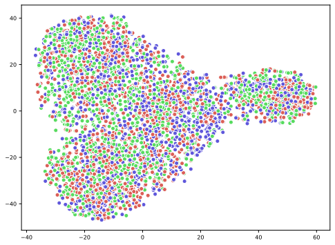
(a) Initial domain split

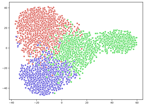
(b) Our domain split

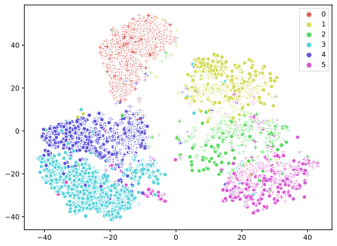
(c) ANDMask

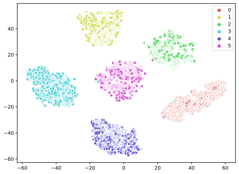
(d) Our classification

Figure 7: t-SNE visualizations for domain splits ((a) (b)) and classification ((c) (d)) on EMG data.

 

We present some visualizations to show the rationales of Diversify. Data points with different initial domain labels are mixed together in Figure 7(a) while Diversify can characterize different latent distributions and separate them well in Figure 7(b). Figure 7(d) and 7(c) show that Diversify can learn better domain-invariant representations compared to the latest method ANDMask. To sum up, Diversify can find better latent domains to enhance generalization. More results are in Appendix F.1.

Varying backbones

Figure 8 shows the results using small, medium, and large backbones, respectively (we implement them with different numbers of layers.). Results indicate that larger models tend to achieve better OOD generalization performance. Our method outperforms others in all backbones, showing that Diversify presents consistently strong OOD performance in different architectures. More results with Transformer are in Appendix F.4 Parameter sensitivity is in Appendix F.2.

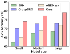
Figure 8: Results with different backbones on EMG.

4 Related Work

Time series classification is a challenging problem. Researches mainly focus on temporal relation modeling via specially-designed methods (Dempster et al., 2021), RNN-based networks (Dennis et al., 2019), or Transformer architecture (Drouin et al., 2022). To our best knowledge, there is only one recent work (Du et al., 2021) that studied time series from the distribution level. However, AdaRNN is a two-stage non-differential method that is tailored for RNN.

Domain / OOD generalization (Wang et al., 2022; Lu et al., 2022) typically assumes the availablality of domain labels for training. Specifically, Matsuura & Harada (2020) also studied DG without domain labels by clustering with the style features for images, which is not applied to time series and is not end-to-end trainable. Disentanglement (Peng et al., 2019; Zhang et al., 2022b) tries to disentangle the domain and label information, but they also assume access to domain information. Single domain generalization is similar to our problem setting that also involves one training domain (Fan et al., 2021; Li et al., 2021; Wang et al., 2021; Zhu & Li, 2022). However, they treated the single domain as one distribution and did not explore latent distributions.

Multi-domain learning is similar to DG which also trains on multiple domains, but also tests on training distributions. Deecke et al. (2022) proposed sparse latent adapters to learn from unknown domain labels, but their work does not consider the min-max worst-case distribution scenario and optimization. In domain adaptation, Wang et al. (2020) proposed the notion of domain index and further used variational models to learn them (Xu et al., 2023), but took different modeling methodology since they did not consider min-max optimization. Mixture models (Rasmussen et al., 1999) are models representing the presence of subpopulations within an overall population, e.g., Gaussian mixture models. Our approach has a similar formulation, but does not use generative models. Subpopulation shift is a new setting (Koh et al., 2021) that refers to the case where the training and test domains overlap, but their relative proportions differ. Our problem does not belong to this setting since we assume that these distributions do not overlap.

Distributionally robust optimization (Delage & Ye, 2010) shares a similar paradigm with our work, whose paradigm is also to seek a distribution that has the worst performance within a range of the raw distribution. GroupDRO (Sagawa et al., 2020) studied DRO at a group level. However, we study the internal distribution shift instead of seeking a global distribution close to the original one.

5 Limitation and Discussion

Diversify could be more perfect by pursuing the following avenues. 1) Estimate the number of latent distributions $K$ automatically: we currently treat it as a hyperparameter. 2) Seek the semantics behind latent distributions (e.g., Figure 6(a)): can adding more human knowledge obtain better latent distributions? 3) Extend Diversify to beyond classification, but for forecasting problems.

Moreover, we argue that dynamic distributions not only exist in time series, but also in general machine learning data such as image and text (Deecke et al., 2022; Xu et al., 2023). Thus, it is of great interest to apply our approach to these domains to further improve their performance.

6 Conclusion

We proposed Diversify to learn generalized representation for time series classification. Diversify employs an adversarial game that maximizes the ‘worst-case’ distribution scenario while minimizing their distribution divergence. We demonstrated its effectiveness in different applications. We are surprised that not only a mixed dataset, but one dataset from a single person can also contain several latent distributions. Characterizing such latent distributions will greatly improve the generalization performance on unseen datasets.

.tocmtappendix mtchapternone mtappendixsubsection

Appendix A Theoretical Insights

A.1 Background

For a distribution $\mathbb{P}$ with an ideal binary labeling function $h^{*}$ and a hypothesis $h$, we define the error $\varepsilon_{\mathbb{P}}(h)$ in accordance with (Ben-David et al., 2010) as:

$$\varepsilon_{\mathbb{P}}(h)=\mathbb{E}_{\mathbf{x}\sim\mathbb{P}}|h(\mathbf{x})-h^{*}(\mathbf{x})|.$$ (9)

We also give the definition of $\mathcal{H}$-divergence according with (Ben-David et al., 2010). Given two distributions $\mathbb{P},\mathbb{Q}$ over a space $\mathcal{X}$ and a hypothesis class $\mathcal{H}$,

$$d_{\mathcal{H}}(\mathbb{P},\mathbb{Q})=2\sup_{h\in\mathcal{H}}|Pr_{\mathbb{P}}(I_{h})-Pr_{\mathbb{Q}}(I_{h})|,$$ (10)

where $I_{h}=\{\mathbf{x}\in\mathcal{X}|h(\mathbf{x})=1\}$. We often consider the $\mathcal{H}\Delta\mathcal{H}$-divergence in (Ben-David et al., 2010) where the symmetric difference hypothesis class $\mathcal{H}\Delta\mathcal{H}$ is the set of functions characteristic to disagreements between hypotheses.

Theorem A.1.

(Theorem 2.1 in (Sicilia et al., 2021), modified from Theorem 2 in (Ben-David et al., 2010)). Let $\mathcal{X}$ be a space and $\mathcal{H}$ be a class of hypotheses corresponding to this space. Suppose $\mathbb{P}$ and $\mathbb{Q}$ are distributions over $\mathcal{X}$. Then for any $h\in\mathcal{H}$, the following holds

$$\varepsilon_{\mathbb{Q}}(h)\leq\lambda^{\prime\prime}+\varepsilon_{\mathbb{P}}(h)+\frac{1}{2}d_{\mathcal{H}\Delta\mathcal{H}}(\mathbb{Q},\mathbb{P})$$ (11)

with $\lambda^{\prime\prime}$ the error of an ideal joint hypothesis for $\mathbb{Q},\mathbb{P}$.

Theorem A.1 provides an upper bound on the target-error. $\lambda^{\prime\prime}$ is a property of the dataset and hypothesis class and is often ignored. Theorem A.1 demonstrates the necessity to learn domain invariant features.

A.2 Proof of Proposition 2.1.

Proposition 2.1.

Let $\mathcal{X}$ be a space and $\mathcal{H}$ be a class of hypotheses corresponding to this space. Let $\mathbb{Q}$ and the collection $\{\mathbb{P}_{i}\}_{i=1}^{K}$ be distributions over $\mathcal{X}$ and let $\{\varphi_{i}\}_{i=1}^{K}$ be a collection of non-negative coefficient with $\sum_{i}\varphi_{i}=1$. Let the object $\mathcal{O}$ be a set of distributions such that for every $\mathbb{S}\in\mathcal{O}$ the following holds

$$d_{\mathcal{H}\Delta\mathcal{H}}(\sum_{i}\varphi_{i}\mathbb{P}_{i},\mathbb{S})\leq\max_{i,j}d_{\mathcal{H}\Delta\mathcal{H}}(\mathbb{P}_{i},\mathbb{P}_{j}).$$ (12)

Then, for any $h\in\mathcal{H}$,

$$\varepsilon_{\mathbb{Q}}(h)\leq\lambda^{\prime}+\sum_{i}\varphi_{i}\varepsilon_{\mathbb{P}_{i}}(h)+\frac{1}{2}\min_{\mathbb{S}\in\mathcal{O}}d_{\mathcal{H}\Delta\mathcal{H}}(\mathbb{S},\mathbb{Q})+\frac{1}{2}\max_{i,j}d_{\mathcal{H}\Delta\mathcal{H}}(\mathbb{P}_{i},\mathbb{P}_{j})$$ (13)

where $\lambda^{\prime}$ is the error of an ideal joint hypothesis.

Proof.

On one hand, with Theorem A.1, we have

$$\varepsilon_{\mathbb{Q}}(h)\leq\lambda^{\prime}_{1}+\varepsilon_{\mathbb{S}}(h)+\frac{1}{2}d_{\mathcal{H}\Delta\mathcal{H}}(\mathbb{S},\mathbb{Q}),\forall h\in\mathcal{H},\forall\mathbb{S}\in\mathcal{O}.$$ (14)

On the other hand, with Theorem A.1, we have

$$\varepsilon_{\mathbb{S}}(h)\leq\lambda^{\prime}_{2}+\varepsilon_{\sum_{i}\varphi_{i}\mathbb{P}_{i}}(h)+\frac{1}{2}d_{\mathcal{H}\Delta\mathcal{H}}(\sum_{i}\varphi_{i}\mathbb{P}_{i},\mathbb{S}),\forall h\in\mathcal{H}.$$ (15)

Since $\varepsilon_{\sum_{i}\varphi_{i}\mathbb{P}_{i}}(h)=\sum_{i}\varphi_{i}\varepsilon_{\mathbb{P}_{i}}(h)$, and $d_{\mathcal{H}\Delta\mathcal{H}}(\sum_{i}\varphi_{i}\mathbb{P}_{i},\mathbb{S})\leq\max_{i,j}d_{\mathcal{H}\Delta\mathcal{H}}(\mathbb{P}_{i},\mathbb{P}_{j})$, we have

$$\varepsilon_{\mathbb{Q}}(h)\leq\lambda^{\prime}+\sum_{i}\varphi_{i}\varepsilon_{\mathbb{P}_{i}}(h)+\frac{1}{2}d_{\mathcal{H}\Delta\mathcal{H}}(\mathbb{S},\mathbb{Q})+\frac{1}{2}\max_{i,j}d_{\mathcal{H}\Delta\mathcal{H}}(\sum_{i}\varphi_{i}\mathbb{P}_{i},\mathbb{S}),\forall h\in\mathcal{H},\forall\mathbb{S}\in\mathcal{O},$$ (16)

where $\lambda^{\prime}=\lambda^{\prime}_{1}+\lambda^{\prime}_{2}$. Equation 16 for all $\mathbb{S}\in\mathcal{O}$ holds. Therefore, we complete the proof. ∎

Appendix B Method Details

B.1 Domain-invariant Representation Learning

Domain-invariant representation learning utilizes adversarial training which contains a feature network, a domain discriminator, and a classification network. The domain discriminator tries its best to discriminate domain labels of data while the feature network tries its best to generate features to confuse the domain discriminator, which thereby obtains domain-invariant representation. Therefore, it is an adversarial process, and in our setting, it can be expressed as follows,

$$\min_{h_{b}^{(4)},h_{c}^{(4)}} \mathbb{E}_{(\mathbf{x},y)\sim\mathbb{P}^{tr}}\ell(h_{c}^{(4)}(h_{b}^{(4)}(h_{f}^{(4)}(\mathbf{x}))),y)-\ell(h_{adv}^{(4)}(h_{b}^{(4)}(h_{f}^{(4)}(\mathbf{x}))),d^{\prime}),$$ (17)

$$\min_{h_{adv}^{(4)}} \mathbb{E}_{(\mathbf{x},y)\sim\mathbb{P}^{tr}}\ell(h_{adv}^{(4)}(h_{b}^{(4)}(h_{f}^{(4)}(\mathbf{x}))),d^{\prime}).$$

To optimize Eq. (17), we need an iterative process to optimize $h_{b}^{(4)},h_{c}^{(4)}$ and $h_{adv}^{(4)}$ iteratively, which is cumbersome. It is better to optimize $h_{b}^{(4)},h_{c}^{(4)}$ and $h_{adv}^{(4)}$ at the same time. It is obvious that the key is to solve the problems caused by the negative sign in Eq. (17). Therefore, a special gradient reversal layer (GRL), a popular implementation of the adversarial training in training several domains as suggested by (Ganin et al., 2016), came. GRL acts as an identity transformation during the forward propagation while it takes the gradient from the subsequent level and changes its sign before passing it to the preceding layer during the backpropagation. During the forward propagation, the GRL can be ignored. During the backpropagation, the GRL makes the sign of gradient on $h_{b}^{(4)}$ reverse, which solves the problems caused by the negative sign in Eq. (17).

B.2 Method Formulation and Implementation

While it is common to use some probability or Bayesian approaches for formulation when one mentions distributions, we actually do not formulate the latent distributions: we are not a generative or parametric method. In fact, the concept of latent distribution is just a notion to help understand our method. Our ultimate goal is to infer which distribution a segment belongs to for best OOD performance. Thus, we do not care what a distribution exactly looks like or even parameterize it since it is not our focus. As long as we can obtain diverse latent distributions, things are all done.

In real implementation, the latent distributions are just represented as domain labels: latent distribution $i$ is also a domain $i$ that certain time series segments belong to, as we stated in the introduction part. Additionally, we also acknowledge that parameterizing the latent distributions may help to get better performance, which can be left for future research.

B.3 Comparisons to Other Latest Methods

Here, we offer more details on comparisons to other latest methods utilized in the main paper.

• DANN (Ganin et al., 2016) is a method that utilizes the adversarial training to force the discriminator unable to classify domains for better domain-invariant features. It requires domain labels and splits data in advance while ours is a universal method.

• CORAL (Sun & Saenko, 2016) is a method that utilizes the covariance alignment in feature layers for better domain-invariant features. It also requires domain labels and splits data in advance.

• Mixup (Zhang et al., 2018) is a method that utilizes interpolation to generate more data for better generalization. Ours mainly focuses on generalized representation learning.

• GroupDRO (Sagawa et al., 2020) is a method that seeks a global distribution with the worst performance within a range of the raw distribution for better generalization. Ours study the internal distribution shift instead of seeking a global distribution close to the original one.

• RSC (Huang et al., 2020) is a self-challenging training algorithm that forces the network to activate features as much as possible by manipulating gradients. It belongs to gradient operation-based DG while ours is to learn generalized features.

• ANDMask (Parascandolo et al., 2021) is another gradient-based optimization method that belongs to special learning strategies. Ours focuses on representation learning.

• GILE (Qian et al., 2021) is a disentanglement method designed for cross-person human activity recognition. It is based on VAEs and requires domain labels.

• AdaRNN (Du et al., 2021) is a method with a two-stage that is non-differential and it is tailored for RNN. A specific algorithm is designed for splitting. Ours is universal and is differential with better performance.

Appendix C Dataset

C.1 Datasets Information

Table 4 shows the statistical information on each dataset.

Table 4: Information on datasets.

Dataset	Subjects	Sensors	Classes	Samples
EMG	36	1	7	33,903,472
SPCMD	2618	-	35	105,829
WESAD	15	8	4	63,000,000
DSADS	8	3	19	1,140,000
USC-HAD	14	2	12	5,441,000
UCI-HAR	30	2	6	1,310,000
PAMAP	9	3	18	3,850,505

C.2 More details on EMG

Electromyography (EMG) is a typical time-series data that is based on bioelectric signals. We use EMG for gestures Data Set (Lobov et al., 2018) that contains raw EMG data recorded by MYO Thalmic bracelet. The bracelet is equipped with eight sensors equally spaced around the forearm that simultaneously acquire myographic signals. Data of 36 subjects are collected while they performed series of static hand gestures and the number of instances is $~{}40,000-50,000$ recordings in each column. It contains 7 classes and we select 6 common classes for our experiments. We randomly divide 36 subjects into four domains (i.e., $0,1,2,3$) without overlapping and each domain contains data of 9 persons.

C.3 Details on Sensor-based Human Activity Recognition Dataset

UCI daily and sports dataset (DSADS) (Barshan & Yüksek, 2014) consists of 19 activities collected from 8 subjects wearing body-worn sensors on 5 body parts. USC-SIPI human activity dataset (USC-HAD) (Zhang & Sawchuk, 2012) is composed of 14 subjects (7 male, 7 female, aged 21 to 49) executing 12 activities with a sensor tied on the front right hip. UCI-HAR (Anguita et al., 2012) is collected by 30 subjects performing 6 daily living activities with a waist-mounted smartphone. PAMAP (Reiss & Stricker, 2012) contains data of 18 activities, performed by 9 subjects wearing 3 sensors.

C.4 Details on Different Settings for Human Activity Recognition

We construct four different settings representing different degrees of generalization: (1) Cross-person generalization: This setting utilizes DSADS, USC-HAD, PAMAP datasets to construct three benchmarks. Within each dataset, we randomly split the data into four groups and then use three groups as training data to learn a generalized model for the last group. (2) Cross-position generalization: this setting uses DSADS dataset and data from each position denotes a different domain. Each sample contains three sensors with nine dimensions. We treat one position as the test domain while the others are for training. (3) Cross-dataset generalization: this setting uses all four datasets, and each dataset corresponds to a different domain. Six common classes are selected. Two sensors from each dataset that belong to the same position are selected and data is down-sampled to have the same dimension. (4) One-Person-To-Another. This setting adopts DSADS, USC-HAD, and PAMAP datasets. In each dataset, we randomly select four pairs of persons where one is the training and the other is the test.

C.5 Data Preprocessing

We will introduce how we preprocess data and the final dimension of data for experiments here. We mainly utilize the sliding window technique, a common technique in time-series classification, to split data. As its name suggests, this technique involves taking a subset of data from a given array or sequence. Two main parameters of the sliding window technique are the window size, describing a subset length, and the step size, describing moving forward distance each time.

For EMG, we set the window size 200 and the step size 100, which means there exist $50\%$ overlaps between two adjacent samples. We normalize each sample with $\tilde{\mathbf{x}}=\frac{\mathbf{x}-\min\mathbf{X}}{\max\mathbf{X}-\min\mathbf{X}}$. $\mathbf{X}$ contains all $\mathbf{x}$. The final dimension is $8\times 1\times 200$.

For Speech Commands, we follow (Kidger et al., 2020).

For WESAD, we utilize the same preprocessing as EMG.

Now we give details on all datasets in Cross-person setting. For DSADS, we directly utilize data split by the providers. The final dimension shape is $45\times 1\times 125$. $45=5\times 3\times 3$ where $5$ means five positions, the first $3$ means three sensors, and the second $3$ means each sensor has three axes. For USC-HAD, the window size is 200 and the step size is 100. The final dimension shape is $6\times 1\times 200$. For PAMAP, the window size is 200 and the step size is 100. The final dimension shape is $27\times 1\times 200$. For UCI-HAR, we directly utilize data split by the providers. The final dimension shape is $6\times 1\times 128$.

For Cross-position, we directly utilize samples obtained from DSADS in Cross-person setting. Since each position corresponds to one domain, a sample is split into five samples in the first dimension. And the final dimension shape is $9\times 1\times 125$.

For Cross-dataset, we directly utilize samples obtained in Cross-person setting. To make all datasets share the same label space and input space, we select six common classes, including WALKING, WALKING UPSTAIRS, WALKING DOWNSTAIRS, SITTING, STANDING, LAYING. In addition, we down-sample data and select two sensors from each dataset that belong to the same position. The final dimension shape is $6\times 1\times 50$.

For One-Person-To-Another, we randomly select four pairs of persons from DSADS, USC-HAD, and PAMAP respectively. Four tasks are $1\rightarrow 0,3\rightarrow 2,5\rightarrow 4,$ and $7\rightarrow 6$. Each number corresponds to one subject. And the final dimension shape is $45\times 1\times 125,6\times 1\times 200,$ and $27\times 1\times 200$ for DSADS, USC-HAD, and PAMAP respectively.

As we can see, samples in EMG, WESAD, and HAR all have more than one channel (the first dimension shape), which means they are all multivariate.

C.6 Details on Domain Splits

We introduce how we split data here.

Since Speech Commands is a regular task, we just randomly split the entire dataset into a training dataset, a validation dataset, and a testing dataset.

We mainly focus on EMG, WESAD, and HAR, and we construct domains for OOD tasks. We denote subjects of a dataset with $0-s_{n}$, where $s_{n}$ is the number of subjects in the dataset. For example, there are 36 subjects in EMG and we utilize $0,1,2,\cdots,35$ to denote data of them respectively.

Table 5 shows the initial domain splits of EMG, WESAD, and all datasets for HAR in Cross-person setting. We just want to make each domain has a similar number of samples in one dataset. As noted in the main paper, we also utilize 0, 1, 2, and 3 to represent different domains but they have different meanings with subjects. When conducting experiments, we take one domain as the testing data and the others as the training data. Our method is not influenced by the splits of the training data since we do not need the domain labels.

Table 5: Initial domain splits.

Dataset	0	1	2	3
EMG	0-8	9-17	18-26	27-35
WESAD	0-3	4-7	8-11	12-14
DSADS	0,1	2,3	4,5	6,7
USC-HAD	0,1,2,11	3,5,6,9	7,8,10,13	4,12
PAMAP	2,3,8	1,5	0,7	4,6

Appendix D Network Architecture and Hyperparameters

For the architecture, the model contains two blocks, and each has one convolution layer, one pooling layer, and one batch normalization layer. A single-fully-connected layer is used as the bottleneck layer while another fully-connected layer serves as the classifier. All methods are implemented with PyTorch (Paszke et al., 2019). The maximum training epoch is set to 150. The Adam optimizer with weight decay $5\times 10^{-4}$ is used. The learning rate for GILE is $10^{-4}$. The learning rate for the rest methods is $10^{-2}$ or $10^{-3}$. (For Speech Commands with MatchBoxNet3-1-64, we also try the learning rate, $10^{-4}$.) We tune hyperparameters for each method.

For the pooling layer, we utilize MaxPool2d in PyTorch. The kernel size is $(1,2)$ ad the stride is 2. For the convolution layer, we utilize Conv2d in PyTorch. Different tasks have different kernel sizes and Table 6 shows the kernel sizes.

Table 6: The kernel size of each benchmark.

EMG	(1,9)	Cross-Person	DSADS	(1,9)
SPEECHCOMMANDS	(1,9)		USC-HAD	(1,6)
WESAD	(1,9)		PAMAP2	(1,9)
Cross-position	(1,9)	One-Person-To-Another	The same as Cross-Person
Cross-dataset	(1,6)

Appendix E Evaluation Metrics

We utilize average accuracy on the testing dataset as our evaluation metrics for all benchmarks. Average accuracy is the most common metric for DG and it can be computed as the following,

$$Acc=\frac{\sum_{(\mathbf{x},y)\in\mathcal{D}^{te}}I_{y}(y*)}{\#|\mathcal{Y}^{te}|},$$ (18)

$$y*=\arg\max h(\mathbf{x}).$$

$I_{y}(y*)$ is an indicator function. If $y=y*$, it equals 1, otherwise it equals 0. $\#|\cdot|$ represents the number of the set. $h$ is the model to learn. Please note that $\mathcal{X}^{te}$ has a different distribution from $\mathcal{X}^{tr}$ for EMG and HAR. And $\mathbf{x}$ has been preprocessed and each sample is a segment.

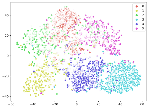
(a) ERM

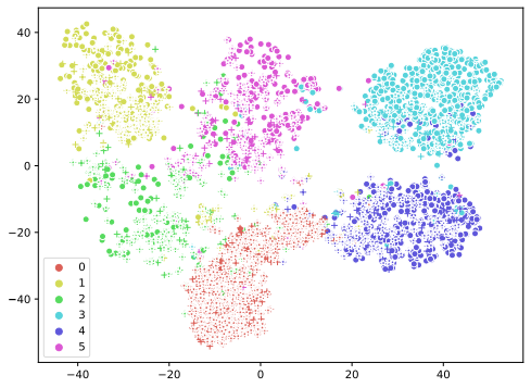
(b) RSC

(c) ANDMask

(d) Ours

Figure 9: Visualization of the t-SNE embeddings for classification on EMG. Different colors correspond to different classes while different shapes correspond to different domains.

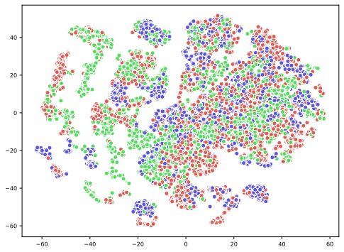
(a) Initial splits on USC

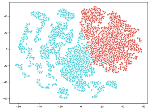
(b) Our splits on USC

(c) Initial splits on EMG

(d) Our splits on EMG

Figure 10: Visualization of the t-SNE embeddings for domain splits where different colors represent different domains.

Appendix F More Experimental Results

F.1 Visualization Study

We show more visualization study in this part. As shown in Figure 9(a) and Figure 9(b), both ERM and RSC also cannot obtain fine domain-invariant representations and our method still achieves the best domain-invariant representations. As shown in Figure 10, compared with initial domain splits, latent sub-domains generated by our method are better separated.

F.2 Parameter Sensitivity

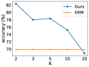
(a) #Latent domains $K$

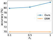
(b) $\lambda_{1}$

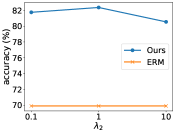
(c) $\lambda_{2}$

(d) Local epoch and Round

Figure 11: Parameter sensitivity analysis (EMG).

There are mainly four hyperparameters in our method: $K$ which is the number of latent sub-domains, $\lambda_{1}$ for the adversarial part in step 3, $\lambda_{2}$ for the adversarial part in step 4, and local epochs and total rounds. For fairness, the product of local epochs and total rounds is the same value. We evaluate the parameter sensitivity of our method in Figure 11 where we change one parameter and fix the other to record the results. From these results, we can see that our method achieves better performance in a wide range, demonstrating that our method is robust.

F.3 $\mathcal{H}$-divergence

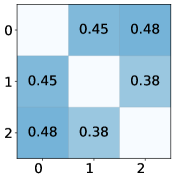
(a) Initial splits

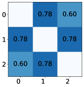
(b) Our splits

Figure 12: $\mathcal{H}$-divergence among domains with initial splits and our splits on EMG.

Figure 12 shows $\mathcal{H}$-divergence among domains with initial splits and our splits on EMG, which demonstrates our splits have larger $\mathcal{H}$-divergence and thereby can bring better generalization.

F.4 The Influence of Architectures

Table 7: Results on EMG dataset with different model sizes.

Model Size	Small					Medium					Large
Target	0	1	2	3	AVG	0	1	2	3	AVG	0	1	2	3	AVG
ERM	56.6	65.7	65.3	61.8	62.3	62.6	69.9	67.9	69.3	67.4	61.2	78.8	68.8	64.6	68.4
DANN	65.3	69.3	63.6	62.9	65.3	62.9	70.0	66.5	68.2	66.9	63.0	72.7	69.4	68.5	68.4
CORAL	66.9	74.9	70.8	73.2	71.4	66.4	74.6	71.4	74.2	71.7	67.7	77.0	72.7	71.8	72.3
Mixup	56.8	61.0	68.1	67.2	63.2	60.7	69.9	70.5	68.2	67.3	66.3	81.1	71.2	69.6	72.0
GroupDRO	64.9	75.0	71.6	69.1	70.1	67.6	77.5	73.7	72.5	72.8	66.3	79.3	74.9	71.3	73.0
RSC	62.7	73.2	67.6	64.0	66.9	70.1	74.6	72.4	71.9	72.2	65.1	76.8	72.2	67.7	70.4
ANDMask	62.4	66.0	66.3	65.6	65.1	66.6	69.1	71.4	68.9	69.0	65.7	78.1	72.1	71.9	71.9
DIVERSIFY	69.8	77.3	74.4	74.4	74.0	71.7	82.4	76.9	77.3	77.1	72.0	86.6	78.5	78.9	79.0

To ensure that our method can work with different sizes of models, we add some more experiments with more complex or simpler architectures. As shown in Table 7, where small, medium, and large indicate the different model sizes (our paper uses the medium), we see a clear picture that model sizes influence the results, and our method also achieves the best performance. Small corresponds to the model with one convolutional layer, Medium corresponds to the model with two convolutional layers, and Large corresponds to the model with four convolutional layers. For most methods, more complex models bring better results.

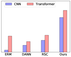
Figure 13: Results on the first task in Cross-dataset generalization using Transformers.

We also try Transformer (Vaswani et al., 2017) as the backbone for comparisons. As shown in (Zhang et al., 2022a), Transformer often has a better generalization ability compared to CNN, which implies improving with Transformer is more difficult. From Table 8, we can see that each method with Transformer has a remarkable improvement on EMG. Compared to ERM, DANN almost has no improvement but ours still has further improvements and achieves the best performance. To further validate the advantage of our method, we perform the experiments on a more difficult task, i.e. the first task of cross-dataset where distribution gaps are larger. As shown in Figure 13, our method still achieves the best performance in this more difficult situation while DANN even performs worse than ERM, which demonstrates the importance of more accurate sub-domain labels.

Table 8: Results on EMG dataset with Transformer.

Target	0	1	2	3	AVG
ERM	71.7	83.8	76.1	78.0	77.4
DANN	72.7	82.3	77.6	77.3	77.5
GroupDRO	72.1	84.4	77.5	78.3	78.1
RSC	72.1	83.7	77.6	78.2	77.9
Ours	75.6	86.2	79.4	79.7	80.2

Overall, for all architectures, our method achieves the best performance.

Table 9: Time costs of different methods (s).

method	ERM	DANN	CORAL	Mixup	GroupDRO	RSC	ANDMask	Ours
time	305.98	328.62	357.54	2042.93	340.03	321.51	379.87	356.8

F.5 Time Complexity and Convergence Analysis

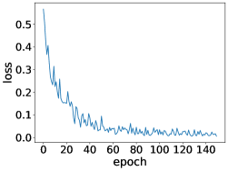
Figure 14: Convergence results on EMG.

We also provide some analysis on time complexity and convergence. Since we only optimize the feature extractor in Step 2, our method does not cost too much time. And the results in Table 9 prove this argument empirically.

The convergence results are shown in Figure 14. Our method is convergent. Although there are some little fluctuations, these fluctuations exist widely in all domain generalization methods due to different distributions of different samples.

References

- Anguita et al. (2012) Davide Anguita, Alessandro Ghio, Luca Oneto, Xavier Parra, and Jorge L Reyes-Ortiz. Human activity recognition on smartphones using a multiclass hardware-friendly support vector machine. In International workshop on ambient assisted living, pp. 216–223. Springer, 2012.
- Barshan & Yüksek (2014) Billur Barshan and Murat Cihan Yüksek. Recognizing daily and sports activities in two open source machine learning environments using body-worn sensor units. The Computer Journal, 57(11):1649–1667, 2014.
- Ben-David et al. (2010) Shai Ben-David, John Blitzer, Koby Crammer, Alex Kulesza, Fernando Pereira, and Jennifer Wortman Vaughan. A theory of learning from different domains. Machine learning, 79(1):151–175, 2010.
- Caron et al. (2018) Mathilde Caron, Piotr Bojanowski, Armand Joulin, and Matthijs Douze. Deep clustering for unsupervised learning of visual features. In Proceedings of the European Conference on Computer Vision (ECCV), pp. 132–149, 2018.
- Das et al. (1998) Gautam Das, King-Ip Lin, Heikki Mannila, Gopal Renganathan, and Padhraic Smyth. Rule discovery from time series. In KDD, volume 98, pp. 16–22, 1998.
- Deecke et al. (2022) Lucas Deecke, Timothy Hospedales, and Hakan Bilen. Visual representation learning over latent domains. In International Conference on Learning Representations, 2022.
- Delage & Ye (2010) Erick Delage and Yinyu Ye. Distributionally robust optimization under moment uncertainty with application to data-driven problems. Operations research, 58(3):595–612, 2010.
- Dempster et al. (2021) Angus Dempster, Daniel F Schmidt, and Geoffrey I Webb. Minirocket: A very fast (almost) deterministic transform for time series classification. In Proceedings of the 27th ACM SIGKDD conference on knowledge discovery & data mining, pp. 248–257, 2021.
- Dennis et al. (2019) Don Dennis, Durmus Alp Emre Acar, Vikram Mandikal, Vinu Sankar Sadasivan, Venkatesh Saligrama, Harsha Vardhan Simhadri, and Prateek Jain. Shallow rnn: accurate time-series classification on resource constrained devices. Advances in Neural Information Processing Systems, 32, 2019.
- Drouin et al. (2022) Alexandre Drouin, Étienne Marcotte, and Nicolas Chapados. Tactis: Transformer-attentional copulas for time series. In International Conference on Machine Learning, ICML, volume 162, pp. 5447–5493, 2022.
- Du et al. (2021) Yuntao Du, Jindong Wang, Wenjie Feng, Sinno Pan, Tao Qin, Renjun Xu, and Chongjun Wang. Adarnn: Adaptive learning and forecasting of time series. In Proceedings of the 30th ACM International Conference on Information & Knowledge Management, pp. 402–411, 2021.
- Fan et al. (2021) Xinjie Fan, Qifei Wang, Junjie Ke, Feng Yang, Boqing Gong, and Mingyuan Zhou. Adversarially adaptive normalization for single domain generalization. In Proceedings of the IEEE/CVF Conference on Computer Vision and Pattern Recognition, pp. 8208–8217, 2021.
- Fawaz et al. (2019) Hassan Ismail Fawaz, Germain Forestier, Jonathan Weber, Lhassane Idoumghar, and Pierre-Alain Muller. Deep learning for time series classification: a review. Data mining and knowledge discovery, 33(4):917–963, 2019.
- Fulcher & Jones (2014) Ben D Fulcher and Nick S Jones. Highly comparative feature-based time-series classification. IEEE Transactions on Knowledge and Data Engineering, 26(12):3026–3037, 2014.
- Ganin et al. (2016) Yaroslav Ganin, Evgeniya Ustinova, Hana Ajakan, Pascal Germain, Hugo Larochelle, François Laviolette, Mario Marchand, and Victor Lempitsky. Domain-adversarial training of neural networks. The journal of machine learning research, 17(1):2096–2030, 2016.
- Gulrajani & Lopez-Paz (2021) Ishaan Gulrajani and David Lopez-Paz. In search of lost domain generalization. In International Conference on Learning Representations, 2021.
- Huang et al. (2020) Zeyi Huang, Haohan Wang, Eric P Xing, and Dong Huang. Self-challenging improves cross-domain generalization. In ECCV, pp. 124–140, 2020.
- Hüsken & Stagge (2003) Michael Hüsken and Peter Stagge. Recurrent neural networks for time series classification. Neurocomputing, 50:223–235, 2003.
- Kidger et al. (2020) Patrick Kidger, James Morrill, James Foster, and Terry Lyons. Neural Controlled Differential Equations for Irregular Time Series. Advances in Neural Information Processing Systems, 2020.
- Koh et al. (2021) Pang Wei Koh, Shiori Sagawa, Sang Michael Xie, Marvin Zhang, Akshay Balsubramani, et al. Wilds: A benchmark of in-the-wild distribution shifts. In ICML, pp. 5637–5664, 2021.
- Krueger et al. (2021) David Krueger, Ethan Caballero, Joern-Henrik Jacobsen, Amy Zhang, Jonathan Binas, Dinghuai Zhang, Remi Le Priol, and Aaron Courville. Out-of-distribution generalization via risk extrapolation (rex). In International Conference on Machine Learning, pp. 5815–5826. PMLR, 2021.
- Li et al. (2021) Lei Li, Ke Gao, Juan Cao, Ziyao Huang, Yepeng Weng, Xiaoyue Mi, Zhengze Yu, Xiaoya Li, and Boyang Xia. Progressive domain expansion network for single domain generalization. In Proceedings of the IEEE/CVF Conference on Computer Vision and Pattern Recognition, pp. 224–233, 2021.
- Li et al. (2019) Shiyang Li, Xiaoyong Jin, Yao Xuan, Xiyou Zhou, Wenhu Chen, Yu-Xiang Wang, and Xifeng Yan. Enhancing the locality and breaking the memory bottleneck of transformer on time series forecasting. Advances in Neural Information Processing Systems, 32:5243–5253, 2019.
- Lobov et al. (2018) Sergey Lobov, Nadia Krilova, Innokentiy Kastalskiy, Victor Kazantsev, and Valeri A Makarov. Latent factors limiting the performance of semg-interfaces. Sensors, 18(4):1122, 2018.
- Lu et al. (2022) Wang Lu, Jindong Wang, Haoliang Li, Yiqiang Chen, and Xing Xie. Domain-invariant feature exploration for domain generalization. Transactions on Machine Learning Research (TMLR), 2022.
- Majumdar & Ginsburg (2020) Somshubra Majumdar and Boris Ginsburg. Matchboxnet: 1d time-channel separable convolutional neural network architecture for speech commands recognition. In Interspeech 2020, 21st Annual Conference of the International Speech Communication Association, Virtual Event, Shanghai, China, 25-29 October 2020, pp. 3356–3360. ISCA, 2020. doi: 10.21437/Interspeech.2020-1058.
- Matsuura & Harada (2020) Toshihiko Matsuura and Tatsuya Harada. Domain generalization using a mixture of multiple latent domains. In AAAI, 2020.
- Parascandolo et al. (2021) Giambattista Parascandolo, Alexander Neitz, Antonio Orvieto, Luigi Gresele, and Bernhard Schölkopf. Learning explanations that are hard to vary. In ICLR, 2021.
- Paszke et al. (2019) Adam Paszke, Sam Gross, Francisco Massa, Adam Lerer, James Bradbury, Gregory Chanan, Trevor Killeen, Zeming Lin, Natalia Gimelshein, Luca Antiga, et al. Pytorch: An imperative style, high-performance deep learning library. volume 32, pp. 8026–8037, 2019.
- Peng et al. (2019) Xingchao Peng, Zijun Huang, Ximeng Sun, and Kate Saenko. Domain agnostic learning with disentangled representations. In International Conference on Machine Learning, pp. 5102–5112. PMLR, 2019.
- Purushotham et al. (2016) Sanjay Purushotham, Wilka Carvalho, Tanachat Nilanon, and Yan Liu. Variational recurrent adversarial deep domain adaptation. 2016.
- Qian et al. (2021) Hangwei Qian, Sinno Jialin Pan, Chunyan Miao, H Qian, SJ Pan, and C Miao. Latent independent excitation for generalizable sensor-based cross-person activity recognition. In Proceedings of the AAAI Conference on Artificial Intelligence, volume 35, pp. 11921–11929, 2021.
- Ragab et al. (2022) Mohamed Ragab, Zhenghua Chen, Wenyu Zhang, Emadeldeen Eldele, Min Wu, Chee-Keong Kwoh, and Xiaoli Li. Conditional contrastive domain generalization for fault diagnosis. IEEE Transactions on Instrumentation and Measurement, 71:1–12, 2022.
- Rame et al. (2022) Alexandre Rame, Corentin Dancette, and Matthieu Cord. Fishr: Invariant gradient variances for out-of-distribution generalization. In International Conference on Machine Learning, pp. 18347–18377, 2022.
- Rasmussen et al. (1999) Carl Edward Rasmussen et al. The infinite gaussian mixture model. In NIPS, volume 12, pp. 554–560. Citeseer, 1999.
- Reiss & Stricker (2012) Attila Reiss and Didier Stricker. Introducing a new benchmarked dataset for activity monitoring. In 2012 16th international symposium on wearable computers, pp. 108–109. IEEE, 2012.
- Sagawa et al. (2020) Shiori Sagawa, Pang Wei Koh, Tatsunori B Hashimoto, and Percy Liang. Distributionally robust neural networks for group shifts: On the importance of regularization for worst-case generalization. In International Conference on Learning Representations (ICLR), 2020.
- Schmidt et al. (2018) Philip Schmidt, Attila Reiss, Robert Duerichen, Claus Marberger, and Kristof Van Laerhoven. Introducing wesad, a multimodal dataset for wearable stress and affect detection. In Proceedings of the 20th ACM international conference on multimodal interaction, pp. 400–408, 2018.
- Sicilia et al. (2021) Anthony Sicilia, Xingchen Zhao, and Seong Jae Hwang. Domain adversarial neural networks for domain generalization: When it works and how to improve. arXiv preprint arXiv:2102.03924, 2021.
- Sun & Saenko (2016) Baochen Sun and Kate Saenko. Deep coral: Correlation alignment for deep domain adaptation. In European conference on computer vision, pp. 443–450. Springer, 2016.
- Vaswani et al. (2017) Ashish Vaswani, Noam Shazeer, Niki Parmar, Jakob Uszkoreit, Llion Jones, Aidan N Gomez, Łukasz Kaiser, and Illia Polosukhin. Attention is all you need. Advances in neural information processing systems, 30, 2017.
- Wang et al. (2020) Hao Wang, Hao He, and Dina Katabi. Continuously indexed domain adaptation. arXiv preprint arXiv:2007.01807, 2020.
- Wang et al. (2019) Jindong Wang, Yiqiang Chen, Shuji Hao, Xiaohui Peng, and Lisha Hu. Deep learning for sensor-based activity recognition: A survey. Pattern recognition letters, 119:3–11, 2019.
- Wang et al. (2022) Jindong Wang, Cuiling Lan, Chang Liu, Yidong Ouyang, Wenjun Zeng, and Tao Qin. Generalizing to unseen domains: A survey on domain generalization. IEEE Transactions on Knowledge and Data Engineering (TKDE), 2022.
- Wang et al. (2021) Zijian Wang, Yadan Luo, Ruihong Qiu, Zi Huang, and Mahsa Baktashmotlagh. Learning to diversify for single domain generalization. In ICCV, 2021.
- Warden (2018) Pete Warden. Speech commands: A dataset for limited-vocabulary speech recognition. arXiv preprint arXiv:1804.03209, 2018.
- Wilson et al. (2020) Garrett Wilson, Janardhan Rao Doppa, and Diane J Cook. Multi-source deep domain adaptation with weak supervision for time-series sensor data. In Proceedings of the 26th ACM SIGKDD International Conference on Knowledge Discovery & Data Mining, pp. 1768–1778, 2020.
- Xu et al. (2023) Zihao Xu, Guang-Yuan Hao, Hao He, and Hao Wang. Domain-indexing variational bayes: Interpretable domain index for domain adaptation. arXiv preprint arXiv:2302.02561, 2023.
- Zhang et al. (2022a) Chongzhi Zhang, Mingyuan Zhang, Shanghang Zhang, Daisheng Jin, Qiang Zhou, Zhongang Cai, Haiyu Zhao, Xianglong Liu, and Ziwei Liu. Delving deep into the generalization of vision transformers under distribution shifts. In Proceedings of the IEEE/CVF Conference on Computer Vision and Pattern Recognition, pp. 7277–7286, 2022a.
- Zhang et al. (2022b) Hanlin Zhang, Yi-Fan Zhang, Weiyang Liu, Adrian Weller, Bernhard Schölkopf, and Eric P Xing. Towards principled disentanglement for domain generalization. In Proceedings of the IEEE/CVF Conference on Computer Vision and Pattern Recognition, pp. 8024–8034, 2022b.
- Zhang et al. (2018) Hongyi Zhang, Moustapha Cisse, Yann N Dauphin, and David Lopez-Paz. mixup: Beyond empirical risk minimization. In International Conference on Learning Representations, 2018.
- Zhang & Sawchuk (2012) Mi Zhang and Alexander A Sawchuk. Usc-had: a daily activity dataset for ubiquitous activity recognition using wearable sensors. In Proceedings of the 2012 ACM conference on ubiquitous computing, pp. 1036–1043, 2012.
- Zhang et al. (2021) Wenyu Zhang, Mohamed Ragab, and Ramon Sagarna. Robust domain-free domain generalization with class-aware alignment. In ICASSP 2021-2021 IEEE International Conference on Acoustics, Speech and Signal Processing (ICASSP), pp. 2870–2874. IEEE, 2021.
- Zhu & Li (2022) Ronghang Zhu and Sheng Li. Crossmatch: Cross-classifier consistency regularization for open-set single domain generalization. In International Conference on Learning Representations, 2022.
.tocmtappendix \etocsettagdepthmtchapternone \etocsettagdepthmtappendixsubsection