Cold-Start Data Selection for Few-shot Language Model Fine-tuning:
A Prompt-Based Uncertainty Propagation Approach

Abstract

Large Language Models have exhibited remarkable few-shot performance; however, this performance can be sensitive to the selection of few-shot instances. We introduce Patron, a prompt-based data selection method for fine-tuning pre-trained language models under cold-start scenarios, where no initial labeled data are available. In Patron, we develop (1) a prompt-based uncertainty propagation approach for estimating the importance of data points, and (2) a partition-then-rewrite (PTR) strategy to enhance sample diversity when requesting annotations. Experiments conducted on six text classification datasets demonstrate that Patron surpasses the most competitive cold-start data selection baselines by up to 6.9%. Furthermore, with only 128 labels, Patron achieves 91.0% and 92.1% of the fully supervised performance based on conventional fine-tuning and prompt-based learning, respectively. Our implementation of Patron is available at https://github.com/yueyu1030/Patron.

1 Introduction

Pre-trained language models (PLMs) Devlin et al. (2019); Liu et al. (2019); Raffel et al. (2020) have achieved competitive performance with limited labeled data Gao et al. (2021a); Schick and Schütze (2021a, b) for many natural language processing (NLP) tasks. However, there still exists a non-negligible gap between the performance of few-shot and fully-supervised PLMs. Besides, when the task-specific data for fine-tuning is small, the performance of PLMs can have high variance Bragg et al. (2021). As illustrated in Figure 1, when fine-tuning RoBERTa-base Liu et al. (2019) on different subsets of AG News dataset with 32 labels, the performance on the test set varies up to 10% for vanilla fine-tuning and 5% for prompt-based learning Gao et al. (2021a). Such large variations demonstrate the crucial need for strategical selection of training data to improve PLMs’ performance under low-data regimes.

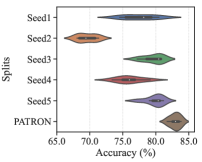
(a) Fine-tuning

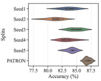
(b) Prompt-based Learning

Figure 1: The performance with large variances of vanilla fine-tuning and prompt-based learning on 5 random samplings, compared with better performance with low variances of Patron (our proposed selection strategy) on AG News Zhang et al. (2015) with 32 labels.

To solicit training data intelligently, active learning (AL) Settles (2011) has been proposed to adaptively annotate unlabeled data Ash et al. (2020); Ein-Dor et al. (2020); Zhang and Plank (2021); Margatina et al. (2021, 2022). Despite their efficacy, most of these works assume there are hundreds, or even thousands of labels in the initial stage, and query similarly significant amounts of labeled data in each AL round. In practice, however, we usually do not have any startup labels to initialize the AL process, and the labeling budget can also be limited. This hinders the application of such techniques, as they often rely on a well-trained model with decent uncertainty Margatina et al. (2021), or gradient estimations Ash et al. (2020) to perform well.

To facilitate training instance selection on such a challenging low-data regime, cold-start data selection (also known as cold-start AL Yuan et al. (2020)) has been proposed, where we have only unlabeled data and zero initial labels, and need to design acquisition functions to effectively query samples for PLM fine-tuning with few labels only.

However, cold-start data selection can be nontrivial for PLMs. Due to the absence of labeled data, the estimated uncertainty for unlabeled data from the PLM can be biased over classes Zhao et al. (2021). As a result, uncertainty-based approaches can underperform even the random selection strategy Hacohen et al. (2022). Moreover, cold-start data selection requires greater care to ensure the sample diversity compared to the traditional AL, as fine-tuning PLMs on few redundant data will lead to poor generalization. Existing approaches often first cluster the whole unlabeled data, and then greedily select samples from each cluster with the predefined heuristics Müller et al. (2022), which fails to control the distance between selected samples and thus cannot fully promote sample diversity. In addition, under cold-start scenarios, it is critical to harness the knowledge from PLMs for sample selection. While there are several methods that leverage pre-trained embeddings Hacohen et al. (2022); Chang et al. (2021) or masked language modeling (MLM) loss (Yuan et al., 2020) to assist data selection, the mismatch between pre-training and fine-tuning tasks hurts their efficacy. To sum up, it is still challenging to design effective methods for cold-start data selection with PLMs.

We propose Patron, a prompt-based data-selection strategy tailored for PLMs, to address the above challenges. To estimate model uncertainty without access to any labeled data under the cold-start setting, Patron leverages prompts Gao et al. (2021a), which convert the classification task into a cloze-style task with customized templates and verbalizers, to generate the task-aware pseudo labels for unlabeled data by predicting the surface name for the [MASK] token. In this way, we also bridge the gap between pre-training and downsteam tasks, and distill task-specific knowledge from PLMs to facilitate data selection.

However, one important issue for such pseudo labels is they can be inaccurate and biased even after calibration Zhao et al. (2021). To remedy this, we further propose uncertainty propagation to first measure the correlation between samples based on kernel similarity in the embedding space, and then propagate their prediction uncertainty to their neighbors. Thus, a sample will have higher propagated uncertainty only when the predictive uncertainty for both itself and its neighbors are high, indicating the model is less certain for the local region around this sample.

To select a batch of diverse samples, we go beyond existing techniques and propose a two stage method named partition-then-rewrite (Ptr), which is initially proposed for combinatorial optimization Chen and Tian (2019), to dynamically adjust the selected sample within each cluster. Concretely, we first use K-Means clustering to partition the unlabeled data and select one sample from each cluster to initialize our solution. We then build a neighbor graph based on $k$-nearest-neighbor (kNN) to encode the neighborhood relationships among selected data and explicitly control the distances between them. After that, we add an additional regularization term to prevent the selected sample in each cluster from being too close to samples in its neighbor clusters. We iterate the above process for several rounds to gradually refine our solution and promote diversity in data selection.

It is worth noting that Patron can be naturally applied to various setups including vanilla fine-tuning, prompt-based learning, semi-supervised learning and standard multi-round AL to improve the data efficiency for PLM fine-tuning. We summarize the key contributions of our work as follows: (1) a cold-start data selection paradigm Patron for lifting the label scarcity issue for few-shot PLM fine-tuning; (2) an prompt-based uncertainty propagation approach to query most informative samples; (3) a partition-then-rewrite (Ptr) strategy to balance between diversity and informativeness of queried samples during AL and (4) experiments on six datasets demonstrating Patron improves the label efficiency over existing baselines by 3.2%–6.9% on average.

2 Related Work

Few-shot Language Model Fine-tuning. Our method is closely relevant to other label-efficient learning paradigms in NLP such as cold-start fine-tuning Zhang et al. (2020b); Shnarch et al. (2022), prompt-based learning Gao et al. (2021a); Schick and Schütze (2021a, b); Min et al. (2022); Zhang et al. (2022c); Hu et al. (2022), semi-supervised learning Du et al. (2021); Wang et al. (2021b); Xie et al. (2020); Xu et al. (2023) and many others, but—orthogonal to our approach—they assume a small set of labeled data is given and design better training strategies. Instead, we aim to select most valuable instances from the unlabeled corpus, which is orthogonal to and can be combined with the above methods to further enhance label efficiency, as shown in Section 5.2 and 5.3.

Training Data Selection. Designing better strategies to selectively annotate training data is not a new research topic. One of the most important line of research lies in active learning (Zhang et al., 2020a; Schröder et al., 2022; Yu et al., 2022), which improves the label efficiency of deep NLP models. However, most of them need a large amount of clean labels to first train the model before data selections Ash et al. (2020); Zhang and Plank (2021). Differently, we aim to facilitate training data selection with minimal supervision, where no initial labeled data is given.

The idea of such cold-start data selection has been applied for image classification Wang et al. (2021a); Hacohen et al. (2022) and speech processing Park et al. (2022), but has not been fully explored for the NLP domain. For this setting, Chang et al. (2021) focus on data selection from the embedding space, but fail to leverage the task-specific knowledge from PLMs. Yuan et al. (2020) uses the MLM loss as a proxy for uncertainty measurement, and Liu et al. (2021a); Su et al. (2022) study few-shot sample selection for billion-scale language models Brown et al. (2020), but mainly focus on in-context learning. Different from the above methods, we aim to leverage prompts to facilitate sample selection, and design additional techniques (i.e., uncertainty propagation and Ptr) to boost the performance of few-shot PLM fine-tuning.

3 Backgrounds

3.1 Problem Formulation

We study cold-start data selection for text classification with $c$ classes formulated as follows: Given a pool of unlabeled samples $\mathcal{D}_{u}=\{x_{j}\}_{j=1}^{U}$ and an empty training set $\mathcal{D}_{l}=\emptyset$, we aim to fine-tune a pre-trained language model $\mathcal{M}$ denoted as $f(\cdot;\theta)$ under limited labeling budget $|B|$ interactively: In each round, we use an acquisition function $\mathcal{F}(\cdot)$ to query $b$ samples denoted as $\mathcal{Q}$ from $\mathcal{D}_{u}$. Next, the acquired samples are labeled and moved from $\mathcal{D}_{u}$ to $\mathcal{D}_{l}$. Then we fine-tune the pre-trained language model $f(\cdot;\theta)$ with $\mathcal{D}_{l}$ to maximize the performance on downstream classification tasks. The above steps can either be one-round Chang et al. (2021); Hacohen et al. (2022) ($b=|B|$ in this case) or repeated for multiple rounds Yuan et al. (2020) ($b=|B|/|\text{Rounds}|$) until reaching the budget $|B|$.

3.2 Prompt-based Learning for PLMs

Prompting methods have been proposed to bridge the gap between the pre-training and fine-tuning stage via applying the cloze-style tasks to fine-tune PLMs Schick and Schütze (2021a, b). Formally, there are two key components in prompts: a predefined template ${\mathcal{T}}$, and a verbalizer $\mathcal{V}$. For each input sample $x$, it will be wrapped with the template which contains a piece of natural language text together with a [MASK] token before feeding into the PLM $\mathcal{M}$. Then, the verbalizer $\mathcal{V}$ is used to map the task labels $y$ to individual words $\mathcal{V}(y)$ in the vocabulary. Take the binary sentiment classification as an example, for input sentence $x$, a template $\mathcal{T}$ could be $\mathcal{T}(x)=[x$. It was [MASK].$]$, and the verbalizer for the positive and negative sentiment can be “good” and “terrible”, respectively.

With the template and verbalizer, we can calculate the probability distribution over the label set $\mathcal{Y}$ via Mask Language Modeling (MLM) as

$$p\left(y\mid x\right) =p\left(\texttt{[MASK]}=\mathcal{V}(y)\mid{\mathcal{T}}(x)\right)$$ (1)

$$=\frac{\exp\left(\bm{w}_{\mathcal{V}(y)}^{T}\bm{h}_{\texttt{[MASK]}}\right)}{\sum_{y^{\prime}\in\mathcal{Y}}\exp\left(\bm{w}^{T}_{\mathcal{V}\left(y^{\prime}\right)}\bm{h}_{\texttt{[MASK]}}\right)}$$

where $\bm{h}_{\texttt{[MASK]}}$ is the hidden embedding of the [MASK] token and $\bm{w}_{\mathcal{V}(y)}$ denotes the embedding of the label word $\mathcal{V}(y)$ from $\mathcal{M}$. As these tokens’ embeddings have been optimized during pre-training with the MLM objective, the use of prompts narrows the gap between pre-training and fine-tuning. In other words, prompts serve as a source of prior knowledge when adapting PLMs to new tasks.

4 Methodology

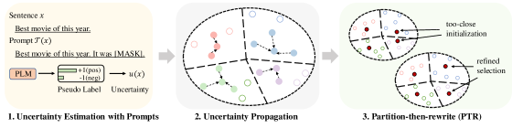
Figure 2: The illustration of the overall procedure for Patron.

In this section, we present our method, Patron, that exploits prompts for cold-start data selection. We first introduce how to leverage prompts for uncertainty estimation under cold-start scenarios. With the estimated uncertainty, we then propose two key designs, namely uncertainty propagation and partition-then-rewrite (Ptr) strategy to balance informativeness and diversity for sample selection.

4.1 Uncertainty Estimation with Prompts

We first describe how to estimate the uncertainty for unlabeled data to facilitate Patron. Given the pre-trained language model (PLM) $\mathcal{M}$ without labeled data, we leverage prompts to generate pseudo labels for uncertainty estimation. According to Eq. 1, we are able to obtain the occurring probability for different label words on each sample $x$, based on the prediction of the [MASK] token.

However, directly adopting this probability can be problematic as PLMs suffer from the mis-calibration issue Zhao et al. (2021); Hu et al. (2022), i.e., label words may have varying occurring frequencies, making some of them less likely to be predicted than the others. Thus, the prediction in Eq. 1 and the estimated uncertainty can be biased.

Being aware of this, we adopt the method in Hu et al. (2022) to calculate the contextualized prior of the label words. We first construct a support set ${\mathcal{S}}$ by choosing $k$ samples with highest $p(y_{i}|x)$ for each class $i$ as

$${\mathcal{S}}=\bigcup\limits_{i\in\{1,2,\ldots,c\}}\underset{x\in\mathcal{D}_{u}}{\operatorname{Top-k}}\ p(y_{i}|x).$$ (2)

Then, the contextualized prior is approximated by

$$P(v)\approx\frac{1}{|{{\mathcal{S}}}|}\sum_{x\in{{\mathcal{S}}}}P_{\mathcal{M}}\left(\texttt{[MASK]}=v\mid x\right),$$ (3)

which is used to calibrate the pseudo labels as

$$\widehat{y_{i}}=\left({\frac{p(y_{i}|x)}{P(\mathcal{V}(y_{i}))}}\right)/\left({\sum_{j=1}^{C}\frac{p(y_{j}|x)}{P(\mathcal{V}(y_{j}))}}\right).$$ (4)

After obtaining the pseudo labels, we use entropy Lewis and Gale (1994) as the measurement of uncertainty for each sample $x$ as

$$u(x)=-\sum_{i=1}^{C}\widehat{y_{i}}\log{\widehat{y_{i}}}.$$ (5)

4.2 Uncertainty Propagation for Data Utility Estimation

Although we have mitigated the bias for the prompt-based pseudo labels, such pseudo labels can still be inaccurate due to insufficient supervision under zero-shot settings. Under this circumstance, directly using the uncertainty in Eq. 5 for sample selection yields suboptimal results as it can be sensitive to outliers, which naturally have large model uncertainty but are less beneficial for model learning Karamcheti et al. (2021).

To remedy this issue, we leverage the kernel similarity in the embedding space to measure the correlation between data points and propagate the model uncertainty: for each data point $x$, we first calculate its embedding using SimCSE Gao et al. (2021b) as $\mathbf{z}=g(x;\theta)$, and calculate $K$-nearest neighbors based on its Euclidean distance as $\mathcal{X}_{\text{KNN}}(x)=\text{KNN}(x,\mathcal{D}_{u})$. Then, we choose the radial basis function (RBF) Scholkopf et al. (1997) as the similarity metric for two data points $x_{i}$ and $x_{j}$, denoted as

$$\kappa\left(x_{i},x_{j}\right)=\exp\left(-\rho\left\|\mathbf{z}_{i}-\mathbf{z}_{j}\right\|_{2}^{2}\right),$$ (6)

where $\mathbf{z}_{i}$ is the embedding of $x_{i}$ from the SimCSE, and $\rho$ is a hyper-parameter controlling the weight of propagation. Formally, the propagated uncertainty for $x$ can be represented as

$$\widehat{u}_{\text{prop}}(x)=u(x)+\frac{\sum_{x_{i}\in\mathcal{X}_{\text{KNN}}(x)}\kappa(x,x_{i})\cdot u(x_{i})}{|\mathcal{X}_{\text{KNN}}(x)|}.$$ (7)

We highlight that only when the sample has higher uncertainty for both itself and its neighbors will result in higher propagated uncertainty, indicating the PLMs are uncertain about the surrounding regions around the sample. In this case, actively annotating such samples will be most beneficial for PLMs.

4.3 Partition-then-rewrite (Ptr) for Diversity-Promoting Data Selection

Instead of querying one sample at a time, modern AL methods usually query a batch of samples to improve the query efficiency. In this case, querying samples without considering their correlations will lead to a redundant query set with limited performance gain Ein-Dor et al. (2020). We now present our Ptr strategy for diversity-promoting sample selection underpinned by the estimated uncertainty.

Initialization of Selection with Partition. As previous studies Aharoni and Goldberg (2020) revealed that PLMs implicitly learn sentence representations clustered by topics even without fine-tuning, we first employ K-Means clustering to partition the unlabeled pool $\mathcal{D}_{u}$ into different clusters based on their embeddings and enforce the coverage over different topics of selected samples. We follow existing works Chang et al. (2021); Hacohen et al. (2022) to set the number of clusters equal to $b$, denoted as $\mathcal{C}_{i}$ ($1\leq i\leq b$). We then use a greedy method to select one sample $q_{i}$ from $\mathcal{C}_{i}$ to initialize the selected data pool $\mathcal{Q}$ as

$$q_{i}=\mathop{\mathrm{argmax}}_{x_{j}\in\mathcal{C}_{i}}\left(\widehat{u}_{\text{prop}}(x_{j})-\beta\left\|\mathbf{z}_{j}-\mathbf{\bar{z}}_{i}\right\|_{2}^{2}\right),$$ (8)

where $\mathbf{\bar{z}}_{i}=\frac{1}{|\mathcal{C}_{i}|}{\sum_{x_{j}\in\mathcal{C}_{i}}\mathbf{z}_{j}}$ is the centroid for the cluster $i$ and $\beta$ is a hyperparameter. In this way, we aim to select data points with higher propagated uncertainty while not being faraway with most of the data points to balance between the uncertainty and diversity.

Sample Refinement with Rewriting. Although the previous steps attempt to select the most informative samples within each cluster, they fail to model the relations among samples in different clusters. As a result, samples can still be very close to other selected samples in adjacent clusters, leading to the limited overall diversity. To tackle this issue, we build an additional KNN graph to retrieve the nearest query samples from other clusters as

$$\mathcal{X}_{\text{c-KNN},i}=\text{KNN}(q_{i},\mathcal{Q}).$$ (9)

Note that we use c-KNN to denote the cluster-level KNN to differentiate from the sample-level KNN in section 4.2. To update the selected pool $\mathcal{Q}$, for cluster $i$, we add an additional regularization term to Eq. 8 to prevent samples in adjacency clusters from being overly close:

$$\widetilde{q}_{i}= \mathop{\mathrm{argmax}}_{x_{j}\in\mathcal{C}_{i}}\ (\widehat{u}_{\text{prop}}(x_{j})-\beta\left\|\mathbf{z}_{j}-\mathbf{\bar{z}}_{i}\right\|_{2}^{2}$$ (10)

$$-\gamma\sum_{q_{k}\in\mathcal{X}_{\text{c-knn},i}}\left[m-\left\|\mathbf{z}_{j}-\mathbf{z}_{k}\right\|_{2}^{2}\right]_{+}),$$

where $\gamma$ is the weight for the penalty term, $m=0.5$ is the pre-defined margin, $[\cdot]_{+}=\max(\cdot,0)$ is the gating function. To interpret the regularization term, we argue that when the distance between the selected samples in adjacency clusters is smaller than $m$, the regularization will be greater than 0 to discourage them from being selected together.

We run the above rewriting steps several times until convergence to obtain the final set $\mathcal{Q}=\{\widetilde{q}_{i}\}_{i=1}^{b}$, which usually takes 2-3 iterations. The overall procedure of Patron is in Algorithm 1.

Input: Unlabeled samples $\mathcal{X}_{u}$; Pre-trained LM $\mathcal{M}=f(\cdot;\theta)$, number of acquired samples $B$, the number of iterations $T$ ($T$=2 in this work).

// Step 1: Uncertainty Propagation for Utility Estimation.

1a. Calculate uncertainty for samples $x\in\mathcal{X}_{u}$ with prompts based on Eq. (5).

1b. Estimate uncertainty $\widehat{u}_{\text{prop}}$ with Eq. (6) and (7).

// Step 2: Predict-then-propagate (Ptr) for Diversity Promoting Selection.

2a. Run K-Means on $\mathcal{X}_{u}$ with $k$=$B$ until convergence.

2b. Select initial sample set $\mathcal{Q}^{(0)}$ based on Eq. (8).

for $t=1,2,\cdots,T$ do

       2c. Building the additional KNN graph to obtain $\mathcal{X}_{\text{c-KNN}}$ with Eq. (9).

       2d. Update $\mathcal{Q}^{(t)}$ by optimizing the selected sample within each cluster $\widetilde{q}$ with Eq. (10).

      

Output: The final selected labeled data $\mathcal{Q}^{(T)}$.

Algorithm 1 Procedures of the data selection strategy Patron.

5 Experiments

5.1 Experiment Setup

Datasets. Following prior works Yuan et al. (2020); Schröder et al. (2022), we use six text classification tasks in our experiments: IMDB Maas et al. (2011), Yelp-full Meng et al. (2019), AG News Zhang et al. (2015), Yahoo! Answers Zhang et al. (2015), DBPedia Lehmann et al. (2015), and TREC Li and Roth (2002). All the datasets are in English, and their detailed statistics are shown in Table 1. Besides, we use 3 additional datasets to evaluate the out-of-distribution (OOD) performance, the details are shown in Appendix A.3. The template and verbalizer for prompts are shown in table 7.

Evaluation Setup. Following Chang et al. (2021); Chen et al. (2021), we focus on one-round data selection in our main experiments because it can more faithfully reflect the performance of different strategies. We choose the labeling budget $|B|$ from {32, 64, 128} to simulate the few-shot scenario and align with existing works Müller et al. (2022); Shnarch et al. (2022). We also apply Patron for standard multi-round AL (see Section 5.3).

Dataset Label Type #Class $c$ #Unlabeled $|\mathcal{D}_{u}|$ #Test IMDB Sentiment 2 25k 25k Yelp-full Sentiment 5 40k 10k AG News News Topic 4 120k 7.6k Yahoo! Ans. QA Topic 10 300k 60k DBPedia Wikipedia Topic 14 420k 70k TREC Question 6 5.4k 0.5k

Table 1: Dataset Statistics. For DBPedia and Yahoo! Answers, we randomly sample 30k sample from each class due to the limited computational resource.

IMDB Yelp-full AG News Yahoo! DBPedia TREC Mean 94.1 66.4 94.0 77.6 99.3 97.2 88.1

Table 2: Fully supervised performance on six datasets.

Task	$c$	$|B|$	Random	Uncertainty	CAL	BERT-KM	Coreset	Margin-KM	ALPS	TPC	Patron (Ours)
IMDB	2	32	80.2 $\pm$ 2.5	81.9 $\pm$ 2.7	77.8 $\pm$ 2.4	79.2 $\pm$ 1.6	74.5 $\pm$ 2.9	76.7 $\pm$ 3.5	82.2 $\pm$ 3.0	82.8 $\pm$ 2.2	85.5 $\pm$ 1.5∗∗
		64	82.6 $\pm$ 1.4	84.7 $\pm$ 1.5	81.2 $\pm$ 3.4	84.9 $\pm$ 1.5	82.8 $\pm$ 2.5	84.0 $\pm$ 2.0	86.1 $\pm$ 0.9	84.0 $\pm$ 0.9	87.3 $\pm$ 1.0∗∗
		128	86.6 $\pm$ 1.7	87.1 $\pm$ 0.7	87.9 $\pm$ 0.9	88.5 $\pm$ 1.6	87.8 $\pm$ 0.8	88.2 $\pm$ 1.0	87.5 $\pm$ 0.8	88.1 $\pm$ 1.4	89.6 $\pm$ 0.4 ∗
Yelp-F	5	32	30.2 $\pm$ 4.5	32.7 $\pm$ 1.0	36.6 $\pm$ 1.6	35.2 $\pm$ 1.0	32.9 $\pm$ 2.8	32.7 $\pm$ 0.4	36.8 $\pm$ 1.8	32.6 $\pm$ 1.5	35.9 $\pm$ 1.6
		64	42.5 $\pm$ 1.7	36.8 $\pm$ 2.1	41.2 $\pm$ 0.2	39.3 $\pm$ 1.0	39.9 $\pm$ 3.4	39.8 $\pm$ 1.2	40.3 $\pm$ 2.6	39.7 $\pm$ 1.8	44.4 $\pm$ 1.1 ∗
		128	47.7 $\pm$ 2.1	41.3 $\pm$ 1.9	45.7 $\pm$ 1.3	46.4 $\pm$ 1.3	49.4 $\pm$ 1.6	47.1 $\pm$ 1.2	45.1 $\pm$ 1.0	46.8 $\pm$ 1.6	51.2 $\pm$ 0.8∗∗
AG News	4	32	73.7 $\pm$ 4.6	73.7 $\pm$ 3.0	69.4 $\pm$ 4.5	79.1 $\pm$ 2.7	78.6 $\pm$ 1.6	75.1 $\pm$ 1.8	78.4 $\pm$ 2.3	80.7 $\pm$ 1.8	83.2 $\pm$ 0.9∗∗
		64	80.0 $\pm$ 2.5	80.0 $\pm$ 2.2	78.5 $\pm$ 3.7	82.4 $\pm$ 2.0	82.0 $\pm$ 1.5	81.1 $\pm$ 2.2	82.6 $\pm$ 2.5	83.0 $\pm$ 2.4	85.3 $\pm$ 0.7∗∗
		128	84.5 $\pm$ 1.7	82.5 $\pm$ 0.8	81.3 $\pm$ 0.9	85.6 $\pm$ 0.8	85.2 $\pm$ 0.6	85.7 $\pm$ 0.3	84.3 $\pm$ 1.7	85.7 $\pm$ 0.3	87.0 $\pm$ 0.6∗∗
Yahoo! Ans.	10	32	43.5 $\pm$ 4.0	23.0 $\pm$ 1.6	26.6 $\pm$ 2.5	46.8 $\pm$ 2.1	22.0 $\pm$ 2.3	34.0 $\pm$ 2.5	47.7 $\pm$ 2.3	36.9 $\pm$ 1.8	56.8 $\pm$ 1.0∗∗
		64	53.1 $\pm$ 3.1	37.6 $\pm$ 2.0	30.0 $\pm$ 1.7	52.9 $\pm$ 1.6	45.7 $\pm$ 3.7	44.4 $\pm$ 2.8	55.3 $\pm$ 1.8	54.0 $\pm$ 1.6	61.9 $\pm$ 0.7∗∗
		128	60.2 $\pm$ 1.5	41.8 $\pm$ 1.9	41.1 $\pm$ 0.9	61.3 $\pm$ 1.0	56.9 $\pm$ 2.5	52.1 $\pm$ 1.2	60.8 $\pm$ 1.9	58.2 $\pm$ 1.5	65.1 $\pm$ 0.6∗∗
DBPedia	14	32	67.1 $\pm$ 3.2	18.9 $\pm$ 2.4	14.6 $\pm$ 1.5	83.3 $\pm$ 1.0	64.0 $\pm$ 2.8	55.1 $\pm$ 2.2	77.5 $\pm$ 4.0	78.2 $\pm$ 1.8	85.3 $\pm$ 0.9∗∗
		64	86.2 $\pm$ 2.4	37.5 $\pm$ 3.0	20.7 $\pm$ 2.0	92.7 $\pm$ 0.9	85.2 $\pm$ 0.8	78.0 $\pm$ 4.1	89.7 $\pm$ 1.1	88.5 $\pm$ 0.7	93.6 $\pm$ 0.4∗∗
		128	95.0 $\pm$ 1.5	47.5 $\pm$ 2.3	26.8 $\pm$ 1.4	96.5 $\pm$ 0.5	89.4 $\pm$ 1.5	85.6 $\pm$ 1.9	95.7 $\pm$ 0.4	95.7 $\pm$ 0.6	97.0 $\pm$ 0.2 ∗
TREC	6	32	49.0 $\pm$ 3.5	46.6 $\pm$ 1.4	23.8 $\pm$ 3.0	60.3 $\pm$ 1.5	47.1 $\pm$ 3.6	49.5 $\pm$ 1.2	60.5 $\pm$ 3.7	42.0 $\pm$ 4.4	64.0 $\pm$ 1.2∗∗
		64	69.1 $\pm$ 3.4	59.8 $\pm$ 4.2	28.8 $\pm$ 3.6	77.3 $\pm$ 2.0	75.7 $\pm$ 3.0	63.0 $\pm$ 2.5	73.0 $\pm$ 2.0	72.6 $\pm$ 2.1	78.6 $\pm$ 1.6∗∗
		128	85.6 $\pm$ 2.8	75.0 $\pm$ 1.8	50.5 $\pm$ 1.9	87.7 $\pm$ 1.5	87.6 $\pm$ 3.0	80.5 $\pm$ 2.8	87.3 $\pm$ 3.6	83.0 $\pm$ 3.8	91.1 $\pm$ 0.8∗∗
Average		32	57.2	46.1	41.5	64.0	53.2	53.8	63.9	58.9	68.4 ($\uparrow$ 4.4)
		64	68.9	56.1	46.8	71.6	68.5	65.1	71.2	70.3	75.2 ($\uparrow$ 3.6)
		128	76.6	62.5	55.6	77.6	76.1	73.2	76.8	76.3	80.2 ($\uparrow$ 2.5)

Table 3: Main results of cold-start data selection on six datasets with 10 runs. Here $c$ means the number of classes and $|B|$ is the number of acquired samples. We use accuracy as the metric, and the higher value indicates better performance. Since TREC is an imbalanced dataset, we report the F1 score in Appendix G.1. Bold and underline indicate the best and second best results for each setting respectively. We use $\pm$ to indicate standard deviation and use */** to indicate statistical significant results according to student’s t-test at level 0.05/0.01. (Same as belows.)

Task	$c$	$|B|$	Random	Uncertainty	CAL	BERT-KM	Coreset	Margin-KM	ALPS	TPC	Patron (Ours)
IMDB	2	32	81.8 $\pm$ 2.5	82.4 $\pm$ 1.7	79.6 $\pm$ 1.6	81.7 $\pm$ 1.3	85.5 $\pm$ 1.1	86.0 $\pm$ 1.2	83.5 $\pm$ 2.6	84.5 $\pm$ 0.9	86.5 $\pm$ 0.9
		64	85.6 $\pm$ 1.3	86.0 $\pm$ 1.4	81.1 $\pm$ 1.9	84.2 $\pm$ 0.9	87.8 $\pm$ 0.6	87.6 $\pm$ 0.7	84.4 $\pm$ 1.6	85.8 $\pm$ 1.2	88.8 $\pm$ 0.8∗
		128	87.7 $\pm$ 0.4	88.4 $\pm$ 0.5	83.0 $\pm$ 2.0	88.5 $\pm$ 0.8	88.9 $\pm$ 0.5	89.1 $\pm$ 0.4	88.9 $\pm$ 0.3	88.0 $\pm$ 0.5	89.3 $\pm$ 0.3
Yelp-F	5	32	48.9 $\pm$ 1.3	46.6 $\pm$ 0.9	47.9 $\pm$ 0.6	45.5 $\pm$ 1.0	46.0 $\pm$ 1.5	47.5 $\pm$ 1.1	47.0 $\pm$ 1.0	49.8 $\pm$ 0.5	50.5 $\pm$ 0.8∗
		64	51.0 $\pm$ 0.8	49.9 $\pm$ 0.8	49.4 $\pm$ 1.1	51.9 $\pm$ 0.5	48.8 $\pm$ 1.2	52.6 $\pm$ 0.6	52.8 $\pm$ 0.5	52.3 $\pm$ 0.7	53.6 $\pm$ 0.3∗∗
		128	51.3 $\pm$ 0.9	50.8 $\pm$ 0.6	48.7 $\pm$ 1.6	51.5 $\pm$ 1.4	53.7 $\pm$ 1.1	54.2 $\pm$ 0.7	51.7 $\pm$ 0.5	51.0 $\pm$ 0.7	55.6 $\pm$ 0.6∗∗
AG News	4	32	83.1 $\pm$ 1.2	82.8 $\pm$ 2.0	81.4 $\pm$ 1.0	84.9 $\pm$ 0.9	85.1 $\pm$ 1.5	84.6 $\pm$ 1.7	84.2 $\pm$ 0.8	85.6 $\pm$ 1.0	86.8 $\pm$ 0.3∗∗
		64	84.5 $\pm$ 1.3	84.3 $\pm$ 1.4	82.6 $\pm$ 1.2	86.5 $\pm$ 0.8	86.4 $\pm$ 1.3	85.9 $\pm$ 0.7	86.2 $\pm$ 0.5	85.6 $\pm$ 0.5	87.4 $\pm$ 0.6∗
		128	84.9 $\pm$ 0.5	83.1 $\pm$ 0.8	83.0 $\pm$ 0.9	87.6 $\pm$ 0.4	87.5 $\pm$ 0.3	87.1 $\pm$ 0.4	87.5 $\pm$ 0.4	87.0 $\pm$ 0.6	87.8 $\pm$ 0.3
Yahoo! Ans.	10	32	58.5 $\pm$ 4.0	55.0 $\pm$ 3.0	54.0 $\pm$ 1.5	61.4 $\pm$ 1.8	55.3 $\pm$ 2.1	57.8 $\pm$ 2.6	61.9 $\pm$ 0.9	57.0 $\pm$ 1.6	63.2 $\pm$ 1.2∗
		64	62.2 $\pm$ 1.0	60.4 $\pm$ 0.7	58.6 $\pm$ 1.3	62.8 $\pm$ 0.7	59.5 $\pm$ 0.7	58.8 $\pm$ 1.2	63.3 $\pm$ 0.8	60.8 $\pm$ 0.7	66.2 $\pm$ 0.3∗∗
		128	64.7 $\pm$ 1.3	63.0 $\pm$ 1.2	60.1 $\pm$ 1.8	65.4 $\pm$ 1.2	62.7 $\pm$ 1.0	65.4 $\pm$ 0.7	65.9 $\pm$ 0.7	66.2 $\pm$ 0.6	67.6 $\pm$ 0.5∗∗
DBPedia	14	32	89.1 $\pm$ 3.0	77.9 $\pm$ 2.8	58.9 $\pm$ 1.3	94.1 $\pm$ 1.4	92.0 $\pm$ 0.6	90.6 $\pm$ 0.7	91.2 $\pm$ 2.8	94.3 $\pm$ 0.5	95.4 $\pm$ 0.4∗∗
		64	95.5 $\pm$ 1.2	86.3 $\pm$ 1.0	63.5 $\pm$ 1.7	95.8 $\pm$ 0.7	96.1 $\pm$ 0.4	95.5 $\pm$ 0.6	95.4 $\pm$ 0.7	95.6 $\pm$ 0.5	96.9 $\pm$ 0.2∗∗
		128	96.0 $\pm$ 0.6	87.8 $\pm$ 0.7	78.1 $\pm$ 2.0	97.2 $\pm$ 0.2	96.4 $\pm$ 0.5	96.6 $\pm$ 0.4	96.8 $\pm$ 0.3	97.0 $\pm$ 0.3	97.4 $\pm$ 0.1∗
TREC	6	32	69.4 $\pm$ 2.8	66.4 $\pm$ 3.5	41.6 $\pm$ 2.5	68.1 $\pm$ 2.3	61.0 $\pm$ 4.6	64.8 $\pm$ 2.7	72.1 $\pm$ 2.3	59.5 $\pm$ 3.3	76.1 $\pm$ 1.1∗∗
		64	75.4 $\pm$ 1.4	68.0 $\pm$ 2.3	49.8 $\pm$ 1.5	78.8 $\pm$ 2.0	78.6 $\pm$ 1.3	74.2 $\pm$ 1.4	80.6 $\pm$ 0.9	77.8 $\pm$ 1.5	81.9 $\pm$ 1.3∗
		128	85.0 $\pm$ 2.1	78.8 $\pm$ 2.0	67.2 $\pm$ 2.7	85.6 $\pm$ 1.8	84.2 $\pm$ 2.4	78.0 $\pm$ 1.9	86.5 $\pm$ 2.0	80.6 $\pm$ 1.4	88.9 $\pm$ 1.0∗∗
Average		32	71.9	68.6	60.4	72.6	71.0	71.9	73.2	71.8	76.5 ($\uparrow$ 3.3)
		64	75.7	72.5	64.2	76.7	69.5	75.7	77.1	76.3	79.5 ($\uparrow$ 2.4)
		128	78.2	75.3	70.0	79.3	78.9	78.4	79.5	78.3	81.1 ($\uparrow$ 1.6)

Table 4: Experimental result for prompt-based learning Gao et al. (2021a) on six datasets with 10 runs.

Baselines. We include both traditional AL baselines (Random, Uncertainty, CAL, Coreset) as well as recently-proposed cold-start AL baselines (BERT-KM, Margin-KM, ALPS, TPC).

$\diamond$ Random: It acquires annotations randomly with the annotation budget.
$\diamond$ Uncertainty Schröder et al. (2022): It acquires annotations on samples with the highest uncertainty in Eq. 5 after calibration. We use Entropy Lewis and Gale (1994) as the uncertainty estimate.
$\diamond$ CAL Margatina et al. (2021): It selects samples based on the KL divergence between the prediction of itself and that of its neighbors.
$\diamond$ Coreset Sener and Savarese (2018): It selects samples such that the largest distance between a data point and its nearest center is minimized.
$\diamond$ BERT-KM Chang et al. (2021): It first uses K-Means to cluster pre-trained embeddings and then selects one example from each cluster that is closest to the center of the cluster.
$\diamond$ Margin-KM Müller et al. (2022): It utilizes K-Means clustering to group pre-trained embeddings, followed by the selection of samples with the minimum margin between the two most likely probabilities from each cluster. Unlike Ptr, Margin-KM does not explicitly control the distance among selected samples, nor does it employ uncertainty propagation to improve data utility estimation.
$\diamond$ ALPS Yuan et al. (2020): It uses the masked language model (MLM) loss of BERT to generate surprisal embeddings to query samples.
$\diamond$ TPC Hacohen et al. (2022): It is the most recent method for CSAL, which first calculates the density for each data point, and then selects those with the highest density from each cluster.

Implementation Details. We choose RoBERTa-base Liu et al. (2019) from the Hugging Face codebase Wolf et al. (2020) as the backbone for all the compared methods. For prompt-based learning, we use OpenPrompt Ding et al. (2022) as the codebase. More details are in Appendix C.

Hyperparameters. The hyperparameters settings are given in Appendix C.4 and C.5.

5.2 Main Results

Table 3 reports the performance of Patron and the baselines under different budgets $|B|$ on 10 runs. We have the following observations:

$\diamond$ Compared with the baselines, Patron achieves the best overall performance on the six datasets, with an average gain of 3.2%-6.9% over the strongest baselines under different annotation budgets. Moreover, with 128 labels only (<0.5% of total labeled data), Patron obtains 91.0% of the fully supervised performance on the average of six datasets. It is also worth noting that Patron also lead to more stable results — it achieves lower standard deviations when compared with baselines on 14 of 18 cases. These results justify the benefits of Patron in cold-start setting.

$\diamond$ We observe the performance gains are more significant for datasets with larger number of classes (e.g. TREC, Yahoo!). This observation further strengthens the superiority of Patron in resolving label scarcity issue brought by cold-start setting, because for datasets with more classes, each class would have less labeled data given a fixed budget.

$\diamond$ Similar to the findings in Hacohen et al. (2022), pure uncertainty-based AL methods (e.g. CAL) do not perform well under cold-start settings. The reason is two-fold: (1) these methods focus on choosing ‘hard samples’ without considering the sample diversity, leading to imbalanced label distribution for acquired samples; (2) they do not consider the potential bias in uncertainty estimation.

$\diamond$ Diversity-based methods (e.g. BERT-KM, ALPS) generally achieve performance gains over the uncertainty-based strategy. Intriguingly, we find that directly using K-Means performs better than other hybrid approaches with more complicated operations (e.g. TPC, ALPS) for data selection, especially for datasets with larger number of classes. This is because these complex methods often ignore the diversity for selected samples in adjacent clusters and therefore underperform Patron.

5.3 Adapting Patron to Other Settings

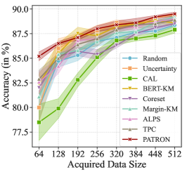
(a) AG News

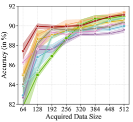
(b) IMDB

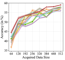
(c) Yelp-full

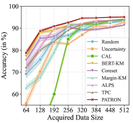
(d) TREC

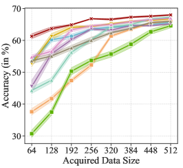
(e) Yahoo!

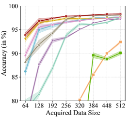
(f) DBPedia

Figure 3: The comparision of Patron with other baselines under standard multi-round AL setting.

Here, we adapt Patron to other related settings to demonstrate its general applicability.

Multi-round Low-budget Active Learning. Patron can also be applied in standard multi-round active learning. We study an AL setting where the labeling budget is set to $512$ and the queries to $64$ labels in each round ($8$ rounds in total). More details are in Appendix B.4. Figure 3 shows the result of Patron and the baselines on 4 datasets. From the results, we observe that Patron also achieves competitive performance when compared with baselines. One exception is the IMDB dataset, where uncertainty-based methods outperform Patron when the annotation size is larger than 256. This phenomenon indicates that when the labels are abundant and the cold-start issue is mitigated, uncertainty-based methods can be employed to further enhance the performance Yuan et al. (2020). In this case, we can design hybrid strategies to combine Patron and uncertainty-based methods for acquiring labeled data.

Prompt-based Few-shot Learning. Prompt-based Learning Liu et al. (2021b) is another popular approach to promote the data efficiency for PLMs. To demonstrate the compatibility of Patron with prompt-based learning, we leverage the same prompt as the pseudo label generation part (Sec.  4.2), and use the same pipeline as LM-BFF Gao et al. (2021a) to fine-tune the PLM. Table 4 shows the result of few-shot prompt-based learning using {32, 64, 128} samples. From the result, we find that LM-BFF performs better than vanilla fine-tuning with 12.5% gain on average, which makes further improvements difficult. However, Patron still outperforms the best baseline by 2.0%–4.5%. We remark that Patron is naturally suitable for prompt-based learning, as we leverage the uncertainty derived from prompt-based predictions to assist data selection.

Semi-supervised Learning. When there are large amounts of unlabeled data, Semi-supervised Learning (SSL) methods can be used to improve AL performance. Here, we choose two representative SSL methods: unsupervised data augmentation (UDA) Xie et al. (2020) and self-training (ST) Du et al. (2021); Yu et al. (2021). Table 5 exhibits the results for Patron and baselines. Notably, when the selection strategy is sub-optimal, directly adopting SSL approaches cannot bring additional performance gains. This is because the PLM fine-tuned on those samples is likely to produce incorrect pseudo labels. As a result, such incorrect labeled samples will hurt the final performance. In contrast, we observe that Patron leads to better performance for PLMs than baselines, which indicates the potentials of combining Patron with SSL approaches.

Dataset ($\rightarrow$)	AG News		TREC
Method ($\downarrow$)	UDA	ST	UDA	ST
Random	78.0 $\pm$ 2.1	82.9 $\pm$ 1.5	56.5 $\pm$ 3.0	56.0 $\pm$ 2.5
Uncertainty	74.5 $\pm$ 1.6	71.9 $\pm$ 2.0	51.6 $\pm$ 1.5	44.2 $\pm$ 2.3
CAL	71.0 $\pm$ 2.0	66.8 $\pm$ 2.7	23.5 $\pm$ 2.1	22.4 $\pm$ 2.1
BERT-KM	83.4 $\pm$ 1.0	85.2 $\pm$ 1.1	68.4 $\pm$ 1.6	67.2 $\pm$ 2.1
Coreset	82.1 $\pm$ 1.0	85.4 $\pm$ 0.6	51.1 $\pm$ 2.0	48.0 $\pm$ 2.4
Margin-KM	77.1 $\pm$ 1.2	83.1 $\pm$ 1.4	54.4 $\pm$ 1.8	50.5 $\pm$ 1.6
ALPS	82.7 $\pm$ 0.8	84.5 $\pm$ 0.8	68.8 $\pm$ 1.6	71.0 $\pm$ 1.2
TPC	83.8 $\pm$ 0.5	85.5 $\pm$ 0.4	48.0 $\pm$ 1.9	48.8 $\pm$ 2.1
Patron	84.9 $\pm$ 0.5	86.4 $\pm$ 0.3	71.7 $\pm$ 1.0	73.6 $\pm$ 0.5

Table 5: Experimental results for combining two semi-supervised learning: unsupervised data augmentation (UDA) and self-training (ST) with different data selection strategies on 2 datasets with the budget of 32 labels.

5.4 Out-of-Distribution (OOD) Evaluation

Datasets	SST-2	IMDB	IMDB	SST-2	IMDB	IMDB	SST-2	IMDB	IMDB
	Test	Contrast	Counterfactual	Test	Contrast	Counterfactual	Test	Contrast	Counterfactual
Budget $|B|$	32			64			128
Random	76.2 $\pm$ 2.4	76.1 $\pm$ 4.0	80.5 $\pm$ 4.7	80.0 $\pm$ 1.2	77.0 $\pm$ 1.1	80.8 $\pm$ 2.0	83.0 $\pm$ 2.1	83.8 $\pm$ 1.2	87.9 $\pm$ 1.6
Uncertainty	78.0 $\pm$ 2.3	66.0 $\pm$ 4.0	69.9 $\pm$ 3.1	80.0 $\pm$ 1.5	75.5 $\pm$ 0.4	82.6 $\pm$ 2.9	83.6 $\pm$ 2.3	81.6 $\pm$ 1.0	85.6 $\pm$ 0.8
CAL	76.2 $\pm$ 3.1	76.5 $\pm$ 2.9	77.6 $\pm$ 3.2	77.5 $\pm$ 3.5	76.7 $\pm$ 3.9	78.7 $\pm$ 3.8	78.3 $\pm$ 3.4	85.4 $\pm$ 0.9	90.8 $\pm$ 0.8
BERT-KM	76.9 $\pm$ 1.3	75.6 $\pm$ 2.0	81.2 $\pm$ 2.0	81.5 $\pm$ 1.4	82.3 $\pm$ 4.2	85.8 $\pm$ 4.4	84.6 $\pm$ 3.0	86.2 $\pm$ 1.4	90.3 $\pm$ 0.5
Coreset	71.6 $\pm$ 2.0	60.7 $\pm$ 3.4	63.7 $\pm$ 4.3	79.6 $\pm$ 3.4	66.3 $\pm$ 5.5	66.6 $\pm$ 4.4	82.2 $\pm$ 2.5	80.5 $\pm$ 2.6	83.7 $\pm$ 3.6
Margin-KM	71.5 $\pm$ 3.4	61.2 $\pm$ 3.0	57.5 $\pm$ 2.4	80.0 $\pm$ 3.0	74.9 $\pm$ 1.6	79.3 $\pm$ 2.5	80.9 $\pm$ 3.5	86.8 $\pm$ 2.0	90.1 $\pm$ 2.3
ALPS	78.5 $\pm$ 1.9	78.5 $\pm$ 2.7	81.8 $\pm$ 2.4	77.8 $\pm$ 2.8	83.1 $\pm$ 1.8	87.5 $\pm$ 1.5	83.0 $\pm$ 3.2	84.4 $\pm$ 1.5	89.1 $\pm$ 1.4
TPC	77.8 $\pm$ 3.8	72.1 $\pm$ 5.0	76.9 $\pm$ 6.1	81.0 $\pm$ 0.9	74.2 $\pm$ 1.2	77.1 $\pm$ 2.2	79.3 $\pm$ 3.1	83.0 $\pm$ 2.2	87.5 $\pm$ 2.6
Patron	81.3 $\pm$ 2.6	81.9 $\pm$ 2.3	85.3 $\pm$ 2.1	80.8 $\pm$ 2.7	84.7 $\pm$ 1.8	88.9 $\pm$ 1.0	85.9 $\pm$ 2.0	87.0 $\pm$ 1.5	92.2 $\pm$ 1.3

Table 6: Full results of the evaluation on OOD tasks for IMDB datasets.

We conduct Out-of-Distribution (OOD) evaluation to verify whether the methods can robustly select representative samples for the task instead of overfitting one specific dataset. We use IMDB dataset as a source domain for data selection and fine-tuning, and then directly evaluate the fine-tuned model on 3 out-of-domain datasets (see Appendix A.3 for details): SST-2 Socher et al. (2013), IMDB Contrast Set (IMDB-CS) Gardner et al. (2020), and IMDB Counterfactually Augmented Dataset (IMDB-CAD) Kaushik et al. (2020).

As shown in Table 6, diversity-based approaches also perform better than uncertainty-based methods on OOD tasks, due to the better coverage of the selected samples. However, Patron still outperforms these baselines by 3.2% on average. The performance gains illustrate that Patron can discover informative samples to truly enable the PLM to capture task-specific linguistic knowledge instead of spurious features and improve the PLM’s generalization ability under limited budget.

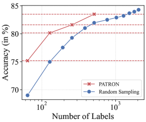
Figure 4: The comparison of Patron and random sampling with various volume of labeled data.

5.5 Label Efficiency Analysis

Fig. 4 demonstrate the average performance on six datasets with different volume of labeled data selected via random sampling and Patron. The label efficiency curve for each dataset is shown in Fig. 7. We notice that Patron largely alleviates the label scarsity bottleneck: with 128 labels as the budget, Patron achieves better performance with 2X labels. Furthermore, after collecting 512 labels with multi-round AL (Sec 5.3), Patron achieves 95% of the fully-supervised performance on average, which is comparable with the performance using 3X labels based on random sampling. These results clearly justify that Patron is capable of promoting the label efficiency of PLMs.

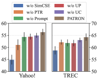
(a) Ablation Study

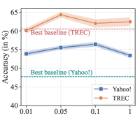
(b) Effect of $\rho$.

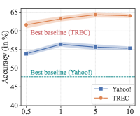
(c) Effect of $\beta$.

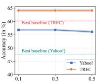
(d) Effect of $\gamma$.

Figure 5: Ablation and Hyper-parameter Study.

5.6 Ablation Study

We study the effects of different components of Patron, including the prompt-based uncertainty calibration in Eq. 4 and propagation in Eq. 7 (Prompt, UC and UP respectively), the feature encoder (SimCSE), as well as the Ptr strategy. We evaluated on the TREC and Yahoo! datasets with 32 labels as the budget. The results in Fig. 5(a) show that all these components contribute to the final performance of Patron. We find that the usage of SimCSE brings considerable performance gains, as the embeddings generated via RoBERTa-base suffer from the degeneration issue Li et al. (2020) and become less discriminative. Besides, the usage of prompts, as well as the two dedicated designs, namely uncertainty calibration and propagation enable us to complement the SimCSE embeddings with the prompt-based pseudo labels and improve the performance significantly. Lastly, Ptr helps regularize the distance among selected samples, which is also beneficial for AL.

5.7 Patron is Robust to Hyperparameters

Patron introduces three additional hyperparameters, namely $\rho$ in Eq. 6, $\beta$ in Eq. 8 and $\gamma$ in Eq. 10. To investigate their effects on the final performance, Figure  5(b)–5(d) show the effects of them in Patron on two datasets with 32 labels as the budget. The results on other datasets are deferred to Figure 6 in Appendix G.2.

In general, the model is robust to them as the Patron outperforms the baselines in most cases with different sets of hyperparameters. We also notice that the performance is not sensitive to $\gamma$. Besides, the performance first increases then decreases for both $\rho$ and $\beta$. For $\rho$, setting it too large makes the propagated uncertainty too small, and setting it too small makes the influence of neighbor samples too strong and hurt data utility estimation. For $\beta$, the sampled data is less informative with a too large $\beta$, while being too close from others during initialization with a too small $\beta$. In practice, we can always search for optimal hyperparameters in an iterative manner: in each iteration, we only tune one hyperparameter and keep others fixed. In addition, there are automatically hyperparameter optimization tools Akiba et al. (2019) that can efficiently find the optimal hyperparameters.

To sum up, although Patron includes additional hyperparameters, it will not introduce much difficulty for hyperparameter tuning. Instead, these hyperparameters improve the modeling flexibility of Patron to adapt to different tasks.

6 Discussion

Connection to Weakly-supervised Learning. Our method can also be considered as weakly-supervised data selection, where only class-indicating keywords as well templates are provided. Although such formulations have been adopted for NLP tasks Meng et al. (2019, 2020); Hu et al. (2022) (see Zhang et al. (2022a) for a detailed survey), how to effectively leverage such weak supervision signals for data selection has not been widely explored in NLP. In this study, we tackle this research problem to facilitate few-shot PLM fine-tuning, and demonstrate such task-specific weak supervision is beneficial for downstream tasks.

Data Selection under Low and High Budget. In this study, we mainly focus on cold-start setting to select data without any labeled data. This is different from traditional AL pipelines, and we do not claim Patron outperforms AL methods under high-budget scenarios. However, experiments show our method shines under low-budget setting, and Patron can also be leveraged in earlier rounds of standard AL to improve the label efficiency.

7 Conclusion

We develop Patron, a prompt-based data selection method for pre-trained language models (PLMs) under cold-start scenarios. By leveraging prompts, we can distill the task-specific knowledge from the frozen PLM to guide data acquisition. Moreover, we develop two techniques, namely uncertainty propagation and predict-then-rewrite (Ptr) to achieve both sample representativeness and diversity. The experiments on six text classification tasks demonstrate the superiority of Patron against baselines for few-shot PLM fine-tuning.

Limitations

In this work, we focus on designing strategies for PLMs with the MLM-style pre-training objective and do not account for other types of pre-trained language models such as discriminative PLMs Clark et al. (2020); Shen et al. (2021). However, as there are recent works that aim to design prompts for discriminative PLMs Yao et al. (2022); Xia et al. (2022), Patron can be potentially combined with them to improve the data efficiency.

We are also aware that there exists advanced few-shot fine-tuning techniques for PLMs recently (Hu et al., 2022; Tam et al., 2021; Zhang et al., 2022b, inter alia). We argue that Patron does not rely on a specific fine-tuning method, and can be combined with them to further improve the performance.

Dataset	Domain	Classes $c$	$\#$Unlabeled	#Test	Type	Template	Label words
IMDB	Movie Review	2	25k	25k	sentiment	$\langle S\rangle$. It was [MASK].	terrible, great
Yelp-full	Restaurant Review	2	560k	38k	sentiment	$\langle S\rangle$. It was [MASK].	terrible, bad, okay, good, great
AG News	News	4	120k	7.6k	News Topic	[MASK] News: $\langle S\rangle$	World, Sports, Business, Tech
Yahoo! Answers	Web QA	10	300k	60k	QA Topic	[Category: [MASK]] $\langle S\rangle$	Society, Science, Health, Education, Computer,
							Sports, Business, Entertainment, Relationship, Politics
DBPedia	Wikipedia Text	14	420k	70k	Wikipedia Topic	$\langle T\rangle\langle S\rangle.\langle T\rangle$ is a [MASK]]	Company, School, Artist, Athlete, Politics,
							Transportation, Building, Mountain, Village,
							Animal, Plant, Album, Film, Book
TREC	Web Text	6	5k	0.6k	Question Topic	$\langle S\rangle$. It was [MASK].	Expression, Entity, Description, Human, Location, Number

Table 7: Statistics, manual templates, and label words used in our experiments. $c$: number of classes.

Appendix A Datasets Details

A.1 Datasets for the Main Experiment

The seven benchmarks in our experiments are all publicly available. Below are the links to downloadable versions of these datasets.

$\diamond$ IMDB: We use the datasets from https://huggingface.co/datasets/imdb.

$\diamond$ Yelp-full: Dataset is available at https://github.com/yumeng5/WeSHClass/tree/master/yelp.

$\diamond$ AG News: Dataset is available at https://huggingface.co/datasets/ag_news.

$\diamond$ Yahoo! Answers: Dataset is available at https://huggingface.co/datasets/yahoo_answers_topics.

$\diamond$ DBPedia: Dataset is available at https://huggingface.co/datasets/dbpedia_14.

$\diamond$ TREC: Dataset is available at https://huggingface.co/datasets/trec. Note that we only use the coarse-grained class labels.

A.2 Train/Test Split

For all the datasets, we use the original train/test split from the web. To keep the size of the development set small Bragg et al. (2021), we randomly sample 32 data from the original training set as the development set, and regard the remaining as the unlabeled set $\mathcal{D}_{u}$.

Datasets	Zero-shot Acc.	Zero-shot Acc.	NMI	ARI
	(in %)	after UC. (in %)
IMDB	73.29	83.13	0.249	0.319
Yelp-full	32.76	38.62	0.079	0.056
AG News	81.43	80.66	0.443	0.432
Yahoo! Answers	44.13	47.55	0.274	0.193
DBPedia	73.78	81.13	0.717	0.595
TREC	35.69	38.51	0.111	0.088

Table 8: Quality of Prompts and SimCSE embeddings for six datasets used in our experiments.

A.3 Datasets for OOD Evaluation

We use 3 datasets as OOD tasks for evaluating Patron and baselines. The details are listed as belows.

$\diamond$ SST-2 Socher et al. (2013) is another movie review sentiment analysis dataset. The key difference between the SST-2 and IMDB datasets is that they consist of movie reviews with different lengths. We use the original validation set (containing 872 samples) for evaluation.

$\diamond$ IMDB Contrast Set (IMDB-CS) Gardner et al. (2020) and IMDB Counterfactually Augmented Dataset (IMDB-CAD) Kaushik et al. (2020) are two challenging sentiment analysis datasets (both of them contain 488 examples) which can be used to evaluate a model’s true linguistic capabilities more accurately. Specifically, for IMDB-CS, NLP researchers creates contrast sets via manually change the ground-truth label of the test instances in a small but semantically meaningful way. For IMDB-CAD, annotators are required to make minor changes to examples in the original IMDB dataset to flip the sentiment labels, without changing the majority of contents.

A.4 Prompt Format

For these datasets, we directly use manual prompts that have been used in previous works Schick and Schütze (2021a); Gao et al. (2021a); Hu et al. (2022). The details of the prompts used in our experiments is listed in Table 7.

A.5 The Quality of Prompts and SimCSE Embeddings

We list the quality of prompts as well as SimCSE embeddings in this part. From prompts, we use the zero-shot accuracy for the unlabeled data as the quality measure. From embeddings, we perform clustering to evaluate the quality of the SimCSE embeddings. We use K-Means as the clustering method, and use two metrics, namely Normalized Mutual Information (NMI), and Adjusted Rand Index (ARI) Vinh et al. (2010) for evaluation. For these metrics, higher value indicates better quality. The results are shown in Table 8. We observe that although the quality of these two terms are high for some tasks such as IMDB and AG News, for other tasks, the embeddings are less discriminative and the prompts are less accurate. These pose specific challenges for Patron to select most useful data with noisy prompt-based predictions with the imperfect embeddings.

Appendix B Experiment Setups

B.1 Main Experiment Setups

In experiments, both our method and baselines are run with 5 different random seed and the result is based on the average performance on them. We have show both the mean and the standard deviation of the performance in our experiment sections.

B.2 Experiment Setups for Prompt-based Few-shot Learning

We mainly use the pipeline in LM-BFF Gao et al. (2021a) for prompt-based learning. For both Patron and baselines, we use the prompt defined in Table 7 to fine-tune PLMs. We use OpenPrompt toolkit Ding et al. (2022) for implementation and use RoBERTa-base as the backbone for prompt-based learning.

B.3 Experiment Setups for Semi-supervised Learning

For semi-supervised learning, we mainly adopt Unsupervised Data Augmentation (UDA) Xie et al. (2020) and self-training Du et al. (2021) as two examples. The main idea of UDA is leveraging data augmentation techniques (TF-IDF word replacement or back translation) with the consistency-based loss for unlabeled data to improve the model performance. Since we do not have access to TPU service and need to use smaller amount of unlabeled data, we implement UDA on our own. For self-training, it generates pseudo labels on unlabeled data, and encourages models to output confident predictions on these data. Please refer to the original papers for the details of these methods.

B.4 Experiment Setups for Standard Multi-round Active Learning

For standard multi-round active learning, we follow the standard multi-round active learning pipelines introduced in Margatina et al. (2021); Yuan et al. (2020), but in the beginning round, no initial labeled data is given. In each round, we train the PLM from scratch to avoid overfitting to the data collected in earlier rounds as observed by Hu et al. (2019).

Appendix C Details on Implementations

C.1 Computational Setups

Overall we report the results of 3240 BERT fine-tuning runs for main experiments (2 settings × 6 datasets × 3 labeling budgets × 9 methods × 10 repetitions). The computing infrastructure used for experiments are listed as follows.
System: Ubuntu 18.04.3 LTS; Python 3.8; Pytorch 1.10.
CPU: Intel(R) Core(TM) i7-5930K CPU @ 3.50GHz.
GPU: NVIDIA A5000.

Hyper-parameter	IMDB	Yelp-full	AG News	Yahoo!	DBPedia	TREC
Maximum Tokens	256	256	128	128	128	64
Learning Rate	2e-5	2e-5	5e-5	5e-5	1e-5	2e-5
$k$	1000					50
$\rho$	0.05	0.1	0.1	0.1	0.1	0.1
$\gamma$	0.3	0.3	0.5	0.3	0.1	0.3
$\beta$	0.5	5	0.5	1	5	5
$m$	0.5

Table 9: Hyper-parameter configurations. Note that we only keep certain number of tokens.

C.2 Number of Parameters

In our main experiments, Patron and all baselines use RoBERTa-base Liu et al. (2019) with a task-specific classification head on the top as the backbone, which contains 125M trainable parameters. We do not introduce any other parameters in our experiments.

C.3 Implementations of Baselines

For Random, Uncertainty, BERT-KM, Margin-KM, we implement them by ourselves. For other baselines, we run the experiments based on the implementations on the web. We list the link for the implementations as belows:

$\diamond$ Coreset: https://github.com/google/active-learning/tree/master/sampling_methods.

$\diamond$ ALPS: https://github.com/forest-snow/alps.

$\diamond$ CAL: https://github.com/mourga/contrastive-active-learning.

$\diamond$ TPC: https://github.com/avihu111/TypiClust.

C.4 Hyper-parameters for Model Training

We use AdamW Loshchilov and Hutter (2019) as the optimizer, and choose the learning rate from $\{1\times 10^{-5},2\times 10^{-5},5\times 10^{-5}\}$, the batch size from $\{4,8,16\}$, and set the number of training epochs to $15$ for both fine-tuning, prompt-based few-shot learning, and multi-round active learning.

For semi-supervised learning, we initialize the model with the RoBERTa-base fine-tuned on the acquired labeled data (based on different data selection strategies). Then, we set the batch size for unlabeled data to $32$, and choose the learning rate from $\{1\times 10^{-6},5\times 10^{-6},1\times 10^{-5}\}$ since we empirically find that smaller learning rates lead to the better training stability. We use the model with best performance on the development set to determine the best set of parameter for testing.

C.5 Hyper-parameters for AL Implementation

Patron introduces several hyper-parameters including $k$ in Eq. 2, $K$ for calculating $\mathcal{X}_{\text{KNN}}(x)$ ,$K^{\prime}$ for calculating $\mathcal{X}_{\text{c-KNN}}(x)$, $\beta,\gamma,m$ in Eq. 8, $\rho$ in Eq. 6, but most of them are keep fixed during our experiments, thus it does not require heavy hyper-parameter tuning.

In our experiments, we keep $K^{\prime}=10$, $K=50$, $m=0.5$ for all datasets. For other parameters, we use a grid search to find the optimal setting for each datasets. We search $\rho$ from $\{0.01,0.05,0.1,1\}$, $\beta$ from $\{0.5,1,5,10\}$, $\gamma$ from $\{0.1,0.3,0.5\}$. All results are reported as the average over ten runs. The number for hyper-parameters we use are shown in Table 9.

For other baselines, we follow the exact parameter tuning method mentioned in the original paper for hyperparameter tuning. For CAL Margatina et al. (2021) and TPC Hacohen et al. (2022), we tune the number for KNN $k$ from $[5,10,20,50]$ and report the best performance.

Appendix D Adapting Patron to Multi-round AL

When applying Patron to Multi-round AL, since there exists a warm-start model with a set of labeled data, we directly use the embedding from the warm-start model to generate features and leverage it for uncertainty estimation. After that, uncertainty propagation can be directly adopted for estimating the utility of training data. For the Ptr step, since we already have a smaller number of the labeled samples $\mathcal{D}_{l}$, the Eq. 9 can be refined as

$$\mathcal{X}_{\text{c-KNN},i}=\text{KNN}(q_{i},\mathcal{Q}\cup\mathcal{D}_{l}),$$ (11)

as we don’t want the selected samples to be too close to samples in $\mathcal{D}_{l}$. The other steps of Ptr are remain unchanged.

Appendix E Time Complexity of Patron

Method Time Random 0.1s Uncertainty 461s CAL 649s BERT-KM 724s Coreset 872s Margin-KM 1389s ALPS 682s TPC 1448s Patron 1480s

Table 10: The running time of Patron and different baselines on Yahoo! Answers dataset.

The additional time introduced by Patron mainly comes from the KNN step in the uncertainty propagation as well as the K-Means partitioning. However, these operations have been efficiently supported via approximate nearest neighbor search (ANN) Johnson et al. (2019). As a result, Patron will not incur excessive computational overhead.

Table 10 exhibits the running time of Patron and baselines on the Yahoo! Answers dataset for selecting 64 samples. Overall, compared with the recent baselines such as TPC Hacohen et al. (2022) and Margin-KM Müller et al. (2022), the additional time introduced is small. In particular, the uncertainty propagation takes 114 seconds, and the predict-then-propagate step only takes 5 seconds. This verifies that our key designs do not takes much time and are scalable for large datasets.

Appendix F Additional Analysis

In this section, we provide detailed comparison on different data selection strategies, aiming to better understand their relative advantages and disadvantages. Specifically, we follow the method in Ein-Dor et al. (2020) and focus on three types of metrics: class distribution, feature diversity, and representativeness. All of these metrics are calculated based on the results with 128 labels as the budget.

F.1 Class Distribution of the Selected Data

We calculate the class distribution of the selected samples. Denote the number of samples selected from each class as $n_{1},\ldots,n_{c}$ where $\sum_{i=1}^{c}n_{i}=|B|$ ($|B|=128$ in this case), we use two metrics, namely imbalance value and label distribution divergence value to measure the class distribution. Specifically, imbalance value (IMB) is calculated as

$$\operatorname{IMB}=\frac{\max_{i=1,\ldots,c}(n_{i})}{\min_{i=1,\ldots,c}(n_{i})}.$$ (12)

The higher IMB value indicates the more imbalanced distribution. Note that when data from one or more classes are totally not sampled, the IMB value will become infinity (+inf).

As the label distribution of some datasets are imbalanced, we introduce another metrics named label distribution divergence, to calculate the distance between the distribution of ground-truth labels and labels sampled by baselines or our method. Specifically, denote $p_{i}$ as the frequency of label $i$. Then the label distribution divergence (LDD) is calculated as

$$\operatorname{LDD}=\mathcal{D}_{\operatorname{KL}}\left(q||p\right)=-\sum_{i}q_{i}\log{(p_{i}/q_{i})}.$$ (13)

where $q_{i}=n_{i}/|B|$ is equal to the frequency of class $i$ in the selected samples. The higher LDD value indicates the more biased sampled distribution from the original distribution.

Table 11 and 12 show the IMB and LDD value for all methods on six datasets. From the results, we find that for uncertainty-based approaches, the corresponding values for these two metrics are very high. This indicates that the selected samples are highly imbalanced. As there does not exist any startup labels for cold-start data selection, fine-tuning PLMs on such imbalanced data leads to the biased predictions. These results explain why the performance of such uncertainty-based methods are extremely poor under cold-start scenarios.

Task	$c$	Random	Uncertainty	CAL	BERT-KM	Coreset	Margin-KM	ALPS	TPC	Patron
IMDB	2	1.207	6.111	7.000	1.286	1.000	1.133	1.783	2.765	1.286
Yelp-F	5	1.778	3.800	13.500	2.000	6.000	1.600	2.833	5.200	2.250
AG News	4	1.462	28.000	2.000	1.500	2.000	2.625	1.667	1.818	1.500
Yahoo! Ans.	10	3.000	12.000	+inf	2.250	7.000	10.000	5.500	3.333	5.500
DBPedia	14	3.500	+inf	+inf	3.500	9.000	12.000	9.000	9.000	2.333
TREC	6	8.000	16.000	+inf	10.500	+inf	18.000	9.500	21.000	15.000

Table 11: The label imbalance value (IMB) of different data selection approaches. The lower value indicates more balanced sampling over classes.

Task	$c$	Random	Uncertainty	CAL	BERT-KM	Coreset	Margin-KM	ALPS	TPC	Patron
IMDB	2	0.004	0.287	0.410	0.008	0.000	0.002	0.040	0.114	0.008
Yelp-F	5	0.021	0.094	0.323	0.030	0.147	0.014	0.046	0.137	0.051
AG News	4	0.010	0.253	0.027	0.011	0.030	0.054	0.016	0.027	0.012
Yahoo! Ans.	10	0.039	0.172	1.223	0.046	0.170	0.150	0.101	0.098	0.090
DBPedia	14	0.067	1.074	2.639	0.049	0.120	0.468	0.117	0.117	0.041
TREC	6	0.015	0.081	1.598	0.070	0.078	0.085	0.030	0.212	0.063

Table 12: The label divergence value (LDD) of different data selection approaches. The lower value indicates more balanced sampling over classes.

Task	$c$	Random	Uncertainty	CAL	BERT-KM	Coreset	Margin-KM	ALPS	TPC	Patron w/o Ptr	Patron
IMDB	2	0.646	0.647	0.603	0.687	0.643	0.642	0.647	0.648	0.670	0.684
Yelp-F	5	0.645	0.626	0.587	0.685	0.456	0.626	0.680	0.677	0.681	0.685
AG News	4	0.354	0.295	0.339	0.436	0.340	0.328	0.385	0.376	0.420	0.423
Yahoo! Ans.	10	0.430	0.375	0.338	0.470	0.400	0.388	0.441	0.438	0.481	0.486
DBPedia	14	0.402	0.316	0.244	0.461	0.381	0.361	0.420	0.399	0.456	0.459
TREC	6	0.301	0.298	0.267	0.337	0.298	0.307	0.339	0.326	0.337	0.338

Table 13: The diversity value of different data selection approaches. The higher value indicates higher diversity.

Task	$c$	Random	Uncertainty	CAL	BERT-KM	Coreset	Margin-KM	ALPS	TPC	Patron w/o Ptr	Patron
IMDB	2	0.742	0.749	0.685	0.759	0.735	0.717	0.731	0.764	0.802	0.806
Yelp-F	5	0.731	0.711	0.702	0.825	0.504	0.701	0.823	0.827	0.825	0.824
AG News	4	0.656	0.601	0.683	0.733	0.646	0.624	0.716	0.816	0.742	0.749
Yahoo! Ans.	10	0.667	0.614	0.670	0.680	0.621	0.605	0.678	0.784	0.782	0.787
DBPedia	14	0.678	0.610	0.568	0.698	0.666	0.597	0.696	0.802	0.736	0.735
TREC	6	0.435	0.435	0.424	0.518	0.442	0.442	0.520	0.553	0.509	0.512

Table 14: The representativeness value of different data selection approaches. The higher value indicates better representativeness.

F.2 Feature Diversity of the Selected Data

Apart from the categorical-level statistics, we aim to measure the diversity from the feature space. For each sample $x$, we use the SimCSE embeddings (used in Section 4.1) to obtain its embeddings. Then, we follow the method in Ein-Dor et al. (2020) to calculate the diversity over the samples within the batch $\mathcal{Q}$ as

$$D(\mathcal{Q})=\left(\frac{1}{|U|}\sum_{x_{i}\in U}\min_{x_{j}\in\mathcal{Q}}d\left(x_{i},x_{j}\right)\right)^{-1},$$ (14)

where $d(x_{i},x_{j})$ is the Euclidean distance between $x_{i}$ and $x_{j}$.

Table 13 shows the diversity of different data selection methods. Overall, BERT-KM achieves the best sample diversity, as its objective mainly focuses on promoting the sample diversity. In contrast, Coreset method cannot improve the sample diversity for all datasets, as it aims to sample data that are farthest from the already selected instances, which can often be outliers. Compared with the other hybrid methods such as ALPS and TPC, Patron overall has a better sample diversity. Moreover, Ptr strategy further improve the sample diversity on 5 of 6 datasets. This indicates that Ptr fulfills the purpose of improving the diversity of the selected examples.

F.3 Representativeness of the Selected Data

The representativeness of samples are defined as their density, which is quantified by the average distance between the example in question and its $10$ most similar examples based on the [CLS] representations Ein-Dor et al. (2020) as

$$R(x)=\frac{\sum_{x_{i}\in\text{kNN}(x)}\cos\left(x,x_{i}\right)}{K}.$$ (15)

Table 14 shows the score for different methods. Patron also achieves comparable performance to the baselines.

To sum up, the results in above sections indicate that Patron strikes a balance between these metrics — it achieves competitive performance on both diversity and representativeness, which lead to overall better performance under cold-start scenarios.

Appendix G Additional Experimental Results

G.1 The Result with F1 Score for the TREC Dataset

Task	$c$	$|B|$	Random	Uncertainty	CAL	BERT-KM	Coreset	Margin-KM	ALPS	TPC	Patron
TREC	6	32	42.7 $\pm$ 1.6	34.7 $\pm$ 1.7	13.0 $\pm$ 4.0	45.4 $\pm$ 1.8	42.4 $\pm$ 1.6	30.5 $\pm$ 2.6	46.7 $\pm$ 0.9	29.1 $\pm$ 2.2	48.4 $\pm$ 1.0
		64	53.5 $\pm$ 1.2	52.1 $\pm$ 2.0	15.5 $\pm$ 3.2	64.5 $\pm$ 1.4	55.5 $\pm$ 2.0	40.3 $\pm$ 2.3	57.1 $\pm$ 2.4	55.6 $\pm$ 2.0	66.0 $\pm$ 1.1
		128	77.4 $\pm$ 2.0	62.3 $\pm$ 1.8	44.5 $\pm$ 2.9	85.6 $\pm$ 1.1	74.4 $\pm$ 1.7	70.3 $\pm$ 1.0	84.0 $\pm$ 1.6	67.9 $\pm$ 2.3	89.8 $\pm$ 0.8

Table 15: The F1 score of the main experiments (few-shot PLM fine-tuning) on the TREC dataset.

Task	$c$	$|B|$	Random	Uncertainty	CAL	BERT-KM	Coreset	Margin-KM	ALPS	TPC	Patron
TREC	6	32	62.3 $\pm$ 1.7	57.0 $\pm$ 1.2	29.8 $\pm$ 1.3	51.5 $\pm$ 2.0	56.6 $\pm$ 1.4	58.9 $\pm$ 1.3	62.6 $\pm$ 1.4	50.1 $\pm$ 1.2	67.6 $\pm$ 0.8
		64	69.6 $\pm$ 1.1	62.7 $\pm$ 1.4	33.8 $\pm$ 1.7	73.0 $\pm$ 1.2	69.2 $\pm$ 1.5	63.5 $\pm$ 2.0	75.1 $\pm$ 1.1	66.8 $\pm$ 1.3	74.2 $\pm$ 1.4
		128	77.3 $\pm$ 2.4	67.7 $\pm$ 1.5	55.6 $\pm$ 4.0	80.8 $\pm$ 1.6	74.7 $\pm$ 3.0	66.4 $\pm$ 2.0	83.6 $\pm$ 2.3	70.6 $\pm$ 1.6	86.7 $\pm$ 1.4

Table 16: The F1 score of the prompt-based experiments on the TREC dataset.

The result of the TREC dataset with F1 score as the metric is shown in Table 15 and 16. In most of the cases, Patron still outperforms all the baselines.

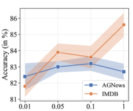
(a) Effect of $\rho$.

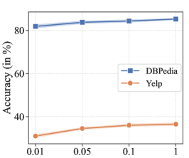
(b) Effect of $\rho$.

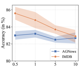
(c) Effect of $\beta$.

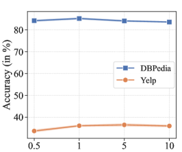
(d) Effect of $\beta$.

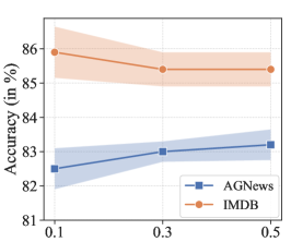
(e) Effect of $\gamma$.

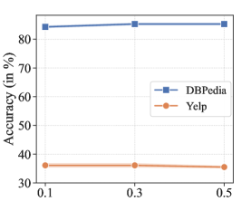
(f) Effect of $\gamma$.

Figure 6: The additional hyperparameter study on the other datasets.

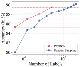
(a) AG News

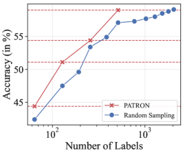
(b) Yelp

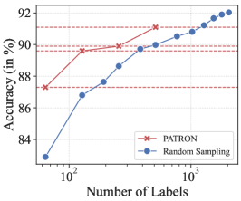
(c) IMDB

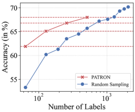
(d) Yahoo!

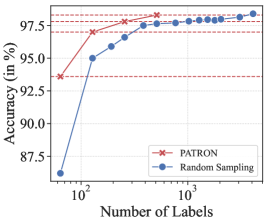
(e) DBPedia.

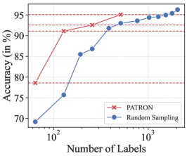
(f) TREC.

Figure 7: Illustration of label efficiency on six datasets.

G.2 Additional Hyperparameter Study

We exhibit the additional hyperparameter study on the other four datasets in Figure 6. Overall, the performance of Patron is stable across a broad range of hyperparameters on all datasets.

G.3 Additional Label Efficiency Study

We provide the label efficiency studies for each dataset in detail, shown in Figure 7. From the figure, we estimate the approximate number of labels required (via random sampling) to achieve the same performance as Patron with 512 labels (Figure 3) as follows: Yahoo: 1280 (2.5X), TREC: 1024 (2X), AG News: 1536 (3X), IMDB: 1024 (2X), DBPedia: 2304 (4.5X), Yelp: 1792 (3.5X). The results indicate that Patron can improve the label efficiency for all datasets significantly.

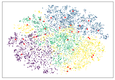
(a) Patron before Ptr.

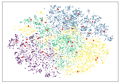
(b) Patron after Ptr.

Figure 8: Illustration of Patron on AG News Dataset. Different colors stands for different classes. Our selected samples are denoted as red triangles.

Appendix H Case Study

Figure 8 gives an example on the selected samples of Patron on AG News dataset. We can see that the initialized solution after Eq. 8 still suffers from the issue of limited coverage, and some of the samples are very close. Fortunately, after the Ptr step, the diversity of selected samples is much improved. This result suggests the Ptr has successfully fulfilled its purpose for diversity-promoting selection.

References

- Aharoni and Goldberg (2020) Roee Aharoni and Yoav Goldberg. 2020. Unsupervised domain clusters in pretrained language models. In Proceedings of the 58th Annual Meeting of the Association for Computational Linguistics, pages 7747–7763, Online. Association for Computational Linguistics.
- Akiba et al. (2019) Takuya Akiba, Shotaro Sano, Toshihiko Yanase, Takeru Ohta, and Masanori Koyama. 2019. Optuna: A next-generation hyperparameter optimization framework. In Proceedings of the 25th ACM SIGKDD International Conference on Knowledge Discovery & Data Mining, KDD ’19, page 2623–2631.
- Ash et al. (2020) Jordan T. Ash, Chicheng Zhang, Akshay Krishnamurthy, John Langford, and Alekh Agarwal. 2020. Deep batch active learning by diverse, uncertain gradient lower bounds. In International Conference on Learning Representations.
- Bragg et al. (2021) Jonathan Bragg, Arman Cohan, Kyle Lo, and Iz Beltagy. 2021. Flex: Unifying evaluation for few-shot nlp. Advances in Neural Information Processing Systems, 34.
- Brown et al. (2020) Tom Brown, Benjamin Mann, Nick Ryder, Melanie Subbiah, Jared D Kaplan, Prafulla Dhariwal, Arvind Neelakantan, Pranav Shyam, Girish Sastry, Amanda Askell, et al. 2020. Language models are few-shot learners. Advances in neural information processing systems, 33:1877–1901.
- Chang et al. (2021) Ernie Chang, Xiaoyu Shen, Hui-Syuan Yeh, and Vera Demberg. 2021. On training instance selection for few-shot neural text generation. In Proceedings of the 59th Annual Meeting of the Association for Computational Linguistics and the 11th International Joint Conference on Natural Language Processing (Volume 2: Short Papers), pages 8–13, Online. Association for Computational Linguistics.
- Chen et al. (2021) Si Chen, Tianhao Wang, and Ruoxi Jia. 2021. Zero-round active learning. arXiv preprint arXiv:2107.06703.
- Chen and Tian (2019) Xinyun Chen and Yuandong Tian. 2019. Learning to perform local rewriting for combinatorial optimization. Advances in Neural Information Processing Systems, 32.
- Clark et al. (2020) Kevin Clark, Minh-Thang Luong, Quoc V. Le, and Christopher D. Manning. 2020. Electra: Pre-training text encoders as discriminators rather than generators. In International Conference on Learning Representations.
- Devlin et al. (2019) Jacob Devlin, Ming-Wei Chang, Kenton Lee, and Kristina Toutanova. 2019. BERT: Pre-training of deep bidirectional transformers for language understanding. In Proceedings of the 2019 Conference of the North American Chapter of the Association for Computational Linguistics: Human Language Technologies, Volume 1 (Long and Short Papers), pages 4171–4186, Minneapolis, Minnesota. Association for Computational Linguistics.
- Ding et al. (2022) Ning Ding, Shengding Hu, Weilin Zhao, Yulin Chen, Zhiyuan Liu, Haitao Zheng, and Maosong Sun. 2022. OpenPrompt: An open-source framework for prompt-learning. In Proceedings of the 60th Annual Meeting of the Association for Computational Linguistics: System Demonstrations, pages 105–113, Dublin, Ireland. Association for Computational Linguistics.
- Du et al. (2021) Jingfei Du, Edouard Grave, Beliz Gunel, Vishrav Chaudhary, Onur Celebi, Michael Auli, Veselin Stoyanov, and Alexis Conneau. 2021. Self-training improves pre-training for natural language understanding. In Proceedings of the 2021 Conference of the North American Chapter of the Association for Computational Linguistics: Human Language Technologies, pages 5408–5418. Association for Computational Linguistics.
- Ein-Dor et al. (2020) Liat Ein-Dor, Alon Halfon, Ariel Gera, Eyal Shnarch, Lena Dankin, Leshem Choshen, Marina Danilevsky, Ranit Aharonov, Yoav Katz, and Noam Slonim. 2020. Active Learning for BERT: An Empirical Study. In Proceedings of the 2020 Conference on Empirical Methods in Natural Language Processing (EMNLP), pages 7949–7962. Association for Computational Linguistics.
- Gao et al. (2021a) Tianyu Gao, Adam Fisch, and Danqi Chen. 2021a. Making pre-trained language models better few-shot learners. In Proceedings of the 59th Annual Meeting of the Association for Computational Linguistics and the 11th International Joint Conference on Natural Language Processing (Volume 1: Long Papers), pages 3816–3830, Online. Association for Computational Linguistics.
- Gao et al. (2021b) Tianyu Gao, Xingcheng Yao, and Danqi Chen. 2021b. SimCSE: Simple contrastive learning of sentence embeddings. In Proceedings of the 2021 Conference on Empirical Methods in Natural Language Processing, pages 6894–6910, Online and Punta Cana, Dominican Republic. Association for Computational Linguistics.
- Gardner et al. (2020) Matt Gardner, Yoav Artzi, Victoria Basmov, Jonathan Berant, Ben Bogin, Sihao Chen, Pradeep Dasigi, Dheeru Dua, et al. 2020. Evaluating models’ local decision boundaries via contrast sets. In Findings of the Association for Computational Linguistics: EMNLP 2020, pages 1307–1323, Online. Association for Computational Linguistics.
- Hacohen et al. (2022) Guy Hacohen, Avihu Dekel, and Daphna Weinshall. 2022. Active learning on a budget: Opposite strategies suit high and low budgets. In Proceedings of the 39th International Conference on Machine Learning, Proceedings of Machine Learning Research, pages 8175–8195. PMLR.
- Hu et al. (2019) Peiyun Hu, Zack Lipton, Anima Anandkumar, and Deva Ramanan. 2019. Active learning with partial feedback. In International Conference on Learning Representations.
- Hu et al. (2022) Shengding Hu, Ning Ding, Huadong Wang, Zhiyuan Liu, Jingang Wang, Juanzi Li, Wei Wu, and Maosong Sun. 2022. Knowledgeable prompt-tuning: Incorporating knowledge into prompt verbalizer for text classification. In Proceedings of the 60th Annual Meeting of the Association for Computational Linguistics (Volume 1: Long Papers), pages 2225–2240, Dublin, Ireland. Association for Computational Linguistics.
- Johnson et al. (2019) Jeff Johnson, Matthijs Douze, and Hervé Jégou. 2019. Billion-scale similarity search with gpus. IEEE Transactions on Big Data.
- Karamcheti et al. (2021) Siddharth Karamcheti, Ranjay Krishna, Li Fei-Fei, and Christopher Manning. 2021. Mind your outliers! investigating the negative impact of outliers on active learning for visual question answering. In Proceedings of the 59th Annual Meeting of the Association for Computational Linguistics and the 11th International Joint Conference on Natural Language Processing (Volume 1: Long Papers), pages 7265–7281, Online. Association for Computational Linguistics.
- Kaushik et al. (2020) Divyansh Kaushik, Eduard Hovy, and Zachary Lipton. 2020. Learning the difference that makes a difference with counterfactually-augmented data. In International Conference on Learning Representations.
- Lehmann et al. (2015) Jens Lehmann, Robert Isele, Max Jakob, Anja Jentzsch, Dimitris Kontokostas, Pablo N Mendes, Sebastian Hellmann, Mohamed Morsey, Patrick Van Kleef, Sören Auer, et al. 2015. Dbpedia–a large-scale, multilingual knowledge base extracted from wikipedia. Semantic web, 6(2):167–195.
- Lewis and Gale (1994) David D Lewis and William A Gale. 1994. A sequential algorithm for training text classifiers. In Proceedings of the 17th annual international ACM SIGIR conference on Research and development in information retrieval, pages 3–12.
- Li et al. (2020) Bohan Li, Hao Zhou, Junxian He, Mingxuan Wang, Yiming Yang, and Lei Li. 2020. On the sentence embeddings from pre-trained language models. In Proceedings of the 2020 Conference on Empirical Methods in Natural Language Processing (EMNLP), pages 9119–9130, Online. Association for Computational Linguistics.
- Li and Roth (2002) Xin Li and Dan Roth. 2002. Learning question classifiers. In The 19th International Conference on Computational Linguistics.
- Liu et al. (2021a) Jiachang Liu, Dinghan Shen, Yizhe Zhang, Bill Dolan, Lawrence Carin, and Weizhu Chen. 2021a. What makes good in-context examples for gpt-? arXiv preprint arXiv:2101.06804.
- Liu et al. (2021b) Pengfei Liu, Weizhe Yuan, Jinlan Fu, Zhengbao Jiang, Hiroaki Hayashi, and Graham Neubig. 2021b. Pre-train, prompt, and predict: A systematic survey of prompting methods in natural language processing. arXiv preprint arXiv:2107.13586.
- Liu et al. (2019) Yinhan Liu, Myle Ott, Naman Goyal, Jingfei Du, Mandar Joshi, Danqi Chen, Omer Levy, Mike Lewis, Luke Zettlemoyer, and Veselin Stoyanov. 2019. Roberta: A robustly optimized bert pretraining approach. arXiv preprint arXiv:1907.11692.
- Loshchilov and Hutter (2019) Ilya Loshchilov and Frank Hutter. 2019. Decoupled weight decay regularization. In International Conference on Learning Representations.
- Maas et al. (2011) Andrew L. Maas, Raymond E. Daly, Peter T. Pham, Dan Huang, Andrew Y. Ng, and Christopher Potts. 2011. Learning word vectors for sentiment analysis. In Proceedings of the 49th Annual Meeting of the Association for Computational Linguistics: Human Language Technologies, pages 142–150, Portland, Oregon, USA. Association for Computational Linguistics.
- Margatina et al. (2022) Katerina Margatina, Loic Barrault, and Nikolaos Aletras. 2022. On the importance of effectively adapting pretrained language models for active learning. In Proceedings of the 60th Annual Meeting of the Association for Computational Linguistics (Volume 2: Short Papers), pages 825–836, Dublin, Ireland. Association for Computational Linguistics.
- Margatina et al. (2021) Katerina Margatina, Giorgos Vernikos, Loïc Barrault, and Nikolaos Aletras. 2021. Active learning by acquiring contrastive examples. In Proceedings of the 2021 Conference on Empirical Methods in Natural Language Processing, pages 650–663, Online and Punta Cana, Dominican Republic. Association for Computational Linguistics.
- Meng et al. (2019) Yu Meng, Jiaming Shen, Chao Zhang, and Jiawei Han. 2019. Weakly-supervised hierarchical text classification. In Proceedings of the AAAI conference on artificial intelligence, volume 33, pages 6826–6833.
- Meng et al. (2020) Yu Meng, Yunyi Zhang, Jiaxin Huang, Chenyan Xiong, Heng Ji, Chao Zhang, and Jiawei Han. 2020. Text classification using label names only: A language model self-training approach. In Proceedings of the 2020 Conference on Empirical Methods in Natural Language Processing (EMNLP), pages 9006–9017. Association for Computational Linguistics.
- Min et al. (2022) Sewon Min, Mike Lewis, Hannaneh Hajishirzi, and Luke Zettlemoyer. 2022. Noisy channel language model prompting for few-shot text classification. In Proceedings of the 60th Annual Meeting of the Association for Computational Linguistics (Volume 1: Long Papers), pages 5316–5330, Dublin, Ireland. Association for Computational Linguistics.
- Müller et al. (2022) Thomas Müller, Guillermo Pérez-Torró, Angelo Basile, and Marc Franco-Salvador. 2022. Active few-shot learning with fasl. arXiv preprint arXiv:2204.09347.
- Park et al. (2022) Chanho Park, Rehan Ahmad, and Thomas Hain. 2022. Unsupervised data selection for speech recognition with contrastive loss ratios. In ICASSP 2022-2022 IEEE International Conference on Acoustics, Speech and Signal Processing (ICASSP), pages 8587–8591. IEEE.
- Raffel et al. (2020) Colin Raffel, Noam Shazeer, Adam Roberts, Katherine Lee, Sharan Narang, Michael Matena, Yanqi Zhou, Wei Li, and Peter J Liu. 2020. Exploring the limits of transfer learning with a unified text-to-text transformer. Journal of Machine Learning Research, 21:1–67.
- Schick and Schütze (2021a) Timo Schick and Hinrich Schütze. 2021a. Exploiting cloze-questions for few-shot text classification and natural language inference. In Proceedings of the 16th Conference of the European Chapter of the Association for Computational Linguistics: Main Volume, pages 255–269, Online. Association for Computational Linguistics.
- Schick and Schütze (2021b) Timo Schick and Hinrich Schütze. 2021b. It’s not just size that matters: Small language models are also few-shot learners. In Proceedings of the 2021 Conference of the North American Chapter of the Association for Computational Linguistics: Human Language Technologies, pages 2339–2352, Online. Association for Computational Linguistics.
- Scholkopf et al. (1997) Bernhard Scholkopf, Kah-Kay Sung, Christopher JC Burges, Federico Girosi, Partha Niyogi, Tomaso Poggio, and Vladimir Vapnik. 1997. Comparing support vector machines with gaussian kernels to radial basis function classifiers. IEEE transactions on Signal Processing, 45(11):2758–2765.
- Schröder et al. (2022) Christopher Schröder, Andreas Niekler, and Martin Potthast. 2022. Revisiting uncertainty-based query strategies for active learning with transformers. In Findings of the Association for Computational Linguistics: ACL 2022, pages 2194–2203, Dublin, Ireland. Association for Computational Linguistics.
- Sener and Savarese (2018) Ozan Sener and Silvio Savarese. 2018. Active learning for convolutional neural networks: A core-set approach. In International Conference on Learning Representations.
- Settles (2011) Burr Settles. 2011. From theories to queries: Active learning in practice. In Active Learning and Experimental Design workshop, pages 1–18. JMLR Workshop and Conference Proceedings.
- Shen et al. (2021) Jiaming Shen, Jialu Liu, Tianqi Liu, Cong Yu, and Jiawei Han. 2021. Training ELECTRA augmented with multi-word selection. In Findings of the Association for Computational Linguistics: ACL-IJCNLP 2021, pages 2475–2486, Online. Association for Computational Linguistics.
- Shnarch et al. (2022) Eyal Shnarch, Ariel Gera, Alon Halfon, Lena Dankin, Leshem Choshen, Ranit Aharonov, and Noam Slonim. 2022. Cluster & tune: Boost cold start performance in text classification. In Proceedings of the 60th Annual Meeting of the Association for Computational Linguistics (Volume 1: Long Papers), pages 7639–7653, Dublin, Ireland. Association for Computational Linguistics.
- Socher et al. (2013) Richard Socher, Alex Perelygin, Jean Wu, Jason Chuang, Christopher D. Manning, Andrew Ng, and Christopher Potts. 2013. Recursive deep models for semantic compositionality over a sentiment treebank. In Proceedings of the 2013 Conference on Empirical Methods in Natural Language Processing, pages 1631–1642. Association for Computational Linguistics.
- Su et al. (2022) Hongjin Su, Jungo Kasai, Chen Henry Wu, Weijia Shi, Tianlu Wang, Jiayi Xin, Rui Zhang, Mari Ostendorf, Luke Zettlemoyer, Noah A Smith, et al. 2022. Selective annotation makes language models better few-shot learners. arXiv preprint arXiv:2209.01975.
- Tam et al. (2021) Derek Tam, Rakesh R. Menon, Mohit Bansal, Shashank Srivastava, and Colin Raffel. 2021. Improving and simplifying pattern exploiting training. In Proceedings of the 2021 Conference on Empirical Methods in Natural Language Processing, pages 4980–4991, Online and Punta Cana, Dominican Republic. Association for Computational Linguistics.
- Vinh et al. (2010) Nguyen Xuan Vinh, Julien Epps, and James Bailey. 2010. Information theoretic measures for clusterings comparison: Variants, properties, normalization and correction for chance. The Journal of Machine Learning Research, 11:2837–2854.
- Wang et al. (2021a) Xudong Wang, Long Lian, and Stella X Yu. 2021a. Unsupervised data selection for data-centric semi-supervised learning. arXiv preprint arXiv:2110.03006.
- Wang et al. (2021b) Yaqing Wang, Subhabrata Mukherjee, Xiaodong Liu, Jing Gao, Ahmed Hassan Awadallah, and Jianfeng Gao. 2021b. List: Lite self-training makes efficient few-shot learners. arXiv preprint arXiv:2110.06274.
- Wolf et al. (2020) Thomas Wolf, Lysandre Debut, Victor Sanh, Julien Chaumond, Clement Delangue, Anthony Moi, Pierric Cistac, Tim Rault, et al. 2020. Transformers: State-of-the-art natural language processing. In Proceedings of the 2020 Conference on Empirical Methods in Natural Language Processing: System Demonstrations, pages 38–45, Online. Association for Computational Linguistics.
- Xia et al. (2022) Mengzhou Xia, Mikel Artetxe, Jingfei Du, Danqi Chen, and Ves Stoyanov. 2022. Prompting electra: Few-shot learning with discriminative pre-trained models. arXiv preprint arXiv:2205.15223.
- Xie et al. (2020) Qizhe Xie, Zihang Dai, Eduard Hovy, Thang Luong, and Quoc Le. 2020. Unsupervised data augmentation for consistency training. Advances in Neural Information Processing Systems, 33.
- Xu et al. (2023) Ran Xu, Yue Yu, Hejie Cui, Xuan Kan, Yanqiao Zhu, Joyce C. Ho, Chao Zhang, and Carl Yang. 2023. Neighborhood-regularized self-training for learning with few labels. In Proceedings of the Thirty-Seventh AAAI Conference on Artificial Intelligence.
- Yao et al. (2022) Yuan Yao, Bowen Dong, Ao Zhang, Zhengyan Zhang, Ruobing Xie, Zhiyuan Liu, Leyu Lin, Maosong Sun, and Jianyong Wang. 2022. Prompt tuning for discriminative pre-trained language models. In Findings of the Association for Computational Linguistics: ACL 2022, pages 3468–3473, Dublin, Ireland. Association for Computational Linguistics.
- Yu et al. (2022) Yue Yu, Lingkai Kong, Jieyu Zhang, Rongzhi Zhang, and Chao Zhang. 2022. AcTune: Uncertainty-based active self-training for active fine-tuning of pretrained language models. In Proceedings of the 2022 Conference of the North American Chapter of the Association for Computational Linguistics: Human Language Technologies, pages 1422–1436, Seattle, United States. Association for Computational Linguistics.
- Yu et al. (2021) Yue Yu, Simiao Zuo, Haoming Jiang, Wendi Ren, Tuo Zhao, and Chao Zhang. 2021. Fine-tuning pre-trained language model with weak supervision: A contrastive-regularized self-training approach. In Proceedings of the 2021 Conference of the North American Chapter of the Association for Computational Linguistics: Human Language Technologies, pages 1063–1077, Online. Association for Computational Linguistics.
- Yuan et al. (2020) Michelle Yuan, Hsuan-Tien Lin, and Jordan Boyd-Graber. 2020. Cold-start active learning through self-supervised language modeling. In Proceedings of the 2020 Conference on Empirical Methods in Natural Language Processing (EMNLP), pages 7935–7948, Online. Association for Computational Linguistics.
- Zhang et al. (2022a) Jieyu Zhang, Cheng-Yu Hsieh, Yue Yu, Chao Zhang, and Alexander Ratner. 2022a. A survey on programmatic weak supervision. arXiv preprint arXiv:2202.05433.
- Zhang and Plank (2021) Mike Zhang and Barbara Plank. 2021. Cartography active learning. In Findings of the Association for Computational Linguistics: EMNLP 2021, pages 395–406, Punta Cana, Dominican Republic. Association for Computational Linguistics.
- Zhang et al. (2022b) Ningyu Zhang, Luoqiu Li, Xiang Chen, Shumin Deng, Zhen Bi, Chuanqi Tan, Fei Huang, and Huajun Chen. 2022b. Differentiable prompt makes pre-trained language models better few-shot learners. In International Conference on Learning Representations.
- Zhang et al. (2022c) Rongzhi Zhang, Yue Yu, Pranav Shetty, Le Song, and Chao Zhang. 2022c. Prompt-based rule discovery and boosting for interactive weakly-supervised learning. In Proceedings of the 60th Annual Meeting of the Association for Computational Linguistics (Volume 1: Long Papers), pages 745–758, Dublin, Ireland. Association for Computational Linguistics.
- Zhang et al. (2020a) Rongzhi Zhang, Yue Yu, and Chao Zhang. 2020a. SeqMix: Augmenting active sequence labeling via sequence mixup. In Proceedings of the 2020 Conference on Empirical Methods in Natural Language Processing (EMNLP), pages 8566–8579, Online. Association for Computational Linguistics.
- Zhang et al. (2020b) Tianyi Zhang, Felix Wu, Arzoo Katiyar, Kilian Q Weinberger, and Yoav Artzi. 2020b. Revisiting few-sample bert fine-tuning. arXiv preprint arXiv:2006.05987.
- Zhang et al. (2015) Xiang Zhang, Junbo Zhao, and Yann LeCun. 2015. Character-level convolutional networks for text classification. Advances in neural information processing systems, 28:649–657.
- Zhao et al. (2021) Zihao Zhao, Eric Wallace, Shi Feng, Dan Klein, and Sameer Singh. 2021. Calibrate before use: Improving few-shot performance of language models. In International Conference on Machine Learning, pages 12697–12706. PMLR.