Discrete and continuous dynamics of real $3$-dimensional nilpotent polynomial vector fields

Abstract.

A large class of real $3$-dimensional nilpotent polynomial vector fields of arbitrary degree is considered. The aim of this work is to present general properties of the discrete and continuous dynamical systems induced by these vector fields. In the discrete case, it is proved that each dynamical system has a unique fixed point and no $2$-cycles. Moreover, either the fixed point is a global attractor or there exists a $3$-cycle which is not a repeller. In the continuous setting, it is proved that each dynamical system is polynomially integrable. In addition, for a subclass of the considered vector fields, the system is polynomially completely integrable. Furthermore, for a family of low degree vector fields, it is provided a more precise description about the global dynamics of the trajectories of the induced dynamical system. In particular, it is proved the existence of an invariant surface foliated by periodic orbits. Finally, some remarks and open questions, motivated by our results, the Markus–Yamabe Conjecture and the problem of planar limit cycles, are given.

1. Introduction

The study of nilpotent polynomial vector fields, i.e. polynomial vector fields $\displaystyle F\colon\mathbb{K}^{n}\longrightarrow\mathbb{K}^{n}$ whose Jacobian matrix $JF$ is nilpotent, where $\mathbb{K}$ is a field of characteristic zero, is closely related to the Jacobian Conjecture [7, 8]. Indeed, the seminal works of A.V. Yagzhev [16] and H. Bass et al. [1] prove that for analyzing the Jacobian Conjecture is sufficient to focus on polynomial vector fields of the form $I+F$, where $I$ is the identity and $F$ is nilpotent and homogeneous of degree three. Another motivation for studying nilpotent polynomial vector fields arises from dynamics. Recall that each real vector field $F\displaystyle\colon\mathbb{R}^{n}\longrightarrow\mathbb{R}^{n}$ induces a discrete dynamical system defined by the iteration of $F$ and a continuous dynamical system defined by the flow generated by the differential system associated with $F$. For this induced continuous (resp. discrete) dynamical system L. Markus and H. Yamabe [14] (resp. J. LaSalle [13]) established the continuous (resp. discrete) global stability conjecture, which is true for $n\leq 2$ with $F$ polynomial, but it admits counterexamples for $n\geq 3$. Such counterexamples have the form $\lambda I+F$ where $\lambda<0\,(\textrm{resp. }|\lambda|<1)$ and $F$ a nilpotent polynomial vector field, see [5, 6].

Therefore, the nilpotent polynomial vector fields play a fundamental role in order to give a negative or positive answer to the Jacobian Conjecture as well as in the construction of examples and counterexamples to the Markus–Yamabe and LaSalle conjectures. Furthermore, the characterization and understanding of this kind of vector fields in any dimension and any degree, even inhomogeneous, go beyond these conjectures and represent a challenging open problem by itself.

The characterization of nilpotent polynomial vector fields is well-known in dimension two [7, p. 148]. In dimension three, it depends on the linear dependence of the components of $F$ over $\mathbb{K}$. When the components are linearly dependent, it is given in [4, Corollary 1.1] (the former counterexamples to both Markus–Yamabe and LaSalle conjectures have linearly dependent components). When the components are linearly independent, the first steps towards such a characterization were taken by M. Chamberland and A. van den Essen in [4]. In particular, they prove in [4, Theorem 2.1] that any polynomial vector field $F(x,y,z)=(u(x,y),v(x,y,z),h(u(x,y)))$ is nilpotent if and only if

$$F(x,y,z)=\left(g(y+b(x)),v_{1}z-(b_{1}+2v_{1}\alpha x)g(y+b(x)),\alpha(g(y+b(x)))^{2}\right),$$

where $b(x)=b_{1}x+v_{1}\alpha x^{2}$, $v_{1}\alpha\neq 0$ and $g\in\mathbb{K}[t]$, with $\deg g\geq 1$ and $g(0)=0$. Later, Chamberland consider the above form of $F$ with the particular parameters: $b_{1}=0,v_{1}=1$ and $\alpha=-1$. He showed in [3] that the discrete dynamical system induced by such a particular vector field has a unique fixed point, there are not 2-cycles, and under a suitable condition on the function $g$ there exists a $3$-cycle, which show that the nilpotent polynomial vector fields can induce a rich dynamics.

Another step in the task of the characterization of nilpotent polynomial vector fields in dimension three has been done by D. Yan and G. Tang in [18], where they generalize the results of [4]. This characterization problem has been followed by several authors; see for instance [17] and references there in. One of the most recent and general results in this issue is [2, Theorem 1], which gives the characterization of all nilpotent polynomial vector fields $\displaystyle F\colon\mathbb{K}^{n}\longrightarrow\mathbb{K}^{n}$ of the form

$$F(x_{1},x_{2},\ldots,x_{n})=(F_{1}(x_{1},x_{2}),F_{2}(x_{1},x_{2},x_{3}),\ldots,F_{n-1}(x_{1},x_{2},x_{n}),F_{n}(x_{1},x_{2})).$$

In the three dimensional real case and by changing the variables $x_{1},x_{2},x_{3}$ by $x,y,z$, such a characterization is as follows. The polynomial vector field

(1) $$F\colon\mathbb{R}^{3}\longrightarrow\mathbb{R}^{3},\;(x,y,z)\longmapsto(F_{1}(x,y),F_{2}(x,y,z),F_{3}(x,y)),$$

is nilpotent if and only if

(2) $$F_{1}(x,y) =P_{1}\big{(}y+A_{1}(x)\big{)},$$

$$F_{2}(x,y,z) =P_{2}\Big{(}z+\frac{1}{d_{2}p_{d_{2}}}A_{2}(x)\Big{)}-A_{1}^{\prime}(x)F_{1}(x,y),$$

$$F_{3}(x,y) =-\frac{1}{d_{2}{p_{d}}_{2}}\left[-\frac{1}{2}{A_{1}^{\prime\prime}(x)}\big{(}F_{1}(x,y)\big{)}^{2}+A_{2}^{\prime}(x)F_{1}(x,y)\right]+A_{3},$$

where

(3) $$\left\{\begin{aligned} &P_{i}\in\mathbb{R}[s],\;d_{i}:=\deg P_{i}\geq 1,\;p_{d_{i}}:=\mbox{the leading coefficient of $P_{i}$},\\ &A_{1}(x)=a_{10}+a_{11}x+a_{12}x^{2},\,\,A_{2}(x)=a_{20}+a_{21}x,\>A_{3}\in\mathbb{R}.\\ &\textrm{If}\,\,d_{2}>1,\,\,then\,\,A_{1}^{\prime\prime}(x)\equiv 0.\end{aligned}\right.$$

In this work, inspired by Chamberland’s article [3], we will analyze the discrete and continuous dynamics induced by the nilpotent polynomial vector fields (1), whose components are in (2). More precisely, on the one hand, we will study the discrete dynamical system $(\mathbb{R}^{3},\mathbb{N}_{0},F)$, where the dynamics is given by

(4) $${x}_{k+1} =F_{1}\left(x_{k},y_{k}\right),$$

$${y}_{k+1} =F_{2}\left(x_{k},y_{k},z_{k}\right),$$

$${z}_{k+1} =F_{3}\left(x_{k},y_{k}\right).$$

On the other hand, the continuous dynamical system $(\mathbb{R}^{3},\mathbb{R},\Phi)$, where $\Phi$ is the flow generated by the differential system

(5) $$\dot{x} =F_{1}(x,y),$$

$$\dot{y} =F_{2}(x,y,z),$$

$$\dot{z} =F_{3}(x,y).$$

Concerning the discrete dynamics our main result is the following.

Theorem 1.1.

Each system (4) has a unique fixed point and there are no $2$-cycles. In addition,

1. if $\deg A_{1}(x)=1$, then the fixed point is a global attractor, which is reached from any initial point after three iterations;

2. if $\deg A_{1}(x)=2$, then the system has a $3$-cycle which is not a repeller.

Although the assertions of this result are essentially the same as in the work of Chamberland [3, Theorem 3.1], we emphasize that the above theorem is a generalization. Indeed, the family of nilpotent vector fields of the form (1) is wider than the studied in [3]. For instance, the polynomial $P_{2}(s)$ in (2) is of arbitrary degree while in Chamberland’s paper is linear.

Regarding the continuous dynamics our main result is as follows.

Theorem 1.2.

Each differential system (5) is polynomially integrable. In addition, if $\deg A_{1}(x)=1$, then differential system (5) is polynomially completely integrable.

This result gives valuable information to describe and comprehend the long-term behavior of the trajectories of each differential system (5). In particular, it says that the dynamics of the system occurs in the algebraic surfaces defined by the level sets of the polynomial first integral guaranteed by the theorem. Thus, the topology of these surfaces plays an important role in kind of orbits that they can supported. For instance, if they are simply connected surfaces and does not posses any singularity of the system, then they can not support periodic orbits of the differential system.

In order to get more precise features on the dynamics of the trajectories of these continuous dynamical systems, we will study some particular cases according with the degrees of $P_{1}(s)$ and $P_{2}(s)$ in (3). Thus, we have the following result.

Proposition 1.3.

Assume that $\deg P_{1}(s)=\deg P_{2}(s)=1$ in system (5).

1. If $\deg A_{1}(x)=1$, then each nontrivial trajectory of system (5) goes to infinity in forward and backward time.

2. If $\deg A_{1}(x)=2$ and we define $\mu:=A_{3}\,a_{12}\,p_{d_{2}}\,p_{d_{1}}^{2}$, then

   1. each trajectory of (5) goes to infinity in forward and backward time if $\mu>0$,

   2. there exists a unique cuspidal invariant surface $\mathcal{S}_{0}$ of (5) and each trajectory of (5) in $\mathbb{R}^{3}\backslash\mathcal{S}_{0}$ goes to infinity in forward and backward time if $\mu=0$,

   3. there exists a unique isochronous periodic surface $\mathcal{S}_{\mu}$ of (5) and each trajectory of (5) in $\mathbb{R}^{3}\backslash\mathcal{S}_{\mu}$ goes to infinity in forward and backward time if $\mu<0$.

The properties of statement $2)$ of this proposition states an interesting and surprising analogy with the Bogdanov–Takens bifurcation. Indeed, in such a bifurcation, we can choose a $1$-parameter curve in such a way that the corresponding system has no singularities for positive values of the parameter, a cusp singularity if the parameter is zero, and a unique periodic orbit (limit cycle) for negative values of the parameter. See [12, p. 324].

The paper is organized as follows. In Section 2 we will simplify the expression of dynamical systems (4) and (5) through polynomial automorphisms. We use the simplified expressions to analyze the discrete dynamics in Section 3 and the continuous dynamics in Section 4. Some concluding remarks, questions and comments are given in Section 5.

2. Simpler conjugated systems

The main idea to prove our results is the use of polynomial automorphisms of $\mathbb{R}^{3}$ to transform the original dynamical systems into new ones with simpler expressions. The transformed dynamical systems are analyzed easily. Concretely, the polynomial map

(6)

is a polynomial automorphism of $\displaystyle\mathbb{R}^{3}$, whose inverse is

(7)

If we define $\displaystyle G(u,v,w):=(\Psi^{-1}\circ F\circ\Psi)(u,v,w)$, then $\displaystyle(\mathbb{R}^{n},\mathbb{N}_{0},F)$ and $\displaystyle(\mathbb{R}^{n},\mathbb{N}_{0},G)$ are conjugated. Explicitly, by using equations (2), (3), (6), and (7), the discrete dynamical system (4) is conjugated to the system

(8) $${u}_{k+1} =P_{1}\left(v_{k}\right),$$

$${v}_{k+1} =P_{2}\left(w_{k}\right)+a_{12}P_{1}\left(v_{k}\right)\Big{(}P_{1}\left(v_{k}\right)-2u_{k}\Big{)}+a_{10},$$

$${w}_{k+1} =\frac{a_{12}}{d_{2}p_{d_{2}}}\big{(}P_{1}(v_{k})\big{)}^{2}+A_{3}+\frac{a_{20}}{d_{2}p_{d_{2}}}.$$

Analogously, by using (7), as a change of coordinates, together with equations (2) and (3), the differential system (5) becomes

(9) $$\dot{u} =P_{1}(v),$$

$$\dot{v} =P_{2}(w),$$

$$\dot{w} =\frac{a_{12}}{d_{2}{p_{d}}_{2}}\big{(}P_{1}(v)\big{)}^{2}+A_{3}.$$

Thus, the continuous dynamical systems associated with differential systems $\eqref{sistema-diferencial-3d}$ and (9) are conjugated.

3. Discrete dynamics

In this section, we will prove the general properties of the discrete dynamical system (4) stated in Theorem 1.1.

Proof of Theorem 1.1.

From previous section, we know that the discrete dynamical systems (4) and (8) are conjugated. Hence, we will use system (8) to give the proof of the theorem. The general part of the result will be proved by considering two cases: $d_{2}>1$ and $d_{2}=1$. In addition, the proof of Statements $1)$ and $2)$ will be provided in the first and second cases, respectively.

Case 1: $d_{2}>1$. Taking in account (3), $a_{12}=0$. So system (8) is simplified. Thus, its fixed points are the solutions to the algebraic system

$$u=P_{1}\left(v\right),\quad v=P_{2}\left(w\right)+a_{10},\quad w=A_{3}+\frac{a_{20}}{d_{2}p_{d_{2}}},$$

which has the unique solution

$$(u_{0},v_{0},w_{0})=\left(P_{1}\left(v_{0}\right),P_{2}\left(w_{0}\right)+a_{10},A_{3}+\frac{a_{20}}{d_{2}p_{d_{2}}}\right).$$

Moreover, if $(u,v,w)$ was part of a $2$-cycle, then

$$u=P_{1}\big{(}P_{2}\left(w\right)+a_{10}\big{)},\quad v=P_{2}\Big{(}A_{3}+\frac{a_{20}}{d_{2}p_{d_{2}}}\Big{)}+a_{10},\quad{w}=A_{3}+\frac{a_{20}}{d_{2}p_{d_{2}}}.$$

Hence $(u,v,w)=(u_{0},v_{0},w_{0})$, the fixed point, so there are no $2$-cycles in this case. Even more, the third iteration $(u_{3},v_{3},w_{3})$ of an arbitrary point $(u,v,w)$ is

$$(u_{3},v_{3},w_{3})=\bigg{(}P_{1}\Big{(}P_{2}\Big{(}A_{3}+\frac{a_{20}}{d_{2}p_{d_{2}}}\Big{)}+a_{10}\Big{)},P_{2}\Big{(}A_{3}+\frac{a_{20}}{d_{2}p_{d_{2}}}\Big{)}+a_{10},A_{3}+\frac{a_{20}}{d_{2}p_{d_{2}}}\bigg{)},$$

which clearly does not depend on the coordinates of the initial point $(u,v,w)$. The point $(u_{3},v_{3},w_{3})$ is precisely the fixed point $(u_{0},v_{0},w_{0})$. This last argument is the proof of Statement 1) because $a_{21}=0$ is equivalent to $\deg A_{1}(x)=1$.

Case 2: $d_{2}=1$. We assume $P_{2}(s)=p_{21}s+p_{20}$, and define $\alpha:=p_{20}+a_{10}$. Moreover, we can assume $\deg A_{1}(x)=2$ because otherwise we are in the previous paragraph. The polynomial map

is a polynomial automorphism of $\mathbb{R}^{3}$ that gives

$$(\Psi_{2}^{-1}\circ G\circ\Psi_{2})(X,Y,Z)=\Big{(}P_{1}(Y)-P_{1}(Z),\,Z,\,a_{12}\big{(}P_{1}(Y)-P_{1}(Z)\big{)}^{2}+\nu\Big{)},$$

where $\nu:=p_{21}A_{3}+a_{20}+\alpha$. Thus, system (4) is also conjugated to the system

(10) $${X}_{k+1} =P_{1}(Y_{k})-P_{1}(Z_{k}),$$

$${Y}_{k+1} =Z_{k},$$

$${Z}_{k+1} =a_{12}\big{(}P_{1}(Y_{k})-P_{1}(Z_{k})\big{)}^{2}+\nu.$$

From second equation in (10) it follows that this last discrete dynamical system has a unique fixed point at $(X_{0},Y_{0},Z_{0})=(0,\nu,\nu)$. Moreover, if $(X,Y,Z)$ was part of a $2$-cycle, then

$${X}=P_{1}(Z)-P_{1}(Y),\quad{Y}=a_{12}X^{2}+\nu,\quad{Z}=a_{12}X^{2}+\nu.$$

Hence $(X,Y,Z)=(0,\nu,\nu)$, so there are no $2$-cycles. This completes the proof of the general part of the theorem. To finish, we will prove Statement 2).

We claim that if the equation

(11) $$a_{12}\big{(}P_{1}(s)-P_{1}(\nu)\big{)}^{2}+\nu=s$$

has a real solution $s_{0}\neq\nu$, then the point $(0,s_{0},\nu)$ is part of a $3$-cycle of the discrete dynamical system (10). Indeed, if (11) holds for $s_{0}\neq\nu$, then

$$(0,s_{0},\nu)\longrightarrow\big{(}P_{1}(s_{0})-P_{1}(\nu),\nu,s_{0})\big{)}\longrightarrow\big{(}P_{1}(\nu)-P_{1}(s_{0}),s_{0},s_{0})\big{)}\longrightarrow(0,s_{0},\nu),$$

which is a $3$-cycle because no one of these points is the fixed point. Look for a solution of equation (11) is equivalent to look for a zero of the polynomial

(12) $$h(s)=a_{12}\big{(}P_{1}(s)-P_{1}(\nu)\big{)}^{2}+\nu-s.$$

Since $h(s)$ has even degree and it has a simple zero at $s=\nu$ because $h(\nu)=0$ and $h^{\prime}(\nu)=-1$, it must have another real zero. Therefore, our claim follows.

The linearization of (10) at an arbitrary point $(X,Y,Z)$ is the matrix

$$\begin{pmatrix}0&P_{1}^{\prime}(Y)&-P_{1}^{\prime}(Z)\\ 0&0&1\\ 0&2\,a_{12}(P_{1}(Y)-P_{1}(Z))P_{1}^{\prime}(Y)&-2\,a_{12}(P_{1}(Y)-P_{1}(Z))P_{1}^{\prime}(Z)\end{pmatrix}.$$

By evaluating this matrix at each one of the three points of the $3$-cycle and computing their product we obtain the linearization of the third iteration of (10) at the point $(0,s_{0},\nu),$ which after using that $(P_{1}(s_{0})-P_{1}(\nu))^{2}=(s_{0}-\nu)/a_{12}$ can be written as

$$\begin{pmatrix}0&*&*\\ 0&L_{22}&*\\ 0&0&0\end{pmatrix}$$

where $L_{22}:=4a_{12}^{2}\big{(}P_{1}(s_{0})-P_{1}(\nu)\big{)}^{2}(P_{1}^{{}^{\prime}}(s_{0}))^{2}.$ Therefore, the $3$-cycle is an attractor when $|L_{22}|<1$ and it is a saddle when $|L_{22}|>1$. ∎

Remark 3.1.

When $P_{1}(s)$ is linear the equation (12) has only one solution $s_{0}$, different from $\nu$, and $L_{22}=4.$ Hence, in this case the $3$-cycle of (10) is not an attractor. We can find suitable $a_{12},\nu$ and $P_{1}(s)$ of degree two such that (10) has a $3$-cycle which is attractor.

Remark 3.2.

When $P_{1}(s)$ is linear, we compute, by using computational software, the Gröebner basis of the components of $(\Psi_{2}^{-1}\circ G\circ\Psi_{2})^{5}(X,Y,Z)-(X,Y,Z)$. We obtain three polynomials, one of them depends only on $Z$ and has even degree with $\nu$ as a solution, the other two are linear in $X$ and $Y$. Hence, (10) has a $5$-cycle.

4. Continuous dynamics

In this section, we will prove the general properties of the continuous dynamical system (5). Before that, we need to recall some concepts related to the assertions of Theorem 1.2 and Proposition 1.3.

A non-constant function $H\colon\mathbb{R}^{3}\longrightarrow\mathbb{R}$ is a $C^{r}$ first integral for differential system (5) if the equation

$$\langle F,\nabla H\rangle=F_{1}H_{x}+F_{2}H_{y}+F_{3}H_{z}=0$$

holds on the whole $\mathbb{R}^{3}$ and $H$ is of class $C^{r}$, with $r=1,2,\ldots,\infty,\omega$, where $C^{\omega}$ stands for analytic functions. In addition, if $H$ is a polynomial function, then we have a polynomial first integral. Two $C^{r}$ functions $H_{1}(x,y,z)$ and $H_{2}(x,y,z)$ are functionally independent in $\mathbb{R}^{3}$ if their gradients, $\nabla H_{1}$ and $\nabla H_{2}$, are linearly independent in a full Lebesgue measure subset of $\mathbb{R}^{3}$. Then, by definition, differential system (5) is $C^{r}$(polynomially) integrable if it has a $C^{r}$ (polynomial) first integral in $\mathbb{R}^{3}$. Furthermore, it is $C^{r}$ (polynomially) completely integrable if it has two functionally independent $C^{r}$ (polynomial) first integrals in $\mathbb{R}^{3}$.

Definition 4.1.

A periodic surface of system (5) is a surface $S\subset\mathbb{R}^{3}$, which is foliated by periodic orbits of the system. A periodic surface $S$ of system (5) is isochronous when all its periodic orbits have the same period.

Proof of Theorem 2.

From Section 2, we know that differential systems (5) and (9) are polynomially conjugated through the change of coordinates (7). Moreover, the last two equations in (9) form a planar Hamiltonian system, whose Hamiltonian function is

$$G(v,w):=\int P_{2}(w)\,dw-\frac{a_{12}}{d_{2}{p_{d}}_{2}}\int(P_{1}(v))^{2}\,dv-A_{3}v.$$

Then, by extending this function to $\mathbb{R}^{3}$, that is, by defining the polynomial function

(13) $$H(u,v,w):=\int P_{2}(w)\,dw-\frac{a_{12}}{d_{2}{p_{d}}_{2}}\int(P_{1}(v))^{2}\,dv-A_{3}v,$$

we have

$$H_{u}=0,\quad H_{v}=-\frac{a_{12}}{d_{2}{p_{d}}_{2}}(P_{1}(v))^{2}-A_{3}\quad\mbox{and}\quad H_{w}=P_{2}(w).$$

Thus,

$$P_{1}(v)\,H_{u}+P_{2}(w)\,H_{v}+\left(\frac{a_{12}}{d_{2}{p_{d}}_{2}}\big{(}P_{1}(v)\big{)}^{2}+A_{3}\right)H_{w}=0,\quad\forall\;(u,v,w)\in\mathbb{R}^{3}.$$

Hence, $H$ is a polynomial first integral of system (9). Since the change of variables (7) is polynomial, also differential system (5) has polynomial first integral.

We now prove the second part of the theorem. Since $\deg A_{1}(x)=1$, $a_{12}=0$. Then, system (9) reduces to

(14) $$\dot{u} =P_{1}(v),$$

$$\dot{v} =P_{2}(w),$$

$$\dot{w} =A_{3}.$$

We have proved that system (9) has a polynomial first integral, then we will show the existence of an additional polynomial first integral of the system.

If $A_{3}=0$, then (14) admits the two functionally independent polynomial first integrals

$$H_{1}(u,v,w)=w\quad\mbox{and}\quad H_{2}(u,v,w)=\int P_{1}(v)\,dv-uP_{2}(w).$$

If $A_{3}\neq 0$, then (14) admits the two functionally independent polynomial first integrals

$$H_{1}(u,v,w)=\int P_{2}(w)\,dw-A_{3}v$$

and

$$H_{2}(u,v,w)=A_{3}^{d_{1}+1}u-\sum_{j=0}^{d_{1}}(-1)^{j}A_{3}^{d_{1}-j}\left(\frac{d^{j}}{dv^{j}}P_{1}(v)\right)\,\xi_{j}(w),$$

where $\xi_{0}(w)=w$ and $\xi_{j}(w)=\int P_{2}(w)\xi_{j-1}(w)\,dw$ for $j=1,2,\ldots,d_{1}$. In both previous cases $H_{1}(u,v,w)$ is the reduction of the polynomial first integral (13). Thus, system (14) is polynomially completely integrable. Therefore, system (5), with $\deg A_{1}(x)=1$, is also polynomially completely integrable because it and system (14) are equivalent after a polynomial change of coordinates. ∎

4.1. Case $d_{1}=d_{2}=1$

Proof of Proposition 1.3.

Recall that differential systems (5) and (9) are equivalent under the polynomial change of coordinates (7).

Statement $1)$. Since $\deg A_{1}(x)=1$, $a_{12}=0$. The linear change of coordinates

$$X=\frac{1}{p_{d_{1}}p_{d_{2}}}\,u,\;Y=\frac{1}{p_{d_{1}}p_{d_{2}}}\,P_{1}(v),\;Z=\frac{1}{p_{d_{2}}}\,P_{2}(w)$$

transforms the differential system (9), with $a_{12}=0$, into the differential system

$$\dot{X} =Y,$$

$$\dot{Y} =Z,$$

$$\dot{Z} =A_{3},$$

which can be solved explicitly. Indeed, the trajectory $\phi_{t}(X_{0},Y_{0},Z_{0})$ of the system passing through the point $(X_{0},Y_{0},Z_{0})$ has the components:

$$X(t)=\dfrac{A_{{3}}}{6}\,{t}^{3}+\frac{Z_{{0}}}{2}\,{t}^{2}+Y_{{0}}\,t+X_{{0}},\quad Y(t)=\dfrac{A_{{3}}}{2}\,{t}^{2}+Z_{{0}}\,t+Y_{{0}},\quad Z(t)=A_{{3}}\,{t}+Z_{{0}}.$$

So if $(X_{0},Y_{0},Z_{0})$ is not a singularity, then the nontrivial trajectory $\phi_{t}(X_{0},Y_{0},Z_{0})$ escapes to infinity in forward and backward time.

Statement $2)$. Since $\deg A_{1}(x)=2$, $a_{12}\neq 0$. The linear change of coordinates

$$X=(a_{12}\,p_{d_{1}})\,u,\;Y=(a_{12}\,p_{d_{1}})\,P_{1}(v),\;Z=(a_{12}\,p_{d_{1}}^{2})\,P_{2}(w)$$

transforms the differential system (9), with $a_{12}\neq 0$, into the differential system

(15) $$\dot{X} =Y,$$

$$\dot{Y} =Z,$$

$$\dot{Z} =Y^{2}+\mu,$$

where $\mu=A_{3}\,a_{12}\,p_{d_{2}}\,p_{d_{1}}^{2}$ (as it is defined in Proposition 1.3). Moreover, the first integral (13) for system (9) becomes

$$H(X,Y,Z)=-\mu\,Y+\frac{Z^{2}}{2}-\frac{Y^{3}}{3},$$

which is a first integral for system (15). Thus, a trajectory of the system (15) is contained in a level surface $H^{-1}(c)\subset\mathbb{R}^{3}$ of $H$, with $c\in\mathbb{R}$. Since $H$ does not depend on $X$, $H^{-1}(c)$ has the form

$$H^{-1}(c)=\mathbb{R}\times G^{-1}(c),$$

where $G(Y,Z)=-\mu\,Y+Z^{2}/2-Y^{3}/3$. Moreover, the last two equations in (15) form the planar Hamiltonian system associated with $G(Y,Z)$. We will give the proof of $a)$, $b)$ and $c)$ of the statement in three cases: $\mu>0$, $\mu=0$ and $\mu<0$.

Case 1: $\mu>0$. $G(Y,Z)$ does not have any singular point in the $YZ$-plane. Thus, $G^{-1}(c)$ is homeomorphic to $\mathbb{R}$ for any $c\in\mathbb{R}$. In addition, system (15) does not have singularities in the whole space $\mathbb{R}^{3}$, then each $H^{-1}(c)$ is a simply connected surface without any singularity of the system. Therefore, each trajectory goes to infinity in forward and backward time.

Case 2: $\mu=0$. $G(Y,Z)$ has the origin as the unique singularity in the $YZ$-plane. In fact, $(0,0)$ is a cusp singularity of $G(Y,Z)$. Since $G(0,0)=0$, $G^{-1}(0)$ is the cuspidal cubic curve. Hence, $G^{-1}(c)$ is homeomorphic to $\mathbb{R}$ for any $c\neq 0$. In addition, since all the singularities of (15) are of the form $(X,0,0)$, they are contained in the cuspidal invariant (singular) surface $S_{0}:=H^{-1}(0)=\mathbb{R}\times G^{-1}(0)$. This implies that $H^{-1}(c)$, with $c\neq 0$ is a simply connected surface without any singularity of the system. Hence, all trajectories in $\mathbb{R}^{3}\backslash S_{0}$ have to escape to infinity in forward and backward time.

Case 3: $\mu<0$. We can change the parameter $\mu$ by $-\beta^{2}$, with $\beta>0$. Then, by using the linear the change of coordinates ${x}=\sqrt{\beta}X,\;{y}=\beta(Y-1),\;{z}={\beta}^{3/2}\,Z$ and the linear change of time $\tau=\sqrt{\beta}\,t$, the differential system (15), with $\mu=-\beta^{2}$, is transformed into the differential system

(16) $$x^{\prime} =y-1,$$

$$y^{\prime} =z,$$

$$z^{\prime} =y(y-2),$$

where the prime denotes the derivative with respect to a new time variable $\tau$. Thus, for completing the proof of this case, we will demonstrate that system (16) has a unique isochronous periodic surface $\mathcal{S}^{*}$ and that all its trajectories in $\mathbb{R}^{3}\backslash\mathcal{S}^{*}$ go to infinity in forward and backward time.

The differential system (16) does not have any singularity in the whole $\mathbb{R}^{3}$ and it has the polynomial first integral

$$H(x,y,z)=(6y^{2}+3z^{2}-2y^{3})/6.$$

Since this first integral does not depend on $x$, $H^{-1}(c)=\mathbb{R}\times G^{-1}(c),$ where $G(y,z)=(6y^{2}+3z^{2}-2y^{3})/6$. The last two equations in (16) form, in the $yz$-plane, the planar Hamiltonian system associated with $G(y,z)$, whose singularities are $(0,0)$ and $(2,0)$. A simple computation shows that they are a center and a saddle, respectively. Thus, this Hamiltonian system has a period annulus $\mathscr{P}$ surrounding the center $(0,0)$ and bounded by the homoclinic loop $\Gamma$ that joins the stable and the unstable manifolds of the saddle point $(2,0)$. Since $G(0,0)=0$ and $G(2,0)=4/3$, for all $c\in(0,4/3)$ the level curve $G^{-1}(c)$ has a connected component $\gamma_{c}$ homeomorphic to the unit circle $\mathbb{S}^{1}$ that forms part of $\mathscr{P}$ and the level surface $H^{-1}(c)$ has a connected component $\mathcal{S}_{c}$ homeomorphic to the cylinder $\mathbb{R}\times\mathbb{S}^{1}$. See Figure 1.

The straight lines $L_{0}:=\mathbb{R}\times\{(0,0)\}$ and $L_{2}:=\mathbb{R}\times\{(2,0)\}$ are invariant by the flow of (16). Thus, as trajectories, they go to infinity in forward and backward time. Moreover, a straightforward analysis on the topology of $G^{-1}(c)$ implies that for any $c\in\mathbb{R}$,

$$H^{-1}(c)\cap\left(\mathbb{R}^{3}\backslash\big{(}\cup_{c\in(0,4/3)}\mathcal{S}_{c}\cup L_{0}\cup L_{2}\big{)}\right)$$

is formed only by disjoint simply connected surfaces. Hence, $i)$ only the invariant surfaces $\mathcal{S}_{c}$, with $c\in(0,4/3)$, could support periodic orbits and $ii)$ any trajectory of system (16) in $\displaystyle\mathbb{R}^{3}\backslash\cup_{c\in(0,4/3)}\mathcal{S}_{c}$ goes to infinity in forward and backward time. It remains to prove the existence of only one surface $S^{*}=\mathcal{S}_{c^{*}}$, with $c^{*}\in(0,4/3)$, that is foliated by periodic orbits of the same period.

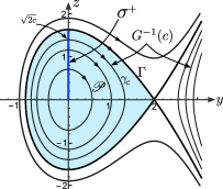
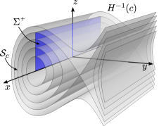
$a)$		$b)$

Figure 1. $a)$ Phase portrait of the planar Hamiltonian system associated with $G(y,z)$. $b)$ Foliation of the first integral of (16).

In the $yz-$plane, the intersection of the period annulus $\mathscr{P}$ with the positive $z$-axis is the line segment $\sigma^{+}:=\{(0,z)\;|\;0<z<\sqrt{8/3}\}$, which is a transversal section for the flow of the Hamiltonian system associated with $G(y,z)$. The dot product of the vector $(0,1,0)$, which is orthogonal to $\Sigma^{+}:=\mathbb{R}\times\sigma^{+}$, and the vector field $\mathcal{X}$, associated to (16), has defined sing: $\langle(0,1,0),\mathcal{X}\rangle=z>0$. Hence, $\Sigma^{+}$ is a $2$-dimensional transversal section for the flow of system (16).

As usual, we can use the energy level $c$ of $H$ to get the parametrization

$$\mathbb{R}\times(0,4/3)\longrightarrow\Sigma^{+},\,(x,c)\longmapsto(x,0,\sqrt{2c}),$$

of the transversal section $\Sigma^{+}.$ In other words, the points in $\Sigma^{+}$ can be described by the two coordinates $(x,c)$. Let $\phi_{\tau}(x,c)$ be the trajectory of system (16) passing through $(x,c)\in\Sigma^{+}$. Since the right-hand side of the system does not depend of $x$, $\phi_{\tau}(x,c)$ has the form $\big{(}x_{c}(\tau),\varphi_{\tau}(0,c)\big{)},$ where $\varphi_{\tau}(0,c)=(y_{c}(\tau),z_{c}(\tau))$ is the trajectory of the Hamiltonian system associated with $G(y,z)$, passing through the point $(0,c)\in\sigma^{+}$ at time $\tau=0$. Thus, there exists a well-defined Poincaré first return map

$$\begin{array}[]{rcl}\mathcal{P}\colon\Sigma^{+}&\longrightarrow&\Sigma^{+}\\ (x,c)&\longmapsto&\phi_{\tau(x,c)}(x,c),\end{array}$$

where $\tau(x,c)$ is the time of first return of the point $(x,c)$ to $\Sigma^{+}$.

Each trajectory $\phi_{\tau}(x,c)$ of the system starting in the region $\mathbb{R}\times\mathscr{P}\subset\mathbb{R}^{3}$ is contained in the surface $\mathcal{S}_{c}$ and $\Sigma^{+}\cap\mathcal{S}_{c}=\{(x,c)\;|\;x\in\mathbb{R}\}$, then the $c$-coordinate of $\mathcal{P}(x,c)$ remains invariant. Thus, $\mathcal{P}(x,c)=\phi_{\tau(x,c)}(x,c)=(x_{c}(\tau(x,c)),c)$, which implies that the fixed points of $\mathcal{P}$ are in correspondence with the zeros of the displacement function

$$L(x,c):=x_{c}(\tau(x,c))-x_{c}(0).$$

Since the right-hand side of the system (16) does not depend on $x$, the time of first return $\tau(x,c)$ does not either, that is, $\tau(x,c)=\tau(0,c)$. Thus, if $L(0,c^{*})=0$, then $L(x,c^{*})=0$ for all $x\in\mathbb{R}$, whence $\mathcal{S}_{c^{*}}$ will be a isochronous (periodic) surface, according to Definition 4.1. Hence, it is enough to study the function

$$L(0,c)=x_{c}(\tau(0,c))-x_{c}(0),\quad\mbox{with }x_{c}(0)=0.$$

To complete the proof, we will prove that $L(0,c)<0$ for $0<c\leq 2/3$, $L(0,c)>0$ for $2/3\ll c<4/3$, and $L(0,c)$ is a monotonous increasing function in $\big{(}2/3,4/3\big{)}$, which implies the existence of a unique $c^{*}\in(0,4/3)$ such that $L(0,c^{*})=0$. This will prove the uniqueness of the isochronous surface $\mathcal{S}_{c^{*}}$ . The proof of these assertions is analogous to the proof of the uniqueness of the limit cycle in the van der Pol differential system given in [10, Sec 12.3]. Hence, we will give the main ideas to prove the properties of $L(0,c)$ and we leave the details to the reader.

From the fundamental theorem of calculus and the first equation in (16) we have

$$L(0,c)=x_{c}(\tau(0,c))-x_{c}(0)=\int_{0}^{\tau(0,c)}x_{c}^{\prime}(\tau)\,d\tau=\int_{0}^{\tau(0,c)}(y_{c}(\tau)-1)\,d\tau.$$

In Figure 2 we show an sketch for the graph of $y_{c}(\tau)-1$, whose shape follows easily from $a)$ in Figure 1 and the fact that $G(1,0)=2/3$. Hence, for $0<c\leq 2/3$, $y_{c}(\tau)-1<0$ for almost all $\tau$, thus $L(0,c)<0$.

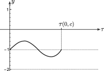
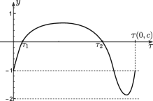
$a)$		$b)$

Figure 2. Graph of $y_{c}(\tau)-1$ for initial condition $(0,c)\in\Sigma^{+}$, with $c\in(0,2/3)$ in $a)$ and with $c$ close to $4/3$ in $b)$. The $\tau_{1}$ and $\tau_{2}$ are the positive times that $\varphi_{\tau}(0,c)$ needs to reach the vertical line $\{y=1\}$ by first and second time, respectively.

For $2/3<c<4/3,$ we rewrite the displacement function as

$$L(0,c)=\displaystyle\int_{\gamma_{c}}y-1.$$

Following [10, p.269], we divide the curve $\gamma_{c}$ into four curves $\gamma^{1}_{c},\gamma^{2}_{c},\gamma^{3}_{c},\gamma^{4}_{c}$ as shown in Figure 3. Let $y_{0}:=1-\sqrt{3}$ be the intersection of $\gamma_{2/3}$ with the negative $y-$axis.

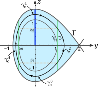
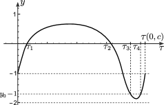
$a)$		$b)$

Figure 3. The curve $\gamma_{c}$ divided in the curves $\gamma_{c}^{1}$, $\gamma_{c}^{2}$, $\gamma_{c}^{3}$ and $\gamma_{c}^{4}$, with $2/3<c<4/3$, is showed in $a)$. The corresponding graph of $y_{c}(\tau)-1$ is showed in $b)$.

The curves $\gamma^{1}_{c}$ and $\gamma^{3}_{c}$ are defined for $y_{0}\leq y\leq 1,$ while the curves $\gamma^{2}_{c}$ and $\gamma^{2}_{c}$ are defined for $z_{1}\leq z\leq z_{2}$ (of course, $z_{1}$ and $z_{2}$ depend on $c$). Then

$$L(0,c)=L_{1}(c)+L_{2}(c)+L_{3}(c)+L_{4}(c),$$

where

$$L_{i}(c):=\displaystyle\int_{\gamma^{i}_{c}}y-1,\,\,i=1,2,3,4.$$

We can make an analogous analysis as in [10, p.270] to prove the following properties. $L_{1}(c)$ and $L_{3}(c)$ are negative monotonous increasing functions which are bounded in the interval $(2/3,4/3)$; $L_{2}(c)$ is a positive monotonous increasing function, which goes to infinity as $c$ goes to $4/3$; $L_{4}(c)$ is a negative decreasing function, which is bounded and whose derivative goes to zero as $c$ goes to $4/3.$ The properties on $L_{2}(c)$ and $L_{4}(c)$ imply that $L_{2}(c)+L_{4}(c)$ has a unique zero and $L_{2}(c)+L_{4}(c)$ goes to infinity as $c$ goes to $4/3.$ In addition, the properties on $L_{1}(c)$ and $L_{3}(c)$ imply that $L(0,c)$ has a unique zero $c^{*}$ in $(2/3,4/3).$ Furthermore, a more accurate analysis proves that $L(0,c)$ is a monotonous increasing function in $(2/3,4/3).$ ∎

Figure 4 shows part of the phase portrait of (16) close to the isochronous surface $\mathcal{S}_{c^{*}}$, where $c^{*}\in(1.6305,1.6310)$. More precisely, it gives part of the level surfaces of the first integral and the trajectories with initial conditions $(0,0,1.6323)$, in magenta, $(0,0,1.54919)$, in red, and $(0,0,1.6308)$, $(2.7,0,1.6308)$, $(-4,0,1.6308)$ in blue. The magenta trajectory advances in the positive direction of the $x$-axis, the red trajectory advances in the negative direction of the $x$-axis and the blue ones are (approximately) periodic, with the same period.

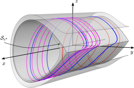
Figure 4. Existence of a isochronous surface $\mathcal{S}_{c^{*}}$ of system (16).

5. Concluding remarks

From the previous sections we can observe that the discrete and continuous dynamics of the nilpotent polynomial vector fields (1) share some similarities. For instance, from (8) it follows that the surface

$$w=\frac{a_{12}}{d_{2}p_{d_{2}}}u^{2}+A_{3}+\frac{a_{20}}{d_{2}p_{d_{2}}}$$

is reached from any initial point after one iteration. Thus, this surface contains the long-term dynamics of the system $(\mathbb{R}^{3},\mathbb{N}_{0},G)$, which is conjugated to (4). Similarly, since system (5) is polynomially integrable, its dynamics evolves in the algebraic level surfaces of the polynomial first integral. Hence, this reduction of the dynamics in one dimension is a similarity that, in general, share the discrete and continuous dynamical systems previously mentioned. Other similarity is that for the case $\deg A_{1}(x)=1$, the discrete dynamical system (4) and the continuous dynamical system (5) are completely understood. Indeed, from Theorem 1.1 the discrete system has a global attractor and from Theorem 1.2 the continuous system is polynomially completely integrable.

From conditions (3) we know that $\deg A_{1}(x)=1$ if $d_{2}>1$. Hence, according to the previous paragraph, the discrete and continuous dynamics of (1) will be more interesting for $d_{1}\geq 1$, $d_{2}=1$ and $\deg A_{1}(x)=2$.

The system (4) with $d_{2}=1$ has been studied in Statement 2) of Theorem 1.1. We have showed that in such case there exist a unique fixed point, there are not $2$-cycles and there exists at least one $3$-cycle. This triggers the following questions:

• How to discern analytically the existence of $m$-cycles with $m\geq 4$?

• Could be the $3$-cycle of Theorem 1.1 unique and attractor?

The system (5), with $d_{1}=d_{2}=1$ have been analyzed in Proposition 1.3. We showed that when the associated planar Hamiltonian system has only one period annulus, the system has only one isochronous periodic surface $\mathcal{S}_{\mu}$. Concerning this result a natural question arise:

• Is any periodic orbit in $\mathcal{S}_{\mu}$ persisting under the perturbation $\lambda I$ with $\lambda<0$?

A positive answer to the this question would give a affirmative response to the Problem 19 in [9], which is related with the Markus–Yamabe Conjecture.

We note that for $d_{1}>1$ the planar Hamiltonian system associated with system (5) can have several period annuli. For instance, by taking $P_{1}(s)=s^{2}-s-3$, $P_{2}(s)=s$, $a_{12}=1$ and $A_{3}=-6$, the system (5) has two period annuli. Hence, we can ask:

• How many periodic surfaces can have system (5) for $d_{1}\geq 1$ and $d_{2}=1$?

This question is in some sense analogous to the problem about the number of limit cycles in planar polynomial vector fields. See [11, 15] and references there in.

In this work, we have focused in the discrete and continuous dynamics of the nilpotent polynomial vector fields in dimension three. However, we believe that the techniques used in the present research are useful also for an analogous study in higher dimensions. Recall that in [2] is provided the characterization of a wide class of nilpotent polynomial vector fields in any dimension. Of course, the generalization or extension of the results presented here is no simple. For example, in dimension four there are six different families of nilpotent polynomial vector fields to be analyzed. We expect that in some of these families could be arise different behaviors than those obtained here.

References

- [1] H. Bass, E. Connell, D. Wright, The Jacobian conjecture: reduction of degree and formal expansion of the inverse, Bull. Am. Math. Soc. 2 (1982) 287–330.
- [2] Á. Castañeda, A. van den Essen, A new class of nilpotent Jacobians in any dimension, J. Algebra 566 (2021), 283–301.
- [3] M. Chamberland, Dynamics of maps with nilpotent Jacobians, J. Difference. Equ. Appl. 12 (2006), 49–56.
- [4] M. Chamberland, A. van den Essen, Nilpotent Jacobians in dimension three, Journal of Pure and Applied Algebra, 205 (2006), 146–155.
- [5] A. Cima, A. van den Essen, A. Gasull, E. Hubbers and F. Mañosas, A polynomial counterexample to the Markus–Yamabe conjecture, Adv. Math. 131 (1997), 453–457.
- [6] A. Cima, A. Gasull, F. Mañosas, The discrete Markus-Yamabe problem, Nonlinear Anal. 35 (1999), 343–354.
- [7] A. van den Essen, Polynomial Automorphisms and the Jacobian Conjecture, Progress in Mathematics, vol. 190, Birkhäuser, Basel, 2000.
- [8] A. van den Essen, S. Kuroda, A.J. Crachiola, Polynomial Automorphisms and the Jacobian Conjecture New Results from the Beginning of the 21st century, Frontiers in Mathematics, (2021), Birkhäuser.
- [9] A. Gasull, Some open problems in low dimensional dynamical systems, SeMA Journal 78 (2021), 233–269.
- [10] M.W. Hirsch, S. Smale, R.L. Devaney, Differential Equations, Dynamical Systems, and an Introduction to Chaos, Elsevier/Academic Press, Amsterdam, 2013.
- [11] Y. Ilyashenko, Centennial history of Hilbert’s 16th problem, Bull. Amer. Math. Soc. (N.S.) 39 (2002), 301–354.
- [12] Y.A. Kuznetsov, Elements of Applied Bifurcation Theory, Applied Mathematical Sciences 112, Springer, 2004.
- [13] J.P. La Salle, The stability of dynamical systems, CBMS-NSF Regional Conference Series in Applied Math. Vol. 25, 1976.
- [14] L. Markus, H. Yamabe, Global stability criteria for differential systems, Osaka Math. J. 12 (1960), 305–317.
- [15] S. Rebollo-Perdomo, The infinitesimal Hilbert’s 16th problem in the real and complex planes, Qual. Theory Dyn. Syst. 7 (2009), 467–500.
- [16] A.V. Yagzhev, On Keller’s problem, Sib. Math. J. 21 (1980), 747–754.
- [17] D. Yan. M. de Bondt, The classification of some polynomial maps with nilpotent Jacobians. Linear Algebra Appl. 565 (2019), 287–308.
- [18] D. Yan, G. Tang, Polynomial maps with nilpotent Jacobians in dimension three, Linear Algebra Appl. 489 (2016), 298–323.