100
Reduced models with nonlinear approximations of latent dynamics for model premixed flame problems††thanks: This work was supported in part by the Air Force Center of Excellence on Multi-Fidelity Modeling of Rocket Combustor Dynamics, award FA9550-17-1-0195. The fourth author was additionally partially supported by NSF-2012250 and by the Air Force Office of Scientific Research (AFOSR) award FA9550-21-1-0222 (Dr. Fariba Fahroo).
Abstract
Efficiently reducing models of chemically reacting flows is often challenging because their characteristic features such as sharp gradients in the flow fields and couplings over various time and length scales lead to dynamics that evolve in high-dimensional spaces. In this work, we show that online adaptive reduced models that construct nonlinear approximations by adapting low-dimensional subspaces over time can predict well latent dynamics with properties similar to those found in chemically reacting flows. The adaptation of the subspaces is driven by the online adaptive empirical interpolation method, which takes sparse residual evaluations of the full model to compute low-rank basis updates of the subspaces. Numerical experiments with a premixed flame model problem show that reduced models based on online adaptive empirical interpolation accurately predict flame dynamics far outside of the training regime and in regimes where traditional static reduced models, which keep reduced spaces fixed over time and so provide only linear approximations of latent dynamics, fail to make meaningful predictions.
keywords:
model reduction Kolmogorov barrier transport-dominated problems chemically reacting flows empirical interpolation1 Introduction
Even with advances in modern computational capabilities, high-fidelity, full-scale simulations of chemically reacting flows in realistic applications remain computationally expensive [19, 29, 18, 20]. Traditional model reduction methods [42, 4, 1, 38] that seek reduced solutions in low-dimensional subspaces fail for problems that involve chemically reacting advection-dominated flows because the strong advection of sharp gradients in the solution fields lead to high-dimensional features in the latent dynamics; see [39] for an overview of the challenges of model reduction of strongly advecting flows and other problems with high-dimensional latent dynamics. We demonstrate on a model premixed flame problem [46]—which greatly simplifies the reaction and flow dynamics but preserves some of the model reduction challenges of more realistic chemically reacting flows—that adapting subspaces of reduced models over time [37, 35, 9] can help to provide accurate future-state predictions with only a few degrees of freedom.
Traditional reduced models are formulated via projection-based approaches that seek approximate solutions in lower dimensional subspaces of the high-dimensional solution spaces of full models; see [42, 4, 1] for surveys on model reduction. Mathematically, the traditional approximations in subspaces lead to linear approximations in the sense that the parameters of the reduced models that can be changed over time enter linearly in the reduced solutions. It has been observed empirically that for certain types of dynamics, which are found in a wide range of science and engineering applications, including chemically reacting flows, the accuracy of such linear approximations grows slowly with the dimension of the reduced space. Examples of such dynamics are flows that are dominated by advection. In fact, for solutions of the linear advection equation, it has been shown that under certain assumptions on the metric and the ambient space the best-approximation error of linear approximations in subspaces cannot decay faster than . This slowly decaying lower bound is referred to as the Kolmogorov barrier, because the Kolmogorov -width of a set of functions is defined as the best-approximation error obtained over all subspaces; see [32, 14, 8] for details.
A wide range of methods has been introduced that aim to circumvent the Kolmogorov barrier; see [39] for a brief survey. There are methods that introduce nonlinear transformations and nonlinear embeddings to recover low-dimensional structures. Examples are transformations based on Wasserstein metrics [12], deep network and deep autoencoders [24, 21, 41, 5], shifted proper orthogonal decomposition and its extensions [40, 34], quadratic manifolds [13, 2], and other transformations [31, 44, 30, 6]. In this work, we focus on online adaptive reduced models that adapt the reduced space over time to achieve nonlinear approximations. In particular, we build on online adaptive empirical interpolation with adaptive sampling (AADEIM), which adapts reduced spaces with additive low-rank updates that are derived from sparse samples of the full-model residual [37, 35, 9]. The AADEIM method builds on empirical interpolation [3, 7, 11]. We refer to [43, 22, 48, 23, 27, 28, 16] for other adaptive basis and adaptive low-rank approximations. The idea of evolving basis functions over time has a long history in numerical analysis and scientific computing, which dates back to at least Dirac [10].
We apply AADEIM to construct reduced models of a model premixed flame problem with artificial pressure forcing. Our numerical results demonstrate that reduced models obtained with AADEIM provide accurate predictions of the fluid flow and flame dynamics with only a few degrees of freedom. In particular, the AADEIM model that we derive predicts the dynamics far outside of the training regime and in regimes where traditional, static reduced models, which keep the reduced spaces fixed over time, fail to provide meaningful prediction.
The manuscript is organized as follows. We first provide preliminaries in Section 2 on traditional, static reduced modeling. We then recap AADEIM in Section 3 and highlight a few modifications that we made compared to the original AADEIM method introduced in [37, 35]. The reacting flow solver PERFORM [46] and the model premixed flame problem is discussed in Section 4. Numerical results that demonstrate AADEIM on the premixed flame problem are shown in Section 5 and conclusions are drawn in Section 6.
2 Static model reduction with empirical interpolation
We briefly recap model reduction with empirical interpolation [3, 15, 7, 11] using reduced spaces that are fixed over time. We refer to reduced models with fixed reduced spaces as static models in the following sections.
2.1 Static reduced models
Discretizing a system of partial differential equations in space and time can lead to a dynamical system of the form
| (1) |
with state at time step and physical parameter . The function is vector-valued and nonlinear in the first argument in the following. A system of form (1) is obtained, for example, after an implicit time discretization of the time-continuous system. The initial condition is and is an element of the set of initial conditions .
Consider now training parameters with training initial conditions . Let further be the corresponding training trajectories defined as
From the snapshot matrix , a reduced space of dimension with basis matrix is constructed, for example, via proper orthogonal decomposition (POD) or greedy methods [42, 4].
The static Galerkin reduced model is
with the initial condition for a parameter and reduced state at time . However, evaluating the function still requires evaluating at all components. Empirical interpolation [3, 15, 7, 11] provides an approximation of that can be evaluated at a vector with costs that grow as . Consider the matrix that has as columns the -dimensional unit vectors with ones at unique components . It holds for the number of points . The points can be computed, for example, with greedy [3, 7], QDEIM [11], or oversampling algorithms [36, 47]. We denote with that only the component functions corresponding to the points of the vector-valued function are evaluated at and . The empirical-interpolation approximation of is
where denotes the Moore–Penrose inverse (pseudoinverse) of .
Based on the empirical-interpolation approximation , we derive the static reduced model
with the reduced states at time steps .
2.2 The Kolmogorov barrier of static reduced models
The empirical-interpolation approximation depends on the basis matrix , which is fixed over all time steps . This means that the reduced approximation at time depends linearly on the basis vectors of the reduced space , which are the columns of the basis matrix . Thus, the lowest error that such a static reduced model can achieve is related to the Kolmogorov -width, i.e., the best-approximation error in any subspace of dimension . We refer to [39] for an overview of the Kolmogorov barrier in model reduction and to [8, 26, 32] for in-depth details. It has been observed empirically, and in some limited cases proven, that systems that are governed by dynamics with strong advection and transport exhibit a slowly decaying -width, which means that linear, static reduced models are inefficient in providing accurate predictions.
3 Online adaptive empirical interpolation methods for nonlinear model reduction
In this work, we apply online adaptive model reduction methods to problems motivated by chemically reacting flows, which are often dominated by advection and complex transport dynamics that make traditional static reduced models inefficient. We focus on reduced models obtained with AADEIM, which builds on the online adaptive empirical interpolation method [37] for adapting the basis and on the adaptive sampling scheme introduced in [35, 9]. We utilize the one-dimensional compressible reacting flow solver PERFORM [46], which provides several benchmark problems motivated by combustion applications. We will consider a model premixed flame problem with artificial pressure forcing and show that AADEIM provides reduced models that can accurately predict the flame dynamics over time, whereas traditional static reduced models fail to make meaningful predictions.
For ease of exposition, we drop the dependence of the states on the parameter in this section.
3.1 Adapting the basis
To allow adapting the reduced space over time, we formally make the basis matrix and the points matrix with points depend on the time step . In AADEIM, the basis matrix is adapted at time step to the basis matrix via a rank-one update
given by and . To compute an update at time step , we introduce the data matrix , where is a window size. First, similarly the empirical-interpolation points, we consider sampling points and the corresponding sampling matrix . We additionally consider the complement set of sampling points and the corresponding matrix . We will also need the matrix corresponding to the union of the set of sampling points and the points , which we denote with , and its complement .
The data matrix at time step is then given by
where we add the vector that is defined as
| (2) |
The state used in (2) is the reduced state at time step . The vector at time step serves as an approximation of the full-model state at time . This is motivated by the full-model equations (1) with the reduced state as an approximation of the full-model state at time step ; we refer to [35] for details about this motivation.
The AADEIM basis update at time step is the solution to the minimization problem
| (3) |
where the coefficient matrix is
| (4) |
The matrix is adapted to by applying QDEIM [11] to the adapted basis matrix
We make two modifications compared to the original AADEIM approach. First, we sample from the points given by , which is the union of the sampling points and the points . This comes with no extra costs because the full-model right-hand side function needs to be evaluated at the points corresponding to and even in the original AADEIM approach. Second, as proposed in [17], we adapt the basis at all components of the residual in the objective, rather than only at the sampling points given by . This requires no additional full-model right-hand side function evaluations but comes with increased computational costs when solving the optimization problem (3). However, typically solving the optimization problem is negligible compared to sparsely evaluating the full-model right-hand side function.
3.2 Adapting sampling points
When adapting the sampling matrix to at time step , we evaluate the full-model right-hand side function at all components to obtain
| (5) |
and put it as column into the data matrix . We then compute the residual matrix
Let denote the 2-norm of the -th row of and let be an ordering such that
At time step , we pick the first indices as the sampling points to form , which is subsequently used to adapt the basis matrix from to .
Two remarks are in order. First, the sampling points are quasi-optimal with respect to an upper bound of the adaptation error [9]. Second, adapting the sampling points requires evaluating the residual at all components, which incurs computational costs that scale with the dimension of the full-model states. However, we adapt the sampling points not every time step, but only every -th time step as proposed in [35].
3.3 Computational procedure and costs
By combining the basis adaptation described in Section 3.1 and sampling-points adaptation of Section 3.2, we obtain the AADEIM reduced model
where now the approximation is
which depends on the time step because the basis and the points matrix depend on the time step. The AADEIM algorithm is summarized in Algorithm 1. Inputs to the algorithm are the initial condition , full-model right-hand side function , parameter , reduced dimension , initial window size , window size , and the frequency of updating the sampling points . The algorithm returns the trajectory .
Lines 2–6 initialize the AADEIM reduced model by first solving the full model for time steps to compute the snapshots and store them in the columns of the matrix . From these snapshots, a POD basis matrix for time step is constructed. The time-integration loop starts in line 7. In each iteration , the reduced state is propagated forward to obtain by solving the AADEIM reduced model for one time step. The first branch of the if clause in line 10 is entered if the sampling points are to be updated, which is the case every -th time step. If the sampling points are updated, the full-model right-hand side function is evaluated at all components to compute the residual matrix . The new sampling points are selected based on the largest norm of the rows of the entry-wise squared residual matrix . If the sampling points are not updated, the full-model right-hand side function is evaluated only at the points corresponding to and . All other components are approximated with empirical interpolation. In lines 21 and 22, the basis update is computed and then used to obtain the adapted basis matrix . The points are adapted to by applying QDEIM to the adapted basis matrix in line 23. The method solveFOM() refers to the full-model solver and the method qdeim() to QDEIM [11]
4 Benchmarks of chemically reacting flow problems
A collection of benchmarks for model reduction of transport-dominated problems is provided with PERFORM [46]. Documentation of the code and benchmark problems is available online444https://perform.readthedocs.io/. The benchmarks are motivated by combustion processes and modeled after the General Equations and Mesh Solver (GEMS), which provides a reacting flow solver in three spatial dimensions [25].
|
|
 |
 |
| (a) pressure, | (b) pressure, | (c) pressure, |
 |
 |
 |
| (d) velocity, | (e) velocity, | (f) velocity, |
 |
 |
 |
| (g) temperature, | (h) temperature, | (i) temperature, |
 |
 |
 |
| (j) mass fraction, | (k) mass fraction, | (l) mass fraction, |
4.1 Numerical solver description
PERFORM numerically solves the one-dimensional Navier-Stokes equations with chemical species transport and a chemical reaction source term:
with
| (6) |
where is the conserved state at time and spatial coordinate , is the inviscid flux vector, is the viscous flux vector, and is the source term. Additionally, is density, is velocity, is stagnation enthalpy, is static pressure, and is mass fraction of the th chemical species. The reaction source corresponds to the reaction model, which is described by an irreversible Arrhenius rate equation. The problem is discretized in the spatial domain with a second-order accurate finite volume scheme. The inviscid flux is computed by the Roe scheme [33]. Gradients are limited by the Venkatakrishnan limiter [45]. The time derivative is discretized with the first-order backwards differentiation formula scheme (i.e. backward Euler). Calculation of the viscous stress , heat flux , and diffusion velocity , and any additional details about the implementation can be found in PERFORM’s online documentation.
4.2 Premixed flame with artificial forcing
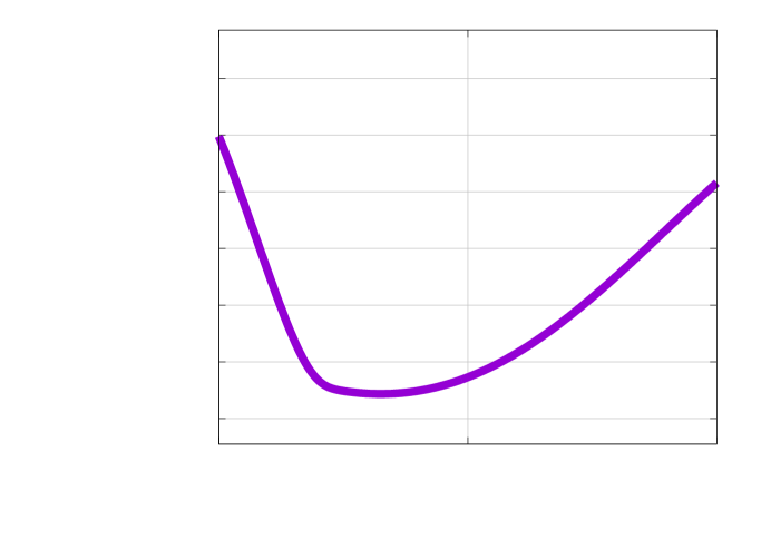
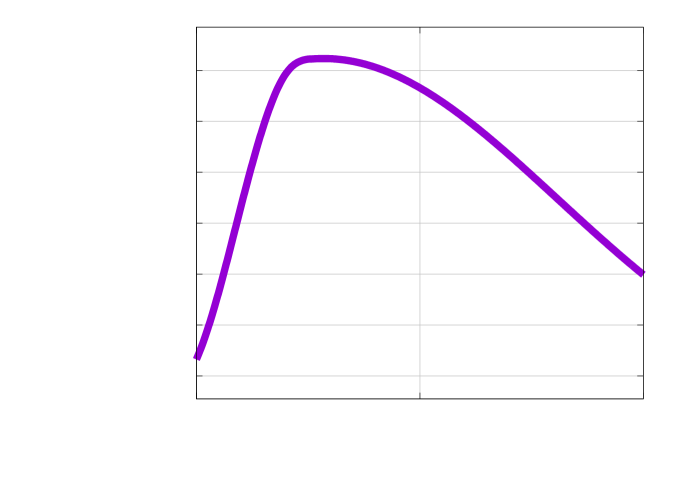
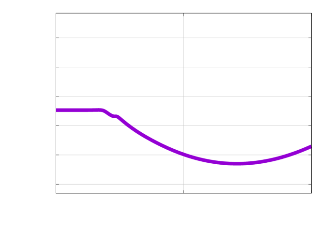
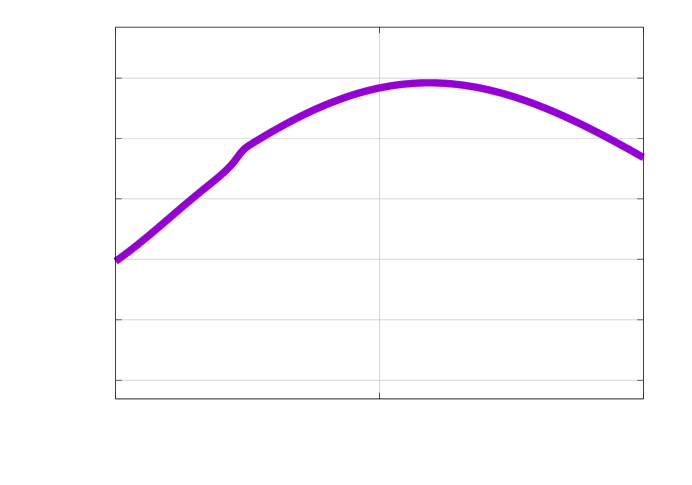
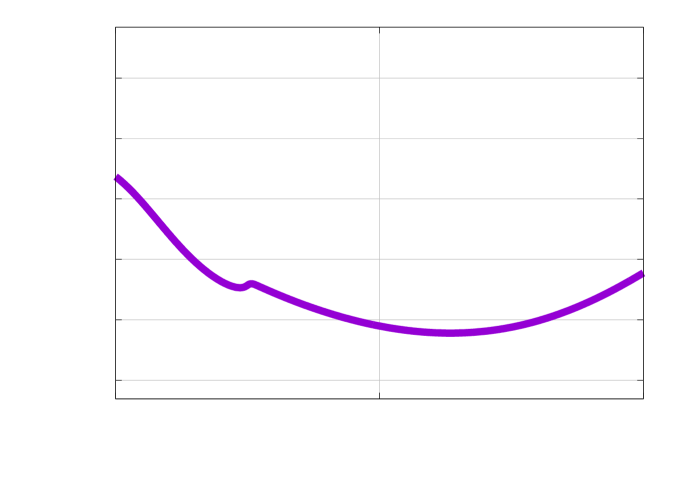
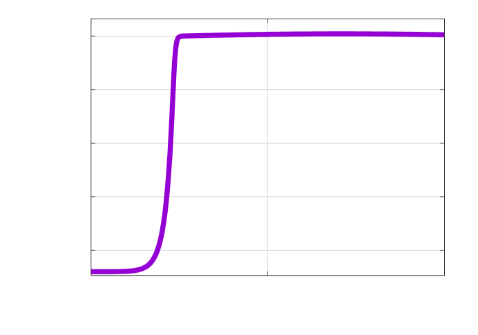
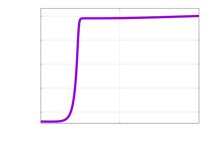
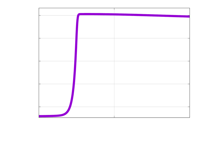
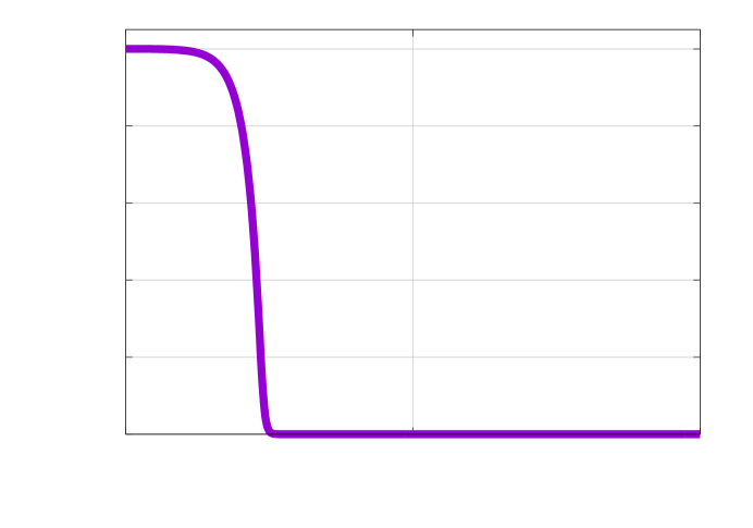
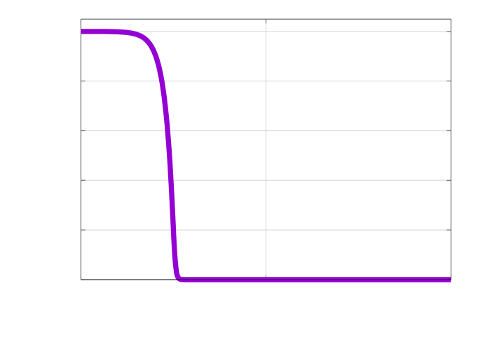
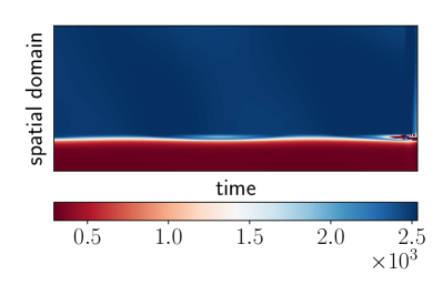
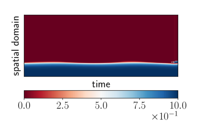
We consider a setup corresponding to a model premixed flame with artificial pressure forcing. There are two chemical species: “reactant” and “product”. The reaction is a single-step irreversible mechanism that converts low-temperature reactant to high-temperature product, modeling a premixed combustion process. An artificial sinusoidal pressure forcing is applied at the outlet, which causes an acoustic wave to propagate upstream. The interaction between different length and time scales given by the system acoustics caused by the forcing and the flame leads to strongly nonlinear system dynamics with multiscale effects. The result are dynamics that evolve in high-dimensional spaces and thus are inefficient to reduce with static reduced models; see Section 2.2. The states of the full model and how they evolve over time are shown in Figure 1.
5 Numerical results
We demonstrate nonlinear model reduction with online adaptive empirical interpolation on the model premixed flame problem introduced in Section 4.2.
 |
 |
| (a) pressure | (b) velocity |
 |
 |
| (c) temperature | (d) species mass fraction |
 |
 |
| (a) global in time | (b) local in time |
5.1 Numerical setup of full model
Consider the problem described in Section 4.2. Each of the four conserved quantities , , , is discretized on equidistant grid points in the domain m, which leads to a total of unknowns of the full model. The time-step size is s and the end time is s, which is a total of time steps. A 10% sinusoidal pressure perturbation at a frequency of 50 kHz is applied at the outlet.
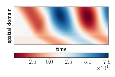
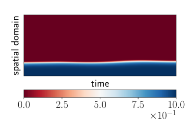
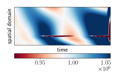
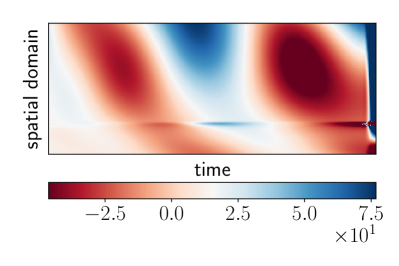
Space-time plots of pressure, velocity, temperature, and species mass fraction are shown in Figure 2. Pressure and velocity shown in plots (a) and (b) of Figure 2 show a transport-dominated behavior, which is in agreement with the pressure and velocity waves shown in Figure 1.
 |
 |
| (a) pressure | (b) velocity |
 |
 |
| (c) temperature | (d) species mass fraction |
5.2 Static reduced models
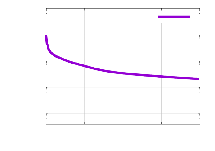
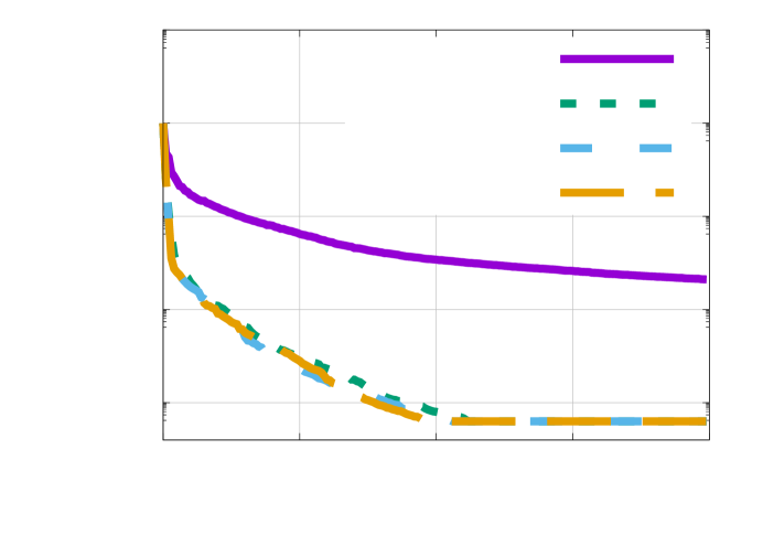
Snapshots are generated with the full model by querying (1) for 35,000 time steps and storing the full model state every 50 time steps. The singular values of the snapshot matrix are shown in Figure 3a, which decay slowly and indicate that static reduced models are inefficient. From the snapshots, we generate POD bases of dimension and to derive reduced models with empirical interpolation. The interpolation points are selected with QDEIM [11]. The empirical interpolation points are computed separately with QDEIM for each of the four variables in (6). Then, we select a component of the state as an empirical interpolation point if it is selected for at least one variable.
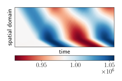
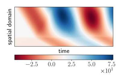
The time-space plots of the static reduced approximation of the full-model dynamics are shown in Figure 4 for dimension . The approximation is poor, which is in agreement with the transport-dominated dynamics and the slow decay of the singular values shown in Figure 3a. The time-space plot of the static reduced model of dimension gives comparably poor approximations and is not shown here. It is important to note that the static reduced model is derived from snapshots over the whole time range from to end time , which means that the static reduced model has to merely reconstruct the dynamics that were seen during training, rather than predicting unseen dynamics. This is in stark contrast to the adaptive reduced model derived with AADEIM in the following subsection, where the reduced model will predict states far outside of the training window.
 |
 |
| (a) pressure | (b) velocity |
 |
 |
| (c) temperature | (d) species mass fraction |
5.3 Reduced model with AADEIM
We derive a reduced model with AADEIM of dimension . The initial window size is and the window size is , as recommended in [35]. Notice that an initial window means that the AADEIM model predicts unseen dynamics (outside of training data) starting at time step , which corresponds to . This is in stark contrast to Section 5.2 where the static reduced model only has to reconstruct seen dynamics. The number of sampling points is and the frequency of adapting the sampling points is . This means that the sampling points are adapted every third time step; see Algorithm 1. The basis matrix and the points matrix are adapted every other time step.
 |
 |
| (a) error | (b) costs |
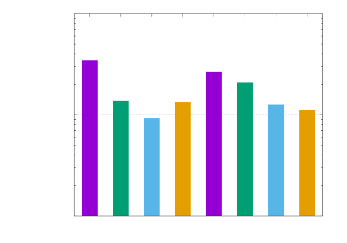
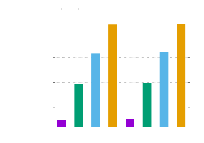
A: dimension , update frequency , #sampling points B: dimension , update frequency , #sampling points C: dimension , update frequency , #sampling points D: dimension , update frequency , #sampling points E: dimension , update frequency , #sampling points F: dimension , update frequency , #sampling points G: dimension , update frequency , #sampling points H: dimension , update frequency , #sampling points
 |
 |
| (a) dimension | (b) dimension |
The time-space plot of the prediction made with the AADEIM model is shown in Figure 5. The predicted states obtained with the AADEIM model are in close agreement with the full model (Figure 2), in contrast to the states derived with the static reduced model (Figure 4). This also in agreement with the fast decay of the singular values of snapshots in local time windows, as shown in Figure 3b.
We further consider AADEIM models with dimension , initial window , and sampling points and frequency of adapting the sampling points . We compute the average relative error as
| (7) |
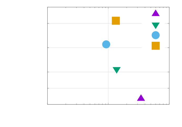
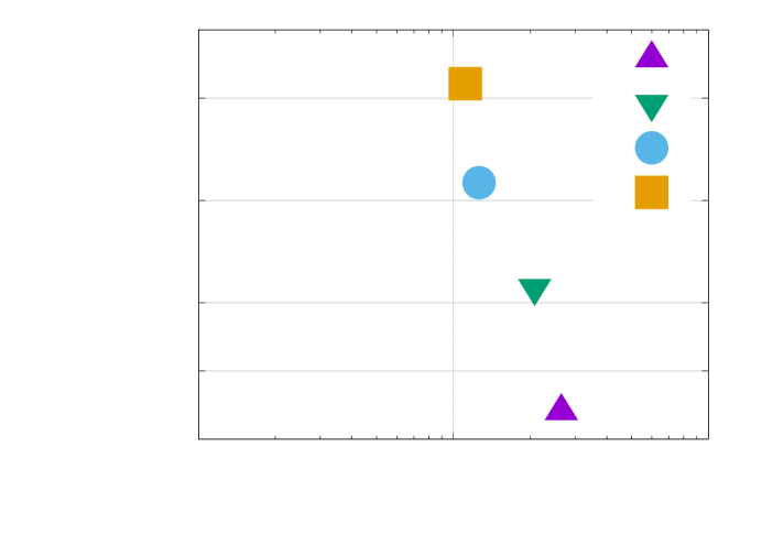
where is the trajectory obtained with the full model and is the reduced trajectory obtained with AADEIM from Algorithm 1. All combinations of models and their performance in terms of average relative error are shown in Figure 6a. As costs, we count the number of components of the full-model right-hand side function that need to be evaluated and report them in Figure 6b; see also Figure 7. All online adaptive reduced models achieve a comparable error of , where a higher number of sampling points and a more frequent adaptation of the sampling points typically leads to lower errors in favor of higher costs. These numerical observations are in agreement with the principles of AADEIM and the results shown in [37, 35, 9].
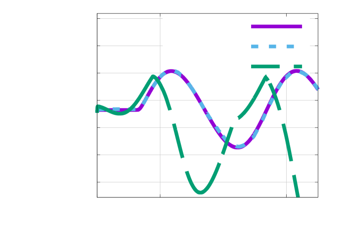
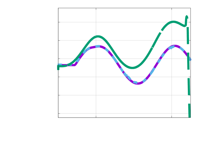
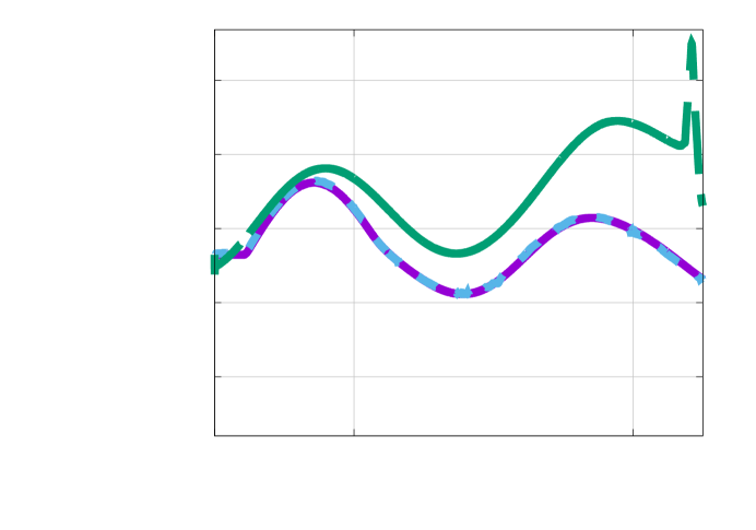
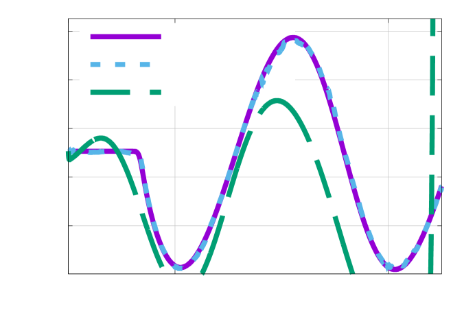
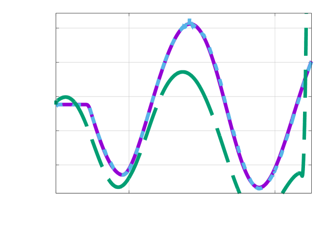
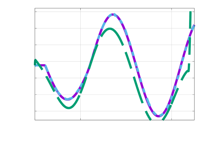
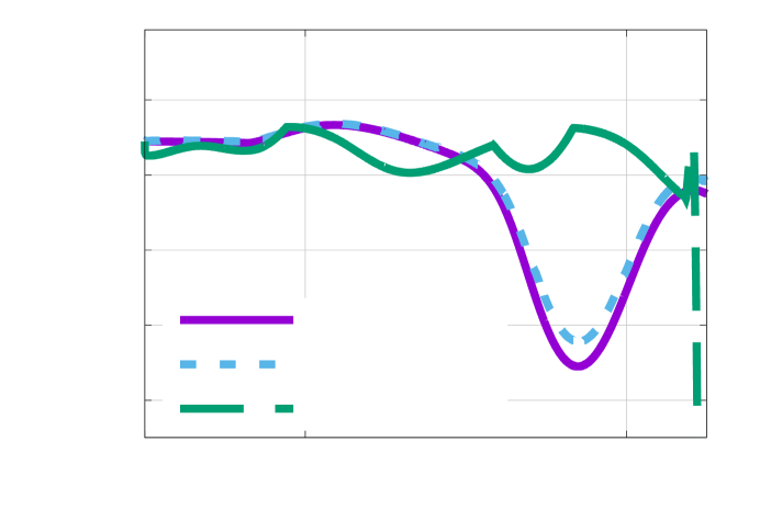
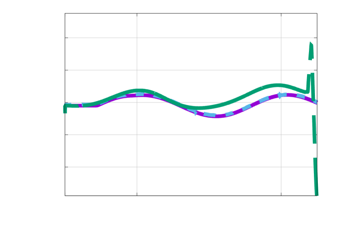
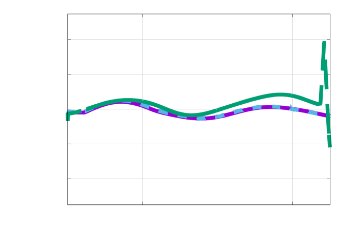
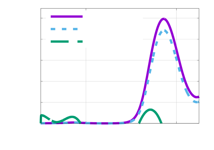
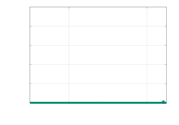
We now compare the AADEIM and static reduced model based on probes of the states at , , and . The probes for dimension , update frequency of the samples, and number of sampling points is shown in Figure 8. The probes obtained with the static reduced model of dimension and the full model are plotted too. The AADEIM model provides an accurate predictions of the full model over all times and probe locations for all quantities, whereas the static reduced model fails to provide meaningful approximations. Note that the mass fraction at probe location 2 and 3 is zero.
 |
 |
 |
| (a) pressure, probe 1 | (b) pressure, probe 2 | (c) pressure, probe 3 |
 |
 |
 |
| (d) velocity, probe 1 | (e) velocity, probe 2 | (f) velocity, probe 3 |
 |
 |
 |
| (g) temperature, probe 1 | (h) temperature, probe 2 | (i) temperature, probe 3 |
 |
 |
 |
| (j) mass fraction, probe 1 | (k) mass fraction, probe 2 | (l) mass fraction, probe 3 |
6 Conclusions
The considered benchmark problem of a model premixed flame with artificial pressure forcing relies on strong simplifications of physics that are present in more realistic scenarios of chemically reacting flows. However, it preserves the transport-dominated and multiscale nature of the dynamics, which are major challenges for model reduction with linear approximations. We showed numerically that online adaptive model reduction with the AADEIM method provides accurate predictions of the flame dynamics with few degrees of freedom. The AADEIM method leverages two properties of the considered problem. First, the states of the considered problem have a local low-rank structure in the sense that the singular values decay quickly for snapshots in a local time window. Second, the residual of the AADEIM approximation is local in the spatial domain, which means that few sampling points are sufficient to inform the adaptation of the reduced basis. Reduced models based on AADEIM build on these two properties to derive nonlinear approximations of latent dynamics and so enable predictions of transport-dominated dynamics far outside of training regimes.
References
- [1] Antoulas, A.C., Beattie, C.A., Gugercin, S.: Interpolatory Methods for Model Reduction. SIAM (2020)
- [2] Barnett, J., Farhat, C.: Quadratic approximation manifold for mitigating the Kolmogorov barrier in nonlinear projection-based model order reduction. Journal of Computational Physics 464, 111348 (2022)
- [3] Barrault, M., Maday, Y., Nguyen, N.C., Patera, A.: An ‘empirical interpolation’ method: application to efficient reduced-basis discretization of partial differential equations. Comptes Rendus Mathematique 339(9), 667–672 (2004)
- [4] Benner, P., Gugercin, S., Willcox, K.: A survey of projection-based model reduction methods for parametric dynamical systems. SIAM Review 57(4), 483–531 (2015)
- [5] Bruna, J., Peherstorfer, B., Vanden-Eijnden, E.: Neural Galerkin scheme with active learning for high-dimensional evolution equations. arXiv 2203.01360 (2022)
- [6] Cagniart, N., Maday, Y., Stamm, B.: Model order reduction for problems with large convection effects. In: Chetverushkin, B.N., Fitzgibbon, W., Kuznetsov, Y., Neittaanmäki, P., Periaux, J., Pironneau, O. (eds.) Contributions to Partial Differential Equations and Applications. pp. 131–150. Springer International Publishing, Cham (2019)
- [7] Chaturantabut, S., Sorensen, D.: Nonlinear model reduction via discrete empirical interpolation. SIAM Journal on Scientific Computing 32(5), 2737–2764 (2010)
- [8] Cohen, A., DeVore, R.: Kolmogorov widths under holomorphic mappings. IMA J. Numer. Anal. 36(1), 1–12 (2016)
- [9] Cortinovis, A., Kressner, D., Massei, S., Peherstorfer, B.: Quasi-optimal sampling to learn basis updates for online adaptive model reduction with adaptive empirical interpolation. In: American Control Conference (ACC) 2020. IEEE (2020)
- [10] Dirac, P.A.M.: Note on exchange phenomena in the Thomas Atom. Mathematical Proceedings of the Cambridge Philosophical Society 26(3), 376–385 (1930)
- [11] Drmač, Z., Gugercin, S.: A new selection operator for the discrete empirical interpolation method—improved a priori error bound and extensions. SIAM Journal on Scientific Computing 38(2), A631–A648 (2016)
- [12] Ehrlacher, V., Lombardi, D., Mula, O., Vialard, F.X.: Nonlinear model reduction on metric spaces. Application to one-dimensional conservative PDEs in Wasserstein spaces. ESAIM Math. Model. Numer. Anal. 54(6), 2159–2197 (2020)
- [13] Geelen, R., Wright, S., Willcox, K.: Operator inference for non-intrusive model reduction with nonlinear manifolds. arXiv 2205.02304 (2022)
- [14] Greif, C., Urban, K.: Decay of the Kolmogorov -width for wave problems. Appl. Math. Lett. 96, 216–222 (2019)
- [15] Grepl, M.A., Maday, Y., Nguyen, N.C., Patera, A.T.: Efficient reduced-basis treatment of nonaffine and nonlinear partial differential equations. ESAIM: Mathematical Modelling and Numerical Analysis 41(03), 575–605 (2007)
- [16] Hesthaven, Jan S., Pagliantini, Cecilia, Ripamonti, Nicolò: Rank-adaptive structure-preserving model order reduction of hamiltonian systems. ESAIM: M2AN 56(2), 617–650 (2022)
- [17] Huang, C., Duraisamy, K.: Predictive reduced order modeling of chaotic multi-scale problems using adaptively sampled projections (2022), in preparation
- [18] Huang, C., Duraisamy, K., Merkle, C.: Challenges in reduced order modeling of reacting flows. In: 2018 Joint Propulsion Conference (2018)
- [19] Huang, C., Wentland, C.R., Duraisamy, K., Merkle, C.: Model reduction for multi-scale transport problems using model-form preserving least-squares projections with variable transformation. J. Comp. Phys. 448, 110742 (2022)
- [20] Huang, C., Xu, J., Duraisamy, K., Merkle, C.: Exploration of reduced-order models for rocket combustion applications. In: 2018 AIAA Aerospace Sciences Meeting (2018)
- [21] Kim, Y., Choi, Y., Widemann, D., Zohdi, T.: A fast and accurate physics-informed neural network reduced order model with shallow masked autoencoder. Journal of Computational Physics 451, 110841 (2022)
- [22] Koch, O., Lubich, C.: Dynamical low‐rank approximation. SIAM Journal on Matrix Analysis and Applications 29(2), 434–454 (2007)
- [23] Kramer, B., Peherstorfer, B., Willcox, K.: Feedback control for systems with uncertain parameters using online-adaptive reduced models. SIAM Journal on Applied Dynamical Systems 16(3), 1563–1586 (2017)
- [24] Lee, K., Carlberg, K.T.: Model reduction of dynamical systems on nonlinear manifolds using deep convolutional autoencoders. J. Comput. Phys. 404, 108973, 32 (2020)
- [25] Li, D., Xia, G., Sankaran, V., Merkle, C.L.: Computational framework for complex fluid physics applications. In: Groth, C., Zingg, D.W. (eds.) Computational Fluid Dynamics 2004. pp. 619–624. Springer Berlin Heidelberg, Berlin, Heidelberg (2006)
- [26] Maday, Y., Patera, A.T., Turinici, G.: Global a priori convergence theory for reduced-basis approximations of single-parameter symmetric coercive elliptic partial differential equations. C. R. Math. Acad. Sci. Paris 335(3), 289–294 (2002)
- [27] Musharbash, E., Nobile, F., Zhou, T.: Error analysis of the dynamically orthogonal approximation of time dependent random PDEs. SIAM Journal on Scientific Computing 37(2), A776–A810 (2015)
- [28] Musharbash, E., Nobile, F., Vidličková, E.: Symplectic dynamical low rank approximation of wave equations with random parameters. BIT Numerical Mathematics 60(4), 1153–1201 (Dec 2020)
- [29] Nguyen, V., Buffoni, M., Willcox, K., Khoo, B.: Model reduction for reacting flow applications. International Journal of Computational Fluid Dynamics 28(3-4), 91–105 (2014)
- [30] Nonino, M., Ballarin, F., Rozza, G., Maday, Y.: Overcoming slowly decaying Kolmogorov n-width by transport maps: application to model order reduction of fluid dynamics and fluid–structure interaction problems. arXiv 1911.06598 (2019)
- [31] Ohlberger, M., Rave, S.: Nonlinear reduced basis approximation of parameterized evolution equations via the method of freezing. C. R. Math. Acad. Sci. Paris 351(23-24), 901–906 (2013)
- [32] Ohlberger, M., Rave, S.: Reduced basis methods: Success, limitations and future challenges. Proceedings of the Conference Algoritmy pp. 1–12 (2016)
- [33] P. L. Roe: Approximate Riemann solvers, parameter vectors, and difference schemes. Journal of Computational Physics 43, 357–372 (1981)
- [34] Papapicco, D., Demo, N., Girfoglio, M., Stabile, G., Rozza, G.: The neural network shifted-proper orthogonal decomposition: A machine learning approach for non-linear reduction of hyperbolic equations. Computer Methods in Applied Mechanics and Engineering 392, 114687 (2022)
- [35] Peherstorfer, B.: Model reduction for transport-dominated problems via online adaptive bases and adaptive sampling. SIAM Journal on Scientific Computing 42, A2803–A2836 (2020)
- [36] Peherstorfer, B., Drmac, Z., Gugercin, S.: Stability of discrete empirical interpolation and gappy proper orthogonal decomposition with randomized and deterministic sampling points. SIAM Journal on Scientific Computing 42, A2837–A2864 (2020)
- [37] Peherstorfer, B., Willcox, K.: Online adaptive model reduction for nonlinear systems via low-rank updates. SIAM Journal on Scientific Computing 37(4), A2123–A2150 (2015)
- [38] Peherstorfer, B., Willcox, K., Gunzburger, M.: Survey of multifidelity methods in uncertainty propagation, inference, and optimization. SIAM Review 60(3), 550–591 (2018)
- [39] Peherstorfer, B.: Breaking the Kolmogorov barrier with nonlinear model reduction. Notices of the American Mathematical Society May (2022)
- [40] Reiss, J., Schulze, P., Sesterhenn, J., Mehrmann, V.: The shifted proper orthogonal decomposition: a mode decomposition for multiple transport phenomena. SIAM J. Sci. Comput. 40(3), A1322–A1344 (2018)
- [41] Romor, F., Stabile, G., Rozza, G.: Non-linear manifold ROM with convolutional autoencoders and reduced over-collocation method. arXiv 2203.00360 (2022)
- [42] Rozza, G., Huynh, D., Patera, A.: Reduced basis approximation and a posteriori error estimation for affinely parametrized elliptic coercive partial differential equations. Archives of Computational Methods in Engineering 15(3), 1–47 (2007)
- [43] Sapsis, T.P., Lermusiaux, P.F.: Dynamically orthogonal field equations for continuous stochastic dynamical systems. Physica D: Nonlinear Phenomena 238(23), 2347–2360 (2009)
- [44] Taddei, T., Perotto, S., Quarteroni, A.: Reduced basis techniques for nonlinear conservation laws. ESAIM Math. Model. Numer. Anal. 49(3), 787–814 (2015)
- [45] Venkatakrishnan, V.: On the accuracy of limiters and convergence to steady state solutions. In: 31st Aerospace Sciences Meeting (1993)
- [46] Wentland, C.R., Duraisamy, K.: PERFORM: A Python package for developing reduced-order models for reacting fluid flows. J. Open Source Softw. (Under review)
- [47] Wentland, C.R., Huang, C., Duraisamy, K.: Investigation of sampling strategies for reduced-order models of rocket combustors. In: AIAA Scitech 2021 Forum (2021)
- [48] Zimmermann, R., Peherstorfer, B., Willcox, K.: Geometric subspace updates with applications to online adaptive nonlinear model reduction. SIAM Journal on Matrix Analysis and Applications 39(1), 234–261 (2018)