The luminosity function of ringed galaxies

Abstract

We perform an analysis of the luminosity functions (LFs) of two types of ringed galaxies – polar-ring galaxies and collisional ring galaxies – using data from the Sloan Digital Sky Survey (SDSS). Both classes of galaxies were formed as a result of interaction with their environment and they are very rare objects. We constructed LFs of galaxies by different methods and found their approximations by the Schechter function. The luminosity functions of both types of galaxies show a systematic fall-off at low luminosities. The polar structures around bright ($M_{r}\leq-20^{m}$) and red ($g-r>+0.8$) galaxies are about twice as common as around blue ones. The LF of collisional rings is shifted towards brighter luminosities compared to polar-ring galaxies. We analysed the published data on the ringed galaxies in several deep fields and confirmed the increase in their volume density with redshift: up to z$\sim$1 their density grows as $(1+z)^{m}$, where $m\gtrsim 5$.

1 Introduction

The luminosity function (LF) of galaxies plays an essential role for extragalactic astronomy and it is one of the basic descriptions of the galaxy population (e.g. Felten 1977; Binggeli et al. 1988). LF is important to estimate the luminosity and baryonic densities of the Universe and to test models of galaxy formation and evolution (e.g. Fukugita et al. 1998; Blanton et al. 2003; Fukugita & Kawasaki 2022).

Knowledge of the luminosity function of any specific type of galaxies makes it possible to estimate the volume density of galaxies in a given luminosity interval and to estimate the possible evolution of this density with redshift. In this work, we intend to study LF of two types of ringed galaxies – polar-ring galaxies (PRGs) and collisional ring galaxies (CRGs).

PRGs are “symbiotic” objects consisting of two morphologically and kinematically decoupled systems. In such objects, the central galaxy (of early-type, typically) is surrounded along the minor axis by an extended ring or disc, often resembling a spiral galaxy (see example in Figure 1.) The main formation scenarios of such galaxies are associated with external influences: a major and minor merging, tidal accretion, a cold accretion from cosmic filaments (see discussions in Iodice et al. 2015b; Egorov & Moiseev 2019).

The space density of PRGs is poorly constrained. Simple estimates show that polar structures are observed in a few percent of S0 galaxies in the nearby Universe (Schweizer et al. 1983; Whitmore et al. 1990). Close results were also obtained in Reshetnikov et al. (2011) (hereafter R11), in which an attempt was made to estimate the luminosity function of PRGs. Comparison of the LFs for PRGs with different types of central galaxies shows that the polar structures around E/S0 galaxies are more common by about 3 times than those around spiral ones (R11).

CPGs are the result of a recent collision between two galaxies, in which a small galaxy is passing through the central region of a disc galaxy (e.g. Appleton & Struck-Marcell 1996; Struck 2010; Fernandez et al. 2021; see example in Figure 1). The prototypical low-redshift example of such objects is the famous “Cartwheel” galaxy. Like PRGs, CPGs are rare objects and their volume density is not well known. Current estimates vary by several times (e.g. Thompson 1977; Few & Madore 1986).

Thus, both types of galaxies are manifestations of relatively recent processes of interaction and external accretion. According to numerical simulations, the polar rings/discs can be stable for $\sim 10^{9}$ years (Bournaud & Combes 2003; Brook et al. 2008), collisional ring phase is more short-lived ($\leq 0.5\times 10^{9}$ years, Mapelli et al. 2008). Like other relics of interactions, ringed galaxies should show an increase in volume density with increasing redshift (e.g. Abraham et al. 1996).

To study the evolution of the interaction/merger rate, different types of objects were used – pairs of galaxies, mergers, galaxies with tidal structures, M 51-type galaxies, etc. (e.g. López-Sanjuan et al. 2009; Bridge et al. 2010; Reshetnikov & Mohamed 2011; Lotz et al. 2011; Duncan et al. 2019; Pearson et al. 2022 and references therein). The results of these observational studies are in general agreement, but the use of new types of objects can help clarify the dependence of the rate of interactions on time and on the characteristics of galaxies.

Polar-ring and collisional ring galaxies are very expressive from a morphological point of view. They are easier to identify than other interaction relics (e.g. tidal bridges and tails, envelopes, etc.) and, therefore, they may be good traces of the galaxy interaction rate. Previous statistics of ringed galaxies based on relatively small and heterogeneous samples of objects seem to support the gradual increase in the rate of interactions of galaxies with redshift (e.g. Lavery et al. 1996; Reshetnikov 1997; Lavery et al. 2004; Reshetnikov & Dettmar 2007). Also, this conclusion is apparently supported by cosmological numerical simulations (D^′Onghia et al. 2008; Elagali et al. 2018).

In recent years, the number of known nearby PRGs and CPGs has increased significantly. This makes it actual to construct their LFs and to determine their local volume densities. These data will allow to better understand the origin of these unique types of galaxies, as well as to constrain possible evolution of their volume density.

This paper is organised as follows. In the next section, we describe our samples of PRGs and CPGs. In Section 3, we present our methods for constructing the LF of ringed galaxies and the results obtained. Volume density evolution of galaxies is discussed in Section 4.

Throughout this article, we adopt a standard flat $\Lambda$CDM cosmology with $\Omega_{m}$=0.3, $\Omega_{\Lambda}$=0.7, $H_{0}$=70 km s^-1 Mpc^-1. All magnitudes in the paper are given in the AB-system.

2 Samples of galaxies

The first step of our study is to construct a sample for both types of galaxies under analysis. There are several ways to approach this task: one can combine already established catalogues of objects under study or develop a new sample from the outset on the basis of some selection process. This selection can be done by a visual classification, by employing some numerical criteria based on galaxy parameters or with the help of an image analysis technique. Due to the underlying complexity of galaxy classification visual inspection is still the superior approach although with toady’s volumes of astronomical data it becomes extremely time consuming to select galaxies purely by eye-looking. If the galaxies of interest are well restricted in terms of their light distribution or overall shape they can be selected based on their internal parameters, for instance Gini coefficient ($G$) and $M_{20}$ index are known to be a good indicator of galaxy’s morphology (Lotz, Primack, & Madau, 2004) while axial ratio is a good tool to select edge-on galaxies (Mitronova et al., 2004; Bizyaev et al., 2014). With the ever increasing computational capacity of modern processors it is now possible to employ computer vision techniques with explicit algorithms (Timmis & Shamir, 2017) or machine learning methods (Yi et al., 2022; Marchuk et al., 2022; Makarov et al., 2022; Vavilova et al., 2021; Cheng et al., 2020). Although ML is a very powerful tool that proved itself in a plethora of scenarios this technique has its own limitations, namely, a requirement of a relatively large representative training sample.

It this study, we decided to build our samples by compiling different sources which looked for polar-ring and collisional ring galaxies or at least recorded them. Such approach allows us to take advantage of previous success in finding PRGs and CRGs across large regions of the sky. On the other hand, building a new sample on the basis of visual classification requires a lot of work much of which has already been done (see references in subsection 2.1 and subsection 2.2). It is also difficult to apply numerical selection criteria in case of these galaxies as PRGs and CRGs are poorly constrained by their structural parameters. Using machine learning is problematic too as the overall number of known polar and collisional rings is too small for an adequate training sample (see Table 1). Another obstacle to the use of ML is a high diversity of apparent morphology for both types of galaxies, for instance SPRC-7 and SPRC-69 while both being the best candidates for PRGs, look very dissimilar due to a difference in viewing orientations and system configuration. This makes it almost impossible at the moment to construct a robust automatic algorithm for finding polar-ring and collisional ring galaxies.

2.1 Polar-ring galaxies

The sample of polar-ring galaxies under analysis in this work was derived from several papers which catalogued PRGs across SDSS field of view.

The bulk of the sample consists of objects from the SDSS-based Polar Ring Catalogue by Moiseev et al. (2011) (= SPRC). To construct this catalogue the authors utilised data from the Galaxy Zoo project (Lintott et al., 2011). Using preliminary sample they managed to formulate a broad selection criteria for galaxies similar to already known PRGs in terms of Galaxy Zoo types. Authors looked through more than 40 000 images of SDSS galaxies meeting this criteria and selected a total of 275 PRG candidates. The galaxies in the SPRC are divided into 4 groups: best candidates (70 objects), good candidates (115 objects), related objects (53 galaxies), possible face-on rings (37 galaxies).

We included in the sample most of the “best candidates” from the SPRC. Also, based on their apparent morphology, we added a number of “good candidates” (SPRC-71, 73, 77, 80, 84, 87, 90, 101, 132, 137, 142, 160, 161, 168).

Another important source of PRGs is the paper by Reshetnikov & Mosenkov (2019) who continued the hunt for polar-ring galaxies in the Galaxy Zoo data. Authors searched discussion boards for mentions of possible PRG candidates and carefully examined each case. After close inspection of SDSS images they were left with 31 new galaxies which are morphologically similar to the best candidates from SPRC.

Finally we added 5 well-known polar-ring galaxies from Whitmore et al. (1990) (Catalog of polar-ring galaxies, PRC) which are covered by SDSS: PRC A-1, A-3, A-4, A-6, B-17. The PRC is based on the search for PRGs on photographic plates. It lists 157 galaxies, from which only a small part are PRGs.

2.2 Collisional ring galaxies

To assemble our CRGs sample we have collected galaxies from several papers which used different methods to select galaxies with collisional rings.

As a first step we used the well-known catalogue presented by Madore et al. (2009). In that paper authors revisited and reclassified all ring galaxies from A catalogue of southern peculiar galaxies and associations (Arp & Madore, 1987) in order to select objects with crisp rings, bearing footprints of recent or ongoing interaction. The second part of their catalogue comes from extensive literature search for previously studied ring galaxies with similar morphology. Unfortunately, original catalogue by Arp & Madore (1987) was not covered by the SDSS so only galaxies from the second part of Madore’s list were included in our sample.

Another group of CRGs in our sample comes from a detailed morphological catalogue of 14034 SDSS galaxies presented by Nair & Abraham (2010). In that paper the authors performed a detailed visual classification of nearby galaxies with $0.01<z<0.1$ and $g<16^{m}$. Besides numerical Hubble type for each galaxy the catalogue provides information on the presence of bars, lenses, tails, rings and other features. In their paper authors outlined a group of ringed galaxies probably produced by a “bulls-eye” collision. They even found a presumably double collisional ring system SDSS J155308.66+540850.42. All 13 collisional galaxies from this source we added to our sample.

Another approach was taken by Timmis & Shamir (2017) who developed a computer analysis method for detecting ring galaxy candidates and applied it to the first data release of Pan-STARRS (Chambers et al., 2016). The employed algorithm analysed binary maps with different thresholds of galaxy images. If at some threshold the algorithm spots an area fully separated from the image’s edge this galaxy is considered a CRG candidate (see Timmis & Shamir (2017) Section 2.2). Although such procedure has obvious limitations and accuracy issues, under human supervision it allows one to analyse large number of galaxies which would be impossible to classify manually. Later Shamir (2020) applied the same algorithm to SDSS DR14 images. All galaxies from these two catalogues labelled as collisional ring galaxies were included into our sample.

Citizen science projects like the Galaxy Zoo are also a well-established way to classify huge samples of galaxies obtained from digital sky surveys. Buta (2017) took this route and properly classified almost 3700 galaxies identified as having ring structures by volunteers during the Galaxy Zoo 2 project (Willett et al., 2013). That paper presents a large sample of ring galaxies with a detailed morphological classification in terms of the CVRHS (Comprehensive de Vaucouleurs revised Hubble-Sandage) system. In addition Buta outlined a group of 20 objects called “cataclysmic or encounter-driven rings” to account for their collisional origin. We added these galaxies to our sample except for those included in the SPRC.

The next step was to distinguish ring hosts from possible companions/colliders as done by Madore et al. (2009). For this we looked through SDSS colour images of galaxies from Timmis & Shamir (2017), Shamir (2020), Buta (2017), Nair & Abraham (2010) and classified them as “hosts” or “companions” based on their morphology and redshift if the latter was available. The sole aim of this procedure was to ensure that the derived data comes from a ring host as the angular separation between the interacting galaxies may be quite small. An example of this procedure is presented in Figure 1.

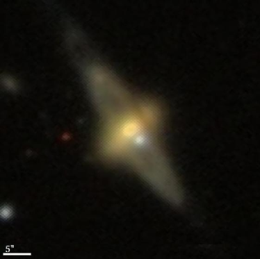
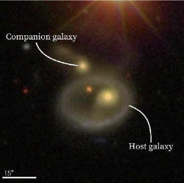
Figure 1: SDSS colour images of two objects under study. Left: polar-ring galaxy SPRC-69 (Moiseev et al. 2011). Right: IIHz4 (No 365 in Buta 2017) showing the identification of a ring host and a companion.

2.3 Data

After the PRG and CRG samples were constructed, for each galaxy necessary data from SDSS (DR16, Ahumada et al. 2020) was extracted. This includes dereddened (Schlafly & Finkbeiner, 2011) apparent magnitudes in $r$ and $g$ bands as well as spectroscopic redshifts. For galaxies whose redshift has not been measured by SDSS we used values provided in the NED if present. In this study, we consider only galaxies with spectroscopic redshifts as photometric ones may have large uncertainties which can lead to incorrect estimation of LF.

As the final selection criteria we applied $r$-band magnitude limit $m_{lim}=17.77$ following SDSS Legacy Survey Target Selection algorithm. This restriction left 103 PRGs and 74 CRGs in consideration. Table 1 summarises the final composition of our samples. The last column shows the number of objects left in consideration after all selection criteria were applied. Absolute magnitudes and colours of all galaxies were corrected using the $k$-correction calculator by Chilingarian et al. (2010). Distributions of the main characteristics of the PRGs and CPGs in our samples are presented in Figure 2.

Table 1: Description of the ringed galaxies samples used in our study

Sample	Source	Number of galaxies
PRG	Whitmore et al. (1990)	5
	Moiseev et al. (2011)	75
	Reshetnikov & Mosenkov (2019)	23
		$\Sigma\,$= 103
CRG	Madore et al. (2009)	19
	Nair & Abraham (2010)	13
	Buta (2017)	13
	Timmis & Shamir (2017)	17
	Shamir (2020)	12
		$\Sigma\,$= 74

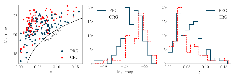
Figure 2: Left panel: Distribution of PRGs and CRGs in (M_r,z) plane, black line shows limiting apparent magnitude. Middle and right panels show the distribution of the samples galaxies by absolute magnitude and redshift respectively.

3 Luminosity function

3.1 Completeness of the samples

In order to investigate completeness of our samples we used classical $\left<V/V_{max}\right>$ test originally developed by Schmidt (1968). To implement this method one needs to calculate two values for each galaxy: $V$ – comoving volume of a sphere which radius is the distance to the object and $V_{max}$ – comoving volume of a sphere with radius corresponding to the maximum distance the galaxy could have and still be included in our sample. Assuming homogeneous distribution of objects in space, the expected value of $\left<V/V_{max}\right>$ for a complete sample is 0.5. In our case, this value equals to 0.196$\pm$0.028 for polar-ring galaxies sample and 0.087 $\pm$0.034 for collisional ring galaxies sample. These results imply that the samples are far from complete and the necessary corrections should be applied.

A number of techniques have been developed to make such corrections, we have adopted method from Huchra & Sargent (1973) as the most consistent with the used completeness test. Another advantage of this method is that it does not require to decrease the number of galaxies in the sample or model the selection process. To apply this correction one needs to tabulate $\left<V/V_{max}\right>$ over a suitable interval of $m_{lim}$ and then determine what number of galaxies should be added to keep $\left<V/V_{max}\right>$ close to 0.5. A total of 65 polar-ring galaxies are missing from our sample so we need to multiply calculated space density and luminosity function by a correction factor $\xi_{PRG}=168/103=1.63$. Respective values for collisional sample are 60 galaxies and $\xi_{CRG}=1.81$.

We note that the main drawback of this method is its integral nature, i.e. only the overall number of galaxies is corrected but not the relative number of bright and faint galaxies. This means that only the normalisation of the LF is affected but not its shape.

3.2 Methods description

Through the years a lot of different techniques have been proposed to estimate luminosity function of galaxies (see Johnston 2011). In this study, we adopted 3 classical nonparametric methods: $1/V_{max}$ (Schmidt, 1968), C^- (Lynden-Bell, 1971) and Chołoniewski method (Chołoniewski 1986). Although these methods are pretty old they have a number of important features: firstly, these techniques were repeatedly used and tested so their statistical properties are well studied (e.g. Willmer 1997; Takeuchi et al. 2000). The second advantage of using these methods is that they were established to estimate LF and space density of small samples which is the case in this study. Of course, there are certain drawbacks associated with the use of these estimators: $1/V_{max}$ can overestimate faint end of luminosity function, original C^- method does not provide normalisation and Chołoniewski’s method requires solving a nonlinear system of equations. However, there are ways to overcome such difficulties.

In order to quantify the shape of derived LFs we have fitted them with an analytical approximation. The most commonly used parametric form of LF was proposed by Schechter (1976):

$$\phi(M)=0.4\ln(10)\phi^{*}\left(10^{0.4(M^{*}-M)}\right)^{\alpha+1}e^{-10^{0.4(M^{*}-M)}},$$ (1)

where $\phi^{*}$ is the normalisation, $M^{*}$ marks the position of the turn-off point and $\alpha$ gives the logarithmic slope of LF at its faint end.

3.2.1 $1/V_{max}$ method

One of the reasons this method was adopted in our study is that it allows us to compare results with previous attempts to estimate the luminosity function taken by R11 without having to account for differences in methods.

Implementation of this method goes as follows: firstly, for each galaxy in sample we calculate value of $V_{max}$ as

$$V_{max}^{i}=\frac{\Omega}{4\pi}\int_{0}^{z_{max}(M_{i})}\frac{dV}{dz}\,dz,$$ (2)

where $z_{max}(M_{i})$ is the redshift of $i$th galaxy at which its $r$-band apparent magnitude equals $m_{lim}$ and $\Omega$ is the solid angle of the sample. Then galaxies are binned by their absolute magnitude and value of differential LF in each bin can be written as

$$\phi(M)=\frac{\xi}{\Delta M}\sum_{i}\frac{1}{V^{i}_{max}},$$ (3)

where the summation is over galaxies with $M_{i}\in[M-0.5\Delta M,M+0.5\Delta M]$. For both our samples $\Delta M=0{\aas@@fstack{m}}58$, $\Omega_{PRG}=11663$ $\Box^{\rm o}$ (SDSS DR7 imaging area), $\Omega_{CRG}=14555$ $\Box^{\rm o}$ (SDSS DR14 imaging area) and the values of $\xi$ are given above.

3.2.2 C^- and Chołoniewski methods

The C^- method of Lynden-Bell (1971) uses the distribution of galaxies in the $(M,z)$ plane to probe the luminosity function. For a sorted sample under consideration one can calculate a C^- value for $j$th galaxy as the number of galaxies with $M<M_{j}$ and $z<z_{max}(M_{j})$. Using these numbers cumulative LF $\Phi(M)$ can be calculated via recurrence relation. In this work we adopted modification of this method developed by Chołoniewski (1987) as it simultaneously provides shape and normalisation of LF.

Chołoniewski (1986) method was applied in its original form.

3.3 Volume density estimators

Three different approaches were taken to evaluate the mean volume density of galaxies in our samples.

The first one is naive:

$$\bar{n}=\xi\frac{N}{V},$$ (4)

where $N$ is the size of the sample and $V$ is its total volume.

The second is LF based and can be written as

$$n_{LF}=\int_{M_{1}}^{M_{2}}\phi(M)\,dM,$$ (5)

where $M_{1}$ and $M_{2}$ give the luminosity interval in which the volume density is calculated.

The last one is so called "EEP estimator" developed by Efstathiou et al. (1988):

$$n_{EEP}=\frac{\xi}{V}\sum_{0}^{N}\frac{1}{s(z_{i})}.$$ (6)

Here $s(z)$ is a selection function defined as

$$s(z)=\frac{\int_{M_{1}}^{\min(M_{max}(z),M_{2})}\phi(M)\,dM}{\int_{M_{1}}^{M_{2}}\phi(M)\,dM}$$ (7)

where $M_{max}(z)$ is the faintest absolute magnitude detectable at redshift $z$.

3.4 Results

Figure 3 shows our results for the LF of polar-ring and collisional ring galaxies. Different symbols represent the results obtained by different methods described in Section 3.2. The best Schechter fits are plotted with dashed lines. Previous result for PRGs derived in R11 is also added to the left panel after transforming from the $B$ to $r$ filter according to Cook et al. (2014). Filled areas represent $1\sigma$ uncertainties, for C^- and Chołoniewski methods they are calculated using bootstrap sampling, for $1/V_{max}$ we adopted an analytic formula by Condon (1989). In order to better understand the shape of the LF we made 2 additional runs each time shifting luminosity bins by 0.19 mag. All three runs (one with original bins and two with shifted bins) are presented on Figure 3.

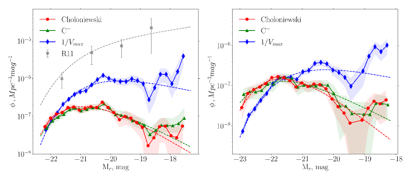
Figure 3: Luminosity function of PRGs (left panel) and CRGs (right panel). The diamonds, triangles, and circles represent the results obtained with the $1/V_{max}$, C^- and Chołoniewski methods, respectively. The filled areas show the 1$\sigma$ confidence regions of the LFs. The dashed lines describe the analytic approximations with parameters listed in Table 2. The result from R11 is also added on the left panel.

It is apparent from this figure that the estimates produced by C^- and Chołoniewski methods show good agreement for both samples whereas results from $1/V_{max}$ significantly deviates from them. According to Takeuchi et al. (2000) such difference may indicate that a density inhomogeneity is present in our samples, as $1/V_{max}$ method is affected by density fluctuations unlike the other two. The best-fit parameters of the Schechter function for each method are presented in Table 2.

As can be seen in Figure 3, the LF of PRGs from R11 is much higher than the luminosity function found in this work. The main reasons for this may be both the incompleteness of the R11 sample and its contamination with objects that are not PRGs (e.g., mergers, interacting galaxies). The R11 sample is based on the PRC and it contains nearby galaxies with $z\leq 0.05$ mostly (see fig. 7 in the SPRC). In a modest sample limited by a small spatial volume, the luminosity function can be strongly distorted by the influence of spatial inhomogeneities.

To check the influence of the redshift constraints on the LF found by the $1/V_{max}$ method, we built the LF of PRGs for subsamples with $z\leq 0.05$ and $z<0.03$ on the basis of our data. We found that as the redshift of the sample decreases, the weak wing of the luminosity function ($M_{r}\geq-20^{m}$) rises significantly (by several times). Therefore, the sensitivity of the $1/V_{max}$ method to the presence of spatial fluctuations, as well as the incompleteness of the sample of galaxies, apparently influenced the results of R11.

Table 2: Schechter function best-fit parameters

Sample	Method	$\log_{10}(\phi^{*},\,$Mpc${}^{-3})$	$M^{*}$	$\alpha$
PRG	Chołoniewski	-6.28$\pm$0.02	-20.71$\pm$0.13	0.21$\pm$0.13
	C-	-6.31$\pm$0.02	-20.78$\pm$0.12	0.05$\pm$0.10
	$1/V_{max}$	-5.66${}_{-0.05}^{+0.04}$	-20.49$\pm$0.11	-0.53$\pm$0.13
CPG	Chołoniewski	-6.42$\pm$0.03	-21.20$\pm$0.13	0.54$\pm$0.17
	C-	-6.42$\pm$0.03	-21.63$\pm$0.14	0.11$\pm$0.13
	$1/V_{max}$	-6.23${}_{-0.06}^{+0.05}$	-21.17$\pm$0.14	-0.58$\pm$0.18

Figure 4 shows LFs for red ($g-r>+0.8$, 65 galaxies) and blue ($g-r<+0.8$, 38 galaxies) PRGs. The whole procedure described above was applied to these subsamples, then the weighted mean of results produced by inhomogeneity-insensitive methods (C^- and Chołoniewski) was calculated for both groups. As can be seen in the figure, the LFs of the two types of galaxies are different. Red galaxies show a maximum and decrease towards bright and faint luminosities, the LF of blue galaxies looks more flat. Among bright objects, red galaxies dominate: in the luminosity range $-20^{m}\geq M_{r}\geq-22^{m}$, red galaxies are found 1.7 times more frequent than blue ones. Among faint objects, the contributions of blue and red PRGs are comparable.

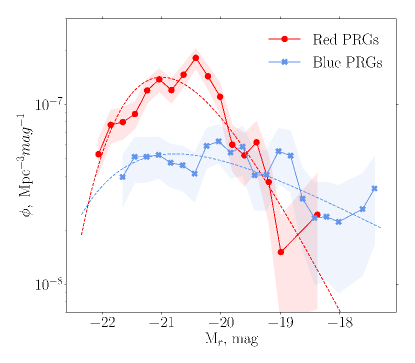
Figure 4: Mean luminosity functions of red PRGs (red circles) and blue PRGs (light blue crosses). The filled areas show the 1$\sigma$ confidence regions. Dashed lines represent best-fit Schechter functions.

The mean LFs of PRGs and CPGs are compared in Figure 5. (As described above, the mean LFs were obtained as the weighted average of C^- and Chołoniewski methods.) Both LFs exhibit similar behaviour with a gradual fall-off at low and high luminosities. Luminosity function of CPGs appears to be shifted to higher luminosities compared to the LF of PRGs. This shift is also clearly visible from the data in Table 2 – characteristic absolute magnitudes $M^{*}$ for CPGs are brighter by $0{\aas@@fstack{m}}5-0{\aas@@fstack{m}}8$ compared to PRGs.

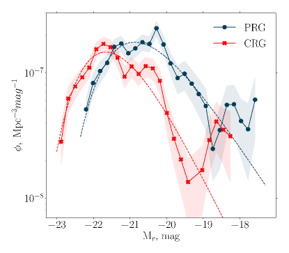
Figure 5: Mean luminosity functions of PRGs (blue circles) and CRGs (red crosses). The filled areas show the 1$\sigma$ confidence regions. Dashed lines represent best-fit Schechter functions.

Once the luminosity functions were computed, volume density could be evaluated employing estimators described in Section 3.3. The obtained values are presented in Table 3. We see that all estimates are consistent with each other. (In Table 3 and below the results of the $1/V_{max}$ method are not used – see discussion above).

Table 3: Volume density of PRGs and CRGs obtained by different estimators

Sample	LF Method	$n_{EEP},10^{-7}\,$Mpc-3	$n_{LF},10^{-7}\,$Mpc-3	$\bar{n},10^{-7}\,$Mpc-3
PRG	Chołoniewski	$6.74_{-0.60}^{+0.93}$	$5.17\pm 1.59$
	C-	$7.02_{-0.60}^{+0.86}$	$5.23\pm 1.78$	$4.94$
CPG	Chołoniewski	$4.04_{-0.16}^{+0.27}$	$3.61\pm 1.12$
	C-	$4.29_{-0.27}^{+0.45}$	$3.57\pm 1.24$	$3.62$

The values we found – $n_{0}(PRGs)\approx(5-7)\times 10^{-7}$ Mpc^-3 and $n_{0}(CPGs)\approx 4\times 10^{-7}$ Mpc^-3 – are noticeably smaller than those previously published. According to our estimates, the relative fraction of apparent PRGs is $\sim 10^{-4}$ of all galaxies; collisional rings are about 1.5 times as rare as PRGs.

It should be noted that the value of $n_{0}$ for PRGs is the lower limit of the real frequency of such galaxies. As can be clearly seen from the PRC and SPRC catalogues, PRGs are predominantly identified in cases where the polar structure is seen at a large angle to the line of sight, almost edge-on. As Whitmore et al. (1990) noted, for every obvious PRG there are two other PRGs that are missed. Thus, the actual fraction of PRGs must be larger by approximately a factor of 3. Also, collision rings are easier to detect when they are seen almost face-on. Therefore, the true volume density of CRGs should be slightly higher than we have estimated.

4 Density evolution

If we know the local volume density of galaxies, we can estimate the redshift evolution of this density. Implying some evolutionary model, for a given solid angle of the sky field $\Omega$ and redshift range (from $z_{1}$ to $z_{2}$) one can calculate the expected number of objects as

$$N_{exp}=\Omega\int_{z_{1}}^{z_{2}}n(z)\,\frac{dV}{dz}dz,$$ (8)

where $dV$ is a comoving volume element.

Volume density evolution is usually described by a simple power law $n(z)=n_{0}\cdot(1+z)^{m}$, where $n_{0}$ is the local density of objects under consideration. Then, comparing $N_{exp}$ to the observed number of objects in the field, the $m$ exponent can be evaluated.

4.1 Polar-ring galaxies

Up to date only three distant polar-ring galaxy candidates are known located in the Hubble Deep Field North (HDF-N) and the Hubble Ultra-Deep Field (HUDF); none were identified in the Hubble Deep Field South (Reshetnikov 1997; Reshetnikov & Dettmar 2007).

HDF-N contains two candidates to PRGs. One galaxy (HDF-N 2-809) in its morphology is similar to the nearby polar-ring galaxy NGC 4650A, and the second (HDF-N 2-906) resembles NGC 2685 (Reshetnikov 1997). The first galaxy is at redshift $z=0.71$, the second one is at redshift $z=1.24$ (Yang et al. 2014). The third galaxy is in the HUDF (HUDF 1619, see Reshetnikov & Dettmar 2007) at redshift $z=1.30$ (Rafelski et al. 2015).

The total area of three deep fields (HDF-N + HDF-S + HUDF) is $1.89\times 10^{-6}$ sr. Adopting the local volume density of PRGs $n_{0}(PRGs)=6\times 10^{-7}$ Mpc^-3 (Table 3), we found that in the case of no evolution ($m=0$) the expected number of PRGs over the redshift interval of $0\leq z\leq 1.3$ in the directions of three deep fields is only 0.02. Assuming Poisson errors, observed number of polar rings is consistent with an exponent value of $m=7.0_{-1.2}^{+0.6}$ This means a very steep increase of PRGs volume density with redshift.

Finkelman et al. (2010) found a candidate for PRG in the Subaru Deep Field (SDF) at $z=0.061$. Assuming $\Omega(SDF)=7.62\times 10^{-5}$ sr, $z\leq 0.1$ and $m=0$, we determined the expected number of PRGs as 0.001. In order to find one PRG in the direction of SDF, it is necessary to accept an extremely high rate of evolution with $m>>10$. Presence of one candidate for PRG in the VST Deep Field (Iodice et al. 2015a) at $z=0.051$ also leads to an estimate of $m>>10$.

Therefore, the current very scarce statistics on the frequency of PRGs provide indications of the possibility of a rapid evolution of the spatial density of such galaxies up to $z\sim 1$.

4.2 Collisional ring galaxies

Statistics of high-redshift collisional ring galaxies is much richer. Lavery et al. (1996) identified 7 P-type rings in the HST images of the Tucana dwarf galaxy. Additional 25 CRGs were spotted in deep images from the HST archives by Lavery et al. (2004). Later, Elmegreen & Elmegreen (2006) listed 24 collisional rings and 15 “bent chains” found in GOODS and GEMS fields.

Combining these 3 sources and discarding bent chains (as they morphologically differ from our local CRG sample) we get 56 galaxies with $0.0<z\leq 1.4$ located in the total area of $1.39\times 10^{-4}$ sr. Corresponding local density $n_{0}=4\times 10^{-7}\,$Mpc^-3 (Table 3). In a nonevolving case the expected number of CRGs in these fields is 1 and the value of $m$ corresponding to the observed number of objects is $5.2_{-0.2}^{+0.2}$ which is consistent with results obtained by Lavery et al. (2004).

It should be noted that although local densities obtained by C^- and Chołoniewski’s methods are somewhat different, these variations do not affect $m$ significantly. If we pick any of four estimations, the value of $m$ would vary by less than 5%.

5 Conclusions

Based on the SDSS data, we constructed the luminosity functions for two types of ringed galaxies – polar-ring galaxies and collisional ring galaxies. Both types of galaxies are natural consequences of galactic collisions (CPGs), interactions and external accretion of matter (PRGs). Consequently, the statistics of such objects at different $z$ can be used to estimate the rate of galaxy interactions in different epochs.

We used different approaches to evaluate LF. Two of them (C^- and Chołoniewski methods) showed good agreement, method $1/V_{max}$, sensitive to density inhomogeneities, gave overestimated LF values. Our main conclusions are based on the results of the first two approaches.

– LFs of ringed galaxies have global maxima and falling wings at high and low luminosities (Figure 5). LF of CRGs is shifted towards higher luminosities compared to PRGs. The decrease in the number of PRGs and CRGs at low luminosities may be due to the fact that the formation of large-scale optical polar structures and extended collisional rings is more likely in non-dwarf galaxies. As for PRGs, our conclusion is in general agreement with the results of Zhou et al. (2022), who found that the fraction of kinematically misaligned galaxies declines to both low and high mass end.

– Polar structures are more common in red (early-type) galaxies compared to blue ones (Figure 4). This is consistent with direct estimates of the morphological types of PRGs (e.g. Whitmore 1991). This result looks natural, since the polar structures around spiral galaxies with extended gaseous discs should exist for a shorter time compared to gas-free red ones. (However, polar structures also exist around spiral galaxies – see discussion in Moiseev 2014).

– Very poor statistics of distant PRGs does not contradict the assumption of a rapid evolution of their volume density to $z\sim 1$ (Sect. 4.1). Since the rate of interactions and mergers of galaxies increases with redshift (e.g. Conselice et al. 2009), our result is in agreement with the standard assumption that formation of PRGs is associated with their interactions with the environment: major and minor merging, tidal accretion of matter from nearby galaxy, infall of gas from intergalactic space (e.g. Bekki 1997; Reshetnikov & Sotnikova 1997; Maccio et al. 2006).

– Current statistics of CRGs confirms the rapid increase in their volume density towards $z\sim 1$ (Sect. 4.2). This rapid increase may reflect an increase in the rate of high-speed collisions of galaxies, leading to the formation of such objects. On the other hand, this growth is apparently not monotonic. According to Yuan et al. (2020), the volume vensity of massive CPGs at $z\approx 2$ can be comparable to the same density in the nearby Universe. (This decline may be due to a decreased fraction of large spiral galaxies at high redshift.) Non-monotonic behavior of the interaction/merger rate evolution is consistent with the data obtained for other types of objects (e.g. Conselice et al. 2008, 2022); however, the statistics of CPGs at highest $z$ is still insufficient for meaningful conclusions.

The results of our work show that polar-ring and collisional ring galaxies can be useful indicators of the rate of interactions at high redshifts. Nevertheless, for the successful use of these indicators, it is necessary to significantly increase the statistics of such objects in the local Universe and at different $z$.

Modern wide-field sky surveys (SDSS, Pan-STARRS, Legacy, etc.) provide morphological and photometric information on millions of galaxies, which requires computer analysis methods to select and recognize the desired objects. Such studies are now being carried out (for example, Timmis & Shamir 2017) and it is hoped that in the coming years our knowledge of nearby galaxies (including PRGs and CPGs) will improve significantly.

The main tool for studying the distant Universe in the coming years is the James Webb Space Telescope. The operation of this telescope will make it possible to detect a large number of ringed galaxies at high redshifts, similar to the one discovered by Yuan et al. (2020) at $z=2.19$. The combination of these data will make it possible to trace the evolution of ringed galaxies over cosmological times.

Data availability

The data underlying this article will be shared on reasonable request to the corresponding author.

References

- Abraham et al. (1996) Abraham R.G., van den Bergh S., Glazebrook K., Ellis R.S., Santiago B.X., Surma P., Griffiths R.E., 1996, ApJS, 107, 1
- Ahumada et al. (2020) Ahumada R., Prieto C. A., Almeida A., Anders F., Anderson S. F., Andrews B. H., Anguiano B., et al., 2020, ApJS, 249, 3
- Appleton & Struck-Marcell (1996) Appleton P.N., Struck-Marcell C., 1996, Fund. Cosm. Phys., 16, 111
- Arp & Madore (1987) Arp H. C., Madore B., 1987, A Catalogue of Southern Peculiar Galaxies and Associations. Cambridge Univ. Press, Cambridge
- Bekki (1997) Bekki K., 1997, ApJ, 490, L37
- Binggeli et al. (1988) Binggeli B., Sandage A., Tammann G.A., 1988, ARA&A, 26, 509
- Bizyaev et al. (2014) Bizyaev D. V., Kautsch S. J., Mosenkov A. V., Reshetnikov V. P., Sotnikova N. Y., Yablokova N. V., Hillyer R. W., 2014, ApJ, 787, 24.
- Blanton et al. (2003) Blanton M.R., Hogg D.W., Bahcall N.A., et al., 2003, ApJ, 592, 819
- Bournaud & Combes (2003) Bournaud F., Combes F., 2003, A&A, 401, 817
- Bridge et al. (2010) Bridge C.R., Carlberg R.G., Sullivan M., 2010, ApJ, 709, 1067
- Brook et al. (2008) Brook Ch.B., Governato F., Quinn Th., et al., 2008, ApJ, 689, 678
- Buta (2017) Buta R. J., 2017, MNRAS, 471, 4027
- Chambers et al. (2016) Chambers K. C., Magnier E. A., Metcalfe N., Flewelling H. A., Huber M. E., Waters C. Z., Denneau L., et al., 2016, arXiv:1612.05560
- Cheng et al. (2020) Cheng T.-Y., Conselice C. J., Aragón-Salamanca A., Li N., Bluck A. F. L., Hartley W. G., Annis J., et al., 2020, MNRAS, 493, 4209.
- Chilingarian et al. (2010) Chilingarian I. V., Melchior A.-L., Zolotukhin I. Y., 2010, MNRAS, 405, 1409
- Chołoniewski (1986) Chołoniewski J., 1986, MNRAS, 223, 1
- Chołoniewski (1987) Chołoniewski J., 1987, MNRAS, 226, 273
- Condon (1989) Condon J. J., 1989, ApJ, 338, 13
- Conselice et al. (2008) Conselice Ch.J., Rajgor Sh., Myers R., 2008, MNRAS, 386, 909
- Conselice et al. (2009) Conselice Ch.J., Yang C., Bluck A.F.L., 2009, MNRAS, 394, 1956
- Conselice et al. (2022) Conselice Ch.J., Mundy C.J., Ferrera L., Duncan K., 2022, arXiv:2207.03984
- Cook et al. (2014) Cook D.O., Dale D.A., Johnson B.D., et al., 2014, MNRAS, 445, 890
- D′Onghia et al. (2008) D′Onghia E., Mapelli M., Moore B., 2008, MNRAS, 389, 1275
- Duncan et al. (2019) Duncan K., Conselice Ch., Mundy C., et al., 2019, ApJ, 876, 110
- Efstathiou et al. (1988) Efstathiou G., Ellis R. S., Peterson B. A., 1988, MNRAS, 232, 431
- Egorov & Moiseev (2019) Egorov O.V., Moiseev A.V., 2019, MNRAS, 486, 4186
- Elagali et al. (2018) Elagali A., Lagos C.D.P., Ivy Wong O., et al., 2018, MNRAS, 481, 2951
- Elmegreen & Elmegreen (2006) Elmegreen D. M., Elmegreen B. G., 2006, ApJ, 651, 676
- Felten (1977) Felten J.E., 1977, AJ, 82, 861
- Fernandez et al. (2021) Fernandez J., Alonso S., Duplancic F., Coldwell G., 2021, A&A, 653, A71
- Few & Madore (1986) Few J.M.A., Madore B.F., 1986, MNRAS, 222, 673
- Finkelman et al. (2010) Finkelman I., Graur O., Brosch N., 2010, MNRAS, 208, 2010
- Fukugita et al. (1998) Fukugita M., Hogan C.J., Peebles P.J.E., 1998, ApJ, 503, 518
- Fukugita & Kawasaki (2022) Fukugita M., Kawasaki M., 2022, MNRAS, 513, 8
- Huchra & Sargent (1973) Huchra J., Sargent W. L. W., 1973, ApJ, 186, 433
- Iodice et al. (2015a) Iodice E., Capaccioli M., Spavone M., et al., 2015a, A&A, 574, A111
- Iodice et al. (2015b) Iodice E., Coccato L., Combes F., et al., 2015b, A&A, 583, A48
- Johnston (2011) Johnston R., 2011, A&ARv, 19, 41
- Lavery et al. (1996) Lavery R. J., Seitzer P., Suntzeff N. B., Walker A. R., Da Costa G. S., 1996, ApJL, 467, L1
- Lavery et al. (2004) Lavery R. J., Remijan A., Charmandaris V., Hayes R. D., Ring A. A., 2004, ApJ, 612, 679
- Lintott et al. (2011) Lintott Ch., Schawinski K., Bamford S., et al. 2011, MNRAS, 410, 166
- López-Sanjuan et al. (2009) L opez-Sanjuan C., Balcells M., Pérez-González P.G., et al., 2009, A&A, 501, 505
- Lotz et al. (2011) Lotz J.M., Jonsson P., Cox T.J., et al., 2011, ApJ, 742, 103
- Lotz, Primack, & Madau (2004) Lotz J. M., Primack J., Madau P., 2004, AJ, 128, 163
- Lynden-Bell (1971) Lynden-Bell D., 1971, MNRAS, 155, 95
- Maccio et al. (2006) Maccio A.V., Moore B., Stadel J., 2006, ApJ, 636, L25
- Madore et al. (2009) Madore B.F., Nelson E., Petrillo K., 2009, ApJS, 181, 572
- Makarov et al. (2022) Makarov D., Savchenko S., Mosenkov A., Bizyaev D., Reshetnikov V., Antipova A., Tikhonenko I., et al., 2022, MNRAS, 511, 3063
- Mapelli et al. (2008) Mapelli M., Moore B., Ripamonti E., et al., 2008, MNRAS, 383, 1223
- Marchuk et al. (2022) Marchuk A. A., Smirnov A. A., Sotnikova N. Y., Bunakalya D. A., Savchenko S. S., Reshetnikov V. P., Usachev P. A., et al., 2022, MNRAS, 512, 1371.
- Mitronova et al. (2004) Mitronova S. N., Karachentsev I. D., Karachentseva V. E., Jarrett T. H., Kudrya Y. N., 2004, BSAO, 57, 5
- Moiseev (2014) Moiseev A., 2014, ASP Conf. Ser., 486, 61
- Moiseev et al. (2011) Moiseev A.V., Smirnova K.I., Smirnova A.A., Reshetnikov V.P., 2011, MNRAS, 418, 244 (SPRC)
- Nair & Abraham (2010) Nair P. B., Abraham R. G., 2010, ApJS, 186, 427
- Pearson et al. (2022) Pearson W.J., Suelves L.E., Ho S.C.-C., et al., 2022, A&A, 661, A52
- Rafelski et al. (2015) Rafelski M., Teplitz H.I., Gardner J.P., et al., 2015, AJ, 150, 31
- Reshetnikov (1997) Reshetnikov V. P., 1997, A&A, 321, 749
- Reshetnikov & Sotnikova (1997) Reshetnikov V., Sotnikova N., 1997, A&A, 325, 933
- Reshetnikov & Dettmar (2007) Reshetnikov V. P., Dettmar R.-J., 2007, AstL, 33, 222
- Reshetnikov et al. (2011) Reshetnikov V. P., Faúndez-Abans M., de Oliveira-Abans M., 2011, AstL, 37, 171 (R11)
- Reshetnikov & Mohamed (2011) Reshetnikov V. P., Mohamed Y.H., 2011, AstL, 37, 743 (arXiv:1109.6159)