Current address: ]CESAM Research Unit, University of Liège, 4000 Liège, Belgium
Many-body interference at the onset of chaos
Abstract
We unveil the signature of many-body interference across dynamical regimes of the Bose-Hubbard model. Increasing the particles’ indistinguishability enhances the temporal fluctuations of few-body observables, with a dramatic amplification at the onset of quantum chaos. By resolving the exchange symmetries of partially distinguishable particles, we explain this amplification as the fingerprint of the initial state’s coherences in the eigenbasis.
Interacting many-particle dynamics may be considered the most plausible origin of instabilities, chaos and complexity, from astronomical Chirikov and Vecheslavov (1989); Laskar and Gastineau (2009) to microscopic Bohr (1936) scales. Due to the rapid growth of phase space with the particle number, together with its progressively more intricate topology, deterministic descriptions quickly hit the ceiling, enforcing statistical descriptions. Some type of coarse graining, implicit to such approaches, allows classifications of dynamical behavior—e.g., as scale-invariant, chaotic or Markovian—associated with universal characteristics which are formalized, e.g., in the theories of phase transitions Landau and Lifschitz (1984); Sachdev (2011), random matrices (RMT) Mehta (1991), or open quantum systems Davies (1976); Alicki and Lendi (1987); Breuer and Petruccione (2002). It is the universal character of these features which allows robust predictions, since full resolution of complex dynamics is prohibitive, by their very nature.
On the quantum level, robust features are in such scenarios essentially controlled by spectral densities and statistics, the localization properties of eigen- and initial states, the phase-space dimension, and the time scales over which to make predictions. This is the unifying view of quantum chaos Giannoni et al. (1989), which has proven enormously versatile an approach to analyze complex quantum systems—including paradigmatic many-particle scenarios in nuclear Guhr and Weidenmüller (1989); Rotter (1991) and atomic physics Holle et al. (1988); Iu et al. (1991); Krug and Buchleitner (2001), as well as in cold matter Moore et al. (1995); Wimberger et al. (2004); Meinert et al. (2014); Kaufman et al. (2016) and black hole Liu and Vardhan (2021) contexts. On this level of description, the specific many-particle nature of the underlying Hamiltonian does not appear as an essential ingredient anymore, since all the features of complex dynamics can also be observed on the level of single-particle dynamics Giannoni et al. (1989); Garbaczewski and Olkiewicz (2002) (provided the phase space dimension is large enough—such that tori are not isolating anymore v. Milczewski et al. (1996)).
Yet, quantum systems composed of identical particles undeniably exhibit properties that fundamentally distinguish them from classical many- and single-particle systems, hardwired in exchange symmetries Landau and Lifschitz (1985); Tichy and Mølmer (2017), and generating many-body interference (MBI) phenomena Hong et al. (1987); Tichy et al. (2010); Dufour et al. (2017); Shchesnovich and Bezerra (2018); Giordani et al. (2018); Dittel et al. (2018a, b); Brünner et al. (2018); Jones et al. (2020); Dufour et al. (2020); Dittel et al. (2021); Brunner et al. ; Tichy et al. (2012); Stanisic and Turner (2018); Dufour et al. (2020); Dittel et al. (2021), thus with potentially dramatic dynamical relevance. In fact, modern experiments Greiner et al. (2002); Bloch et al. (2008); Gericke et al. (2008); Gemelke et al. (2009); Karski et al. (2009); Bakr et al. (2010); Sherson et al. (2010); Kaufman et al. (2016); Lukin et al. (2019); Rispoli et al. (2019) already allow to control external and internal degrees of freedom (dof) of many-particle quantum systems, such that physically identical particles may be equipped with a continuously tunable degree of partial distinguishability (PD), and, by this, to ultimately control the impact of MBI on the dynamics Brünner et al. (2018); Dufour et al. (2020); Dittel et al. (2021); Brunner et al. . While, traditionally, the RMT approach deliberately divides out any symmetry-induced properties Giannoni et al. (1989); Mehta (1991) (see, however, Giraud et al. (2022)), it is clear that MBI, as a manifestation of the specific system’s particle exchange symmetry, is one of those robust features which need to be accounted for in any theory of complex quantum systems. This raises the question: Where in a many-body quantum system’s spectral and eigenstate structure is MBI encoded, and how can we distill its impact on observable dynamical properties?
In this contribution, we identify a signature of bosonic MBI in the asymptotic temporal fluctuations of expectation values around their average. We show that is controlled by the coherences of the many-particle initial state in the eigenbasis, multiplied by the corresponding off-diagonal elements of the observable, and is therefore strongly enhanced by particle indistinguishability. We extract from the quench dynamics of a Mott state in the Bose-Hubbard model for increasing values of tunnelling strength . As shown in Fig. 1, is sharply peaked around the value of where the dynamics becomes chaotic. There, the initial state is sufficiently delocalized in the eigenbasis for coherences to build up, but not so much that they are cut off by the finite energy bandwidth of the observable. By taking into account the eigenstates’ structure as constrained by their symmetry under particle exchange, we find the strongest dependence of on the particles’ mutual (in)distinguishability precisely at that point. Given the very general ingredients of our theoretical analysis, we conclude that many-body coherence effects are most intense at the onset of quantum chaos.
We consider the one-dimensional Bose-Hubbard model Fisher et al. (1989); Lewenstein et al. (2007); Bloch et al. (2008); Cazalilla et al. (2011); Krutitsky (2016) of PD particles with hard-wall boundary conditions,
| (1) |
which is experimentally realizable with ultracold atoms in optical lattices Greiner et al. (2002); Bloch et al. (2008); Gericke et al. (2008); Gemelke et al. (2009); Karski et al. (2009); Bakr et al. (2010); Sherson et al. (2010); Kaufman et al. (2016); Lukin et al. (2019); Rispoli et al. (2019). The first index of the creation and annihilation operators refers to the Wannier orbitals of the lattice, which span the external single-particle Hilbert space . The second index refers to a basis of the -dimensional internal single-particle Hilbert space, describing, e.g., the electronic state of an atom loaded into an optical lattice. The operator counts the number of particles on lattice site , irrespective of their internal state. We keep the total particle number fixed. The two terms in describe nearest-neighbor tunneling and on-site interaction of the particles, both of which act exclusively on the external dof, while the internal dof remain static. For indistinguishable bosons, depending on the relative contribution of both terms in (1), a quantum-chaotic region has been identified both from spectral statistics and eigenstate delocalization Buchleitner and Kolovsky (2003); Kolovsky and Buchleitner (2004); Kollath et al. (2010); Beugeling et al. (2015); Dubertrand and Müller (2016); Kaufman et al. (2016); Beugeling et al. (2018); Lukin et al. (2019); Rispoli et al. (2019); Pausch et al. (2021a, b, 2022). We here establish its existence also for PD particles, as an important corollary of our subsequent analysis.
Of experimental interest are few-particle observables, e.g., low-order density correlations . Formally, these are given by products of creation and annihilation operators Brünner et al. (2018); Dufour et al. (2020), , such that they only access the marginal information inscribed in the -particle (P) reduced state Brunner (2019); Brunner et al. . Moreover, like the Hamiltonian, these observables are assumed to exclusively act on external dof, such that we can consider their restriction to and trace out the internal dof from the full system state to obtain Brunner (2019); Dittel et al. (2021); Brunner et al. . Partial distinguishability of the particles results in entanglement between their external and internal dof Brunner et al. ; Dittel et al. (2021), and we use as a measure of indistinguishability the purity of the external state, which is maximal () for indistinguishable particles, and minimal for perfectly distinguishable ones Brunner (2019); Dittel et al. (2021).
The system’s dynamical equilibration, on asymptotic time scales, is captured by the temporal variance of expectation values :
| (2) |
where indicates the average over the positive time axis SM . To formulate general statements, independent of the specific choice of observable , we consider an unbiased average (indicated by ) over an orthonormal basis of the (finite-dimensional) Hilbert space of external P observables N (1),
| (3) |
This quantity is shown, for , in Fig. 1 (top panel), for the dynamics generated by (1), with , initially one particle per external mode, versus the control parameter . A variable level of PD is obtained by random generation SM of the particles’ internal states , , of the initial Mott state, such as to smoothly cover the entire range .
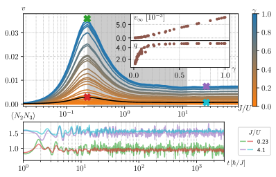
We observe that, for all , monotonically grows with , i.e., as MBI contributions are enhanced. Moreover, exhibits a maximum at , and then decreases to a plateau value with increasing . The peak is located at the transition to the (grey shaded) parameter range where (1) exhibits fully developed quantum chaos, as identified by the ergodicity properties of its eigenstates (see discussion of Fig. 2(c) below). Both and the enhancement of the fluctuations at the peak increase monotonically with , as shown in the inset. In particular, steeply increases at small , when MBI starts to kick in, which signals a particularly strong sensitivity to MBI at the transition to quantum chaos. We observe the same qualitative behavior (see SM ) for the experimentally more accessible average over all two-point density correlations Giordani et al. (2018); Walschaers et al. (2016). In the bottom panel of Fig. 1, we also give the long-time series of , for four values of and , with strongest fluctuations for intermediate and , in agreement with the above. The peak in the fluctuations at the onset of chaos can be qualitatively explained by the competition between the initial state’s delocalization and the observable’s bandwidth in the eigenbasis, as sketched in the top panels of Fig. 2(b). However, a precise discussion requires to first consider the particle-exchange symmetry of PD bosons, which is at the origin of the overall increase of with indistinguishability .
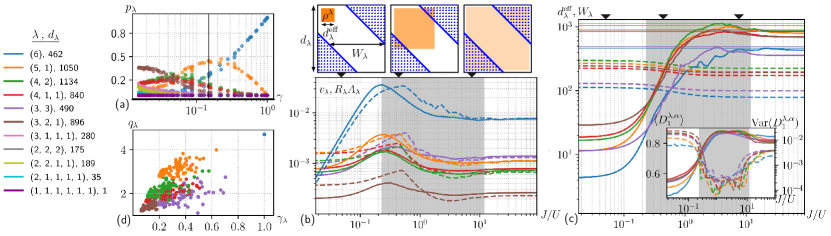
States of PD bosons are characterized by the coexistence of several types of mixed particle-exchange symmetries, alongside the fully symmetric, bosonic symmetry Tichy and Mølmer (2017); Dufour et al. (2020). The suppression of as we make particles more distinguishable (i.e., for decreasing ) can be understood by the emergence of such non-bosonic contributions to the dynamics. Indeed, group representation theory, and specifically the Schur-Weyl duality Fulton and Harris (2004); Rowe et al. , tell us that , and (as operators on ) decompose into symmetry sectors labelled by the integer partitions of (or Young diagrams): . While states of perfectly indistinguishable bosons are entirely supported on the bosonic sector, , states of PD particles also have finite weights on the other sectors (), as shown in Fig. 2(a) for states with variable levels of indistinguishability (as used as initial states in Fig. 1). Every sector further decomposes SM into identical blocks, each of dimension , and we denote by the Young basis Fulton and Harris (2004); Dufour et al. (2020), built upon the Wannier basis, of one such block. Diagonalizing in this very block, we find the eigenstates , with respect to which we represent the observable and the initial state, and . With this definition, the matrix has unit trace. If we denote its purity by , the purity of reads .
The above structure allows to decompose , as given by Eq. (3), into contributions from individual symmetry sectors. In the absence of degeneracies between energy levels and between energy gaps, within each block and between -sectors, we obtain SM
| (4) |
The individual contributions are determined by the squared weights , and by the off-diagonal elements of initial state and observable in the eigenbasis. For indistinguishable particles, and , the fluctuations are thus governed by purely bosonic MBI. As decreases, the state starts to distribute over other sectors, as shown in Fig. 2(a). The fluctuations are then doubly suppressed: through the squared weights in Eq. (4), and because of for all , as we will show in Fig. 2(b). In the limit of distinguishable particles (smallest ), the state is distributed over all sectors and is minimal.
To elucidate the origin of the maximum of at the transition to quantum chaos, we develop a simple statistical model for the off-diagonal elements of state and observable appearing in Eq. (4). We assume that the averaged matrix elements vanish outside a band of width N (2); SM , as suggested by the eigenstate thermalization hypothesis Feingold and Peres (1986); Deutsch (1991); Srednicki (1994, 1999); Hiller et al. (2006); Deutsch (2018). As for the state , we suppose that it only populates consecutive (in energy) eigenstates, as sketched in the top panels of Fig. 2(b). Otherwise, and are assumed to be statistically independent, such that we can factorize (see SM )
| (5) |
This is qualitatively underpinned by Fig. 2(b), for a state with , for the largest six symmetry sectors (which carry of ). Note that weighting those by the squares of the associated [black vertical line in Fig. 2(a)], according to Eq. (4), results in the black curve highlighted in the upper panel of Fig. 1.
We find that is, to a good approximation, independent of , and of order one in all contributing sectors N (3); SM . Consequently, the dependence of on is predominantly controlled by . From [cf. Eq. (5)] we rewrite the sum over coherences , where the inverse participation ratio is a measure of the initial state’s localization in the eigenbasis, which we now turn to.
Since provides an estimate of the number of eigenstates occupied by the initial state, we use it to define the state’s effective dimension . The multiplicative factor enforces in the regime of strongest delocalization, since, due to residual fluctuations of , generically underestimates the actual number of populated eigenstates. Figure 2(c) illustrates the delocalization of the initial state seeding the fluctuations displayed in Fig. 1, in the energy eigenbasis of the largest six sectors [carrying between (distinguishable particles) and (indistinguishable particles) of the initial state, cf. Fig. 2(a)]. From the strongly interacting limit , grows with increasing tunneling strength, reaching a maximum in most sectors in the range , before stabilizing at a value of order for .
The delocalization of the initial state in the eigenbasis mirrors the delocalization of the eigenstates in the Young basis , which signals the emergence of quantum chaos. As demonstrated in Refs. Pausch et al. (2021a, b, 2022) for indistinguishable bosons, the chaotic region can be identified by the ergodicity of eigenstates in the individual -sectors, as measured by their fractal dimension . The inset of Fig. 2(c) shows the mean value and the variance , taken over the 60 eigenstates closest in energy to the initial state, for each -sector. A substantial delocalization occurs for (shaded area), where the mean values reach their maxima, accompanied by a drop of the variances by at least one order of magnitude, attesting a strongly uniform eigenstate structure in all shown sectors. Consequently, the chaotic domain identified for indistinguishable bosons Pausch et al. (2021a) persists for mixed particle-exchange symmetry.
In contrast to the sharp growth of , the bandwidth of the observable only decreases slightly with . We estimate it by taking the standard deviation of the (normalized) distribution for each , and averaging over . Figure 2(c) shows the resulting (dashed lines) versus , in the largest six sectors.
The behavior of can then be qualitatively understood in terms of the three regimes sketched at the top of Fig. 2(b). In the limit (leftmost sketch), the initial Mott state is itself an eigenstate and decomposes on only a few (degenerate) eigenstates . Accordingly, the inverse participation ratio is maximal, yielding a minimal value of the sum over coherences , as captured by the decreasing left tails of the in Fig. 2(b). Instead, for within and beyond the range of fully developed quantum chaos (rightmost sketch), the initial state is strongly delocalized in the eigenbasis (), such that many non-zero coherences with are suppressed by multiplication with a vanishing in Eq. (4). In the factorized form Eq. (5), this effect gives rise to the denominator of , which results (with , ) in a small asymptotic value for large . At the transition between the two parameter ranges (central sketch), the onset of quantum chaos, where the eigenstates undergo a metamorphosis from localized to ergodic, triggers the initial state’s delocalization in the eigenbasis. There, exhibits a maximum, since already populates a substantial energy window, resulting in an enhanced contribution by coherences, which are, however, not yet suppressed by the observable’s bandwidth.
To explain why the effect of PD on is comparatively strongest at this maximum, we turn to the dependence of on the purity of the state associated with a given symmetry sector: We have seen that the plateau value scales linearly with . In Fig. 2(d), we observe a correlation of the sector-specific enhancement with (for those sectors contributing most), signalling a faster-than-linear scaling of the peak height with . Accordingly, the relative peak height is largest for the bosonic sector , which always has maximal purity SM . This explains the sharp growth of observed in the inset of Fig. 1 for , as the bosonic contribution to in Eq. (4) surpasses contributions from non-bosonic sectors [Fig. 2(a),(b)]. For , the bosonic contribution is dominant, as reflected by the convergence of towards [cf. inset Fig. 1].
We have thus shown that many-body coherences populated by the initial state leave a statistically robust imprint in the long-time fluctuations of few-particle observables. The emergence of the chaotic phase induces the delocalization of the initial state in the eigenbasis, translating into an augmented contribution of coherences within the observable’s energy bandwidth, and hence leading to the maximization of fluctuations. This reflects the enhanced sensitivity of a quantum system’s eigenstate structure (anchored in the underlying phase space’s topological metamorphosis Giannoni et al. (1989)) at the chaos transition, which is inherited by single- as well as by many-particle transition amplitudes Robbins (1989); Seligman and Weidenmüller (1994); Schlagheck et al. (2019). While this fluctuation maximum is observed for any degree of particle distinguishability, it is significantly amplified as the particles become more indistinguishable, because of many-body interference (MBI) contributions stemming from the bosonic symmetry sector. Therefore, full resolution of the particle-exchange symmetry sectors is indispensable to understand how MBI is seeded by the spectral and eigenstate structure of a many-body quantum system, and to discern MBI’s impact on the dynamics. Ultimately, this approach allows the discrimination of interaction-induced from entirely quantum (due to many-particle interferences) causes of dynamical complexity.
Acknowledgements.
The authors thank Dominik Lentrodt for fruitful discussions. The authors acknowledge support by the state of Baden-Württemberg through bwHPC (High Performance Computing, Baden-Württemberg), and funding by the Deutsche Forschungsgemeinschaft (DFG, German Research Foundation)—Grants No. INST 40/575-1 FUGG (JUSTUS 2 cluster) and No. 402552777. E. G. C. acknowledges support from the Georg H. Endress Foundation. E. B., L. P., and A. R. acknowledge support by Spanish MCIN/AEI/10.13039/501100011033 (Ministerio de Ciencia e Innovación/Agencia Estatal de Investigación) through Grant No. PID2020–114830GB-I00.References
- Chirikov and Vecheslavov (1989) B. Chirikov and V. Vecheslavov, Astron. Astrophys. 221, 146 (1989).
- Laskar and Gastineau (2009) J. Laskar and M. Gastineau, Nature 459, 817 (2009).
- Bohr (1936) N. Bohr, Nature 137, 344 (1936).
- Landau and Lifschitz (1984) L. Landau and E. Lifschitz, Lehrbuch der Theoretischen Physik, Band V: Statistische Physik, Teil 1 (Akademie-Verlag, Berlin, 1984).
- Sachdev (2011) S. Sachdev, Quantum Phase Transitions (Cambridge Univ. Press, Cambridge, 2011).
- Mehta (1991) M. L. Mehta, Random Matrices, 3rd ed. (Elsevier, Amsterdam, 1991).
- Davies (1976) E. Davies, Quantum theory of open quantum systems (Academic Press, New York, 1976).
- Alicki and Lendi (1987) R. Alicki and K. Lendi, Quantum Dynamical Semigroups and Applications (Springer Verlag, Berlin, 1987).
- Breuer and Petruccione (2002) H.-P. Breuer and F. Petruccione, The Theory of Open Quantum Systems (Cambridge Univ. Press, Cambridge, 2002).
- Giannoni et al. (1989) M. J. Giannoni, A. Voros, and J. Zinn-Justin, eds., Les Houches Session LII: Chaos and Quantum Physics (North-Holland, Amsterdam, 1989).
- Guhr and Weidenmüller (1989) T. Guhr and H. A. Weidenmüller, Ann. Phys. 193, 472 (1989).
- Rotter (1991) I. Rotter, Rep. Prog. Phys. 54, 635 (1991).
- Holle et al. (1988) A. Holle, J. Main, G. Wiebusch, H. Rottke, and K. H. Welge, Phys. Rev. Lett. 61, 161 (1988).
- Iu et al. (1991) C. Iu, G. R. Welch, M. M. Kash, D. Kleppner, D. Delande, and J. C. Gay, Phys. Rev. Lett. 66, 145 (1991).
- Krug and Buchleitner (2001) A. Krug and A. Buchleitner, Phys. Rev. Lett. 86, 3538 (2001).
- Moore et al. (1995) F. Moore, J. Robinson, C. Bharucha, B. Sundaram, and M. Raizen, Phys. Rev. Lett. 75, 4598 (1995).
- Wimberger et al. (2004) S. Wimberger, I. Guarneri, and S. Fishman, Phys. Rev. Lett. 92, 084102 (2004).
- Meinert et al. (2014) F. Meinert, M. J. Mark, E. Kirilov, K. Lauber, P. Weinmann, M. Gröbner, and H.-C. Nägerl, Phys. Rev. Lett. 112, 193003 (2014).
- Kaufman et al. (2016) A. M. Kaufman, M. E. Tai, A. Lukin, M. Rispoli, R. Schittko, P. M. Preiss, and M. Greiner, Science 353, 794 (2016).
- Liu and Vardhan (2021) H. Liu and S. Vardhan, J. High Energ. Phys. 2021 (3), 88.
- Garbaczewski and Olkiewicz (2002) R. Garbaczewski and R. Olkiewicz, eds., Dynamics of Dissipation (Springer Verlag, Berlin, 2002).
- v. Milczewski et al. (1996) J. v. Milczewski, G. Diercksen, and T. Uzer, Phys. Rev. Lett. 76, 2890 (1996).
- Landau and Lifschitz (1985) L. Landau and E. Lifschitz, Lehrbuch der Theoretischen Physik, Band III: Quantenmechanik (Akademie-Verlag, Berlin, 1985).
- Tichy and Mølmer (2017) M. C. Tichy and K. Mølmer, Phys. Rev. A 96, 022119 (2017).
- Hong et al. (1987) C. K. Hong, Z. Y. Ou, and L. Mandel, Phys. Rev. Lett. 59, 2044 (1987).
- Tichy et al. (2010) M. C. Tichy, M. Tiersch, F. de Melo, F. Mintert, and A. Buchleitner, Phys. Rev. Lett. 104, 220405 (2010).
- Dufour et al. (2017) G. Dufour, T. Brünner, C. Dittel, G. Weihs, R. Keil, and A. Buchleitner, New J. Phys. 19, 125015 (2017).
- Shchesnovich and Bezerra (2018) V. S. Shchesnovich and M. E. O. Bezerra, Phys. Rev. A 98, 033805 (2018).
- Giordani et al. (2018) T. Giordani, F. Flamini, M. Pompili, N. Viggianiello, N. Spagnolo, A. Crespi, R. Osellame, N. Wiebe, M. Walschaers, A. Buchleitner, and F. Sciarrino, Nat. Phot. 12, 173 (2018).
- Dittel et al. (2018a) C. Dittel, G. Dufour, M. Walschaers, G. Weihs, A. Buchleitner, and R. Keil, Phys. Rev. Lett. 120, 240404 (2018a).
- Dittel et al. (2018b) C. Dittel, G. Dufour, M. Walschaers, G. Weihs, A. Buchleitner, and R. Keil, Phys. Rev. A 97, 062116 (2018b).
- Brünner et al. (2018) T. Brünner, G. Dufour, A. Rodríguez, and A. Buchleitner, Phys. Rev. Lett. 120, 210401 (2018).
- Jones et al. (2020) A. E. Jones, A. J. Menssen, H. M. Chrzanowski, T. A. Wolterink, V. S. Shchesnovich, and I. A. Walmsley, Phys. Rev. Lett. 125, 123603 (2020).
- Dufour et al. (2020) G. Dufour, T. Brünner, A. Rodríguez, and A. Buchleitner, New J. Phys. 22, 103006 (2020).
- Dittel et al. (2021) C. Dittel, G. Dufour, G. Weihs, and A. Buchleitner, Phys. Rev. X 11, 031041 (2021).
- (36) E. Brunner, A. Buchleitner, and G. Dufour, Phys. Rev. Research 4, 043101 (2022).
- Tichy et al. (2012) M. C. Tichy, J. F. Sherson, and K. Mølmer, Phys. Rev. A 86, 063630 (2012).
- Stanisic and Turner (2018) S. Stanisic and P. S. Turner, Phys. Rev. A 98, 043839 (2018).
- Greiner et al. (2002) M. Greiner, O. Mandel, T. Esslinger, T. W. Hänsch, and I. Bloch, Nature 415, 39 (2002).
- Bloch et al. (2008) I. Bloch, J. Dalibard, and W. Zwerger, Rev. Mod. Phys. 80, 885 (2008).
- Gericke et al. (2008) T. Gericke, P. Würtz, D. Reitz, T. Langen, and H. Ott, Nat. Phys. 4, 949 (2008).
- Gemelke et al. (2009) N. Gemelke, X. Zhang, C.-L. Hung, and C. Chin, Nature 460, 995 (2009).
- Karski et al. (2009) M. Karski, L. Förster, J. M. Choi, W. Alt, A. Widera, and D. Meschede, Phys. Rev. Lett. 102, 053001 (2009).
- Bakr et al. (2010) W. S. Bakr, A. Peng, M. E. Tai, R. Ma, J. Simon, J. I. Gillen, S. Folling, L. Pollet, and M. Greiner, Science 329, 547 (2010).
- Sherson et al. (2010) J. F. Sherson, C. Weitenberg, M. Endres, M. Cheneau, I. Bloch, and S. Kuhr, Nature 467, 68 (2010).
- Lukin et al. (2019) A. Lukin, M. Rispoli, R. Schittko, M. E. Tai, A. M. Kaufman, S. Choi, V. Khemani, J. Léonard, and M. Greiner, Science 364, 256 (2019).
- Rispoli et al. (2019) M. Rispoli, A. Lukin, R. Schittko, S. Kim, M. E. Tai, J. Léonard, and M. Greiner, Nature 573, 385 (2019).
- Giraud et al. (2022) O. Giraud, N. Macé, É. Vernier, and F. Alet, Phys. Rev. X 12, 011006 (2022).
- Fisher et al. (1989) M. P. A. Fisher, P. B. Weichman, G. Grinstein, and D. S. Fisher, Phys. Rev. B 40, 546 (1989).
- Lewenstein et al. (2007) M. Lewenstein, A. Sanpera, V. Ahufinger, B. Damski, A. Sen(De), and U. Sen, Adv. Phys. 56, 243 (2007).
- Cazalilla et al. (2011) M. A. Cazalilla, R. Citro, T. Giamarchi, E. Orignac, and M. Rigol, Rev. Mod. Phys. 83, 1405 (2011).
- Krutitsky (2016) K. V. Krutitsky, Phys. Rep. 607, 1 (2016).
- Buchleitner and Kolovsky (2003) A. Buchleitner and A. R. Kolovsky, Phys. Rev. Lett. 91, 253002 (2003).
- Kolovsky and Buchleitner (2004) A. R. Kolovsky and A. Buchleitner, Europhys. Lett. 68, 632 (2004).
- Kollath et al. (2010) C. Kollath, G. Roux, G. Biroli, and A. M. Läuchli, J. Stat. Mech. 2010, P08011 (2010).
- Beugeling et al. (2015) W. Beugeling, A. Andreanov, and M. Haque, J. Stat. Mech. 2015, P02002 (2015).
- Dubertrand and Müller (2016) R. Dubertrand and S. Müller, New J. Phys. 18, 033009 (2016).
- Beugeling et al. (2018) W. Beugeling, A. Bäcker, R. Moessner, and M. Haque, Phys. Rev. E 98, 022204 (2018).
- Pausch et al. (2021a) L. Pausch, E. G. Carnio, A. Rodríguez, and A. Buchleitner, Phys. Rev. Lett. 126, 150601 (2021a).
- Pausch et al. (2021b) L. Pausch, E. G. Carnio, A. Buchleitner, and A. Rodríguez, New J. Phys. 23, 123036 (2021b).
- Pausch et al. (2022) L. Pausch, A. Buchleitner, E. G. Carnio, and A. Rodríguez, J. Phys. A 55, 324002 (2022).
- Brunner (2019) E. Brunner, Many-body interference, partial distinguishability and entanglement (2019), M.Sc. Thesis, Albert-Ludwigs-Universität Freiburg.
- (63) See Supplemental Material for a brief description of the sampling of the particles’ internal states (Figs. 1 and 2), a comparison between the average (3) and the average over two-point density correlators, a short summary of the Schur-Weyl duality and the derivations of Eqs. (4) and (5), a discussion of the banded structure and of the average matrix elements of the observable in the eigenbasis, as well as its contribution to Eq. (5).
- N (1) Note that is independent of the chosen operator basis.
- Walschaers et al. (2016) M. Walschaers, J. Kuipers, J.-D. Urbina, K. Mayer, M. C. Tichy, K. Richter, and A. Buchleitner, New J. Phys. 18, 032001 (2016).
- Fulton and Harris (2004) W. Fulton and J. Harris, Representation Theory (Springer, New York, 2004).
- (67) D. J. Rowe, M. J. Carvalho, and J. Repka, Rev. Mod. Phys. 84, 711 (2012).
- N (2) Note that , with the P reduced eigenstates SM . A banded structure of thus implies a rapid transition from almost parallel to almost orthogonal (with respect to the Hilbert-Schmidt inner product) reduced eigenstates , with increasing . A loss of eigenstate orthogonality upon tracing over a P subset implies entanglement between that subset and the remainder.
- Feingold and Peres (1986) M. Feingold and A. Peres, Phys. Rev. A 34, 591 (1986).
- Deutsch (1991) J. M. Deutsch, Phys. Rev. A 43, 2046 (1991).
- Srednicki (1994) M. Srednicki, Phys. Rev. E 50, 888 (1994).
- Srednicki (1999) M. Srednicki, J. Phys. A 32, 1163 (1999).
- Hiller et al. (2006) M. Hiller, T. Kottos, and T. Geisel, Phys. Rev. A 73, 061604 (2006).
- Deutsch (2018) J. M. Deutsch, Rep. Prog. Phys. 81, 082001 (2018).
- N (3) The sum over all modulus-squared matrix elements of an operator yields its (basis-independent) squared Hilbert-Schmidt norm. Therefore the sums over off-diagonal elements appearing in Eq. (5) behave complementarily to the sums over diagonal elements as is varied. For few-body observables, the latter, , is expected to vary only slightly with , since expectation values in all eigenstates remain of the same order.
- Robbins (1989) J. M. Robbins, Phys. Rev. A 40, 2128 (1989).
- Seligman and Weidenmüller (1994) T. H. Seligman and H. A. Weidenmüller, J. Phys. A 27, 7915 (1994).
- Schlagheck et al. (2019) P. Schlagheck, D. Ullmo, J. D. Urbina, K. Richter, and S. Tomsovic, Phys. Rev. Lett. 123, 215302 (2019).
Supplemental Material
Many-body interference at the onset of chaos
Supplemental Material
Many-body interference at the onset of chaos
.1 Distribution of internal states
For the numerical simulations shown in Figs. 1 and 2 of the main text, we need to generate random internal states for each particle, so as to cover the transition from distinguishable to indistinguishable particles, quantified in terms of the purity of the reduced external state , as uniformly as possible. The straightforward ansatz to generate random initial states, e.g., distributed according to the Haar measure on , likely generates rather orthogonal states for the particles and, thus, only samples the region of small . To circumvent this problem, we employ the same two-step sampling procedure as used in Ref. Brunner et al. : We generate random pure internal states for the particle in mode , where the states form a basis of (the dimension of the internal Hilbert space has to be larger than or equal to the number of particles). To cover the vicinity of indistinguishable particles, we initialize a unit vector and perturb it by a random vector , with normally distributed real and imaginary parts of the components of , with zero mean and variance . For sufficiently small , the resulting states , , after renormalization, are almost parallel and the particles thus remain near-indistinguishable. As increases, the relative contribution of the constant vector becomes negligible and we sample the unit sphere in uniformly in the limit . In the second step, we employ a similar procedure in the neighborhood of distinguishable particles. For this we choose for each particle an orthogonal unit vector and, again, add a perturbation with normally distributed components in , with zero mean and variance , followed by renormalization. For large , the contribution from to can be neglected, leading to uniform sampling of the unit sphere in . As becomes small, , we sample states close to perfectly distinguishable particles.
.2 Density correlation mean
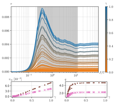
The operator average over a basis of P observables [cf. Eq. (3) of the main text] yields a statistically robust estimate of experimentally accessible -point correlation measurements of the external modes. To show this for the case , we replace the average in Eq. (3) by an average over all two-point density correlations
| (S1) |
where the operator counts the number of particles on site , irrespective of their internal states. Figure S1 shows for this average as a function of and of the particles’ indistinguishability, quantified by (as in Fig. 1 of the main text). We observe the same behavior as for the operator average, Eq. (3). The average (S1) shows a peak for (note a small shift to larger values in comparison to the operator average) followed by a decline to a plateau value . The dependence of and of the enhancement on is shown in the lower panels of Fig. S1 and compared to the results shown in the insets of Fig. 1. We observe, up to a scaling factor, exactly the same, strictly monotonic increase of both quantities with as in Fig. 1. To resolve this constant scaling factor between both averages, one needs to divide Eq. (3) by the dimensionality of the space of external two-particle observables. We omit this rather technical procedure here, since it is of no importance for our subsequent discussion.
.3 Schur-Weyl duality
Since dynamics and measurements are restricted to the external dof only, we trace out the internal dof. The reduced external system is conveniently described by the th tensor power of the external single-particle Hilbert space, . On this space, the symmetric and the unitary groups, and , act according to , , and , , respectively. Schur-Weyl duality states that these two group actions are dual to each other Fulton and Harris (2004). This implies that the external -particle space decomposes into a direct sum of irreducible representations of and , and , i.e.,
| (S2) |
The direct sum runs over Young diagrams (i.e., integer partitions of ), such as . While the reduced states of perfectly indistinguishable bosons only occupy the symmetric sector (which we therefore call the bosonic sector), , the reduced states of partially distinguishable particles typically occupy all sectors, as described in the main text.
Equation (S2) provides a convenient basis of , where and index basis states of the irreducible representations and , respectively. Each such basis state of and corresponds to a standard, respectively semi-standard Young tableau of shape Fulton and Harris (2004); Dufour et al. (2020). The number of standard and semi-standard Young tableaux, and , are combinatorial in nature and can be calculated via hook length formulas Fulton and Harris (2004). The table below lists them for the considered case of .
| 1 | 462 | |
| 5 | 1050 | |
| 9 | 1134 | |
| 10 | 840 | |
| 5 | 490 | |
| 16 | 896 | |
| 10 | 280 | |
| 5 | 175 | |
| 9 | 189 | |
| 5 | 35 | |
| 1 | 1 |
Adding up the dimensions with their corresponding multiplicities leads to the total dimension for the considered system. Note that the dynamics of the system is exclusively described by the irreducible representations of the unitary group, . Hence, the numbers of basis states of the irreducible representations of the symmetric group constitutes merely a multiplicity factor, and each symmetry sector decomposes into identical blocks of dimension . Since all blocks of one sector yield identical contributions to the dynamics, we can restrict the discussion to one of them for each sector, as done in Eq. (4).
An initial state with well-defined external occupation numbers occupies all Young basis states corresponding to semi-standard Young tableaux of shape compatible with the given occupation numbers. More precisely, these are exactly those Young tableaux that can be obtained by filling symbols ‘’ (for ) into the diagram by following the rules that each column must be strictly increasing and each row must be non-decreasing. The number of such tableaux for given occupation numbers is given by the so called Kostka-number Fulton and Harris (2004). In case of the homogeneous initial state () considered in Figs. 1 and 2 of the main text, semi-standard and standard Young diagrams are actually identical, leading to . In the limit , where the energy eigenstates approach the Young basis states, maximal localization is achieved with maximal inverse participation ratio , taking on a value larger than the inverse number of occupied Young basis states, i.e., (the populations on the occupied Young basis states are typically not uniform). This localization on a small number of energy states for , leads to a significant suppression of the numerator of [cf. Eq. (5)] in this limit. Note, moreover, that a lower tight bound of the purity for each sector is given by , which is achieved for perfectly distinguishable particles. Since , this implies maximal purity in the bosonic sector, independent of the particles’ distinguishability.
.4 Derivation of Eq. (4) of the main text
Under the assumption of a non-degenerate spectrum, the infinite time average of the time dependent expectation is given by
| (S3) |
with indicating the integration for . Definitions of are given in the main text. Integration over the exponential above yields . The second moment of the time signal is given by
| (S4) |
Assuming no degeneracies of levels and no gap-degeneracies between and within the -sectors, the time integration either decouples the sums over and or enforces a , leading to
| (S5) |
The first term is equal to the square of the time-averaged expectation , Eq. (S3). Subtracting this yields the variance
| (S6) |
Note that the variance is linear in , such that we can take the operator average over observables into the sum
| (S7) |
which is Eq. (4).
.5 Derivation of Eq. (5) of the main text
We show the factorization of into according to Eq. (4), under the considered statistical assumptions on the matrix elements and , namely that effectively occupies energy levels, that the observable is banded with bandwidth , and that the matrix elements of state and observable are statistically independent. For convenience, we define to be 1 on the eigenstates (indexed by ) closest in energy to the energy expectation of the considered homogeneous initial (Mott) state, and 0 elsewhere. Moreover let be 1 for and 0 for . With this we can calculate
with . The second equality exploits the statistical independence of the matrix elements of state and observable. The sums in line two run over a subset of indices of size . The sums in line three run over and indices, respectively. For this we correct by the introduced fractions in line three.
.6 Banded structure of the observable in the eigenstates
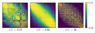
Figure S2 shows matrix plots of the operator averaged two-particle observable [cf. Eq. (3) of the main text] for three exemplary values of in the totally symmetric (bosonic) sector, for a system with . For small the observable does not yet develop a prominent band structure. However, in this parameter regime, the observable does not play a major role and the fluctuations [cf. Eq. (4) of the main text] are dominated by the strong localization of the initial state on only a small energy window. The clearest uniform band structure is observed for intermediate . For large , beyond the chaotic domain, a banded structure persists, however, the band is not uniformly occupied anymore.
.7 Contribution of the observable in Eq. (5) of the main text
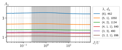
Figure S3 shows [cf. Eq. (5) in the main text] in the largest six symmetry sectors as a function of the control parameter . A system with is considered. As described in the main text, is almost constant as a function of , and of order of one in all shown sectors.
.8 Calculation of the averaged matrix elements of the observable
Here we derive the expression of in terms of the Hilbert-Schmidt inner products of particle-reduced energy eigenstates, as given in the footnote [68] of the main text (and implicitly also appearing in Eqs. (4) and (5)). The th tensor power of allows for a bipartition into the reduced P space and the remainder of the system. Let be an orthonormal basis of the operator space of Hermitian P operators which, together with the Hilbert-Schmidt inner product, forms a finite-dimensional Hilbert space of dimension . For pairs of eigenstates we define reduced operators , which for are just the P reduced density operators of the eigenstate Brunner (2019). For brevity we set and calculate
where the third equality uses the fact that the are an orthonormal basis. The proportionality factor accounts for the fact that the (implicit) extension of to the full P space is not normalized, more precisely Brunner (2019). The last equality can be shown using the Schmidt decomposition , which allows us to calculate