Deep learning in a bilateral brain with hemispheric specialization

Abstract

The brains of all bilaterally symmetric animals on Earth are divided into left and right hemispheres. The anatomy and functionality of the hemispheres have a large degree of overlap, but there are asymmetries and they specialize to possess different attributes. Several studies have used computational models to mimic hemispheric asymmetries with a focus on reproducing human data on semantic and visual processing tasks. In this study, we aimed to understand how dual hemispheres could interact in a given task. We propose a bilateral artificial neural network that imitates a lateralization observed in nature: that the left hemisphere specializes in specificity and the right in generalities. We used two ResNet-9 convolutional neural networks with different training objectives and tested it on an image classification task. Our analysis found that the hemispheres represent complementary features that are exploited by a network head which implements a type of weighted attention. The bilateral architecture outperformed a range of baselines of similar representational capacity that don’t exploit differential specialization. The results demonstrate the efficacy of bilateralism, contribute to an understanding of bilateralism in biological brains and the architecture serves as an inductive bias when designing new AI systems.

Impact statement A striking feature of the brain is that it is divided into two hemispheres. It is a conserved feature across all bilaterally symmetric animals, strongly suggesting its importance for intelligence. Many researchers have investigated observed hemispheric asymmetry. We take a different approach, assuming specialization, which enables an investigation into how dual hemispheres complement each other to improve performance. The study constitutes a novel approach to understanding the role of dual hemispheres for the cognitive sciences and the analysis provides possible mechanisms and testable predictions. In addition, the architecture outperformed a variety of comparable baselines, demonstrating that bilateralism is an important biologically-inspired principle to be considered in the design of new AI systems.

Keywords Hemispheric specialization, Hemispheric asymmetry, Brain-inspired architecture, Bilateral, Computational cognitive neuroscience, Deep learning, Inductive bias

1 Introduction

Many advances in the field of AI have been inspired by the human brain including the perceptron, reinforcement learning and imitation learning. Similarly, in this study, we took inspiration from the bilateral nature of the brain and applied it to a standard task likely to be affected by the bilateral architecture.

What is bilateralism?

The brain is divided into left and right hemispheres. It’s a remarkably conserved feature across species, suggesting its importance for intelligence. The anatomy and functionality of the hemispheres have a large degree of overlap, but they display an asymmetry and specialize to possess different attributes. One perspective is that the left hemisphere is specialized for specific classes and familiarity/routine whereas the right hemisphere is specialized for more general classes and novelty [1, 2, 3].

A likely explanation for the emergent specialization is small differences in functional and anatomical properties of the cortex. For example, the allocation of resources is organized differently within left and right hierarchies. The left resembles a pyramid with a greater density of neurons near input layers, whereas the right resembles an inverted pyramid, with greater neuron density near output layers [4, 5, 6, 1, 2, 3], see Fig. 1a. There is also a difference in network topology as a result of connectivity patterns. The left has more short local pathways constituting a modular network organization, whereas the right has more longer inter-regional pathways [1, 2, 3], see Fig. 1b. Important neurotransmitters such as dopamine and norepinephrine are asymmetrically distributed and the neuron firing thresholds differ between hemispheres [7]. In addition, the hemispheres respond asymmetrically to frequency, the left responds to higher frequencies than the right [8, 9, 10]. Asymmetry also arises through a split-fovea, where each hemisphere receives the contra-lateral half of the visual field [10, 11, 8, 12, 9, 13, 14]. Connectivity is also likely to play a major role in specialization and lateralized activity. Firstly with inter-hemispheric communication by the Corpus collosum (it is thought to result in a competitive process between the hemispheres) [5, 4, 7, 12] and intra-hemispheric with different patterns of connectivity between regions within each hemisphere [15, 16]. Finally, there may be additional substrate differences that are not yet discovered.

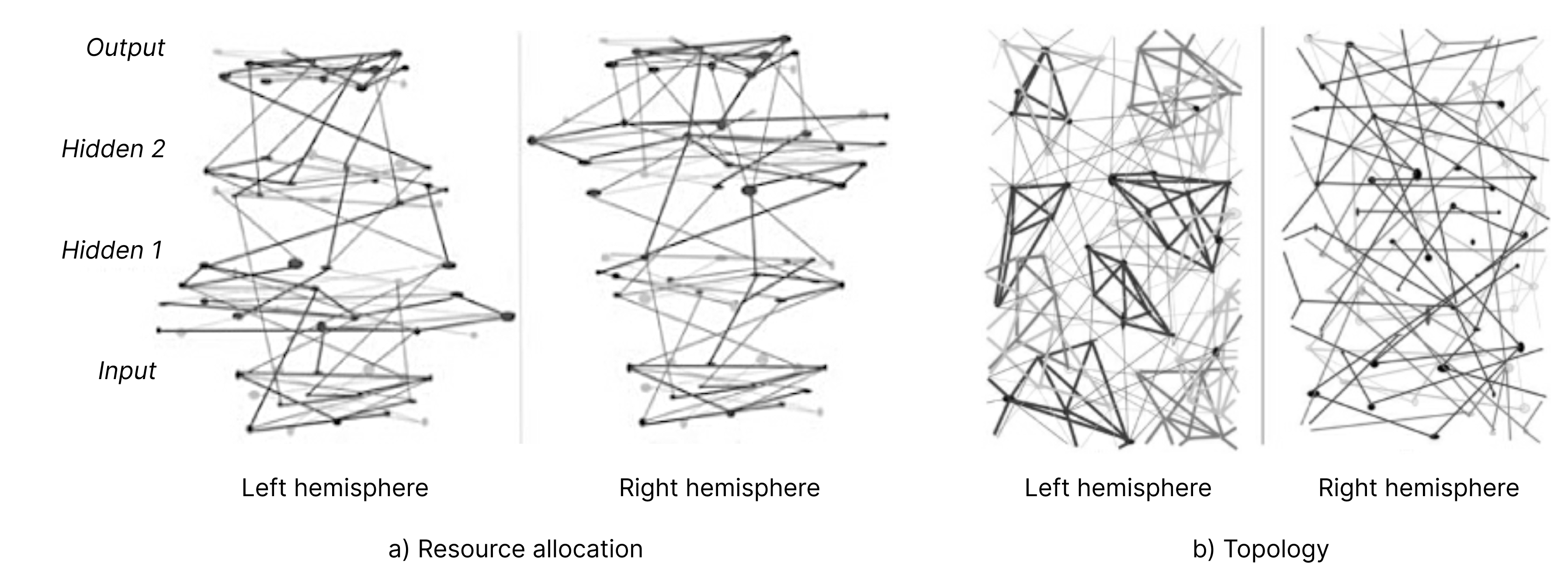
Figure 1: Hemispheric differences a) Resource allocation: the left is pyramidal, the right is an inverted pyramid, and b) Topology: the left has shorter more local pathways and the right has longer more distant pathways. From Elkhonon Goldberg, The New Executive Brain, Oxford University Press, 2009, Fig 6.2, p. 70; Fig. 14.1, p. 263. Reproduced with permission of Oxford University Press

Many researchers have used computational models to study the bilateral brain. They mimic anatomical and functional asymmetries, subject the system to standard tasks, and compare the results to human behavioral data. See ‘Related Work’, Section 2. The various studies provide evidence that asymmetric functional and anatomical differences can give rise to observed lateralization of activity for specific tasks. An important question is not usually addressed directly - what is the benefit of having dual hemispheres and how do they complement each other? The aim of this project is to investigate the representations in each hemisphere and how that makes the total system better at a given task.

1.1 Our approach

We investigated bilateralism through a computational model, with the objective of developing a theory of operation and to understand how bilateral principles could be exploited for AI/ML. As a starting point, we focused on the left hemisphere’s specialization on specifics, and the right’s specialization on generalities. We assume the testable hypothesis that an ANN with differentially specialized sub-networks would outperform a single comparable network in a classification task featuring both general and specific classes.

We chose a hierarchical image classification task where each sample belongs to both a general and a specific class. For example, general: sea creature, specific: penguin, seal, shark etc. We modeled the hemispheres with left and right artificial neural networks, specialized through supervised training on general or specific classes. The bilateral network was compared to several comparative baselines that do not have specialization and the differences were analyzed, to explore the effects of bilateral specialization.

The source code is available at [17].

2 Related Work

2.1 Hemispheric asymmetry

In the field of cognitive neuroscience, there are multiple studies that examine hemispheric function in standard behavioral tasks. The studies use bilateral artificial neural networks with asymmetries that mimic functional and anatomical properties of the cortex and replicate aspects of human behavioral data on the tasks, including lateralized hemispheric activity. Some of the studies also consider neurological development, disorders or damage and recovery. With the exception of face perception studies, they all used synthetic abstracted representations for input and output vectors and do not operate on realistic sensory data.

The behavioral tasks can be divided into two major groups, semantic processing and visual perception. The work is summarized below and organized visually in a taxonomy in Figure 2.

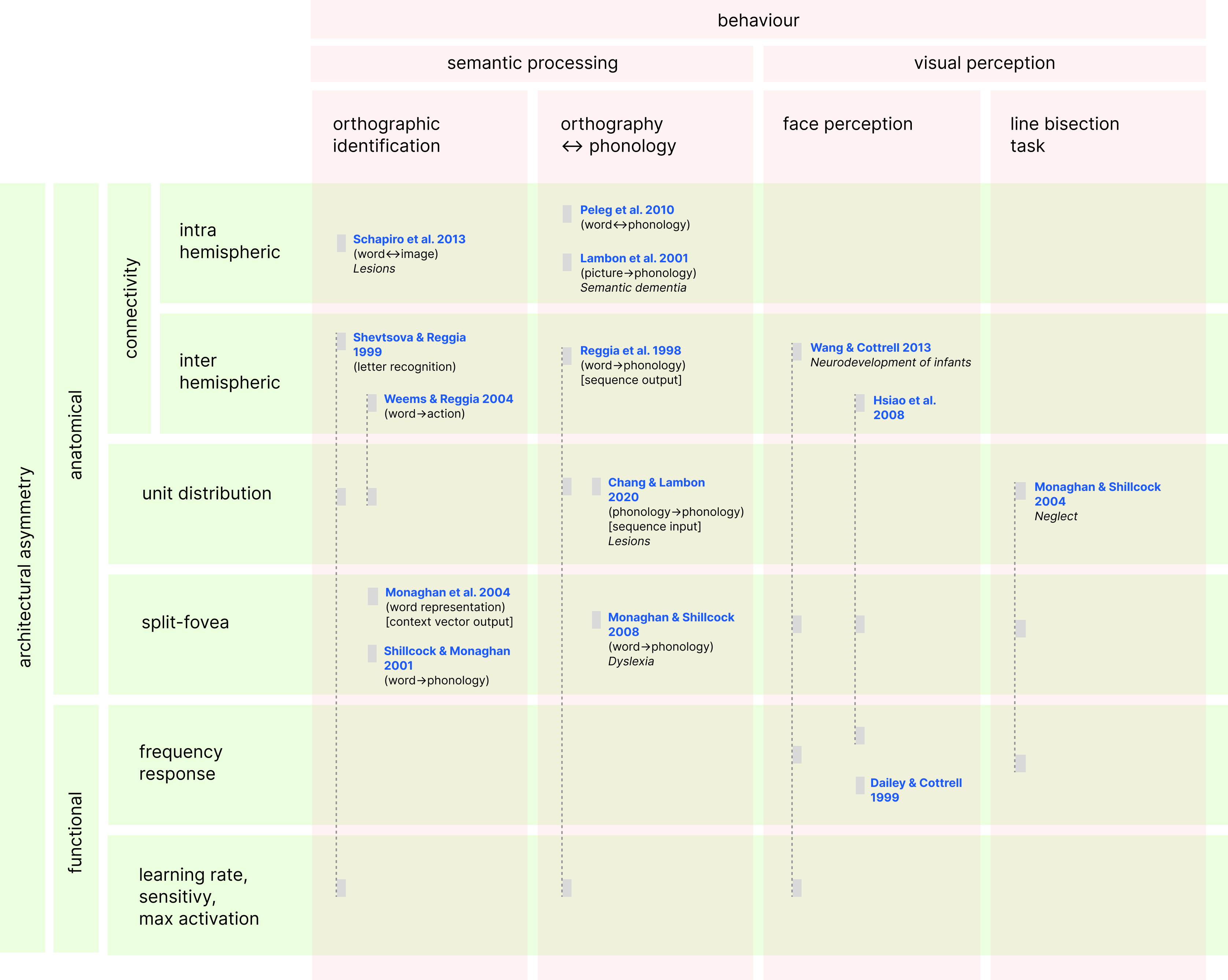
Figure 2: A taxonomy of bilateral computational models: The literature is organized according to two overlapping taxonomies, driven by a) architectural asymmetry and b) behavior. The text in parentheses provides more detail on the type of behavioral experiment conducted. Where it is not possible to deduce the experimental equivalent of the behavioral task, the text in square parentheses provides more detail. If a disorder was investigated, this is shown in italicized text.

For semantic processing, behavioral data and patterns of hemispheric asymmetry were reproduced by varying intra-hemispheric connectivity [16] in the context of semantic dementia [18], and in the context of unilateral and bilateral lesions [15]. Other studies varied anatomical features such as inter-hemispheric connectivity and the distribution of units between layers, as well as functional features such as learning rate, sensitivity and maximum unit activation and combinations of these factors [5, 4, 7] and in the context of lesions and recovery [6]. Another anatomical feature that was explored is the split-fovea by Monaghan et al. [10] and in the context of dyslexia by Monaghan and Shillcock [11]. Hemispheric asymmetry emerged as a result of the orthographic to semantic patterns inherent in the language.

Visual perception tasks can be further divided into face perception and the line-bisection task. Face perception includes identification of faces and emotions. In the line-bisection tasks, subjects are asked to mark the center of a horizontal line. Perception of the center is affected by hemispheric function. Face perception was first studied by Dailey and Cottrell [9] with a model that mimicked the hemispheric frequency response asymmetry. Hsiao et al. [8] added a split-fovea and then Wang and Cottrell [12] incorporated other functional parameter differences between the hemispheres as well as a learned gating mechanism for inter-hemispheric communication. For the line bisection task, Shillcock and Monaghan [13] and Monaghan and Shillcock [14] used a split-fovea, asymmetric frequency response as well as asymmetric distribution of units in layers between left and right.

In the closest work to this project, Mayan et al. [19] tackled the same problem of image classification with specific and general (hierarchical) classes. The authors created a single network with two hemispheres, and trained it with supervised learning and a single loss function. They used hyperparameters with analogies to biological parameters in each hemisphere to encourage specialization. Specialization was achieved in each side but the bilateral network did not have an advantage over baselines.

2.2 Biologically inspired multi-network architectures

Several studies cover related ideas, although they did not explicitly model bilateral hemispheres. Beaulieu et al. [20] created a dual-stream architecture called Neuromodulator Meta-learner, where one network learns to modulate the other, to enhance continual learning. Bakhtiari et al. [21] created a network with parallel pathways to reproduce the functionality of dorsal (‘where’) and ventral (‘what’) pathways in an ANN trained with a single loss function. Li and Deza [22] discussed specialization of a branched neural network when trained on a Gabor filter dataset and found that the training curriculum is inconsequential to specialization of the branched neural network.

2.3 Ensemble model

The dual-hemisphere architecture in this work can be viewed as an ensemble model. Ensembling is a popular approach in ML [23]. The most common techniques involve combining the outputs of the same model type, trained with different seeds. However, there are also many techniques that encourage diversity within the ensemble using different training objectives, sampling, architecture, or losses [24, 25, 26]. Our work may be seen as a special case of a diversified ensemble, where the ensemble architecture exploits hierarchical data labels to achieve the diversification.

2.4 Hierarchical image datasets

We focused on image classification of specific and general classes, exploiting the hierarchical nature of CIFAR-100 [27]. CIFAR-100 and other hierarchical image classification datasets are widely used as benchmarks, including ImageNet [28] and Omniglot [29]. However, the hierarchical nature of available classes is rarely exploited to enhance training or generate a more difficult task. Notable exceptions arise in the Continual Few-Shot Learning literature, such as the Meta-Dataset of Triantafillou et al. [30] which generates class-hierarchy-aware episodes of data and the Tiered-ImageNet of Caccia et al. [31] which uses class hierarchy to generate Out of Distribution (OoD) data.

3 Model

We implemented the bilateral architecture as well as several baselines, described in the subsections below.

3.1 Bilateral network

We predicted that with specialization, the hemispheres would extract distinct but overlapping features, despite identical observations. In addition, we expected that a bilateral architecture would be able to combine these features to improve overall accuracy.

We used ResNet-9 [32] as the base convolutional vision architecture for the individual hemispheres. This architecture was chosen for its combination of simplicity and relatively good performance in image classification tasks. ResNet-9, shown in Fig. 3, has 9 layers and skip connections that help to overcome vanishing gradients.

The number of layers was optimized empirically on the selected dataset. To introduce specialization, the left hemisphere was trained on specific classes and the right hemisphere on general classes.

We created the bilateral architecture by concatenating the output of the penultimate layers of each hemisphere and adding 2 heads, one for specific and one for general classes, see Fig. 4. The heads consist of a single fully-connected layer and a softmax layer. After training the individual hemispheres, their weights were frozen to prevent any further changes, and the heads were then trained.

A detailed description of the training and evaluation is given in the experimental method, Section 4.1.

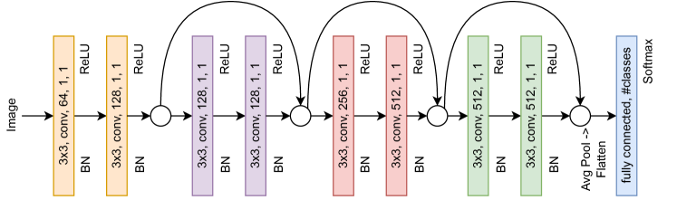
Figure 3: ResNet-9 architecture: A convolutional neural net with 9 layers and skip connections.

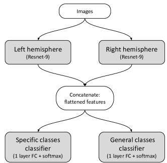
Figure 4: Bilateral architecture: The feature vectors from the left and the right hemispheres are concatenated and fed to the heads to classify specific and general classes respectively.

3.2 Baseline models

Bilateral network without specialization

To better understand the role of specialization, we compared the bilateral model to an equivalent network without specialization. We trained the entire network (two hemispheres and heads) without first explicitly inducing specialization in the individual hemispheres.

Unicameral network

Two hemispheres have more resources (in terms of trainable parameters) than one of those hemispheres. To better understand the impact of increasing the available resources, we compared the bilateral model to different sized unicameral architectures. Like the bilateral network, there are two heads on the penultimate layer, one for specific and one for general classes. We used the predefined 18-layered and 34-layered ResNet architectures. The 18-layered network has approximately the same number of trainable parameters as the bilateral network, and the 34-layered network approximately double.

Ensembles

The bilateral network is a type of ensemble. Ensemble learning denotes combining different models or algorithms to obtain improved performance over a single model [23]. To understand the differences between differential specialization and conventional ensembling, we compared to two different models, one was a 2-model ensemble and one was a 5-model ensemble. In order to construct the ensembles, we used a common approach where we trained 10 unicameral ResNet-9 models, and selected the top-$k$ ($k$ was 2 and 5 respectively). The output of the ensemble in training and inference was the mean output from the models.

4 Experiments

4.1 Experimental setup

Dataset

We used the CIFAR-100 dataset [27], as it includes hierarchical labels that denote generic and specific classes.

Training and evaluation

Training and evaluation was repeated over 100 epochs and from 5 random seeds. All training was supervised with a cross-entropy loss function. We utilized two widely used data augmentation techniques, RandomCrop and RandomHorizontalFlip. We used weight decay and dropout [33] to regularize the models and Adam [34] for optimization. The images were resized to 32x32, with a learning rate of 1.0e-3, batch size of 512, and weight decay of 1.0e-4. We used a ReLU non-linearity in all networks.

Evaluation was carried out with a disjoint test set, in the multilabel classification setting. The image resolution was 32x32 and there was no test data augmentation.

Framework and computational resources

Experiments were conducted with the PyTorch-Lightning [35] research framework, a wrapper around the PyTorch library [36]. All models were trained and evaluated on a single NVIDIA RTX 3060.

4.2 Visualizing network operation

We used two types of visualizations to better understand the operation of the bilateral network.

Gradient camera (Grad-Cam) visualization

The bilateral network and individual hemispheres utilize encoded features from the convolutional layers to predict a class label. To understand how the extracted features contribute to classification, we visualized the gradient flow [37, 38, 39] averaged over convolutional layers while the model predicted a class, using the Grad-Cam library. The gradient heatmap highlights the region of focus for both hemispheres and the overall network (average over both heads).

Feature analysis using cosine similarity

We investigated how left and right features are exploited by the bilateral network by analyzing the relationship between representations in different parts of the network, with a focus on how the representations are transformed by the network heads. We did this by measuring the similarity of features for images of the same label. They are expected to have similar features, so measuring the feature similarity at different parts of the network should be revealing.

We first grouped the image samples into random pairs with the same class label. We then plotted a bivariate distribution of cosine similarity between the pairs, one for the input to the heads, denoted ‘concatenated’ and the other for the average of the network head outputs, denoted ‘bilateral’. The distributions plot similarity along the following dimensions: left hemisphere, right hemisphere and a third dimension, either concatenated or bilateral. Additionally, univariate marginal distributions were plotted for each hemisphere.

5 Results

5.1 Accuracy

Quantitative results are summarized in Fig. 5 and Table 1. The bilateral model with specialization provided a boost of almost 10% in both general and specific classes over the individual specialized hemisphere. The bilateral model with specialization outperformed all of the baselines, except for the 5 model ensemble, which had comparable performance but significantly more trainable parameters.

Model	# Params	General class Accuracy	Specific class Accuracy
Left hemisphere	6.62 M	—	63.84 $\pm$ 0.95%
Right hemisphere	6.58 M	73.64 $\pm$ 2.5%	—
Bilateral neural network   with specialization	13.33 M	81.55 $\pm$ 0.03%	72.14 $\pm$ 0.17%
Bilateral neural network      without specialization	13.33 M	75.60 $\pm$ 1.13%	65.21 $\pm$ 1.17%
Unicameral - ResNet-18	11.24 M	75.60 $\pm$ 0.58%	64.98 $\pm$ 0.68%
Unicameral - ResNet-34	21.35 M	76.80 $\pm$ 0.23%	65.53 $\pm$ 0.81%
Ensemble of 2 ResNet-9’s	13.3 M	79.50 $\pm$ 0.45%	70.50 $\pm$ 0.95%
Ensemble of 5 ResNet-9’s	33.25 M	81.40 $\pm$ 1.05%	73.40 $\pm$ 0.85%

Table 1: Accuracy of models

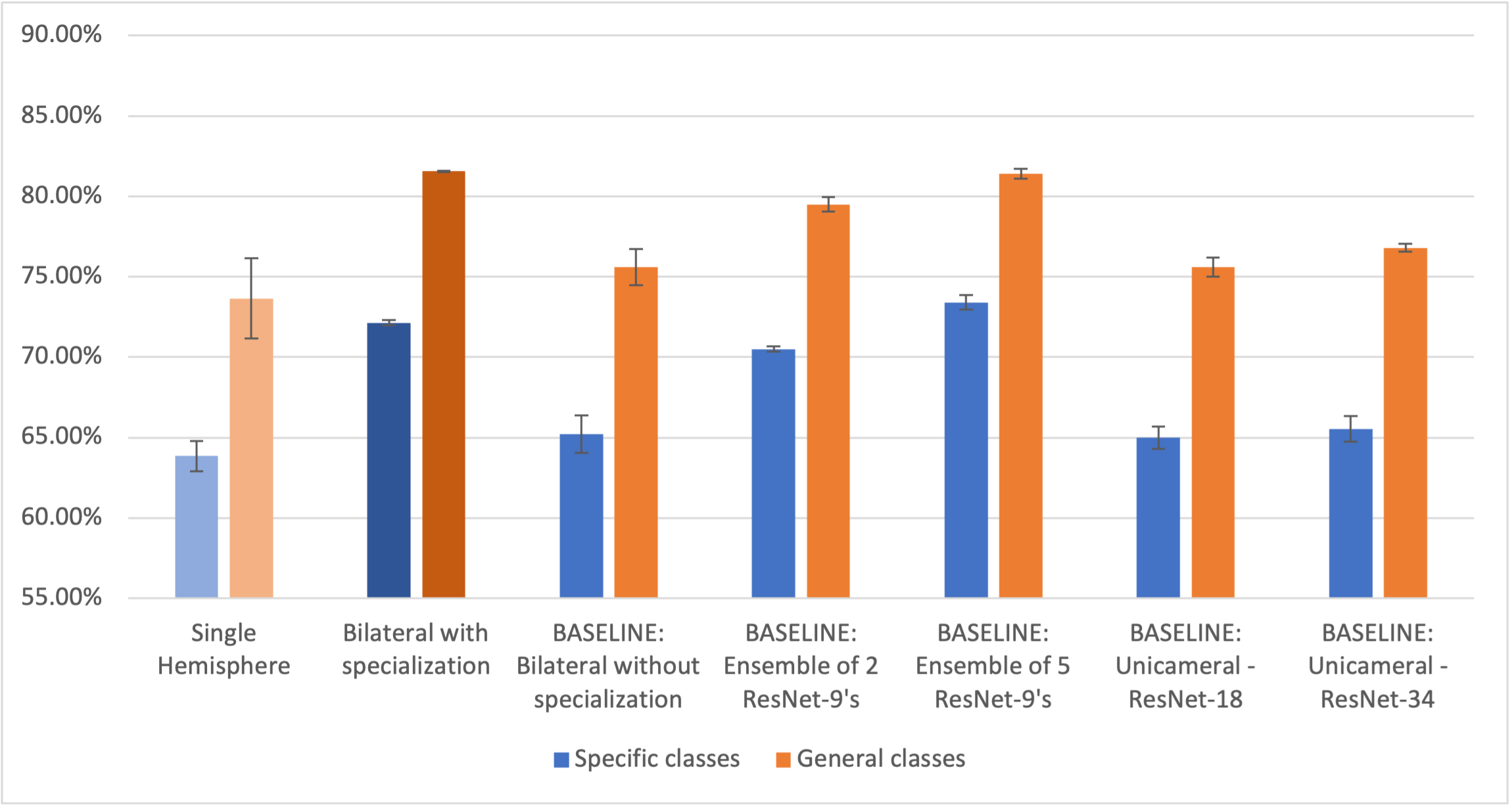
Figure 5: Accuracy of models

5.2 Visualizing network operation

Visualizations of Grad-Cam and similarity distributions are shown for selected scenarios. In order to be informative, we selected key scenarios that are distinct from each other and highlight the contribution of different parts of the network. The scenarios are:

• Scenario 1: The bilateral network is correct, left and right hemispheres are incorrect.

• Scenario 2: The bilateral network and the right hemisphere are correct, the left hemisphere is incorrect.

• Scenario 3: The bilateral network and the left hemisphere are correct, the right hemisphere is incorrect.

• Scenario 4: The bilateral network is incorrect, the left and right hemispheres are correct.

The definition of ‘correct’ for the bilateral network, is that it was successful for both specific and general class labels.

The Grad-Cam visualizations are shown in Figures 6 to  9. In general, the features are more local in the left hemisphere and more global in the right hemisphere. The heads blend different aspects of features from the left and right hemispheres for the task. The effect is that in many cases, features trained for specific classes are helpful for general classes and vice versa, and a correct classification can be achieved even if both hemispheres are individually incorrect.

(a) Bosc Image

(b) Left hemisphere

(c) Right hemisphere

(d) Bilateral ANN

Figure 6: Grad-Cam for Scenario 1: The bilateral network is correct, left and right hemispheres are incorrect. The bilateral network adjusts the area of focus even when both the hemispheres’ features are situated well external to the bosc.

(a) Tank Image

(b) Left hemisphere

(c) Right hemisphere

(d) Bilateral ANN

Figure 7: Grad-Cam for Scenario 2: The bilateral network and the right hemisphere are correct, the left hemisphere is incorrect. Since there are multiple labels with wheels, the left failed to differentiate the tank by its wheels alone, however the bilateral appears to overcome this, using the right hemisphere’s features.

(a) Cycle Image

(b) Left hemisphere

(c) Right hemisphere

(d) Bilateral ANN

Figure 8: Grad-Cam for Scenario 3: The bilateral network and the left hemisphere are correct, the right hemisphere is incorrect. The left hemisphere identifies more local features of the bicycle compared to the right. The network heads make the necessary adaptations to give an accurate prediction.

(a) Sofa Image

(b) Left hemisphere

(c) Right hemisphere

(d) Bilateral ANN

Figure 9: Grad-Cam for Scenario 4: The bilateral network is incorrect, the left and right hemispheres are correct. Both hemispheres identify local and global features. The network heads over-compensate and focus on the region outside of the sofa.

The cosine similarity results are shown in Fig. 10 and Fig.11. In the concatenated distribution, there is a strong correlation between similarity in left and concatenated, and right and concatenated. In contrast, there is no obvious correlation in the bilateral distribution. The network heads learned a non-linear transformation of the feature space.

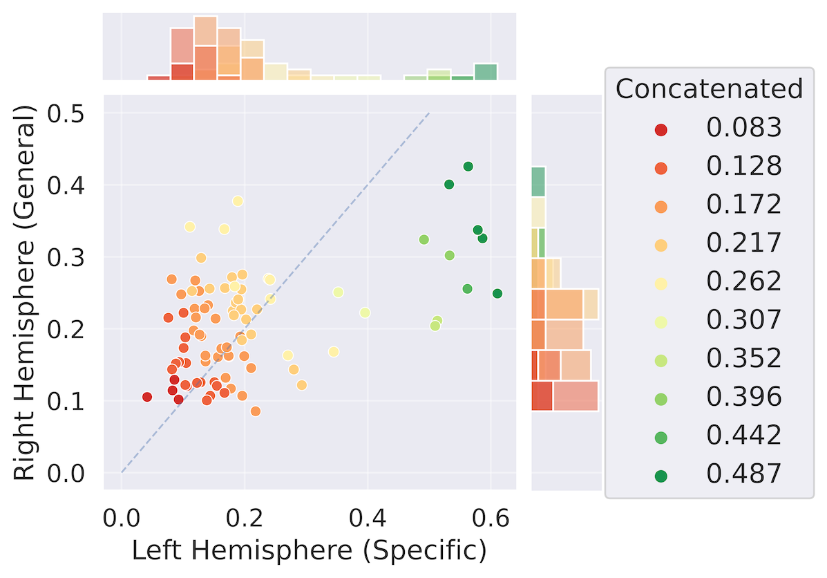
(a) Concatenated

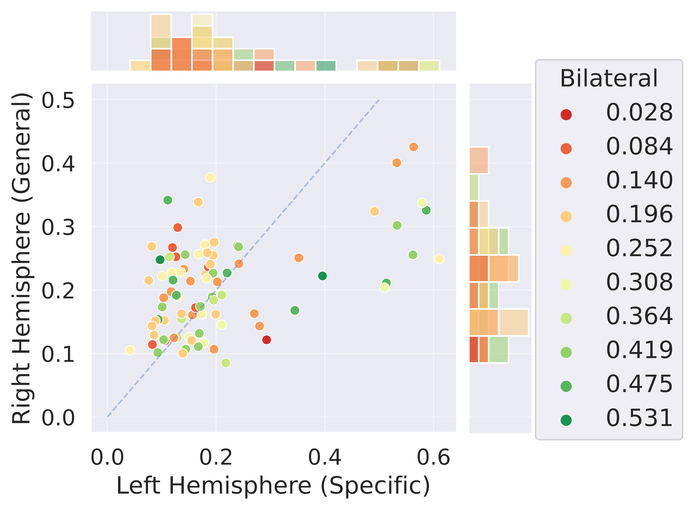
(b) Bilateral network

Figure 10: Cosine similarity distribution for Scenario 1: The bilateral network is correct, left and right hemispheres are incorrect. Many of the pairs (same label) have dissimilar (values closer to 0) features in left and right, seen in the density of points close to the origin. The concatentated features are also dissimilar, but the bilateral network elevates the similarity of many of the points. Each point is a pair of images with the same label. The x-axis is similarity in the left hemisphere, y-axis is similarity in the right hemisphere. The color is similarity in the combined representation. Additionally, the univariate marginal distributions are shown for left and right with histograms above and to the side of the bivariate distribution.

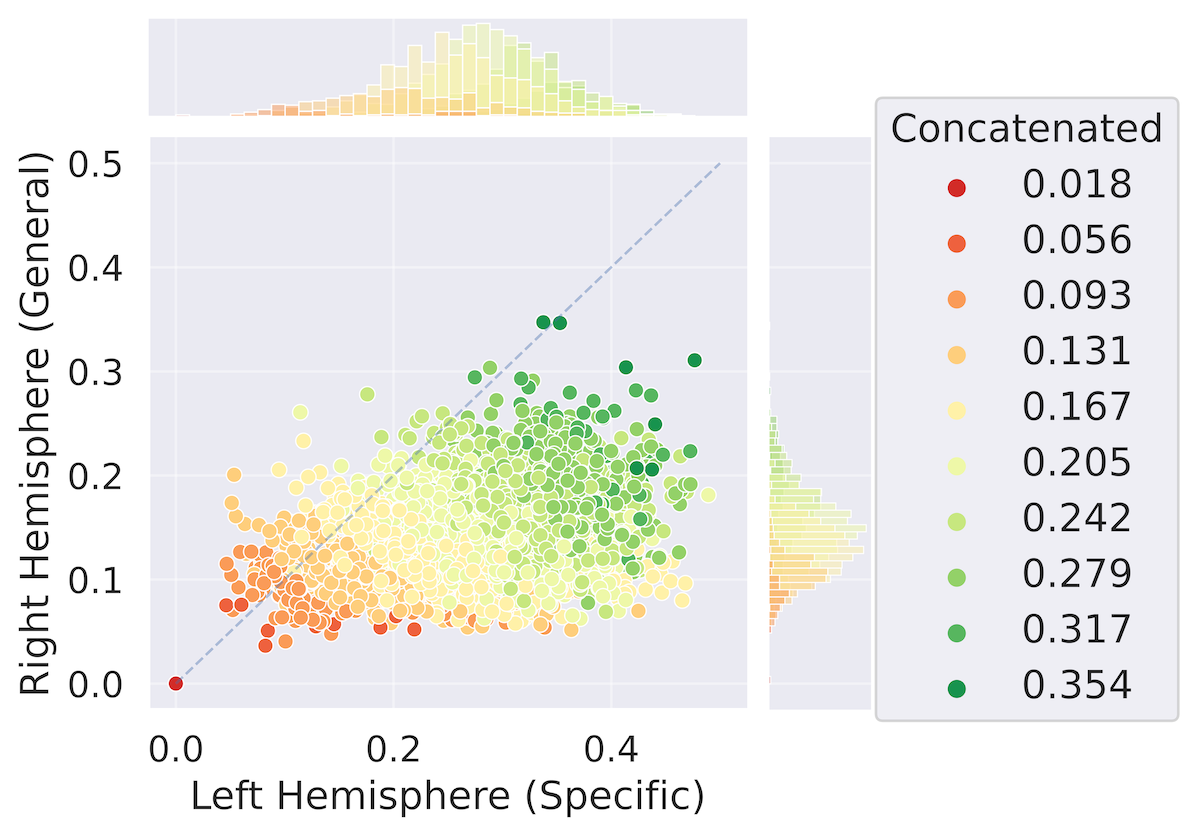
(a) Concatenated

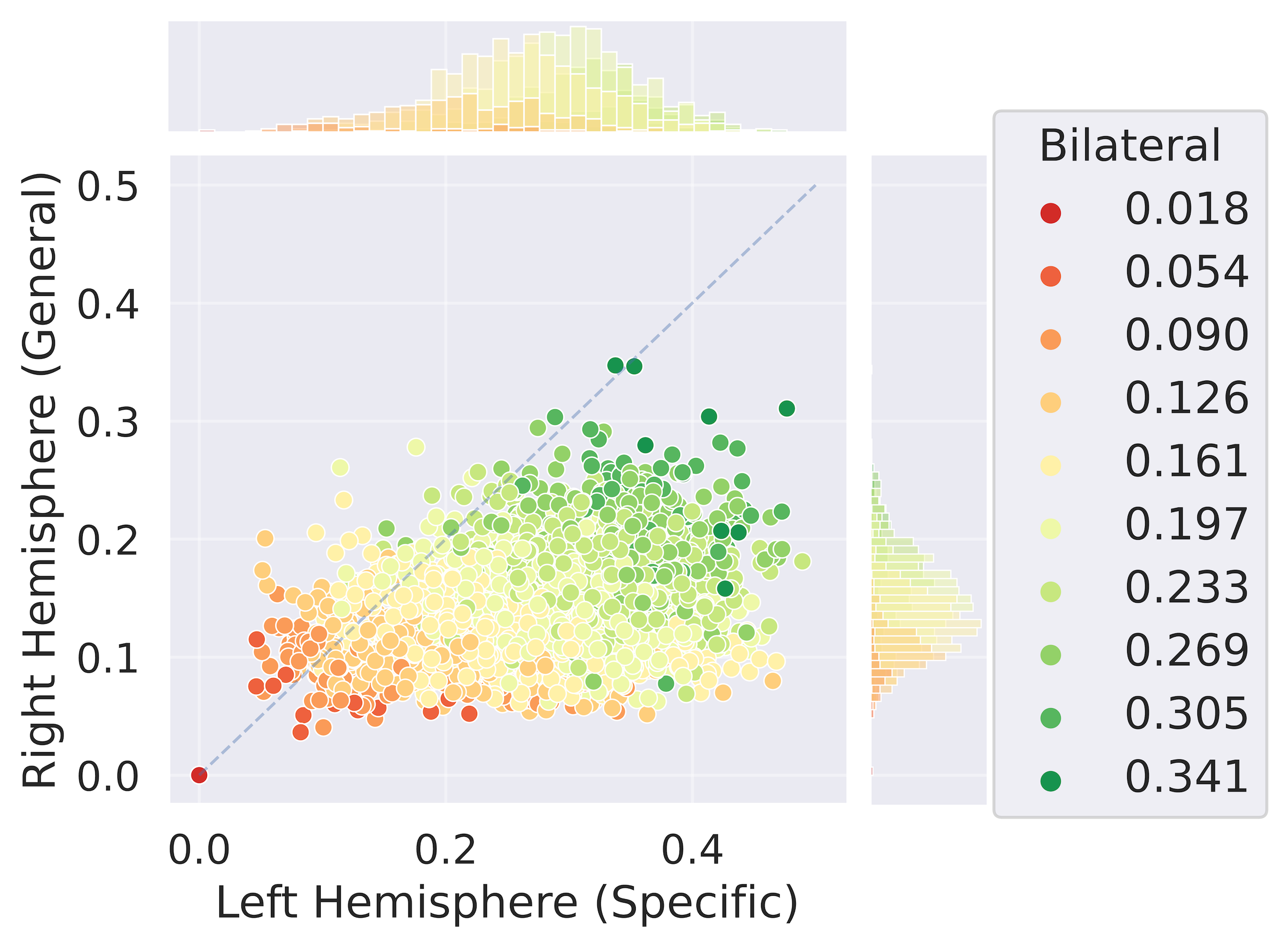
(b) Bilateral network

Figure 11: Cosine similarity distribution for Scenario 2: The bilateral network and the right hemisphere are correct, the left hemisphere is incorrect. Some regions with points that have low similarity in the left (at approximately x, y = 0.2, 0.2), have elevated similarity in the bilateral output, compared to concatenated. Also, for points with high similarity in the left (approximately 0.35, 0.1), the similarity is lower in the bilateral output. In other words, the bilateral network was able to exploit features in the right hemisphere over the left. Each point is a pair of images with the same label. The x-axis is similarity in the left hemisphere, y-axis is similarity in the right hemisphere. The color is similarity in the combined representation. Additionally, the univariate marginal distributions are shown for left and right with histograms above and to the side of the bivariate distribution.

6 Discussion

6.1 Key findings

We conducted experiments to implement and study bilateralism in an Artificial Neural Network. The effects of bilateralism were studied by comparing against baselines that captured distinct characteristics of the proposed bilateral network. We used a classification task with hierarchical classes that captured an observed characteristic of biological hemispheres, that the left is more specialized for specific classes and the right for general classes. The results confirmed the hypothesis that a bilateral architecture with differential specialization in left and right hemispheres confers an advantage over conventional architectures on this multilabel hierarchical classification task.

More specifically, we found that there is an advantage of two hemispheres over one network, demonstrated by the fact that the bilateral architecture outperformed a) individual hemispheres and b) unicameral networks with the same and double the number of trainable parameters. The latter case shows that the advantage was not simply due to a higher number of trainable parameters. Furthermore, we found that having two hemispheres is not sufficient, but that specialization is important, shown by the benefit of the bilateral ANN with specialization over the bilateral ANN without. Finally, we found that the advantage of the bilateral network does not arise from the fact that it is an ensemble, shown by the result that the 2 model ensemble was less effective, and it took a 5 model ensemble without explicit specialization to reach the same level of performance.

6.2 Why does a bicameral architecture help?

The Grad-Cam images reveal that the left hemisphere extracts more localized features than the right. Different learning objectives enable them to capture different aspects of the environment. Collectively the set of features is greater than one network with one objective.

Interestingly, even though the left is explicitly trained on specific class labels, the features that it extracts are helpful for general classes. The inverse is true of the right.

With reference to the cosine similarity visualization, before the network heads, the similarity of pairs of images of the same class is correlated with left and right. The similarity is no longer correlated after the network heads, which must implement some sort of non-linear transformation. In many cases, when left or right produce ineffective features, shown by low similarity between these images of the same class, the heads are able to produce features that have increased similarity. The network heads learn to combine the features from left and right, to different degrees, to produce better predictions. In some cases, the bilateral network makes a correct classification, even if both hemispheres are individually wrong.

In summary, specialization creates a higher diversity of features. The network heads implement a type of weighted attention to left and right hemispheres selectively in a task dependent manner, improving overall class prediction.

6.3 Relation to biology

A limitation of our model, in terms of biological accuracy, was that inter-hemispheric connectivity was achieved at the outputs of the hemispheres. In contrast, biological hemispheres are interconnected throughout their hierarchies [40]. Nevertheless, the heads may serve a similar purpose, albeit in a cruder way. Inter-hemispheric connectivity comprises a complex combination of inhibitory and excitatory projections. The hemisphere that is better able to represent the input is likely to have stronger activation and thus inhibit the other hemisphere [4, 5]. Like the heads, this too is a type of selectivity. Building a model with interconnected hemispheres throughout the hierarchy is a topic for future research.

The central finding that in our model, left and right hemispheres extracted local and non-local features, used together in specific tasks, provides one plausible suggestion for the prevalence of bilateral brains in nature and is a testable prediction for biological brains. A possible approach to test the prediction is with transcranial magnetic stimulation (TMS) to selectively impair one hemisphere at a time on controlled tasks [41].

6.4 Why it’s important

The key findings are a small step towards understanding and taking advantage of the characteristics of biological brains, and show the potential of bilateralism to improve ML/AI. More broadly, it’s a biological principle that warrants further investigation.

The fact that bilateralism has a material effect on the network as a whole, suggests that bilateralism should be considered for other cognitive neuroscience models, where it is usually ignored. One potentially fruitful area is extending the standard Hippocampal/Neocortical model, CLS [42, 43], by introducing asymmetries into the bilateral Hippocampal architecture. Indeed, evidence exists of asymmetric contributions of left and right Hippocampi to memory [44, 45].

Bilateralism could also inspire new priors or inductive biases to improve ML models.

6.5 Future work

A promising direction to improve the model as well as our understanding of the neuroscience, is to further investigate and model the neurobiology. There are several avenues. For example, replicating recurrent connectivity, more complex biologically inspired interactions between the hemispheres, mimicking known substrate differences between the hemispheres such as topological differences, resource allocation (see Fig. 1) and experiments on inducing specialization without supervision.

This study focused on one aspect of bilateralism with an image classification task. There are also interesting lateral effects for motor control. For example, in most people, the right hand is better at trajectories, and the left hand is better at position/posture (dynamic dominance theory [46]). Developing an architecture and experiments to explore motor control is an interesting area for future work.

One theory is that the observed differences between the hemispheres emerge from a more fundamental specialization for novelty (right) and routine (left) [1, 2, 47]. These ideas could be explored with an agent that can act in a dynamic environment. The right hemisphere could be a generalist that can perform unfamiliar tasks as a beginner, while the left becomes an expert over time. The agent would be able to adopt new tasks, without being inept at them. Currently, the field of Continual RL does not focus on avoiding poor performance, but rather maximizing the best performance. In real-life scenarios however, an agent must avoid death and serious injury to themselves and those around them (also relevant for physical robots and virtual artificial agents).

As mentioned earlier in this section, bilateralism could be incorporated into existing cognitive computational models, and the benefits of bilateralism could be studied within more powerful ML architectures.

7 Conclusion

We built a bilateral architecture with left and right neural networks, inspired by our bilateral brains. The hemispheres were trained to specialize on specific and general classes. They extracted specialized features and through a type of ‘weighted attention’ by a simple fully connected layer, outperformed various baselines on classification of both specific and general class labels. The specialized representations had benefits above the explicit objective of their individual hemisphere. The results demonstrate that small procedural changes to training can achieve specialization, and that specialization can be complementary and beneficial for certain tasks. The operation of the artificial network provides testable hypotheses regarding neurobiological hemispheric specialization. Simultaneously, this work shows that neuroscientific principles can provide inductive biases for novel ML architectures. Currently, in the field of AI/ML where scaling of existing architectures is achieving great success, it’s interesting to look at new principles on smaller architecture that could then be scaled.

Author contributions

GK conceived and supervised the project, CR designed and implemented the experiments, GK and CR authored the manuscript, DR advised and assisted with the manuscript and EG introduced the concept and provided advice. All authors read and approved the final manuscript.

References

- Goldberg and Costa [1981] Elkhonon Goldberg and Louis D Costa. Hemisphere differences in the acquisition and use of descriptive systems. Brain and Language, 14:144–173, 1981. ISSN 0093-934X. doi:https://doi.org/10.1016/0093-934X(81)90072-9. URL https://www.sciencedirect.com/science/article/pii/0093934X81900729.
- Goldberg et al. [1994] E. Goldberg, K. Podell, and M. Lovell. Lateralization of frontal lobe functions and cognitive novelty. Journal of Neuropsychiatry and Clinical Neurosciences, 6:371–378, 1994. ISSN 08950172. doi:10.1176/JNP.6.4.371. URL /record/1995-12594-001.
- Goldberg et al. [2013] Elkhonon Goldberg, Donovan Roediger, N Erkut Kucukboyaci, Chad Carlson, Orrin Devinsky, Ruben Kuzniecky, Eric Halgren, and Thomas Thesen. Hemispheric asymmetries of cortical volume in the human brain. Cortex, 49:200–210, 2013. ISSN 00109452. doi:10.1016/j.cortex.2011.11.002. URL http://dx.doi.org/10.1016/j.cortex.2011.11.002.
- Shevtsova and Reggia [1999] Natalia Shevtsova and James A. Reggia. A neural network model of lateralization during letter identification. Journal of Cognitive Neuroscience, 11:167–181, 1999. ISSN 0898929X. doi:10.1162/089892999563300. URL /record/1999-05033-003.
- Weems and Reggia [2004] Scott A. Weems and James A. Reggia. Hemispheric specialization and independence for word recognition: A comparison of three computational models. Brain and Language, 89:554–568, 6 2004. ISSN 0093-934X. doi:10.1016/J.BANDL.2004.02.001.
- Chang and Ralph [2020] Ya Ning Chang and Matthew A. Lambon Ralph. A unified neurocomputational bilateral model of spoken language production in healthy participants and recovery in poststroke aphasia. Proceedings of the National Academy of Sciences of the United States of America, 117:32779–32790, 12 2020. ISSN 10916490. doi:10.1073/PNAS.2010193117/SUPPL_FILE/PNAS.2010193117.SAPP.PDF. URL https://www.pnas.org/doi/abs/10.1073/pnas.2010193117.
- Reggia et al. [1998] James A. Reggia, Sharon Goodall, and Yuri Shkuro. Computational studies of lateralization of phoneme sequence generation. Neural Computation, 10:1277–1297, 7 1998. ISSN 0899-7667. doi:10.1162/089976698300017458. URL https://direct.mit.edu/neco/article/10/5/1277/6196/Computational-Studies-of-Lateralization-of-Phoneme.
- Hsiao et al. [2008] Janet Hui Wen Hsiao, Danke X. Shieh, and Garrison W. Cottrell. Convergence of the visual field split: Hemispheric modeling of face and object recognition. Journal of Cognitive Neuroscience, 20:2298–2307, 12 2008. ISSN 0898929X. doi:10.1162/JOCN.2008.20162.
- Dailey and Cottrell [1999] M. N. Dailey and G. W. Cottrell. Organization of face and object recognition in modular neural network models. Neural Networks, 12:1053–1074, 10 1999. ISSN 0893-6080. doi:10.1016/S0893-6080(99)00050-7.
- Monaghan et al. [2004] Padraic Monaghan, Richard Shillcock, and Scott McDonald. Hemispheric asymmetries in the split-fovea model of semantic processing. Brain and Language, 88:339–354, 3 2004. ISSN 0093-934X. doi:10.1016/S0093-934X(03)00165-2.
- Monaghan and Shillcock [2008] Padraic Monaghan and Richard Shillcock. Hemispheric dissociation and dyslexia in a computational model of reading. Brain and Language, 107:185–193, 12 2008. ISSN 0093-934X. doi:10.1016/J.BANDL.2007.12.005.
- Wang and Cottrell [2013] Panqu Wang and Garrison Cottrell. A computational model of the development of hemispheric asymmetry of face processing. Proceedings of the Annual Meeting of the Cognitive Science Society, 35:35, 2013. ISSN 1069-7977.
- Shillcock and Monaghan [2001] Richard Shillcock and Padraic Monaghan. The computational exploration of visual word recognition in a split model. Neural Computation, 13:1171–1198, 5 2001. ISSN 08997667. doi:10.1162/08997660151134370.
- Monaghan and Shillcock [2004] Padraic Monaghan and Richard Shillcock. Hemispheric asymmetries in cognitive modeling: connectionist modeling of unilateral visual neglect. Psychological review, 111:283–308, 4 2004. ISSN 0033-295X. doi:10.1037/0033-295X.111.2.283. URL https://pubmed.ncbi.nlm.nih.gov/15065911/.
- Schapiro et al. [2013] Anna C. Schapiro, James L. McClelland, Stephen R. Welbourne, Timothy T. Rogers, and Matthew A.Lambon Ralph. Why bilateral damage is worse than unilateral damage to the brain. Journal of Cognitive Neuroscience, 25:2107–2123, 12 2013. ISSN 0898-929X. doi:10.1162/JOCN_A_00441. URL https://direct.mit.edu/jocn/article/25/12/2107/28012/Why-Bilateral-Damage-Is-Worse-than-Unilateral.
- Peleg et al. [2010] Orna Peleg, Larry Manevitz, Hananel Hazan, and Zohar Eviatar. Two hemispheres—two networks: a computational model explaining hemispheric asymmetries while reading ambiguous words. Annals of Mathematics and Artificial Intelligence 2010 59:1, 59:125–147, 8 2010. ISSN 1573-7470. doi:10.1007/S10472-010-9210-1. URL https://link.springer.com/article/10.1007/s10472-010-9210-1.
- Rajagopalan and Kowadlo [2022] Chandramouli Rajagopalan and Gideon Kowadlo. Bilateral brain (v1.0) [computer software], 2022. URL https://github.com/Cerenaut/bilateral-brain.
- Ralph et al. [2001] M. A. Lambon Ralph, J. L. Mcclelland, K. Patterson, C. J. Galton, and J. R. Hodges. No right to speak? the relationship between object naming and semantic impairment:neuropsychological evidence and a computational model. Journal of Cognitive Neuroscience, 13:341–356, 4 2001. ISSN 0898-929X. doi:10.1162/08989290151137395. URL https://direct.mit.edu/jocn/article/13/3/341/3557/No-Right-to-Speak-The-Relationship-between-Object.
- Mayan et al. [2021] Amir Mayan, Gideon Kowadlo, and Levin Kuhlmann. Right and left neural networks – inspired by the bicameral brain, 2021.
- Beaulieu et al. [2020] Shawn Beaulieu, Lapo Frati, Thomas Miconi, Joel Lehman, Kenneth O Stanley, Jeff Clune, and Nick Cheney. Learning to continually learn. volume 325, pages 992–1001. {IOS} Press, 2020. doi:10.3233/FAIA200193. URL https://doi.org/10.3233/FAIA200193.
- Bakhtiari et al. [2021] Shahab Bakhtiari, Patrick Mineault, Tim Lillicrap, Christopher C Pack, and Blake A Richards. The functional specialization of visual cortex emerges from training parallel pathways with self-supervised predictive learning. bioRxiv, page 2021.06.18.448989, 2021. URL https://www.biorxiv.org/content/10.1101/2021.06.18.448989v1%0Ahttps://www.biorxiv.org/content/10.1101/2021.06.18.448989v1.abstract%0Ahttps://www.biorxiv.org/content/10.1101/2021.06.18.448989v1%0Ahttps://www.biorxiv.org/content/10.1101/2021.06.18.448989v1.
- Li and Deza [2021] Chenguang Li and Arturo Deza. What matters in branch specialization? using a toy task to make predictions. 2021. URL https://openreview.net/forum?id=0kPS1i6wict.
- Sagi and Rokach [2018] Omer Sagi and Lior Rokach. Ensemble learning: A survey. Wiley Interdisciplinary Reviews: Data Mining and Knowledge Discovery, 8:e1249, 7 2018. ISSN 1942-4795. doi:10.1002/WIDM.1249. URL https://onlinelibrary.wiley.com/doi/full/10.1002/widm.1249https://onlinelibrary.wiley.com/doi/abs/10.1002/widm.1249https://wires.onlinelibrary.wiley.com/doi/10.1002/widm.1249.
- Tian et al. [2012] Jin Tian, Minqiang Li, Fuzan Chen, and Jisong Kou. Coevolutionary learning of neural network ensemble for complex classification tasks. Pattern Recognition, 45:1373–1385, 4 2012. ISSN 0031-3203. doi:10.1016/J.PATCOG.2011.09.012.
- Lee et al. [2015] Stefan Lee, Senthil Purushwalkam, Michael Cogswell, David Crandall, and Dhruv Batra. Why m heads are better than one: Training a diverse ensemble of deep networks. 11 2015. doi:10.48550/arxiv.1511.06314. URL https://arxiv.org/abs/1511.06314v1.
- Alam et al. [2020] Kazi Md Rokibul Alam, Nazmul Siddique, and Hojjat Adeli. A dynamic ensemble learning algorithm for neural networks. Neural Computing and Applications, 32:8675–8690, 6 2020. ISSN 14333058. doi:10.1007/S00521-019-04359-7/TABLES/9. URL https://link.springer.com/article/10.1007/s00521-019-04359-7.
- Krizhevsky [2009] Alex Krizhevsky. Learning multiple layers of features from tiny images, 2009.
- Deng et al. [2010] Jia Deng, Wei Dong, Richard Socher, Li-Jia Li, Kai Li, and Li Fei-Fei. Imagenet: A large-scale hierarchical image database. pages 248–255, 3 2010. doi:10.1109/CVPR.2009.5206848.
- Lake et al. [2015] Brenden M Lake, Ruslan Salakhutdinov, and Joshua B Tenenbaum. Human-level concept learning through probabilistic program induction. Science, 350:1332–1338, 2015. ISSN 10959203. doi:10.1126/science.aab3050.
- Triantafillou et al. [2020] Eleni Triantafillou, Tyler Zhu, Vincent Dumoulin, Pascal Lamblin, Utku Evci, Kelvin Xu, Ross Goroshin, Carles Gelada, Kevin Swersky, Pierre-Antoine Manzagol, and Hugo Larochelle. Meta-dataset: A dataset of datasets for learning to learn from few examples. 3 2020. doi:10.48550/arxiv.1903.03096. URL https://arxiv.org/abs/1903.03096v4.
- Caccia et al. [2020] Massimo Caccia, Pau Rodriguez, Oleksiy Ostapenko, Fabrice Normandin, Min Lin, Lucas Page-Caccia, Issam Hadj Laradji, Irina Rish, Alexandre Lacoste, David Vázquez, and Laurent Charlin. Online fast adaptation and knowledge accumulation (osaka): a new approach to continual learning. Advances in Neural Information Processing Systems, 33:16532–16545, 2020. URL https://github.com/ElementAI/osaka.
- He et al. [2015] Kaiming He, Xiangyu Zhang, Shaoqing Ren, and Jian Sun. Deep residual learning for image recognition. Proceedings of the IEEE Computer Society Conference on Computer Vision and Pattern Recognition, 2016-Decem:770–778, 9 2015. ISSN 10636919. doi:10.48550/arxiv.1512.03385. URL https://arxiv.org/abs/1512.03385v1.
- Srivastava et al. [2014] Nitish Srivastava, Geoffrey Hinton, Alex Krizhevsky, Ilya Sutskever, and Ruslan Salakhutdinov. Dropout: A simple way to prevent neural networks from overfitting. Journal of Machine Learning Research, 15:1929–1958, 2014.
- Kingma and Ba [2014] Diederik P Kingma and Jimmy Ba. Adam: A method for stochastic optimization. 9 2014. URL http://arxiv.org/abs/1412.6980.
- Falcon and contributors [2019] William Falcon and contributors. Pytorch lightning (v1.4.1) [computer software], 2019. URL https://github.com/PyTorchLightning/pytorch-lightning.
- Paszke et al. [2019] Adam Paszke, Sam Gross, Francisco Massa, Adam Lerer, James Bradbury, Gregory Chanan, Trevor Killeen, Zeming Lin, Natalia Gimelshein, Luca Antiga, Alban Desmaison, Andreas Köpf, Edward Yang, Zach DeVito, Martin Raison, Alykhan Tejani, Sasank Chilamkurthy, Benoit Steiner, Lu Fang, Junjie Bai, and Soumith Chintala. Pytorch: An imperative style, high-performance deep learning library. Advances in Neural Information Processing Systems, 32, 2019. ISSN 10495258.
- Chattopadhyay et al. [2017] Aditya Chattopadhyay, Anirban Sarkar, Prantik Howlader, and Vineeth N Balasubramanian. Grad-cam++: Improved visual explanations for deep convolutional networks. 9 2017. doi:10.1109/WACV.2018.00097. URL http://arxiv.org/abs/1710.11063http://dx.doi.org/10.1109/WACV.2018.00097.
- Selvaraju et al. [2016] Ramprasaath R Selvaraju, Michael Cogswell, Abhishek Das, Ramakrishna Vedantam, Devi Parikh, and Dhruv Batra. Grad-cam: Visual explanations from deep networks via gradient-based localization. 9 2016. doi:10.1007/s11263-019-01228-7. URL http://arxiv.org/abs/1610.02391http://dx.doi.org/10.1007/s11263-019-01228-7.
- Gildenblat and contributors [2021] Jacob Gildenblat and contributors. Pytorch library for cam methods (v1.4.5) [computer software], 2021. URL https://github.com/jacobgil/pytorch-grad-cam.
- Carson [2020] Richard G. Carson. Inter-hemispheric inhibition sculpts the output of neural circuits by co-opting the two cerebral hemispheres. The Journal of Physiology, 598:4781–4802, 11 2020. ISSN 1469-7793. doi:10.1113/JP279793. URL https://onlinelibrary.wiley.com/doi/full/10.1113/JP279793https://onlinelibrary.wiley.com/doi/abs/10.1113/JP279793https://physoc.onlinelibrary.wiley.com/doi/10.1113/JP279793.
- Pobric et al. [2008] Gorana Pobric, Nira Mashal, Miriam Faust, and Michal Lavidor. The role of the right cerebral hemisphere in processing novel metaphoric expressions: A transcranial magnetic stimulation study. Journal of Cognitive Neuroscience, 20:170–181, 1 2008. ISSN 0898-929X. doi:10.1162/JOCN.2008.20005. URL https://direct.mit.edu/jocn/article/20/1/170/4440/The-Role-of-the-Right-Cerebral-Hemisphere-in.
- McClelland et al. [1995] James L McClelland, Bruce L McNaughton, and Randall C O’Reilly. Why there are complementary learning systems in the hippocampus and neocortex: Insights from the successes and failures of connectionist models of learning and memory. Psychological Review, 102:419–457, 1995. ISSN 0033295X. doi:10.1037/0033-295X.102.3.419.
- O’Reilly et al. [2014] Randall C O’Reilly, Rajan Bhattacharyya, Michael D Howard, and Nicholas Ketz. Complementary learning systems. Cognitive Science, 38:1229–1248, 2014. ISSN 03640213. doi:10.1111/j.1551-6709.2011.01214.x.
- Shipton et al. [2014] Olivia A. Shipton, Mohamady El-Gaby, John Apergis-Schoute, Karl Deisseroth, David M. Bannerman, Ole Paulsen, and Michael M. Kohl. Left-right dissociation of hippocampal memory processes in mice. Proceedings of the National Academy of Sciences of the United States of America, 111:15238–15243, 10 2014. ISSN 10916490. doi:10.1073/PNAS.1405648111/SUPPL_FILE/PNAS.201405648SI.PDF. URL https://www.pnas.org/doi/abs/10.1073/pnas.1405648111.
- El-Gaby et al. [2014] Mohamady El-Gaby, Olivia A. Shipton, and Ole Paulsen. Synaptic plasticity and memory. http://dx.doi.org/10.1177/1073858414550658, 21:490–502, 9 2014. ISSN 10894098. doi:10.1177/1073858414550658. URL https://journals.sagepub.com/doi/abs/10.1177/1073858414550658.
- Sainburg [2005] Robert L. Sainburg. Handedness: Differential specializations for control of trajectory and position. Exercise and Sport Sciences Reviews, 33:206–213, 10 2005. ISSN 0091-6331. doi:10.1097/00003677-200510000-00010. URL https://pennstate.pure.elsevier.com/en/publications/handedness-differential-specializations-for-control-of-trajectory.
- Goldberg [2009] Elkhonon. Goldberg. The new executive brain: frontal lobes in a complex world. Oxford University Press, 2009. ISBN 9780195329407.