“Non-Locality is most naturally incorporated into a theory in which there is a special frame of reference. One possible candidate for this special frame of reference is the one in which the Cosmic Microwave Background (CMB) is isotropic. However, other than the fact that a realistic interpretation of quantum mechanics requires a preferred frame and the CMB provides us with one, there is no readily apparent reason why the two should be linked” (L. Hardy). Starting from this remark we first argue that, given the present view of the vacuum, the basic tenets of Quantum Field Theory cannot guarantee that Einstein Special Relativity, with no preferred frame, is the physically realized version of relativity. Then, to try to understand the nature of the hypothetical preferred $\Sigma-$frame, we consider the so called ether-drift experiments, those precise optical measurements that try to detect in laboratory a small angular dependence of the two-way velocity of light and then to correlate this angular dependence with the direct CMB observations with satellites in space. By considering all experiments performed so far, from Michelson-Morley to the present experiments with optical resonators, and analyzing the small observed residuals in a modern theoretical framework, the long sought $\Sigma-$ frame tight to the CMB naturally emerges. Finally, if quantum non-locality reflects some effect propagating at vastly superluminal speed $v_{QI}\to\infty$, its ultimate origin could be hidden somewhere in the infinitely large speed $c_{s}\to\infty$ of the vacuum density fluctuations.

1 Introduction

In spite of its extraordinary success in the description of experiments, many conceptual aspects of Quantum Mechanics are still puzzling . In this paper, we will focus on a particular aspect which is perhaps the most controversial: the violation of Einstein locality and the conflict with (Einstein) relativity. This has been the subject of a long debate which started with the seminal paper by Einstein-Podolski-Rosen (EPR) [3], it was substantially influenced by the work of Bell [4], and continues unabated until today. To have an idea, among the various implications, one may arrive to conclude that “a free choice made by an experimenter in one space-time region can influence a second region that is space-like separated from the first” [5] (but see [6]).

For completeness, we observe that the problem dates back to the very early days of Quantum Mechanics, even before EPR. Indeed, the basic issue is already found in Heisenberg’s 1929 Chicago Lectures: “ We imagine a photon represented by a wave packet… By reflection at a semi-transparent mirror, it is possible to decompose into a reflected and a transmitted packet…After a sufficient time the two parts will be separated by any distance desired; now if by experiment the photon is found, say, in the reflected part of the packet, then the probability of finding the photon in the other part of the packet immediately becomes zero. The experiment at the position of the reflected packet thus exerts a kind of action (reduction of the wave packet) at the distant point and one sees that this action is propagated with a velocity greater than that of light”.

Then, Heisenberg adds immediately the following remark: “However, it is also obvious that this kind of action can never be utilized for the transmission of signals so that it is not in conflict with the postulates of relativity”. But, one may ask, if there were really something which propagates nearly instantaneously, could such extraordinary thing be so easily dismissed? Namely, could we ignore this ‘something’ just because it cannot be efficiently controlled to send ‘messages’ [7]? . After all, this explains why Dirac, more than forty years later, was still concluding that “The only theory which we can formulate at the present is a non-local one, and of course one is not satisfied with such a theory. I think one ought to say that the problem of reconciling quantum theory and relativity is not solved” [9].

Reduced to its essential terms, this locality problem concerns the time ordering of two events A and B along the world line of a hypothetical effect propagating with speed $>c$. This ordering would be different in different frames, because in some frame $S^{\prime}$ one could find $t^{\prime}_{A}>t^{\prime}_{B}$ and in some other frame $S^{\prime\prime}$ the opposite $t^{\prime\prime}_{B}>t^{\prime\prime}_{A}$. This causal paradox is the main reason why superluminal signals are not believed to exist. But, for instance, one cannot exclude superluminal sound, i.e. density fluctuations propagating with speed $c_{s}>c$. In fact, “it is an open question whether $c_{s}/c$ remains less than unity when non-electromagnetic forces are taken into account”[10]. Thus superluminal sound cannot be excluded but is confined to very dense media and thus considered irrelevant for the vacuum. As we shall see at the end of Sect.4, however, the physical vacuum is a peculiar medium and this conclusion may be too naive.

Therefore, in principle, one could also change perspective and try to dispose of the causality paradox if there were a preferred reference system $\Sigma$ where the superluminal effect propagates isotropically, see e.g. [11, 12, 13, 14, 15, 16]. More explicitly, in our case at hand of Quantum Mechanics, if we look at the “Quantum Information” as a transport phenomenon [17] which propagates in space with superluminal velocity $v_{QI}\gg c$, Quantum Mechanics corresponds to the $v_{QI}\to\infty$ limit. Equivalently, by comparing with experiments, one can set a lower limit on $v_{QI}$. Assuming that the preferred $\Sigma-$frame coincides with the reference system where the Cosmic Microwave Background (CMB) is exactly isotropic , present experimental determinations give vastly superluminal values whose lower limit has now increased from the original $v_{QI}>10^{4}c$ [19, 20, 21, 22] up to the more recent determination $v_{QI}>10^{6}c$ [23].

A frequent objection to the idea of relativity with a preferred frame is that, after all, Quantum Mechanics is not a fundamental description of the world. One should instead start from a fundamental Quantum Field Theory (QFT) which incorporates the locality requirement. More precisely, there are violations of (micro)causality in QFT which originate from the lack of sharp localizability of relativistic quantum systems [24]. However, these violations are confined to such small scales to be completely irrelevant for the problem that we are considering. On this basis, some authors have concluded that Bell’s proof of non-locality is either wrong or can just be used to rule out a particular class of hidden-variable theories.

Therefore, if we adopt the perspective of an underlying, fundamental QFT, solving the problem of locality in Quantum Mechanics could be reduced to find a particular, missing logical step which prevents to deduce, from the basic tenets of QFT, that Einstein Special Relativity, with no preferred frame, is the physically realized version of relativity. This is the version which is always assumed when computing S-matrix elements for microscopic processes. However, what one is actually using is the machinery of Lorentz transformations whose first, complete derivation dates back, ironically, to Larmor and Lorentz who were assuming the existence of a fundamental state of rest (the ether). Our point here is that there is indeed a particular element which has been missed so far and depends on the nature of the vacuum state. Most likely, this is not Lorentz invariant due to the phenomenon of vacuum condensation, i.e. due to the macroscopic occupation of the same quantum state.

In the physically relevant case of the Standard Model, the phenomenon of vacuum condensation can be summarized by saying that “What we experience as empty space is nothing but the configuration of the Higgs field that has the lowest possible energy. If we move from field jargon to particle jargon, this means that empty space is actually filled with Higgs particles. They have Bose condensed” [26] . Clearly, this type of medium is not the ether of classical physics. However, it is also different from the ’empty’ space-time of Special Relativity that Einstein had in mind in 1905 .

To our knowledge, the idea that the phenomenon of vacuum condensation could produce ‘conceptual tensions’ with the basic locality of both Special and General Relativity, was first discussed by Chiao [29]: “The physical vacuum, an intrinsically nonlocal ground state of a relativistic quantum field theory, which possesses certain similarities to the ground state of a superconductor… This would produce an unusual ‘quantum rigidity’ of the system, associated with what London called the ‘rigidity of the macroscopic wave function’… The Meissner effect is closely analog to the Higgs mechanism in which the physical vacuum also spontaneously breaks local gauge invariance”. Therefore, it is not inconceivable that the macroscopic occupation of the same quantum state, say ${\bf k}=0$ in some reference system $\Sigma$, can represent the origin of the sought preferred frame. In particular, as we will discuss in Sect.2, imposing that only local, scalar operators (as the Higgs field, or the gluon condensate, or the chiral condensate…) acquire a non-zero vacuum expectation value does not imply the much stronger requirement of an exact Lorentz-invariant vacuum state.

Since our arguments in Sect.2 are rather formal and give no information on the nature of the preferred frame, we will then look for definite experimental indications. As anticipated, existing lower limits on $v_{QI}$ have assumed that $\Sigma$ is tight to the CMB. But, as remarked by Hardy [12], there is no readily apparent reason for this identification. Therefore, to find the link we will consider the so called ether-drift experiments where, by precise optical measurements, one tries i) to detect in laboratory a small angular dependence $\frac{\Delta\bar{c}_{\theta}}{c}\neq 0$ of the two-way velocity of light and then ii) to correlate this angular dependence with the direct CMB observations with satellites in space.

Of course, experimental evidence for both the undulatory and corpuscular aspects of radiation has substantially modified the consideration of an underlying ethereal medium, as support of the electromagnetic waves, and its logical need for the physical theory. Yet, by accepting the idea of a preferred frame, the final physical description could become qualitatively very similar. To this end, let us consider light propagating in a medium of refractive index ${\cal N}=1+\epsilon$, with $0\leq\epsilon\ll 1$, and the effective space-time metric $g^{\mu\nu}=g^{\mu\nu}({\cal N})$ which should be replaced into the relation $g^{\mu\nu}p_{\mu}p_{\nu}=0$. At the quantum level, this metric was derived by Jauch and Watson [30] when quantizing the electromagnetic field in a dielectric. They observed that the formalism introduces a preferred reference system, where the photon energy does not depend on the direction of light propagation, and which “is usually taken as the system for which the medium is at rest”. This conclusion is obvious in Special Relativity, where there is no preferred system, but less obvious here, where an isotropic propagation is only assumed when both medium and observer are at rest in $\Sigma$.

To be more specific, let us place this medium in two identical optical resonators, namely resonator 1, which is at rest in $\Sigma$, and resonator 2, which is at rest in an arbitrary frame $S^{\prime}$. Let us also introduce $\pi_{\mu}\equiv({{E_{\pi}}\over{c}},{\bf\pi})$, to indicate the light 4-momentum for $\Sigma$ in his cavity 1, and $p_{\mu}\equiv({{E_{p}}\over{c}},{\bf p})$, to indicate the analogous 4-momentum of light for $S^{\prime}$ in his cavity 2. Finally let us define by $g^{\mu\nu}$ the space-time metric used by $S^{\prime}$ in the relation $g^{\mu\nu}p_{\mu}p_{\nu}=0$ and by

$$\gamma^{\mu\nu}={\rm diag}({\cal N}^{2},-1,-1,-1)$$ (1)

the metric which $\Sigma$ adopts in the analogous relation $\gamma^{\mu\nu}\pi_{\mu}\pi_{\nu}=0$ and which produces the isotropic velocity $c_{\gamma}=E_{\pi}/|{\bf\pi}|={{c}\over{{\cal N}}}$.

The peculiar view of Special Relativity is that no observable difference can exist between two reference systems that are in uniform translational motion. Instead, with a preferred frame $\Sigma$, as far as light propagation is concerned, this physical equivalence is only assumed in the ideal ${\cal N}=1$ limit. In fact, for ${\cal N}\neq 1$, where light gets absorbed and then re-emitted, the fraction of refracted light could keep track of the particular motion of matter with respect to $\Sigma$ and produce, in a frame $S^{\prime}$ where matter is at rest, a $\Delta\bar{c}_{\theta}\neq 0$. Likewise, assuming that the solid parts of cavity 2 are at rest in the inertial frame $S^{\prime}$ no longer implies that the medium which stays inside, e.g. a gas, is in thermodynamic equilibrium. Thus, one should keep an open mind and exploit the implications of the basic condition

$$g^{\mu\nu}({\cal N}=1)=\gamma^{\mu\nu}({\cal N}=1)=\eta^{\mu\nu}$$ (2)

where $\eta^{\mu\nu}$ is the Minkowski tensor. This standard equality amounts to introduce a transformation matrix, say $A^{\mu}_{\nu}$, which produces $g^{\mu\nu}$ from the reference metric $\gamma^{\mu\nu}$ and such that

$$g^{\mu\nu}({\cal N}=1)=A^{\mu}_{\rho}A^{\nu}_{\sigma}\gamma^{\rho\sigma}({\cal N}=1)=A^{\mu}_{\rho}A^{\nu}_{\sigma}\eta^{\rho\sigma}=\eta^{\mu\nu}$$ (3)

This relation is strictly valid for ${\cal N}=1$. However, by continuity, one is driven to conclude that an analogous relation between $g^{\mu\nu}$ and $\gamma^{\mu\nu}$ should also hold in the $\epsilon\to 0$ limit. The crucial point is that the chain in (3) does not fix uniquely $A^{\mu}_{\nu}$. In fact, it is fulfilled either by choosing the identity matrix, i.e. $A^{\mu}_{\nu}=\delta^{\mu}_{\nu}$, or by choosing a Lorentz transformation, i.e. $A^{\mu}_{\nu}=\Lambda^{\mu}_{\nu}$. It thus follows that $A^{\mu}_{\nu}$ is a two-valued function and there are two possible solutions [31]-[34] for the metric in $S^{\prime}$. In fact, when $A^{\mu}_{\nu}$ is the identity matrix, we find

$$\left[g^{\mu\nu}({\cal N})\right]_{1}=\delta^{\mu}_{\rho}\delta^{\nu}_{\sigma}\gamma^{\rho\sigma}=\gamma^{\mu\nu}\sim\eta^{\mu\nu}+2\epsilon\delta^{\mu}_{0}\delta^{\nu}_{0}$$ (4)

while, when $A^{\mu}_{\nu}$ is a Lorentz transformation, we obtain

$$\left[g^{\mu\nu}({\cal N})\right]_{2}=\Lambda^{\mu}_{\rho}\Lambda^{\nu}_{\sigma}\gamma^{\rho\sigma}\sim\eta^{\mu\nu}+2\epsilon v^{\mu}v^{\nu}$$ (5)

where $v_{\mu}$ is the $S^{\prime}$ 4-velocity, $v_{\mu}\equiv(v_{0},{\bf v}/c)$ with $v_{\mu}v^{\mu}=1$. As a consequence, the equality $\left[g^{\mu\nu}({\cal N})\right]_{1}=\left[g^{\mu\nu}({\cal N})\right]_{2}$ can only hold for $v^{\mu}=\delta^{\mu}_{0}$, i.e. for ${\bf v}=0$ when $S^{\prime}\equiv\Sigma$. Notice that by choosing the first solution $\left[g^{\mu\nu}({\cal N})\right]_{1}$, which is implicitly assumed in Special Relativity to preserve isotropy in all reference frames also for ${\cal N}\neq 1$, we are considering a transformation matrix $A^{\mu}_{\nu}$ which is discontinuous for any $\epsilon\neq 0$. In fact, all emphasis on Lorentz transformations depends on enforcing the last equality in (3) for $A^{\mu}_{\nu}=\Lambda^{\mu}_{\nu}$ so that $\Lambda^{\mu\sigma}\Lambda^{\nu}_{\sigma}=\eta^{\mu\nu}$ and the Minkowski metric, if valid in one frame, applies to all equivalent frames.

In conclusion, with a preferred frame $\Sigma$, there may be non-zero $g_{0i}$ in $S^{\prime}$ which play the role of a velocity field and produce a small anisotropy of the two-way velocity [31]-[34]

$$\bar{c}_{\gamma}(\theta) = {{2c_{\gamma}(\theta)c_{\gamma}(\pi+\theta)}\over{c_{\gamma}(\theta)+c_{\gamma}(\pi+\theta)}}\sim{{c}\over{{\cal N}}}~{}\left[1-\epsilon\beta^{2}\left(1+\cos^{2}\theta\right)\right]\equiv{{c}\over{\bar{\cal N}(\theta)}}$$ (6)

The only difference with respect to the old ether model is that the resulting fractional anisotropy $\frac{\Delta\bar{c}_{\theta}}{c}\sim\epsilon(v^{2}/c^{2})$ would be much smaller than the classical prediction $\frac{\Delta\bar{c}_{\theta}}{c}\big{|}_{\rm class}\sim(v^{2}/2c^{2})$. However, this has only a quantitative significance and has to be decided by experiments.

With this in mind, and addressing to refs.[31]-[35] for more details, we will summarize in Sect.3 the analysis of all data from Michelson-Morley to the present experiments with optical resonators. As a matter of fact, once the small residuals are analyzed in a modern theoretical framework, the $\Sigma-$frame tight to the CMB is naturally emerging. Sect.4 will finally contain a summary and some general arguments which may indicate the existence of nearly instantaneous effects in the physical vacuum.

2 Vacuum state and its Lorentz invariance

The discovery of the Higgs boson at LHC has confirmed the basic idea of Spontaneous Symmetry Breaking (SSB) where particle masses originate from the particular structure of the vacuum. As anticipated in the Introduction by ’t Hooft’s words [26], this means that empty space is actually filled with the elementary quanta of the Higgs field whose trivial, empty vacuum is not the lowest-energy state of the theory. In this section, we will summarize the basic picture of SSB, in the case of a one-component scalar field $\Phi(x)$ with only a discrete reflection symmetry $\Phi\to-\Phi$, i.e. no Goldstone bosons. In spite of its simplicity, this system can already display the general aspects which are relevant for the problem of a Lorentz-invariant vacuum state.

Our analysis will be based on the condensation process of physical quanta and thus assumes a description of symmetry breaking as a (weak) first-order phase transition. Namely, SSB occurs when the renormalized mass squared $m^{2}_{R}$ of the quanta of the symmetric phase is extremely small but still in the physical region $m^{2}_{R}>0$. In the presence of gauge bosons, this was shown in the loop expansion by Coleman and Weinberg [36] long ago. Today, the same (weak) first-order scenario is now supported by most recent lattice simulations [37, 38, 39] of a pure $\Phi^{4}$ theory which we adopt as our basic model.

To introduce the issue of Lorentz invariance, let us first recall that inertial transformations are represented in Hilbert space by unitary operators which correspond to the Poincaré group. This means a representation of the 10 generators $P_{\mu}$ and $L_{\mu\nu}$ ($\mu$, $\nu$= 0, 1, 2, 3), where $P_{\mu}$ describe the space-time translations and $L_{\mu\nu}=-L_{\nu\mu}$ the space rotations and Lorentz boosts, with commutation relations

$$[P_{\mu},P_{\nu}]=0$$ (7)

$$[L_{\mu\nu},P_{\rho}]=i\eta_{\nu\rho}P_{\mu}-i\eta_{\mu\rho}P_{\nu}$$ (8)

$$[L_{\mu\nu},L_{\rho\sigma}]=-i\eta_{\mu\rho}L_{\nu\sigma}+i\eta_{\mu\sigma}L_{\nu\rho}-i\eta_{\nu\sigma}L_{\mu\rho}+i\eta_{\nu\rho}L_{\mu\sigma}$$ (9)

where again $\eta_{\mu\nu}={\rm diag}(1,-1,-1,-1)$ is the Minkowski tensor. An exact Lorentz-invariant vacuum has to be annihilated by all 10 generators (see e.g. [40]).

These premises are well known but one should also be aware that, with the exception of low-dimensionality cases, a construction of the Poincaré algebra is only known for the free-field case. For the interacting theory, at present, one can only implement it perturbatively. This means that one should start with a definite free-field limit, and therefore with a unique vacuum, where the simplest prescription of the Wick, normal ordering allows for a consistent representation of the commutation relations.

Let us thus consider a system of free, spinless quanta with mass $m$ and energy $E(k)=\sqrt{{\bf k}^{2}+m^{2}}$. In terms of annihilation and creation operators $a({\bf k})$ and $a^{\dagger}({\bf k})$ of an empty vacuum $|{\rm o}\rangle$, with $a({\bf k})|{\rm o}\rangle=\langle{\rm o}|a^{\dagger}({\bf k})=0$, and commutation relations $[a({\bf k}),a^{\dagger}({{\bf k}^{\prime}})]=\delta_{{\bf k}{\bf k^{\prime}}}$, the required representation of the generators is then

$$P_{0}\equiv~{}H_{2}(m)~{}=~{}:\int\!d^{3}x\left[\frac{1}{2}\left(\Pi^{2}+({\mbox{\boldmath$\nabla$}}\Phi)^{2}+m^{2}\Phi^{2}\right)\right]:~{}=\sum_{\bf k}E(k)a^{\dagger}({\bf k)}a({\bf k})$$ (10)

$$P_{i}=~{}~{}:\int\!d^{3}x\Pi(x)\partial_{i}\Phi(x):~{}~{}=\sum_{\bf k}k_{i}a^{\dagger}({\bf k})a({\bf k})$$ (11)

$$L_{ij}=:\int\!d^{3}x[x_{i}\Pi(x)\partial_{j}\Phi(x)-x_{j}\Pi(x)\partial_{i}\Phi(x)]:=$$

$$=\frac{i}{2}\sum_{\bf k}[k_{i}a^{\dagger}({\bf k)}\frac{\partial}{\partial k_{j}}a({\bf k})-k_{j}a^{\dagger}({\bf k)}\frac{\partial}{\partial k_{i}}a({\bf k})]$$ (12)

$$L_{0i}=x_{0}P_{i}-\frac{1}{2}:\int\!d^{3}x~{}x_{i}[\Pi^{2}+({\mbox{\boldmath$\nabla$}}\Phi)^{2}+m^{2}\Phi^{2}]:=$$

$$=\frac{i}{2}\sum_{\bf k}E(k)a^{\dagger}({\bf k)}\frac{\partial}{\partial k_{i}}a({\bf k})$$ (13)

With the above expressions, the Poincaré algebra is reproduced and the empty vacuum $|{\rm o}\rangle$ is annihilated by all 10 generators. As such, the general requirements for an exact Lorentz invariant vacuum are fulfilled. In particular, notice the crucial role of the zero-energy condition $P_{0}|{\rm o}\rangle=0$ which, from the commutation relations $[P_{i},{L}_{0i}]=iP_{0}$ (no summation over $i$), is needed for consistency with $P_{i}|{\rm o}\rangle=0$ and ${L}_{0i}|{\rm o}\rangle=0$.

Let us now introduce the interaction and consider the limit of a very weakly coupled $g\Phi^{4}$ theory, i.e. with a coupling $g$ in the range $0<g\ll 1$. In this case, which is the typical example of non-linear QFT with polynomial interaction $P(\Phi)=g\Phi^{4}$, there are two basically different options. In a first approach, one could try to introduce a suitable de-singularized operator, say $::P(\Phi(x))::$, which extends the standard normal ordering of the free-field case so that $\langle\Psi_{0}|::P(\Phi(x))::|\Psi_{0}\rangle=0$ in the true vacuum state $|\Psi_{0}\rangle$. This type of approach, which has been followed by very few authors, was discussed by Segal [41]. His conclusion was that $::P(\Phi(x))::$ is not well-defined until the physical vacuum is known, but, at the same time, the physical vacuum also depends on the definition given for $::P(\Phi(x))::$. From this type of circularity Segal was deducing that, in general, in such a nonlinear QFT, the physical vacuum will not be invariant under the full Lorentz symmetry of the underlying Lagrangian density.

A second approach, followed nowadays by most authors, is instead to consider $g\Phi^{4}$ theory in the framework of a perturbative Renormalization-Group approach. In this case, $g\equiv g(\mu)$ should be understood as the running coupling constant at a variable mass scale $\mu$ and, in its value, would carry the information on the asymptotic pair $(g_{0},\Lambda_{s})$ where $g_{0}$ is the bare coupling at some minimum locality scale fixed by the ultraviolet cutoff $\Lambda_{s}$. Clearly, with a finite $\Lambda_{s}$, one is explicitly breaking Lorentz symmetry. However, by the generally accepted ‘triviality’ of $g\Phi^{4}$ theory in 4 space-time dimensions, one finds that $g(\mu)\sim\ln^{-1}(\Lambda_{s}/\mu)\to 0^{+}$ for $\Lambda_{s}\to\infty$, whatever the value of $g_{0}$. By defining $m$ the mass of the scalar quanta in the symmetric phase $\langle\Phi\rangle=0$, one can then assume that, for $\mu\sim m$, $g$ is so small (or equivalently the cutoff $\Lambda_{s}$ is so large) that one can meaningfully obtain $|\Psi_{0}\rangle$ by perturbing around the previous free-field vacuum $|{\rm o}\rangle$. Likewise, with a formally Lorentz-invariant interaction such as $\Phi^{4}$, it should be possible to construct a representation of the Poincaré algebra Eqs.(7),(8),(9) which holds to any finite order in $g$ and goes smoothly into the previous free-field structure for $\Lambda_{s}\to\infty$. Finally, as in the free-field case, since the true vacuum $|\Psi_{0}\rangle$ is always assumed to have zero spatial momentum, from the commutator $[P_{i},{L}_{0i}]=iP_{0}$, its invariance under boosts will also require to implement the zero-energy condition in the perturbative expansion.

This general strategy is briefly sketched below with a Hamiltonian

$$P_{0}\equiv H=H_{2}(m)+H_{I}+\Delta E$$ (14)

which beside the interaction

$$H_{I}=:\int\!d^{3}x~{}\frac{g}{4!}\Phi^{4}:$$ (15)

should also include an additive constant $\Delta E$ given as a power series in $g$

$$\Delta E=g\Delta E(1)+g^{2}\Delta E(2)+...$$ (16)

with coefficients $\Delta E(1)$, $\Delta E(2)$… determined by imposing that the true ground state

$$|\Psi_{0}\rangle=|{\rm o}\rangle+g|{\rm o}(1)\rangle+g^{2}|{\rm o}(2)\rangle+...$$ (17)

has exactly zero energy to any finite order in $g$

$$P_{0}|\Psi_{0}\rangle=0$$ (18)

Again $|{\rm o}\rangle$ is the vacuum of the free-field $H_{2}(m)$, with $H_{2}(m)|{\rm o}\rangle=0$, so that if, with a short-hand notation, we denote by $|{\rm n}\rangle$ its higher eigenstates, i.e. $H_{2}(m)|{\rm n}\rangle=E_{n}|{\rm n}\rangle$ with $E_{n}>0$, we find $\Delta E(1)=0$ and the first few relations

$$g|{\rm o}(1)\rangle=-\sum_{n\neq 0}~{}\frac{|{\rm n}\rangle\langle{\rm n}|H_{I}|{\rm o}\rangle}{E_{n}}$$ (19)

$$g^{2}|{\rm o}(2)\rangle=\sum_{m\neq 0}\sum_{n\neq 0}~{}\frac{|{\rm n}\rangle\langle{\rm n}|H_{I}|{\rm m}\rangle\langle{\rm m}|H_{I}|{\rm o}\rangle}{E_{n}E_{m}}$$ (20)

$$g^{2}\Delta E(2)=\sum_{n\neq 0}~{}\frac{\langle{\rm o}|H_{I}|{\rm n}\rangle\langle{\rm n}|H_{I}|{\rm o}\rangle}{E_{n}}$$ (21)

The issue of Lorentz invariance would finally require the analysis of the boost generators $L_{0i}$ which should also be re-defined in perturbation theory [42, 43] by starting from the free-field form $L_{0i}(g=0)$ in Eq.(2), say

$$L_{0i}(g)=L_{0i}(g=0)+g\Delta L_{0i}(1)+g^{2}\Delta L_{0i}(2)+...$$ (22)

In this way, with a zero-energy vacuum state $|\Psi_{0}\rangle$, and assuming that the Poincaré algebra Eqs.(7),(8),(9) and the condition $L_{0i}(g)|\Psi_{0}\rangle=0$ can be fulfilled to any finite order $g^{n}$, i.e. up to $g^{n+1}$ terms, the Lorentz invariance of $|\Psi_{0}\rangle$ can be considered exact.

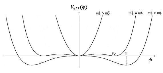
Figure 1: A schematic profile of the effective potential where SSB is a 1st-order phase transition.

Let us now consider the phenomenon of SSB. Here, for constant field configurations, the basic quantity is the effective potential $V_{\rm eff}(\phi)$. Within the class of normalized quantum states $\langle\Psi|\Psi\rangle=1$, this is defined in the infinite volume limit ${{\sf V}}\to\infty$ as

$$V_{\rm eff}(\phi)=\frac{1}{{\sf V}}\cdot{\rm min}_{\Psi}\langle\Psi|H|\Psi\rangle$$ (23)

with the condition

$$\langle\Psi|\Phi|\Psi\rangle=\phi$$ (24)

By expanding around $\phi=0$, the quadratic shape of the effective potential gives the renormalized mass of the symmetric-phase quanta

$$m^{2}_{R}=V^{\prime\prime}_{\rm eff}(\phi)\Big{|}_{\phi=0}$$ (25)

given as a power serious expansion

$$m^{2}_{R}=m^{2}+g^{2}\Delta m^{2}(2)+g^{3}\Delta m^{2}(3)+...$$ (26)

In turn, from the connection between variational principle and the eigenvalue equation for the Hamiltonian, for a translational invariant field configuration, the previous zero-energy condition of the symmetric ground state at $\langle\Psi_{0}|\Phi|\Psi_{0}\rangle=0$ implies

$$V_{\rm eff}(\phi=0)=0$$ (27)

to any finite order in $g$.

The conventional second-order picture of SSB assumes that no non-trivial minima can exist if $m^{2}_{R}\geq 0$. Instead, as indicated by most recent lattice simulations [37, 38, 39] of a pure $\Phi^{4}$ theory, we will adopt the view of SSB as a (weak) first-order phase transition. This means that, with the same Hamiltonian Eq.(14), before reaching the massless $m^{2}_{R}=0$ limit, for some very small $m^{2}_{R}=m^{2}_{c}$ there will arise a first pair of vacua, say with $\langle\Phi\rangle=\pm v_{c}$, which have the same zero energy as the empty vacuum at $\langle\Phi\rangle=0$ see Fig. 1. Therefore the critical mass is defined as that value

$$m^{2}_{c}=V^{\prime\prime}_{\rm eff}(\phi)\Big{|}_{\phi=0}$$ (28)

for which there are $three$ vacuum states with the same energy

$$0=V_{\rm eff}(\phi=0)=V_{\rm eff}(\phi=\pm v_{c})$$ (29)

On the other hand, for $0\leq m^{2}_{R}<m^{2}_{c}$, SSB takes place and the energy of the two degenerate vacua, say $|\Psi_{\pm}\rangle$ with $\langle\Psi_{\pm}|\Phi|\Psi_{\pm}\rangle=\pm v$, will definitely be lower than its value at $\langle\Phi\rangle=0$

$$V_{\rm eff}(\phi=\pm v)<V_{\rm eff}(\phi=0)=0$$ (30)

Explicit calculations, either in the loop expansion [27] or variational [44], indicate that $V_{\rm eff}(\phi=\pm v)$ has a non analytic $\exp(-1/g)$ behaviour. This reflects the basic non perturbative nature of SSB which cannot be found to any finite order in $g$.

Here we emphasize a few aspects:

i) to understand intuitively the first-order nature of the phase transition, the crucial observation is that the quanta of the symmetric phase, besides the +$g\delta^{(3)}(\bf r)$ repulsion, also feel a $-g^{2}\frac{e^{-2mr}}{r^{3}}$ attraction [27] which shows up at the one-loop level and whose range becomes longer and longer in the $m\to 0$ limit. A calculation of the energy density in the dilute-gas approximation, which is equivalent to the one-loop effective potential, indicates that for very small $m$ the attractive tail dominates. Higher-order corrections simply renormalize the strength of these two basic effects [27] whose interplay explains the instability of the symmetric phase producing a $\langle\Phi\rangle\neq 0$

ii) the field fluctuations around each of the two non-symmetric vacua are conveniently described by the shifted field $h(x)\equiv\Phi(x)-\langle\Phi\rangle$, with $\langle h\rangle=0$ by definition. In the realistic case of the Standard Model with a SU(2)xU(1) symmetry, the lowest $h-$field excitation has mass $m_{h}\sim$ 125 GeV as observed at the Large Hadron Collider of CERN. Notice that this $m_{h}$ is conceptually different from the $m_{R}$ discussed above, the two mass parameters describing the quadratic shape of the effective potential at two different values of $\phi$, namely

$$m^{2}_{h}=V^{\prime\prime}_{\rm eff}(\phi)\Big{|}_{\phi=\pm v}$$ (31)

iii) strictly speaking, Wightman’s axioms [40] require a unique vacuum state. The usual way out is that the two states $|\Psi_{\pm}\rangle$, giving the absolute minima of the effective potential, have zero overlap $\langle\Psi_{-}|\Psi_{+}\rangle\to 0$ in the infinite-volume ${{\sf V}}\to\infty$ [45]

iv) due to the equivalence between variational method and eigenvalue equation, the two spontaneously broken vacua $|\Psi_{\pm}\rangle$, at the minima of the effective potential, are the lowest eigenstates of the Hamiltonian. However, by assuming Eq.(18), their energy cannot be zero. Then, from $[P_{i},{L}_{0i}]=iP_{0}$, $P_{i}|\Psi_{\pm}\rangle=0$ and $P_{0}|\Psi_{\pm}\rangle\neq 0$ it follows ${L}_{0i}|\Psi_{\pm}\rangle\neq 0$ so that the two states $|\Psi_{\pm}\rangle$ cannot be Lorentz invariant [46, 47, 48].

Of course, concerning iv), we could define a different free-field limit to preserve the Lorentz invariance of the two $|\Psi_{\pm}\rangle$. To this end, one should first express the field as $\Phi(x)=h(x)+\langle\Phi\rangle$ so that the original $\Phi^{4}$ term will also produce a cubic term $g\langle\Phi\rangle h^{3}$ which reflects the interaction of the $h$-field fluctuation with the vacuum condensate $\langle\Phi\rangle$. Then, $h(x)$ should be quantized in terms of new annihilation and creation operators, say $b({\bf k})$ and $b^{\dagger}({\bf k})$ for $|\Psi_{+}\rangle$ and $c({\bf k})$ and $c^{\dagger}({\bf k})$ for $|\Psi_{-}\rangle$, so that $b({\bf k})|\Psi_{+}\rangle=0$ and $c({\bf k})|\Psi_{-}\rangle=0$. This means that one should select one of the two non-symmetric vacuum states, for instance $|\Psi_{+}\rangle$, and define the normal ordering procedure, in terms of $b({\bf k})$ and $b^{\dagger}({\bf k})$. After having re-defined the free-field limit, the perturbative expansion should also be re-formulated because, now, there is a new dimensionful coupling constant $g\langle\Phi\rangle$ . Finally, the additive constant $\Delta E$ should now be determined by requiring zero energy for $|\Psi_{+}\rangle$ with a change in the Hamiltonian Eq.(14). Correspondingly, the previous symmetric vacuum $|\Psi_{0}\rangle$, would now be higher of the same amount associated with $V_{\rm eff}(\phi=\pm v)$.

With these two different procedures, one has to choose between the Lorentz invariance of the two degenerate minima $|\Psi_{\pm}\rangle$ and the Lorentz invariance of the original $|\Psi_{0}\rangle$. In particular, with the alternative re-arrangement described above, we are implicitly admitting that, even in the simplest case of a one-component, massive $\Phi^{4}$ theory with $g\to 0^{+}$, there is no way to start from the free-field vacuum $|{\rm o}\rangle$ and preserve, in perturbation theory, the basic Lorentz symmetry embodied in the operatorial structure Eqs.(10)-(2) . Perhaps, a way out could be to impose the condition $m^{2}_{R}=m^{2}_{c}$ which fixes the mass of the symmetric phase at the particular critical value where Eq.(29) holds true and the three local minima have all the same zero energy (a choice which, however, would imply the meta-stability of the broken-symmetry phase).

By discarding the particular case $m^{2}_{R}=m^{2}_{c}$, we will then return to our original choice of a Lorentz invariant $|\Psi_{0}\rangle$. The point is that the resulting Lorentz-non-invariance of the two non-symmetric minima $|\Psi_{\pm}\rangle$ has an intuitive physical meaning. Indeed, it reflects the macroscopic occupation of the same quantum state by the basic elementary quanta of $\Phi^{4}$, those described by $a({\bf k})$ and $a^{\dagger}({\bf k})$, and which behave as hard spheres at the asymptotic cutoff scale $\Lambda_{s}$.

To this end, let us consider the field expansion in terms of $a({\bf k})$ and $a^{\dagger}({\bf k})$

$$\Phi({\bf x})=\sum_{\bf k}\frac{1}{\sqrt{2{\sf V}E(k)}}\left[a({\bf k})e^{i{\bf k\cdot x}}+a^{\dagger}({\bf k})e^{-i{\bf k\cdot x}}\right]$$ (32)

and introduce the number of field quanta through the operator

$$\hat{{\sf N}}=\sum_{\bf k}a^{\dagger}_{\bf k}a_{\bf k}$$ (33)

For a temperature $T=0$, following ’t Hooft [26], see also [27], SSB corresponds to a macroscopic number ${\sf N}$ of quanta in the state ${\bf k}=0$ of some reference frame $\Sigma$. In this case, where $\hat{{\sf N}}\sim a^{\dagger}_{0}a_{0}$, one can effectively consider $a_{0}$ as a c-number $\sqrt{{\sf N}}$ with

$$\phi=\langle\Phi\rangle\sim\frac{1}{\sqrt{2{\sf V}m}}~{}2a_{0}\sim\sqrt{\frac{2{\sf N}}{{\sf V}m}}$$ (34)

a density $n\equiv{\sf N}/{\sf V}$ (with ${\sf N}\to\infty$, ${\sf V}\to\infty$ at fixed $n$) given by

$$n\sim{\scriptstyle{\frac{1}{2}}}m\phi^{2}$$ (35)

and mass density $\rho_{m}=(m{\sf N}/{\sf V})$ reproducing the quadratic term ${\scriptstyle{\frac{1}{2}}}m^{2}\phi^{2}$ in the potential.

In this formalism, it will be natural to adopt a particular notation for each of the two degenerate vacua $|\Psi_{\pm}\rangle$, say $|\Psi^{(\Sigma)}_{\pm}\rangle$, which defines the vacuum assignment for that observer which is at rest in $\Sigma$. As we have seen, if these states have a non-zero energy $E_{0}<0$, and thus are not Lorentz invariant, boost operators ${U}^{\prime}$, ${U}^{\prime\prime}$,..will transform non-trivially $|\Psi^{(\Sigma)}_{\pm}\rangle$ into new states $|\Psi^{\prime}_{\pm}\rangle$, $|\Psi^{\prime\prime}_{\pm}\rangle$,… appropriate to moving observers $S^{\prime}$, $S^{\prime\prime}$,..For instance, by defining the boost operator $U^{\prime}=e^{i\lambda^{\prime}{L}_{01}}$ one finds

$$|\Psi^{\prime}_{\pm}\rangle=e^{i\lambda^{\prime}{L}_{01}}|\Psi^{(\Sigma)}_{\pm}\rangle$$ (36)

so that, by using the relations

$$e^{-i\lambda^{\prime}{L}_{01}}~{}{P}_{1}~{}e^{i\lambda^{\prime}{L}_{01}}=\cosh\lambda^{\prime}~{}{P}_{1}+\sinh\lambda^{\prime}~{}{P}_{0}$$ (37)

$$e^{-i\lambda^{\prime}{L}_{01}}~{}{P}_{0}~{}e^{i\lambda^{\prime}{L}_{01}}=\sinh\lambda^{\prime}~{}{P}_{1}+\cosh\lambda^{\prime}~{}{P}_{0}$$ (38)

we obtain

$${{P}_{1}}|\Psi^{\prime}_{\pm}\rangle=E_{0}\sinh\lambda^{\prime}|\Psi^{\prime}_{\pm}\rangle~{}~{}~{}~{}~{}~{}~{}~{}~{}~{}~{}~{}~{}~{}~{}{{P}_{0}}|\Psi^{\prime}_{\pm}\rangle=E_{0}\cosh\lambda^{\prime}|\Psi^{\prime}_{\pm}\rangle$$ (39)

Thus, the physical, realized form of relativity would now contain a preferred frame $\Sigma$ with zero spatial momentum. In a generic moving system $S^{\prime}$, one would instead find

$${{P}_{i}}|\Psi^{\prime}_{\pm}\rangle=E_{0}b_{i}|\Psi^{\prime}_{\pm}\rangle~{}~{}~{}~{}~{}~{}~{}~{}~{}{{P}_{0}}|\Psi^{\prime}_{\pm}\rangle=E_{0}a|\Psi^{\prime}_{\pm}\rangle~{}~{}~{}~{}~{}~{}~{}a^{2}-b_{i}b_{i}=1$$ (42)

We observe that, traditionally, with the exception of Chiao’s [29] mentioned ‘conceptual tensions’, SSB was never believed to be in a potential conflict with Einstein relativity. The motivation being, perhaps, that the mean properties of the condensed phase are summarized into the vacuum expectation value $\langle\Phi\rangle$ of the Higgs field which transforms as a world scalar under the Lorentz group. However, this does not imply that the vacuum state itself is Lorentz invariant. Lorentz transformation operators ${U}^{\prime}$, ${U}^{\prime\prime}$,…could transform non trivially the reference vacuum states $|\Psi^{(\Sigma)}_{\pm}\rangle$ and, yet, for any Lorentz scalar operator ${S}$, i.e. for which $S=(U^{\prime})^{\dagger}SU^{\prime}=(U^{\prime\prime})^{\dagger}SU^{\prime\prime}...$, one would find

$$\langle\Psi^{(\Sigma)}_{\pm}|{S}|\Psi^{(\Sigma)}_{\pm}\rangle=\langle\Psi^{\prime}_{\pm}|{S}|\Psi^{\prime}_{\pm}\rangle=\langle\Psi^{\prime\prime}_{\pm}|{S}|\Psi^{\prime\prime}_{\pm}\rangle...$$ (43)

Another aspect, which is always implicitly assumed but very seldom spelled out, concerns the condition $V_{\rm eff}(\phi=0)=0$. This is usually interpreted as a matter of convention, as if one were actually computing $\Delta V_{\rm eff}(\phi)\equiv V_{\rm eff}(\phi)-V_{\rm eff}(\phi=0)$. However, starting from this apparently innocent assumption, many authors have raised the problem of the non-zero cosmological constant in Einstein’s field equations which is generated by SSB. This problem has only a definite meaning if the condition $V_{\rm eff}(\phi=0)=0$ is not arbitrary but is actually assumed from the start for consistency. With our previous analysis of the symmetric vacuum, we can now understand the motivations of this implicit assumption. Starting from the free-field structure in Eqs.(10)- (2), the condition Eq.(27) expresses the requirement of having a zero-energy vacuum at $\phi=0$ and, therefore, of preserving its Lorentz invariance in the interacting theory. Still, near the critical mass, where Eq.(29) holds true, the induced cosmological constant could be made arbitrarily small .

Truly enough, the previous arguments are rather formal and give no information on the preferred frame $\Sigma$ tight to the reference vacua $|\Psi^{(\Sigma)}_{\pm}\rangle$. For this reason, in the following Sect.3, we will turn our attention to experiments and try to understand if $\Sigma$ really exists and if, eventually, is tight to the CMB as assumed in refs. [19, 20, 21, 22, 23].

3 The basics of the ether-drift experiments

3.1 Which preferred frame?

Looking for the preferred $\Sigma-$frame, the natural candidate is the reference system where the temperature of the CMB looks exactly isotropic or, more precisely, where the CMB Kinematic Dipole [18] vanishes. This dipole is in fact a consequence of the Doppler effect associated with the motion of the Earth ($\beta=V/c)$

$$T(\theta)={{T_{o}\sqrt{1-\beta^{2}}}\over{1-\beta\cos\theta}}$$ (44)

Accurate observations with satellites in space [52] have shown that the measured temperature variations correspond to a motion of the solar system described by an average velocity $V\sim 370$ km/s, a right ascension $\alpha\sim 168^{o}$ and a declination $\gamma\sim-7^{o}$, pointing approximately in the direction of the constellation Leo. This means that, if one sets $T_{o}\sim$ 2.725 K and $\beta\sim 0.00123$, there are angular variations of a few millikelvin

$$\Delta T^{\rm CMB}(\theta)\sim T_{o}\beta\cos\theta\sim\pm 3.36~{}{\rm mK}$$ (45)

which represent by far the largest contribution to the CMB anisotropy.

Therefore, one may ask, could the reference system with vanishing CMB dipole represent a fundamental preferred frame for relativity as in the original Lorentzian formulation? The standard answer is that one should not confuse these two concepts. The CMB is a definite medium and, as such, sets a rest frame where the dipole anisotropy is zero. Our motion with respect to this system has been detected but there is no contradiction with Special Relativity.

Though, to good approximation, this kinematic dipole arises by combining the various forms of peculiar motion which are involved (rotation of the solar system around the center of the Milky Way, motion of the Milky Way toward the center of the Local Group, motion of the Local Group of galaxies in the direction of the Great Attractor…) [52]. Thus, if one could switch-off the local inhomogeneities which produce these peculiar forms of motion, it is natural to imagine a global frame of rest associated with the Universe as a whole. A vanishing CMB dipole could then just indicate the existence of this fundamental system $\Sigma$ that we may conventionally decide to call ‘ether’ but the cosmic radiation itself would not coincide with this form of ether. Due to the group properties of Lorentz transformations, two observers S’ and S”, moving individually with respect to $\Sigma$, would still be connected by a Lorentz transformation with relative velocity parameter fixed by the standard relativistic composition rule . But, as anticipated in the Introduction, ultimate consequences would be far reaching.

The answer cannot be found on pure theoretical grounds and this is why one looks for a small anisotropy of the two-way velocity of light $\frac{\Delta\bar{c}_{\theta}}{c}\neq 0$ in the Earth laboratory. Here, the general consensus is that no genuine ether drift has ever been observed, all measurements (from Michelson-Morley to the most recent experiments with optical resonators) being seen as a long sequence of null results, i.e. typical instrumental effects in experiments with better and better systematics (see e.g. Figure 1 of ref.[56]).

However, this is not necessarily true. In the original measurements, light was propagating in gaseous systems (air or helium at atmospheric pressure) while now, in modern experiments, light propagates in a high vacuum or inside solid dielectrics. Therefore, in principle, the difference with the modern experiments might not depend on the technological progress only but also on the different media that are tested thus preventing a straightforward comparison. This is even more true if one takes into account that, in the past, greatest experts (as Hicks and Miller) have seriously questioned the traditional null interpretation of the very early measurements. The observed ‘fringe shifts’, although much smaller than the predictions of classical physics, were often non negligible as compared to the extraordinary sensitivity of the interferometers. It is then conceivable that, in some alternative framework, the small residuals could acquire a physical meaning. As a definite example, in the following Subsect. 3.2, we will summarize the theoretical scheme of refs.[31, 32, 33, 34] starting with the old experiments. The modern experiments will be considered in Subsect.3.3.

3.2 The old experiments in gaseous media

In the old experiments in gases (Michelson-Morley, Miller, Tomaschek, Kennedy, Illingworth, Piccard-Stahel, Michelson-Pease-Pearson, Joos) [57]-[66], with refractive index ${\cal N}=1+\epsilon$, the velocity of light in the interferometers, say $c_{\gamma}$, was not the same parameter $c$ of Lorentz transformations. Hence, assuming their exact validity, deviations from isotropy could only be due to the small fraction of refracted light which keeps track of the velocity of matter with respect to $\Sigma$ and produces a direction-dependent refractive index. As anticipated in the Introduction, from symmetry arguments valid in the $\epsilon\to 0$ limit [31, 32, 33, 34], one would then expect a two-way velocity

$$\bar{c}_{\gamma}(\theta) = {{2c_{\gamma}(\theta)c_{\gamma}(\pi+\theta)}\over{c_{\gamma}(\theta)+c_{\gamma}(\pi+\theta)}}\sim{{c}\over{{\cal N}}}~{}\left[1-\epsilon\beta^{2}\left(1+\cos^{2}\theta\right)\right]\equiv{{c}\over{\bar{\cal N}(\theta)}}$$ (46)

with an effective $\theta-$dependent refractive index

$$\bar{\cal N}(\theta)\sim{\cal N}~{}[1+\epsilon\beta^{2}(1+\cos^{2}\theta)]$$ (47)

and a fractional anisotropy

$${{\Delta\bar{c}_{\theta}}\over{c}}={{\bar{c}_{\gamma}(\pi/2+\theta)-\bar{c}_{\gamma}(\theta)}\over{c}}\sim\epsilon~{}\beta^{2}\cos 2\theta$$ (48)

In the above relations, $\beta\equiv v/c$, with $v$ and $\theta=0$ indicating respectively the magnitude and the direction of the drift in the plane of the interferometer.

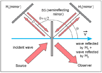
Figure 2: A schematic illustration of the Michelson interferometer. Note that, by computing the transit times and the resulting fringe shifts Eq.(49), we are assuming the validity of Lorentz transformations so that the length of a rod does not depend on its orientation, in the frame $S^{\prime}$ where it is at rest.

By introducing the optical path $D$, see Fig.2, and the light wavelength $\lambda$, this would produce a fringe pattern

$${{\Delta\lambda(\theta)}\over{\lambda}}={{2D}\over{\lambda}}~{}{{\Delta\bar{c}_{\theta}}\over{c}}\sim{{2D}\over{\lambda}}~{}\epsilon~{}{{v^{2}}\over{c^{2}}}\cos 2\theta$$ (49)

so that the dragging of light in the Earth frame is described as a pure 2nd-harmonic effect which is periodic in the range $[0,\pi]$, as in the classical theory (see e.g. [67]), with the exception of its amplitude

$$A_{2}={{2D}\over{\lambda}}~{}\epsilon~{}{{{v}^{2}}\over{c^{2}}}$$ (50)

This is suppressed by the factor $2\epsilon$ relatively to the classical amplitude for the orbital velocity of 30 km/s

$$A^{\rm class}_{2}={{D}\over{\lambda}}(\frac{30~{}{\rm km/s}}{c})^{2}$$ (51)

This difference could then be re-absorbed into an observable velocity which depends on the gas refractive index

$$v^{2}_{\rm obs}\sim 2\epsilon v^{2}$$ (52)

and is the very small velocity $5-10$ km/s traditionally extracted from the classical analysis of the early experiments through the relation

$$v_{\rm obs}\sim 30~{}{\rm km/s}~{}\sqrt{\frac{A^{\rm EXP}_{2}}{A^{\rm class}_{2}}}$$ (53)

see e.g. Fig.3.

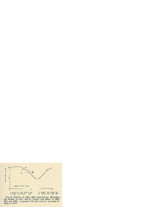
Figure 3: The observable velocity Eq.(53) reported by Miller [58] for various experiments.

Thus, no surprise that the resulting ${{|\Delta\bar{c}_{\theta}|}\over{c}}\sim\epsilon(v^{2}/c^{2})$ was much smaller than the classical expectation. For instance, in the old experiments in air (at room temperature and atmospheric pressure where $\epsilon\sim 2.8\cdot 10^{-4}$) a typical value was ${{|\Delta\bar{c}_{\theta}|_{\rm exp}}\over{c}}\sim 3\cdot 10^{-10}$. By assuming the classical relations (51),(53), this was originally interpreted as an observable velocity $v_{obs}\sim 7.3$ km/s but, by using Eq.(52), this observable velocity would now correspond to a true kinematic velocity $v\sim 310$ km/s. Analogously, in the old experiment in gaseous helium (at room temperature and atmospheric pressure, where $\epsilon\sim 3.3\cdot 10^{-5}$), a typical value was ${{|\Delta\bar{c}_{\theta}|_{\rm exp}}\over{c}}\sim 2.2\cdot 10^{-11}$. This was classically interpreted as an (observable) velocity of 2 km/s but would now correspond to a true kinematical value $v\sim 240$ km/s.

Another observation concerns the time-dependence of the data and the precise definition of $v$ and $\theta=0$ in the above relations. Traditionally, for short-time observations of a few days, where there can be no sizeable change in the orbital motion of the Earth, the genuine signal for a preferred frame was consisting in the regular modulations induced by the Earth rotation. Instead the data had an irregular behavior indicating sizeably different directions of the drift at the same hour on consecutive days. This was a strong argument to interpret the small residuals as typical instrumental artifacts. However, this conclusion derives from the traditional identification of the local velocity field which describes the drift, say $v_{\mu}(t)$, with the corresponding projection of the global Earth motion, say $\tilde{v}_{\mu}(t)$. This identification is equivalent to a form of regular, laminar flow where global and local velocity fields coincide and, in principle, may be incorrect.

The model of ether drift adopted in refs. [31, 32, 33, 34] starts from Maxwell’s original argument [68]. After having considered all known properties of light, he was driven to consider the idea of a substratum: ”…We are therefore obliged to suppose that the medium through which light is propagated is something distinct from the transparent media known to us…”. He was calling this substratum ”ether” while, today, we prefer to call it ”physical vacuum”. However, this is irrelevant. The essential point for the propagation of light, e.g. inside an optical cavity, is that, differently from the solid parts of the apparatus, this physical vacuum is not totally entrained with the Earth motion. Therefore, to explain the irregular character of the data, the original idea of refs.[69, 70] was to model this vacuum as a turbulent fluid or, more precisely, as a fluid in the limit of zero viscosity . Then, the simple picture of a laminar flow is no more obvious due to the subtlety of the infinite-Reynolds-number limit, see e.g. Sect. 41.5 in Vol.II of Feynman’s lectures [80]. Namely, beside $v_{\mu}(t)=\tilde{v}_{\mu}(t)$, there is also another solution where $v_{\mu}(t)$ is a continuous, nowhere differentiable velocity field [81, 82]. This leads to the idea of a signal with a fundamental stochastic nature as when turbulence, at small scales, becomes homogeneous and isotropic. One should thus first analyze the data for ${{\Delta\bar{c}_{\theta}(t)}\over{c}}$ and extract the (2nd-harmonic) phase and amplitude $A_{2}(t)$ by concentrating on the latter which is positive definite and remains non-zero under any averaging procedure.

For a quantitative description, let us assume a set of kinematic parameters $(V,\alpha,\gamma)$ for the Earth cosmic motion, a latitude $\phi$ of the laboratory and a given sidereal time $\tau=\omega_{\rm sid}t$ (with $\omega_{\rm sid}\sim{{2\pi}\over{23^{h}56^{\prime}}}$). Then $\tilde{v}(t)=V|\sin z(t)|$ is the magnitude of the projection in the plane of the interferometer, $\sin z(t)$ being defined by [83]

$$\cos z(t)=\sin\gamma\sin\phi+\cos\gamma\cos\phi\cos(\tau-\alpha)$$ (54)

In this scheme, the amplitude $\tilde{A}_{2}(t)$ associated with the global motion is

$$\tilde{A}_{2}(t)\sim{{2D}\over{\lambda}}\cdot\epsilon\cdot{{V^{2}\sin^{2}z(t)}\over{c^{2}}}$$ (55)

Although the local, irregular $v_{\mu}(t)$ is not a differentiable function it could still be simulated in terms of random Fourier series [81, 84, 85]. This method was adopted in refs.[31, 32, 33, 34] in a simplest uniform-probability model, where the kinematic parameters of the global $\tilde{v}_{\mu}(t)$ are just used to fix the boundaries for the local random $v_{\mu}(t)$. The essential ingredients are summarized in the Appendix.

We emphasize that the instantaneous, irregular $A_{2}(t)$ is very different from the smooth $\tilde{A}_{2}(t)$. However, the relation with the statistical average $\langle A_{2}(t)\rangle_{\rm stat}$ is very simple

$$\langle A_{2}(t)\rangle_{\rm stat}\sim{{\pi^{2}}\over{18}}\cdot\tilde{A}_{2}(t)\sim{{2D}\over{\lambda}}\cdot{{\pi^{2}}\over{18}}~{}\epsilon~{}\frac{V^{2}\sin^{2}z(t)}{c^{2}}$$ (56)

Furthermore, by using Eq.(54), if the amplitude is measured at various sidereal times, one can also get information on the angular parameters $\alpha$ and $\gamma$.

Altogether, those old measurements ${{|\Delta\bar{c}_{\theta}|_{\rm exp}}\over{c}}\sim 3\cdot 10^{-10}$ and ${{|\Delta\bar{c}_{\theta}|_{\rm exp}}\over{c}}\sim 2.2\cdot 10^{-11}$, respectively for air or gaseous helium at atmospheric pressure, can thus be interpreted in three different ways: a) as 7.3 and 2 km/s, in a classical picture b) as 310 and 240 km/s, in a modern scheme and in a smooth picture of the drift c) as 418 and 324 km/s, in a modern scheme but now allowing for irregular fluctuations of the signal. In this last case, in fact, by replacing Eq.(55) with Eq.(56), from the same data one would now obtain kinematical velocities which are larger by a factor $\sqrt{18/{\pi^{2}}}\sim 1.35$. In this third interpretation, the average of the two values agrees very well with the CMB velocity of 370 km/s. The comparison with all classical experiments is shown in Table 1.

Table 1: The average 2nd-harmonic amplitudes of classical ether-drift experiments. These were extracted from the original papers by averaging the amplitudes of the individual observations and assuming the direction of the local drift to be completely random (i.e. no vector averaging of different sessions). These experimental values are then compared with the full statistical average Eq.(56) for a projection 250 km/s $\lesssim V|\sin z(t)|\lesssim$ 370 km/s of the Earth motion in the CMB and refractivities $\epsilon=2.8\cdot 10^{-4}$ for air and $\epsilon=3.3\cdot 10^{-5}$ for gaseous helium. The experimental value for the Morley-Miller experiment is taken from the observed velocities reported in Miller’s Figure 4, here our Fig.3. The experimental value for the Michelson-Pease-Pearson experiment refers to the only known session for which the fringe shifts are reported explicitly [65] and where the optical path was still fifty-five feet. The symbol $\pm....$ means that the experimental uncertainty cannot be determined from the available informations. The table is taken from ref.[34].

Experiment	gas	$A^{\rm EXP}_{2}$	${{2D}\over{\lambda}}$	$\langle A_{2}(t)\rangle_{\rm stat}$
Michelson(1881)	air	$(7.8\pm....)\cdot 10^{-3}$	$4\cdot 10^{6}$	$(0.7\pm 0.2)\cdot 10^{-3}$
Michelson-Morley(1887)	air	$(1.6\pm 0.6)\cdot 10^{-2}$	$4\cdot 10^{7}$	$(0.7\pm 0.2)\cdot 10^{-2}$
Morley-Miller(1902-1905)	air	$(4.0\pm 2.0)\cdot 10^{-2}$	$1.12\cdot 10^{8}$	$(2.0\pm 0.7)\cdot 10^{-2}$
Miller(1921-1926)	air	$(4.4\pm 2.2)\cdot 10^{-2}$	$1.12\cdot 10^{8}$	$(2.0\pm 0.7)\cdot 10^{-2}$
Tomaschek (1924)	air	$(1.0\pm 0.6)\cdot 10^{-2}$	$3\cdot 10^{7}$	$(0.5\pm 0.2)\cdot 10^{-2}$
Kennedy(1926)	helium	$<0.002$	$7\cdot 10^{6}$	$(1.4\pm 0.5)\cdot 10^{-4}$
Illingworth(1927)	helium	$(2.2\pm 1.7)\cdot 10^{-4}$	$7\cdot 10^{6}$	$(1.4\pm 0.5)\cdot 10^{-4}$
Piccard-Stahel(1928)	air	$(2.8\pm 1.5)\cdot 10^{-3}$	$1.28\cdot 10^{7}$	$(2.2\pm 0.8)\cdot 10^{-3}$
Mich.-Pease-Pearson(1929)	air	$(0.6\pm...)\cdot 10^{-2}$	$5.8\cdot 10^{7}$	$(1.0\pm 0.4)\cdot 10^{-2}$
Joos(1930)	helium	$(1.4\pm 0.8)\cdot 10^{-3}$	$7.5\cdot 10^{7}$	$(1.5\pm 0.6)\cdot 10^{-3}$

Notice the substantial difference with the analogous summary Table I of ref.[86] where those authors were comparing with the much larger classical amplitudes Eq.(51) and emphasizing the much smaller magnitude of the experimental fringes. Here, is just the opposite. In fact, our theoretical statistical averages are often smaller than the experimental results indicating, most likely, the presence of systematic effects in the measurements.

At the same time, by adopting Eq.(56), from the experiments in air we find $\tilde{v}_{\rm air}\sim 418\pm 62$ km/s and from the two experiments in gaseous helium $\tilde{v}_{\rm helium}\sim 323\pm 70$ km/s, with a global average $\langle\tilde{v}\rangle\sim 376\pm 46$ km/s which agrees well with the 370 km/s from the CMB observations. Even more, from the two most precise experiments of Piccard-Stahel (the measurements performed on ground in Bruxelles and at Mt. Rigi in Switzerland) and those made in Jena by Georg Joos we find, in our stochastic scheme, two determinations, $\tilde{v}=360^{+85}_{-110}$ km/s and $\tilde{v}=305^{+85}_{-100}$ km/s respectively, whose average $\langle\tilde{v}\rangle\sim 332^{+60}_{-80}$ km/s reproduces to high accuracy the projection of the CMB velocity at a typical Central-Europe latitude. Finally, by using Eq.(54) and fitting the amplitudes obtained from Joos’ observations (data collected at steps of 1 hour to cover the sidereal day) one finds [31, 33] $\alpha({\rm fit-Joos})=(168\pm 30)$ degrees and $\gamma({\rm fit-Joos})=(-13\pm 14)$ degrees which are consistent with the present values $\alpha({\rm CMB})\sim$ 168 degrees and $\gamma({\rm CMB})\sim-$7 degrees.

As it often happens, symmetry arguments can successfully describe a phenomenon regardless of the physical mechanisms behind it. The same is true here with our relation ${{|\Delta\bar{c}_{\theta}|}\over{c}}\sim\epsilon(v^{2}/c^{2})$. It gives a consistent description of the data but does not explain the ultimate origin of the tiny observed anisotropy in the gaseous systems. For instance, as a first mechanism, we considered the possibility of different polarizations in different directions in the dielectric, depending on its state of motion. However, if this works in weakly bound gaseous matter, the same mechanism should also work in a strongly bound solid dielectric, where the refractivity is $({\cal N}_{\rm solid}-1)=O(1)$, and thus produce a much larger ${{|\Delta\bar{c}_{\theta}|}\over{c}}\sim({\cal N}_{\rm solid}-1)(v^{2}/c^{2})\sim 10^{-6}$. This is in contrast with the Shamir-Fox [89] experiment in perspex where the observed value was smaller by orders of magnitude. We have thus re-considered [35, 32, 33] the traditional thermal interpretation [90, 86] of the observed residuals. The idea was that, in a weakly bound system as a gas, a small temperature difference $\Delta T^{\rm gas}(\theta)$, of a millikelvin or so, in the air of the two optical arms could produce a difference in the refractive index and a light anisotropy proportional to $\epsilon_{\rm gas}\Delta T^{\rm gas}(\theta)/T$, where $T\sim$ 300 K is the temperature of the laboratory. Miller was aware of this potentially large effect [58, 91] and objected that casual changes of the ambiance temperature would largely cancel when averaging over many measurements. Only temperature effects with a definite angular periodicity would survive. The overall consistency, in our scheme, of different experiments would now indicate that such $\Delta T^{\rm gas}(\theta)$ must have a non-local origin. As anticipated, this could be due to the non-zero momentum flow Eq.(42). Or it could reflect the interactions with the background radiation which transfer a part of $\Delta T^{\rm CMB}(\theta)$ in Eq.(45) and thus bring the gas out of equilibrium. Those old estimates were, however, slightly too large. In fact, in the ideal-gas approximation, from the Lorentz-Lorenz equation for the molecular polarizability, one actually finds [32, 33, 34] $\Delta T^{\rm gas}(\theta)=(0.2-0.3)$ mK . For the CMB case, this would mean that the interactions of the gas with the CMB photons are so weak that, on average, the induced temperature differences in the optical paths were only 1/10 of the $\Delta T^{\rm CMB}(\theta)$ in Eq.(45). Nevertheless, whatever its precise origin, this typical magnitude can help intuition. In fact, it can explain the quantitative reduction of the effect in the vacuum limit where $\epsilon_{\rm gas}\to 0$ and the qualitative difference with solid dielectrics where such small temperature differences cannot produce any appreciable deviation from isotropy in the rest frame of the medium.

Now, admittedly, the idea that small modifications of the gaseous matter, produced by the tiny CMB temperature variations, can be detected by precise optical measurements in a laboratory, while certainly unconventional, has not the same implications of a genuine preferred-frame effect due to the vacuum structure. Still, this thermal explanation of the small residuals in gases has an important predictive power. In fact, it implies that if a tiny, but non-zero, fundamental signal were definitely detected in vacuum then, with very precise measurements, the same universal signal should also show up in a solid dielectric where temperature differences of a fraction of millikelvin become irrelevant. Detecting such ‘non-thermal’ light anisotropy, for the same cosmic motion indicated by the CMB observations, would finally confirm the idea of $\Sigma-$frame assumed in refs. [19, 20, 21, 22, 23].

3.3 The modern experiments in vacuum and solid dielectrics

This expectation of a ‘non-thermal’ light anisotropy, which could be detected in vacuum and in solid dielectrics, was then compared with the modern experiments where ${{\Delta\bar{c}_{\theta}}\over{c}}\sim{{\Delta\nu(\theta)}\over{\nu_{0}}}$ is now extracted from the frequency shift of two optical resonators see Fig.4.

By starting with vacuum resonators, after averaging many observations, the present limit is a residual $\langle{{\Delta\bar{c}_{\theta}}\over{c}}\rangle=10^{-18}-10^{-19}$. However, this just reflects the very irregular nature of the signal because its typical instantaneous magnitude ${{|\Delta\bar{c}_{\theta}(t)|_{v}}\over{c}}\sim 10^{-15}$ is about 1000 times larger, see Fig.5. This $10^{-15}$ signal is found with vacuum resonators [95]$-$[100] made of different materials, operating at room temperature and/or in the cryogenic regime. As such, it cannot be interpreted as a spurious effect, e.g. thermal noise [101].

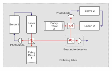
Figure 4: The scheme of a modern ether-drift experiment. The light frequencies are first stabilized by coupling the lasers to Fabry-Perot optical resonators. The frequencies $\nu_{1}$ and $\nu_{2}$ of the resonators are then compared in the beat note detector which provides the frequency shift $\Delta\nu(\theta)=\nu_{1}(\pi/2+\theta)-\nu_{2}(\theta)$. For a review, see e.g. [102].

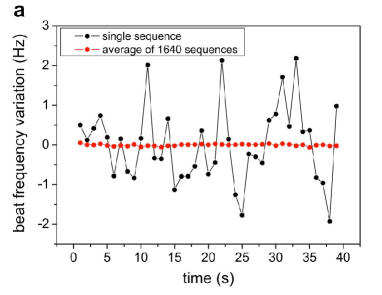
Figure 5: The experimental frequency shift reported in Fig.9(a) of ref.[96] (courtesy Optics Communications). The black dots give the instantaneous signal, the red dots give the signal averaged over 1640 sequences. For a laser frequency $\nu_{0}=2.8\cdot 10^{14}$ Hz a $\Delta\nu=\pm 1$ Hz corresponds to a fractional value $\Delta\nu/\nu_{0}$ of about $\pm 3.5\cdot 10^{-15}$.

In the same model discussed for the classical experiments, we are thus lead to the concept of a refractive index ${\cal N}_{v}$ for the vacuum or, more precisely, for the physical vacuum which is established in an apparatus placed on the Earth surface. This ${\cal N}_{v}$ should differ from unity at the $10^{-9}$ level, in order to give ${{|\Delta\bar{c}_{\theta}(t)|_{v}}\over{c}}\sim({\cal N}_{v}-1)~{}(v^{2}(t)/c^{2})~{}\sim 10^{-15}$, and thus would fit with ref.[103] where, for an apparatus placed on the Earth surface, a vacuum refractivity $\epsilon_{v}\sim(2G_{N}M/c^{2}R)\sim 1.4\cdot 10^{-9}$ was considered, $G_{N}$ being the Newton constant and $M$ and $R$ the mass and radius of the Earth. The idea is that, if the curvature observed in a gravitational field reflects local deformations of the physical space-time units and of the velocity of light [104], for an apparatus on the Earth surface, there could be a tiny difference with that ideal free-fall environment which, in the presence of gravitational effects, is always assumed to define operationally the limit where the velocity of light in vacuum $c_{\gamma}$ coincides with the parameter $c$ of Lorentz transformations. This would reflect the physical difference which, indeed, exists [103] between an observer in a true free-falling elevator and the modified situation of an observer which is in free fall in the same external potential but is now carrying on board a heavy mass $M$, see Fig.6.

Therefore, if $\delta U$ is the extra Newtonian potential produced by the heavy mass $M$ at the experimental setup, the vacuum refractivity, for system (b), can be expressed as

$$\epsilon_{v}={\cal N}_{v}-1\sim{{\chi}\over{2}}~{}\left({{2|\delta U|}\over{c^{2}}}\right)$$ (57)

In General Relativity one assumes $\chi=0$ while the two non-zero values, $\chi=$ 1 or 2, account for the two alternatives traditionally reported in the literature for the effective refractive index in a gravitational potential. For $\chi=2$, the resulting refractivity is the same reported by Eddington [105] to explain in flat space the observed deflection of light in a gravitational field. A difference is found with Landau’s and Lifshitz’ textbook [106] where the vacuum refractive index entering the constitutive relations is instead defined as ${\cal N}_{v}\sim 1+{{|\delta U|}\over{c^{2}}}$. We address to Broekaert’s article [104], and in particular to his footnote ³, for a more detailed discussion of the two choices of $\chi$.

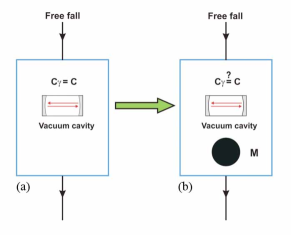
Figure 6: A heavy mass $M$ is carried on board of a freely-falling system, case (b). With respect to the ideal case (a), the mass $M$ modifies the local space-time units and could introduce a vacuum refractive index ${\cal N}_{v}\neq 1$ so that now $c_{\gamma}\neq c$. With a preferred frame, one would then expect off-diagonal elements $g_{0i}\sim 2({\cal N}_{v}-1)(v_{i}/c)$ in the effective metric which describes light propagation for the (b) reference system.

In our case, of an observer on the Earth surface, by introducing the Newton constant, the radius $R$ and the mass $M$ of the Earth, so that $\delta U={{G_{N}M}\over{R}}$, we can express the refractivity as

$$\epsilon_{v}\sim{{\chi}\over{2}}~{}1.4\cdot 10^{-9}$$ (58)

Addressing to ref.[34], here we just report the comparison with ref.[100] which, at present, is the most precise experiment in vacuum. We compared with the average instantaneous variation of the frequency shift over 1 second, see their Fig.3, bottom part. This is defined by the Root Square of the Allan Variance (RAV) (for $\tau_{0}\sim$ 1 second)

$$\left[\sigma_{A}(\Delta\nu,\tau_{0})\right]_{\rm exp}\sim 0.24~{}{\rm Hz}$$ (59)

or, in units of the reference frequency $\nu_{0}=2.8\cdot 10^{14}$ Hz (for $\tau_{0}\sim$ 1 second)

$$\left[\sigma_{A}(\frac{\Delta\nu}{\nu_{0}},\tau_{0})\right]_{\rm exp}~{}\sim 8.5\cdot 10^{-16}~{}~{}~{}~{}~{}~{}~{}~{}~{}~{}~{}~{}~{}~{}~{}~{}~{}~{}{\rm ref.\cite[cite]{[\@@bibref{}{schiller2015}{}{}]}}$$ (60)

As discussed in ref.[34], our instantaneous, stochastic signal is, to very good approximation, a pure white noise for which the RAV coincides with the standard variance. At the same time, for a very irregular signal where $\langle\Delta\nu\rangle=0$ the standard variance $\sigma(\Delta\nu)$ coincides with the average magnitude $\langle|\Delta\nu|\rangle$. Therefore, since in our stochastic model, the average magnitude of the dimensionless frequency shift ${{\Delta\nu(\theta)}\over{\nu_{0}}}\sim{{\Delta\bar{c}_{\theta}}\over{c}}$ is given in Eq.(56), we find (for $\tau_{0}\sim$ 1 second)

$$\left[\sigma_{A}(\frac{\Delta\nu}{\nu_{0}},\tau_{0})\right]_{\rm theor}\sim\left[\frac{\langle|\Delta\nu|\rangle}{\nu_{0}}\right]_{\rm theor}~{}\sim{{\pi^{2}}\over{18}}\cdot\epsilon_{v}\cdot{{V^{2}}\over{c^{2}}}\sin^{2}z(t)$$ (61)

In this way, by replacing Eq.(58), and for a projection 250 km/s $\lesssim V\sin z(t)\lesssim$ 370 Km/s, for $\tau_{0}\sim$ 1 second, our prediction for the RAV can finally be expressed as

$$\left[\sigma_{A}(\frac{\Delta\nu}{\nu_{0}},\tau_{0})\right]_{\rm theor}~{}\sim{{\chi}\over{2}}\cdot(8.5\pm 3.5)\cdot 10^{-16}$$ (62)

By comparing with Eq.(60), we see that the data definitely favor $\chi=2$, which is the only free parameter of our scheme. Also, the very good agreement with our simulated value indicates that, at least for an integration time of 1 second, the corrections to our model should be negligible .

Let us now compare with the modern experiments in solid dielectrics, in particular with the very precise ref.[56]. This is a cryogenic experiment, with microwaves of 12.97 GHz, where almost all electromagnetic energy propagates in a medium, sapphire, with refractive index of about 3 (at microwave frequencies). As anticipated, with a thermal interpretation of the residuals in gaseous media, we expect that a fundamental $10^{-15}$ vacuum anisotropy could also become visible here.

Following refs.[32, 33, 34], we first observe that for ${\cal N}_{v}=1+\epsilon_{v}$ there will be a very tiny difference between the refractive index defined relatively to the ideal vacuum value $c$ and the refractive index relatively to the physical isotropic vacuum value $c/{\cal N}_{v}$ measured on the Earth surface. The relative difference between these two definitions is proportional to $\epsilon_{v}\lesssim 10^{-9}$ and, for all practical purposes, can be ignored. All materials would now exhibit, however, the same background vacuum anisotropy. To this end, let us replace the average isotropic value

$${{c}\over{{\cal N}_{\rm solid}}}\to{{c}\over{{\cal N}_{v}{\cal N}_{\rm solid}}}$$ (63)

and then use Eq.(47) to replace ${\cal N}_{v}$ in the denominator with its $\theta-$dependent value

$$\bar{\cal N}_{v}(\theta)\sim 1+\epsilon_{v}\beta^{2}(1+\cos^{2}\theta)$$ (64)

This is equivalent to define a $\theta-$dependent refractive index for the solid dielectric

$${{\bar{\cal N}_{\rm solid}(\theta)}\over{{\cal N}_{\rm solid}}}\sim 1+\epsilon_{v}\beta^{2}(1+\cos^{2}\theta)$$ (65)

so that

$$\left[{\bar{c}_{\gamma}(\theta)}\right]_{\rm solid}={{c}\over{\bar{\cal N}_{\rm solid}(\theta)}}\sim{{c}\over{{\cal N}_{\rm solid}}}\left[1-\epsilon_{v}\beta^{2}(1+\cos^{2}\theta)\right]$$ (66)

with an anisotropy

$${{\left[\Delta\bar{c}_{\theta}\right]_{\rm solid}}\over{\left[c/{\cal N}_{\rm solid}\right]}}\sim\epsilon_{v}\beta^{2}\cos 2\theta$$ (67)

In this way, a genuine vacuum effect, if there, could also be detected in a solid dielectric.

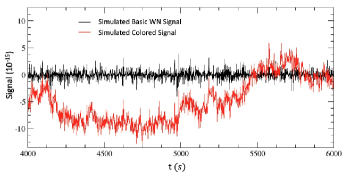
Figure 7: We report two typical sets of 2000 seconds for our basic white-noise (WN) signal and its colored version obtained by Fourier transforming the spectral amplitude of ref.[56]. The boundaries of the random velocity components Eqs.(85) and (86) were defined by Eq.(89) by plugging in Eq.(79) the CMB kinematical parameters, for a sidereal time $t=4000-6000$ seconds and for the latitude of Berlin-Duesseldorf, see the Appendix. The figure is taken from ref.[34].

In ref.[34], a detailed comparison with [56] was presented. First, from Figure 3(c) of [56], it was seen that the spectral amplitude of this particular apparatus becomes flat at frequencies $\omega\geq 0.5$ Hz indicating that the white-noise branch of the signal reaches its minimum value for an integration time $\tau_{0}\sim$ 1 second (at which the other spurious disturbances are still negligible). These data for the spectral amplitude were then fitted to an analytic, power-law form to describe the lower-frequency part 0.001 Hz $\leq\omega\leq 0.5$ Hz which reflects apparatus-dependent disturbances. This fitted spectrum was then used to generate a signal by Fourier transform. Finally, very long sequences of this signal were stored to produce “colored” version of our basic white-noise signal.

To get a qualitative impression of the effect, we report in Fig.7 a sequence of our basic white-noise signal and a sequence of its colored version. By averaging over many 2000-second sequences of this type, the corresponding RAV’s for the two signals are then reported in Fig.8. The experimental RAV extracted from Figure 3(b) of ref.[56] is also reported (for the non-rotating setup). At this stage, the agreement of our simulated, colored signal with the experimental data remains satisfactory only up $\tau=$ 50 seconds. Reproducing the signal at larger $\tau$’s will require further efforts but this is not relevant here, our scope being just to understand the modifications of our stochastic signal near the 1-second scale.

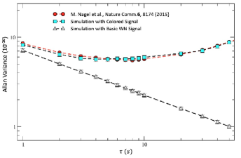
Figure 8: We report the Allan variance for the fractional frequency shift obtained from many simulations of sequences of 2000 seconds for our basic white-noise (WN) signal and for its colored version, see Fig.7. The direct experimental results of ref.[56], for the non-rotating setup, are also shown. The figure is taken from ref.[34].

As one can check from Fig.3(b) of ref.[56], the value of the experimental RAV for the fractional frequency shift (at $\tau_{0}=1$ second) is

$$\sigma_{A}({{\Delta\nu}\over{\nu_{0}}},\tau_{0})_{\rm exp}\sim 8.5\cdot 10^{-16}~{}~{}~{}~{}~{}~{}~{}~{}~{}~{}~{}~{}~{}~{}~{}~{}~{}~{}{\rm ref.\cite[cite]{[\@@bibref{}{nagelnature}{}{}]}}$$ (68)

This is precisely the same value Eq.(60) that we extracted from ref.[100] after normalizing their experimental result $\sigma_{A}(\Delta\nu,\tau_{0})_{\rm exp}\sim$ 0.24 Hz to their laser frequency $\nu_{0}=2.8\cdot 10^{14}$ Hz. At the same time, it also agrees with our Eq.(62) $\sigma_{A}({{\Delta\nu}\over{\nu_{0}}},\tau_{0})_{\rm theor}=(8.5\pm 3.5)\cdot 10^{-16}$ for $\chi=2$. Therefore this beautiful agreement, between ref.[100] (a vacuum experiment at room temperature) and ref.[56] (a cryogenic experiment in a solid dielectric), on the one hand, and with our Eq.(62), on the other hand, confirms our interpretation of the experiments in terms of a stochastic signal associated with the Earth cosmic motion within the CMB.

Two ultimate experimental checks still remain. First, one should try to detect our predicted, daily variations Eq.(62) in the range $(5-12)\cdot 10^{-16}$ corresponding to 250 km/s $\lesssim V\sin z(t)\lesssim$ 370 Km/s. Due to the excellent systematics, these should remain visible with both experimental setups. Second, one more complementary test should be performed by placing the vacuum (or solid dielectric) optical cavities on board of a satellite, as in the OPTIS proposal [107]. In this ideal free-fall environment, as in panel (a) of our Fig.6, the typical instantaneous frequency shift should be much smaller (by orders of magnitude) than the corresponding $10^{-15}$ value measured with the same interferometers on the Earth surface.

4 Summary and outlook

In this paper, we have considered one of the most controversial aspects of Quantum Mechanics, namely the apparent violation of Einstein locality and the conflict with (Einstein) relativity. Since the original paper by Einstein-Podolski-Rosen (EPR) [3] and through the work of Bell [4], many authors have thus arrived to the conclusion that, to dispose of the causality paradox in a realistic interpretation of the theory, it may be natural to introduce a special frame of reference $\Sigma$ for relativity. Then, one can consider the idea that some ‘Quantum Information’ propagates at a vastly superluminal speed $v_{QI}\gg c$, with standard Quantum Mechanics corresponding to the $v_{QI}\to\infty$ limit. In this way, by comparing with experiments [19, 20, 21, 22, 23] one finds the lower bounds $v_{QI}>10^{4}-10^{6}c$ if the preferred $\Sigma-$frame is identified with the reference system where the Cosmic Microwave Background (CMB) is seen isotropic, namely that particular system where the observed CMB Kinematic Dipole [18] vanishes exactly.

A frequent objection to this idea of a preferred frame is that, after all, Quantum Mechanics is not a fundamental description of the world. One should instead start from a fundamental QFT which incorporates the locality requirement. For this reason we have tried to understand if, in the perspective of an underlying, fundamental QFT, there could be a missing logical step which prevents to deduce that Einstein Special Relativity, with no preferred frame, is the physically realized version of relativity. Einstein Relativity is always assumed when computing S-matrix elements for elementary particle processes but what one is actually using is the machinery of Lorentz transformations whose first, complete derivation dates back to Larmor and Lorentz who were assuming the existence of a fundamental state of rest (the ether).

In particular, in our opinion, an element missed so far derives from the present view of the lowest energy state in elementary particle theory which is called ”vacuum” but should actually be thought as a condensate of elementary quanta. So far, one has always been imposing the traditional constraint that, as far as local operators are concerned, the only possible vacuum expectation values are those which transform as world scalars under the Lorentz group.

But, as discussed in Sect.2, this does not imply the vacuum to be a Lorentz-invariant state. This would rather require the vacuum to be annihilated by the generators of the Lorentz boosts. In four space-time dimensions, this requirement is only fulfilled for the free-field case which, by definition, has a unique vacuum and where the simplest prescription of the Wick, normal ordering allows for a consistent representation of the Poincaré algebra. Instead, in the interacting theory and in the presence of Spontaneous Symmetry Breaking, one can meaningfully argue that the physically realized form of relativity contains a preferred reference system $\Sigma$.

However, since our arguments have not the status of a theorem, to decide if $\Sigma$ really exists we have then looked for definite experimental indications from the ether-drift experiments by summarizing in Sect.3 the extensive work of refs.[31]-[35], where all data from Michelson-Morley to the present experiments with optical resonators were considered. Ours is not the only possible scheme to analyze the data but, still, in this theoretical framework, which assumes the validity of Lorentz transformations and allows for irregular fluctuations of the signal, the long sought $\Sigma-$frame tight to the CMB is naturally emerging.

Finally, before closing our paper, we will return to our starting point: the idea that eventually the non-locality of Quantum Mechanics could be understood as the consequence of some ‘Quantum Information’ which propagates at a vastly superluminal speed $v_{QI}\gg c$. This was, after all, Bell’s conviction, namely that his result combined with the EPR argument, implies nonlocal physical effects, and not just correlations between distant events [25]. More specifically if, as we have argued, the physical vacuum is really the ultimate origin of the $\Sigma-$frame, the hypothetical superluminal effects could be hidden somewhere in the physical structure of the condensed vacuum. To exploit this possibility, we will assume that this physical vacuum, however different from ordinary matter, is nevertheless a medium with a certain degree of substantiality. As such, it should exhibit density fluctuations. In this case, these density fluctuations would propagate with a speed $c_{s}\gg c$. We believe that, in the present context, this can be a relevant issue, even without a definite model where the previous $v_{QI}\gg c$ is directly related to a $c_{s}\gg c$.

To this end, we first recall that, as anticipated in the Introduction,“it is an open question whether $c_{s}/c$ remains less than unity when non-electromagnetic forces are taken into account”[10]. This is why superluminal sound has been meaningfully considered by several authors see e.g. refs.[108, 109, 110, 111, 112]. The point is that the sought non-local effect may derive from two different space-time regions. The first region is universal and is associated with the localization of the interacting particles, i.e. their Compton wavelength. This type of effects remain confined to microscopic distances. The second region, on the other hand, depends on the basic interaction which, dealing with non-electromagnetic interactions, as in our case of a hard-sphere cutoff $\Phi^{4}$ theory, could be instantaneous. Therefore, if each successive event leads to a small violation of causality, with a sufficiently long chain of scattering events, the effect could be amplified to macroscopic distances. Notice that we are not speaking of scattering events with single-particle propagation over large distances. In Bose condensates, each particle moves slowly back and forth of a very small amount and it only scatters with those particles which are immediately nearby. It is the coherent effect of these local scattering processes which propagates at much higher speed [113] and could produce, in principle, a faster-than-light sound wave.

With this premise, in a pure hydrodynamic description, valid over length scales much larger than the mean free path of the elementary constituents, an argument for superluminal sound could be the following. Let us consider the basic relation

$$P=-{\cal E}+n\frac{d{\cal E}}{dn}$$ (69)

which relates the pressure $P$ and the energy density ${\cal E}$ in a medium of density $n$. By expanding the energy density around some given value $n=n_{0}$, we find

$${\cal E}\sim{\cal E}(n_{0})+A\cdot(n-n_{0})+{\scriptstyle{\frac{1}{2}}}B\cdot(n-n_{0})^{2}$$ (70)

$$P\sim-{\cal E}(n_{0})+A\cdot n_{0}+{\scriptstyle{\frac{1}{2}}}B\cdot(n^{2}-n^{2}_{0})$$ (71)

so that, in units of $c=1$, the speed of sound is

$$c^{2}_{s}=\frac{\partial P}{\partial{\cal E}}\Big{|}_{\rm n=n_{0}}=\frac{dP/dn}{{d\cal E}/dn}\Big{|}_{\rm n=n_{0}}=\frac{Bn_{0}}{A}$$ (72)

By following Stevenson [114], one can envisage two different regimes: a) the ‘empty vacuum’ and b) the ‘condensed vacuum’. Case a) corresponds to a very small density of particles near the trivial empty state $n_{0}=0$ and is dominated by the rest mass term ${\cal E}(n)=mn+O(n^{2})$. This limit has a vanishingly small speed of sound

$$c^{2}_{s}=\frac{\partial P}{\partial{\cal E}}\Big{|}_{\rm n=0}=0$$ (73)

The situation changes substantially in the condensed vacuum where the effective potential $V_{\rm eff}(\phi)$ gets its minimum at some $\phi=\pm v$. Then, due to Eq.(35), the energy density ${\cal E}[n(\phi)]=V_{\rm eff}(\phi)$ has its minimum at $n(\phi=\pm v)\equiv n_{v}$ where now $A=0$. Therefore, the speed of sound is formally infinite

$$c^{2}_{s}=\frac{\partial P}{\partial{\cal E}}\Big{|}_{n=n_{v}}=\frac{Bn_{v}}{A}\Big{|}_{\rm A=0}=+\infty$$ (74)

After that, Stevenson’s analysis [114] goes actually much farther, touching other aspects (as shock waves, post-hydrodynamic approximations…) which go beyond the scope of our paper. We thus address to ref.[114] and also to ref.[115] for more details.

Of course, the above elementary analysis cannot help to deduce a (potentially) infinitely large $v_{QI}\to\infty$ from the (potentially) infinitely large $c_{s}\to\infty$ of Eq.(74). It just shows that the physical vacuum medium is incompressible or, better, that it can support density fluctuations whose wavelengths $\lambda$ will become larger and larger in the $c_{s}\to\infty$ limit in order $c_{s}/\lambda$ can remain finite. Thus, with sound waves of such long wavelengths, it would be hard to produce the sharp wavefronts needed for transmitting information.

Still, the argument indicates that the present view of the vacuum is probably too narrow because, regardless of ‘messages’, it is far from obvious that $c$, the speed of light in this type of vacuum, is a limiting speed. In this sense, it adds up to our discussion in Sect.2, indicating that the idea of a Lorentz-invariant vacuum, and therefore of the overall consistency with Einstein Special Relativity without a preferred frame, is far from obvious.

And it also adds up to our analysis of the ether-drift experiments in Sect.3, indicating that the standard null interpretation of the data is, again, far from obvious once one starts to understand the observed, irregular nature of the signal (compare e.g. the data in Fig.5 with our simulations in Fig.9 of the Appendix). The required conceptual effort is modest, we believe, if compared with the implications of the new perspective. In fact, by doing a laser interferometry experiment, indoors inside a laboratory, from the remarkable agreement of the experimental results Eqs.(60) and (68) with the theoretical predictions Eqs.(61), (62) and (67), it is possible to perceive the motion of the solar system, of our galaxy…within the background radiation. Independently of the interpretation of relativity, this possibility of perceiving reality in a global way (precisely in a completely non-local way) is something fascinating. Clearly, this is implicit in the idea of revealing our motion with respect to a privileged reference system and fits well with the quantum view of correlations over arbitrarily large distances. But this global vision of reality perhaps goes beyond quantum correlations: it seems to have to do, in a sense, with the quantum holographic principle [116] that all quantum information is ”globalized”. But perhaps it also has to do with the vision of the internal observer, i.e. the observer inside [117] the quantum system, meaning that he is located in a quantum space that is in a one-to-one relationship with the quantum computational system under consideration.

Appendix

In this appendix, we will summarize the simple stochastic model used in refs.[31, 32, 33, 34] to compare with experiments.

To make explicit the time dependence of the signal let us first re-write Eq.(48) as

$${{\Delta\bar{c}_{\theta}(t)}\over{c}}\sim\epsilon{{v^{2}(t)}\over{c^{2}}}\cos 2(\theta-\theta_{0}(t))$$ (75)

where $v(t)$ and $\theta_{0}(t)$ indicate respectively the instantaneous magnitude and direction of the drift in the $(x,y)$ plane of the interferometer. This can also be re-written as

$${{\Delta\bar{c}_{\theta}(t)}\over{c}}\sim 2{S}(t)\sin 2\theta+2{C}(t)\cos 2\theta$$ (76)

with

$$2C(t)=\epsilon~{}{{v^{2}_{x}(t)-v^{2}_{y}(t)}\over{c^{2}}}~{}~{}~{}~{}~{}~{}~{}2S(t)=\epsilon~{}{{2v_{x}(t)v_{y}(t)}\over{c^{2}}}$$ (77)

and $v_{x}(t)=v(t)\cos\theta_{0}(t)$, $v_{y}(t)=v(t)\sin\theta_{0}(t)$

As anticipated in Sect.3, the standard assumption to analyze the data has always been based on the idea of regular modulations of the signal associated with a cosmic Earth velocity. In general, this is characterized by a magnitude $V$, a right ascension $\alpha$ and an angular declination $\gamma$. These parameters can be considered constant for short-time observations of a few days where there are no appreciable changes due to the Earth orbital velocity around the sun. In this framework, where the only time dependence is due to the Earth rotation, the traditional identifications are $v(t)\equiv\tilde{v}(t)$ and $\theta_{0}(t)\equiv\tilde{\theta}_{0}(t)$ where $\tilde{v}(t)$ and $\tilde{\theta}_{0}(t)$ derive from the simple application of spherical trigonometry [83]

$$\cos z(t)=\sin\gamma\sin\phi+\cos\gamma\cos\phi\cos(\tau-\alpha)$$ (78)

$$\tilde{v}(t)=V\sin z(t)$$ (79)

$$\tilde{v}_{x}(t)=\tilde{v}(t)\cos\tilde{\theta}_{0}(t)=V\left[\sin\gamma\cos\phi-\cos\gamma\sin\phi\cos(\tau-\alpha)\right]$$ (80)

$$\tilde{v}_{y}(t)=\tilde{v}(t)\sin\tilde{\theta}_{0}(t)=V\cos\gamma\sin(\tau-\alpha)$$ (81)

Here $z=z(t)$ is the zenithal distance of ${\bf{V}}$, $\phi$ is the latitude of the laboratory, $\tau=\omega_{\rm sid}t$ is the sidereal time of the observation in degrees ($\omega_{\rm sid}\sim{{2\pi}\over{23^{h}56^{\prime}}}$) and the angle $\theta_{0}$ is counted conventionally from North through East so that North is $\theta_{0}=0$ and East is $\theta_{0}=90^{o}$. With the identifications $v(t)\equiv\tilde{v}(t)$ and $\theta_{0}(t)\equiv\tilde{\theta}_{0}(t)$, one thus arrives to the simple Fourier decomposition

$$S(t)\equiv{\tilde{S}}(t)=S_{0}+{S}_{s1}\sin\tau+{S}_{c1}\cos\tau+{S}_{s2}\sin(2\tau)+{S}_{c2}\cos(2\tau)$$ (82)

$$C(t)\equiv{\tilde{C}}(t)={C}_{0}+{C}_{s1}\sin\tau+{C}_{c1}\cos\tau+{C}_{s2}\sin(2\tau)+{C}_{c2}\cos(2\tau)$$ (83)

where the $C_{k}$ and $S_{k}$ Fourier coefficients depend on the three parameters $(V,\alpha,\gamma)$ and are given explicitly in refs.[31, 33].

Though, the identification of the instantaneous quantities $v_{x}(t)$ and $v_{y}(t)$ with their counterparts $\tilde{v}_{x}(t)$ and $\tilde{v}_{y}(t)$ is not necessarily true. As anticipated in Sect.3, one could consider the alternative situation where the velocity field is a non-differentiable function and adopt some other description, for instance a formulation in terms of random Fourier series [81, 84, 85]. In this other approach, the parameters of the macroscopic motion are used to fix the typical boundaries for a microscopic velocity field which has an intrinsic non-deterministic nature.

The model adopted in refs.[31, 32, 33, 34] corresponds to the simplest case of a turbulence which, at small scales, appears homogeneous and isotropic. The analysis can then be embodied in an effective space-time metric for light propagation

$$g^{\mu\nu}(t)\sim\eta^{\mu\nu}+2\epsilon v^{\mu}(t)v^{\nu}(t)$$ (84)

where $v^{\mu}(t)$ is a random 4-velocity field which describes the drift and whose boundaries depend on a smooth field $\tilde{v}^{\mu}(t)$ determined by the average Earth motion. By introducing the light 4-momentum $p_{\mu}$ and replacing this metric in the relation $g^{\mu\nu}(t)p_{\mu}p_{\nu}=0$, one can determine the one-way velocity $c_{\gamma}(\theta)=p_{0}(\theta)/|{\bf p}|$ and then the two-way combination through Eq.(46).

For homogeneous turbulence a series representation, suitable for numerical simulations of a discrete signal, can be expressed in the form

$$v_{x}(t_{k})=\sum^{\infty}_{n=1}\left[x_{n}(1)\cos\omega_{n}t_{k}+x_{n}(2)\sin\omega_{n}t_{k}\right]$$ (85)

$$v_{y}(t_{k})=\sum^{\infty}_{n=1}\left[y_{n}(1)\cos\omega_{n}t_{k}+y_{n}(2)\sin\omega_{n}t_{k}\right]$$ (86)

Here $\omega_{n}=2n\pi/T$ and T is the common period of all Fourier components. Furthermore, $t_{k}=(k-1)\Delta t$, with $k=1,2...$, and $\Delta t$ is the sampling time. Finally, $x_{n}(i=1,2)$ and $y_{n}(i=1,2)$ are random variables with the dimension of a velocity and vanishing mean. In our simulations, the value $T=T_{\rm day}$= 24 hours and a sampling step $\Delta t=$ 1 second were adopted. However, the results would remain unchanged by any rescaling $T\to sT$ and $\Delta t\to s\Delta t$.

In general, we can denote by $[-d_{x}(t),d_{x}(t)]$ the range for $x_{n}(i=1,2)$ and by $[-d_{y}(t),d_{y}(t)]$ the corresponding range for $y_{n}(i=1,2)$. Statistical isotropy would require to impose $d_{x}(t)=d_{y}(t)$. However, to illustrate the more general case, we will first consider $d_{x}(t)\neq d_{y}(t)$.

If we assume that the random values of $x_{n}(i=1,2)$ and $y_{n}(i=1,2)$ are chosen with uniform probability, the only non-vanishing (quadratic) statistical averages are

$$\langle x^{2}_{n}(i=1,2)\rangle_{\rm stat}={{d^{2}_{x}(t)}\over{3~{}n^{2\eta}}}~{}~{}~{}~{}~{}~{}~{}~{}~{}~{}~{}\langle y^{2}_{n}(i=1,2)\rangle_{\rm stat}={{d^{2}_{y}(t)}\over{3~{}n^{2\eta}}}$$ (87)

Here, the exponent $\eta$ ensures finite statistical averages $\langle v^{2}_{x}(t)\rangle_{\rm stat}$ and $\langle v^{2}_{y}(t)\rangle_{\rm stat}$ for an arbitrarily large number of Fourier components. In our simulations, between the two possible alternatives $\eta=5/6$ and $\eta=1$ of ref.[85], we have chosen $\eta=1$ that corresponds to the Lagrangian picture in which the point where the fluid velocity is measured is a wandering material point in the fluid.

Finally, the connection with the Earth cosmic motion is obtained by identifying $d_{x}(t)=\tilde{v}_{x}(t)$ and $d_{y}(t)=\tilde{v}_{y}(t)$ as given in Eqs. (78)$-$(81). If, however, we require statistical isotropy, the relation

$$\tilde{v}^{2}_{x}(t)+\tilde{v}^{2}_{y}(t)=\tilde{v}^{2}(t)$$ (88)

requires the identification

$$d_{x}(t)=d_{y}(t)={{\tilde{v}(t)}\over{\sqrt{2}}}$$ (89)

For such isotropic model, by combining Eqs.(85)$-$(89) and in the limit of an infinite statistics, one gets

$$\langle v^{2}_{x}(t)\rangle_{\rm stat}=\langle v^{2}_{y}(t)\rangle_{\rm stat}={{\tilde{v}^{2}(t)}\over{2}}~{}{{1}\over{3}}\sum^{\infty}_{n=1}{{1}\over{n^{2}}}={{\tilde{v}^{2}(t)}\over{2}}~{}{{\pi^{2}}\over{18}}$$

$$\langle v_{x}(t)v_{y}(t)\rangle_{\rm stat}=0$$ (90)

and vanishing statistical averages

$$\langle C(t)\rangle_{\rm stat}=0~{}~{}~{}~{}~{}~{}~{}~{}~{}~{}~{}~{}~{}~{}~{}~{}~{}~{}\langle S(t)\rangle_{\rm stat}=0$$ (91)

at any time $t$, see Eqs.(77). Therefore, by construction, this model gives a definite non-zero signal but, if the same signal were fitted with Eqs.(82) and (83), it would also give average values $(C_{k})^{\rm avg}=0$, $(S_{k})^{\rm avg}=0$ for the Fourier coefficients.

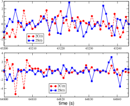
Figure 9: For $\epsilon_{v}$ as in Eq.(58) and $\chi=2$, we report in units $10^{-15}$ two typical sets of 45 seconds for the two functions $2C(t)$ and $2S(t)$ of Eq.(76). The two sets belong to the same random sequence and refer to two sidereal times that differ by 6 hours. The boundaries of the stochastic velocity components Eqs.(85) and (86) are controlled by $(V,\alpha,\gamma)_{\rm CMB}$ through Eqs.(79) and (89). For a laser frequency of $2.8\cdot 10^{14}$ Hz, the range $\pm 3.5\cdot 10^{-15}$ corresponds to a typical frequency shift $\Delta\nu$ in the range $\pm 1$ Hz, as in our Fig.5.

To understand how radical is the modification produced by Eqs.(91), we recall the traditional procedure adopted in the classical experiments. One was measuring the fringe shifts at some given sidereal time on consecutive days so that changes of the orbital velocity were negligible. Then, see Eqs.(49) and (76), the measured shifts at the various angle $\theta$ were averaged

$$\langle{{\Delta\lambda(\theta;t)}\over{\lambda}}\rangle_{\rm stat}={{2D}\over{\lambda}}\left[2\sin 2\theta~{}\langle S(t)\rangle_{\rm stat}+2\cos 2\theta~{}\langle C(t)\rangle_{\rm stat}\right]$$ (92)

and finally these average values were compared with models for the Earth cosmic motion.

However if the signal is so irregular that, by increasing the number of measurements, $\langle C(t)\rangle_{\rm stat}\to 0$ and $\langle S(t)\rangle_{\rm stat}\to 0$ the averages Eq.(92) would have no meaning. In fact, these averages would be non vanishing just because the statistics is finite. In particular, the direction $\theta_{0}(t)$ of the drift (defined by the relation $\tan 2\theta_{0}(t)=S(t)/C(t)$) would vary randomly with no definite limit.

This is why one should concentrate the analysis on the 2nd-harmonic amplitudes

$$A_{2}(t)={{2D}\over{\lambda}}~{}2\sqrt{S^{2}(t)+C^{2}(t)}\sim{{2D}\over{\lambda}}~{}\epsilon{{v^{2}_{x}(t)+v^{2}_{y}(t)}\over{c^{2}}}$$ (93)

which are positive-definite and remain non-zero under the averaging procedure. Moreover, these are rotational-invariant quantities and their statistical average

$$\langle A_{2}(t)\rangle_{\rm stat}\sim{{2D}\over{\lambda}}\cdot{{\pi^{2}}\over{18}}\cdot\epsilon\cdot\frac{V^{2}\sin^{2}z(t)}{c^{2}}$$ (94)

would remain unchanged in the isotropic model Eq.(89) or with the alternative choice $d_{x}(t)\equiv\tilde{v}_{x}(t)$ and $d_{y}(t)\equiv\tilde{v}_{y}(t)$.

Analogous considerations hold for the modern experiments where $\frac{\Delta\bar{c}_{\theta}(t)}{c}$ is extracted from the frequency shift of two optical resonators. Again, the $C(t)$ and $S(t)$ obtained, through Eq.(76), from the very irregular signal (see e.g. Fig.5), are compared with the slowly varying parameterizations Eqs.(82) and (83). No surprise that the average values $(C_{k})^{\rm avg}=0$, $(S_{k})^{\rm avg}=0$ of the resulting Fourier coefficients become smaller and smaller by simply increasing the number of observations. To appreciate the change of perspective in our stochastic model, compare with a simulation of the $C(t)$ and $S(t)$ in Fig.9.

References

- [1] S. Weinberg, The Trouble with Quantum Mechanics, The New York Review of Books, January 19, 2017.
- [2] Ph. Blanchard, J. Fröhlich, and B. Schubnel, A “garden of forking paths” - The quantum mechanics of histories of events Nucl. Phys. B 912 (2016) 463; arXiv:1603.09664 [quant-ph].
- [3] A. Einstein, B. Podolski and N. Rosen, Can quantum-mechanical description of physical reality be considered complete?, Phys. Rev.47 (1935) 777.
- [4] Full reference to all papers by J. S. Bell, can be found in the Volume Collection, Speakable and Unspeakable in Quantum Mechanics, 2nd edition, Cambridge University Press, 2004.
- [5] H. P. Stapp, A Bell-type theorem without hidden variables, Am. Journ. of Physics, 72 (2004) 30.
- [6] A. Shimony, An Analysis of Stapp’s “A Bell-type theorem without hidden variables”, arXiv:quant-ph/0404121.
- [7] J. Bricmont, What Did Bell Really Prove?, in Quantum NonLocality And Reality, 50 Years of Bell’s theorem, M. Bell and S. Gao. Eds. Cambridge Univ. Press 2016, p. 49.
- [8] T. Maudlin, Quantum Non-Locality and Relativity, Blackwell, Cambridge, 2011.
- [9] P. A. M. Dirac, Development of the Physicist’s Conception of Nature, in The Physicist’s Conception of Nature, J. Mehra Ed., Reidel, Boston 1973.
- [10] S. Weinberg, Gravitation and Cosmology, John Wiley and Sons, Inc., 1972, pag. 52.
- [11] D. Bohm and B. Hiley, The Undivided Universe, Routledge, London 1993.
- [12] L. Hardy, Quantum mechanics, local realistic theories, and Lorentz-invariant realistic theories, Phys. Rev. Lett. 68 (1992) 2981.
- [13] P. Caban and J. Rembielinski, Lorentz-covariant quantum mechanics and preferred frame, Phys. Rev. A59 (1999) 4187.
- [14] S. Liberati, S. Sonego and M. Visser, Faster-than-c signals, special relativity, and causality, Ann. Phys.298 (2002) 167.
- [15] P. H. Eberhard, Bell’s Theorem and the Different Concept of Locality, Nuovo Cim.B 46 (1978) 392.
- [16] P. H. Eberhard, A realistic model for Quantum Theory with a locality property, in Quantum Theories and Pictures of Reality, W. Schommers Ed., Springer Verlag, Berlin (1989), p.169.
- [17] R. Garisto, What is the speed of quantum information?, arXiv:quant-ph/0212078.
- [18] M. Yoon and D. Huterer, Kinematic Dipole Detection With Galaxy Surveys: Forecasts And Requirements, Astrophys. J. Lett. 813 (2015) L18.
- [19] V. Scarani, W. Tittel, H. Zbinden and N. Gisin, The speed of quantum information and the preferred frame: analysis of experimental data, Phys. Lett. A 276 (2000) 1.
- [20] B. Cocciaro, S. Faetti and L. Fronzoni, A lower bound for the velocity of quantum communication in the preferred frame, Phys. Lett. A375 (2011) 379.
- [21] D. Salart, A. Baas, C. Branciard, N. Gisin and H. Zbinden, Testing spooky action at a distance, Nature 454 (2008) 861.
- [22] J.-D. Bancal, S. Pironio, A. Acin, Y.-C. Liang, V. Scarani, and N. Gisin, Quantum nonlocality based on finite-speed causal influences leads to superluminal signaling, Nature Physics 8 (2012) 867.
- [23] B. Cocciaro, S. Faetti and L. Fronzoni, Fast measurements of entanglement over a kilometric distance to test superluminal models of Quantum Mechanics: final results , J. Phys. Conf. Ser. 1275 (2019) 012035.
- [24] L. Maiani and M. Testa, Causality in quantum field theory, Phys. Lett. B356 (1995) 319.
- [25] J. Bricmont, Making Sense of Quantum Mechanics, Springer Int. Publ. 2016.
- [26] G. ’t Hooft, Search of the Ultimate Building Blocks, Cambridge Univ. Press 1997, p.70.
- [27] M. Consoli, P.M. Stevenson, Physical mechanisms generating spontaneous symmetry breaking and a hierarchy of scales, Int. J. Mod. Phys. A 15(2000) 133, hep-ph/9905427.
- [28] L. Kostro, Einstein and the Ether, Italian translation, Ed. Dedalo, Bari 2001.
- [29] R. Y. Chiao, Conceptual tensions between quantum mechanics and general relativity: Are there experimental consequences?, in “Science and Ultimate Reality: From Quantum to Cosmos”, honoring John Wheeler’s 90th birthday. J. D. Barrow, P. C. W. Davies, and C. L. Harper eds. Cambridge University Press (2003); arXiv:gr-qc/0303100.
- [30] J. M. Jauch and K. M. Watson, Phenomenological Quantum-Electrodynamics, Phys. Rev. 74, 950 (1948).
- [31] M. Consoli, C. Matheson and A. Pluchino, The classical ether-drift experiments: a modern re-interpretation Eur. Phys. J. Plus, 128 (2013) 71.
- [32] M. Consoli and A. Pluchino, Cosmic Microwave Background and the issue of a fundamental preferred frame, Eur. Phys. Jour. Plus 133 (2018) 295.
- [33] M. Consoli and A. Pluchino, Michelson-Morley Experiments: an Enigma for Physics and the History of Science, World Scientific 2019, ISBN 978-981-3278-18-9.
- [34] M. Consoli and A. Pluchino, CMB, preferred reference system and dragging of light in the earth’s frame, Universe 7 (2021) 311;arXiv:2109.03047 [physics.gen-ph].
- [35] M. Consoli, A. Pluchino and A. Rapisarda, Cosmic Background Radiation and ‘ether-drift’ experiments, Europhysics Lett. 113 (2016) 19001.
- [36] S.R. Coleman, E.J. Weinberg, Radiative Corrections as the Origin of Spontaneous Symmetry Breaking, Phys. Rev. D7 (1973) 1888.
- [37] P.H. Lundow, K. Markström, Critical behavior of the Ising model on the four-dimensional cubic lattice, Physical Review E 80 (2009) 031104.
- [38] P.H. Lundow, K. Markström, Non-vanishing boundary effects and quasi-first order phase transitions in high dimensional Ising models, Nucl. Phys. B845 (2011) 120.
- [39] S. Akiyama, Y. Kuramashi, T. Yamashita, Y. Yoshimura, Phase transition of four-dimensional Ising model with higher-order tensor renormalization group, Phys. Rev. D 100 (2019) 054510.
- [40] See, for instance, R. F. Streater and A. S. Wightman, PCT, Spin and Statistics, and all that, W. A. Benjamin, New York 1964.
- [41] I.E. Segal, Is the Physical Vacuum Really Lorentz-Invariant?, in Differential Geometry, Group Representations, and Quantization, J.D. Hennig, W.Lücke, J. Tolar, Eds. Lecture Notes in Physics Vol. 379, Springer 1991.
- [42] E. V. Stefanovich, Is Minkowski Space-Time Compatible with Quantum Mechanics?, Found. Phys.32 (2002) 673.
- [43] S. D. Glazek and T. Maslowski, Renormalized Poincaré algebra for effective particles in quantum field theory Phys. Rev. D65 (2002) 065011.
- [44] M. Consoli and A. Ciancitto, Indications of the occurrence of spontaneous symmetry breaking in massless theory, Nucl. Phys. B254, 653 (1985).
- [45] S. Weinberg, The Quantum Theory of Fields, Cambridge University Press, Vol.II, pp. 163-167.
- [46] M. Consoli and E. Costanzo, Is the physical vacuum a preferred frame?, Eur. Phys. Journ. C54 (2008) 285.
- [47] M. Consoli and E. Costanzo, Precision tests with a new class of dedicated ether-drift experiments, Eur. Phys. Journ. C55 (2008) 469.
- [48] M. Consoli,Probing the vacuum of particle physics with precise laser interferometry, Found. of Phys. 45, 22 (2015).
- [49] M. Consoli,On the low-energy spectrum of spontaneously broken theories , Mod. Phys. Lett. A 26 (2011) 531.
- [50] Y. B. Zeldovich, The Cosmological constant and the theory of elementary particles, Sov. Phys. Usp. 11, 381 (1968).
- [51] S. Weinberg, The cosmological constant problem, Rev. Mod. Phys. 61, 1 (1989).
- [52] G. F. Smoot, Cosmic microwave background radiation anisotropies: Their discovery and utilization, Nobel Lecture, Rev. Mod. Phys. 79, 1349 (2007).
- [53] A. Ungar,The relativistic composite-velocity reciprocity principle, Found. of Phys. 30, 331 (2000).
- [54] J. P. Costella et al.,The Thomas rotation, Am. J. Phys. 69, 837 (2001).
- [55] K. O’ Donnell and M. Visser,Elementary analysis of the special relativistic combination of velocities, Wigner rotation, and Thomas precession, Eur. J. Phys. 32, 1033 (2011).
- [56] M. Nagel et al., Direct terrestrial test of Lorentz symmetry in electrodynamics to , Nature Comm.6, 8174 (2015).
- [57] A. A. Michelson and E. W. Morley, On the Relative Motion of the Earth and the Luminiferous Ether, Am. J. Sci. 34, 333 (1887).
- [58] D. C. Miller, The Ether-Drift Experiment and the Determination of the Absolute Motion of the Earth, Rev. Mod. Phys. 5, 203 (1933).
- [59] A. A. Michelson, et al., Conference on the Ether-Drift Experiments, Ap. J. 68 (1928) p. 341-402.
- [60] K. K. Illingworth, A Repetition of the Michelson-Morley Experiment Using Kennedy’s Refinement, Phys. Rev. 30, 692 (1927).
- [61] R. Tomaschek, About the Michelson experiment with fixed star light, Astron. Nachrichten, 219, 301 (1923), English translation.
- [62] A. Piccard and E. Stahel, REALIZATION OF THE EXPERIMENT OF MICHELSON IN BALLOON AND ON DRY LAND, Journ. de Physique et Le Radium IX (1928) No.2.
- [63] A. A. Michelson, F. G. Pease and F. Pearson,Repetition of the Michelson-Morley Experiment, Nature, 123, 88 (1929).
- [64] A. A. Michelson, F. G. Pease and F. Pearson, Repetition of the Michelson-Morley experiment, J. Opt. Soc. Am. 18, 181 (1929).
- [65] F. G. Pease, Ether-Drift Data, Publ. of the Astr. Soc. of the Pacific, XLII, 197 (1930).
- [66] G. Joos, Die Jenaer Wiederholung des Michelsonversuchs, Ann. d. Physik 7, 385 (1930).
- [67] R. J. Kennedy,Simplified theory of the Michelson-Morley experiment, Phys. Rev. 47, 965 (1935).
- [68] J. C. Maxwell, Ether, Encyclopaedia Britannica, 9th Edition, 1878.
- [69] M. Consoli, A. Pluchino and A. Rapisarda,Basic randomness of nature and ether-drift experiments, Chaos, Solitons and Fractals 44, 1089 (2011).
- [70] M. Consoli, A. Pluchino, A. Rapisarda and S. Tudisco, The vacuum as a form of turbulent fluid: motivations, experiments, implications, Physica A394, 61 (2014).
- [71] E. T. Whittaker,A History of the Theories of Aether and Electricity, Dover Publ., New York 1989.
- [72] O. V. Troshkin, On wave properties of an incompressible turbulent fluid, Physica A 168 (1990) 881.
- [73] H. E. Puthoff,Linearized turbulent flow as an analog model for linearized General Relativity, arXiv:0808.3401 [physics.gen-ph].
- [74] T. D. Tsankov,Classical Electrodynamics and the Turbulent Aether Hypothesis, Preprint February 2009, unpublished.
- [75] L. A. Saul, Spin Waves as Metric in a Kinetic Space-Time, Phys. Lett. A 314 (2003) 472.
- [76] M. Consoli, A kinetic basis for space-time symmetries, Phys. Lett. A376 (2012) 3377.
- [77] E. Nelson, A derivation of the Schrödinger Equation from Newtonian Mechanics, Phys. Rev. 150 (1966) 1079.
- [78] P. Jizba and H. Kleinert, Superstatistics approach to path integral for a relativistic particle Phys. Rev. D 82 (2010) 085016.
- [79] P. Jizba, F. Scardigli, Special Relativity induced by Granular Space, Eur. Phys. J. C73 (2013) 2491.
- [80] R. P. Feynman, R. B. Leighton and M. Sands, The Feynman Lectures on Physics, Addison Wesley Publ. Co. 1963.
- [81] L. Onsager, N. Cimento, Statistical hydrodynamics, Suppl. 6, 279 (1949).
- [82] G. L. Eyink and K. R. Sreenivasan, Onsager and the theory of hydrodynamic turbulence, Rev. Mod. Phys. 78, 87 (2006).
- [83] J. J. Nassau and P. M. Morse,A Study of Solar Motion by Harmonic Analysis, Ap. J. 65, 73 (1927).
- [84] L. D. Landau and E. M. Lifshitz,Fluid Mechanics, Pergamon Press 1959.
- [85] J. C. H. Fung et al., Kinematic simulation of homogeneous turbulence by unsteady random Fourier modes, J. Fluid Mech. 236, 281 (1992).
- [86] R. S. Shankland et al., New Analysis of the Interferometer Observations of Dayton C. Miller, Rev. Mod. Phys.27, 167 (1955).
- [87] L. S. Swenson Jr., The Ethereal Aether, A History of the Michelson-Morley-Miller Aether-Drift Experiments, 1880-1930. University of Texas Press, Austin 1972.
- [88] Loyd S. Swenson Jr.,The Michelson-Morley-Miller Experiments before and after 1905, Journ. for the History of Astronomy, 1, 56 (1970).
- [89] J. Shamir and R. Fox, A New Experimental Test of Special Relativity, N. Cim. 62B, 258 (1969).
- [90] G. Joos, Note on the Repetition of the Michelson-Morley Experiment, Phys. Rev. 45, 114 (1934).
- [91] D. C. Miller, Comments on Dr. Georg Joos’s Criticism of the Ether-Drift Experiment, Phys. Rev. 45 (1934) 114.
- [92] E. R. Farkas and W. W. Webb, Precise and millidegree stable control for fluorescense imaging, Rev. Scient. Instr. 81, 093704 (2010).
- [93] Y. Zhao, D. L. Trumper, R. K. Heilmann, M. L. Schattenburg, Optimizatiom and temperature mapping of an ultra-high thermal stability enviromental enclosure, Precision Engin. 34, 164 (2010).
- [94] I. P. Prikhodko, A. A. Trusov, A. M. Shkel, Compensation of drifts in high-Q MEMS gyroscopes using temperature self-sensing, Sensors and Actuators A 201, 517 (2013).
- [95] H. Müller, et al. , Modern Michelson-Morley Experiment using Cryogenic Optical Resonators, Phys. Rev. Lett. 91, 020401 (2003).
- [96] Ch. Eisele, M. Okhapkin, A. Nevsky, S. Schiller, A crossed optical cavities apparatus for a precision test of the isotropy of light propagation, Opt. Comm. 281, 1189 (2008).
- [97] S. Herrmann, et al., Rotating optical cavity experiment testing Lorentz invariance at the level, Phys.Rev. D 80, 10511 (2009).
- [98] Ch. Eisele, A. Newsky and S. Schiller, Laboratory Test of the Isotropy of Light Propagation at the Level, Phys. Rev. Lett. 103, 090401 (2009).
- [99] M. Nagel et al.,Ultra-stable Cryogenic Optical Resonators For Tests Of Fundamental Physics, arXiv:1308.5582[physics.optics].
- [100] Q. Chen, E. Magoulakis, and S. Schiller,High-sensitivity crossed-resonator laser apparatus for improved tests of Lorentz invariance and of space-time fluctuations, Phys. Rev. D 93 , 022003 (2016).
- [101] K. Numata, A, Kemery and J. Camp, Thermal-Noise Limit in the Frequency Stabilization of Lasers with Rigid Cavities, Phys. Rev. Lett. 93, 250602 (2004).
- [102] H. Müller, et al., Precision test of the isotropy of light propagation, Appl. Phys. B 77, 719 (2003).
- [103] M. Consoli and L. Pappalardo, Emergent gravity and ether-drift experiments, Gen. Rel. and Grav. 42, 2585 (2010).
- [104] J. Broekaert, A Spatially-VSL Gravity Model with 1-PN limit of GRT, Found. of Phys. 38, 409 (2008).
- [105] A. S. Eddington,Space, Time and Gravitation, Cambridge University Press, 1920.
- [106] L. D. Landau and E. M. Lifshitz,The Classical Theory of Fields, Pergamon Press, 1971, p.257.
- [107] C. Lämmerzahl et al., OPTIS: a satellite-based test of special and general relativity,Class. Quantum Gravity 18, 2499 (2001).
- [108] D. A. Kirzhnits and V. L. Polyachenko, ON THE POSSIBILITY OF MACROSCOPIC MANIFESTATIONS OF VIOLATION OF MICROSCOPIC CAUSALITY, Sov. Phys. JETP 19, 514 (1964).
- [109] S. A. Bludman and M. A. Ruderman, Possibility of the Speed of Sound Exceeding the Speed of Light in Ultradense Matter, Phys. Rev. 170, 1176 (1968).
- [110] M. Ruderman, Causes of Sound Faster than Light in Classical Models of Ultradense Matter, Phys. Rev. 172, 1286 (1968).
- [111] S. A. Bludman and M. A. Ruderman, Noncausality and Instability in Ultradense Matter, Phys. Rev. D1, 3243 (1970).
- [112] B. D. Keister and W. N. Polyzou, Causality in dense matter, Phys. Rev. C54, 2023 (1996).
- [113] P. M. Stevenson, How do sound waves in a Bose-Einstein condensate move so fast?, Phys. Rev. A68 (2003) 055601.
- [114] P. M. Stevenson, HYDRODYNAMICS OF THE VACUUM, Int. J. Mod. Phys. A 21, 2877 (2006).
- [115] P. M. Stevenson, Are There Pressure Waves in the Vacuum?, in Proceedings of the Second Meeting on CPT and Lorentz Symmetry, V. A. Kostelecky Ed., World Scientific, Singapore, 2002; arXiv:hep-ph/0109204.
- [116] P. Zizzi, Quantum Holography from Fermion Fields, Quantum Rep. 2021, 3(3), 576-591; https://doi.org/10.3390/quantum3030037.
- [117] P. Zizzi, Consciousness and logic in a quantum computing universe, in ”The emerging physics of consciousness”, Jack Tuszynski Ed., Springer, 2006.