New dipole instabilities in spherical stellar systems

Abstract

Spherical stellar systems have weakly-damped response modes. The dipole modes are seiche modes. The quadrupole are zero pattern-speed prolate modes, the stable precursors to the radial-orbit instability (ROI). We demonstrate that small wiggles in the distribution function (DF) can destabilise the dipole modes and describe the newly identified instabilities in NFW-like dark-matter (DM) halos and other power-law spherical systems. The modes were identified in N-body simulations using multivariate singular spectrum analysis (MSSA) and corroborated using linear-response theory. The new mode peaks inside the half-mass radius but has a pattern speed typical of an outer-halo orbit. As it grows, the radial angle of the eccentric orbits that make up the mode correlate and lose angular momentum by a resonant couple to outer-halo orbits. This leads to an unsteady pattern with a density enhancement that swings from one side of the halo to another along a diameter, like the orbits that comprise the instability. In this way, the dipole mode is similar to the ROI. Since the DF found in Nature is unlikely to be smooth and isotropic with $df(E)/dE<0$ necessary for Antonov stability, these modes may be ubiquitous albeit slowly growing. Halos that are less extended than NFW, such as the Hernquist model, tend to be stable to this dipole instability. We present the critical stability exponents for one- and two-power models. These different critical outer power-law exponents illustrate that the gravitational coupling between the inner and outer DM halo depends on the global shape of density profile.

1 Introduction

1.1 Instabilities in spherical stellar systems

The stability of spherical stellar systems are the best well-studied of all astronomical equilibrium models. The modern contributions began with work of Antonov (1962, 1973). Since then, there have been three main approaches: the study of global functionals of energy following Antonov’s approach, the analytic derivation of discrete modes, and numerical simulation. The early work on the modal approach is summarised in the monographs by Fridman & Polyachenko (1984a) and followed up by Palmer & Papaloizou (1987); Weinberg (1991); Palmer (1994). In brief, one simultaneously linearises and solves the collisionless Boltzmann equation and the Poisson equation. With a careful choice of phase-space variables and Fourier decomposition, we obtain a solvable set of algebraic equations for the frequency spectrum. Using this dispersion relation for the eigenfrequencies of the system, an instability is present if at least one of the eigenfrequencies has a non-zero positive imaginary part, while stability holds if they are all real or have negative imaginary parts. The set of stable models are candidates for describing long-lived astronomical systems, galaxies in particular. See Binney & Tremaine (2008) for a comprehensive review.

Beyond stability, environmental interactions and assembly history disturb equilibria. Like plasma systems, disturbances to a self gravitating systems can be described by linear operator on a function space with infinite degrees of freedom. Mathematically, such operators have a more complex spectrum than the familiar normal (eigen) modes of a finite system (e.g. Riesz & Nagy, 2012). As in plasmas, self-gravitating stellar systems have a spectrum of both continuous and point modes (Ichimaru, 1973; Ikeuchi, Nakamura & Takahara, 1974), and the response of an initially equilibrium system to a perturbation is a combination of both parts of the spectrum. The point modes have distinct shapes reinforced by their own gravity. In plasma physics, the modes in the point spectrum are called Landau modes (Landau, 1946) and those in the continuous spectrum are called van Kampen modes (van Kampen, 1955). The initial response in stellar systems is dominated by the continuous modes which typically phase mix in several dynamical times. The most commonly known point mode is the Jeans’ instability in a homogeneous sea of stars (e.g. Binney & Tremaine, 2008). See Lau & Binney (2021) for a discussion of van Kampen modes in the context of stellar dynamics.

This contribution concerns the long, slow evolution of a dark matter halo and therefore, the behaviour of point modes is key. The point modes continue to exist for stable systems but are damped rather than growing; i.e. their frequencies have negative imaginary parts. For example, the Jeans’ mode in the homogeneous system becomes a damped mode with increasing velocity dispersion. This mode can be excited by a disturbance and persist over time if the damping time is sufficient long. Weinberg (1994) extended this idea to spherical systems, demonstrating the existence of both $l=1$ and $l=2$ damped modes in two ways. First, a self-consistent solution of the linearised collisionless Boltzmann equation provides a response operator that defines damped and growing modes (often called the dispersion relation by analogy with plasma physics) and, second, by N-body simulation.

While early work on time-dependence of galaxy structure focused on stability and disc features, modern suites of numerical N-body simulations (Nelson et al., 2018; Monachesi et al., 2019; Dubois et al., 2021; Wetzel et al., 2022) make it clear that the evolution of galaxies are driven by disturbances from their assembly at early times and their environment in the current epoch. The fluctuations from environmental disturbances such as satellite encounters or Poisson noise from $N$-body distributions may excite these weakly self-gravitating features. Calculations for unstable evolutionary modes in galactic discs have found evidence for point modes supported in various analytic geometries (e.g. Fouvry et al., 2015; De Rijcke, Fouvry & Pichon, 2019).

1.2 Overall plan

While we can understand the basic governing principles with detailed mathematical models from Hamiltonian perturbation theory, the inter-component and environmental interactions that produce key features of galaxy morphology, such as bars and spiral arms, are hard if not impossible to study from dispersion relations alone. This paper was motivated by simulations of disc galaxies evolving in dark matter halos (e.g. Petersen, Weinberg & Katz, 2019a, b, c). In these papers, we performed controlled simulations using our basis-function expansion (BFE) Poisson solver (Petersen, Weinberg & Katz, 2021a, exp). The BFEs are designed to spatially best represent the degrees of freedom that we know to describe the collective nature of the dynamics. We noticed that $l=1$ power in the halo appeared quickly and persisted over the typically 8–10 Gyr of the simulation. These same BFE techniques underpin the numerical computation of the dispersion relations used in Weinberg (1991, 1994). We exploit this correspondence for additional insight.

More recently, Weinberg & Petersen (2021) combined the BFE representation of the possibly unknown dynamics in simulations with the knowledge acquisition algorithm known as multivariate singular spectrum analysis (mSSA, e.g. Ghil & Vautard, 1991; Golyandina, Nekrutkin & Zhigljavsky, 2001; M. Ghil et al., 2002). This allows us to find couplings that may be too hard to predict otherwise. A detailed investigation of the persistent $l=1$ halo power revealed the existence of response mode that slowly grows for a variety of plausibly realistic dark-matter halo conditions.

In short, the plan of the remainder is as follows. We begin with a description of methods and models in Section 2. We move on to a description of the new instability in Section 3. Section 4 characterises the instability in detail using the combination of BFE representation and mSSA. This helps determine the nature of the mode and its physical mechanism. We verify that the unstable mode is not code dependent in Section 5 by recovering the results of our exp simulations using gadget-2. Section 6 demonstrates that the domain of instability found in the N-body simulations is predicted by the linear perturbation theory and corroborates the empirical findings of the previous sections. We end with some final discussion and a summary in Section 7.

2 Simulations and methods

We review the key features of exp (Sec. 2.1), mSSA (Sec. 2.2), and linear response theory (Sec. 2.3) followed by a description of the model families used in this investigation (Sec. 2.4).

2.1 N-body methods

We require a description of the potential and force vector at all points in physical space and time to compute the time evolution for an N-body system. We accomplish this using a biorthogonal basis set of density-potential pairs that solve the Poisson equation. We generate density-potential pairs using the basis function expansion (BFE) algorithm described in Weinberg (1999) and implemented in exp. In the BFE method (Clutton-Brock, 1972, 1973; Hernquist & Ostriker, 1992), a system of biorthogonal potential-density pairs are calculated and used to approximate the potential and force fields in the system. The functions are calculated by numerically solving the Sturm-Liouville equation for eigenfunctions of the Laplacian. The full method is described precisely in Petersen, Weinberg & Katz (2021b). Appendix A provides technical details and a presentation of simulation parameters.

For comparison, we also use gadget-2 (Springel, 2005) which computes gravitational forces with a hierarchical tree algorithm. We only need the tree-gravity part of gadget-2 to follow the evolution of a self-gravitating collisionless N-body system. We choose gadget-2 because it is well-known in the community but any modern gravity-only Lagrangian code would suffice. We compute the softening following the algorithm from Dehnen (2001). In practice, gadget-2 does not conserve linear momentum as well as exp, and this demands a recentring computation for inter-comparison. The density centre for the snapshots produced by each code is evaluated using kd-tree nearest-neighbour estimator. The density and potential fields for the evolved phase space for each code are then computing using the same BFE expansion used by exp.

2.2 Multivariate Singular Spectrum Analysis

Singular spectrum analysis (SSA, see Golyandina, Nekrutkin & Zhigljavsky, 2001) extracts correlated signals from a time series by analysing the covariance matrix of a series at successive times lags with itself. For example, consider a pure sinusoidal signal. When the lag equals the period, the corresponding cross-covariance element will be large, otherwise it will tend to vanish by interference. This method works for aperiodic signals as well. For a time series with some arbitrary but coherently varying signal, its correlated temporal variations will reinforce when the lag coincides with its natural time scale. SSA has similarities with its cousin, PCA (principal component analysis). In PCA, the typical covariance matrix consists of a single field variable observed at multiple positions. In SSA, the covariance matrix consists of a single time series observed in different time windows; the resulting components derived through SSA are temporal principal components.

The BFE coefficients for an N-body simulation at any point in time (see Appendix A) are a spatial analysis of the gravitational field. The full simulation is represented by multiple time series, one for each coefficient. The entire BFE in time encodes a time-varying interrelated spatial structure. To apply SSA to this situation, we extend the analysis of a single time series to multiple time series simultaneously; this is mSSA and the application to dynamics is described in Weinberg & Petersen (2021); Johnson et al. (2023). In short, mSSA applied to a BFE in time provides a combined spatial and temporal spectral analysis. The dominant eigenvectors reveal key correlated dynamical signals in our simulation. The analyses of simulations in Section 3 rely on mSSA for isolating correlated dynamical signals.

2.3 Linear response theory

We use the matrix-method solution of the linearised collisionless Boltzmann equation to estimate the location of the point modes to guide our interpretation of the N-body simulations. This semi-numerical method has been used by the author and many others (op. cit., Sec. 1) to explore secular evolution. In short, this method discretises the variation in the density and potential fields under a Hamiltonian flow by expanding them in biorthogonal potential–density functions that mutually solve the Poisson equation. With this built-in solution to the Poisson equation, the response of the Hamiltonian system to an applied perturbation may be derived by splitting the slower temporal evolution driven by the perturbation from the faster characteristic orbital times, and then averaging over these latter degrees of freedom. This method can be used to estimate the evolution of galactic system to a wide variety of distortions such as minor mergers and predict the features of disc and halo interactions. Here, we are interested the answer to a very specific question: under what condition is the output response of the system the same as the input perturbation? This is a generalised eigenvalue problem and the solutions are the point modes described earlier. The complex frequency $\omega$ that satisfies this condition determines whether this response grows ($\Re(\omega)>0$) or decays ($\Re(\omega)<0$). More details on computing this eigenvalue problem and finding the shape of the shape of the mode can be found in Appendix B.

2.4 Models

Nearly all of idealised dark-matter halo models have infinite extent and some have infinite mass. Their isotropic phase-space distribution functions, $f(E)$, have $df/dE<0$ everywhere and are stable by Antonov’s theorems (op. cit.). This idealisation does not describe the true structure of a halo, however. By their nature, halos will have varying anisotropy, dark-matter density floors (Diemer & Kravtsov, 2014) and presumably, ‘bumps’ and ‘wiggles’ in their distribution owing to incomplete mixing from assembly and mergers. We will demonstrate that these types of deviations at specific scales drive growth of otherwise damped modes.

Our fiducial model is NFW-like (Navarro, Frenk & White, 1997) with $c=10$ and an outer truncation to provide finite mass. Although this is a smaller concentration than a cosmological dark-matter halo with the Milky Way mass, this concentration provides a good match to the Milky Way rotation curve when combined with a realistic Milky Way disc (McMillan, 2017; Petersen, 2020). The NFW halo is slightly modified at small radii and large radii, to account for dissipation and evolution at small radii and provide a finite mass at large radii. We adopt:

$$\rho(r)\propto\frac{1}{r+r_{c}}\frac{1}{(r+r_{a})^{2}}{\cal T}(r;r_{t},\sigma_{t})$$ (1)

where $r_{c}$ is the inner core radius, $r_{a}$ is the characteristic scale radius, $r_{t}$ is the outer truncation radius, and $\sigma_{t}$ is the truncation width. The truncation function, ${\cal T}$, is unity at radii $r\ll r_{t}$ and tapers the density to zero beyond $r_{t}$ with a width $\sigma_{t}$ as follows:

$${\cal T}(r;r_{t},\sigma_{t})=\frac{1}{2}\left[1-\mathop{\rm erf}\nolimits\left(\frac{r-r_{t}}{\sigma_{t}}\right)\right].$$ (2)

Here, the inner core radius is a convenience that obviates computing very high frequency orbits for a negligible measure of phase space when performing numerical dispersion relations from linear theory (Sec. 6 and App. B). We choose $r_{c}$ smaller than any scale of interest and, therefore, the value of $r_{c}$ has very little effect on the N-body simulations or the dispersion relation. We also study models from the more general two-power form inspired by the NFW model:

$$\rho(r)\propto\frac{1}{(r+r_{c})^{\alpha}}\frac{1}{(r+r_{a})^{\beta}}{\cal T}(r;r_{t},\sigma_{t})$$ (3)

For dark-matter-inspired models, we assign $\alpha=1$ and $\beta\in[2-4]$. The Hernquist (1990) model, for example, has $\alpha=1,\beta=3,r_{t}=\infty$. We also consider truncated single power-law models with $\alpha\in[1-3]$ and $\beta=0$.

We adopt virial units with unit mass and unit radius corresponding to the virial mass and virial radius, respectively, with $G=1$. In these units, our fiducial model has the parameters: $r_{c}=10^{-5},r_{a}=10^{-1},r_{t}=1.2,\sigma_{t}=0.1$. The fiducial simulations use $N=2\times 10^{7}$ particles. Some auxiliary tests use $N=10^{6},10^{7},10^{8}$. The main results are robust to the choice of $N$ in this range. Larger particle numbers better discern phase-space details.

For each model, we construct a phase-space distribution function in energy $E$ and angular momentum $L$ using the Osipkov-Merritt generalisation of the Eddington inversion (Osipkov, 1979; Merritt, 1985; Binney & Tremaine, 2008). We use a negative energy convention; the energies at the centre of the model are smallest (most bound) and are largest at the truncation radius (least bound). This generalisation assumes a univariate distribution function $f(Q)=f(E+L^{2}/2r_{q}^{2})$ where $L$ is the total angular momentum and $r_{q}$ is the anisotropy radius. For $r_{q}\rightarrow\infty,f(Q)\rightarrow f(E)$. We do not consider the more limited circularly anisotropic case, $f(Q)=f(E-L^{2}/2r_{q}^{2})$. In many cases, we use the pure Eddington method for an isotropic distribution function $f=f(E)$. We realise a phase-space point by first selecting random variates in energy $E$ and angular momentum $L$ by the acceptance-rejection technique from the distribution $f(Q)$. Then, the orientation of the orbital plane and the radial phase of the orbit are chosen by uniform variates from their respective ranges. This determines position and velocity. Particle masses are identical. The inversion is not guaranteed to provide physical solutions, and we restrict the models to parameters values that yield positive mass densities. We explore a suite of varying $r_{q}$ for the NFW-like model described by equation (1).

3 Key findings

Figure 1: The amplitude for harmonic orders $l=0,\ldots,4$. This amplitude, which is the square root of the gravitational power, is plotted for an easy comparison with the background. The $l=0$ amplitude contains the equilibrium field and is nearly constant in time. The $l=1$ amplitude is amplified by self gravity.

After running the primary simulation for approximately 7 virial time units (or 14 Gyr in Milky-Way time), the $l=1$ power is distinctly elevated. The gravitational power is computed directly from the biorthogonal expansion used to compute the N-body simulation as described in Appendix A. Figure 1 shows the power for each harmonic order from equation (7) for the primary simulation. The self-gravity in the weakly damped mode excited by the Poisson fluctuations elevates the power relative to the $l>1$ power. This is described in Weinberg (1994).

Then, we applied the mSSA technique to find the gravitationally correlated signal for $l=1$. Approximately 95% of the total variance are in the first three eigenvalues. A reconstruction of the field is shown in Figure 2. The scale of the feature coincides with characteristic scale of the NFW-like halo, $r_{a}$ (eq. 1), and its gravitational influence extends beyond the halo half-mass radius. Its shape is consistent with the weakly damped modes investigated in Weinberg (1994); Heggie, Breen & Varri (2020); Fouvry et al. (2021).

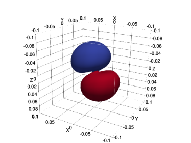
Figure 2: The mSSA reconstruction of the $l=1$ feature at $T=5$ or roughly at 10 Gyr in Milky-Way units. The isodensity surfaces illustrate the shape of the positive (red) and negative (blue) lobes of the dipole feature at the 10% level relative to the peak. The overdensity relative to the background equilibrium is 0.25% ($T=5$) at peak and this increases to 5% at late times.

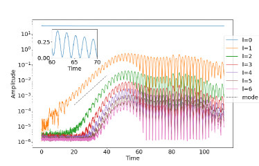
Figure 3: The amplitude for harmonic orders $l=0,\ldots,4$ for the same run as in Fig. 1 extended to $T=110$. The inset shows the periodicity in the $l=1$ power with a period of approximately 2 time units (or 4 Gyr in Milky-Way scaling). The amplitude of the $l=1$ mode relative to the background $l=0$ is approximately 10%. At late times, the low $l$ power aliases into higher order spherical harmonics will similar shape and trend to $l=4$ but successively lower amplitude. We have omitted $l>4$ curves for clarity. The exponential growth rate predicted by linear response theory (dashed line) reproduces that in the simulation.

Initially, the mode does not have a constant pattern speed but appears to be episodically fixed in space for several time units and then moves quickly to a new orientation. To investigate this strange and unexpected behaviour, we ran the simulation much further to $t\lesssim 100$ or approximately 30 Hubble times for Milky-Way scaling. The power plot for this extended run appears in Figure 3. Several key features are readily apparent:

1. mSSA reveals that the dominant mode at $T\lesssim 5$ is a damped mode with $\Re(\omega)\approx 3.2$. We confirm this with linear response theory in Section 6. This suggests the initial amplitude of this mode is the projection of the $l=1$ Poisson noise in the initial conditions. The amplitude of this mode slowly decays in time (see Sec. 4.1).

2. The unstable $l=1$ mode is present and exponentially growing from the beginning of the simulation. The real frequency of the growing mode is $\approx 1.9$. The early-time behaviour is obscured by blending with the noise-driven damped mode, but the growing mode has a clear, coherent pattern beginning at $T\approx 10$.

3. The $l=1$ power grows exponentially until $T\lesssim 40$.

4. Beyond this point, the $l=1$ power is approximately constant and perhaps slowly decaying for $T>40$.

5. The response shows a periodic modulation of approximately 2 time units (or 4 Gyr scaled to the Milky Way halo).

6. At early times, only the $l=1$ power increases but later, $T\gtrsim 20$, all harmonics begin to grow. This $l>1$ power results from the non-linear saturation of the initially dipole-only mode aliased into higher-order harmonics. There is no evidence from the mSSA analysis for new instabilities with $l>1$.

While surprising, this is not in violation of the Antonov stability criterion. The infinite-extent two-power NFW profile has $df(E)/dE<0$ but the truncated density distribution in equation (1) does not. The left-hand panel in Figure 4 shows the density profile from equation (1) with width $\sigma_{t}=n/10$ and $r_{t}=1+3\sigma_{t}$ for $n=1,\ldots,7$. The right-hand panels in this figure show the isotropic DF from the Eddington inversion. The lower right-hand side panel is a zoom in of the bump in the DF induced by the truncation ${\cal T}$. The truncation radius, $r_{t}$, give rise to a new energy scale, $E_{t}$. This results in an inflection in the distribution function $f(E)$ for $E\sim E_{t}$. The change in the phase-space gradient near $E_{t}$ enables a feedback channel between the inner and outer halo that drives the instability (Sec. 4). Even though we create this new scale by radial truncation, a wide variety of natural processes in DM haloes, such as accretion and disruption of dark subhaloes and dwarf galaxies or incomplete mixing from the halo’s early assembly history, can introduce special scales that break the monotonic run in $f(E)$ and result in similar dynamics. In summary, we use truncation as a device to introduce a particular scale but expect the implications to be generic. For example, we demonstrate in Section 6 that anisotropy causes an inflection in the distribution function which also results in instability.

We speculate that the existence of weakly damped and weakly growing $l=1$ rather than $l>1$ modes has several related origins. First, the damping rate in the point modes tends to increase with harmonic order because higher harmonic order presents more opportunities for commensurabilities at higher frequencies. Secondly, the self-gravitating pattern formed from a group of slowly precessing eccentric orbits is anomalously low compared to the azimuthal orbital frequencies. It therefore couples weakly to surrounding phase space. Finally, the low $l=1$ modal frequency circumstantially coincides with the characteristic orbital frequency in the outer halo coinciding with the bump in the distribution function. This provides an opportunity for instability.

4 Analysis and explanation

4.1 Evidence for an $l=1$ instability from N-body simulations

The phase-space distribution for spherical systems with no preferred axis may be represented by two action variables, $(I_{1},I_{2})$. The radial action is $I_{1}$ and the orbital angular momentum is $I_{2}$. The third action, $I_{3}$, is the azimuthal component of the orbital angular momentum, $J_{z}$. Let the conjugate angles be $(w_{1},w_{2},w_{3})$. Alternatively, we may describe phase space by independent functions of the actions. Here, we use energy $E=E(I_{1},I_{2}),\kappa=I_{2}/J_{\mbox{\tiny max}}(E)$ where $J_{\mbox{\tiny max}}(E)$ is the angular momentum for the circular orbit with energy $E$. The variables $(E,\kappa)$ provide a convenient rectangular domain.

Figure 5 shows the change the distribution function in action space between between the time $T=0$ (initial) and time $T=10$, the beginning of exponential growth phase. To estimate the distribution function, we bin the actions on a $60\times 60$ grid in $(I_{1},I_{2})$ and normalise to unit mass and phase-space volume. We then compute the difference between the initial and final densities averaged over 8 separate simulation snapshots. This extra bit of averaging reduces the sampling noise. All harmonic orders of the response are represented, not only $l=1$, but the $l=1$ interaction dominates. The location of the primary low-order commensurabilities for $\Omega_{p}\approx 1.82$ and $\Omega_{p}\approx 3.21$ also are shown in Figure 5. These two point modes are identified by linear perturbation theory using the methods described in Section 6 and Appendix B). We will demonstrate below that these two frequencies correspond to the exponentially growing and first damped mode, respectively. We denote the commensurabilities by the pair of integers $(l_{1},l_{2})$ such that $l_{1}\Omega_{1}+l_{2}\Omega_{2}=\Omega_{p}$ where $\Omega_{1},\Omega_{2}$ are the radial and tangential frequencies, respectively. The resonance tracks in $I_{1},I_{2}$ appear as anti-diagonal loci, generally.

Figure 5 shows that the global response is dominated by the $(1,1)$ resonance. This is resonance overlaps the position of the inflection in the background distribution function and transports energy and angular momentum from the point modes to larger values. The prominent feature between $I_{1}\in[0,0.2],I_{2}\in[0.05,0.1]$ results from a damped mode rather than the growing mode. The damped mode couples through the $(1,-1)$ at early times shown in this figure. This mode also results in transport from lower to higher energy and angular momentum. At later times, this couple disappears as the damped mode fades. This mode may be excited by the slight disequilibrium of the initial conditions, by collective relaxation driven by particle noise, or perhaps both. Further precise identification of its origin is elusive. The disappearance of the damped mode at late times suggests an excitation by the initial disequilibrium. However, the growing mode changes the underlying structure of the distribution, and this could modify the dressed, collective response.

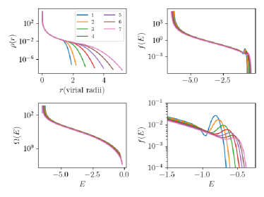
Figure 4: Upper left: the truncated density profile from eq. 1 for the truncation index $n$. Smaller index denotes sharper truncation. Lower left: the circular orbit frequency as function of energy for the same models. a Right: the isotropic distribution function, $f(E)$, for various truncation widths. The sharper the cut off, the larger the inflection in the run of $f(E)$. This bump in the tail of the distribution function powers the $l=1$ instability. The upper panel shows the full range of $f(E)$ and the lower panels zooms in on the bump.

Rather than employing linear response theory to investigate this intrinsically non-linear development, we use mSSA to explore the evolution empirically. The mSSA analysis applied to the $l=1$ time series of coefficients for our fiducial simulation provides a series of principal components in order of contribution to the temporal variance. While mSSA can approximate a signal with changing frequencies, it will also tend to separate signals of different frequencies into multiple PC pairs depending on the duration of the interval at a particular frequency. For example, imagine a time series that begins with a constant oscillation at frequency $\nu_{0}$, changes its frequency over a short period in the middle of series to a new frequency $\nu_{1}$ with $\nu_{1}\ll\nu_{0}$, followed by a constant oscillation at $\nu_{1}$ at late times. MSSA will provide two dominant PC pairs describing the early and late times with a third pair describing the transition. Conversely, mSSA will nicely separate a sinusoidally modulated chirp into to distinct PCs, one for the modulation and one for the chirp, as described in Weinberg & Petersen (2021). In summary, mSSA will separate punctuated signals into discrete intervals. Similarly, a DFT will characterise the frequency features in a PC but provide no information on where what time interval in the series dominates. So the two methods together are complementary. See Section 4.2 for an in-depth characterisation of the saturated mode using this approach.

For an example pertinent to the results of this and the next section, we apply mSSA to the $l=1$ coefficients in the same time interval, $T\in[0,12]$, used for Figure 4. Figure 6 describes the power from two low-order PCs pairs from $l=1$. The first pair (labeled ‘Pair 0’) describes most of the $l=1$ power in Figure 3. The third pair (labeled ‘Pair 2’) corresponds to the damped mode that dominates at early times. The frequency of peaks in each pair matches the the pattern speeds predicted by linear theory (see Sec. 6). Pair 1, not shown, is a blend of both frequencies. In summary, our application of mSSA to the N-body simulation recovers the main features of the expected linear development. However, we will see in the following sections that mSSA provides useful characterisation in the non-linear regime as well.

The power in the mSSA-derived PCs is power in the detrended, normalised coefficient time series. These DFT power spectra are not physical power in the gravitational field but the correlated temporal variation in the coefficient series about their detrended values. This detrending is motivated by the mathematics of SSA. The method will cleanly separate individual signals from a dynamical process that can be represented by a linear recurrence relation (see Golyandina, Nekrutkin & Zhigljavsky, 2001, Section 2.2 and Chapter 5). For example, exponential and trigonometric functions are exactly described by first- and second-order recurrences. The detrended BFE coefficient series look like zero-mean, unit-variance signals, and provide better separation; mSSA finds the growing, rotating mode clearly, isolating most of the feature in a pair of eigenvectors. For physical interpretation, we reconstruct these PCs into BFE coefficients. The amplitude of the coefficients for the same two PC pairs in Figure 6 is shown in Figure 7. This figure shows that the gravitational energy in Pair 0 from Figure 6 is exponentially growing and the power in Pair 2 is slowly decaying.

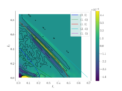
Figure 5: The change in the phase-space distribution function, $\Delta f(\mathbf{I})$, in radial actions and orbital angular momentum ($I_{1},I_{2}$) during the initial exponential growth phase. The zero-amplitude location of the primary commensurabilities with $l_{1}\Omega_{r}+l_{2}\Omega_{\phi}=\Omega_{p}$ are shown as colour coded curves labeled by $(l_{1},l_{2})$. Solid (dashed) lines correspond to $\Omega_{p}=1.82$ ($3.21$). These are the predicted pattern speeds of the growing (damped) modes. The large changes in $f(\mathbf{I})$ at small values of $(I_{1},I_{2})$ in the lower left-hand corner are distortions in the equilibrium model driven by the growing mode. The resonant couples advect orbits to larger $I_{1}$ and smaller $I_{2}$, primarily through the $(1,-1)$ resonance.

Figure 6: The DFT power from two dominant PC pairs from the mSSA analysis of $l=1$ coefficients with $n_{\mbox{\tiny max}}=12$. Only the low frequency part of the spectrum is shown; the power at larger $\nu$ decrease exponentially with increasing $\nu$. The dashed vertical lines show the real frequencies of the exponentially growing mode and first damped mode from linear response theory for comparison.

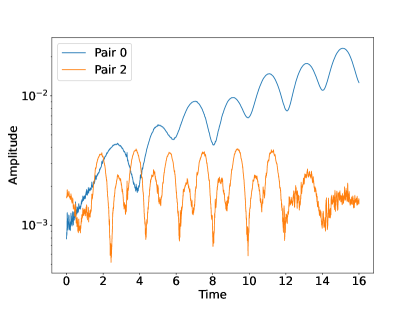
Figure 7: The coefficient amplitude (as in Fig. 1) from two dominant PC pairs from the mSSA analysis of $l=1$ coefficients with $n_{\mbox{\tiny max}}=12$.

4.2 The saturated mode

The exponential growth saturates at $T\approx 40$ (see Fig. 3) and the behaviour of the mode changes. The radial phase of participating eccentric orbits correlate, and the orbits sustaining the mode tend to bunch near apocentre. This is similar to the behaviour of the radial orbit instability: the precession angles bunch near apocentric angle yielding a quadrupole distortion. In this case, the orbits bunch in angle and oscillate in phase between pericentre and apocentre causing the modulation of the dipole power seen in Figure 3. The shape of the non-linear mode in these panels is similar to the early-time reconstruction in Figure 2. While the mode is sustained by the gravitational field of orbits strongly bunched in radial phase, the overall response of the halo is similar to the early-time feature which is only weakly bunched in phase.

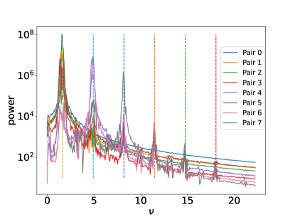
Figure 8: The DFT power of the first eight PC pairs for the mSSA analysis of the BFE coefficients beyond the saturation phase of the simulation (cf. Fig. 3). Here the dashed vertical lines show the odd frequency harmonics of the fundamental frequency with $\omega\approx 1.64$.

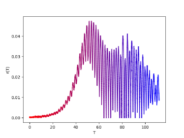
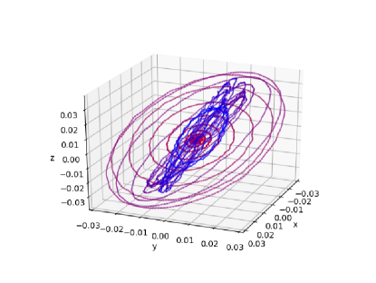
Figure 9: Top: the radial displacement of the cusp from the geometric centre of the halo as a function of time. Bottom: location of the peak density centre in three-dimensional space; time is colour coded as in the top panel. The orientation has been chosen roughly face-on to best illustrate trajectory of the cusp induced by the dipole mode. At early times ($T\lesssim 20$, we see oscillation with a uniform pattern speed with an slow outward spiral, consistent with the expected the linear behaviour of the mode. For $20\lesssim T\lesssim 40$, the non-linear bunching develops and the trajectory of the centre becomes more eccentric. For $T\gtrsim 40$, the trajectory becomes eccentric, the cusp begins to oscillate along a diameter.

The details of the transition from linear to non-linear are as follows. As the mode grows, its period increases. For the interval $T\in[0,10]$, one PC has the predicted frequency of the linear mode, $\Re(\omega)\approx 1.8$, and one has the faster damped-mode frequency, $\Re(\omega)\approx 2.5$ as described in Figure 6. At early times, e.g. the interval $T\in[0,5]$, the damped linear-mode frequency is dominant. As the interval increases from $T\in[0,20]$ to $T\in[0,40]$, the longer-period exponentially growing oscillation dominates. In the interval $T=[0,20]$, the first PC pair describes the exponentially growing mode with frequency $\Re(\omega)\approx 1.8$.

The DFT of the PCs for the larger interval, $T=[0,40]$ is shown in Figure 8. The peak in the same dominant PC pair becomes narrower and the initial damped-mode frequency is absent; the disturbance is nearly completely dominated by the non-linear mode for $T>20$. As the non-linear bunching in phase angle develops, the pattern speed slows to $\Re(\omega)\approx 1.6$. This suggests that the response mode begins close to the linear prediction: a constant pattern speed with exponential growth. As the amplitude increases and the disturbance becomes non-linear, the pattern becomes time dependent and shifts to a lower frequency typical of its nearly resonant orbits. If the mode were purely sinusoidal, the total power for the PC pairs would show only the slow change in overall amplitude. The strong modulation of the amplitude at late times in Figure 3 indicates that the mode’s oscillation behaviour is similar to that of a single nearly radial orbit consistent with bunching. Quantitatively, this results in strong odd harmonics of the primary frequency in the spectrum (Fig. 8). For comparison, the figure marks the location of the odd harmonics of fundamental frequency: $\omega\approx 1.64$.

At the same time, the gravitational potential from the dipole oscillation begins to affect the location of the inner cusp although the inner profile of the cusp itself remains intact. The internal dynamics of the cusp itself is decoupled from that of the mode but does provide a convenient diagnostic for the global effect of the dipole. The location of the cusp is depicted in Figure 9. At early times, the dipole rotates with a uniform pattern speed as expected from linear theory (see Sec. 6). Combined with the growth in amplitude, the trajectory of the cusp is an outward-moving spiral that follows the pattern of the linear mode. At later times, $T\gtrsim 40$, the cusp trajectory becomes increasingly radial along a diameter. This characterisation provides evidence that the saturated mode is an ensemble of radially-biased orbits with similar apocentre (and therefore energy) and is consistent with the rapid radial phase reversal typical of a nearly radial orbit. When this transition occurs, the resonance between the modal pattern and the outer halo decouples. In addition, Figure 9 shows that the principal plane of the mode remains fixed in space, as it must to conserve net angular momentum. The orientation of the diameter in this simulation is random.

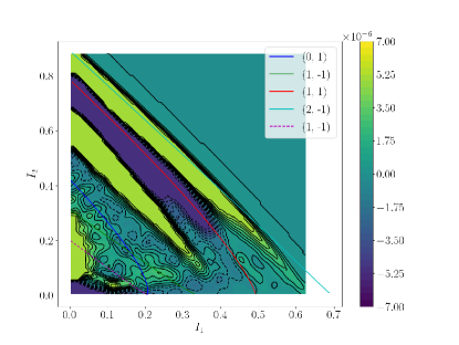
Figure 10: The change in the phase-space distribution function as in Fig. 5 but shown near the peak amplitude in the saturated phase, $T\approx 48$. The loci of the unperturbed resonances from Fig. 5 are shown for comparison.

Figure 10 describes the change in the distribution function from exponential growth at $T=36$ to saturation at $T=48$ (cf. Fig. 5). The change in the phase-space distribution function is characterised by a flat-bottomed valley surrounded by two flat-topped ridges in roughly the same location as the $(l_{1},l_{2})=(1,-1)$ feature in Figure 5. The change in $I_{1},I_{2}$ in the lower left-hand corner of Figure 10 corresponding to $I_{1}\lesssim 0.05,I_{2}\lesssim 0.3$ is caused by the motion of the inner profile as described in Figure 9. These ridge and trough features in the DF suggest that the resonant couple has also saturated. Future work will be necessary to demonstrate whether the origin of the saturation is the radial-angle bunching which detunes the resonance, the secular modification of the bump in the phase-space distribution function, or the interaction of both.

4.3 Combined disc and halo models

This $l=1$ mode will be modified by the gravitational field of the combined disc and halo. Although difficult with the Hamiltonian perturbation theory used in Section 6, a numerical investigation is straightforward with the BFE+mSSA approach. Preliminary results for the evolution of a disc and halo indicates that the $l=1$ halo feature has the same scale and magnitude as described earlier. However, the oblate potential induced by the disc component causes the $l=1$ pattern to nod in the disc plane on an approximately Gyr time scale. This will affect the luminous stellar disc inevitably. This mode could be a natural source of lop-sided asymmetries in Nature and will be the subject of future research.

5 Verification of the instability

We anticipate that some readers will be concerned that the exponentially growth is an artefact of using a BFE method rather than a direct- or tree-gravity code. For example, the BFE technique requires an expansion centre, and this centre may bias the force in such a way to produce a false instability, perhaps? We tested this in two ways:

1. exp can centre the expansion on the minimum of the gravitational potential by ranking the particles by gravitational potential and computing the centre of mass of the 1000 most bound particles. This option is designed for live satellite simulations; the default simulation does not use this option. To test the effect of centring, we resimulated the fiducial run with and without this centring option.

2. We used gadget-2 on the same particle distribution with softening length designed to minimise the force error as described in Dehnen (2001). We used a kd-tree neighbourhood search and kernel density estimation to estimate the local density at each particle position and chose the expansion centre to be the centre of mass for the 1000 highest density particles positions. We then used exp to compute the expansion coefficients from the gadget-2 snapshot files. The same centring scheme was used for both exp and gadget-2 phase-space output for direct comparison.

The results of Test (i) are simple: the results were nearly the same. This further implies that the number of radial basis functions are sufficient to reproduce the density centre displacement in these exp simulation. See Appendix A.3 for additional discussion of centring.

The results of Test (ii) require additional computation to make a fair comparison. The resulting power estimates will be different from the ones in Figure 3 because the density centre is not fixed in inertial space but moving under the influence of the mode and noise. In addition, the centres for the two simulations are now different owing to systematics in the numerical Poisson solvers, although one expects the peak density and minimum potential to be correlated. Nonetheless, the comparison between the $l=1,2$ power computed from the exp and gadget-2 simulations using the kd-tree centring scheme for each (Fig. 11) demonstrates reasonable qualitative and quantitative agreement. Specifically, the $l=1$ shows the same exponential growth rate and the modulation has the same period as the fiducial exp run. Also, the aliased $l=2$ power approximately coincides suggesting that this power is a centring artefact itself. A detailed examination of the centre location reveals that the mean offsets are approximately 0.002 virial units (or 600 pc in Milky Way units) which is very small compared to the average scale of the mode which is 0.05 (or 15 kpc in Milky Way units). It seems safe to conclude that the unstable mode is not an artefact of our BFE-based Poisson solver.

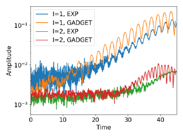
Figure 11: Gravitational amplitude for harmonic orders $l=1,2$ from the gadget-2 and exp simulations and using the same particle distribution from Fig. 3. The expansion centre for each is computed by density estimation from kd-tree neighbourhood search.

6 Insights from linear-response theory

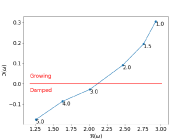
Figure 12: The location of zeros the $\Re(\omega)$–$\Im(\omega)$ plane for the fiducial model with an isotropic distribution function $f(E)$ as a function of truncation index $n$ which defines the width of the truncation function $\sigma_{t}=n/10$ (see Sec. 3).

This section applies linear response theory used in Weinberg (1994) and described in Kalnajs (1977); Fridman & Polyachenko (1984a); Binney & Tremaine (2008) to corroborate the N-body and numerical analyses of the previous sections. In short, we seek the simultaneous solutions of the collisionless Boltzmann and Poisson equations. By representing the density and potential fields by the BFE previously described, this method discretises function space, reducing the solution for modes to the zeros of a determinant, called the dispersion relation. Because this discretisation results in finite-dimension approximation by a matrix, it is often called the matrix method. The linear response code uses the same algorithms as in Weinberg (1989, 1994) although the code has been updated to modern C++-17. Solutions with $\Im(\omega)>0$ ($\Im(\omega)<0$) are growing (decaying). The derivation and evaluation is described in Appendix B. As a basic check, we verified that there are no growing modes for $f=f(E)$ in the untruncated NFW model as demanded by the Antonov theorems. Also, we checked the results quoted for the $l=2$ instabilities in Weinberg (1989) were recovered.

The goal of this section is not to further elucidate the simulations previously described but to demonstrate that the bump on tail instability identified in Section 3 is not dependent on the specifics of our fiducial model (Sec. 2.4). We explore two strategies for modifying the DF to cause a bump. Section 6.1 describes the response frequencies for isotropic distribution function with varying degrees of truncation width, $\sigma_{t}$ (eq. 2). Section 6.3 explores varying anisotropy radii, $r_{q}$, for truncation at 2.5 virial radii. In both cases, the result of truncation and increasing anisotropy is an inflection in the run of $df(E)/dE$ for the isotropic DF and $df(Q)/dQ$ for the Osipkov-Merritt DF. The resonant couples that drive instability depend on the phase-space and model structure in detail and we do not have an explicit criteria for the $l=1$ stability other than the numerical evaluation of the dispersion relation itself. Nonetheless, the examples here suggest that the bump in the DF is the cause.

6.1 Isotropic NFW-like models with varying truncation

We apply the linear response theory to the isotropic distribution functions resulting from Eddington inversion of equation (1) for varying truncation width $\sigma_{t}$. We choose widths $\sigma_{t}=n/10$ for $n=1,\ldots,7$ and the truncation radii $r_{t}=1+3\sigma_{t}$ as described in Section 3 to ensure that the model remains close to the NFW profile at the virial radius and rolls over only at larger radii. The location of the dominant response mode frequencies for $l=1$ is illustrated in Figure 12. The models are $l=1$ unstable for small values of $\sigma_{t}$. By increasing the width of the truncation, the mode crosses the real axis into stability. See Figure 4 for a graphical depiction of these profiles.

The fiducial simulation described in Sections 3 and 4 has $n=2$. For reference, the index $n=2$ corresponds to a truncation width of 1/5 virial radius and truncation radius at 1.6 virial radii. The index $n=5$ corresponds to a truncation width of 1/2 virial radius and truncation radius at 2.5 virial radii. Figure 12 corroborates results of previous sections: the fiducial model is $l=1$ unstable.

This instability appears to result from a bump in the tail of the distribution with $df(E)/dE>0$. The evidence is as follows. The pattern speed, $\Re(\omega)$, of the weakly growing mode is $\sim 1.9$ for the values of $n$ considered (see Fig. 12). As described in Section 3, this frequency decreases to $\sim 1.6$ as the mode grows in amplitude. The pattern frequency matches the orbital frequencies at the same energy as the bump in the DF induced by the truncation (see Fig. 4), suggesting the involvement of a low-order resonance.

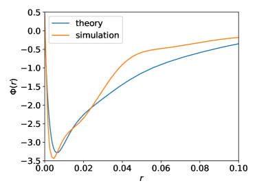
Figure 13: The first PC pair from the mSSA analysis from Sec. 3 at $T=10$ provides the radial profile of the $l=1$ dipole distortion (denoted as simulation). This is compared with the shape of the unstable mode inferred from the linear response analysis (denoted as theory). The overall scaling in amplitude is arbitrary but the shape and position fully determined by the simulation and linear theory.

The linear analysis predicts the eigenfunction (see Appendix B.6) once the frequency is identified. The shape and extent are consistent with the profile inferred from the simulation (Fig 2) and the two are quantitatively compared in Figure 13. This provides further corroboration that the identification of the mode from linear theory is correct. Although we do not expect the linear theory to represent the profile at late times, after non-linear saturation, the qualitative features remain similar.

6.2 Isotropic NFW-like models with varying outer slope

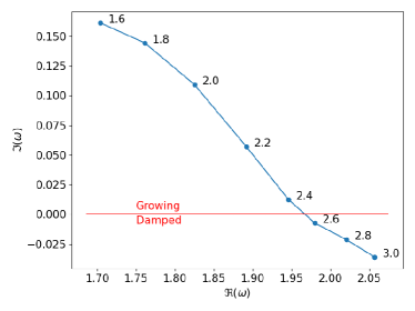
Figure 14: The location of zeros on the $\Re(\omega)$–$\Im(\omega)$ plane for the fiducial model as a function of the outer power-law index $\beta$ (labeled) with the same truncation as the fiducial model. The density $\rho(r)\propto r^{-1-\beta}$ at large $r$. The $\beta=2$ model is the NFW profile and the $\beta=3$ model is the Hernquist profile.

We set the truncation parameter defined in Section 6.1 to $n=2$ and vary the outer slope $\beta$ in equation 1 with $\beta\in[1.6,2.8]$. We fix the inner power-law index to $\alpha=1$, and therefore the density profile for $r>r_{a}$ has $\rho(r)\propto r^{-1-\beta}$. The zeros of the dispersion relation for this sequence is shown in Figure 14. As the density profile steepens, the $l=1$ mode becomes damped. The transition between growing and damped for this truncation occurs at $\beta\approx 2.5$, between the NFW and Hernquist profiles. While researchers often prefer to work with the $\beta=3$ Hernquist model because it has finite mass, the frequency distribution of orbits will be different between $\beta=2$ and $\beta=3$ and this will affect the dynamical response. In this example, the NFW-like model is unstable and the Hernquist-like model is stable. This difference is likely to also affect other astronomically relevant responses, such as satellite wakes. We urge researchers to consider their choice of halo profile carefully and investigate the effect of the outer halo profile.

6.3 Anisotropic NFW-like models

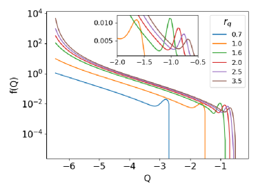
Figure 15: Anisotropic distribution function shown as a function of generalised energy, $Q=E+L^{2}/2r_{q}^{2}$, for various values of anisotropy radius $r_{q}$. We show a value of $r_{q}$ approaching the limiting value for reference; this extreme model is not investigated in this study.

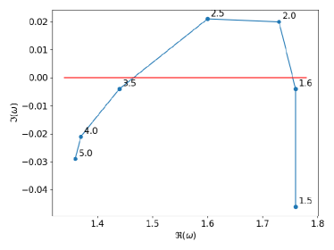
Figure 16: The location of zeros on the $\Re(\omega)$–$\Im(\omega)$ plane for the fiducial model as a function of Osipkov-Merritt anisotropy radius $r_{q}$. Models with a small range of values, $1.6\lesssim r_{q}\lesssim 3.4$, are unstable. In all of these models, the outer halo is modestly anisotropic beyond virial radius and remains isotropic at smaller radii. More importantly, the orbital frequency at location of the induced inflection corresponds to the frequency of the primary mode.

We examine the influence of anisotropy using the Osipkov-Merritt generalisation of the Eddington inversion method for the same density model as in the previous section with $n=5$. While these distribution functions are not good descriptions of DM distributions in cosmological simulations, this distribution function provides a single parameter: the anisotropy radius, $r_{q}$. Section 6.1 shows that the model is stable in isotropic limit, $r_{q}=\infty$. Although one can bias the anisotropy towards both radial and tangential, the radially anisotropic branch yields larger changes in the DF and we restrict our attention to radial anisotropy. The Osipkov-Merritt distribution function has a minimum value of $r_{q}$. For smaller values than this critical value, the distribution function becomes unphysically negative at small energies (i.e. most bound orbits). The critical value for this truncated NFW-like model is $r_{q}\approx 0.5$. The run of DF for a variety of $r_{q}$ values are illustrated in Figure 15. As $r_{q}$ decreases, the high $Q=E+L^{2}/2r_{q}^{2}$ phase space is truncated. This implies that the higher angular momentum orbits are suppressed at high energy; in other words, particles at large radii are eccentric and have much smaller guiding centre radii. This suppresses the lowest frequency orbits.

The zeros of the dispersion relation in the complex $\omega$ plane for $l=1$ are shown in Figure 16. We find that $l=1$ modes are unstable for $1.6\lesssim r_{q}\lesssim 3.4$. This is precisely the energy regime where the bump in $f(Q)$ from Figure 15 overlaps with orbital frequencies at similar values to the pattern speed of the mode, $\Re(\omega)$. For smaller values of $r_{q}$, the frequencies of orbits corresponding to energies in the bump are higher than the natural frequency of the mode, and the mode damps. As $r_{q}$ increases, $\Re(\omega)$ increases and $\Im(\omega)$ decreases; the value approaches that in Figure 12. This anisotropy radius needed for growth is large in model units, two virial radii, suggesting that a very minor amount anisotropy producing a modest bump in $f(Q)$ is sufficient for $l=1$ instability.

As the radial anisotropy approaches approximately 1.5, a different unstable $l=1$ modal track appears along with the $l=2$ ROI. However, the main goal of this investigation is not the dynamical role of anisotropy per se, but a demonstration that the bump in the DF drives the instability. So we will not explore this alternate $l=1$ track here.

We then simulated this same phase-space distribution with $r_{q}=2.0$. This is predicted to be unstable by Figure 16. The modal power for the EXP simulation with $N=1\times 10^{7}$ particles and the same distribution function is shown in Figure 17. The growth for the most unstable value of $r_{q}$ is smaller than for the truncated models (cf. Figures 12 and 16). Nonetheless, the predicted initial growth rates of the two modes are with 30% of the measured values, suggesting that the linear theory captures the essential dynamics at early times. Similar to the initially isotropic case, the pattern speed of the eventual saturated $l=1$ is slower than for the linear mode. The mSSA analysis of the simulation demonstrates that the growing mode has the same character and behaviour as the $l=1$ instability in previous sections.

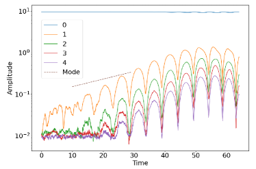
Figure 17: Growth in power for the NFW model with an Osipkov-Merritt radius $r_{q}=2.0$, as described in Figure 3 for the fiducial model. The growth rate predicted by the linear theory (dashed line labeled Mode) is approximately 30% smaller than in the simulation. Qualitatively, the evolution unchanged from the truncated, isotropic fiducial model.

6.4 Single power-law models

The failure to find an $l=1$ unstable King model with an isotropic distribution function (consistent with Weinberg 1991) motivated the consideration of single power-law models with tidal truncations of equation (3) form with $\beta=0$. The mode diagram showing the zeros of the dispersion relation as a function of the power-law exponent $\alpha$ is shown in Figure 18. Power-law exponents $\alpha\lesssim 2.5$ are $l=1$ unstable and and vice versa. This suggests that an extreme core-collapsed globular cluster could be susceptible.

For example, a classical core-collapsed power-law profile of $\alpha\approx 2.3$ (e.g. Baumgardt et al., 2003) would have a growth time of $\sim 0.04$ in virial units. A 100 pc globular cluster with $10^{5}{\rm\,M_{\odot}}$ has a virial time of about 50 Myr, suggesting an $l=1$ growth time of 1 Gyr. In the simulations here, the mode tends to saturate at roughly 10% amplitude; this would produce slight lopsided asymmetry as a function of isophotal radius. There is a preferred axis, so observational detectablity depends on line-of-sight orientation. In addition, the ensemble of eccentric orbits produced by the saturated mode may have implications for the evolution of collisional systems. For example, this population might enhance core-halo momentum transfer and influence predictions made under the assumption of spherically symmetric loss cones.

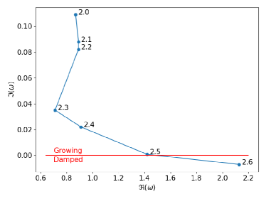
Figure 18: The location of zeros the $\Re(\omega)$–$\Im(\omega)$ plane for a one-power model based on eq. (1) with $\alpha$ indicated and $\beta=0$ and an isotropic distribution function $f(E)$ with truncation width 0.1 in virial units.

7 Discussion and summary

We explored the response of a collisionless halo to an $l=1$ (dipole) distortion using two complementary techniques. First, we performed N-body simulations and quantified the spatial behaviour using a basis-function expansion (BFE). We then used multivariate singular spectrum analysis (mSSA) to identify the correlated temporal changes in the spatial structure encoded by the BFE. For the N-body simulation, the initial distortions are imposed by Poisson fluctuations. Secondly, we used the linear response operator derived for the same BFE to understand the resulting response modes. These modes are not the stationary modes, or by analogy with the plasma literature, the van Kampen (1955) modes of the system, but rather the phase-space structures that result from the linear solution to an initial value problem. For the linear theory, the distortion is any function than can be represented by the expansion. Therefore, the basis must be chosen carefully. The restriction to a finite set of basis functions smooths the distribution to a chosen scale. Conversely, a basis that over smooths important spatial scales will lack sensitivity to small-scale modes. For the $l=1$ mode studied here, the mode is spatially large and easily represented by a truncated basis function expansion.

As described in Section 1, the response modes are of particular interest because they sustain themselves by self gravity and can affect or dress the response of our system at any imposed nearby real frequency. For stable systems, the frequency of these modes have a negative imaginary parts (damped). Most work on stellar spheres considered stability, the most well-known results being Antonov’s stability criteria. However, Weinberg (1994) showed that the $l=1$ modes are often weakly damped albeit stable. Therefore, these may be excited and entrained by minor mergers in a typical galaxian environment and noise in a quiescent environment. Indeed, we have noticed in prior work that the $l=1$ power in the halo component is enhanced relative to $l\geq 2$ in exp simulations and attributed this to dressed noise as described in Weinberg (1994) and more recently by Hamilton & Heinemann (2020). Tracking down the details of this apparently excess power led to the identification of the instability described in this paper.

The key results of this study are as follows:

1. The typically used idealised dark-halo models such as the NFW profile (Navarro, Frenk & White, 1997) are Antonov stable. However, a minor modification that introduces another characteristic scale is enough to promote an $l=1$ instability. For an isotropic distribution function, a truncation between one and two virial radii will promote the instability. The truncation induces an inflection in the phase space distribution function (i.e. some range of $E$ such that $df/dE>0$) that powers the instability.

2. A similarly truncated Hernquist (1990) model remains $l=1$ stable. A thorough investigation of outer power-law slopes of the NFW-like two-power family reveals that the onset of instability occurs for $\beta\lesssim 2.5$ in equation (3). This critical model is in between the outer power-law profiles of the NFW and Hernquist profiles. This leads to a more general implication: the overall shape of the halo profile affects the long-term evolution of galaxies.

3. Single power-law halo profiles, also truncated at between one and two virial radii are unstable for $r^{-\alpha}$ with $\alpha\lesssim 2.5$. This may have implication for star clusters.

4. Truncation per se is not the important feature that determines growth. Rather, a density band or ripple in the outer halo induces an inflection or bump in the phase space distribution function that can power the $l=1$ growth. We demonstrated this using Osipkov-Merritt distributions functions which are also unstable for modest values of anisotropy radius. Their distribution functions have a similar bump or inflection at high energies for finite anisotropy radius.

5. The exponentially growing mode transfers energy and angular momentum from the inner halo to the outer halo. The affected orbits become more eccentric and bunched in radial angle as the mode grows. For our $c=10$ NFW-like model, the peak $l=1$ disturbance occurs at approximately 4 disc scale lengths. Therefore, this mode is likely to influence the disc.

6. Section 3 demonstrates that full realisation of a saturated $l=1$ instability in a DM halo will require more time than the age of current Universe, $t_{0}$. However, scaled to the Milky Way, $t_{o}$ corresponds to $T=7$ in Figures 3 and 17, and the amplitude is already significant. The $l=1$ mode in the DM halo is likely to affect the disc in the current epoch, even before the end of the exponential growth phase. Moreover, the continued accretion of DM through cosmic time produces structure in the outer halo that may enhance coupling and promote instability.

7. The $l=1$ mode is likely to be important in other systems with shorter time scales such as nuclear star clusters (without SMBHs) and possibly globular clusters. The saturated mode presents as a comoving, in phase, overdensity of orbits which may have consequence for collision rates and momentum exchange.

Data availability

The data underlying this article will be shared on reasonable request to the author.

Appendix A The EXP implementation of the biorthogonal expansion

exp allows for a straightforward calculation of the gravitational potential from the mass distribution through time. The key limitation of the BFE method lies in the loss of flexibility owing to the truncation of the expansion: large deviations from the equilibrium disc or halo will not be well represented. Although the basis is formally complete, a truncated expansion limits the variations that can be accurately reconstructed. Despite this, basis functions can be a powerful tool for physical insight; analogous to traditional Fourier analysis, a BFE identifies spatial scales and locations responsible for dynamical evolution. In particular, this paper investigates relatively low-amplitude, large-scale distortions that are well represented by the expansion. Our spherical expansions truncate the series by spherical harmonic order, $l_{max}$, and radial order $n_{max}$.

exp optimally represents the BFE for haloes with radial basis functions determined by the target density profile and spherical harmonics. The lowest-order $l=0,m=0$ basis function matches the potential and density of the equilibrium. Each successive basis function at each harmonic order $l$ introduces variation at a successively smaller spatial scale. Therefore, truncation of this basis function series limits the spatial sensitivity to some minimum spatial scale. For an N-body simulation, this truncation effectively removes the small-scale $1/N$ fluctuations. Therefore, the BFE method would not be an appropriate technique for studying the details of two-body relaxation. Conversely, this is an advantage for approximating a collisionless system.

A.1 Method summary

Any disturbance in an approximately spherical system may be represented as a spherical harmonic expansion with an appropriate set of orthogonal radial wave functions. We choose the biorthogonal potential-density pairs described in Petersen, Weinberg & Katz (2021b). The pair of functions $(u^{lm}_{i},d^{lm}_{i})$ is constructed to satisfy Poisson’s equation, $\nabla^{2}u^{lm}_{i}=4\pi Gd^{lm}_{i}$, and to form a complete set of functions with the scalar the product

$$-\frac{1}{4\pi G}\int dr\,r^{2}u^{lm\,\ast}_{i}(r)d^{lm}_{j}(r)=\begin{cases}1&\mbox{if}\ i=j\\ 0&\mbox{otherwise.}\end{cases}$$ (4)

The total density and potential then have the following expansions:

$$\tilde{\Phi}(\mathbf{r}) = \sum_{lm}Y_{lm}(\theta,\phi)\sum_{j}a^{lm}_{j}(t)u^{lm}_{j}(r),$$ (5)

$$\tilde{\rho}(\mathbf{r}) = \sum_{lm}Y_{lm}(\theta,\phi)\sum_{j}a^{lm}_{j}(t)d^{lm}_{j}(r).$$ (6)

The gravitational potential energy in these fields are:

$$W=\frac{1}{2}\int d^{3}r\tilde{\rho}(\mathbf{r})\tilde{\Phi}(\mathbf{r})=-\frac{1}{2}\sum_{lmj}|a^{lm}_{j}|^{2},$$ (7)

having used the orthogonality properties of the spherical harmonics and biorthogonal functions. The partial sums of the squared coefficients of the expansion are then twice the gravitational potential energy in each harmonic order $l$.

When applied to an N-body simulation, we obtain time series $\mathbf{a}^{lm}_{j}$ for each coefficient in sums in equations (5) and (6). See Petersen, Weinberg & Katz (2021b) for an in-depth discussion of N-body simulation with this gravitational field estimator.

A.2 Parameter choices

The overall fields of the halo are described by $\left(l_{\rm halo}+1\right)^{2}\times n_{\rm halo}$ terms, where $l_{\rm halo}$ is the maximum order of spherical harmonics and $n_{\rm halo}$ is the maximum order of radial terms per $l$ order. For simulations and analyses in this paper, we use a maximum harmonic order $l_{\mbox{\tiny max}}=6$ and maximum radial order $n_{\mbox{\tiny max}}=20$ using the Sturm-Liouville basis conditioned on each particular input model. While the quality of the expansion is centre dependent, the basis could follow any displacement from the centre for sufficiently large particle number and large values of $l_{\mbox{\tiny max}}$ and $n_{\mbox{\tiny max}}$. The choices of $l_{\mbox{\tiny max}}=6$ and $n_{\mbox{\tiny max}}=20$ allows us to follow centre displacements seen in our simulations (see Secs. A.3 and 5 for more discussion). These series of coefficients efficiently describe time dependence of the gravitational field produced by the N-body evolution.

A.3 Centring and momentum conservation

BFE codes such as exp require a choice for the expansion centre. exp monitors the centre of potential by sorting the particles in gravitational energy and computing the centre-of-mass location from the ball enclosing the most bound particles. We have verified that the expansion can reproduce centre shifts of our simulations by showing that two simulations that use the original centre and the centre determined by the most bound particles reproduce the same overall evolution.

Moreover, our research topic is $l=1$ modes in an empty environment. Therefore, dynamical consistency demands that the linear momentum of the entire system be conserved in the presence of a $l=1$ mode. Indeed, this conservation is nearly reproduced by exp; the computed centre of mass for these simulations remains on the initial centre to approximately 0.001 virial radii. The BFE approach does not explicitly conserve momentum by construction, so this is a strong consistency check. Nonetheless, to put to rest concerns that results are affected by centring artefacts, we repeated our fiducial simulation using a tree-gravity Poisson solver which is centre independent by construction; see Section 5.

Appendix B The biorthogonal dispersion relation

B.1 The response matrix

We follow the procedure described in Weinberg (1994) to reduce the coupled system of the collisionless Boltzmann and Poisson equations to a solution of a matrix equation using the expansion above. The solution may then be written as the non-trivial solution to the following linear equation

$${\hat{a}}^{lm}_{i}=M_{ij}(\omega){\hat{a}}^{lm}_{j},$$ (8)

where summations over like indices are implied, the ‘$\hat{\ }$’ indicates a Laplace-transformed quantity, $\omega$ is a complex-valued frequency and

$$M_{ij}(\omega) = \frac{(2\pi)^{3}}{4\pi G}\int\int\frac{dE\,dJ\,J}{\Omega_{1}(E,J)}\sum_{{\bf n}}\frac{2}{2l+1}\times$$ (9)

$${\bf n}\cdot\frac{\partial f_{0}}{\partial{\bf I}}\frac{1}{\omega-{\bf n}\cdot{\bf\Omega}}\left|Y_{l,l_{2}}(\pi/2,0)\right|^{2}\times$$

$$W^{l_{1},\,i\ \ast}_{l,l_{2},l_{3}}({\bf I})W^{l_{1},\,j}_{l,l_{2},l_{3}}({\bf I}),$$

where

$$W^{l_{1}}_{l\,l_{2}l_{3}}(I_{1},I_{2})=\frac{1}{\pi}\int^{\pi}_{0}dw_{1}\cos[l_{1}w_{1}-l_{2}(\psi-w_{2})]u_{j}^{l\,l_{3}}(r).$$ (10)

In the above equations, $I_{1},I_{2},I_{3}$ are the actions, $w_{1},w_{2},w_{3}$ are the angles corresponding to the radial, tangential, and azimuthal action-angle variables and ${\bf n}=(l_{1},l_{2},l_{3})$ is a vector of integers. The actions were chosen by solution of the Hamiltonian-Jacobi equation; $I_{1}$ is the radial action, $I_{2}$ is the total angular momentum and $I_{3}$ is the z-projection of the angular momentum. The quantity $\psi-w_{2}$, the difference between the position angle of a star in its orbital plane and its mean azimuthal angle, depends only on $w_{1}$, the angle describing the radial phase. The frequencies associated with the conjugate angles ${\bf w}$ are defined by ${\bf\Omega}=\partial H/\partial{\bf I}$. The quantity $\Omega_{1}$ is the radial frequency and reduces to the usual epicyclic frequency for nearly circular orbits. The quantity $\Omega_{2}$ is the mean tangential frequency and reduces to the circular orbit frequency, $v_{c}(r)/r$, for orbits with circular velocity $v_{c}$. The quantity $\Omega_{3}=0$ and the corresponding angle $w_{3}$ is the azimuth of the ascending node (see Tremaine and Weinberg 1984, for details). It follows that $M_{ij}^{\ast}(\omega)=M_{ij}(-\omega^{\ast})$ and this property is exploited in the computations described in §3 to reduce the number of numerical evaluations. Since most researchers quote phase-space distribution functions in energy and total angular momentum $f(E,J)$, We have transformed the integration in the definition of ${\bf M}(\omega)$ in equation (9) to $E$ and $J$.

B.2 The dispersion relation

Equation (8) only has a nontrivial solution if

$${\cal D}(\omega)\equiv\hbox{det}\{{\bf 1}-{\bf M}(\omega)\}=0.$$ (11)

As in plasma theory, we refer to the function ${\cal D}(\omega)$ as a dispersion relation. In general, the value of $\omega$ solving equation (11) will be complex. The coefficients $\hat{a}_{j}$ which appear in equation (8) are Laplace transformed and describe the response of the system to a perturbation with a time-dependence of the form $\exp(-i\omega t)$. Because equation (8) follows from a Laplace transform, it is only valid in its present form for $\omega$ in the upper–half complex plane. The dispersion relation must be analytically continued to $\Im(\omega)<0$ to find damped modes. The response coefficients $\hat{\bf a}^{lm}$ which solve equation (8) for a particular eigenfrequency $\omega$, describes a response mode of the system.

Because a sphere has no unique symmetry axis, a response mode can not depend on an arbitrary choice of coordinate axes. Since a rotation causes the azimuthal components indexed by $m$ to mix according to the rotation matrices, the mode itself must depend on $l$ alone. In particular, the functions $(u^{lm}_{i},d^{lm}_{i})$ may be chosen independent of $m$ (e.g. the spherical Bessel function used by Fridman and Polyachenko 1984, and Weinberg 1989). Therefore, equation (9) and the dispersion relation are independent of $m$.

B.3 Convergence

The dispersion relation depends on the response matrix (eq. 9). The elements of this matrix require a two-dimensional quadrature in actions and the computation of the action-angle transform of the biorthogonal potential functions (eq. 10).

The integral in equation (10) defining the angle-action transform is a periodic and therefore has a converging trigonometric expansion owing to the smoothness of the finite-order biorthogonal functions. The Euler-Maclaurin summation formula guarantees that evaluation of a periodic integrand on a uniform grid with $k$ knots will have a negligible error term for sufficiently large $k$. Since $n_{max}=20$, there are at most 20 oscillations in the biorthogonal potential functions. Empirically, a choice of $k=200$ is more than sufficient to compute the $W^{l_{1}}_{l\,l_{2}l_{3}}(I_{1},I_{2})$ to 1 part in $10^{5}$. With these choices, the error in evaluating equation (10) is much smaller than the error in the double quadrature in equation (9).

Turning to the integral in equation (9), the resonant denominator in the integrand is the main source of numerical difficulty. Rather than use the actions $I_{1},I_{2}$ as quadrature variables, we transformed from $I_{1},I_{2}$ to energy and scaled angular momentum variables $E,\kappa$ where $\kappa\equiv I_{2}/J_{max}(E)$ and $J_{max}(E)$ is the angular momentum of the circular orbit with energy $E$. This change was motivated by the behaviour of the ${\bf n}\cdot{\bf\Omega}\approx\mbox{constant}$ loci in each coordinate system. The loci are anti-diagonal in actions $(I_{1},I_{2})$ but tend to lie along lines of constant $\kappa$ in the new variables. Therefore, the choice of $(E,\kappa)$ reduces the total number of necessary quadrature knots. We choose $2^{(n_{E})}$ and $2^{(n_{\kappa})}$ knots in $E$ and $\kappa$, respectively.

The matrix elements in equation (9) also depend on a sum over the integers ${\bf n}$. For the $l=1$ harmonic considered here, $l_{1}\in(-\infty,\ldots,\infty)$, $l_{2}\in[-1,1]$, and $l_{3}\in[-1,1]$. We truncate the sum in $l_{1}$ with the choice $l_{1}\in[-l_{1,max},l_{1,max}]$. In practice, the sum converges quickly in $l_{1,max}$ for two reasons: (1) only a small combination of ${\bf n}$ lead to resonant denominators; and (2) the potential transform (eq. 10) is a Fourier integral which decreases exponentially as $|l_{1}|\rightarrow\infty$.

We demonstrate convergence by exploring the approach to the zero of the dispersion relation (eq. 11) for the unstable $l=1$ mode described in Section 3. The complex frequency of this mode is $\omega_{0}\approx(1.83,0.11)$. First, we choose a set of fiducial values for the parameters which empirically $n_{E}=7,n_{\kappa}=5,l_{1,max}=8$ which are close to converged. We evaluate sequences of $\omega$ with ${\cal D}(\omega)=0$ by increasing each of $n_{E},n_{\kappa},l_{1,max}$ in turn while the others remain at their fiducial value. Figure 19 shows the modulus of the difference between these parameters and the last one in the sequence. The relative error in $\omega_{0}$ decreases as each of $n_{E},n_{\kappa},l_{1,max}$ increase. As expected, the dependence on $n_{\kappa}$ is weak while the convergence in $n_{E}$ is slower, approaching a relative error of approximately $5\times 10^{-4}$ af the end of the sequence. The larger values of $l_{1}$ do affect the location of $\omega_{0}$ but $l_{1,max}=8$ does seem sufficient for the purposes of this work.

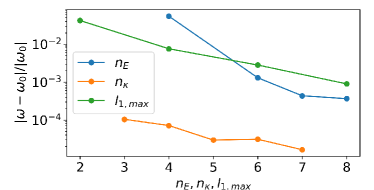
Figure 19: The relative difference for the zero of the dispersion, as each of the parameters $n_{E},n_{\kappa},l_{1,max}$ are increased in turn. Each solution, $\omega$, is compared to the solution for the largest parameter value in the sequence, $\omega_{0}$. The complex frequency of this mode is $\omega_{0}\approx(1.83,0.11)$. The two non-varying parameters in each sequence are set to $n_{E}=7,n_{\kappa}=5,l_{1,max}=8$. The series converge with relative errors in $\omega$ are ${\cal O}(10^{-3})$ for the working parameter set.

B.4 Evaluating the response matrix

B.4.1 Application to cuspy halo

We evaluate a grid of orbital parameters at the positions of the $E,\kappa$ knots used to perform the quadratures for the the matrix elements (eq. 9). At each pair $E,\kappa$, the linear response code computes the actions $I_{1},I_{2}$, the inner and outer turning points, the frequencies $\Omega_{1},\Omega_{2}$ and the run of radius as a function of the radial angle and the difference between the azimuth and mean azimuth, $\psi-w_{2}$. For the $r^{-1}$ cusps considered here (see Sec. 2.4), the orbital frequencies are proportional to $r^{-1/2}$. While there is no fundamental numerical problem computing these values in a cusp, including a core radius in the model results in bounded frequency values and prevents hand-tuning the root finders used to compute orbital turning points. One can accomplish the same result by choosing the lower end point of the energy integral offset very slightly from the potential value at $r=0$.

For the small values of $r_{c}$ used for our fiducial model, the mass fraction inside of $r_{c}$ is approximately $3\times 10^{-7}$ of the total. It is possible that our choice of finite $r_{c}$ could affect the value of ${\cal D}(\omega)$ for values of $\omega\sim\Omega_{1,2}$ at radii inside of $r_{c}$. However, these orbital frequencies are so large compared to our modal frequencies that that resonant coupling is not possible. On the N-body side, we have repeated the simulation with zero core radius and there is no distinguishable difference.

B.4.2 Mode location

The zeros of the dispersion relation, equation (11), that determine the point-mode locations are found in two steps:

1. We begin by evaluating ${\cal D}(\omega)$ over a coarse grid with 20 or 40 real frequencies and 5 or 10 imaginary frequencies. We know a priori that the real frequencies of the weakly damped or weakly growing modes will be in the range $\Re(\omega)=[0,20]$ in units where the gravitational constant, mass and outer radius are unity. We choose $\Im(\omega)=[0,0.2]$. A visual inspection of the $|{\cal D}(\omega)|$ surface will reveal the locations of an unstable mode in the upper-half plane as a zero or a damped mode in the lower-half as a trough decreasing towards $\Im(\omega)\rightarrow 0$.

2. If the mode is in the upper half plane, we attempt to isolate the mode with successively refined $10\times 10$ grids bracketing the zero in $|{\cal D}(\omega)|$. We determine the mode by using bilinear interpolation to find the zero-valued loci in $\Re({\cal D})$, $\Im({\cal D})$ and find the intersection of these two loci to estimate the solution. If the mode is in the lower half plane, we use the rational function extrapolation technique described in Weinberg (1994) to estimate values of ${\cal D}(\omega)$ in the vicinity of the zero. We recommend using 30 or fewer $\omega$ points as input to the rational function construction algorithm. For the results in Section 6, we typically used used a grid of 8 in $\Re({\omega})$ by 3 in $\Im({\omega})$ spaced around the trough in $\Re({\omega})$ and a height in $\Im({\omega})$ of order the scale length in the trough’s gradient. Large numbers of $\omega$ points may result in nearly cancelling roots in the numerator and denominator of the rational function. These lead to numerical artefacts from incomplete cancellation. It should be possible to apply a heuristic to remove these pairs of roots, but that has not been done here.

B.5 The $l=1$ neutral translation mode

In addition to the point modes that we use interpret our simulations described in Section 6, the response matrix admits a zero-frequency $l=1$ mode. This point mode corresponds to a body displacement of the system. Conservation of linear momentum prohibits self excitation of this mode; it can only be excited by external perturbation that applies a net force to the initially unperturbed system. The conservation of linear momentum has been addressed in Appendix A.3.

In addition, the biorthogonal basis derived using solutions of the Sturm-Liouville equation (Weinberg, 1999; Petersen, Weinberg & Katz, 2021b) provides variation in and around the characteristic radius of the system but not at small and large radii. Therefore, the translation mode converges very slowly in the cusp. Fortunately, this mode has no bearing on the analyses in §6.

B.6 Derivation of the point-mode shape and the system response

The modal eigenvector $\hat{a}_{j}$ can be easily found through singular value analysis of the response matrix (eq. 9) evaluated at the modal frequency. The desired eigenvector will have eigenvalue $\lambda\approx 1$. The proximity of $\lambda$ to $1$ provides a self-consistency check on the numerics of the dispersion relation. Typically, these values are $\lambda=1\pm 0.05$. The density and potential perturbations follow directly using equations (5) and (6). For an unstable mode, it is sufficient to determine the eigenvalues and eigenvectors of ${\cal D}(\omega)$ at the modal frequency. For a stable damped mode, the matrix elements can be estimated by the same rational function extrapolation method used in Section B.4.2 (see Weinberg 1994).

References

- Antonov (1962) Antonov V. A., 1962, Vestnik Leningrad Univ., 96, 19
- Antonov (1973) Antonov V. A., 1973, The Dynamics of Galaxies and Star Clusters, Omarov G. B., ed., Reidel, Dordrecht, p. 531, english transl. in Structure and Dynamics of Elliptical Galaxies, ed. T. de Zeeuw
- Baumgardt et al. (2003) Baumgardt H., Heggie D. C., Hut P., Makino J., 2003, MNRAS, 341, 247
- Binney & Tremaine (2008) Binney J., Tremaine S., 2008, Galactic Dynamics: (Second Edition) (Princeton Series in Astrophysics). Princeton University Press
- Clutton-Brock (1972) Clutton-Brock M., 1972, Ap&SS, 16, 101
- Clutton-Brock (1973) Clutton-Brock M., 1973, Ap&SS, 23, 55
- De Rijcke, Fouvry & Pichon (2019) De Rijcke S., Fouvry J.-B., Pichon C., 2019, MNRAS, 484, 3198
- Dehnen (2001) Dehnen W., 2001, MNRAS, 324, 273
- Diemer & Kravtsov (2014) Diemer B., Kravtsov A. V., 2014, ApJ, 789, 1
- Dubois et al. (2021) Dubois Y. et al., 2021, A&A, 651, A109
- Fouvry et al. (2021) Fouvry J.-B., Hamilton C., Rozier S., Pichon C., 2021, MNRAS, 508, 2210
- Fouvry et al. (2015) Fouvry J. B., Pichon C., Magorrian J., Chavanis P. H., 2015, A&A, 584, A129
- Fridman & Polyachenko (1984a) Fridman A. M., Polyachenko, 1984a, Physics of Gravitating Systems II. Springer-Verlag, New York
- Fridman & Polyachenko (1984b) Fridman A. M., Polyachenko V. L., 1984b, Physics of Gravitating Systems, Vol. 2, Springer-Verlag, New York, p. 282
- Ghil & Vautard (1991) Ghil M., Vautard R., 1991, Nature, 350, 324
- Golyandina, Nekrutkin & Zhigljavsky (2001) Golyandina N., Nekrutkin V., Zhigljavsky A. A., 2001, Analysis of time series structure: SSA and related techniques. Chapman and Hall/CRC
- Hamilton & Heinemann (2020) Hamilton C., Heinemann T., 2020, arXiv e-prints, arXiv:2011.14812
- Heggie, Breen & Varri (2020) Heggie D. C., Breen P. G., Varri A. L., 2020, MNRAS, 492, 6019
- Hernquist (1990) Hernquist L., 1990, 356, 359
- Hernquist & Ostriker (1992) Hernquist L., Ostriker J. P., 1992, ApJ, 386, 375
- Ichimaru (1973) Ichimaru S., 1973, Basic Principles of Plasma Physics. W. A. Benjamin, Reading
- Ikeuchi, Nakamura & Takahara (1974) Ikeuchi S., Nakamura T., Takahara F., 1974, Progress of Theoretical Physics, 52, 1807
- Johnson et al. (2023) Johnson A., Petersen M. S., Johnston K., Weinberg M. D., 2023, MNRAS, 521, 1757
- Kalnajs (1977) Kalnajs A. J., 1977, 212, 637
- Landau (1946) Landau L. D., 1946, JETP, 10, 25
- Lau & Binney (2021) Lau J. Y., Binney J., 2021, MNRAS, 507, 2241
- M. Ghil et al. (2002) M. Ghil M. et al., 2002, Rev. Geophys., 40, 1.1
- McMillan (2017) McMillan P. J., 2017, MNRAS, 465, 76
- Merritt (1985) Merritt D., 1985, 90, 1027
- Monachesi et al. (2019) Monachesi A. et al., 2019, MNRAS, 485, 2589
- Navarro, Frenk & White (1997) Navarro J. F., Frenk C. S., White S. D. M., 1997, ApJ, 490, 493
- Nelson et al. (2018) Nelson D. et al., 2018, The illustristng simulations: Public data release
- Osipkov (1979) Osipkov L. P., 1979, sal, 5, 42, pis’ma astron. zh., vol. 5, 77-80 (1979) in Russian
- Palmer (1994) Palmer P. L., 1994, Stability of collisionless stellar systems: mechanisms for the dynamical structure of galaxies, Vol. 185. Kluwer
- Palmer & Papaloizou (1987) Palmer P. L., Papaloizou J., 1987, MNRAS, 224, 1043
- Petersen (2020) Petersen M. S., 2020, private communication
- Petersen, Weinberg & Katz (2019a) Petersen M. S., Weinberg M. D., Katz N., 2019a, arXiv e-prints, arXiv:1902.05081
- Petersen, Weinberg & Katz (2019b) Petersen M. S., Weinberg M. D., Katz N., 2019b, arXiv e-prints, arXiv:1903.08203
- Petersen, Weinberg & Katz (2019c) Petersen M. S., Weinberg M. D., Katz N., 2019c, MNRAS, 490, 3616
- Petersen, Weinberg & Katz (2021a) Petersen M. S., Weinberg M. D., Katz N., 2021a, arXiv e-prints, arXiv:2104.14577
- Petersen, Weinberg & Katz (2021b) Petersen M. S., Weinberg M. D., Katz N., 2021b, arXiv e-prints, arXiv:2104.14577
- Riesz & Nagy (2012) Riesz F., Nagy B., 2012, Functional Analysis, Dover Books on Mathematics. Dover Publications
- Springel (2005) Springel V., 2005, MNRAS, 364, 1105
- Tremaine & Weinberg (1984) Tremaine S., Weinberg M. D., 1984, MNRAS, 209, 729
- van Kampen (1955) van Kampen N. G., 1955, Physica, 21, 949
- Weinberg (1989) Weinberg M. D., 1989, MNRAS, 239, 549
- Weinberg (1991) Weinberg M. D., 1991, ApJ, 368, 66
- Weinberg (1994) Weinberg M. D., 1994, AJ, 108, 1414
- Weinberg (1994) Weinberg M. D., 1994, ApJ, 421, 481
- Weinberg (1999) Weinberg M. D., 1999, AJ, 117, 629
- Weinberg & Petersen (2021) Weinberg M. D., Petersen M. S., 2021, MNRAS, 501, 5408
- Wetzel et al. (2022) Wetzel A. et al., 2022, Public data release of the fire-2 cosmological zoom-in simulations of galaxy formation