A topological proof that there is no sign problem in one dimensional Path Integral Monte Carlo simulation of fermions

Abstract

This work shows that, in one dimension, due to its topology, a closed-loop product of short-time propagators is always positive, despite the fact that each anti-symmetric free fermion propagator can be of either sign.

I Introductions

In their first path-integral Monte Carlo (PIMC) simulation of fermions in a one-dimensional harmonic oscillator, Takahashi and Imada were surprised that, “In the calculation of one-dimensional fermions, we do not find any cases of negative weight function in ten thousands Monte Carlo steps even at low temperature”tak84 . They surmised that their situation maybe similar to the one-dimensional lattice fermions studies of Hirsch, Scalapino, Sugar and Blankenbeckerhir81 . The two are not similar. By a clever lattice arrangement, the matrix elements of Hirsch et al.’s lattice fermions can be chosen to be positivehir81 , while the free fermion propagator used by Takahashi and Imada can have either sign. However, 24 years earlier, Girardeaugir60 has shown that, in one dimension, the ground state wave function of $N$ impenetrable bosons $\{x_{1},x_{2}\cdots x_{n}\}$, which vanishes whenever $x_{i}=x_{j}$, is the same as the modulus of the ground state wave function of $N$ free fermions:

$$\psi_{0}^{B}=|\psi_{0}^{F}|.$$ (1)

This means that, in one dimension, $N$ interacting fermions can always be mapped into the ordered subspace

$$x_{1}<x_{2}<\cdots<x_{N},$$ (2)

with vanishing wave function at $x_{i}=x_{i+1}$. The ground state wave function can then be taken to be positive, the same as that of $N$ impenetrable, interacting bosonsneg88 . Alternatively, one can view the subspace (2) as having the correct wave function nodes at $x_{i}=x_{i+1}$, thereby reduced a many-fermion problem, to that of a many-boson problem in a single nodal regioncep91 . Both views explain that fermions in one dimension do not have the sign problem because it is basically a boson problem.

However, these two views do not explain why there is no sign problem specifically for PIMC simulations, despite the fact that the anti-symmetric free fermion propagator can have either sign and that the simulation is not restricted to any particular nodal region.

This work found that there is a surprisingly simple, but overlooked topological proof, that there is no sign problem for PIMC simulation of one dimensional fermions. This topological explanation is related to the original insight of Girardeaugir65 , that any statistics is permissible in one dimension, but only Fermi-Dirac or Bose-Einstein statistics is mandated in more than one dimension.

II Fermion Path Integral Monte Carlo

Consider the single particle imaginary time Schrödinger equation in one-dimension,

$$-\frac{\partial\psi(x,\tau)}{\partial\tau}=(\hat{T}+\hat{V})\psi(x,\tau)=\left(-\frac{1}{2}\frac{\partial^{2}}{\partial x^{2}}+V(x)\right)\psi(x,\tau),$$ (3)

with dimensionless spatial variable $x$ and imaginary time $\tau$. In PIMC, one is interested in extracting the ground state wave function squared $\psi^{2}_{0}(x)$ and energy $E_{0}$ from the diagonal element of the imaginary time propagator at the large time limit:

$$\lim_{\tau\rightarrow\infty}G(x,x;\tau)\longrightarrow\psi_{0}^{2}(x){\rm e}^{-\tau E_{0}}+\cdots,$$ (4)

where

$$G(x^{\prime},x;\tau)=\langle x^{\prime}|{\rm e}^{-\tau(\hat{T}+\hat{V})}|x\rangle=\sum_{n}\psi_{n}^{*}(x^{\prime})\psi_{n}(x){\rm e}^{-\tau E_{n}}.$$ (5)

Since $G(x^{\prime},x;\tau)$ is generally unknown, it is approximated by $k$ short-time propagators via

$$G_{k}(x^{\prime},x;\tau) = \langle x^{\prime}|({\rm e}^{-{\epsilon}(\hat{T}+\hat{V})})^{k}|x\rangle$$ (6)

$$= \int_{-\infty}^{\infty}dx_{1}\cdots dx_{k-1}\,G_{1}(x^{\prime},x_{1};{\epsilon})G_{1}(x_{1},x_{2};{\epsilon})\cdots G_{1}(x_{k-1},x;{\epsilon}),$$

where ${\epsilon}=\tau/k$ and $G_{1}(x^{\prime},x,{\epsilon})$ is usually the second-order short-time approximation of $\langle x^{\prime}|{\rm e}^{-{\epsilon}(\hat{T}+\hat{V})}|x\rangle$, the primitive approximation (PA) propagator:

$$G_{1}(x^{\prime},x;{\epsilon})=\langle x^{\prime}|{\rm e}^{-({\epsilon}/2)\hat{V}}{\rm e}^{-{\epsilon}\hat{T}}{\rm e}^{-({\epsilon}/2)\hat{V}}|x\rangle$$

$$\qquad=\frac{1}{\sqrt{2\pi{\epsilon}}}{\rm e}^{-({\epsilon}/2)V(x^{\prime})}{\rm e}^{-(x^{\prime}-x)^{2}/(2{\epsilon})}{\rm e}^{-({\epsilon}/2)V(x)}.$$ (7)

To generalize the above to $N$ fermions, one replaces $x$ by ${\bf x}=(x_{1},x_{2}\cdots x_{N})$ and $G_{1}(x^{\prime},x,{\epsilon})$ by

$$G_{1}({\bf x}^{\prime},{\bf x};{\epsilon})={\rm e}^{-({\epsilon}/2)V({\bf x}^{\prime})}G_{0}({\bf x}^{\prime},{\bf x};{\epsilon}){\rm e}^{-({\epsilon}/2)V({\bf x})},$$ (8)

where $G_{0}({\bf x}^{\prime},{\bf x};{\epsilon})$ is the anti-symmetric free-fermion propagator

$$G_{0}({\bf x}^{\prime},{\bf x};{\epsilon}) = \frac{1}{N!}{\rm det}\left(\frac{1}{\sqrt{2\pi{\epsilon}}}\exp\left[-\frac{1}{2{\epsilon}}(x_{i}^{\prime}-x_{j})^{2}\right]\right).$$ (9)

Note that any pair exchange $x^{\prime}_{i}\leftrightarrow x^{\prime}_{j}$ ($x_{i}\leftrightarrow x_{j}$) interchanges two rows (columns) of the determinant and hence the sign of $G_{0}({\bf x}^{\prime},{\bf x};{\epsilon})$, while $G_{0}({\bf x}^{\prime},{\bf x};{\epsilon})=G_{0}({\bf x},{\bf x}^{\prime};{\epsilon})$.

III No sign problem in one dimension

The sign of the integrand in the discrete path integral (6) depends only on the product of $k$ free-fermion propagators:

$$G_{0}({\bf x},{\bf x}_{1};{\epsilon})G_{0}({\bf x}_{1},{\bf x}_{2};{\epsilon})\cdots G_{0}({\bf x}_{k-1},{\bf x};{\epsilon}).$$ (10)

For extracting $\psi_{0}^{2}({\bf x})$, the propagators must start at ${\bf x}$ and loop back to ${\bf x}$. The integral is that of a closed-end path-integral. Consider first, the case of two (spinless) fermions. The anti-symmetric free propagator is then

$$G_{0}(x_{1}^{\prime},x_{2}^{\prime},x_{1},x_{2};{\epsilon}) = \frac{1}{2}\frac{1}{2\pi{\epsilon}}\det\left(\begin{array}[]{cc}{\rm e}^{-\frac{1}{2{\epsilon}}(x^{\prime}_{1}-x_{1})^{2}}&{\rm e}^{-\frac{1}{2{\epsilon}}(x^{\prime}_{1}-x_{2})^{2}}\\ {\rm e}^{-\frac{1}{2{\epsilon}}(x^{\prime}_{2}-x_{1})^{2}}&{\rm e}^{-\frac{1}{2{\epsilon}}(x^{\prime}_{2}-x_{2})^{2}}\end{array}\right)$$ (13)

$$= \frac{1}{2}\frac{1}{2\pi{\epsilon}}{\rm e}^{-\frac{1}{2{\epsilon}}\left[(x_{1}^{\prime}-x_{1})^{2}+(x_{2}^{\prime}-x_{2})^{2}\right]}\left(1-{\rm e}^{-\frac{1}{{\epsilon}}(x_{1}^{\prime}-x^{\prime}_{2})(x_{1}-x_{2})}\right).$$ (14)

Thus $G_{0}(x_{1}^{\prime},x_{2}^{\prime},x_{1},x_{2};{\epsilon})<0$ if and only if

$$(x_{1}^{\prime}-x_{2}^{\prime})(x_{1}-x_{2})<0,$$ (15)

i.e., either $x_{1}^{\prime}>x_{2}^{\prime}$ and $x_{1}<x_{2}$ or vice versa. This means that the prime and unprime positions are on opposite sides of the line $x_{1}=x_{2}$ dividing the $x_{1}-x_{2}$ plane.

The key contribution of this work is to rephrase the above condition in topological terms: the propagator is negative when the line connecting the prime and unprime position of the propagator crosses the line $x_{1}=x_{2}$. This is shown in part A of Fig.1. For two propagators $G_{0}({\bf x},{\bf x}_{1};{\epsilon})G_{0}({\bf x}_{1},{\bf x};{\epsilon})$, the line is either not crossed or crossed twice and the product is always positive. The same is true for the product of three propagators $G_{0}({\bf x},{\bf x}_{1};{\epsilon})G_{0}({\bf x}_{1},{\bf x}_{2};{\epsilon})G({\bf x}_{2},{\bf x};{\epsilon})$, as shown in part B. More generally, any closed-loop product of propagators must be positive, as shown in part C, since topologically, any planar closed curve must intersect an infinite straight line even number of times.

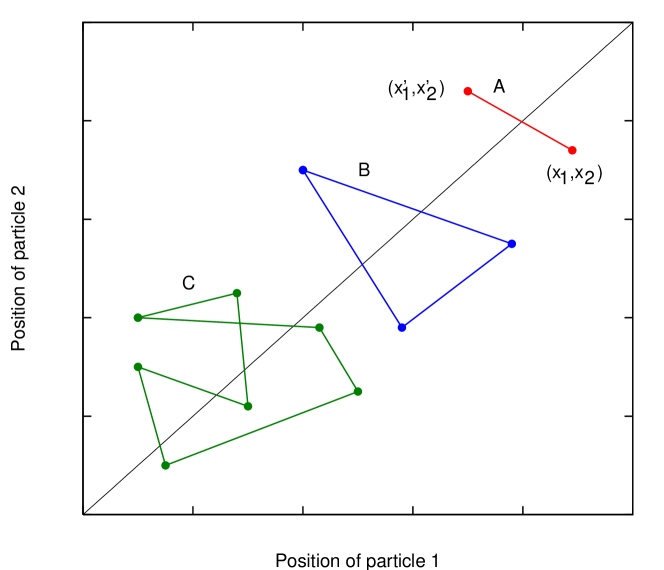
Figure 1: In one dimension, the product of two-particle anti-symmetric propagators in a closed-loop must cross the line $x_{2}=x_{1}$ an even number of times.

For $N$ fermions, the positions of the anti-symmetric propagator are defined in a $N$-dimensional manifold. The propagator changes sign whenever its initial and final position cross any one of the $N(N-1)/2$, ($N-1$)-dimensional hyper-planes defined by $x_{i}=x_{j}$. Since each such ($N-1$)-dimensional hyper-planes completely divides the $N$-dimensional manifold into two halves, any closed curve in the $N$-dimensional manifold must pierce each such hyper-plane even number of times. Thus a closed-loop product of free-fermion propagators for $N$ fermions is also always positive.

IV Sign problem in more than one dimension

In $d$-dimension, one replaces $x_{i}$ by $d$-dimensional vectors ${\bf r}_{i}=(x_{i},y_{i},z_{i},\cdots)$ and set ${\bf x}=({\bf r}_{1},{\bf r}_{2}\cdots{\bf r}_{N})$. In this case the anti-symmetric two-fermion free propagator is

$$G_{0}({\bf r}_{1}^{\prime},{\bf r}_{2}^{\prime},{\bf r}_{1},{\bf r}_{2};{\epsilon}) = \frac{1}{2}\frac{1}{(2\pi{\epsilon})^{d}}{\rm e}^{-\frac{1}{2{\epsilon}}\left[({\bf r}_{1}^{\prime}-{\bf r}_{1})^{2}+({\bf r}_{2}^{\prime}-{\bf r}_{2})^{2}\right]}\left(1-{\rm e}^{-\frac{1}{{\epsilon}}({\bf r}_{1}^{\prime}-{\bf r}^{\prime}_{2})\cdot({\bf r}_{1}-{\bf r}_{2})}\right),$$ (16)

and vanishes whenevercep91

$$({\bf r}_{1}^{\prime}-{\bf r}^{\prime}_{2})\cdot({\bf r}_{1}-{\bf r}_{2})=0.$$ (17)

In two-dimension, the two-fermion propagator is defined in the four-dimensional manifold $(x_{1},y_{1},x_{2},y_{2})$, and vanishes at the coincident planecep91 given by $x_{1}=x_{2}$ and $y_{1}=y_{2}$. This is the direct generalization of the one dimensional case. However, in this case, the coincident plane is only two dimensional, two dimensions less than the full manifold and therefore does not divide the four-dimensional manifold into disjoint regionsgir65 . (This is similar to the case of a line, which is two dimensions less than, and therefore cannot divide, the three dimensional Euclidean space.) (Away from the coincident plane, the propagator, according to (17), can also vanishes if the relative vector ${\bf r}^{\prime}_{12}={\bf r}_{1}^{\prime}-{\bf r}^{\prime}_{2}$ is perpendicular to the relative vector ${\bf r}_{12}={\bf r}_{1}-{\bf r}_{2}$. In two dimension, ${\bf r}_{12}$ can be oriented at an arbitrary angle $\phi$. Thus away from the coincident plane, the propagator can additionally vanishes at two one-dimensional circles. This measure zero effect can be ignored.) Therefore, in the four-dimensional manifold $(x_{1},y_{1},x_{2},y_{2})$, a closed curve can either pierces the coincident plane, or goes around it. Thus a closed-loop product of anti-symmetric propagators can be of either sign and one has a sign problem.

Generalizing this to $N$ particles in $d$-dimension, the propagator is defined in a $Nd$-dimensional manifold. Any coincident plane is of dimension ($Nd-d$) and cannot fully divide the $Nd$-dimensional manifold except for $d=1$. Therefore, the sign problem is generally pervasive except in one dimension.

V Concluding remarks

The observation that a $Nd$-dimensional manifold remains connected, despite the existence of ($Nd-d$) dimensional coincident hyper-planes, was Girardeau’sgir65 insight that the conventional proof for Fermi-Dirac or Bose-Einstein statistics only applies to $d>1$. (The loop-hole for anyon statistics in $d=2$ was a later developmentlei77 ; wil82 .) For $d=1$, since each coincident plane completely divides the manifold, statistics based any permutation symmetry is permissiblegir65 . Here, it provided a simple proof that there is no sign problem in PIMC simulations of fermions in one dimension.

References

• (1) M. Takahashi and M. Imada, J. Phys. Soc. Jpn. 53, 963 (1984).
• (2) J. Hirsch, D. J. Scalapino, R. L. Sugar and and R. Blankenbecker, Phys. Rev. Lett. 47, 1628 (1981); Phys. Rev. B 26, 5033 (1982).
• (3) M. D. Girardeau, J. Math. Phys. 1, 516 (1960)
• (4) J. W. Negele and H. Orland, Quantum Many-Particle Systems, Addison-Wesley, Reading, Massachusetts, 1988.
• (5) D. M. Ceperley, J. Stat. Phys. 63, 1237 (1991).
• (6) M. D. Girardeau, Phys. Rev. 139, 501 (1965).
• (7) J. M. Leinaas and J. Myrheim, Il Nuovo Cimento B 37, 1 (1977)
• (8) F. Wilczek, Phys. Rev. Lett. 49, 957 (1982).