Unravelling the edge spectra of non-Hermitian Chern insulators

Abstract

Non-Hermitian Chern insulators differ from their Hermitian cousins in one key aspect: their edge spectra are incredibly rich and confounding. For example, even in the simple case where the bulk spectrum consists of two bands with Chern number $\pm 1$, the edge spectrum in the slab geometry may have one or two edge states on both edges, or only at one of the edges, depending on the model parameters. This blatant violation of the familiar bulk-edge correspondence casts doubt on whether the bulk Chern number can still be a useful topological invariant, and demands a working theory that can predict and explain the myriad of edge spectra from the bulk Hamiltonian to restore the bulk-edge correspondence. We outline how such a theory can be set up to yield a thorough understanding of the edge phase diagram based on the notion of the generalized Brillouin zone (GBZ) and the asymptotic properties of block Toeplitz matrices. The procedure is illustrated by solving and comparing three non-Hermitian generalizations of the Qi-Wu-Zhang model, a canonical example of two-band Chern insulators. We find that, surprisingly, in many cases the phase boundaries and the number and location of the edge states can be obtained analytically. Our analysis also reveals a non-Hermitian semimetal phase whose energy-momentum spectrum forms a continuous membrane with the edge modes transversing the hole, or genus, of the membrane. Subtleties in defining the Chern number over GBZ, which in general is not a smooth manifold and may have singularities, are demonstrated using examples. The approach presented here can be generalized to more complicated models of non-Hermitian insulators or semimetals in two or three dimensions.

I Introduction

In recent years, substantial progress has been made in characterizing the topological properties of non-Hermitian Hamiltonians describing non-interacting particles hopping on periodic lattices Ashida et al. (2020); Bergholtz et al. (2021); Okuma and Sato (2022); Ghatak and Das (2019). Despite its apparent simplicity, many aspects of the problem, especially in dimensions higher than one, still remain shrouded in mystery and lack the same level of completeness or clarity as the Hermitian topological phases of matter. To motivate our paper and to pinpoint the problem, we jump right to a concrete model. More detailed discussions of the background, including previous results that inspired and influenced our paper, will be given in Sec. VI.

I.1 The Qi-Wu-Zhang model

We are interested in the non-Hermitian generalizations of Chern insulators in two dimensions (2D). A simple example of Hermitian Chern insulators is a two-band model introduced by Qi, et al. on a square lattice Qi et al. (2006). Its Hamiltonian reads

$$H_{0}(\mathbf{k}) = \mathbf{d}(\mathbf{k})\cdot\boldsymbol{\sigma}$$

$$= \sin k_{x}\sigma_{x}+\sin k_{y}\sigma_{y}+(m-\cos k_{x}-\cos k_{y})\sigma_{z},$$

where $\mathbf{k}=(k_{x},k_{y})$ is the crystal momentum, $\boldsymbol{\sigma}=(\sigma_{x},\sigma_{y},\sigma_{z})$ denotes the Pauli matrices to describe the two orbital degrees of freedom (pseudo-spin 1/2), and the momentum-dependent “magnetic field” $\mathbf{d}=(d_{x},d_{y},d_{z})$ with $d_{x}=\sin k_{x}$, $d_{y}=\sin k_{y}$, $d_{z}=m-\cos k_{x}-\cos k_{y}$. The tuning parameter $m$ is real and plays the role of Dirac mass to dictate the energy gap. Note that the energy is always measured in units of the nearest-neighbor hopping $t$ which we have set to be 1. The Qi-Wu-Zhang model Eq. (I.1) has the virtue of being mathematically elegant with a clean-cut phase diagram Qi et al. (2006): For $|m|<2$, the system is topologically nontrivial with the Chern numbers of the two bands being $\pm 1$, the energy gap closes when $m=\pm 2$, and the system becomes topologically trivial for $|m|>2$. From the Chern numbers of the bands, we immediately know that there is one chiral edge mode inside the energy gap for $|m|<2$.

I.2 Three non-Hermitian generalizations

A few different non-Hermitian generalizations of the Qi-Wu-Zhang model have been considered in the literature. Below, we will analyze and compare three examples. They are obtained by adding one extra term to the Qi-Wu-Zhang model $H_{0}$, resulting in increasing complexity in the edge spectra. The first model is

$$H_{1}=H_{0}+ih_{z}\sigma_{z}.$$ (2)

The constant $h_{z}$ term introduces an imaginary part to the “magnetic field” $\mathbf{d}$ by replacing $d_{z}\rightarrow d_{z}+ih_{z}$ while retaining $d_{x,y}$ in $H_{0}$. In Ref. Xu et al. (2017), a three-dimensional generalization (with $k_{z}$) of this model was used to discuss Weyl exceptional rings. This model will be analyzed in Sec. III, and its phase diagram in the slab geometry (e.g., with open boundaries in the $x$ direction, $x\in[0,L]$, and periodic boundary condition along $y$) is summarized in Fig. 1(a). We use $H_{1}$ as a warm-up example to set the stage for models $H_{2}$ and $H_{3}$ below, which feature much more complicated phase diagrams.

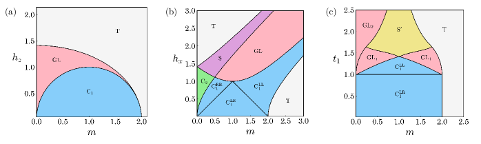
Figure 1: Summary of main results: A myriad of phases of non-Hermitian Chern insulators in slab geometry, $x\in[0,L]$ in the limit of large $L$ with periodic boundary conditions along $y$. The three panels (a)-(c) show the phase diagram for the generalized Qi-Wu-Zhang model $H_{1}$, $H_{2}$, and $H_{3}$, respectively. For model $H_{1}$ in (a), there are three phases indicated by color: the gapped topological phase with Chern number $\pm 1$ (C₁), the gapless phase (GL), and the trivial band insulator (T). This model is discussed in Sec. III. For $H_{2}$ in (b), the C₁ phase is further partitioned into three regions, where the subscripts such as LR describe the localization of the edge modes. There is also a gapped phase C₂ with Chern number $\pm 2$, and a topological gapless phase S. Both are unexpected from the bulk phase diagram. See Sec. IV for details. For model $H_{3}$ in (c), the C₁ phase has two regions with distinct edge behaviors, and a topological gapless phase S^′ (Sec. V).

The second model is similar to $H_{1}$, but with the non-Hermitian term applied to $\sigma_{x}$ instead:

$$H_{2}=H_{0}+ih_{x}\sigma_{x}.$$ (3)

This model has been investigated by Kawabata, et al. in Ref. Kawabata et al. (2018) to illustrate the breakdown of bulk edge correspondence in non-Hermitian Chern insulators. These authors obtained the phase diagram of $H_{2}$ in the slab geometry by numerical diagonalization. Our objective here is to formulate an analytical theory to predict all the phase boundaries based on the notion of GBZ, without resorting to numerical diagonalization of finite size systems with boundaries. This is done in Sec. IV, and the analytical result for $L\rightarrow\infty$ is summarized in Fig. 1(b). Note that we label the various phases differently from Ref. Kawabata et al. (2018), for reasons to be elaborated on in Sec. IV.

The third model is defined as

$$H_{3}=H_{0}+it_{1}\sin k_{x}\sigma_{z}.$$ (4)

A more general version of this model with an extra term involving $\sin k_{y}$ was considered in Ref. Zhang et al. (2022) as an example of the non-Hermitian skin effect. The phase diagram of $H_{3}$ in the slab geometry, however, remains unexplored to our best knowledge. We solve this model in Sec. V and the resulting slab phase diagram is shown in Fig. 1(c).

I.3 New phases in slab geometry

The slab phase diagrams in Figs. 1(b) and 1(c) exhibit a few striking features when viewed alongside the corresponding bulk (i.e., with periodic boundary conditions in both $x$ and $y$ directions) phase diagrams. All three generalized Qi-Wu-Zhang models above bear the form

$$H_{\text{bulk}}(\mathbf{k})=\mathbf{D}(\mathbf{k})\cdot\boldsymbol{\sigma},$$ (5)

where the vector $\mathbf{D}$ depends on $\mathbf{k}$ and is in general complex. For example, for $H_{3}$ we have $D_{x}=d_{x}$, $D_{y}=d_{y}$, $D_{z}=d_{z}+it_{1}\sin k_{x}$. Its bulk spectrum is simply

$$E_{\text{bulk}}(\mathbf{k})=\pm\sqrt{D_{x}^{2}+D_{y}^{2}+D_{z}^{2}},$$ (6)

with $\mathbf{k}$ confined within the Brillouin zone (BZ). When the spectrum on the complex $E$ plane has a well-defined line gap, one can compute the Chern number of each band from its biorthogonal eigenstates. But the knowledge of $E_{\text{bulk}}(\mathbf{k}\in\mathrm{BZ})$ offers little help in comprehending the corresponding slab phase diagram for the case of $H_{2}$ or $H_{3}$.

Take $H_{2}$ for example. As highlighted in Fig. 1 of Ref. Kawabata et al. (2018), its bulk phase diagram is partitioned by equally spaced diagonal lines on the $(m,h_{x})$ plane. Three gapped phases with Chern number $C=0,\pm 1$, respectively, have the shape of a perfect diamond with side length $\sqrt{2}$. In contrast, the slab phase diagram of $H_{2}$ in Fig. 1(b) is rather different. Most striking is the appearance of a gapped phase C₂ (labelled as $N_{L/R}=2$ in Ref. Kawabata et al. (2018)) that has two edge modes on both the left ($x=0$) and right edge ($x=L$). This phase is unexpected, seemingly popped out from nowhere, because there is no bulk phase with Chern number $C=\pm 2$. The second notable feature is the emergence of two phases C${}_{1}^{\mathrm{LL}}$ and C${}_{1}^{\mathrm{RR}}$ (labelled as $N_{L}=2$ and $N_{R}=2$ in Ref. Kawabata et al. (2018)) with two edge modes localized at only one of the edges, which is impossible for Hermitian Chern insulators. It is obvious that these features cannot be inferred from $E_{\text{bulk}}(\mathbf{k}\in\mathrm{BZ})$, and the familiar bulk-edge correspondence breaks down.

These observations beg the following questions. Can one predict when these caprice edge modes decide to switch sides, e.g., relocate from the left edge to the right edge as parameters $m$ and $h_{x}$ are varied? Moreover, what determines the curved phase boundaries of these phases? The goal of our paper is to address these questions to achieve a more refined understanding of $H_{2}$. For instance, we will prove in Sec. IV that all the phase boundaries of $H_{2}$ shown in Fig. 1(b) are actually given by a set of simple analytical curves. In Sec. V, we apply the theoretical technique developed to analyze the even more challenging case of $H_{3}$.

I.4 Strategy to characterize the new phases

Our strategy to comprehend non-Hermitian Chern insulators in the slab geometry is built upon a few techniques developed earlier for one-dimensional (1D) non-Hermitian Hamiltonians. A key idea is to include localized (non-Bloch) states besides the familiar Bloch waves by allowing the wave vector to take complex values. This is motivated in part by the non-Hermitian skin effect, i.e., the emergence of extensive number of eigenstates localized at the open boundaries, e.g., at $x=0$ and/or $L$. For a given 1D tight-binding Hamiltonian $H(k_{x})$, by replacing $e^{ik_{x}}$ with a complex number $\beta$, one obtains an analytically continued Hamiltonian $\mathcal{H}(\beta)$:

$$H(k_{x})\rightarrow\mathcal{H}(\beta).$$ (7)

Its eigenvalues $E(\beta)$ will reproduce the open-boundary spectrum in the thermodynamic limit of $L\rightarrow\infty$ if $\beta$ is restricted to a closed curve on the complex plane known as the generalized Brillouin zone (GBZ):

$$\beta\in\mathrm{GBZ}.$$ (8)

In the context of 1D non-Hermitian band insulators, the concepts of “non-Bloch” band theory and GBZ were first proposed in Ref. Yao and Wang (2018); the correct definition of GBZ for the general case was given in Ref. Yokomizo and Murakami (2019). Once the GBZ is determined, one can define topological invariants such as the winding number. It was shown that the phase boundaries obtained from $\mathcal{H}(\beta\in\mathrm{GBZ})$ match those from numerical diagonalization of finite-size systems with open boundaries. In this way, the bulk-boundary correspondence is restored by introducing GBZ for 1D non-Hermitian Hamiltonians.

At first, one might expect that this approach can be generalized trivially to two dimensions to describe non-Hermitian Chern insulators. Consider, for instance, $H_{2}$ or $H_{3}$ in the slab geometry with open boundaries at $x=0,L$ and periodic along $y$. One can follow the 1D recipe by the replacement

$$e^{ik_{x}}\rightarrow\beta$$ (9)

to construct an analytically continued Hamiltonian,

$$H(k_{x},k_{y})\rightarrow\mathcal{H}(\beta,k_{y}),$$ (10)

where $k_{y}$ is a good quantum number. ${\mathcal{H}}(\beta,k_{y})$ can be viewed as a 1D Hamiltonian with parameter $k_{y}$. For each given $k_{y}$, one may compute the corresponding GBZ curve for $\mathcal{H}(\beta,k_{y})$:

$$\beta\in\mathrm{GBZ}({k_{y}}).$$ (11)

In principle, these $k_{y}$-dependent GBZ curves will congregate into a 2D surface in the space of $(\mathrm{Re}\beta,\mathrm{Im}\beta,k_{y})$. Let us call this 2D surface the GBZ surface, or GBZ_s, to differentiate it from the 1D GBZ curve:

$$\mathrm{GBZ}_{s}=\cup_{k_{y}}\mathrm{GBZ}({k_{y}}).$$ (12)

It reduces to the two-torus BZ if the Hamiltonian is Hermitian. One can proceed to define Chern numbers on GBZ_s and use them to characterize each phase of $\mathcal{H}(\beta,k_{y})$. If everything works out as expected, the resulting phase diagram should agree with the numerical diagonalization of large-size systems.

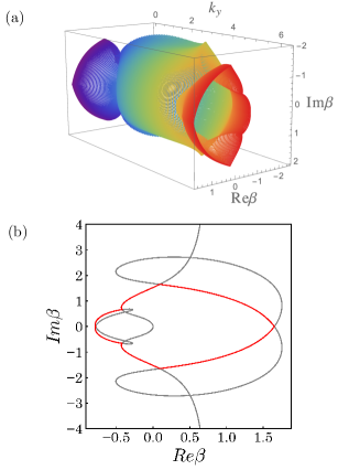
Figure 2: (a) An example of the generalized Brillouin zone surface (GBZ_s) for model $H_{3}$. It is a three-dimensional surface in the space $(\mathrm{Re}\beta,\mathrm{Im}\beta,k_{y})$, continuous but not necessarily smooth. Different values of $k_{y}\in[0,2\pi]$ are colored coded. (b) The cross section of the GBZ_s at $k_{y}=0$. The red curve is the GBZ showing numerous cusps. It consists of arc segments belonging to multiple auxiliary GBZ curves (in grey) which intersect with each other. Thus, the GBZ_s, in general is not a smooth manifold but an algebraic variety. The results are obtained numerically by following the algorithm outlined in Sec. II.C. The parameters used are $m=0.6$, and $t_{1}=0.4$.

In reality, carrying out this plan runs into difficulties. The GBZ surface is, in general, not a smooth compact manifold like the two-torus. This makes the definition and numerical computation of the Chern number challenging. Computing the GBZ curve for 1D non-Hermitian Hamiltonians is a nontrivial task. A few powerful algorithms have been developed so far Yokomizo and Murakami (2019); Yang et al. (2020); Wu et al. (2022), and they rely on numerical solution of algebraic equations (e.g., finding the roots of polynomial equations or the intersections of two curves) to yield a collection of discrete data points for $\beta$ on the complex plane. With sufficient resolution, these data points coalesce into a curve which is believed to be continuous and closed, but not necessarily smooth. In fact, it often has sharp turns, or cusps. An example is the red curve in Fig. 2(b). After running the algorithm for each $k_{y}\in[0,2\pi]$, the resulting GBZ_s inherits these cusps, see the example shown in Fig. 2(a).

To make matters worse, the resulting GBZ_s sometimes features singularities as $k_{y}$ is varied. For example, each GBZ curve of $H_{2}$ is a circle of radius $r$ on the complex plane, but $r$ shrinks to zero or blows up to infinity at certain $k_{y}$ values as shown in Fig. 3. Thus, to evaluate the Chern number from the Berry connection for a general non-Hermitian Chern insulator, we have to settle for irregular mesh points on a rugged GBZ_s, and watch out for singularities, e.g. when the GBZ surface shrinks to a point. Note that, previously, in Ref. Guo et al. (2021), the singularities of GBZ in 1D non-Hermitian models have been noted. Here, we focus on 2D models. To circumvent these subtleties and crosscheck the Chern number calculation, we shall also pursue an alternative scheme to characterize the topological invariant of ${\mathcal{H}}(\beta,k_{y})$ using the eigenvectors on the Bloch sphere.

From Secs, III-V, the three models $H_{1,2,3}$ are discussed, in turn, to illustrate the technical complexities and challenges in executing the strategy outlined above centering around $\mathcal{H}(\beta,k_{y})$ and GBZ_s. In particular, we show how analytical solutions can be obtained for $H_{2}$ to yield a thorough understanding of the problem. By working through these three examples, we hope the reader can appreciate the rich, nontrivial behaviors of non-Hermitian Chern insulators with open boundaries as highlighted in Fig. 1.

II Computing the GBZ

The concept of a GBZ plays a crucial role in our analysis of the non-Hermitian Chern insulators. In this section, we outline the technical procedures to compute the GBZ_s for our two-band models. Based on existing algorithms, we introduce a few tricks so the numerical task is simplified and analytical results become possible. This leads to a rather detailed knowledge of how the GBZ varies with the parameters such as $m$, $h_{x}$ or $t_{1}$, and $k_{y}$, including the development of singularities.

II.1 The algorithm

The first step of the algorithm is to analytically continue $H_{\text{bulk}}(k_{x},k_{y})$ by the replacement $e^{ik_{x}}\rightarrow\beta$. Take model $H_{2}(k_{x},k_{y})$ as an example. After the replacement, $H_{2}$ becomes

$$\mathcal{H}_{2}(\beta,k_{y}) = \big{(}ih_{x}+\frac{\beta-\beta^{-1}}{2i}\big{)}\sigma_{x}+\sin k_{y}\sigma_{y}$$ (13)

$$+\big{(}m-\cos k_{y}-\frac{\beta+\beta^{-1}}{2}\big{)}\sigma_{z}.$$

The two eigenvalues of $\mathcal{H}_{2}$ are $\pm E(\beta)$, where the $k_{y}$ dependence of $E$ has been suppressed for brevity. We will focus on their square, which is a Laurent polynomial of complex variable $\beta$:

$$\epsilon(\beta)\equiv{E}^{2}(\beta)=\frac{a^{\prime}\beta^{2}+b^{\prime}\beta+c^{\prime}}{\beta}.$$ (14)

Here the coefficients

$$a^{\prime} = -m+\cos k_{y}+h_{x},$$ (15)

$$b^{\prime} = m^{2}-2m\cos k_{y}+2-h_{x}^{2},$$ (16)

$$c^{\prime} = -m+\cos k_{y}-h_{x}.$$ (17)

For $\beta$ living on the unit circle with $|\beta|=1$, let $\beta=e^{ik_{x}}$ with $k_{x}\in[-\pi,\pi]$, then $\epsilon(\beta)$ becomes $\epsilon(k_{x})$ to reproduce the bulk spectrum Eq. (6), i.e., the spectrum of $H_{2}$ with periodic boundary conditions.

To discuss the slab geometry with open boundaries and the corresponding edge modes, let us write $H_{2}$ in second quantized form:

$$H_{2}=\sum_{n=1}^{L}\sum_{k_{y}}\left[\psi^{\dagger}_{n}A\psi_{n}+\psi^{\dagger}_{n}B\psi_{n+1}+\psi^{\dagger}_{n+1}C\psi_{n}\right].$$ (18)

Here the good quantum number $k_{y}$ is the crystal momentum along $y$, $n$ is the unit cell index along $x$, the creation operator $\psi^{\dagger}_{n}$ is a shorthand notation for the spinor $[\psi^{\dagger}_{n,\uparrow}(k_{y}),\psi^{\dagger}_{n,\downarrow}(k_{y})]$, and $A$, $B$, $C$ are $2\times 2$ matrices:

$$A = [m-\cos k_{y}]\sigma_{z}+ih_{x}\sigma_{x}+\sin k_{y}\sigma_{y},$$ (19)

$$B = (-\sigma_{z}+i\sigma_{x})/2,$$ (20)

$$C = B^{\dagger}.$$ (21)

Again, the $k_{y}$ dependence of $\psi_{n}$ and $A$ is suppressed for brevity. In other words, $H_{2}$ is a block Toeplitz matrix:

$$\mathcal{T}=\left[\begin{array}[]{ccccc}A&B&0&0&..\\ C&A&B&0&..\\ 0&C&A&B&..\\ ..&..&..&..&..\end{array}\right]_{L\times L}.$$ (22)

This form is particularly convenient for finding the dispersion and location of the edge states in Sec. IV.

We stress that the open spectrum (i.e., the set of eigenvalues of $\mathcal{T}$ for a system of size $L$ in the $x$ direction with open boundaries at $x=0,L$) may bear little similarity with the bulk spectrum $E_{\text{bulk}}(k_{x},k_{y})$ in Eq. (6). Furthermore, the open spectrum depends on the size $L$. And since $\mathcal{T}$ is non-Hermitian, its numerical diagonalization is prone to instabilities and large errors when $L$ is large. Some of these counterintuitive phenomena have been long noticed for non-Hermitian Toeplitz matrices (here we are dealing with block Toeplitz matrices). A simple example is when the three matrices $A$, $B$, and $C$ reduce to numbers with $A=0$. In this case, the bulk spectrum is an ellipse (a curve), while the open spectrum is a line segment within the ellipse. The sensitive dependence of the spectra on the boundary conditions has been well recognized for non-Hermitian Hamiltonians.

The spectra of $\mathcal{T}$ in the thermodynamic limit $L\rightarrow\infty$, save for a subset corresponding to the edge states, are called continuum bands. The eigenvalues of $\mathcal{T}$ congregate into continuum sets (e.g., lines) on the complex $E$ plane. And the corresponding eigenstates may include localized states that do not belong to the bulk spectrum with periodic boundaries. A key step in understanding the slab phase diagrams of non-Hermitian Chern insulators is to find the continuum bands. Remarkably, this task can be reduced to an algebraic problem involving the analytically continued Hamiltonian $\mathcal{H}(\beta)$. The eigenvalue problem of $\mathcal{H}(\beta)$ has the following generic form:

$$\frac{P_{p+q}(\beta,E)}{\beta^{p}}=0.$$ (23)

Here $P_{p+q}$ denotes a polynomial of $\beta$ of degree $p+q$ (it is also a polynomial of $E$ of some other degree). For example, in Eq. (14) for $\mathcal{H}_{2}$, we have $p=1$ and $q=1$. For generalized Qi-Wu-Zhang models, Eq. (23) can be further simplified to a form similar to Eq. (14),

$$\epsilon(\beta)=\frac{Q_{p+q}(\beta)}{\beta^{p}},$$ (24)

where $Q_{p+q}$ is a polynomial of $\beta$ of degree $p+q$ with coefficients independent of $E$. Equation (24) defines a mapping $\beta\rightarrow\epsilon$, i.e., from $\beta$ on the complex plane to $\epsilon=E^{2}$, which is also complex. Note that this is a multiple-to-one mapping: For a given image $\epsilon$, we label its preimages by $\beta_{i}$ and order them by their magnitudes:

$$|\beta_{1}|\leq|\beta_{2}|\leq...\leq|\beta_{p+q}|.$$ (25)

For $E$ to lie within the continuum band, its preimages $\beta_{p}$ and $\beta_{p+1}$ must satisfy the degeneracy condition:

$$|\beta_{p}|=|\beta_{p+1}|.$$ (26)

This key result was established in Refs. Yao and Wang (2018) and Yokomizo and Murakami (2019) for 1D non-Hermitian Hamiltonians. And in the context of Toeplitz matrices, it was first proved by Schmidt and Spitzer (see Theorem 1 of Ref. Schmidt and Spitzer (1960) and Refs. Beam and Warming (1991); Böttcher and Grudsky (2005) for a review). Solving Eq. (26) together with Eq. (24) accomplishes two goals at once: the set of $E$’s form the continuum band, and the union of the set $\beta_{p}$ and set $\beta_{p+1}$ gives the GBZ.

II.2 Circular GBZ for model $H_{2}$

Let us apply the algorithm to $H_{2}$ to show its GBZ is a circle. Recall from Eq. (14), $\epsilon(\beta)=a^{\prime}\beta+b^{\prime}+c^{\prime}/\beta$, so $p=1$ and each $\epsilon$ only has two preimages, $\beta_{1}$ and $\beta_{2}$. The degeneracy condition requires them to have equal magnitude, therefore we can follow the parametrization scheme of Ref. Yokomizo and Murakami (2019) to write

$$\beta_{2}=\beta_{1}e^{i\theta}.$$ (27)

Next, using $\epsilon(\beta_{1})=\epsilon(\beta_{2}=\beta_{1}e^{i\theta})$, we find

$$\beta^{2}_{1}=\frac{c^{\prime}}{a^{\prime}}e^{-i\theta}.$$ (28)

Thus the GBZ for $\mathcal{H}_{2}$ is a circle with radius

$$r_{2}(k_{y})=\left|\frac{m-\cos k_{y}+h_{x}}{m-\cos k_{y}-h_{x}}\right|^{1/2}.$$ (29)

We stress that working with $\epsilon=E^{2}$ is a simple yet crucial trick to render the problem analytically tractable.

Figure 3 shows two examples of the GBZ radius varying with $k_{y}$. It clearly illustrates the pinching of the GBZ_s where $r_{2}$ vanishes, as well as the divergence of $r_{2}$ at certain $k_{y}$ values dependent on the parameter $m$ and $h_{x}$.

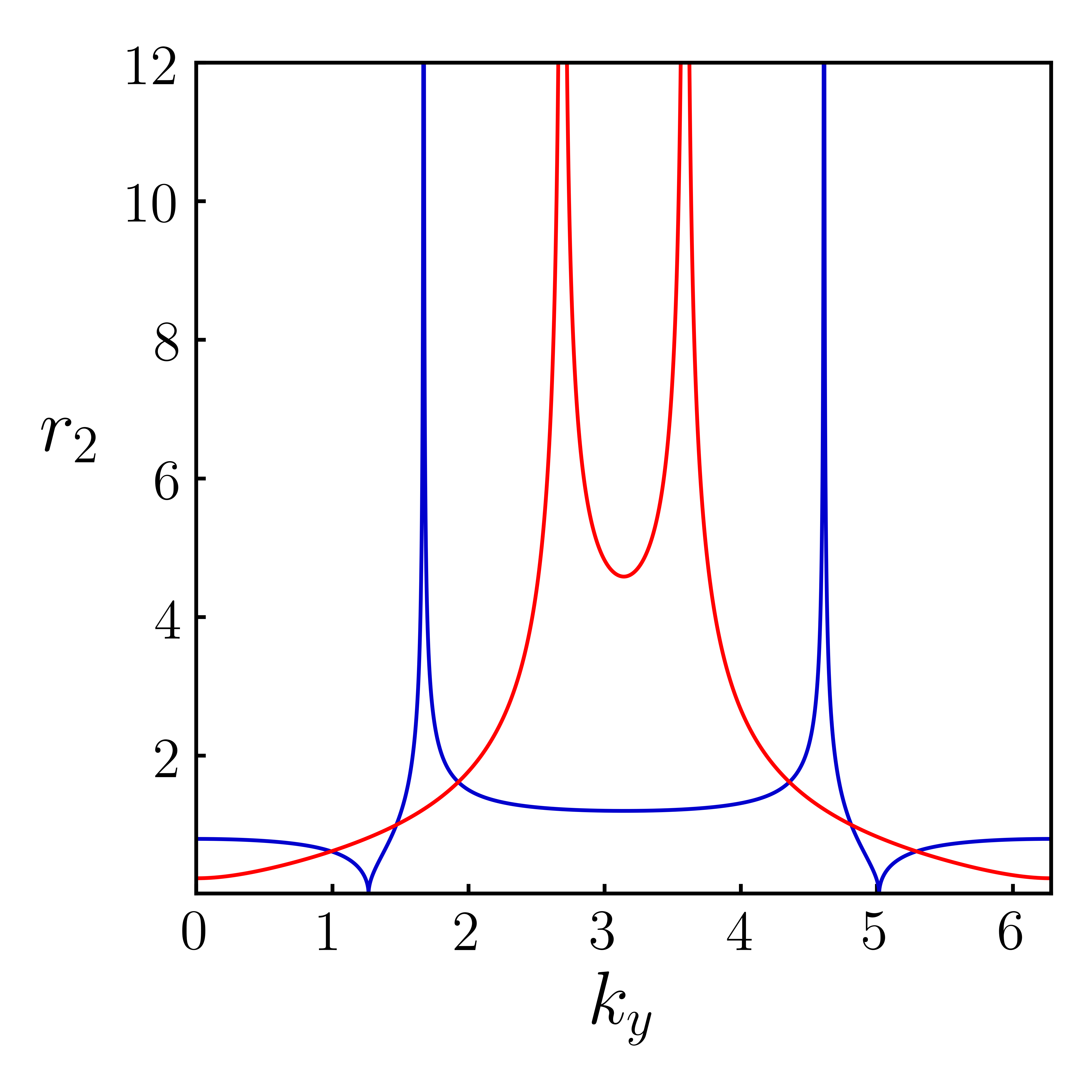
Figure 3: Singularities in the circular GBZ of model $H_{2}$. The radius $r_{2}$, given by Eq. (29), is plotted as a function of $k_{y}\in[0,2\pi]$ for $m=0.1$, $h_{x}=0.2$ (in blue), and for $m=0.1$, $h_{x}=1$ (in red). It shrinks to zero when $m-\cos k_{y}+h_{x}=0$, and blows up to infinity when $m-\cos k_{y}-h_{x}=0$.

II.3 GBZ for model $H_{3}$

Next we apply the algorithm to the analytically continued model $H_{3}$, which has the form

$$\mathcal{H}_{3}(\beta,k_{y}) = \frac{\beta-\beta^{-1}}{2i}\sigma_{x}+\sin k_{y}\sigma_{y}$$

$$+ \big{(}m-\cos k_{y}+\frac{1-t_{1}}{2}\beta-\frac{t_{1}+1}{2}\beta^{-1}\big{)}\sigma_{z}.$$

Its eigenvalue square is the Laurent polynomial

$$\epsilon(\beta)\equiv{E}^{2}(\beta)=a\beta^{2}+b/\beta^{2}+c\beta+d/\beta+f,$$ (31)

with

$$a = t_{1}(t_{1}-2)/4,$$ (32)

$$b = t_{1}(t_{1}+2)/4,$$ (33)

$$c = +(m-\cos k_{y})(t_{1}-1),$$ (34)

$$d = -(m-\cos k_{y})(t_{1}+1),$$ (35)

$$f = (m-\cos k_{y})^{2}+\sin^{2}k_{y}-t_{1}^{2}/2+1.$$ (36)

Comparing with the general form Eq. (24), we find that, in this case, $p=q=2$, so the degeneracy condition becomes

$$|\beta_{2}|=|\beta_{3}|.$$ (37)

This motivates the parametrization $\beta_{3}=\beta_{2}e^{i\theta}$. To find the GBZ, we need to solve the quartic equation

$$\epsilon(\beta_{2})=\epsilon(\beta_{2}e^{i\theta})$$ (38)

for $\beta_{2}$ for all possible values of $\theta$.

Before attempting a general solution, let us first consider a special case $m=1$ and $k_{y}=0$, so $c=d=0$. Then the Laurent polynomial Eq. (31) simplifies to $\epsilon(\beta)=a\beta^{2}+b/\beta^{2}+f$, and Eq. (38) can be solved by hand. After a little algebra, we find

$$\beta^{4}_{2}=\frac{t_{1}+2}{t_{1}-2}e^{-i2\theta}.$$ (39)

Thus, the GBZ for $m=1$ and $k_{y}=0$ is a circle of radius

$$r_{3}=\left|\frac{t_{1}+2}{t_{1}-2}\right|^{1/4}.$$ (40)

For general values of $(m,t_{1},k_{y})$, we choose to solve Eq. (38) numerically to find its four solutions $\eta_{i}$, $i=1,2,3,4$. For each solution $\eta_{i}$, we compute its image $\epsilon^{*}=\epsilon(\eta_{i})$, and find all four preimages of $\epsilon^{*}$ and sort them into

$$|\xi_{1}|\leq|\xi_{2}|\leq\xi_{3}|\leq|\xi_{4}|.$$ (41)

If $|\xi_{2}|=|\xi_{3}|$ and $\eta_{i}=\xi_{2}$ or $\xi_{3}$, we conclude that $\eta_{i}$ and $\eta_{i}e^{i\theta}$ satisfy the condition Eq. (37) and therefore belong to the GBZ. Repeating this procedure for a discrete grid of $\theta$ values within the interval $[0,2\pi]$ will produce a set of data points to form the GBZ curve [e.g., the red curve in Fig. 2(b)].

It is not immediately obvious that the GBZ obtained this way is guaranteed to be a connected, closed curve. To gain a better understanding, it is useful to examine all the solutions of Eq. (38), including those that do not meet the criterion Eq. (37) and thus do not belong to the GBZ. As the solutions of a polynomial equation, they forms continuous curves on the complex $\beta$ plane which are called the auxiliary GBZ by Ref. Yang et al. (2020). For example, some of the solutions satisfy $|\beta_{j}|=|\beta_{j+1}|$, with $j\neq q$. These curves may intersect, and GBZ is nothing but a subset of the auxiliary GBZ, consisting of arcs connected to each other at these intersection points. Figure 2 shows the computed GBZ (in red) and other auxiliary GBZ for parameters $m=0.6$, $t_{1}=0.4$ with $k_{y}=0$.

It is clear from the discussion above that the GBZ, unlike the familiar BZ, is not necessarily a smooth manifold and may feature singular points. More precisely, it should be called an algebraic variety, as it is derived from solutions to polynomial equations.

II.4 GBZ from self-intersection

The recipe outlined in the preceding subsections works very well in tracing out smooth GBZ curves, e.g., approximately of elliptical shape. Its performance suffers, however, when the GBZ contains segments going along the radial direction, which can be easily missed if the mesh grid of $\theta$ is not fine enough. Thus, it is useful to develop an alternative method that can find points on the GBZ at a given radius $\rho$ on the complex $\beta$ plane. An ingenious algorithm of this type was proposed in Ref. Wu et al. (2022) based on the self-intersection and winding of the image $\epsilon(\beta)$. Below, we show how it can be adapted to $\mathcal{H}_{3}$. Readers who are not interested in these technical details can skip to Sec. III.

Let $\mathscr{C}_{\rho}$ be a circle of given radius $\rho$ on the complex plane. As $\beta$ varies along $\mathscr{C}_{\rho}$ to complete a cycle, its image $\epsilon(\beta)$ traces out a closed curve $\Gamma_{\rho}$ on the complex plane of $\epsilon$:

$$\Gamma_{\rho}=\left\{\epsilon(\beta\in\mathscr{C}_{\rho})\right\}.$$ (42)

Thus, for two distinct points $\beta_{i}$ and $\beta_{j}$ on $\mathscr{C}_{\rho}$ to map to the same image $\epsilon_{s}\in\Gamma_{\rho}$,

$$\epsilon(\beta_{i}\in\mathscr{C}_{\rho})=\epsilon(\beta_{j}\in\mathscr{C}_{\rho})=\epsilon_{s},$$ (43)

$\epsilon_{s}$ must be a self-intersection points of the curve $\Gamma_{\rho}$. For our problem, we observe that the location of these points are mirror symmetric with respect to the real axis, because all coefficients $a$ to $f$ in Eq. (31) are real.

Plotting the curve $\Gamma_{\rho}$ reveals that it is, in general, very complicated. One may take a purely numerical approach to find its intersection points. But it is time consuming (we must repeat the calculation for different $\rho$’s and different parameters such as $k_{y}$) and requires fine-tuning for different parameters. It turns out that with some effort all the self-intersection points for model $\mathcal{H}_{3}$ can be found analytically as follows. For a given radius $\rho$, let us parametrize $\beta=\rho e^{i\theta}$ and separate $\epsilon$ into real and imaginary parts, $\epsilon(\beta=\rho e^{i\theta})=x(\theta)+iy(\theta)$. Then Eq. (31) becomes two equations,

$$x(\theta)=a_{+}\cos 2\theta+c_{+}\cos\theta,$$ (44)

$$y(\theta)=a_{-}\sin 2\theta+c_{-}\sin\theta,$$ (45)

with the shorthand notation

$$a_{\pm} =a\rho^{2}\pm{b}{\rho^{-2}},$$ (46)

$$c_{\pm} =c\rho\pm{d}{\rho^{-1}}.$$ (47)

According to Eq. (43), a self-intersection point of $\Gamma_{\rho}$ corresponds to a solution to the equation set

$$x(\theta)=x(\theta^{\prime}),$$ (48)

$$y(\theta)=y(\theta^{\prime}),$$ (49)

with $\theta\neq\theta^{\prime}$. These trigonometric equations can be converted into polynomial form by introducing

$$u=\cos\theta,\;\;\;v=\cos\theta^{\prime},$$ (50)

and applying trig identities. For example, Eq. (48) for $x$ reduces to

$$u+v=-c_{+}/2a_{+}$$ (51)

after factoring out $(u-v)$. Eq. (49) for $y$ is more involved. One can square it to obtain a quartic equation for $u$ and $v$ using $\sin^{2}\theta=1-u^{2}$. Luckily, we can factor out $(u-v)$ again, and evoke Eq. (51) to reduce it to a quadratic equation for $u$,

$${a}_{u}u^{2}+{b}_{u}u+{c}_{u}=0,$$ (52)

where the coefficients have lengthy expressions

$$\eta=-c_{+}/2a_{+},$$

$${a}_{u}=8a_{-}^{2}\eta+4a_{-}c_{-},$$

$${b}_{u}=-8a_{-}^{2}\eta^{2}-4a_{-}c_{-}\eta,$$

$${c}_{u}=4a_{-}^{2}\eta^{3}+4a_{-}c_{-}\eta^{2}+(c_{-}^{2}-4a_{-}^{2})\eta-4a_{-}c_{-}.$$

The quadratic Eq. (52) yields a pair of solutions $u_{\pm}$. Another independent solution of Eq. (49) corresponds to $y(\theta)=y(\theta^{\prime})=0$, leading to

$$u_{3}=-c_{-}/2a_{-},$$ (53)

with the corresponding intersection point lying on the real axis. For each solution of $u$, we can work backwards to find $\theta=\arccos(u)$, $v$, $\theta^{\prime}$, and $\epsilon_{s}=x(\theta)+iy(\theta)$.

In some special cases, the self-intersection points coincide and merge into a single point. This corresponds to having three $\beta$’s on the circle $\mathscr{C}_{\rho}$ that map to the same value of $\epsilon$. In Ref. Wu et al. (2022) this is called three-bifurcation point. Let the three $\beta$’s be $\beta_{1}=\rho_{c}$, $\beta_{2}=\rho_{c}e^{i\theta}$, and $\beta_{3}=\rho_{c}e^{-i\theta}$. They are the solutions of the quartic equation:

$$a\beta^{4}+c\beta^{3}-\epsilon\beta^{2}+d\beta+b=0.$$ (54)

Using Vieta’s formulas, after eliminating $\theta$, we find $\rho_{c}$ is the solution of a high order equation

$$a^{2}\rho_{c}^{8}+ad\rho_{c}^{5}-cb\rho_{c}^{3}-b^{2}=0,$$ (55)

which can be solved numerically, e.g., using MATHEMATICA. Once $\rho_{c}$ is known, $\theta$ can be found via

$$\cos\theta=-\frac{1}{2}(\rho_{c}^{4}a/b+\rho_{c}d/b+1).$$ (56)

This example illustrates the modest algebraic price one has to pay to understand the continuum bands of non-Hermitian Chern insulators. To summarize, the self-intersection points $\epsilon_{s}$ can be found analytically from the values of $a,b,c,d$, and $\rho$, except for solving Eq. (55) for the special case of higher-order bifurcation points.

Not all the self-intersection points $\epsilon_{s}$ found above belong to the continuum band. Reference Wu et al. (2022) established a qualifying criterion: The neighborhood of $\epsilon_{s}$ is divided into four regions by the two intersecting lines at $\epsilon_{s}$; with respect to a chosen point $\epsilon_{w}$ in one of these regions and away from $\Gamma_{\rho}$, the winding number of the curve $\Gamma_{\rho}$ defined by

$$W(\epsilon_{w})=\frac{1}{2\pi}\int_{\Gamma_{\rho}}dz\mathrm{Arg}(z-\epsilon_{w})$$ (57)

should be $+1,0,-1,0$ respectively. (The patterns of the winding number near a higher-order birfurcation points are more complicated and discussed in Ref. Wu et al. (2022)). The winding number is easy to evaluate numerically with the help of the argument principle,

$$W(\epsilon_{w})=N_{w}-p,$$ (58)

where $p=2$ and $N_{w}$ is the number of the preimages of $\epsilon_{w}$ residing inside the circle $\mathscr{C}_{\rho}$. For those qualified self-intersection points with the right set of winding numbers, we collect their preimages $\rho e^{i\theta}$ on the circle $\mathscr{C}_{\rho}$ as a subset of GBZ. By changing the radius $\rho$ and repeating the procedure, one obtains the whole GBZ curve.

What about those rejected $\epsilon_{s}$ with the “wrong” winding number patterns? Their preimages are nothing but the auxiliary GBZ. The self-intersection method described here is complementary to the scheme given in the preceding subsections. It excels at resolving the cusps where the other method struggles. We have checked that these two methods agree with each other and produce the same GBZ as well as the auxiliary GBZ.

III Exceptional ring of model 1

Some non-Hermitian Chern insulators are adiabatically connected to the familiar Hermitian Chern insulators. One example is the model $H_{1}$ defined in Eq. (2) by replacing $m$ with a complex Dirac mass $m+ih_{z}$ in the Qi-Wu-Zhang model $H_{0}$. In this case, the bulk-edge correspondence holds as usual, and there is no need for introducing the notion of the GBZ. The other two models $H_{2,3}$, in comparison, will not be so cooperative. Model $H_{1}$ provides a nice geometric picture of the band topology in terms of the $\mathbf{d}$ vectors. Here we show that the phase diagram of $H_{1}$ on the $(m,h_{z})$ plane [Fig. 1(a)] can be understood quantitatively by analyzing the the singularity of $H_{1}$ in the space of $\mathbf{d}$. This viewpoint based on the $\mathbf{d}$ vectors was advocated in Ref. Li et al. (2019) for a more complicated model.

As $k_{x}$ and $k_{y}$ vary throughout the BZ, the vector $\mathbf{d}(k_{x},k_{y})$ defined in Eq. (1) traces out a closed surface in the space of $(d_{x},d_{y},d_{z})$. The surface is mirror symmetric with respect to the plane $d_{z}=m$, where it becomes pinched along the diagonal lines $|d_{x}|=|d_{y}|\in[0,1]$. It is useful to imagine the upper half of the surface as a bloated tent of height 2 with its bottom stitched together along two lines on the ground. The eigenvalues of $H_{1}(k_{x},k_{y})$ will vanish when

$$d_{x}^{2}+d_{y}^{2}+(d_{z}+ih_{z})^{2}=0.$$ (59)

And the singularity here is an exceptional point. Separating the real and imaginary parts, we find the condition becomes

$$d_{z}=0,\;\;\;\;d_{x}^{2}+d_{y}^{2}=h_{z}^{2}.$$ (60)

This defines a ring of radius $h_{z}$ on the plane of $d_{z}=0$. We will call it the exceptional ring (Ref. Li et al. (2019) uses the more generic name “singularity ring”). In the limit of $h_{z}=0$, the Qi-Wu-Zhang model is recovered, and the ring shrinks to a point at the origin which, since the work of Berry Berry (1984), is often called a magnetic monopole carrying magnetic charge. In this sense, the ring here is a ring of magnetic charge.

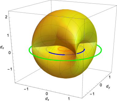
Figure 4: The ring and the tent: Geometric visualization of the $\mathbf{d}$ vector (golden surface, the tent) and the exceptional ring, Eqs. (60), for model $H_{1}$. At fixed $m=0.25$, for $h_{x}=0.3$, the exceptional ring (red) resides inside the tent, the system is within the topological phase C₁. For $h_{x}=0.8$, the ring (blue) intersects the tent surface, the system is gapless. For $h_{x}=1.5$, the ring is outside the tent, the system is gapped but topologically trivial. The base of the tent is at $m=0.25$.

Now the phase diagram of model $H_{1}$ can be worked out from the geometries of the tent (centered at $d_{z}=m$ with overall height $2|m|$) and the exceptional ring (centered around $d_{z}=0$ with radius $h_{z}$), see Fig. 4. When the exceptional ring lives inside/outside the tent, the system is a topologically nontrivial/trivial insulator; when the ring intersects the tent, the spectrum is gapless. Figure 1(a) shows the phase diagram of $H_{1}$ where the two gapped phases are separated by the gapless region. By examining the cross section of the tent surface with the $d_{z}=0$ plane and how it touches the ring, one can determine the phase boundaries. For example, for $m=1$ the lower critical point is at $h_{z}=1$ and the upper critical point is at $h_{z}=\sqrt{3/2}$. At $m=0$, the transition to the trivial gapped phase occurs at $h_{z}=2$. And the gap closes at $m=2$ and $h_{z}=0$. One can check that the edge states have real energy, and the bulk-edge correspondence holds for $H_{1}$.

IV Analytical theory of Model 2

In this section, we revisit the phases and edge modes of $H_{2}$, which has been investigated numerically in Ref. Kawabata et al. (2018). As discussed in the Introduction, our goal here is to achieve an analytical understanding. To this end, we shall restrict our focus to the first quadrant of the $(m,h_{x})$ plane with $m,h_{x}>0$. The phase diagram in other quadrants can be obtained by using symmetry. In particular, we establish the following eight theorems.

Theorem 1. The GBZ for model $\mathcal{H}_{2}(\beta,k_{y})$ defined in Eq. (13) is a circle of radius $r_{2}$ given by Eq. (29).

Theorem 2. The band structure of $\mathcal{H}_{2}(\beta\in\mathrm{GBZ},k_{y})$ defines three topologically nontrivial phases with robust edge states. Phase C₁ (C₂) has line gap and band Chern number $\pm 1$ ($\pm 2$), while phase S is gapless. The phase boundaries shown in Fig. 1(b) are given by four curves on the $(m,h_{x})$ plane,

$$m =\sqrt{1+h^{2}_{x}}+1,$$ (61)

$$m =\sqrt{1+h^{2}_{x}}-1,$$ (62)

$$h_{x} =\sqrt{(m-1)^{2}+1},$$ (63)

$$h_{x} =\sqrt{(m+1)^{2}+1}.$$ (64)

They mark the closing of the gap in the continuum band.

Theorem 3. In the thermodynamic limit $L\rightarrow\infty$, one of the edge modes of $H_{2}$ has dispersion

$$E^{+}_{\text{edge}}(k_{y})=+\sin k_{y},$$ (65)

with decay factor [defined in Eq. (78) below]

$$\lambda_{+}=m-\cos k_{y}-h_{x}.$$ (66)

In slab geometry, it is localized on the left (right) edge if $|\lambda_{+}|<1$ ($>1$).

Theorem 4. The other edge mode has dispersion

$$E^{-}_{\text{edge}}(k_{y})=-\sin k_{y},$$ (67)

with decay factor

$$\lambda_{-}=m-\cos k_{y}+h_{x}.$$ (68)

It is localized on the right (left) edge if $|\lambda_{-}|<1$ ($>1$).

Theorem 5. Phase C₁ is further partitioned into three regions (RR, LR, LL) based on the localization of the two edge modes near $k_{y}=0$. For example, in the LR region, the $E^{+}$ mode is localized on the left (L) edge, while the $E^{-}$ mode is localized on the right (R) edge. These three regions are separated by two lines:

$$m =h_{x},$$ (69)

$$m+h_{x} =2.$$ (70)

These lines do not correspond to gap closing. Rather, they mark the divergence of the localization length, i.e., $|\lambda_{\pm}|=1$, at $k_{y}=0$.

Theorem 6. In phase C₂, there are four edge modes at zero energy. Among them, $E^{\pm}(k_{y}=\pi)$ are localized on the left edge, while $E^{\pm}(k_{y}=0)$ are localized on the right edge.

Theorem 7. Phase S is gapless with two edge modes localized on the left edge and crossing $E=0$ at $k_{y}=\pi$.

Theorem 8. The energy eigenvalues of $\mathcal{H}_{2}$ are real for $m+\cos k_{y}>h_{x}$. For example, phase T at the bottom right corner of Fig. 1(b) has a real spectrum.

Taken together, these eight theorems provide a clear characterization of the phases and the edge modes of model 2. These analytical results agree with the numerical diagonalization of $H_{2}$ for large $L$ in slab geometry found in Ref. Kawabata et al. (2018). Below, we prove these theorems, and present a more detailed discussion of the phase diagrams, edge modes, and topological invariants.

IV.1 Continuum bands

Theorem 1 has been proved back in Sec. II.B. Since the GBZ is a circle, $\beta$ $\in$ GBZ can be parametrized by introducing a wave vector $\tilde{k}_{x}$:

$$\beta=r_{2}e^{i\tilde{k}_{x}},\;\;\;\;\tilde{k}_{x}\in[-\pi,\pi].$$ (71)

Then the continuum bands of $\mathcal{H}_{2}(\beta,k_{y})$ can be found from Eq. (13). After a little algebra, we find

$$E_{c}^{2}(\tilde{k}_{x},k_{y}) = 1+m_{y}^{2}-h_{x}^{2}+(h_{x}r_{-}-m_{y}r_{+})\cos\tilde{k}_{x}$$ (72)

$$+ \sin^{2}k_{y}+i(h_{x}r_{+}-m_{y}r_{-})\sin\tilde{k}_{x},$$

where the shorthand notation

$$m_{y} = m-\cos k_{y},$$ (73)

$$r_{\pm} = r_{2}\pm r_{2}^{-1}.$$ (74)

In general, the eigenenergy $E_{c}$ is complex according to Eq. (72). Within the region $m_{y}>h_{x}$, however, $h_{x}r_{+}-m_{y}r_{-}=0$ and therefore $E^{2}_{c}$ is real. By direct calculation, one can further show $E^{2}_{c}>0$ which proves Theorem 8.

Inspecting the continuum band structure confirms that phase C₁ and C₂ have a line gap, while phase S is gapless. Figure 5 gives two examples of the continuum bands (in color blue) for phases C₁ and C₂, respectively. It is illuminating to compare the continuum band $E^{2}_{c}$ above with the bulk spectrum: of $H_{2}(k_{x},k_{y})$,

$$E^{2}_{\text{bulk}}(k_{x},k_{y}) = 1+m_{y}^{2}-h_{x}^{2}-2m_{y}\cos k_{x}$$ (75)

$$+ \sin^{2}k_{y}+i2h_{x}\sin k_{x}.$$

This result clearly illustrates the highly nontrivial reconstruction of the band structure in many non-Hermitian Chern insulators, $E^{2}_{b}\rightarrow E^{2}_{c}$, as the boundary conditions change from periodic to open along the $x$ direction. In Fig. 5, the bulk spectra (in color red) obviously deviate from the corresponding continuum bands (in blue). For example, in phase C₂ one would expect the system to be gapless from the bulk dispersion, but instead the continuum band in the slab geometry develops a line gap, giving rise to a novel phase C₂. Such band reconstruction is responsible for much of the rich behaviors of non-Hermitian Chern insulators in the slab geometry.

Let us find out when the gap closes from the expression of $E^{2}_{c}(\tilde{k}_{x},k_{y})$. First, consider $k_{y}=0$, so $m_{y}=m-1$. For the case of $m_{y}>h_{x}$, let $z=\sqrt{m_{y}^{2}-h^{2}_{x}}$, then

$$E_{c}^{2}=1+z^{2}-2z\cos\tilde{k}_{x}.$$ (76)

Obviously, $E_{c}^{2}=0$ requires $\cos\tilde{k}_{x}=1$ so the solution is $z=1$, i.e., $m_{y}^{2}-h^{2}_{x}=1$ leading directly to Eq. (61). For the opposite case $m_{y}<h_{x}$, the gap touches down at $\tilde{k}_{x}=0$ or $\pi$ with

$$E_{c}^{2}=(m_{y}\pm r_{+}/2)^{2}-(h_{x}\pm r_{-}/2)^{2}.$$ (77)

Thus $E_{c}^{2}=0$ leads to, after a little algebra, $h^{2}_{x}=m_{y}^{2}+1$ which gives Eq. (63). Similarly, the gap may close at $k_{y}=\pi$ with $m_{y}=m+1$ instead. Running the calculation again for $m_{y}>h_{x}$, we are led to Eq. (62), while for $m_{y}<h_{x}$, the result is Eq. (64). Now we have found all the phase boundaries summarized in Theorem 2.

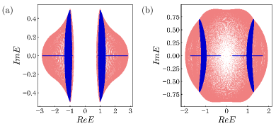
Figure 5: Deviation of the continuum band spectrum (blue) from the bulk spectrum (red) for model $H_{2}$. (a) Phase C₁ with $m=0.9$, $h_{x}=0.5$. (b) Phase C₂ with $m=0.15$, $h_{x}=0.9$. Notice the opening of the line gap in case (b) and the dramatic reconstruction of the band structure (red$\rightarrow$blue) as the boundary conditions change.

IV.2 Edge modes

Theorems 3 and 4 are not new results. The edge dispersions Eqs. (65) and (67) were established previously in Ref. Kawabata et al. (2018). For completeness, we briefly recount the derivation here. This serves three purposes. First, it clarifies the origin of the analytical expression for $\lambda_{\pm}$ which we will use to establish Theorems 5-7. Second, we will apply the same approach to model 3 in the next section, where the calculation becomes more challenging. Third, we find it fascinating that sinusoidal edge dispersion emerges not only for models $H_{2}$ and $H_{3}$ (see Sec. V.B) but also for some driven quantum Hall systems Satija and Zhao (2016). Thus, it is worthwhile to review the main arguments.

Consider a semi-infinite system ($x\geq 0$) with an open boundary at $x=0$ (the left edge) described by the matrix $\mathcal{T}$ in Eq. (22) with $L\rightarrow\infty$. Seeking a solution for the edge state, we try the ansatz

$$\psi=(\phi,\lambda\phi,\lambda^{2}\phi,...)^{T},$$ (78)

where $\lambda$ is referred to as the decay factor, $\phi$ is a two-component spinor and $(...)^{T}$ means transpose. In terms of the $2\times 2$ matrices $A,B,C$ defined in Eqs. (19) to (21), the eigenvalue problem $\mathcal{T}\psi=E\psi$ reduces to

$$\left[A+B\lambda\right]\phi = E\phi,$$ (79)

$$\left[C\lambda^{-1}+A+B\lambda\right]\phi = E\phi.$$ (80)

Following Ref. Kawabata et al. (2018), we conclude that $C\phi=0$, and $\phi=(1,i)^{T}/\sqrt{2}$. Plugging $\phi$ back into Eq. (79), we are facing the following dilemma:

$$(m-\cos k_{y}-\lambda-h_{x})\phi^{*}=(E-\sin k_{y})\phi.$$ (81)

The only way for this equation to hold is for the two coefficients in the parenthesis to vanish. This proves Eqs. (65) and (66).

Note the energy of the edge state is always real, and crosses zero at $k_{y}=0$ or $\pi$. Let us examine the spatial profile of this edge mode near $k_{y}=0$. It is localized on the left edge if the wave function decays with increasing $x$, that is, if $|\lambda|<1$. According to Eq. (66), this occurs within the strip $h_{x}<m<2+h_{x}$ (recall we only focus on the first quadrant $m,h_{x}>0$). Outside this region on the $(m,h_{x})$ plane, $|\lambda|>1$ so the solution $E^{+}$ describes a mode that grows with $x$, i.e., localized on the right edge. (In the slab geometry, an edge mode on the right edge still needs to satisfy the open boundary condition at $x=0$.)

The other edge mode solution can be worked out analogously by considering a semi-infinite system occupying $x\leq 0$, with an open boundary on the right edge $x=0$. In this case, we seek solution of the type

$$\psi=(...,\lambda^{2}\phi,\lambda\phi,\phi)^{T},$$ (82)

with

$$\left[C\lambda+A\right]\phi = E\phi,$$ (83)

$$\left[C\lambda+A+B\lambda^{-1}\right]\phi = E\phi.$$ (84)

By repeating the argument in the preceding paragraph, it is straightforward to show Eqs. (67) and (68). At $k_{y}=0$, we find that when $m+h_{x}<2$, $|\lambda|<1$, i.e., the edge state is localized on the right edge. Otherwise, the solution represents a state on the left edge. Note that in the discussion above, we have implicitly assumed the continuum band structure has a gap at $k_{y}=0$. Otherwise, the solution does not qualify as an edge state.

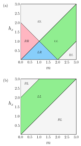
Figure 6: The localization phase diagrams for the edge modes of model $H_{2}$ near (a) $k_{y}=0$ and (b) $k_{y}=\pi$. The first (second) capital letter indicates the localization of the $E^{+}$ ($E^{-}$) edge mode. Combining these results with the phase boundary in Theorem 2 fixes the phase diagram of model $H_{2}$ in Fig. 1(b). See main text for details.

These results regarding the location of the edge modes near $k_{y}=0$ can be combined to yield the “localization phase diagram” shown in Fig. 6(a). We can identify four regions on the $(m,k_{y})$ plane: LL, RR, LR, and RL. Here the first capital letter indicates whether the $E^{+}(k_{y}\sim 0)$ mode resides on the left (L) or right (R) edge, while the second letter describes the location of the $E^{-}(k_{y}\sim 0)$ mode. In particular, the RR, LR, and LL regions are separated by two lines, $m=h_{x}$ and $m+h_{x}=2$, where $|\lambda_{\pm}|=1$. This proves Theorem 5.

The edge states $E^{\pm}$ also cross zero energy at $k_{y}=\pi$ inside phase C₂ and phase S. From the expression for $\lambda_{+}$ in Eq. (66), we conclude that $E^{+}(k_{y}\sim\pi)$ is localized on the left edge for $m<h_{x}<m+2$. Similarly, from $\lambda_{-}$, we find that $E^{-}(k_{y}\sim\pi)$ is always localized on the left edge in the first quadrant. The resulting “localization phase diagram” for the edge modes near $k_{y}=\pi$ is summarized in Fig. 6(b). If we overlay Figs. 6(a) and 6(b), we are led to Theorem 6: Inside phase C₂, the two modes $E^{\pm}(k_{y}\sim 0)$ are within the region of RR, while $E^{\pm}(k_{y}\sim\pi)$ are within the region of LL. In other words, out of the four edge modes crossing the zero energy, two of them are on the left edge, and the other two are on the right edge. We stress once again that such a scenario is only possible in non-Hermitian Chern insulators.

IV.3 Chern number

To characterize all gapped phases of model $H_{2}$, we compute the Chern numbers. The starting point is the analytically continued, non-Hermitian Hamiltonian $\mathcal{H}_{2}(\beta,k_{y})$ in Eq. (13) with $\beta=r_{2}(k_{y})e^{i\tilde{k}_{x}}\in\mathrm{GBZ}$. The left and right eigenstates of $\mathcal{H}_{2}$ are defined as

$$\mathcal{H}_{2}\ket{\psi_{\ell}}=E_{\ell}\ket{\psi_{\ell}},$$ (85)

$$\bra{\xi_{\ell}}\mathcal{H}_{2}=\bra{\xi_{\ell}}E_{\ell}.$$ (86)

Here $\ell=\pm$ is the band index, and the dependence on $(\beta,k_{y})$ is suppressed. The right eigenstates $\left\{\ket{\psi_{\ell}}\right\}$ are linearly independent but not necessarily orthogonal Brody (2013). Instead, we require them to satisfy the biorthogonal normalization condition, $\braket{\xi_{\ell}}{\psi_{\ell^{\prime}}}=\delta_{\ell,\ell^{\prime}}$. The (generalized) Chern number is defined as an integral of the Berry curvature over the GBZ surface,

$$C_{\ell}=\frac{1}{2\pi i}\int_{\mathrm{GBZ}_{s}}d\tilde{k}_{x}dk_{y}\epsilon^{ij}\partial_{i}\bra{\xi_{\ell}}\partial_{j}\ket{\psi_{\ell}}.$$ (87)

Here $i,j=\tilde{k}_{x},k_{y}$ are the two independent directions on the GBZ surface, with repeated indices summed over.

According to Eq. (29), the GBZ curve as a circle shrinks to a dot ($r_{2}=0$) when $\cos k_{y}=-(m+h_{x})$ and the radius $r_{2}$ diverges when $\cos k_{y}=-(m-h_{x})$. Thus, rigorously speaking, the Berry curvature becomes ill defined at these singular points of $k_{y}$. To yield a sensible result, the integral in Eq. (87) must be understood as the principal value. An efficient, gauge-invariant way to numerically evaluate the Chern number is to partition the BZ into little patches and find the flux through each patch, e.g., by taking the trace of the Berry connection along the boundary of the patch Fukui et al. (2005). This algorithm can be generalized to compute the Chern number over the GBZ_s, as long as one carefully avoids hitting the singular points along the patch boundaries. To understand why this procedure works, imagine continuously deforming the GBZ_s only at the vicinity of these singularities so it becomes closed and smooth, leaving the patch boundary intact. Thanks to Gauss’s theorem, the total flux stays the same during the deformation, as long as the small deformation does not encounter any magnetic charge. Then, the Chern number calculated on the deformed smooth GBZ_s is well-defined, and has the same value as the original GBZ_s with integrable singularities. We find the resulting Chern number for phase C₁ (C₂) is $\pm 1$ ($\pm 2$), which completes the proof of Theorem 2.

To cross-check the numerical calculation of the Chern number, we adopt a complementary scheme to visualize and characterize the topology of the gapped phases. The eigenvalue problem of $\mathcal{H}_{2}$ in Eq. (85) defines a mapping from the GBZ_s to the Bloch sphere once the eigenvector of $\mathcal{H}_{2}$ is parametrized using the polar angle $\theta$ and the azimuthal angle $\phi$,

$$(\beta,k_{y})\in\mathrm{GBZ}_{s}\mapsto|\psi\rangle=e^{i\chi}\left(\begin{array}[]{c}\cos\frac{\theta}{2}\\ \sin\frac{\theta}{2}e^{i\phi}\end{array}\right),$$ (88)

with $\chi$ the overall phase. Then one can define the Chern number as the number of times the images of $(\beta,k_{y})$ cover the whole Bloch spheres as it varies throughout the GBZ_s. Figure 7 shows the wrapping for phases C₁ and C₂. They agree with the numerical integration results above. This approach circumvents the subtleties regarding Berry curvature near the singular points of GBZ. Interestingly, it also provides a geometric picture of these singularities. Direct analytical calculation reveals that, at these singular points, the eigenstates lie within the equator of the Bloch sphere. More specifically, $r_{2}\rightarrow 0$ and $\infty$ corresponds to the eigenvector pointing along the $\mp y$ axis, respectively, i.e., $\theta=\pi/2$ and $\phi=\mp\pi/2$. These two points are visible in Fig. 7 as the center of the small concentric red and blue rings.

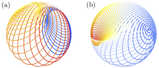
Figure 7: Counting the Chern number by the wrapping of eigenvectors of model $H_{2}$ on the Bloch sphere. (a) Phase C₁ with $m=1.5$, $h_{x}=0.3$. Different colors correspond to a discrete set of $k_{y}$ values from $0$ to $2\pi$, while the data points of the same color depict varying $\tilde{k}_{x}$ for a given $k_{y}$. As $(\tilde{k}_{x},k_{y})$ transverse the entire GBZ_s, the eigenvector covers the Bloch sphere exactly once. (b) Phase C₂ with $m=0$, $h_{x}=1$. Here only $k_{y}$ values restricted to $[0,\pi]$ are shown, and they are sufficient to cover the whole Bloch sphere. Thus, the Chern number is two. In the trivial phase T (not shown), the eigenvectors cannot cover the entire Bloch sphere.

IV.4 The gapless phase S

Phase S is gapless, and it has no analog in Hermitian Chern insulators. When the spectrum (in slab geometry) is plotted on the complex energy plane, there is no line gap (but there is a point gap around $E=0$). The continuum band spectrum in Fig. 8(a) forms a single connected surface with “holes” in the space of $(\mathrm{Re}E,\mathrm{Im}E,k_{y})$. The finite-size spectrum in Fig. 8(b) clearly shows a pair of edge states crossing $E=0$ at $k_{y}=\pi$ as described by Eqs. (65) and (67). From the localization phase diagram of these modes in Fig. 6(b), it is clear that both modes localize on the left edge, which proves Theorem 7 and is confirmed by numerical results. Note the good agreement between Figs. 8(a) and 8(b) for $L=50$. For large $L$, the diagonalization of the non-Hermitian Hamiltonian is prone to numerical instabilities, and the resulting spectrum starts to show large fluctuations due to numerical error and then becomes unreliable. This further reinforces the usefulness of the GBZ and the analytical approach we advocate here which operates directly in the $L\rightarrow\infty$ limit.

In passing, we mention that in the phase diagram Fig. 1(b), the trivial region T at the bottom-right corner has a line gap and real spectrum. In comparison, the spectrum of the T region at the left top corner is complex. The region GL is gapless, there are edge modes but they do not cross zero energy. To summarize, analytical results obtained for $\mathcal{H}_{2}$ in this section capture all the main features of the phase diagram, edge states, and topological characterization of each gapped phase. This example illustrates the capability as well as the subtleties of this approach based on the GBZ. We will apply the approach to another in the next section.

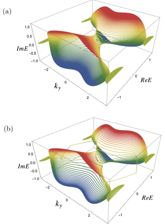
Figure 8: The gapless phase S of model $H_{2}$. (a) The continuum band spectrum from analytical calculation. (b) Spectrum from numerical diagonalization of a slab with $L=50$, showing a pair of edge states crossing $E=0$ at $k_{y}=\pi$. Both are localized at the left edge. $m=0.3$, $h_{x}=1.25$.

V Model 3

In this section, we analyze $H_{3}$, the third model of non-Hermitian Chern insulators defined in Eq. (4). Compared to model $H_{1}$ and $H_{2}$ above, this model introduces a unique feature: the hopping between neighboring unit cells is non-reciprocal. More specifically, the intra-orbital hopping amplitudes to the left and right are given by $1+t_{1}$ and $1-t_{1}$ respectively. The finite $t_{1}$ term makes it more challenging to find the GBZ, the continuum band structure, the phase diagram, and the edge states. But these tasks are still manageable thanks to the techniques developed in Secs. II and IV.

For the sake of clarity, we summarize our main results into Theorems 9-13 below. Hereafter, the term phase diagram refers to the phase diagram for model 3 in slab geometry (with open boundaries at $x=0,L$ and periodic boundary conditions along $y$) in the limit of $L\rightarrow\infty$, and we shall restrict our attention to the first quadrant of the parameter space, $m,t_{1}>0$. It is straightforward to generalize the analysis to other parameter regions.

Theorem 9. For $k_{y}=0$, the GBZ is a circle on the complex $\beta$ plane with radius $r_{3}$ given by Eq. (40).

Theorem 10. The phase diagram of $H_{3}$ is mirror symmetric with respect to $m=1$. It consists of six regions shown in Fig. 1(c). The continuum bands of phase T have a line gap and are topologically trivial (i.e., their Chern numbers are zero). Region C${}_{1}^{\mathrm{LR}}$ and C${}_{1}^{\mathrm{LL}}$ belong to the same gapped phase with band Chern numbers $\pm 1$. Phase GL₁, GL₂, and S^′ are gapless.

Theorem 11. Region C${}_{1}^{\mathrm{LR}}$ is bounded by two straight lines, $m=2$ and $t_{1}=1$. All other phase boundaries correspond to gap closing at $E=0$ and $k_{y}=0$, and are determined by solving an algebraic problem, Eqs. (93) and (94) below. In particular, Phase C${}_{1}^{\mathrm{LL}}$, GL₁, and S^′ meet at the tricritical point $m=1$ and $t_{1}=\sqrt{2}$.

Theorem 12. One of the edge states has dispersion

$$E_{\text{edge}}^{+}=\sin k_{y}.$$ (89)

It is always localized the left edge for $t_{1}>0$.

Theorem 13. The other edge state has dispersion

$$E_{\text{edge}}^{-}=-\sin k_{y}.$$ (90)

It is localized on the right (left) edge if $t_{1}<1$ ($t_{1}>1$).

V.1 Phase boundaries

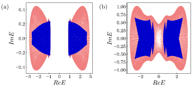
Figure 9: Comparing the continuum band spectrum $E_{c}$ (in blue), defined for the slab geometry in the limit of $L\rightarrow\infty$, with the bulk energy spectrum $E_{\text{bulk}}$ (in red) for model $H_{3}$. (a) For phase C${}_{1}^{\mathrm{LR}}$ with $m=0.9,t_{1}=0.5$. (b) For phase C${}_{1}^{\mathrm{LL}}$ with $m=1.2$, $t_{1}=1.1$. Notice the gap opening as the boundary conditions change in case (b).

The rough contour of the phase boundaries can be obtained from numerical diagonalization of the matrix $\mathcal{T}$ for finite $L$. For example, one can monitor the minimum magnitude of the eigenenergy, $|E|_{\text{min}}$. On the one hand, this quantity is finite for gapped phases (e.g., phase T) that are topologically trivial, i.e., have no edge states, or gapless phases (e.g., phase GL₂) that avoid $E=0$. On the other hand, it vanishes for topological phases with edge modes (e.g., phase C₁ and S^′). Such a quick scan, however, has trouble in locating the precise boundary of phase GL₁ which is gapless and contains $E=0$. In particular, one notices that the numerical spectrum depends sensitively on $L$. It is well-known that diagonalization of large non-Hermitian matrices can experience numerical instabilities, and caution must be exercised before trusting their accuracies, see Refs. Yang et al. (2020); Colbrook et al. (2019); Bergholtz et al. (2021); Böttcher (2005); Reichel and Trefethen (1992) for detailed discussions. Thus, an alternative, algebraic method that works well in the limit of $L\rightarrow\infty$ is desired.

We reiterate the key point that for non-Hermitian Chern insulators, the knowledge of the bulk spectrum may offer little help in determining or understanding its slab phase diagram as we have witnessed in the case of $H_{2}$. For model $H_{3}$ here, the bulk energy $E_{\text{bulk}}(k_{x},k_{y})$ closes its gap along the line of $m=2$ at $k_{x}=k_{y}=0$, and along the line of $t_{1}=1$ at $k_{y}=0$ and $\cos k_{x}=m-1$. While the $m=2$ line agrees with the phase boundary between C${}_{1}^{\mathrm{LR}}$ and T, the $t_{1}$ line, as we shall show below, is not a phase transition line. Moreover, the bulk spectrum fails to predict phase C${}_{1}^{\mathrm{LL}}$, GL₁, and S^′.

Now we show that all the phase boundaries in the limit of $L\rightarrow\infty$ can be worked out from the analytically continued Hamiltonian $\mathcal{H}_{3}(\beta\in\mathrm{GBZ},k_{y})$. For any given value of $k_{y}$, the GBZ can be computed using the two algorithms outlined in Secs. II.C and II.D. As a simple example, let us consider the cutline $m=1$ with varying $t_{1}$, and focus on $k_{y}=0$. In this case, Theorem 9 was already proved back in Eqs. (39) and (40). With the GBZ being a circle, we can parametrize it using a fake wave vector $\tilde{k}_{x}$:

$$\beta=r_{3}e^{i\tilde{k}_{x}}.$$ (91)

Then the continuum band spectrum simplifies for $t_{1}<2$:

$$E^{2}(\tilde{k}_{x},k_{y}=0)=1-\frac{{t_{1}}^{2}}{2}-it_{1}\sqrt{4-t_{1}^{2}}\sin(2\tilde{k}_{x}).$$ (92)

Immediately, we see that for $\tilde{k}_{x}=0$, $E$ vanishes when $t_{1}=\sqrt{2}$, which marks the tricritical point between phases C${}_{1}^{\mathrm{LL}}$, GL₁, and S^′. Away from the central $m=1$ line, an analytical solution seems out of reach, and the GBZ has to be found numerically to yield the continuum bands.

For the purpose of finding the phase boundaries, however, it is not necessary to gain a full knowledge of either the GBZ or the continuum bands. It turns out that for model 3, one only needs to check when the energy gap closes at $E=0$ at some $k_{y}$ values, say $k_{y}=0$. Below, we outline how this problem can be reduced to solving a quartic equation. Following the notation introduced in Sec. II, let $\xi_{i}$ with $i=1,2,3,4$ be the four solutions to the quartic equation

$$\epsilon(\beta)=a\beta^{2}+b/\beta^{2}+c\beta+d/\beta+f=0,$$ (93)

with their magnitudes ordered according to Eq. (41). In other words, $\xi_{i}$ are the preimages of $\epsilon=0$. Then a gap closing, $E(\beta\in\mathrm{GBZ},k_{y}=0)=0$, requires the two roots of the quartic Eq. (93) to have the same amplitude:

$$|\xi_{2}|=|\xi_{3}|.$$ (94)

Recall that the coefficients $a$ to $f$ depend on parameter $m$ and $t_{1}$. Thus, to find points on the $(m,t_{1})$ plane where Eq. (94) is satisfied, we can simply follow a given horizontal or vertical cut and plot $|\xi_{i}|$ to see where $|\xi_{2}|$ and $|\xi_{3}|$ intersect. (While the roots of quartic equations are analytically known, they are unwieldy to manipulate so we opt to find and compare $|\xi_{2}|$ and $|\xi_{3}|$ numerically.) The phase boundaries obtained this way are summarized in Fig. 1(c). They agree with the rough outline from numerical diagonalization of finite-size slabs. The main advantage of the algebraic approach is that the phase boundaries (e.g., that of phase GL₁) can be obtained precisely. Compared to model 2, here the phase boundaries of model 3 are no longer simple analytical curves, but we still find it remarkable that it follows from the solution of a quartic equation.

Once these boundaries are drawn from the gap closing condition, we can investigate the continuum bands in each region. For example, one can confirm that C₁ and T are gapped with a line gap, while GL₁, GL₂, and S^′ are gapless. Figure 9 highlights the contrast between the bulk spectrum (red) and the slab spectrum (blue) in the limit of $L\rightarrow\infty$ obtained from $\mathcal{H}_{3}$. For example, the existence of the line gap (and the edge states) within phase C${}_{1}^{\mathrm{LL}}$ would have been completely missed by only considering $E_{\text{bulk}}(k_{x},k_{y})$. To unambiguously identify each phase, in the next subsection we proceed to look into their edge spectra and topological invariants. For example, we shall see that regions C${}_{1}^{\mathrm{LR}}$ and C${}_{1}^{\mathrm{LL}}$ are divided by a transition line at $t_{1}=1$ where the edge modes change location.

V.2 The dispersion and location of edge modes

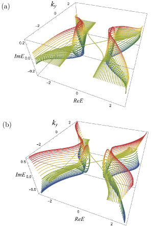
Figure 10: The spectrum of $H_{3}$ in slab geometry (with slab width $L=35$) inside (a) the C${}_{1}^{\mathrm{LR}}$ region for $m=0.9$, $t_{1}=0.5$, and (b) the C${}_{1}^{\mathrm{LL}}$ region with parameters $m=1.2$ and $t_{1}=1.1$. In both cases, a pair of edge modes $E^{\pm}_{\text{edge}}=\pm\sin k_{y}$ transverse the line gap. Note, however, that for case (a), one mode is localized on the right edge and the other on the left edge, whereas in (b), both edge modes are localized on the right edge. The transition in the localization behavior occurs at line $t_{1}=1$ which separates region C${}_{1}^{\mathrm{LR}}$ and C${}_{1}^{\mathrm{LL}}$.

To find the edge states and prove Theorems 12-14 for model $H_{3}$, we once again face the big matrix $\mathcal{T}$ in Eq. (22). But this time its submatrices are given by

$$A = [m-\cos k_{y}]\sigma_{z}+\sin k_{y}\sigma_{y},$$ (95)

$$B = [(-t_{1}-1)\sigma_{z}+i\sigma_{x}]/2,$$ (96)

$$C = [(t_{1}-1)\sigma_{z}-i\sigma_{x}]/2.$$ (97)

The overall strategy is the same as in Sec. IV.B. The wave functions of the edge modes, however, become more cumbersome due to the non-reciprocal hopping $t_{1}$.

First, consider the semi-infinite geometry ($x\geq 0$) with an open boundary at $x=0$, the left edge. To solve the eigenvalue problem $\mathcal{T}\psi=E\psi$, let us write $\psi$ as

$$\psi=(v_{1},v_{2},v_{3},...)^{T},$$ (98)

where $v_{i}$ is a two-component spinor. This leads to

$$Av_{1}+Bv_{2}=Ev_{1},$$ (99)

$$Cv_{n-1}+Av_{n}+Bv_{n+1}=Ev_{n},\;\;\;(n\geq 2).$$ (100)

In the limit $t_{1}=0$, we conclude $v_{1}=(1,i)^{T}/\sqrt{2}$ and $E=\sin k_{y}$, which we take as the guess solution for the general case. From $v_{1}$, all other $v_{n}$ can be found inductively using Eqs. (99) and (100). Exploiting the properties of Pauli matrices, after some algebra we conclude that

$$v_{n}=\lambda_{n}v_{1},$$ (101)

where $\lambda_{n}$ is a number. Within this ansatz, Eqs. (99) and (100) become the following recursion relation for $\lambda_{n}$:

$$(2+t_{1})\lambda_{n}=2(m-\cos k_{y})\lambda_{n-1}+t_{1}\lambda_{n-2},$$ (102)

with the initial condition

$$\lambda_{0}=0,\;\;\lambda_{1}=1.$$ (103)

We seek a solution of the power-law form $\lambda_{n}=\lambda^{n}$. Here $\lambda$ describes the decay (or growth) of the wave function $\{v_{n}=\lambda_{n}v_{1}\}$, and must obey the quadratic equation

$$(2+t_{1})\lambda^{2}-2(m-\cos k_{y})\lambda-t_{1}=0.$$ (104)

This equation has two solutions which we call $\lambda_{\pm}$. The general solution is then the superposition $\lambda_{n}=c_{1}\lambda_{+}^{n}+c_{2}\lambda_{-}^{n}$. The initial condition Eq. (103) fixes the coefficients $c_{1,2}$. The final result is

$$\lambda_{n}=\frac{\lambda_{+}^{n}-\lambda_{-}^{n}}{\lambda_{+}-\lambda_{-}}=\sum_{j=0}^{n-1}\lambda_{+}^{n-1-j}\lambda_{-}^{j}.$$ (105)

It decays with increasing $n$ if and only if $|\lambda_{\pm}|<1$, or equivalently, $|\lambda_{+}\lambda_{-}|<1$. This condition can be further simplified by recalling Vieta’s formula,

$$|\lambda_{+}\lambda_{-}|=\frac{t_{1}}{2+t_{1}}<1$$ (106)

for $t_{1}>0$. Note that this criterion is independent of $m$ or $k_{y}$. It follows that that the edge state with energy $E^{+}_{\text{edge}}=\sin k_{y}$ is always localized on the left edge for $t_{1}>0$. This proves Theorem 12.

The calculation of the other edge mode proceeds similarly. For a semi-infinite system ($x\leq 0$) with an open boundary at $x=0$, let us label the wave function as

$$\psi=(...,u_{3},u_{2},u_{1})^{T}.$$ (107)

With ansatz $E^{-}_{\text{edge}}=-\sin k_{y}$, $u^{T}_{1}=(i,1)/\sqrt{2}$, and $u_{n}=\lambda^{n}u_{1}$, one finds that the decay factor $\lambda$ is determined by

$$(2-t_{1})\lambda^{2}-2(m-\cos k_{y})\lambda+t_{1}=0.$$ (108)

This result can also be obtained from Eq. (104) by symmetry arguments and replacing $t_{1}\rightarrow-t_{1}$. For $t_{1}>0$, the magnitudes of the two solutions satisfy

$$|\lambda_{+}\lambda_{-}|=\frac{t_{1}}{|2-t_{1}|}.$$ (109)

Thus, the $E^{-}$ edge mode is localized on the right edge if $t_{1}<1$, and on the left edge if $t_{1}>1$, proving Theorem 13. The transition occurs at $t_{1}=1$.

It is worthwhile to take a closer look at the $E^{-}$ solution above in the region $t_{1}>1$. At $t_{1}=2$, the matrix $C$ becomes singular with a vanishing determinant and its inverse becomes ill defined. Accordingly, $|\lambda_{+}\lambda_{-}|$ diverges according to Eq. (109). We emphasize that there is nothing physically singular at this point. To get a clearer picture, we must recognize that once $t_{1}$ exceeds 1 and the $E^{-}$ mode is localized on the left edge, it is much more natural to find its wave function by starting from the left boundary, rather than from the right boundary as done in Eq. (107). More explicitly, we repeat the same recipe as prescribed in Eq. (98), but this time with ansatz $E^{-}_{\text{edge}}=-\sin k_{y}$ and $v^{T}_{1}=(i,1)/\sqrt{2}$ instead. The corresponding decay factor now satisfies the equation

$$t_{1}\lambda^{2}-2(m-\cos k_{y})\lambda-(t_{1}-2)=0.$$ (110)

The magnitudes of its two solutions obey

$$|\lambda_{+}\lambda_{-}|=\frac{|t_{1}-2|}{t_{1}}.$$ (111)

Compared to Eqs. (109), here the roles of $t_{1}$ and $(t_{1}-2)$ are switched, now that we seek the edge state wave function starting from the left boundary. It follows that the $E^{-}_{\text{edge}}$ mode is localized on the left edge if $t_{1}>1$, and on the right edge if $t_{1}<1$. This is consistent with our result obtained in the preceding paragraph and provides an alternative proof of Theorem 13. The calculation here also yields the decay factor along the line $t_{1}=2$, where $Cv_{1}=0$. In this case, Eq. (110) reduces to a linear equation, and we have $\lambda=2(m-\cos k_{y})/t_{1}$, and $\lambda_{n}=\lambda^{n}$.

To summarize, within the region C${}_{1}^{\mathrm{LR}}$, the two modes $E^{\pm}_{\text{edge}}$ reside on opposite edges of the slab. In region C${}_{1}^{\mathrm{LL}}$ and phase S^′, they both reside on the left edge, which is impossible for Hermitian Chern insulators. At the transition line $t_{1}=1$, where $|\lambda_{+}\lambda_{-}|=1$, the $E^{-}_{\text{edge}}$ mode permeates into the bulk, and therefore strictly speaking is no longer an “edge mode.” These analytical results agree with the edge states obtained from numerical diagonalization of finite systems, see Fig. 10.

V.3 Chern numbers

For each given value of $k_{y}$, the GBZ curve of $\mathcal{H}_{3}(\beta,k_{y})$ can be found by following the recipes described in Section II. As $k_{y}$ is varied from $-\pi$ to $\pi$, the GBZ curve deforms to produce a 2D surface GBZ_s defined in Eq. (12), which is continuous but may have singularities. Figure 2 shows an example of GBZ_s for $m=0.6$ and $t_{1}=0.4$. Once the GBZ surface is known, one can proceed to compute the Chern numbers using Eq. (87) by discretizing the GBZ_s into patches. One can verify that region C${}_{1}^{\mathrm{LR}}$ and C${}_{1}^{\mathrm{LL}}$ have the same Chern numbers $\pm 1$, while region T is topologically trivial with Chern number zero.

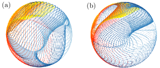
Figure 11: Chern number determined from the eigenvectors of model $H_{3}$ on the Bloch sphere. (a) Region C${}_{1}^{\mathrm{LR}}$ with $m=0.6$, $t_{1}=0.4$. Different colors correspond to a discrete set of $k_{y}$ values from $0$ to $2\pi$, while the data points of the same color depict transversing the GBZ curve for a given $k_{y}$. As $(\beta,k_{y})$ varies throughout the GBZ_s, the eigenvector covers the Bloch sphere exactly once. (b) Region C${}_{1}^{\mathrm{LL}}$ with $m=1.2$, $t_{1}=1.1$. Here, again $k_{y}$ varies from $0$ to $2\pi$ and the eigenvector covers the Bloch sphere exactly once as $(\beta,k_{y})$ transverse the entire GBZ_s. In the trivial phase T (not shown), the eigenvectors do not cover the whole Bloch sphere.

Since the discretization of GBZ_s is numerically involved, we also extract the Chern number by counting the number of times the right eigenvector in Eq. (88) wraps around the Bloch sphere, as done for model 2 in Sec. IV.C. According to Fig. 11, within phase C₁, including region C${}_{1}^{\mathrm{LR}}$ shown in panel (a) and region C${}_{1}^{\mathrm{LL}}$ shown in panel (b), the eigenstate wraps the Bloch sphere once. Within the trivial phase T, the eigenstate does not cover the entire sphere. This verifies that C${}_{1}^{\mathrm{LR}}$ and C${}_{1}^{\mathrm{LL}}$ differ topologically from phase T, and finishes the proof of Theorem 10. We emphasize that Theorem 10 here relies on numerical evaluation of the Chern number and the phase boundary from a well-defined algebraic problem. This is slightly different from the proof of, e.g., Theorem 7, where the phase boundary is simple and analytically known.

V.4 The gapless phase S^′

A large area of the phase diagram Fig. 1(c) is occupied by the gapless phase S^′. An example of the slab spectrum within this phase is shown in Fig. 12 for $t_{1}=1.9$ and $m=1$. One observes that the two bands merge into a single membrane in the space of $(k_{y},\mathrm{Re}E,\mathrm{Im}E)$. While the spectrum on the complex energy plane appears gapless, the membrane possesses a hole around $E=0$, which becomes apparent when projected on the $(k_{y},\mathrm{Im}E)$ plane. In other words, within a certain interval of $k_{y}$ values around $k_{y}=0$, the spectrum is gapped. This situation is very different from Dirac semimetals, where the gap closes at isolated point degeneracies. A pair of edge modes $E^{\pm}_{\text{edge}}=\pm\sin k_{y}$ transverse the hole, and both of them reside on the left edge as proved in Sec. V.B. Note the edge states here differ from those in phase S of model $H_{2}$ which cross $E=0$ at $k_{y}=\pi$ instead, see Fig. 8. We have checked that the edge states are robust against on-site disorder, e.g., in the value of $m$.

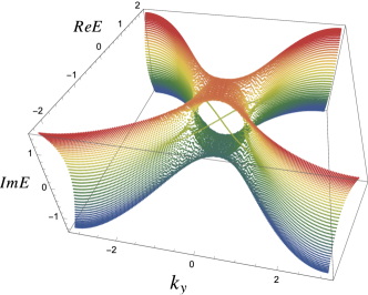
Figure 12: The spectrum of $H_{3}$ in slab geometry inside the gapless phase S^′, $m=1$, $t_{1}=1.9$, $L=50$. The continuum bands form a single surface/membrane. Two edge modes transverse the hole of the membrane, crossing $E=0$ at $k_{y}=0$. Both of them are localized on the left edge.

In short, this gapless phase is a rather unique feature of non-Hermitian Chern insulators. The edge states are separated from the continuum bands in the imaginary part of the energy, and therefore in principle can be probed by dynamics Hu et al. (2022). In some sense, the existence of phase S^′ attests to the resilience of non-Hermitian Chern insulators. When the gap is forced to close, for example, by increasing the non-reciprocal hopping parameter $t_{1}$ at fixed $m$, the edge modes may survive. The persistence is most apparent along the line of $m=1$ in the phase diagram Fig. 1(c).

VI Comparison to earlier work and outlook

A large body of work has been devoted to study non-Hermitian tight-binding models. For a more comprehensive review of recent progress in this field, see, for example, Refs. Ashida et al. (2020); Bergholtz et al. (2021); Okuma and Sato (2022); Ghatak and Das (2019). Here we only mention a few works that provided crucial techniques used in our paper or set the stage for our work. Non-Hermitian Hamiltonians describing particles hopping in 1D, such as the Hatano-Nelson model Hatano and Nelson (1996); Gong et al. (2018), the generalized Su-Schrieffer-Heeger Su et al. (1979); Lieu (2018); Yao and Wang (2018); Kunst et al. (2018); Lee (2016), and Rice-Mele model Rice and Mele (1982); Wang et al. (2018); Zhang et al. (2019); Yi and Yang (2020) are well understood. These models showcase a number of phenomena including the non-Hermitian skin effect and exceptional points in the energy spectrum that are unique to non-Hermitian systems. To characterize the topology of these non-Hermitian systems, unique concepts and techniques were developed, beyond the established framework for Hermitian Bloch Hamiltonians. The initial theoretical efforts focused on the classification of the topological phases based on the dichotomy between point gaps and line gaps Gong et al. (2018); Kawabata et al. (2019a, b); Zhou and Lee (2019); Liu and Chen (2019); Liu et al. (2019). Later works gave a more general classification using braid groups Wojcik et al. (2020); Li and Mong (2021) and knots Hu and Zhao (2021) for non-Hermitian models with separable bands Shen et al. (2018). For multiband systems in 1D with an odd number of bands, invariants can be constructed through the Majorana stellar representation Bartlett et al. (2021); Teo et al. (2020); Xu et al. (2020). To restore the bulk boundary correspondence, the notion of GBZ was introduced in Yao and Wang (2018) and Yokomizo and Murakami (2019) for 1D non-Hermitian Hamiltonians. And the topological origin of the non-Hermitian skin effect in 1D was clarified in Refs. Zhang et al. (2020); Okuma et al. (2020); Gong et al. (2018); Borgnia et al. (2020); Zhang et al. (2020); Okuma et al. (2020); Longhi (2019); Jiang et al. (2019) and attributed to the existence of point gap, which allows the winding number to be defined as the topological invariant. Compared to the thorough understanding achieved in 1D, non-Hermitian topological phases in 2D and 3D are much less understood with many questions remaining open.

Now we compare our approach and results to a few existing works on non-Hermitian Chern insulators in 2D. In Ref. Yao et al. (2018), Yao et al. considered a generalized Qi-Wu-Zhang model with imaginary magnetic fields. They compared the bulk phase diagram (Fig. 1 in Ref. Yao et al. (2018)) with that of the slab phase diagram (Fig. 3 in Ref. Yao et al. (2018)) obtained by defining a non-Bloch Chern number. These authors treated the non-Hermitian term as a small perturbation, and computed the Chern number using a continuum approximation. In our work, no approximation or extrapolation of the Hamiltonian was made, and the procedure used to compute the GBZ_s and continuum bands are general. We stress that our strategy of computing the GBZ_s of 2D models builds on the original algorithm outlined in Yokomizo and Murakami (2019), the notion of auxiliary GBZ curves Yang et al. (2020), and the self-intersection method Wu et al. (2022).

Model $H_{2}$ in our work was introduced by Kawabata et al. Kawabata et al. (2018). These authors obtained the slab phase diagram (Fig. 7 in Ref. Kawabata et al. (2018)) numerically and compared to the bulk phase diagram (Fig. 1 in Ref. Kawabata et al. (2018)). They also analytically derived the dispersion of the edge modes, and found their localization in the slab geometry (roughly speaking the content of Theorems 3 and 4 here). Here, we take several steps further to obtain the GBZ, the continuum bands, the Chern numbers, and the analytical forms of all the phase boundaries. We also give a precise identification of the gapless phase S and phase C₂ in terms of their continuum band structure and Chern numbers. Our phase diagram Fig. 1(b) labels the phases differently from Kawabata et al. (2018). These new results, summarized in Theorems 1 and 2 and 5-8, give a thorough understanding of this non-Hermitian Chern insulator.

Other theoretical approaches have been proposed to describe non-Hermitian topological phases in 2D. References Kunst and Dwivedi (2019) introduced a framework based on the transfer matrix in real space to analyze the Qi-Wu-Zhang model with imaginary fields, and Ref. Borgnia et al. (2020) employed single and doubled Green’s functions to describe the Qi-Wu-Zhang model in an imaginary magnetic field, including the boundary modes and the phase diagram. Reference Chang et al. (2020) employed the entanglement spectrum to determine topological properties in the gapped phases of the Qi-Wu-Zhang model in an imaginary magnetic field along the $y$ direction. Reference Song et al. (2019) constructed real-space topological invariants to characterize the topological phases for the Qi-Wu-Zhang model in an imaginary magnetic field. Reference Wang et al. (2020) characterized a non-Hermitian Qi-Wu-Zhang model obtained by a similarity transformation, and proposed a topological invariant for classification. In passing, we also mention Ref. Leykam et al. (2017) which focused on non-Hermitian Dirac Hamiltonians with gapless spectrum and exceptional points. Reference Franca et al. (2022) proposed an alternative avenue toward realizing non-Hermitian 2D models using waves backscattered from the boundaries of insulators. A geometric visualization of the topology of non-Hermitian 2D modes based on the $\mathbf{d}$ vector was advocated in Ref. Li et al. (2019). We borrow this perspective in our treatment of model $H_{1}$. Note, however, the 2D model studied in Eqs. (31) and (32) of Ref. Li et al. (2019) was more complicated than $H_{1,2,3}$ here. A more general version of $H_{3}$ was mentioned in Ref. Zhang et al. (2022) in discussing the non-Hermitian skin effect.

The main objective of this paper is to outline an algebraic procedure to reliably predict the fascinating slab phase diagrams, including the behaviors of edge modes, for non-Hermitian Chern insulators. The algebraic procedure does not rely on numerical diagonalization of finite size systems, and therefore is free from the numerical errors that plague the diagonalization of large non-Hermitian matrices. This is not a trivial task, for we have seen GBZ_s with cusps and singularities, topological gapless phases such as S and S^′ or the higher Chern number phase C₂ that are unexpected from bulk analysis, and edge states switching sides while the Chern numbers remain the same. The breakdown and resurrection of the bulk-edge correspondence is illustrated by two examples, $H_{2}$ and $H_{3}$. Such refinement in the understanding of generalized Qi-Wu-Zhang model is achieved by combining various bits of technology available in the literature: analytical continuation, calculation of GBZ curves, analytical solution of the edge spectrum, visualization of the Chern number etc. We hope these examples are helpful to readers who are interested in analyzing other non-Hermitian topological phases of matter in 2D and 3D.

We have focused exclusively on the slab geometry to limit the paper to a reasonable length. An open question is to analyze the edge and corner modes in finite systems with open boundaries in both the $x$ and $y$ directions, e.g., a rectangle of size $L_{x}\times L_{y}$. As pointed out in Ref. Hu et al. (2022), the edge states of a non-Hermitian Chern insulator may gravitate to corners due to the skin effect, forming the so-called boundary-skin mode. The 1D theory established in Refs. Zhang et al. (2020); Okuma et al. (2020) can be applied to the effective Hamiltonian that describes the edge degrees of freedom in the slab geometry to understand their corner localization in rectangle geometry. Our preliminary analysis indicates that this scenario is possible for both model $H_{2}$ and model $H_{3}$. A comprehensive analysis of the non-Hermitian skin effect in 2D Chern insulators is beyond the scope of this paper and left for future work.

Non-Hermitian lattice models have been realized in experiments using topological electric circuits Lee et al. (2018); Stegmaier et al. (2021); Liu et al. (2020), coupled optical ring resonators Longhi et al. (2015); Wang et al. (2021a, b), nitrogen-vacancy centers Wu et al. (2019); Liu et al. (2021); Zhang et al. (2021); Yu et al. (2022), cavity opto-mechanical systems Patil et al. (2022), phononic crystals with active acoustic components Liu et al. (2022), and mechanic metamaterials Ghatak et al. (2020) to name just a few. These experimental techniques can potentially be applied to realize the models described here. Once their topological properties are characterized and understood, non-Hermitian systems may offer exciting opportunities for applications such as topological lasing Peng et al. (2014); Brandstetter et al. (2014); Harari et al. (2018); Bandres et al. (2018); Parto et al. (2018); Zhao et al. (2018); Ota et al. (2020); Comaron et al. (2020); Sone et al. (2020); Zapletal et al. (2020); Kim et al. (2020); Wong and Oh (2021); Zhu et al. (2021); Ezawa (2022), enhanced quantum sensing Budich and Bergholtz (2020); Bao et al. (2021); Wang et al. (2022), and quantum batteries Konar et al. (2022).