Level occupation switching with density functional theory

Abstract

The charge transport properties of zero-temperature multi-orbital quantum dot systems with one dot coupled to leads and the other dots coupled only capacitatively are studied within density functional theory. It is shown that the setup is equivalent to an effective single impurity Anderson model. This allows to understand the level occupation switching effect as transitions between ground states of different integer occupations in the uncoupled dots. Level occupation switching is very sensitive to small energy differences and therefore also to the details of the parametrized exchange-correlation functionals. An existing functional already captures the effect on a qualitative level but we also provide an improved parametrization which is very accurate when compared to reference numerical renormalization group results.

I Introduction

Quantum dots (QDs) are an ideal testbed to investigate the interplay between quantum many-body physics and transport phenomena. They can be fabricated in the lab from a large variety of materials and techniques, such as metallic nanoparticles[1], lateral confinement of a two-dimensional electron gas (2DEG) in GaAs/AlGaAs heterostructures (for a review see Ref. 2 and references therein), carbon nanotubes (CNTs)[3, 4], and molecular junctions[5]. Indeed important many-body phenomena such as the Kondo effect[6] and Coulomb blockade (CB)[7], characteristic for so-called strongly correlated electrons, where electronic interactions dominate over the kinetic energy, have been measured in transport setups of QDs.[8, 9, 5, 10, 11]

The physics of QDs can be further enriched by the existence of multiple electronic levels (or orbitals), or by coupling of QDs. The interplay between strong electronic correlations and the spin and orbital degrees of freedom in multi-orbital QDs, may lead to new physical phenomena, such as the SU(4) and underscreened Kondo effects, which have both been measured in CNTs.[12, 13, 14] An interesting effect may occur in multi-orbital QDs when one of the QD levels couples more strongly to the leads than the other levels. In this case abrupt changes in the conductance and transmission phases between Coulomb blockade peaks have been observed.[15, 16, 17, 18, 19, 20] These may be attributed to the so-called level occupation switching (LOS), where the strongly coupled level is abruptly emptied, while the weakly coupled level(s) are abruptly filled, or vice versa. [21, 22, 23, 24, 25, 26] In essence this phenomenon is a result of the competition between the kinetic energy of the strongly coupled level and its electrostatic repulsion with the weakly coupled levels.[23]

Density functional theory (DFT) is one of the most successful and popular approaches for computing the electronic structure of molecules and solids owing to its relative simplicity and computational efficiency.[27, 28, 29] Since DFT is in principle an exact (many-body) theory for the ground-state energy and density of a many-electron system, it should also be capable of describing strong electronic correlation phenomena such as Kondo effect, Coulomb blockade, and ultimately the LOS effect. However, in practice approximations need to be made in DFT for the exchange-correlation (xc) part of the total energy functional. And unfortunately, the most popular approximations to DFT, such as the local-density[28] and generalized-gradient approximations[30, 31, 32] in condensed-matter physics, and the so-called hybrid functionals in chemistry,[33] are known to fail for strongly correlated systems.

Nevertheless, if equipped with proper approximations for the xc part of the functional, DFT is indeed capable of describing strongly correlated phenomena such as Coulomb blockade and Kondo effect in transport through nanoscale devices,[34, 35, 36] and the Mott-Hubbard gap in solids.[37] More recently, it has also been shown that the actual many-body spectral function may be extracted from a DFT calculation by making use of an extension of DFT called i-DFT.[38, 39] This DFT framework also allows to describe the Mott metal-insulator transition, one of the hallmarks of strong electronic correlations.[40] The crucial ingredient for the description of these phenomena within DFT are steps at integer occupations in the xc potentials.[41] These steps are related to the famous derivative discontinuity of exact DFT [42], which is missing in the standard approximations. In the context of the Anderson impurity model, the step feature in the xc potential gives rise to the pinning of the Kohn-Sham (KS) impurity level to the Fermi energy, which results in a plateau for the zero-bias conductance as a function of the applied gate, in accordance with the Kondo effect.[29, 30, 31]

Here we show how DFT can be used to study the LOS phenomenon which occurs in multi-level quantum dot (MQD) systems in the asymmetric situation where only one of the levels is connected to leads. In Section II we introduce the model and show how it can exactly be mapped onto an effective single impurity Anderson model (SIAM). In Section III we use lattice DFT for the effective SIAM and an energy minimization argument to decide which configuration of integer occupations of the disconnected dots is realized. In Section IV we show that an existing parametrization of the SIAM Hxc potential already qualitatively captures the LOS effect although not always at the correct value of the gate. The origin of these deviations is investigated and remedied by a re-parametrization of the Hxc functional. Finally, we present our conclusions in Section V.

II Model

We consider a multi-orbital quantum dot consisting of $M$ impurities which can hold up to two electrons and which are all capacitively coupled among each other. We consider the situation when only one of the impurities is connected to two leads and we also restrict ourselves to the zero-temperature limit. The total Hamiltonian of the system is given as the sum of the Hamiltonians of the isolated dot and leads, as well as the coupling between them and reads

$$\hat{H}=\hat{H}_{{\rm MQD}}+\sum_{\alpha k\sigma}\varepsilon_{\alpha k}\hat{c}^{\dagger}_{\alpha k\sigma}\hat{c}_{\alpha k\sigma}$$

$$+\sum_{\alpha k\sigma}\left(t_{\alpha k}\hat{d}^{\dagger}_{1\sigma}\hat{c}_{\alpha k\sigma}+{\rm H.c.}\right)$$ (1)

where

$$\hat{H}_{{\rm MQD}}=\sum_{i=1}^{M}v_{i}\hat{n}_{i}+\sum_{i=1}^{M}U_{i}\hat{n}_{i\uparrow}\hat{n}_{i\downarrow}+\sum_{i<j}^{M}U_{ij}\hat{n}_{i}\hat{n}_{j}$$ (2)

describes the capacitatively coupled MQD where $\hat{n}_{i}=\hat{n}_{i\uparrow}+\hat{n}_{i\downarrow}$ is the number operator for level $i$ with $\hat{n}_{i\sigma}=\hat{d}_{i\sigma}^{\dagger}\hat{d}_{i\sigma}$ and $\hat{d}_{i\sigma}$ ($\hat{d}_{i\sigma}^{\dagger}$) are the annihilation (creation) operators for electrons with spin $\sigma$ in orbital $i$. In Eq. 2, $v_{i}$ and $U_{i}$ are the on-site energy (also referred to as gate) and the intra-Coulomb repulsion of level $i$ while $U_{ij}$ is the inter-Coulomb repulsion between levels $i$ and $j$. The second term in Section II describes the non-interacting electrons in left (L) and right (R) leads ($\alpha=L,R$) while the third term accounts for the (symmetric) coupling of the first impurity to left and right leads. The resulting broadening functions $\Gamma_{\alpha}({\omega})=2\pi\sum_{k}|t_{\alpha k}|^{2}\delta({\omega}-\varepsilon_{\alpha k})$ are assumed to describe featureless leads and therefore become independent of frequency, i.e., we take the wide band limit (WBL) with $\Gamma_{\alpha}({\omega})=\gamma_{\alpha}$. In Fig. 1 a schematic representation of the MQD setup is shown.

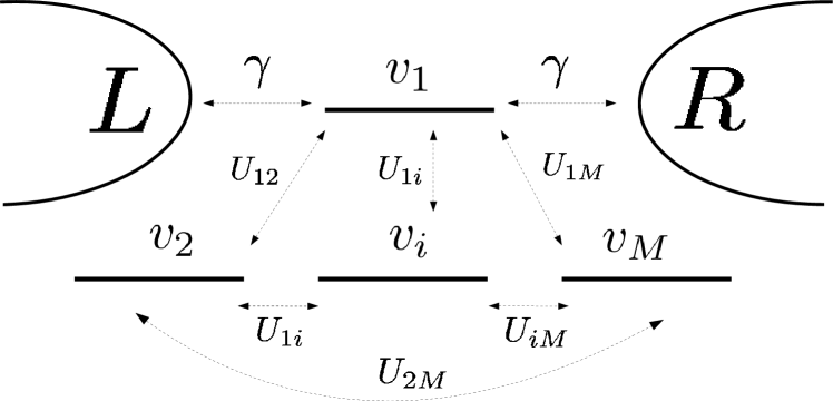
Figure 1: Schematic representation of the transport setup for the MQD. The first impurity is connected to the electron reservoirs while the rest only interact through electrostatic repulsions with each other.

Since the impurities $j=2,\ldots,M$ are not connected to the reservoirs, the multi-orbital quantum dot system can be mapped exactly onto an effective SIAM.[23] This follows from the fact that the operators $\hat{n}_{j\sigma}$ for $j>1$ all commute with the Hamiltonian of Section II. Therefore, all the many-body eigenstates of $\hat{H}$ can be chosen to be eigenstates of $\hat{n}_{j\sigma}$ (for $j>1$) and the corresponding eigenvalues take values $n_{j\sigma}=0,1$. Therefore, the total occupations $n_{j}$ of the disconnected dots can only take the integer values $n_{j}=0,1,2$. As a consequence of this commutation property, when the Hamiltonian is applied to an eigenstate of $\hat{n}_{j\sigma}$ ($j>1$), the problem is seen to be equivalent to an effective SIAM related to the first impurity with an effective potential

$$v_{1}^{\rm eff}=v_{1}+\sum_{j=2}^{M}U_{1j}n_{j}$$ (3)

and an additional constant contribution to the total energy given by $\sum_{j\neq 1}U_{j}\delta_{n_{j},2}$. Therefore, the only effect of charging and discharging the levels $j=2,\ldots,M$ is to modify the average Hartree potential felt by the first level.

III Lattice density functional theory

With the observations of the previous Section it is clear that any many-body method which can accurately treat the SIAM can be employed to obtain the ground state energy and density of $\hat{H}$. Here our method of choice is lattice DFT which in the past has successfully been used for the SIAM. [34, 35, 36, 43].

III.1 Energy functional

In lattice DFT, for a given set of gates $\mathbf{v}=(v_{1},\ldots,v_{M})$ the total energy functional for the interacting system described by $\hat{H}$ reads

$$E[\mathbf{n}]=T_{s}[n_{1}]+E_{\rm Hxc}[\mathbf{n}]+\sum_{i=1}^{M}n_{i}v_{i},$$ (4)

where $T_{s}[n_{1}]$ is the non-interacting kinetic energy of the only impurity connected to leads (the kinetic energy of the disconnected dots vanishes). $E_{\rm Hxc}[\mathbf{n}]$ is the Hartree-exchange-correlation (Hxc) energy which is a functional of all densities and we used the notation $\mathbf{n}=(n_{1},\ldots,n_{M})$. The non-interacting kinetic energy can be expressed in terms of the (local) Green function $G^{R}_{d}(\omega)$ of the connected dot as $T_{s}=\frac{\gamma}{\pi}\int_{-\varepsilon_{C}}^{0}d\omega\text{Re}\left[G_{d}^{R}(\omega)\right]$. Here $\varepsilon_{C}$ is an energy cutoff which ensures the convergence of the integral. In the WBL the non-interacting kinetic energy contribution can be expressed in a closed form (see Appendix for the detailed derivation) as

$$T_{s}[n]=\frac{\gamma}{2\pi}\log\left[\frac{\frac{\gamma^{2}}{4}\left(\tan{\left(\frac{\pi}{2}(1-n)\right)}^{2}+1\right)}{\varepsilon_{C}^{2}+\frac{\gamma^{2}}{4}}\right].$$ (5)

Note that the energy cutoff only acts as a constant shift to the total energy but does not change its shape. Therefore both the energy minimum and any energy difference between different configurations are independent of the value of $\varepsilon_{C}$.

The Hxc energy functional $E_{\rm Hxc}[\mathbf{n}]$ of the total system can be simplified using the considerations of the previous Section. Since for the disconnected dots $i\in\{2,\ldots,M\}$, the only possible occupations are $n_{i}=0,1,2$ (and the KS system has to reproduce these occupations), $E_{\rm Hxc}$ may be written as

$$E_{\rm Hxc}[\mathbf{n}]=E_{\rm Hxc}^{\rm SIAM}[n_{1}]+\sum_{i<j}^{M}U_{ij}n_{i}n_{j}+\sum_{j=2}^{M}U_{j}\delta_{n_{j},2}$$ (6)

where $E_{\rm Hxc}^{\rm SIAM}[n]$ is the Hxc functional for a simple SIAM. Inserting Eq. 6 into Eq. 4 it becomes immediately clear that the resulting total energy functional has the form of the energy of a single Anderson impurity but with effective on-site potential $v_{1}^{\rm eff}$ given by Eq. 3.

For a given set of gate levels ($v_{1},\ldots,v_{M}$), there are $3^{M-1}$ different configurations of occupations ($n_{2},\ldots,n_{M}$) of the disconnected dots. The ground state energy and the resulting set of occupancies of the system can then be obtained by comparing the energies of the different configurations of available states and taking the one corresponding to the minimum of energy. In the degenerate case $v_{i}=v$, the ground state energy of the system can be found by minimizing the universal functional $F[n]=T_{s}[n]+E_{Hxc}[n]$, since the last term of Eq. 4 is constant (at given fixed total occupation) due to the one-to-one correspondence between total occupation $N$ and the external potential $v$.

A LOS event exactly corresponds to a change in the ground state energy of the system, and provided an accurate parametrization for the SIAM Hxc energy $E_{\rm Hxc}^{\rm SIAM}$ is used, this event can be completely captured within DFT.

III.2 Kohn-Sham equation

For a given configuration of (integer) occupations ($n_{2},\ldots,n_{M}$) of the disconnected dots, the (non-integer) density on the connected dot can now be found by the Hohenberg-Kohn variational principle, i.e., by searching for the value $n_{1}$ which minimizes the total energy (4). Therefore we need to solve $\frac{\partial E[\mathbf{n}]}{\partial n_{1}}=0$ which is easily shown to be equivalent to solving the KS equation

$$n_{1}=1-\frac{2}{\pi}\arctan{\left(2\frac{v_{1}^{\rm eff}+v_{\rm Hxc}^{\rm SIAM}[n_{1}]}{\gamma_{1}}\right)},$$ (7)

where we have used the definition (3) of the effective potential $v_{1}^{\rm eff}$ and defined the SIAM Hxc potential as

$$v_{\rm Hxc}^{\rm SIAM}[n]=\frac{{\rm d}E_{\rm Hxc}^{\rm SIAM}[n]}{{\rm d}n}\;.$$ (8)

We note in passing that Eq. 7 is equivalent to expressing the density as[44]

$$n_{1}=2\int_{-\infty}^{0}\frac{{\rm d}{\omega}}{2\pi}\;A_{s,1}({\omega})$$ (9)

where, without loss of generality, we assumed a vanishing equilibrium chemical potential in the leads. The KS spectral function for the connected dot is

$$A_{s,1}(\omega)=\frac{{\gamma}_{1}}{\frac{{\gamma}_{1}^{2}}{4}+(\omega-v_{s,1})^{2}}\;,$$ (10)

consistent with WBL approximation used to derive Eq. 5, and $v_{s,1}=v_{1}^{\rm eff}+v_{\rm Hxc}^{\rm SIAM}$.

According to Friedel sum rule, in the zero-temperature limit, the impurity spectral function at the Fermi energy is completely determined by the impurity density. Since in the setup considered here only one impurity level is connected to the leads, the zero-bias conductance is directly given by the spectral function at the Fermi level. In this case the Friedel sum rule implies that the electrical conductance of the system is fully determined by the equilibrium density at the impurity and reads[46, 47, 48]

$$G=\sin{\left(\frac{\pi n_{1}}{2}\right)}^{2}.$$ (11)

On the other hand, the correct description of the electrical conductance requires the access to the actual (many-body) electrical current of the system, and therefore one possibility is the inclusion of the xc corrections to the bias of the system. [49, 50, 51] However, since here the exact zero-bias conductance can be expressed explicitly in terms of the ground state density alone (which is a quantity accessible to standard ground state DFT), already the KS zero-bias conductance $G_{s}$ is exact [34, 35, 36, 52, 53] and can be expressed as

$$G=G_{s}=\frac{\frac{\gamma^{2}}{4}}{v_{s,1}^{2}+\frac{\gamma^{2}}{4}}.$$ (12)

Eqs.(11) and (12) provide two equivalent expressions in the zero temperature regime for the zero-bias conductance. [46, 47, 48]

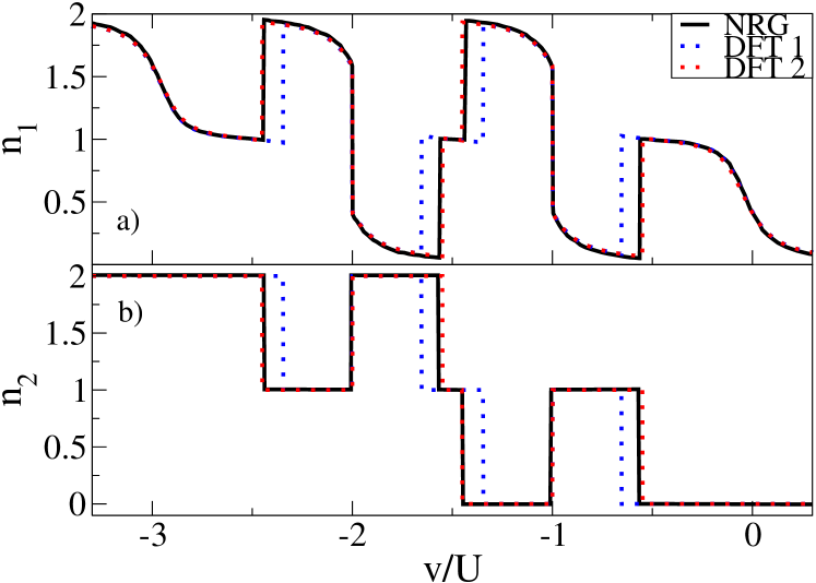
Figure 2: Comparison of the local occupancies obtained with the exchange-correlation functional of Ref. 35 (DFT 1), and those obtained with the new parametrization of Eq. 13 (DFT 2) to the NRG results of Ref. 22. Both $n_{i}$ are shown as function of the gate level for the degenerate case $v=v_{1}=v_{2}$ and for strong correlations $\gamma/U=0.1$.

IV Results

As discussed in Section II, the problem of the capacitively coupled MQD with only one impurity coupled to leads can exactly be mapped onto a SIAM. In the context of lattice DFT (Sec. III) this implies that the only quantity to be approximated is the Hxc functional $E_{\rm Hxc}^{\rm SIAM}$ from which $v_{\rm Hxc}^{\rm SIAM}$ follows by differentiation. Once such a parametrization is given, the MQD DFT problem is solved as follows: For a given set of gate potentials $\mathbf{v}$, for each configuration of (integer) occupations of the disconnected impurities (covering the $3^{M-1}$ possible configurations) we solve the KS equation (7) for $n_{1}$ with the effective potential of Eq. 3 and calculate the corresponding total energies. The lowest of these energies then corresponds to the configuration of the ground state.

For the SIAM functional, we start by considering the new parametrization at zero temperature suggested in Ref. 35. In Fig. 2 we present the local occupancies for the case of the double quantum dot $M=2$ as a function of the gate level in the degenerate case $v=v_{1}=v_{2}$ and strong correlations $\gamma/U=0.1$. The results labeled DFT 1 correspond to the self-consistent densities obtained with the parametrization of Ref. 35. The first thing to note is that our approach does capture the LOS transitions and gives densities which qualitatively agree with the reference NRG results of Ref. 22. However, we also notice that the LOS events take place at values of $v$ considerably different from the many-body results. Since, as mentioned above, the only possible source of error in our approach is the parametrization of $E_{\rm Hxc}^{\rm SIAM}$, below we propose a reparametrization of the functional (DFT 2 in Fig. 2) which correctly and accurately captures the LOS transitions.

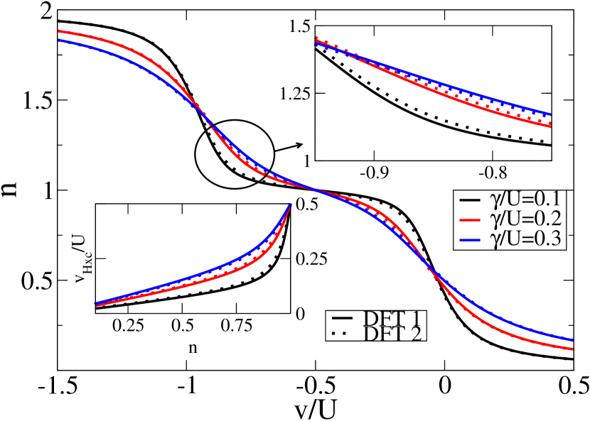
Figure 3: Self-consistent densities of the simple SIAM obtained with the parametrization of $v_{\rm Hxc}^{\rm SIAM}$ given in Ref. 35 (DFT 1) and our new parametrization (DFT 2) as function of gate for different values of $\gamma/U$. The upper insets highlights small differences in the mixed-valence regime while the lower inset shows the Hxc potentials for the two parametrizations.

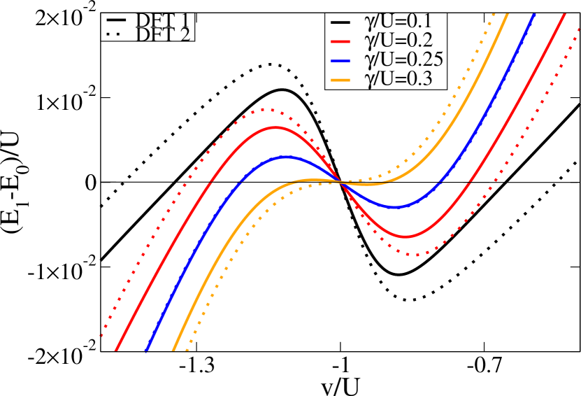
Figure 4: Energy difference between the states with $n_{2}=0$ and $n_{2}=1$ of the double quantum dot for different coupling strengths in the case $v=v_{1}=v_{2}$. The LOS events exactly correspond to the degeneracy of the states $E_{n_{2}=1}=E_{n_{2}=0}$. Note how the new parametrization shifts the crossings of zero of the energy differences, i.e., the gate values at which the LOS event occurs.

The parametrization of Ref. 35 depends on two parameters which are both functions of $\gamma/U$. In order to correctly capture the LOS events we here propose to keep the same functional form but reparametrize the parameter $\sigma$ of Eq. (16) of Ref. 35. Our fit to those numerical values of $\sigma$ which best reproduces the positions of the LOS events for the parameters of Ref. 22 is given as

$$\sigma=0.07\arctan\left(\frac{171.358(\gamma/U)^{2}}{2+\gamma/U}\right)\;.$$ (13)

This newly parametrized Hxc functional for the SIAM will be denoted as DFT 2 in the following. It now accurately captures the gate positions of the LOS events, see Fig. 2.

The gate positions of the LOS events are highly sensitive to the parametrization of the Hxc functional, especially in the mixed valence regime. This can be appreciated in Fig. 3, where we show the self-consistent SIAM densities produced with the DFT 1 (solid line) and the DFT 2 (dashed line) functionals for different coupling strengths. The discrepancies between the corresponding densities are almost negligible, with the maximum disagreement in the mixed valence regime, i.e., in the transition from empty to half occupation and from half occupation to full occupation. In the inset of Fig. 3, both parametrizations of $v_{\rm Hxc}^{\rm SIAM}[n]$ are compared. Note that although the corrections are very small (of the order of $\sim 10^{-3}U$), they are crucial in order to accurately capture the LOS events.

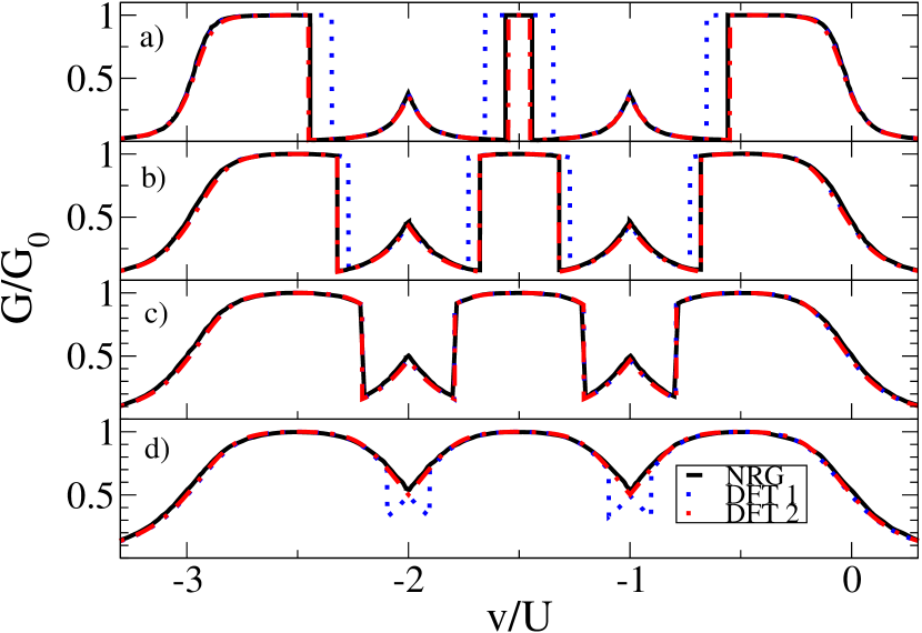
Figure 5: Comparison of the zero-bias conductance obtained with the exchange-correlation functional of Ref. 35 (DFT 1) with the new parametrization (DFT 2) and NRG calculations. $G$ is shown as function of the gate level in the degenerate case $v=v_{1}=v_{2}$ and for different coupling strengths $\gamma/U=0.1,0.2,0.25,0.3$ from a) to d), respectively. All energies in units of U.

In Fig. 4, we show as an illustrative example the difference between the computed energies for two different (integer) $n_{2}$, $E_{n_{2}=1}$ and $E_{n_{2}=0}$, obtained self-consistently with the different parametrizations. The effect of the new parametrization is considerably larger for some values of the coupling strength ($\gamma/U=0.1,0.2,0.3$), while for others it is not appreciable ($\gamma/U=0.25$). In particular, this difference is relevant at $E_{n_{2}=1}-E_{n_{2}=0}=0$, which exactly corresponds to the gate at which the the LOS event occurs. Although not shown in the present paper, the new parametrization does not introduce any change in the $E_{n_{2}=2}=E_{n_{2}=0}$ crossing (only found at $v/U=-1,-2$) while the transition from $E_{n_{2}=2}$ to $E_{n_{2}=1}$ follows exactly the same correction as the one illustrated for gates centered at $v/U=-2$.

IV.1 Results for the double quantum dot

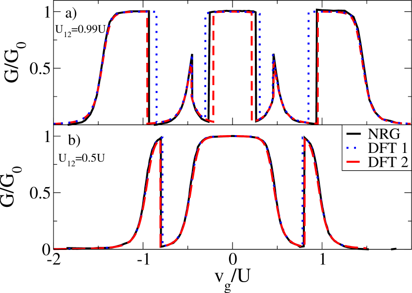
Figure 6: Zero-bias conductance as function of the gate voltage $v_{g}=v-U_{12}-U/2$ in units of $U$ for a) $U_{12}=0.99U$ and b) $U_{12}=0.5U$. In both panels $\gamma/U=0.1$.

In Fig. 5 we present the conductance as function of the gate level in the degenerate case $v=v_{1}=v_{2}$ for different coupling strengths $\gamma/U=0.1,0.2,0.25,0.3$ from a) to d), respectively. For small coupling strength, six LOS events occur, two of them pinned at the gate values $v/U=-2,-1$, related to two peaks usually referred to as CB peaks,[54] since similar structures are present in the CB regime. The other four LOS transitions lead to a widening of the three Kondo plateaus. We observe that the DFT 1 results are qualitatively correct, while still failing to predict the evolution of the LOS events with increasing coupling strength, except for the ones related to the two CB peaks. On the other hand, the DFT 2 results accurately reproduce the NRG calculations, showing the correct evolution of the three Kondo plateaus to wider structures and the two CB peaks into dips for higher values of $\gamma/U=0.3$.

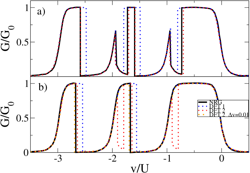
Figure 7: Conductance as function of the gate level in units of $U$ for a) $\Delta v=0.005$ and b) $\Delta v=0.0075$. In both panels $\gamma/U=0.1$.

The results shown so far are related to the fully degenerate case, i.e, $v=v_{1}=v_{2}$ and $U=U_{1}=U_{2}=U_{12}$, but our DFT study can go further. Since the dependence on the inter-Coulomb repulsions only enters into the effective potential felt by the first impurity, we can easily investigate the effects of changing it. In Fig. 6 we show the conductances for a) $U_{12}=0.99U$ and b) $U_{12}=0.5U$ as function of the gate voltage $v_{g}=v-U_{12}-U/2$ in units of $U$. Again, we find that DFT 2 gives an excellent agreement with NRG except for the central plateau in panel a), where the NRG calculations predict a slightly wider central structure. When the inter-Coulomb repulsion is decreased to be half of the intra-Coulomb repulsion, the two CB peaks and the central Kondo plateau merge into a smooth plateau leading to the disappearance of four of the LOS events. On the other hand, in Fig. 7 we explore the effect of considering a finite difference between the gate levels $\Delta v=v_{1}-v_{2}$. In Fig. 7 a) the DFT 2 parametrization correctly captures the evolution of the two CB peaks for $\Delta v=0.005$, while for $\Delta v=0.0075$ (Fig. 7 b)) the DFT 2 results present a finite difference with the reference NRG results. The origin of this discrepancy is not completely clear: it could either be due to subtle details of the Hxc potentials which our parametrization does not capture. However, it could also be due to small numerical effects due to the sensitivity of the LOS events to small energy differences. However, we do find that our results for $\Delta v=0.01$ completely agree with the NRG ones for $\Delta v=0.0075$.

IV.2 Results for more than two dots

We further apply our new parametrization of $v_{\rm Hxc}^{\rm SIAM}$ to the situation of more than two orbitals with only one of them being connected to leads. The generalization is straightforward and only requires to find the ground state energy between the different $3^{M-1}$ states corresponding to the different configurations of integer occupancies of the disconnected dots.

Some results for the fully degenerate case of the triple quantum dot ($v=v_{1}=v_{2}=v_{3}$) for $\gamma/U=0.2$ are presented in Fig. 8. In panel a) the densities predict a total of twelve LOS events. Since both the second and third impurity levels are completely degenerate, a swap in their local occupancies leaves the problem invariant and the corresponding many-body eigenstates are degenerate. Therefore, the (average) occupancies may take semi-integer values for some values of the gate. Following the same reasoning we observe that for the fully degenerate MQD, the $M-1$ degenerate levels of disconnected dots can only reach occupancies of integer multiples of $(M-1)^{-1}$. In panel b) the conductance present four CB peaks and five Kondo plateaus, which evolve with the coupling strength in an analogous manner but reaching the inversion of the CB peaks into valleys around $\gamma/U\sim 0.5$.

Finally, in Fig. 9 we present the densities and the related conductances for the triple (panels a) and c)) and quadruple (panels b) and d)) quantum dots in the nondegenerate case. For the triple quantum dot we choose the values $U=\frac{5}{4}U_{12}=\frac{5}{3}U_{13}=2U_{23}$ and $v=v_{1}=v_{2}-0.1=v_{3}-0.4$ and for the quadruple quantum dot $U=U_{i}=2U_{ij}$ for all $i\neq j$ and $v=v_{1}=v_{2}-0.02=v_{3}-0.02=v_{4}-0.04$. In both cases we choose $U=10\gamma$. For the selected set of parameters, the LOS events always correspond to an abrupt filling of a weakly coupled impurity and an abrupt emptying of the strongly coupled one. In both systems we observe that as the gate is decreased, a LOS event for $n_{1}<1$ ($n_{1}>1$) implies a sudden decreasing (increasing) of the conductance.

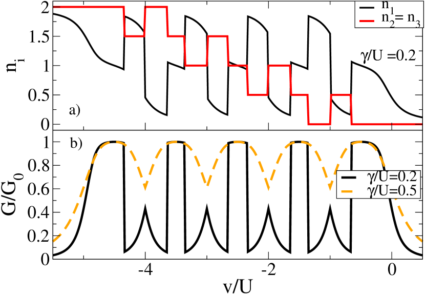
Figure 8: Densities and electrical conductance of the triple quantum dot as function of the gate level for the fully degenerate case and $\gamma/U=0.2$.

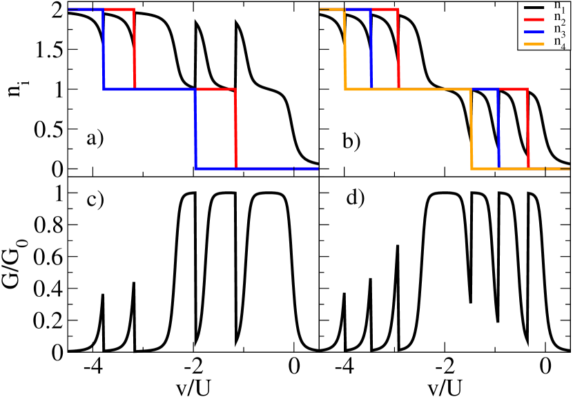
Figure 9: DFT densities and zero-bias conductance as function of the gate level. Panels a) and c): Triple quantum dot with $U=\frac{5}{4}U_{12}=\frac{5}{3}U_{13}=2U_{23}$ and $v=v_{1}=v_{2}-0.1=v_{3}-0.4$. Panels b) and d): Quadruple quantum dot with $U=U_{i}=2U_{ij}$ for all $i\neq j$ and $v=v_{1}=v_{2}-0.02=v_{3}-0.02=v_{4}-0.04$. In both cases we chose $U=10\gamma$.

V Conclusions

In this work we have studied from a DFT perspective the LOS effect which occurs in multi-orbital quantum dots subject to inter and intra Coulomb repulsions when only one of the dots is coupled to leads. The system can be mapped into an effective SIAM problem for the coupled impurity which experiences an effective gate potential due to electrostatic interactions with the other impurities. The density of the system is obtained by choosing the minimum total energy (expressed in terms of DFT quantities) among the available $3^{M-1}$ different configurations of integer occupation of the uncontacted levels. A LOS event occurs at that gate for which the energy minimum passes from one configuration of integer occupations to another one. We have modified an already quite accurate parametrization of the SIAM Hxc functional in order to correctly capture the coupling strength dependence of the LOS events which is quite sensitive to details of the functional. Our new parametrization yields very small energy differences (of the order of $\sim 10^{-3}U$) as compared to the previous one. This produces almost no effect on the selfconsistent densities of SIAM, but is essential to shift the gates at which the LOS events occur to the correct positions. DFT calculations employing the parametrized Hxc functionals for the double quantum dot show excellent agreement with many-body NRG calculations. We have further presented results for the triple and quadruple quantum dot.

VI Acknowledgments

We acknowledge funding through the grant “Grupos Consolidados UPV/EHU del Gobierno Vasco” (IT1453-22). We also acknowledges funding through a grant of the ”Ministerio de Ciencia y Innovación (MCIN)” (Grant No. PID2020-112811GB-I00).

Appendix A Kinetic energy of a non-interacting impurity coupled to two leads

The purpose of this Appendix is to derive the explicit functional of the non-interacting kinetic energy of a non-interacting impurity connected to left (L) and right (R) leads. We start by writing the Hamiltonian of this non-interacting impurity in second quantized form as

$$\hat{H}=v_{s}\hat{d}^{\dagger}\hat{d}+\sum_{\alpha=L,R}\sum_{k\sigma}\epsilon_{\alpha k}\hat{c}^{\dagger}_{\alpha k\sigma}\hat{c}_{\alpha k\sigma}+\hat{H}_{\rm kin}$$ (14)

where

$$\hat{H}_{\rm kin}=\sum_{\alpha=L,R}\sum_{k\sigma}\left(V_{\alpha k,d}\hat{d}^{\dagger}_{\sigma}\hat{c}_{\alpha k\sigma}+{\rm H.c.}\right)\;.$$ (15)

The (non-interacting) kinetic energy is then given as

$$T_{s}=\langle\hat{H}_{\rm kin}\rangle=2\sum_{\alpha k}\left(-iV_{\alpha k,d}G_{\alpha k,d}^{<}(t^{+},t)+{\rm c.c.}\right)$$ (16)

where the prefactor two comes from spin

$$G_{\alpha k,d}^{<}(t,t^{\prime})=i\langle\hat{d}^{\dagger}_{\sigma,H}(t^{\prime})\hat{c}_{\alpha k\sigma,H}(t)\rangle$$ (17)

is the (spin-independent) matrix element of the lesser Green function between single-particle basis states $|\alpha k\sigma\rangle$ and $|d\sigma\rangle$. By standard Green function techniques [55] Eq. 16 can be written as

$$T_{s}=2\sum_{\alpha k}\left(V_{\alpha k,d}\int_{-\varepsilon_{C}}^{0}\frac{{\rm d}\omega}{2\pi}A_{\alpha k,d}(\omega)+{\rm c.c.}\right)$$

$$=2\sum_{\alpha k}\left(V_{\alpha k,d}\int_{-\varepsilon_{C}}^{0}\frac{{\rm d}\omega}{2\pi}i(G_{\alpha k,d}^{R}(\omega)-G_{\alpha k,d}^{A}(\omega))+{\rm c.c.}\right)$$

where $G^{R}$ ($G^{A}$) are the retarded (advanced) Green functions and we introduced an energy cutoff $\varepsilon_{C}$ in order for the integral to converge. The retarded Green function $\hat{G}^{R}(\omega)$ at energy $\omega$ is defined through [55, 44]

$$\left((\omega+i\eta)\hat{\mathbb{I}}-\hat{H}\right)\hat{G}^{R}(\omega)=\hat{\mathbb{I}}.$$ (19)

In the single-particle basis, all Hamiltonian matrix elements directly connecting left and right leads vanish, i.e., $\langle Lk\sigma|\hat{H}|Rk^{\prime}\sigma^{\prime}\rangle=\langle Rk\sigma|\hat{H}|Lk^{\prime}\sigma^{\prime}\rangle=0$. Then, from Eq. 19 one can derive

$$G_{\alpha k,d}^{R}(\omega)=\frac{V_{\alpha k,d}^{*}}{\omega-\epsilon_{k}+i\eta}G_{d}(\omega)$$ (20)

$$G_{d}^{R}(\omega)=\frac{1}{\omega-v_{s}-\Delta^{R}(\omega)}$$ (21)

with $\eta\to 0^{+}$ and $\Delta^{R}(\omega)=\sum_{\alpha}\Delta_{\alpha}^{R}(\omega)$ is the total embedding self energy with

$$\Delta_{\alpha}^{R}(\omega)=\sum_{k}\frac{|V_{\alpha k,d}|^{2}}{\omega-\varepsilon_{\alpha k}+i\eta}$$ (22)

In the wide-band limit we have $\Delta_{\alpha}^{R}(\omega)=-i\frac{\gamma_{\alpha}}{2}$, independent of $\omega$. Inserting Eqs. (20) and (22) into LABEL:Ts_kin2 we arrive at

$$T_{s}=\frac{\gamma}{\pi}\int_{-\varepsilon_{C}}^{0}{\rm d}\omega\;{\rm Re}[G_{d}^{R}(\omega)]=\frac{\gamma}{2\pi}\log\left[\frac{v_{s}^{2}+\frac{\gamma^{2}}{4}}{\varepsilon_{C}^{2}+\frac{\gamma^{2}}{4}}\right]$$ (23)

The non-interacting density-potential relation is

$$n=1-\frac{2}{\pi}\arctan\left(\frac{2v_{s}}{\gamma}\right)$$ (24)

which can easily be inverted to give

$$v_{s}=\frac{\gamma}{2}\tan\left(\frac{\pi}{2}(1-n)\right)\;.$$ (25)

Inserting Eq. 25 into Eq. 23 then gives the final result for the non-interacting kinetic energy functional

$$T_{s}[n]=\frac{\gamma}{2\pi}\log\left[\frac{\frac{\gamma^{2}}{4}\left(\tan{\left(\frac{\pi}{2}(1-n)\right)}^{2}+1\right)}{\varepsilon_{C}^{2}+\frac{\gamma^{2}}{4}}\right].$$ (26)

References

- Petta and Ralph [2001] J. R. Petta and D. C. Ralph, Phys. Rev. Lett. 87, 266801 (2001).
- Hanson et al. [2007] R. Hanson, L. P. Kouwenhoven, J. R. Petta, S. Tarucha, and L. M. K. Vandersypen, Rev. Mod. Phys. 79, 1217 (2007).
- Nygård et al. [2000] J. Nygård, D. H. Cobden, and P. E. Lindelof, Nature 408, 342 (2000).
- Buitelaar et al. [2002] M. R. Buitelaar, A. Bachtold, T. Nussbaumer, M. Iqbal, and C. Schönenberger, Phys. Rev. Lett. 88, 156801 (2002).
- Park et al. [2002] J. Park, A. N. Pasupathy, J. I. Goldsmith, C. Chang, Y. Yaish, J. R. Petta, M. Rinkoski, J. P. Sethna, H. D. Abruña, P. L. McEuen, and D. C. Ralph, Nature 417, 722 (2002).
- Hewson [1997] A. C. Hewson, The Kondo problem to heavy fermions (Cambr. Univ. Press, Cambridge, 1997).
- Averin and Likharev [1986] D. V. Averin and K. K. Likharev, Journal of Low Temperature Physics 62, 345 (1986).
- Shtrikman et al. [1998] H. Shtrikman, D. Mahalu, D. Abusch-Magder, U. Meirav, M. A. Kastner, and D. Goldhaber-Gordon, Nature 391, 156 (1998).
- Goldhaber-Gordon et al. [1998] D. Goldhaber-Gordon, J. Göres, M. A. Kastner, H. Shtrikman, D. Mahalu, and U. Meirav, Phys. Rev. Lett. 81, 5225 (1998).
- Champagne et al. [2005] A. R. Champagne, A. N. Pasupathy, and D. C. Ralph, Nano Lett. 5, 305 (2005).
- Parks et al. [2007] J. J. Parks, A. R. Champagne, G. R. Hutchison, S. Flores-Torres, H. D. Abruña, and D. C. Ralph, Phys. Rev. Lett. 99, 026601 (2007).
- Jarillo-Herrero et al. [2005] P. Jarillo-Herrero, J. Kong, H. S. J. van der Zant, C. Dekker, L. P. Kouwenhoven, and S. DeFranceschi, Nature 434, 484 (2005).
- Roch et al. [2009] N. Roch, S. Florens, T. A. Costi, W. Wernsdorfer, and F. Balestro, Phys. Rev. Lett. 103, 197202 (2009).
- Parks et al. [2010] J. J. Parks, A. R. Champagne, T. A. Costi, W. W. Shum, A. N. Pasupathy, E. Neuscamman, S. Flores-Torres, P. S. Cornaglia, A. A. Aligia, C. A. Balseiro, G. K.-L. Chan, H. D. Abruña, and D. C. Ralph, Science 328, 1370 (2010).
- Avinun-Kalish et al. [2005] M. Avinun-Kalish, M. Heiblum, O. Zarchin, D. Mahalu, and V. Umansky, Nature 436, 529 (2005).
- Yacoby et al. [1995] A. Yacoby, M. Heiblum, D. Mahalu, and H. Shtrikman, Phys. Rev. Lett. 74, 4047 (1995).
- Schuster et al. [1997] R. Schuster, E. Buks, M. Heiblum, D. Mahalu, V. Umansky, and H. Shtrikman, Nature 385, 417 (1997).
- Aikawa et al. [2004] H. Aikawa, K. Kobayashi, A. Sano, S. Katsumoto, and Y. Iye, J. Phys. Soc. Jpn. 73, 3235 (2004).
- Ji et al. [2002] Y. Ji, M. Heiblum, and H. Shtrikman, Phys. Rev. Lett. 88, 076601 (2002).
- Zaffalon et al. [2008] M. Zaffalon, A. Bid, M. Heiblum, D. Mahalu, and V. Umansky, Phys. Rev. Lett. 100, 226601 (2008).
- Lim et al. [2006] J. S. Lim, M.-S. Choi, M. Choi, R. López, and R. Aguado, Phys. Rev. B 74, 205119 (2006).
- Kleeorin and Meir [2017a] Y. Kleeorin and Y. Meir, Phys. Rev. B 96, 045118 (2017a).
- Büsser et al. [2011] C. Büsser, E. Vernek, P. Orellana, G. Lara, E. Kim, A. Feiguin, E. Anda, and G. Martins, Phys. Rev. B 83, 125404 (2011).
- Roura-Bas et al. [2011] P. Roura-Bas, L. Tosi, A. Aligia, and K. Hallberg, Phys. Rev. B 84, 073406 (2011).
- Weymann et al. [2018] I. Weymann, R. Chirla, P. Trocha, and C. P. Moca, Phys. Rev. B 97, 085404 (2018).
- Silvestrov and Imry [2007] P. Silvestrov and Y. Imry, New J. Phys. 9, 125 (2007).
- Hohenberg and Kohn [1964] P. Hohenberg and W. Kohn, Phys. Rev 136, B864 (1964).
- Kohn and Sham [1965] W. Kohn and L. J. Sham, Phys. Rev. 140, A1133 (1965).
- Dreizler and Gross [1990] R. M. Dreizler and E. K. U. Gross, Density Functional Theory (Springer, Berlin, 1990).
- J.P. Perdew [1985] J.P. Perdew, Phys. Rev. Lett. 55, 1665 (1985).
- Becke [1988] A. D. Becke, Phys. Rev. A 38, 3098 (1988).
- Perdew et al. [1996] J. P. Perdew, K. Burke, and M. Ernzerhof, Phys. Rev. Lett. 77, 3865 (1996).
- A.D. Becke [1993] A.D. Becke, J. Chem. Phys. 98, 5648 (1993).
- Stefanucci and Kurth [2011] G. Stefanucci and S. Kurth, Phys. Rev. Lett. 107, 216401 (2011).
- Bergfield et al. [2012] J. P. Bergfield, Z.-F. Liu, K. Burke, and C. A. Stafford, Phys. Rev. Lett. 108, 066801 (2012).
- Tröster et al. [2012] P. Tröster, P. Schmitteckert, and F. Evers, Phys. Rev. B 85, 115409 (2012).
- Lima et al. [2002] N. A. Lima, L. N. Oliveira, and K. Capelle, Europhys. Lett. 60, 601 (2002).
- Jacob and Kurth [2018] D. Jacob and S. Kurth, Nano Lett. 18, 2086 (2018).
- Kurth et al. [2019] S. Kurth, D. Jacob, N. Sobrino, and G. Stefanucci, Phys. Rev. B 100, 085114 (2019).
- Jacob et al. [2020] D. Jacob, G. Stefanucci, and S. Kurth, Phys. Rev. Lett. 125, 216401 (2020).
- Sobrino et al. [2020] N. Sobrino, S. Kurth, and D. Jacob, Phys. Rev. B 102, 035159 (2020).
- Perdew et al. [1982] J. P. Perdew, R. Parr, M. Levy, and J. L. Balduz, Phys. Rev. Lett. 49, 1691 (1982).
- Kurth and Stefanucci [2016a] S. Kurth and G. Stefanucci, Phys. Rev. B 94, 241103(R) (2016a).
- Kurth and Stefanucci [2017] S. Kurth and G. Stefanucci, J. Phys.: Condens. Matter 29, 413002 (2017).
- Note [1] See, e.g., Ch. 5.2 in the book by Hewson[6].
- Mera et al. [2010] H. Mera, K. Kaasbjerg, Y. Niquet, and G. Stefanucci, Phys. Rev. B 81, 035110 (2010).
- Langreth [1966] D. C. Langreth, Phys. Rev. 150, 516 (1966).
- Mera and Niquet [2010] H. Mera and Y. Niquet, Phys. Rev. Lett. 105, 216408 (2010).
- Stefanucci and Kurth [2015] G. Stefanucci and S. Kurth, Nano Lett. 15, 8020 (2015).
- Sobrino et al. [2021] N. Sobrino, F. Eich, G. Stefanucci, R. D’Agosta, and S. Kurth, Phys. Rev. B 104, 125115 (2021).
- Sobrino et al. [2019] N. Sobrino, R. D’Agosta, and S. Kurth, Phys. Rev. B 100, 195142 (2019).
- Kurth and Stefanucci [2016b] S. Kurth and G. Stefanucci, Phys. Rev. B 94, 241103(R) (2016b).
- Stefanucci and Kurth [2013] G. Stefanucci and S. Kurth, phys. stat. sol. (b) 250, 2378 (2013).
- Kleeorin and Meir [2017b] Y. Kleeorin and Y. Meir, Phys. Rev. B 96, 045118 (2017b).
- Stefanucci and van Leeuwen [2013] G. Stefanucci and R. van Leeuwen, Nonequilibrium Many-Body Theory of Quantum Systems: A Modern Introduction (Cambridge University Press, 2013).