FreeGaze: Resource-efficient Gaze Estimation via Frequency Domain Contrastive Learning

Abstract.

Gaze estimation is of great importance to many scientific fields and daily applications, ranging from fundamental research in cognitive psychology to attention-aware mobile systems. While recent advancements in deep learning have yielded remarkable successes in building highly accurate gaze estimation systems, the associated high computational cost and the reliance on large-scale labeled gaze data for supervised learning place challenges on the practical use of existing solutions. To move beyond these limitations, we present FreeGaze, a resource-efficient framework for unsupervised gaze representation learning. FreeGaze incorporates the frequency domain gaze estimation and the contrastive gaze representation learning in its design. The former significantly alleviates the computational burden in both system calibration and gaze estimation, and dramatically reduces the system latency; while the latter overcomes the data labeling hurdle of existing supervised learning-based counterparts, and ensures efficient gaze representation learning in the absence of gaze label. Our evaluation on two gaze estimation datasets shows that FreeGaze can achieve comparable gaze estimation accuracy with existing supervised learning-based approach, while enabling up to 6.81 and 1.67 times speedup in system calibration and gaze estimation, respectively.

1. Introduction

Human gaze indicates where the subject is looking at, and is widely considered as an important non-verbal communication cue that expresses the subject’s desires, needs, cognitive stages, and interpersonal relations (hansen2009eye, ). The estimation of human gaze, thus, is of great importance to a wide range of scientific fields (eckstein2017beyond, ). For instance, in cognitive psychology, human gaze provides unique insights into the understanding of mental disorders (shishido2019application, ; duan2019dataset, ), personality traits (berkovsky2019detecting, ), cognitive workload (kosch2018your, ; fridman2018cognitive, ), and visual perception (de2019individual, ; najemnik2005optimal, ).

Beyond the benefits to fundamental science, there is also an unprecedented demand for eye tracking in mobile systems. In the context of virtual and augmented reality (AR/VR), accurate and fast gaze estimation is crucial for ensuring immersive user experiences. Examples such as eye tracking-based dynamic scene adaptation (marwecki2019mise, ) and foveated rendering (patney2016towards, ; kim2019foveated, ). Outside the field of AR/VR, general-purpose RGB cameras, such as those embedded in smartphones (valliappan2020accelerating, ), tablets (wood2014eyetab, ), and webcams (sugano2016aggregaze, ), can also be used to capture facial images of the user and enable appearance-based gaze estimation systems (cheng2021appearance, ). In fact, gaze has been used to improve user perceived quality in webpage loading (kelton2017improving, ), to recognize daily human activity (lan2020gazegraph, ; srivastava2018combining, ), and to ensure friendly human-robot interaction (gillet2021robot, ; weldon2021exploring, ). Despite the numerous benefits, there are two practical challenges that hinder the wide adoption of existing gaze estimation solutions.

Challenges in collecting large-scale labeled gaze data. Similar to the other computer vision tasks, the advancements in convolutional neural networks (CNN) have contributed significantly to the success in gaze estimation (kassner2014pupil, ; cheng2021appearance, ; zhang2020eth, ; krafka2016eye, ; zhang2018training, ; zhang2017mpiigaze, ; huynh2021imon, ). However, like many CNN-based systems, existing gaze estimation solutions rely on supervised learning, and thus, their performance is largely depending on the availability of a large-scale, well-labeled training dataset. Unfortunately, collecting gaze data with accurately annotated labels is a labor-intensive and impractical process that requires controlled and highly sophisticated setups and subject recruitment (kellnhofer2019gaze360, ; zhang2017mpiigaze, ; zhang2020eth, ; newman2020turkeyes, ). For instance, existing gaze datasets are collected using expensive, high-resolution cameras (kellnhofer2019gaze360, ; zhang2017mpiigaze, ; zhang2020eth, ), or relying on dedicated crowdsourcing platforms (krafka2016eye, ; newman2020turkeyes, ). What makes the gaze data collection more challenging is that the accuracy of gaze annotation is highly influenced by the user’s fixation ability and cooperation during the collection process (openeds, ). For example, due to the subconscious eye movements, the participant may not gaze at the “ground-truth” point that she supposed to fixed on, and thus, leads to incorrect gaze labels and dirty data. Therefore, while complex CNN models are worthwhile for ensuring high gaze estimation accuracy, we need an efficient and inexpensive solution to train the system, in the absence of gaze label.

Challenges in system latency. The adoption of complex neural networks also introduces high system latency in both calibration and gaze estimation stages, which places limitations on the practical use of existing solutions.

First, to eliminate the impact of subject diversity on the gaze estimation accuracy, all existing solutions need to perform the subject-specific calibration before the system’s first use (hansen2009eye, ; cheng2021appearance, ; sugano2015self, ; lanata2015robust, ; linden2019learning, ). The calibration fine-tunes the pre-trained gaze estimation model by a small set of labeled gaze data collected from the targeted subject on the fly. Thus, when complex neural networks are employed (cheng2021appearance, ), the online calibration becomes a time-consuming process and affects the user’s experience. Indeed, our measurement study (Section 5.4) indicates that a ResNet-18 based solution (which is 32-layers shallower than the ResNet-50 based design that is widely adopted by existing solutions (zhang2020eth, )) takes 10.2 minutes for calibration, despite a high-end GeForce RTX 3080Ti GPU is used. Note that, calibration is also inevitable for high-end model-based eye tracking systems, e.g., Tobii Pro (tobiiCalibration, ), Pupil Lab (pupilLabCalibration, ), and VIVE Pro Eye VR headset (vevoCalibration, ), though their calibration is performed in a slightly different way.

Second, mobile systems usually have a constrained time budget for run-time gaze estimation. For instance, foveated rendering (patney2016towards, ; kim2019foveated, ) requires a low gaze estimation latency to render a high-quality image precisely in the user’s foveal vision on time, even when the user is making fast eye movements such as saccades (albert2017latency, ). Similarly, eye tracking-based psychological applications (mele2012gaze, ) require a high tracking rate to capture fine-grained cognitive contexts. Thus, in practical application scenario, gaze estimation systems often face the requirements of low inference latency.

To address these challenges, we present FreeGaze, a resource-efficient framework for unsupervised gaze representation learning. At the core of FreeGaze are the frequency domain gaze estimation and the contrastive gaze representation learning. The former significantly alleviates the computational burden in both calibration and estimation, and dramatically reduces the system latency; while the latter overcomes the data labeling hurdle of existing supervised learning-based counterparts, and ensures efficient gaze representation learning without gaze label. These capabilities are made possible by a suite of novel techniques devised in this work.

First, existing gaze estimation systems take RGB images as inputs. To reduce the system latency, a straightforward way is to aggressively reduce the input size of the neural networks. However, simply compressing or downsampling the RGB image will destroy the perceptual information it contains and leads to poor estimation performance. To resolve this challenge, we introduce the frequency domain gaze estimation (Section 4.5), which employs the discrete cosine transform (DCT) to convert the original RGB images to the frequency domain, and takes the DCT coefficients as inputs for gaze estimation. Moreover, we exploit the spectral compaction property (rao2014discrete, ) of the DCT, which concentrates the critical content-defining information of the image in the low-end of the frequency spectrum, while putting the trivial and noise signals in the high-frequency end (wallace1991jpeg, ). This motivates us to aggressively compact the essential perceptual information in the RGB image into a few DCT coefficients in the low-frequency domain. In fact, as demonstrated in Section 5, when comparing with conventional RGB-based solutions, the proposed frequency domain gaze estimation achieves up to 6.81 and 1.67 times speedup in calibration and gaze estimation, respectively.

Second, to overcome the data labeling hurdle of existing supervised gaze estimation systems (kassner2014pupil, ; zhang2020eth, ; krafka2016eye, ; zhang2018training, ; zhang2017mpiigaze, ; huynh2021imon, ), we propose a contrastive learning (CL)-based framework (Section 4.2) that leverages unlabeled facial images for gaze representation learning. Although various CL-based unsupervised learning methods have been proposed for general purpose visual tasks, such as image classification (chen2020simple, ; dosovitskiy2014discriminative, ) and object detection (xie2021detco, ), they are ill-suited for gaze estimation, as they focus on learning general representations that are more related to the appearance and the identity of the subjects. In fact, as demonstrated in Sections 3 and 5, conventional CL approach, i.e., SimCLR (chen2020simple, ), can lead to poor performance in gaze representation learning and high gaze estimation error. To resolve this challenge, we devise a set of techniques for contrastive gaze representation learning. Specifically, we introduce the subject-specific negative pair sampling strategy (Section 4.3) to encourage the learning of gaze-related features, and design the gaze-specific data augmentation (Section 4.4) to ensure the gaze consistence during the contrastive learning. As demonstrated (Section 5.3), the two techniques lead to significant improvements in gaze estimation when comparing with the conventional unsupervised method (chen2020simple, ).

Our major contributions are summarized as follows:

• We introduce the frequency domain gaze estimation that exploits the spectral compaction property of the discrete cosine transform to aggressively compress the inputs of gaze estimation systems and achieves significant speedup in both calibration and gaze estimation stages. To our best knowledge, this is the first work that leverages the DCT coefficients for gaze estimation.

• We propose the frequency domain contrastive gaze representation learning framework that overcomes the data labeling hurdle of existing supervised learning-based counterparts. We devise the subject-specific negative pair sampling strategy and the gaze-specific data augmentation to ensure efficient self-supervised gaze representation learning.

• We conduct a comprehensive evaluation of FreeGaze on two state-of-the-art gaze estimation datasets. The results demonstrate the effectiveness of FreeGaze in learning gaze representations in the compressed frequency domain. Specifically, FreeGaze reduces the angular error of the conventional CL-based method by 5.4^∘ and 4.6^∘ on average over the two datasets, respectively. When comparing with the RGB supervised learning-based method, which takes 37K and 30K labeled images for training, FreeGaze achieves comparable results, i.e., the performance gap is only 1.1^∘ and 1.6^∘ on average over the two datasets, while enabling up to 6.81 and 1.67 times speedup in calibration and gaze estimation, respectively.

The rest of the paper is organized as follows. We review related work in Section 2. We introduce the motivation and challenges in Section 3. The design details of FreeGaze are given in Section 4. We evaluate our work in Section 5 followed by the conclusion in Section 6.

2. Related Work

2.1. Gaze Estimation

Existing gaze estimation systems can be classified into model-based and appearance-based methods. Model-based estimation systems extract features from eye images to fit a geometric model that predicts gaze direction (hansen2009eye, ). However, they require dedicated eye tracking camera (kassner2014pupil, ; nakazawa2012point, ; guestrin2006general, ) to capture near-eye images for the estimation, which hinders their pervasive adoption. By contrast, appearance-based solutions rely on ordinary facial or eye images captured by general-purpose RGB cameras, such as those embedded in smartphones (valliappan2020accelerating, ; krafka2016eye, ), tablets (wood2014eyetab, ; zhang2018training, ), and public displays (sugano2016aggregaze, ; zhang2015appearance, ), which makes them promising for a wide range of everyday settings. The latest appearance-based gaze estimation systems benefit from the representation learning capability of deep neural networks, and have shown promising performance that significantly surpassed their model-based counterparts (cheng2021appearance, ). Indeed, over the last couple of years, a plethora of deep learning-based gaze estimation solutions have been proposed (valliappan2020accelerating, ; krafka2016eye, ; zhang2018training, ; zhang2017mpiigaze, ; zhang2020eth, ; huynh2021imon, ). For instance, Zhang et al. (zhang2015appearance, ) took eye images and head pose information estimated from facial images as inputs to train a multi-modal CNN for gaze estimation. They also showed that adopting a deeper neural networks, i.e., the ResNet-50, can further improve the estimation accuracy (zhang2017mpiigaze, ; zhang2020eth, ).

Despite the promise of recent deep learning-based solutions, they rely on supervised learning and require a large labeled gaze dataset for training, e.g., 210K images for the MPIIGaze (zhang2017mpiigaze, ) and 750K images for the ETH-XGaze (zhang2020eth, ), which is complex and expensive to be collected and annotated. By contrast, FreeGaze achieves gaze estimation in an unsupervised manner. Moreover, by taking frequency domain representations as inputs, FreeGaze achieves up to 6.81 and 1.67 times speedup in system calibration and inference, respectively, when comparing with the conventional RGB-based gaze estimation solution.

2.2. Unsupervised Representation Learning

Our work is also related to existing efforts in unsupervised representation learning, which can be roughly categorized into generative and discriminative methods. Generative methods usually take the form of auto-encoder (le2013building, ; kingma2013auto, ) or generative adversarial network (radford2015unsupervised, ), and learn the feature embedding network by reconstructing the original high-dimensional inputs from the low-dimensional latent representations. However, generative methods perform pixel-level image reconstruction that is computationally expensive (grill2020bootstrap, ). By contrast, discriminative methods learn representations by solving different pretext tasks, such as recognizing the rotation of the image  (gidaris2018unsupervised, ), solving jigsaw puzzles (noroozi2016unsupervised, ), and contrastive prediction task (ye2019unsupervised, ). Among them, contrastive prediction task-based solutions currently achieve state-of-the-art performance in unsupervised representation learning for a wide range of tasks, such as image classification (chen2020simple, ; dosovitskiy2014discriminative, ) and object detection (xie2021detco, ). However, as discussed in Sections 3 and 5, conventional contrastive learning approaches focus on learning general representations that are more related to the appearance and the identity of the subjects, which leads to poor performance on gaze estimation. By contrast, FreeGaze incorporates a set of techniques that encourage the learning of gaze-related features to improve gaze estimation performance.

There are also works on unsupervised gaze representation learning. Yu et al. (yu2020unsupervised, ) proposed a method to learn low dimensional gaze representations by jointly training a gaze redirection network (yu2019improving, ) and a gaze representation network. However, the training of the gaze redirection network requires well aligned eye images, setting constraints on their approach. More recently, by constructing eye-consistent and gaze-similar image pairs, Sun et al. (sun2021cross, ) proposed the cross-encoder to learn gaze representations from unlabeled eye images. These two solutions rely on generative models for representation learning, which requires the computationally expensive pixel-level image reconstruction. By contrast, FreeGaze builds upon contrastive learning to avoid the reconstruction process.

2.3. Learning in the Frequency Domain

FreeGaze is also related to existing efforts in using compressed frequency domain representations for image-based learning tasks (delac2009face, ; hafed2001face, ; ghosh2016deep, ; ehrlich2019deep, ; chamain2020improving, ; xu2020learning, ). Delac et al. (delac2009face, ) investigated the feasibility of using the DCT and the discrete wavelet transform (DWT) coefficients in the JEPG and JEPG2000 compressed domain for face recognition. In the deep learning regime, Ghosh and Chellappa (ghosh2016deep, ) demonstrated that by leveraging the feature extraction capability of DCT and incorporating DCT operation on the feature maps generated by the convolutional layers, one can speed up the network convergence during training. Gueguen et al. (gueguen2018faster, ) suggested that when using the DCT coefficients as the inputs, the first fewer layers of CNN can be pruned to improve computational efficiency. Distinct from existing works, we exploit the spectral compaction property of DCT for aggressive input compression, and are the first to investigate unsupervised learning in the frequency domain for gaze estimation.

3. Challenges

3.1. Challenges in Unsupervised Gaze Representation Learning

Motivated by recent advances in contrastive visual representation learning (chen2020simple, ; dosovitskiy2014discriminative, ; henaff2020data, ; he2020momentum, ), we propose a contrastive learning (CL)-based framework for gaze representation learning. However, existing CL methods are designed for general purpose visual tasks, such as image classification (chen2020simple, ; dosovitskiy2014discriminative, ) and object detection (xie2021detco, ), which cannot be used directly for gaze estimation. This is because, for general purpose tasks, existing solutions aim to identify a feature embedding network that ensures the feature representations of visually similar images, i.e., images contain the same object instance or objects of the same category (wang2016contextual, ), are close to each other in the low-dimensional embedding space (hadsell2006dimensionality, ), while the feature representations of visually distinct images are as separated as possible (ye2019unsupervised, ). Unfortunately, for gaze estimation, facial images with the same gaze label can be visually distinct, which makes the conventional contrastive learning methods ill-suited for gaze estimation.

As an example, Figure 1 shows three facial images labeled with the corresponding gaze direction. Figures 1(a) and (b) belong to the same subject, but have different gaze directions. In comparison, Figures 1(b) and (c) belong to different subjects, but have the same gaze direction. Conventional CL methods will treat the first two images as a visually similar pair, as they contain the same subject with highly similar appearance, while consider the latter two as a visually distinct pair, as they contain different subjects. As a result, the embedding network will learn representations that are related to subject identity, which are ill-suited for gaze estimation.

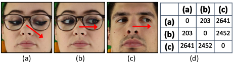
Figure 1. Examples of facial image labeled with gaze direction (red arrow): (a) and (b) are facial images of the same subject but have different gaze directions; in comparison, (b) and (c) are facial images of different subjects but have the same gaze direction; (d) shows the Euclidean distance between the learned representations of the three facial image pairs.

To demonstrate, we adopt the widely used contrastive learning framework SimCLR (chen2020simple, ) to train a ResNet-18 based (he2016deep, ) embedding network for unsupervised representation learning. We use the ETH-XGaze (zhang2020eth, ) as the training dataset. After training, we take the three facial images shown in Figures 1(a)-(c) as the inputs of the embedding network to obtain the corresponding representations. Finally, we measure the Euclidean distance between the representations of the three images. The results are shown in Figure 1(d). The distance between image pair $(b,c)$ is 12 times larger than that of image pair $(a,b)$, even though $(b,c)$ have the same gaze direction. This indicates that the embedding network trained by SimCLR tends to push the representations of the visually similar image pair $(a,b)$ close to each other in the embedding space, while separate the representations of the visually distinct image pair $(b,c)$ apart. As shown in Section 5.3, conventional contrastive learning will lead to high error in gaze estimation.

3.2. Challenges in System Latency

In addition to the data challenge, the associated high system latency also hinders the pervasive adoption of existing solutions.

Calibration latency. The first type of latency is introduced by the calibration process of gaze estimation system. Subjects have large diversity in their eye shapes and inner eye structures (levin2011adler, ), which introduces a non-negligible impact on the appearance of eyes and makes it difficult to build a “one size fits all” gaze estimation model. A widely adopted remedy for this problem is to perform subject-specific calibration before the system’s first use (hansen2009eye, ; sugano2015self, ; lanata2015robust, ; linden2019learning, ). Note that, even for the commercial high-end eye tracking systems, e.g., Tobii Pro (tobiiCalibration, ), Pupil Lab (pupilLabCalibration, ), and VIVE Pro Eye VR headset (vevoCalibration, ), subject-specific calibration is also inevitable to ensure good gaze estimation accuracy. For deep learning-based systems, the calibration requires fine-tuning the pre-trained gaze estimation model by a small set of labeled gaze data collected from the targeted subject on the fly. Moreover, given the fact that state-of-the-art gaze estimation systems adopt complex neural networks (cheng2021appearance, ), e.g., ResNet-50 (zhang2020eth, ) and VGG-16 (zhang2017mpiigaze, ), as the backbone network, the online calibration becomes a time-consuming process and affects the user’s experience and acceptance of the system, especially when limited computational resource is available.

Inference latency. Similar to the time demand in calibration, gaze estimation systems also have a constrained time budget for inference. Low inference latency is desirable for a wide range of applications, e.g., foveated rendering in virtual reality (konrad2020gaze, ; albert2017latency, ), and eye tracking-based psychological research (mele2012gaze, ).

In Section 5.4, our latency evaluation shows that a ResNet-18 based solution (which is 32-layers shallower than the ResNet-50 based design that is widely adopted by existing solutions (zhang2020eth, )) takes 10.2 minutes for calibration, despite a high-end GeForce RTX 3080Ti GPU is used. By contrast, our proposed FreeGaze can bring the latency down to 1.8 minutes, which is a 5.67 times speedup. Similarly, for inference, FreeGaze achieves at least 1.59 times speedup when comparing with the conventional method.

4. System Design

4.1. Overview

In this work, we present FreeGaze, a resource-efficient unsupervised learning framework for gaze estimation. At the core of FreeGaze are the frequency domain gaze estimation and the contrastive gaze representation learning: the former dramatically reduces the latency in both system calibration and gaze estimation to ensure high time efficiency; while the latter overcomes the data labeling hurdle of existing supervised learning-based counterparts to ensure gaze representation learning without gaze label. The overview design of FreeGaze is shown in Figure 2, which includes three stages: the self-supervised pre-training stage, the supervised calibration stage, and the deployment stage.

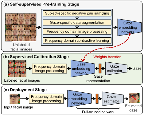
Figure 2. Overview of FreeGaze which incorporates: (a) the self-supervised pre-training stage; (b) supervised calibration stage; and (c) deployment stage.

In the self-supervised pre-training stage, FreeGaze takes unlabeled facial images as inputs to pre-train a gaze embedding network (Section 4.6) for unsupervised gaze representation learning. Specifically, we achieve this by a comprehensive set of techniques devised in this work, including: (1) the subject-specific negative pair sampling strategy (Section 4.3) that encourages the gaze embedding network to learn gaze-related features and abandon identity or appearance-related features; (2) the gaze-specific data augmentation (Section 4.4) that maintains the gaze-related semantic features in the augmented positive image pairs; (3) the frequency domain image processing module (Section 4.5) that selects the essential DCT coefficients of the original RGB facial images to reduce the computation latency in both calibration and deployment stages; and (4) the frequency domain contrastive learning module that leverages the DCT coefficients as the inputs to train the gaze embedding network.

After the contrastive learning, the pre-trained gaze embedding network is transferred to the supervised calibration stage, and serves as a feature extractor for the downstream gaze estimation task. Specifically, taking a small amount of labeled facial images from the targeted subject as inputs, we first leverage the frequency domain image processing module to obtain the DCT coefficients of the original RGB images. Then, we fine-tune the pre-trained gaze embedding network and the gaze estimator for subject-specific gaze estimation. Note that, as mentioned in Section 3.2, the subject-specific calibration is essential to ensure good gaze estimation accuracy, even for high-end eye tracking systems. Finally, in the deployment stage, the fine-tuned gaze embedding network and the gaze estimator are used for run-time gaze estimation.

Below, we present the detailed design of FreeGaze. We first introduce the pipeline of the frequency domain contrastive learning framework, followed by the designs of each individual components.

4.2. Frequency Domain Contrastive Gaze Representation Learning

Inspired by recent advances in contrastive visual representation learning (chen2020simple, ; dosovitskiy2014discriminative, ; henaff2020data, ; he2020momentum, ), we propose the frequency domain contrastive learning to train the gaze embedding network. The training is conducted by solving a set of contrastive prediction tasks. More specifically, the gaze embedding network learns the good representations for gaze estimation by maximizing the representation similarity between positive image pairs that have the same gaze direction, while minimizing the representation similarity between negative image pairs that have low gaze similarity. The pipeline of the proposed learning framework is shown in Figure 3, which consists of the following six major components:

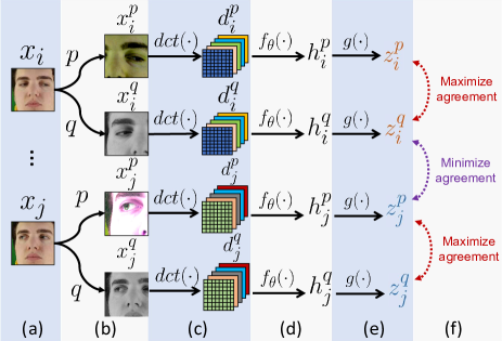
Figure 3. The pipeline of the proposed frequency domain contrastive gaze representation learning framework, which consists of: (a) subject-specific negative pair sampling; (b) stochastic gaze-specific data augmentation; (c) frequency domain image processing; (d) gaze embedding network; (e) projection head; and (f) contrastive prediction task.

(a) Subject-specific negative pair sampling: we first sample a minibatch of $N$ samples, $\{x_{\_}i\}_{\_}{i=1}^{N}$, from the unlabelled facial image set for contrastive learning. Instead of performing random image sampling, we introduce the subject-specific negative pair sampling strategy (in Section 4.3) that encourages the gaze embedding network to focus on gaze-related semantic features for better representation learning. As demonstrated in Section 5.3.3, the proposed sampling strategy improves the gaze estimation accuracy by a large margin when comparing with the conventional method.

(b) Stochastic gaze-specific data augmentation: we then apply the stochastic gaze-specific data augmentation to each image $x_{\_}i$ in the minibatch for two times. Specifically, we transform each $x_{\_}i\in\{x_{\_}i\}_{\_}{i=1}^{N}$ into two correlated views, denoted as $x_{\_}i^{p}$ and $x_{\_}i^{q}$, respectively. As shown in Figure 3, we consider images $x_{\_}i^{p}$ and $x_{\_}i^{q}$, which are augmented from the same facial image $x_{\_}i$, as a positive image pair. By contrast, $x_{\_}i^{q}$ and $x_{\_}j^{p}$, which are augmented from different image samples, are considered as a negative image pair. We introduce a novel gaze-specific data augmentation operator, i.e., gaze-cropping and resizing (in Section 4.4), to maintain the gaze-related semantic features for the augmented images. As demonstrated in Section 5.3, our proposed method leads to better performance in gaze representation learning, and reduces the gaze estimation error by a large margin of 7^∘ in angular error, when comparing with the conventional data augmentation operators (chen2020simple, ).

(c) Frequency domain image processing: to reduce the computation latency in both calibration and gaze inference, we propose to use the DCT coefficients of the original RGB images as the inputs for representation learning. Specifically, we introduce the frequency domain image processing, $dct(\cdot)$, to transform the augmented image, $x_{\_}i^{t}$, from the RGB color space to the DCT frequency domain. The final output $d_{\_}i^{t}$ is the selected DCT coefficients matrix. The detail of the frequency domain image processing is introduced in Section 4.5. As shown in the latency evaluation in Section 5.4, leveraging the DCT coefficients as inputs for representation learning can achieve up to 6.81 and 1.67 times speedup in system calibration and gaze inference, respectively.

(d) Gaze embedding network: then we train a gaze embedding network, $f_{\_}{\theta}(\cdot)$, to map the processed DCT coefficients matrix $d_{\_}i^{t}$ to the gaze representations in the latent space:

(1) $$h_{\_}i^{t}=f_{\_}{\theta}(d_{\_}i^{t})\in\mathbb{R}^{D},\;t\in\{p,q\}\;\textrm{and}\;i\in\{1,..,N\},$$

where $D$ is the dimension of the gaze representations. In Section 4.6, we introduce the design of the gaze embedding network in detail.

(e) Projection head: we then use a nonlinear projection head, $g(\cdot)$, to further transform the gaze representations, $h_{\_}i^{t}$, to a lower dimensional latent space. The projection head is a multi-layer perceptron (MLP) with one hidden layer. The representations, $z_{\_}i^{t}$, after the nonlinear projection can be obtained by:

(2) $$z_{\_}i^{t}=g(h_{\_}i^{t}),\;t\in\{p,q\}\;\textrm{and}\;i\in\{1,..,N\}.$$

The nonlinear projection head can encourage the embedding network $f_{\_}{\theta}(\cdot)$ to form and maintain features that are beneficial for the downstream task (chen2020simple, ; chen2020big, ), which can further improve the quality of the learned representations $h_{\_}i^{t}$.

(f) Contrastive prediction task: the gaze embedding network $f_{\_}{\theta}(\cdot)$ learns the good representations for gaze estimation by maximizing the representation similarity between positive image pairs that have the same gaze direction, while minimizing the representation similarity between negative image pairs that have different gaze directions. In another words, we aim to jointly train $f_{\_}{\theta}(\cdot)$ and $g(\cdot)$ to pull the projected representations of the positive pairs, e.g., $z_{\_}i^{p}$ and $z_{\_}i^{q}$, closer together on the latent space; while pushes the representations of the negative pairs farther apart. This learning objective is achieved by solving the contrastive prediction task on the sampled minibatch $\{x_{\_}i\}_{\_}{i=1}^{N}$. Formally, for two augmented sets $\{x_{\_}i^{p}\}_{\_}{i=1}^{N}$ and $\{x_{\_}i^{q}\}_{\_}{i=1}^{N}$ generated from $\{x_{\_}i\}_{\_}{i=1}^{N}$, the contrastive prediction loss function for a positive pair $(x_{\_}i^{p},x_{\_}i^{q})$ is defined as (wu2018unsupervised, ; chen2020simple, ):

(3) $$\mathcal{L}_{\_}{i,p,q}=-\log{\frac{\exp\Big{(}\text{sim}(z_{\_}i^{p},z_{\_}i^{q})/\tau\Big{)}}{\sum_{\_}{k=1}^{N}{\exp\Big{(}\text{sim}(z_{\_}i^{p},z_{\_}k^{q})/\tau\Big{)}}}},\;i\in\{1,..,N\},$$

where $\text{sim}(u,v)=u^{\top}v/\|u\|\|v\|$ is the cosine similarity of two feature vectors $u$ and $v$, and $\tau$ is a temperature parameter.

The total loss is computed across all positive pairs in $\{x_{\_}i^{p}\}_{\_}{i=1}^{N}$ and $\{x_{\_}i^{q}\}_{\_}{i=1}^{N}$for both $(x_{\_}i^{p},x_{\_}i^{q})$ and $(x_{\_}i^{q},x_{\_}i^{p})$, and can be obtained by:

(4) $$\mathcal{L}=\frac{1}{2N}\sum_{\_}{i=1}^{N}{\Big{(}\mathcal{L}_{\_}{i,p,q}+\mathcal{L}_{\_}{i,q,p}\Big{)}}.$$

Finally, $f_{\_}{\theta}(\cdot)$ and $g(\cdot)$ are jointly trained by minimizing $\mathcal{L}$. When the training is complete, the projection head will be discarded in the supervised calibration stage, and we use the gaze representations, $h_{\_}i^{t}$, as the input for the gaze estimator, which is simply a MLP with one hidden layer.

Below, we introduce the proposed subject-specific negative pair sampling strategy (Section 4.3), stochastic gaze-specific data augmentation (Section 4.4), frequency domain image processing (Section 4.5), and the gaze embedding network (Section 4.6) in detail.

4.3. Subject-specific Negative Pair Sampling

4.3.1. Rationale

Recall our discussion in Section 3.1 that facial images with the same gaze direction can be visually distinct, while visually similar images can have completely different gaze directions (in Figure 1). Thus, to ensure good representation learning for gaze estimation, the gaze embedding network $f_{\_}{\theta}(\cdot)$ should learn representations that are related to the gaze, instead of capturing features that are related to the identity or the appearance of the subjects. As discussed in Section 4.2, $f_{\_}{\theta}(\cdot)$ learns the good representations by minimizing the contrastive loss defined in Equation (3), which can be further extended as:

(5) $$\mathcal{L}_{\_}{i,p,q}=-\log{\frac{\exp\Big{(}\text{sim}(z_{\_}i^{p},z_{\_}i^{q})/\tau\Big{)}}{\exp\Big{(}\text{sim}(z_{\_}i^{p},z_{\_}i^{q})/\tau\Big{)}+\sum_{\_}{k\neq i}^{N}{\exp\Big{(}\text{sim}(z_{\_}i^{p},z_{\_}k^{q})/\tau\Big{)}}}}.$$

Clearly, minimizing $\mathcal{L}_{\_}{i,p,q}$ requires maximizing $\exp(\text{sim}(z_{\_}i^{p},z_{\_}i^{q})/\tau)$ and minimizing $\sum_{\_}{k\neq i}^{N}{\exp(\text{sim}(z_{\_}i^{p},z_{\_}k^{q})/\tau)}$. More specifically:

• maximizing the first term requires increasing the cosine similarity, $\text{sim}(z_{\_}i^{p},z_{\_}i^{q})$, between the representations, $(z_{\_}i^{p},z_{\_}i^{q})$, obtained from the positive pair, $(x_{\_}i^{p},x_{\_}i^{q})$, which helps $f_{\_}{\theta}(\cdot)$ to learn representations, $h_{\_}i^{p}$ and $h_{\_}i^{q}$, that are invariant to the data augmentations that have been applied to $x_{\_}i$;

• minimizing $\sum_{\_}{k\neq i}^{N}{\exp(\text{sim}(z_{\_}i^{p},z_{\_}k^{q})/\tau)}$ requires reducing the cosine similarity between the representations of the negative pairs $\{(x_{\_}i^{p},x_{\_}k^{q})\}_{\_}{k\neq i}$, which enforces $f_{\_}{\theta}(\cdot)$ to learn representations that can differentiate $x_{\_}i$ from all the other images in the minibatch.

We can conclude that the selection of positive and negative pairs determines what representations the gaze embedding network can learn. Thus, the strategy used in forming the minibatch, i.e., the sampling of the negative pairs, and the data augmentations that are used to generate the positive pairs, are crucial to ensure effective gaze representation learning.

4.3.2. Proposed method

Motivated by the above analysis, we propose the subject-specific negative pair sampling strategy that encourages the gaze embedding network $f_{\_}{\theta}(\cdot)$ to learn gaze related features. More specifically, in each training iteration, all images in the minibatch $\{x_{\_}i\}_{\_}{i=1}^{N}$ are sampled from the same subject, such that the major visual difference among the negative pairs is caused by different gaze directions. Thus, by minimizing $\sum_{\_}{k\neq i}^{N}{\exp(\text{sim}(z_{\_}i^{p},z_{\_}k^{q})/\tau)}$, $f_{\_}{\theta}(\cdot)$ can learn representations that can differentiate images from the same subject with different gaze directions. In fact, the proposed sampling strategy implicitly uses the subject identity as a prior knowledge during the training, and exploits the pairwise relations between the negative pairs, i.e., similar in appearance but different in gaze, to force the gaze embedding network concentrate on gaze-specific visual features than features related to subject appearance and identity. By contrast, when constructing the minibatch, conventional contrastive learning algorithms (chen2020simple, ; chen2017sampling, ) randomly sample $N$ images from the dataset. Thus, the negative image pairs may contain different subjects, which makes the major visual difference among the negative pairs relate to subject appearance and identity.

4.4. Stochastic Gaze-specific Data Augmentation

4.4.1. Rationale

As discussed in Section 4.2, the gaze embedding network learns good representations for gaze estimation by maximizing the representation similarity between positive image pairs that have the same gaze direction. In contrastive learning, positive image pairs are generated by applying different data augmentation operations sampled from the stochastic data augmentation operators on the same image. Many data augmentation operators, e.g., cropping, rotation, cutout, and flip, have been proven to be useful for general purpose vision tasks, such as image classification (chen2020simple, ; dosovitskiy2014discriminative, ) and object detection (xie2021detco, ). However, they are ill-suited for gaze representation learning, as they can mistakenly change or remove the gaze-related semantic features . For instance, applying rotation and flip operations on the facial image will generate incorrect positive image pairs that have different gaze directions. Similarly, random cropping may reserve the mouth and the nose information of the subject, but remove the gaze-related ocular area features completely out from the original images. As a result, conventional data augmentation operators will add confusions to the contrastive learning, and lead to poor gaze estimation performance (in Section 5.3). To resolve this problem, we propose gaze-cropping and resizing as a novel data augmentation operator for gaze representation learning, which can maintain the gaze-related semantic features in the augmented positive image pairs.

4.4.2. Design

The pipeline of the proposed data augmentation operator is shown in Figure 4. First, we leverage the MediaPipe Face Mesh (google, ) to locate the eyes in the original facial image. The detected ocular areas are segmented in green ellipses in Figure 4. Then, we create two periocular bounding boxes for the two eyes based on the estimated eye locations. As highlighted in red rectangles, the size of the periocular bounding box is larger than the detected eye such that the bounding box covers both the ocular and the periocular regions. After that, we randomly crop a patch from the facial image based on the locations of the bounding boxes. Specifically, we make sure that the cropped patch covers at least one of the periocular bounding boxes. Finally, we upsample the cropped image to the size of the original image. Since most of the gaze-related semantic features are contained in the ocular and the periocular areas (wood2015rendering, ; buhler2019content, ), the proposed data augmentation operator ensures that the gaze-related semantic features are maintained in the resulting positive image pairs.

Existing work in contrastive learning shows that the composition of multiple data augmentation operators is crucial for learning good representations (chen2020simple, ). Thus, when generating positive image pairs, we adopt color distortion as the second data augmentation operator and apply it sequentially with the proposed gaze-cropping and resizing on the original image. While the gaze-cropping and resizing involves spatial/geometric transformation of the original image, the color distortion can change the appearance information of the original image, which makes the contrastive prediction tasks more difficult to solve and yields more effective representations (chen2020simple, ; kalantidis2020hard, ).

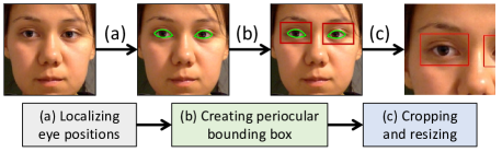
Figure 4. Pipeline of gaze-cropping and resizing: (a) localizing eye positions; (b) creating periocular bounding boxes; and (c) cropping and resizing.

4.5. Frequency Domain Image Processing

Below, we first investigate the impact of the input shape on the time complexity of the CNN, followed by the details of the proposed frequency domain image processing.

4.5.1. Rationale

The time complexity of a convolutional layer is influenced by its FLOPs, memory consumption, and number of parameters (yao2018fastdeepiot, ). For a given CNN with a stack of convolutional layers, the FLOPs of the $l$-th convolutional layer, denoted as $F_{\_}l(I)$, can be calculate by (he2015convolutional, ):

(6) $$F_{\_}l(I)=n_{\_}{l-1}\cdot s_{\_}l^{2}\cdot n_{\_}l\cdot m_{\_}l^{2},$$

where $I$ is the original data input, $n_{\_}{l-1}$ is the number of input channels of the $l$-th convolutional layer, $s_{\_}l^{2}$ is the spatial size of the filter, i.e., the size of the first two dimensions, $n_{\_}l$ is the number of filters in the $l$-th convolutional layer, and $m_{\_}l^{2}$ is the spatial size of the output feature map. We also use $O_{\_}l(I)=n_{\_}l\cdot m_{\_}l^{2}$ to denote the output size of the $l$-th convolutional layer.

Similarly, the memory consumption of the $l$-th convolutional layer, denoted as $M_{\_}l(I)$, can be calculated by (yao2018fastdeepiot, ):

(7) $$M_{\_}l(I)=m_{\_}{l-1}^{2}\cdot n_{\_}{l-1}+m_{\_}{l}^{2}\cdot n_{\_}{l}+m_{\_}{l}^{2}\cdot s_{\_}l^{2}\cdot n_{\_}{l-1},$$

where $m_{\_}{l-1}^{2}$ is the spatial size of the input feature map.

As a toy example to motivate our design, we consider two network inputs with the same size but different shapes: input $I_{\_}1$ has the shape of $224\times 224\times 3$, while input $I_{\_}2$ has the shape of $28\times 28\times 192$. The spatial size of $I_{\_}1$ is 64 times of that of $I_{\_}2$, i.e., $(224\cdot 224)/(28\cdot 28)=64$. We assume the first convolutional layer of the CNN has 64 filters and the filter spatial size is 3$\times$3. We also assume that the stride of the convolutional layer is one and padding is used.

For the first convolutional layer, its output shape is $224\times 224\times 64$ and $28\times 28\times 64$, for $I_{\_}1$ and $I_{\_}2$, respectively. Based on Equation (6), $I_{\_}1$ and $I_{\_}2$ lead to the same FLOPs for the first convolutional layer:

(8) $$F_{\_}1(I_{\_}1)=3\cdot 3^{2}\cdot 64\cdot 224^{2}=F_{\_}1(I_{\_}2)=192\cdot 3^{2}\cdot 64\cdot 28^{2}.$$

Based on Equation (7), we can also calculate the corresponding memory consumption as:

(9) $$M_{\_}1(I_{\_}1)=224^{2}\cdot 3+224^{2}\cdot 64+224^{2}\cdot 3^{2}\cdot 3=4,716,544.$$

(10) $$M_{\_}1(I_{\_}2)=28^{2}\cdot 192+28^{2}\cdot 64+28^{2}\cdot 3^{2}\cdot 192=1,555,456.$$

Thus, for the first convolutional layer, $I_{\_}1$ and $I_{\_}2$ result in the same FLOPs, but $M_{\_}1(I_{\_}1)$ is more than three times of $M_{\_}1(I_{\_}2)$.

For the $l$-th convolutional layer when $l\geq 2$, we can further rewrite Equations (6) and (7) as:

(11) $$F_{\_}l(I)=n_{\_}{l-1}\cdot s_{\_}l^{2}\cdot O_{\_}{l}(I),$$

(12) $$M_{\_}l(I)=O_{\_}{l-1}(I)+O_{\_}{l}(I)\left(1+s_{\_}l^{2}\cdot(\frac{n_{\_}{l-1}}{n_{\_}l})\right).$$

Moreover, from the second convolutional layer, the values of $s_{\_}l$, $n_{\_}{l-1}$, and $n_{\_}l$ are independent from the original network input $I$. Thus, as shown in Equations (11) and (12), we can consider both $F_{\_}l(I)$ and $M_{\_}l(I)$ as functions of $O_{\_}{l}(I)$. Finally, given $O_{\_}1(I_{\_}1)$ is 64 times of $O_{\_}1(I_{\_}2)$ in our example, we have $F_{\_}l(I_{\_}1)\approx 64\cdot F_{\_}l(I_{\_}2)$ and $M_{\_}l(I_{\_}1)\approx 64\cdot M_{\_}l(I_{\_}2)$, for any convolutional layer with $l\geq 2$. Note that the magic number 64 comes from the ratio of the spatial size of the inputs. Based on the above analysis, we can draw a conclusion that reducing the spatial size of the CNN input can dramatically reduce its FLOPs and memory consumption, and thus reduces the time complexity. In addition, if we can also reduce the number of channels of input, e.g., from $28\times 28\times 192$ to $28\times 28\times 12$, both FLOPs and memory consumption can be further reduced.

4.5.2. Design

Apparently, simply reshaping and compressing the original RGB input will destroy the perceptual information it contains. To resolve this challenge, we leverage the discrete cosine transform (DCT) to convert the inputs from the RGB domain to the frequency domain, and leverage the frequency domain DCT coefficients as the inputs for gaze estimation. This enables us to reshape the original input without losing the essential perceptual information. Moreover, the spectral compaction (rao2014discrete, ) property of the DCT transformation tells us that most of the critical content-defining information of the image is concentrated in the low-end of the frequency spectrum, whereas signals in the high-frequency end are mostly trivial and are associated with noise (wallace1991jpeg, ). Therefore, we can leverage this property to significantly compact the essential perceptual information in the facial image by a few DCT coefficients in the low-frequency domain. In fact, this is a well-known property that has been widely exploited by data compression techniques, such as the JPEG compression standard (pennebaker1992jpeg, ), where the quantization process rounds off most of the high frequency components during image compression (chen1984scene, ). Our method is orthogonal to existing efforts in model compression (cheng2018model, ) and data offloading (yao2020deep, ), and can be used in parallel to further reduce the system latency.

The pipeline of the proposed frequency domain image processing is shown in Figure 5. It takes an RGB facial image with the shape $W\times H\times 3$ as the input, where $W$ and $H$ denotes the width and height, respectively. First, we apply color space transformation to convert the input image from the RGB color space to the YCbCr color space, which results in three components: one luma component (Y), representing the brightness, and two chroma components (Cb and Cr), representing the chrominance of the image. As shown in Figure 5, the spatial resolution of the Cb and Cr components is reduced by a factor of two. This is because human visual system is more sensitive to fine-grained brightness details, but less susceptible to the hue and color details of an image. Thus, the two chroma components can be compressed (pennebaker1992jpeg, ; zhang2021intelligent, ).

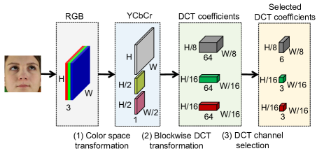
Figure 5. The pipeline of the proposed frequency domain image processing. The input RGB facial image is (1) first converted to the YCbCr color space with the chroma components downsampled. (2) Then, we apply the blockwise DCT transformation on the three components to obtain the corresponding DCT coefficients matrix. (3) Finally, we perform the DCT channel selection to retain only the essential DCT coefficients as the input for gaze estimation.

After the color space transformation, each of the Y, Cb, and Cr components is partitioned into multiple $8\times 8$ rectangular nonoverlapping blocks. Then, we apply the blockwise discrete cosine transform (DCT) to obtain the frequency domain representations, i.e., the DCT coefficients. Specifically, given a block $\mathbf{B}\in\mathbb{R}^{8\times 8}$, the corresponding DCT coefficients are denoted by matrix $\mathcal{B}\in\mathbb{R}^{8\times 8}$, whose element $\mathcal{B}_{\_}{i,j}$ is obtained by (ahmed1974discrete, ):

(13) $$\mathcal{B}_{\_}{i,j}=s(i)s(j)\sum_{\_}{n=0}^{7}\sum_{\_}{m=0}^{7}\mathbf{B}_{\_}{n,m}\cos\Big{[}\frac{\pi}{8}\Big{(}n+\frac{1}{2}\Big{)}i\Big{]}\cos\Big{[}\frac{\pi}{8}\Big{(}m+\frac{1}{2}\Big{)}j\Big{]},$$

where $\mathbf{B}_{\_}{n,m}$ is the pixel value at coordinate $(n,m)$; integers ${0\leq i\leq 7}$ and ${0\leq j\leq 7}$ represent the horizontal and the vertical frequency, respectively; $s(i)$ is a normalization factor to make the transformation orthonormal, for which $s(i)=(\frac{1}{8})^{0.5}$ if $i=0$ and $s(i)=0.5$ otherwise. In sum, each block $\mathbf{B}$ is represented in the frequency domain by a weighted combination of 64 orthogonal sinusoids, where $\mathcal{B}_{\_}{i,j}$ is DCT coefficient that indicates the spectral energy. After the DCT transformation, we scan each of the $8\times 8$ DCT coefficients matrices in a zigzag order starting from the top-left corner and subsequently convert it to a $1\times 64$ vector. As shown in Figure 5, the outputs of the DCT transformation are three coefficients matrices, with the shape of $\frac{W}{8}\times\frac{H}{8}\times 64$, $\frac{W}{16}\times\frac{H}{16}\times 64$, and $\frac{W}{16}\times\frac{H}{16}\times 64$, for the Y, Cb, and Cr components, respectively.

Finally, taking advantage of the spectral compaction property of DCT, we perform DCT channel selection to further compress the DCT coefficients matrix and retain a small subset of it as the data input for the gaze estimation. As shown in Figure 5, instead of maintaining all the 64 channels, we only keep the lowest six, three, and three channels for the Y, Cb, and Cr components, respectively, and prune the other high-frequency channels. Taking an RGB image with the size of $224\times 224\times 3$ as the input, the frequency domain image processing outputs the selected DCT coefficients matrix of Y, Cb, and Cr, with the shape of $28\times 28\times 6$, $14\times 14\times 3$ and $14\times 14\times 3$, respectively. The selected DCT coefficients matrices are then fed into the gaze embedding network for representation learning.

4.6. Gaze Embedding Network

Figure 6 shows the architecture of the gaze embedding network, which follows a ResNet-18 (he2016deep, ) based design. Since the DCT coefficients matrix of the Y component has a larger spatial size than that of the Cb/Cr components, we cannot feed the three DCT coefficients matrices directly to a conventional CNN. A naive solution is to downsample the input of Y component or upsample the input of the Cb/Cr components to align the spatial sizes. However, it will lead to information loss or a higher time complexity. Thus, we have to design the CNN network carefully so that it can take the three matrices with different sizes as inputs. Specifically, we adopt the late concatenate (gueguen2018faster, ) , which has approved to ensure better learning performance. As depicted in Figure 6, the DCT coefficients matrix of the Y component is first passed through two residual blocks consist of four convolutional layers, whose output shape is $14\times 14\times 128$. In parallel, the DCT coefficients matrices of Cb/Cr are first concatenated, followed by fed into a single convolutional layer, for which the output shape is $14\times 14\times 128$. Then, the outputs of two parallel paths are concatenated as they have the same spatial size. After that, the joint representations are fed into two residual blocks which correspond to block conv5 in the original ResNet-18 design. The final output of the gaze embedding network is the gaze representations, which is a vector of 512 features. In our design, we apply batch normalization (BN) (ioffe2015batch, ) right after each convolution and before activation, and also adopt BN after the input layer to ensure better performance. Note that the architecture shown in Figure 6 contains eight convolutional layers in the deepest path, which is eight layers shallower than the original ResNet-18. We adopt the current design after balancing the gaze estimation accuracy and system latency. We provide a detailed investigation on this trade-off in Section 5.3.5.

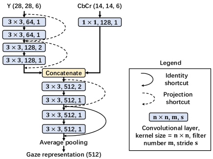
Figure 6. The architecture of the gaze embedding network.

5. Evaluation

5.1. Datasets

We consider two public gaze estimation datasets in our evaluation.

• ETH-XGaze (zhang2020eth, ) is the state-of-the-art appearance-based gaze estimation dataset, which originally consists of one training and two testing sets. The images in the training set are released with gaze labels, whereas the labels for the testing sets are not available, i.e., testing results can only be evaluated via the project leaderboard (ETHXGazeLEADERBOARD, ). Thus, we only take the original training set of ETH-XGaze for our evaluation, which consists of 80 subjects with diverse genders, ages, and ethnicity backgrounds. Some of the subjects wore contact lenses or eye glasses during the data collection. We consider the application scenario of using smartphone front-camera and web-camera for gaze estimation, and select images with the front-facing head pose. We further split the selected data into two parts: a pre-training set comprised of 70 subjects, and a calibration set consists of the remaining 10 subjects. Each subject has 380 to 600 images. In total, the pre-training set has 36,731 images and the calibration set has 4,718 images. The resolution of image is 448 $\times$ 448.

• MPIIFaceGaze (zhang2017mpiigaze, ) is collected from 15 subjects. Each subject has 3,000 images with diverse head poses and illumination conditions. We take the images collected from the first ten subjects to form the pre-training set, and that from the remaining five subjects to form the calibration set, which results in a size of 30,000 and 15,000 images for the pre-training and calibration set, respectively.

Data preparation. For both datasets, the pre-training set is used to pre-train the gaze embedding network, which is conducted in either a supervised or unsupervised way, depending on the representation learning method considered. For each subject in the calibration set, the subject’s data is further divided into three parts: (1) a fine-tuning set for fine-tuning the pre-trained gaze embedding network and the gaze estimator in a subject-dependent manner; (2) a validation set for network validation; and (3) a testing set to evaluate the gaze estimation performance after the fine-tuning. Specifically, for each subject in the calibration set (ten subjects for the ETH-XGaze and five subjects for the MPIIFaceGaze), we randomly sample 75 images to form the fine-tuning set, 25 images to form the validation set, and use the remaining images to form the testing set. For each subject, we have 280 to 500 testing images for the ETH-XGaze and 2,900 testing images for the MPIIFaceGaze. In Section 5.3.4, we study how the fine-tuning set size affects the gaze estimation performance.

5.2. Methodology

5.2.1. Methods in comparison

We compare the gaze estimation performance of different supervised and self-supervised methods.

• FreeGaze: the proposed self-supervised method. Specifically, we first pre-train the gaze embedding network by following the frequency domain contrastive gaze representation learning introduced in Section 4. Then, we fine-tune the gaze embedding network and the randomly initialized gaze estimator using the images in the fine-tuning set.

• FreeGaze-Mix: a variant of FreeGaze. Differently, during the self-supervised learning stage, images in the minibatch are randomly sampled from the whole pre-training set, without using the subject-specific negative pair sampling strategy introduced in Section 4.3.

We also consider three baselines that take RGB images as the inputs:

• RGB-Supervised: we leverage the pre-training set to pre-train the gaze embedding network and the gaze estimator in a supervised manner, i.e., 37K labeled images for ETH-XGaze and 30K labeled images for MPIIFaceGaze. We further fine-tune them during the calibration stage.

• RGB-Random: we randomly initialize the parameters of the gaze embedding network and the gaze estimator without pre-training. We only fine-tune them during the calibration stage.

• RGB-SimCLR: we leverage the state-of-the-art contrastive learning framework, i.e., SimCLR (chen2020simple, ), to pre-train the gaze embedding network. Specifically, we adopt the data augmentation operators introduced in SimCLR, i.e., random cropping followed by image resizing and random color distortion, and apply them sequentially on the RGB images to generate positive and negative image pairs. Moreover, in self-supervised learning stage, images in the minibatch are randomly sampled from the whole pre-training set. The gaze estimator is randomly initialized. Both networks are then fine-tuned during the calibration stage.

Lastly, we consider DCT-Supervised and DCT-SimCLR. Specifically, DCT-Supervised leverages the DCT coefficients matrices generated by the frequency domain signal processing as the inputs for both pre-training and calibration. For DCT-SimCLR, we obtain the DCT coefficients of the RGB images that are augmented by the data augmentation methods in SimCLR. Different from FreeGaze, DCT-SimCLR adopts neither the subject-specific negative pair sampling strategy nor the stochastic gaze-specific data augmentation.

5.2.2. Implementation

We implement all the methods with Python and TensorFlow 2.0. For RGB-based methods, the gaze embedding network follows the design of ResNet-18 (he2016deep, ) (without the dense layers). For DCT-based methods, the gaze embedding network follows the structure shown in Figure 6. We use the Adam optimizer (kingma2014adam, ) during the training. In the pre-training stage, all methods use the same batch size of 128. The learning rate for FreeGaze, FreeGaze-Mix, RGB-SimCLR, and DCT-SimCLR is 0.01; the learning rate for RGB-Supervised and DCT-Supervised is 0.001. For all methods, the resolution of the input images is $224\times 224$. In the calibration stage, the learning rate for RGB-Supervised, RGB-SimCLR, and RGB-Random is 0.00025 with a decay of 0.0005. The learning rate for FreeGaze, FreeGaze-Mix, DCT-SimCLR is 0.002. The learning rate for DCT-Supervised is 0.0005 with a decay of 0.0005. Note that, for the four DCT-based methods, we use images with the resolution of $448\times 448$ to fine-tune the network, which improves estimation accuracy. We do not apply this to the three RGB-based methods, as it leads to high calibration latency, i.e., 10 to 21 minutes as measured in Section 5.4.1, which makes it an impractical design choice. For fair comparison, all methods use the same pre-training set for either unsupervised or supervised pre-training. In the calibration stage, we randomly sample the fine-tuning and the validation sets for six times, and all methods use the same sets of data for fine-tuning and testing. We report the averaged result as the final accuracy.

5.3. Performance in Gaze Estimation

5.3.1. Performance metrics

As shown in Figure 7, we use the angular error $\theta$ (in degree) and the distance error $\epsilon$ (in cm) as the performance metrics. Specifically, $\theta$ represents the angle between the estimated and actual gaze vectors; while $\epsilon$ measures the euclidean distance between the estimated and actual gaze points on the screen plane, given the viewing distance $d$.

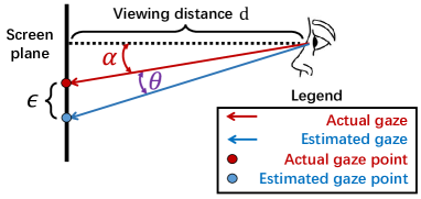
Figure 7. Illustration of the performance metrics used for gaze estimation: (1) the angular error, $\theta$, represents the angle (in degree) between the estimated and the actual gazes; the distance error, $\epsilon$, represents the euclidean distance (in cm) between the estimated and the actual gaze points on the screen plane, given a viewing distance $d$.

5.3.2. Comparison with RGB-based methods

We compare the proposed FreeGaze with the RGB-based methods, i.e., RGB-Supervised, RGB-Random, and RGB-SimCLR. Figure 8 shows the angular error on each subject in the testing set. The averaged angular errors are given in Table 1. We make the following observations.

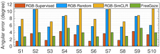
(a) ETH-XGaze

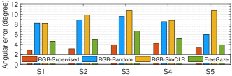
(b) MPIIFaceGaze

Figure 8. Angular error of the examined methods on (a) ETH-XGaze and (b) MPIIFaceGaze. FreeGaze achieves similar performance with RGB-Supervised, and outperforms RGB-Random and RGB-SimCLR by a large margin in all cases.

First, RGB-Supervised, which leverages 37K and 30K labeled RGB images to train the gaze embedding network and the gaze estimator, achieves the lowest angular error in all examined cases. By contrast, without the help from the supervised pre-training, the angular error of RGB-Random is significantly higher.

Table 1. Averaged angular errors (mean$\pm$std) on ETH-XGaze and MPIIFaceGaze.

	ETH-XGaze	MPIIFaceGaze
RGB-Supervised	1.81${}^{\circ}\pm$0.75∘	3.50${}^{\circ}\pm$0.56∘
RGB-Random	7.67${}^{\circ}\pm$2.30∘	8.24${}^{\circ}\pm$1.35∘
RGB-SimCLR	8.38${}^{\circ}\pm$1.63∘	9.65${}^{\circ}\pm$1.12∘
FreeGaze	2.95${}^{\circ}\pm$0.51∘	5.07${}^{\circ}\pm$1.03∘

Second, RGB-SimCLR has the highest angular error. This indicates that conventional SimCLR cannot be used directly for gaze estimation, and the gaze embedding network has poor representation learning performance when training by SimCLR. There are two reasons for this result. First, SimCLR performs random image cropping when generating the positive image pairs (chen2020simple, ), which potentially removes the gaze-related features, and thus, adding confusions to the gaze embedding network during the representation learning. Second, when forming the minibatch, SimCLR randomly samples images from the whole pre-training set to generate negative pairs, and considers images from different subjects as negative pairs. However, as discussed in Section 3.1 and demonstrated in Figure 1,contrastive learning ensures the representations of visually similar images, i.e., images of the same subject, are close to each other in the latent space (hadsell2006dimensionality, ), while the representations of visually distinct images are as separated as possible (ye2019unsupervised, ). Thus, when images of different subjects are considered as negative pairs, the gaze embedding network tends to learn representations that are useful for subject classification, instead of gaze estimation. These two factors make SimCLR ineffective for the aimed purpose.

Lastly, the proposed FreeGaze achieves similar performance with RGB-Supervised, and out-performs both RGB-Random and RGB-SimCLR by a large margin. The performance gap in angular error between FreeGaze and RGB-Supervised is 1.14^∘ and 1.57^∘ on ETH-XGaze and MPIIFaceGaze, respectively.

Performance in different application scenarios. As shown in Figure 7, we also use the distance error $\epsilon$ as the performance metric. This allows us to quantify the gaze estimation performance with the consideration of typical application scenarios, e.g., eye tracking using front-facing camera on smartphone and desktop computer. Given the angular error $\theta$, we can calculate $\epsilon$ by:

(14) $$\epsilon=d\times\big{(}\tan(\alpha+\theta)-\tan(\alpha)\big{)},$$

where $d$ is the viewing distance and $\alpha$ is the actual gaze angle. Then, taking the averaged angular errors reported in Table 1, we calculate the corresponding distance error $\epsilon$ as a function of $d$ and $\alpha$. Specifically, we set $d$ equals 30cm and 50cm, respectively, to represent the typical viewing distance when a subject is using smartphone (boccardo2021viewing, ; long2017viewing, ) and desktop computer (rempel2007effects, ), respectively. The actual gaze angle $\alpha$ changes from 0^∘ to 30^∘, which is the range of the standard viewing angle when interacting with digital visual displays (johnson1997hci, ; greeson1996international, ). The averaged distance errors of the four methods are shown in Figure 9. FreeGaze outperforms RGB-Random and RGB-SimCLR by a large margin, and achieves acceptable performance when comparing with RGB-Supervised. Specifically, in the smartphone viewing scenario, i.e., $d=30$cm, the averaged performance gap (in distance error) between FreeGaze and RGB-Supervised is only 0.45cm and 0.64cm, on ETH-XGaze and MPIIFaceGaze, respectively. In the desktop viewing scenario, i.e., $d=50$cm, the averaged performance gap increases slightly to 1.13cm and 1.59cm, on ETH-XGaze and MPIIFaceGaze, respectively.

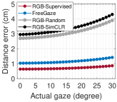
(a) ETH-XGaze ($d=30cm$)

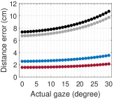
(b) ETH-XGaze ($d=50cm$)

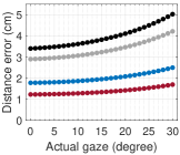
(c) MPIIFaceGaze ($d=30cm$)

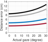
(d) MPIIFaceGaze ($d=50cm$)

Figure 9. Distance error $\epsilon$ as a function of the viewing distance $d$ and the actual gaze angle $\alpha$.

5.3.3. Comparison with DCT-based methods

We also compare the gaze estimation performance of the four DCT-based methods. The results are shown in Figure 10.

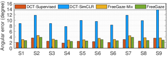
(a) ETH-XGaze

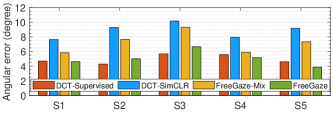
(b) MPIIFaceGaze

Figure 10. Angular error of the DCT-based methods on (a) ETH-XGaze and (b) MPIIFaceGaze dataset.

Overall, on ETH-XGaze the angular error averaged on the ten subjects is 2.61${}^{\circ}\pm$0.64^∘, 10.11${}^{\circ}\pm$2.00^∘, 3.53${}^{\circ}\pm$0.59^∘, and 2.95${}^{\circ}\pm$0.51^∘, for DCT-Supervised, DCT-SimCLR, FreeGaze-Mix, and FreeGaze, respectively. Similarly, on MPIIFaceGaze the angular error averaged on the five subjects is 4.97${}^{\circ}\pm$0.62^∘, 8.84${}^{\circ}\pm$1.04^∘, 7.20${}^{\circ}\pm$1.44^∘, and 5.07${}^{\circ}\pm$1.03^∘, for the four methods, respectively. We make the following additional observations.

DCT-Supervised achieves the lowest angular error, as it leverages labeled DCT coefficients for supervised training. The proposed FreeGaze achieves the lowest angular error amongst the three unsupervised methods. Specifically, FreeGaze outperforms FreeGaze-Mix by 0.56^∘ and 2.14^∘ on average, for ETH-XGaze and MPIIFaceGaze, respectively. This improvement comes from the adoption of the subject-specific negative pair sampling strategy introduced in Section 4.3. By contrast, FreeGaze-Mix leverages the conventional minibatch sampling strategy introduced in SimCLR, which treats images from different subjects as negative pairs. Nevertheless, FreeGaze-Mix still outperforms DCT-SimCLR by a large margin: 6.58^∘ and 1.64^∘ on average for the two datasets, respectively. This result further indicates that the random image cropping used by SimCLR adds confusions to the gaze embedding network during the representation learning, and leads to poor estimation performance. By contrast, using of the gaze-specific data augmentation (introduced in Section 4.4), both FreeGaze and FreeGaze-Mix can maintain the gaze-related features and ensure good representation learning capability. Lastly, the performance gap between FreeGaze and DCT-Supervised is 0.36^∘ and 0.09^∘ on average for the two datasets, which demonstrates the effectiveness of the proposed unsupervised learning framework for learning gaze representations in the frequency domain.

5.3.4. Impact of fine-tuning set size

We also investigate the impact of the fine-tuning set size on the gaze estimation performance. For both ETH-XGaze and MPIIFaceGaze, we use different numbers of labeled images for the calibration. The results are shown in Figure 11. The angular errors for all examined methods decrease with the increase of the fine-tuning set size. The accuracy gain is more prominent for RGB-Random, and less significant for RGB-Supervised. With 125 samples for the fine-tuning, the performance gain between FreeGaze and RGB-Supervised can decrease to 0.99^∘ and 1.07^∘ on ETH-XGaze and MPIIFaceGaze, respectively.

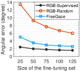
(a) ETH-XGaze

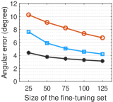
(b) MPIIFaceGaze

Figure 11. Impact of the fine-tuning set size on the gaze estimation performance: (a) ETH-XGaze and (b) MPIIFaceGaze.

5.3.5. Impact of model size

To investigate the impact of model size on the gaze estimation performance, we consider two different designs of the gaze embedding network. We denote the original architecture shown in Figure 6 as FreeGaze-8CNN, indicating that it contains eight convolutional layers in the deepest path. We further design FreeGaze-12CNN, for which the DCT coefficients matrix of the Y component is passed through four residual blocks, which correspond to blocks conv2 and conv3 in the original ResNet-18. This makes FreeGaze-12CNN four-layers deeper than FreeGaze-8CNN. Table 2 compares the performance of the two designs on ETH-XGaze and MPIIFaceGaze datasets. Overall, they exhibit similar performance on ETH-XGaze, while FreeGaze-12CNN achieves a modest 0.6^∘ improvement over FreeGaze-8CNN on MPIIFaceGaze.

Table 2. Averaged angular errors (mean$\pm$std) on ETH-XGaze and MPIIFaceGaze with different model sizes.

	ETH-XGaze	MPIIFaceGaze
FreeGaze-8CNN	2.95${}^{\circ}\pm$0.51∘	5.07${}^{\circ}\pm$1.03∘
FreeGaze-12CNN	2.98${}^{\circ}\pm$0.59∘	4.46${}^{\circ}\pm$1.02∘

5.4. Evaluation of System Latency

Below, we profile the system latency in calibration and inference. We consider three different designs of the gaze embedding network: (1) RGB-ResNet18, which leverages the ResNet18-based network architecture. This design is adopted by the three RGB-based baseline methods introduced in Section 5.2; (2) FreeGaze-8CNN; and (3) FreeGaze-12CNN. We consider RGB images with resolutions $224\times 224$ and $448\times 448$ as the original inputs. Table 3 shows the FLOPs and the number of parameters for the three system designs, given different input image resolutions. We evaluate the system latency on a desktop installed with an Intel i7-11700KF CPU and a NVIDIA GeForce RTX 3080Ti GPU, as well as a server equipped with a NVIDIA GeForce RTX 2080Ti GPU.

Table 3. The FLOPs (in the unit of $10^{9}$) and the number of parameters of the three network designs given different input image resolutions.

	FLOPs		# parameters
	224*224	448*448
RGB-ResNet18	1.82	7.25	11,190,912
FreeGaze-8CNN	0.49	1.96	8,675,824
FreeGaze-12CNN	0.61	2.42	9,046,380

5.4.1. Calibration Latency

We first measure the calibration latency. Specifically, we train the gaze embedding network and the gaze estimator for 1,500 epochs. The size of the fine-tuning and validation sets is 75 and 25, respectively. We repeat this procedure for five times, and report the averaged latency. The results are shown in Table 4. Given different settings, FreeGaze-8CNN achieves 3.33 to 6.81 times speedup over the RGB-ResNet18 based design. Clearly, one can use a smaller fine-tuning set and a smaller training epoch to accelerate the calibration process. However, this is at the cost of sacrificing the estimation accuracy, i.e., smaller fine-tuning sets lead to higher angular error and smaller training epoch leads to network underfitting.

Table 4. Calibration latency (in min) for the three network designs with different input image resolutions. Overall, FreeGaze-8CNN achieves 3.33 to 6.81 times speedup over the RGB-ResNet18 based design.

	224$\times$224		448$\times$448
	2080Ti	3080Ti	2080Ti	3080Ti
RGB-ResNet18	6.6	3.0	21.1	10.2
FreeGaze-8CNN	1.7	0.9	3.1	1.8
FreeGaze-12CNN	2.1	1.2	4.0	2.3

5.4.2. Inference Latency

To measure the inference latency, we randomly sample an image from the testing set for gaze estimation. The inference process involves the gaze representations extraction performed by the gaze embedding network and the gaze estimation performed by the gaze estimator. We repeat the measurement for 5,000 times, and report the averaged latency. For DCT-based methods, we also measure the time required by the frequency domain image processing module, which takes 0.1ms and 0.8ms for image with resolution 224$\times$224 and 448$\times$448, respectively. The results are shown in Table 5. Given different settings, FreeGaze-8CNN achieves 1.59 to 1.67 times speedup over the RGB-ResNet18 based design.

Table 5. Inference latency (in ms) for the three network designs with different input image resolutions. Overall, FreeGaze-8CNN achieves 1.59 to 1.67 times speedup over the RGB-ResNet18 based design.

	224$\times$224		448$\times$448
	2080Ti	3080Ti	2080Ti	3080Ti
RGB-ResNet18	27.0	14.9	27.0	15.6
FreeGaze-8CNN	17.0	8.9	17.0	9.6
FreeGaze-12CNN	21.0	11.8	22.0	12.0

Discussion. The reductions in calibration and inference latency (reported in Tables 4 and 5) are not proportional to the FLOPs (listed in Table 3). For instance, when the input image is with the resolution of 448$\times$448, the FLOPs of RGB-ResNet18 is 3.7 times of that of FreeGaze-8CNN, but the calibration and inference latency is 5.7 and 1.6 times, respectively. This is because using FLOPs alone cannot precisely estimates system latency on modern computation hardware, e.g., TPUs and GPUs. The system latency is often bounded by memory access costs, and there exists different levels of optimization on modern matrix multiplication units (bello2021revisiting, ; jouppi2017datacenter, ). For instance, a ResNet-RS model with 1.8 times more FLOPs than EfficientNet-B6 is 2.7 times faster on a TPUv3 hardware accelerator (bello2021revisiting, ). Thus, the actual runtime system latency is affected by the computer-to-memory-ratio, the operational intensity affects, and the other optimizations on the computation hardware.

5.4.3. Overall System Performance Comparison

Lastly, we trade-off different design choices and perform an overall performance comparison. Specifically, for FreeGaze-8CNN and FreeGaze-12CNN, we trade-off system latency for estimation accuracy, and use images with the resolution of $448\times 448$ to fine-tune the network. We do not apply this to RGB-ResNet18, as it results in 10 to 21 minutes latency for the on the fly system calibration and makes it an impractical design choice. Figure 12 shows the overall performance comparison when trading-off gaze estimation accuracy (angular error) with calibration or inference latency. The results are based on the profiling on a RTX 2080Ti GPU. For the interest of space, we omit the comparison on RTX 3080Ti and the MPIIFaceGaze dataset as they exhibit similar trends. When comparing with RGB-Supervised, FreeGaze-8CNN achieves 2.13 and 1.59 times speedup in calibration and inference, while sacrificing 1.1^∘ estimation accuracy. Note that the performance gain achieved by RGB-Supervised is also at the cost of labour of intensive gaze data labeling, i.e., 37K labeled images and 30K labeled images for ETH-XGaze and MPIIFaceGaze, respectively. By contrast, FreeGaze-8CNN overcomes the data labeling hurdle and achieves satisfactory gaze estimation performance in an unsupervised way.

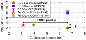
(a) Angular error vs. calibration latency

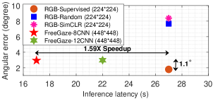
(b) Angular error vs. inference latency

Figure 12. Performance comparison when trading-off estimation accuracy with (a) calibration latency and (b) inference latency. Comparing with RGB-Supervised, FreeGaze-8CNN achieves 2.13 and 1.59 times speedup in calibration and inference, while sacrificing 1.1^∘ estimation accuracy.

6. Conclusion

In this work, we present FreeGaze, a resource-efficient framework that incorporates the frequency domain gaze estimation and the contrastive gaze representation learning for unsupervised gaze estimation. Our evaluation on two gaze estimation datasets demonstrates the validity of FreeGaze. Specifically, FreeGaze achieves comparable gaze estimation accuracy with RGB supervised learning-based approach, and reduces the angular error of existing unsupervised approach by 5.4^∘ and 4.6^∘ on average over the two datasets, respectively. FreeGaze also enables up to 6.81 and 1.67 times speedup in system calibration and gaze estimation, respectively.

References

- (1) D. W. Hansen and Q. Ji, “In the eye of the beholder: A survey of models for eyes and gaze,” IEEE Transactions on Pattern Analysis and Machine Intelligence, vol. 32, no. 3, pp. 478–500, 2009.
- (2) M. K. Eckstein, B. Guerra-Carrillo, A. T. M. Singley, and S. A. Bunge, “Beyond eye gaze: What else can eyetracking reveal about cognition and cognitive development?” Developmental Cognitive Neuroscience, vol. 25, pp. 69–91, 2017.
- (3) E. Shishido, S. Ogawa, S. Miyata, M. Yamamoto, T. Inada, and N. Ozaki, “Application of eye trackers for understanding mental disorders: Cases for schizophrenia and autism spectrum disorder,” Neuropsychopharmacology reports, vol. 39, no. 2, pp. 72–77, 2019.
- (4) H. Duan, G. Zhai, X. Min, Z. Che, Y. Fang, X. Yang, J. Gutiérrez, and P. L. Callet, “A dataset of eye movements for the children with autism spectrum disorder,” in Proceedings of the ACM Multimedia Systems Conference (MMSys), 2019, pp. 255–260.
- (5) S. Berkovsky, R. Taib, I. Koprinska, E. Wang, Y. Zeng, J. Li, and S. Kleitman, “Detecting personality traits using eye-tracking data,” in Proceedings of the ACM Conference on Human Factors in Computing Systems (CHI), 2019, pp. 1–12.
- (6) T. Kosch, M. Hassib, P. W. Woźniak, D. Buschek, and F. Alt, “Your eyes tell: Leveraging smooth pursuit for assessing cognitive workload,” in Proceedings of the ACM Conference on Human Factors in Computing Systems (CHI), 2018, pp. 1–13.
- (7) L. Fridman, B. Reimer, B. Mehler, and W. T. Freeman, “Cognitive load estimation in the wild,” in Proceedings of the ACM Conference on Human Factors in Computing Systems (CHI), 2018, pp. 1–9.
- (8) B. De Haas, A. L. Iakovidis, D. S. Schwarzkopf, and K. R. Gegenfurtner, “Individual differences in visual salience vary along semantic dimensions,” Proceedings of the National Academy of Sciences, vol. 116, no. 24, pp. 11 687–11 692, 2019.
- (9) J. Najemnik and W. S. Geisler, “Optimal eye movement strategies in visual search,” Nature, vol. 434, no. 7031, pp. 387–391, 2005.
- (10) S. Marwecki, A. D. Wilson, E. Ofek, M. Gonzalez Franco, and C. Holz, “Mise-Unseen: Using eye tracking to hide virtual reality scene changes in plain sight,” in Proceedings of the ACM Symposium on User Interface Software and Technology (UIST), 2019, pp. 777–789.
- (11) A. Patney, M. Salvi, J. Kim, A. Kaplanyan, C. Wyman, N. Benty, D. Luebke, and A. Lefohn, “Towards foveated rendering for gaze-tracked virtual reality,” ACM Transactions on Graphics, vol. 35, no. 6, pp. 1–12, 2016.
- (12) J. Kim, Y. Jeong, M. Stengel, K. Akşit, R. Albert, B. Boudaoud, T. Greer, J. Kim, W. Lopes, Z. Majercik et al., “Foveated AR: Dynamically-foveated augmented reality display,” ACM Transactions on Graphics, vol. 38, no. 4, pp. 1–15, 2019.
- (13) N. Valliappan, N. Dai, E. Steinberg, J. He, K. Rogers, V. Ramachandran, P. Xu, M. Shojaeizadeh, L. Guo, K. Kohlhoff et al., “Accelerating eye movement research via accurate and affordable smartphone eye tracking,” Nature Communications, vol. 11, no. 1, pp. 1–12, 2020.
- (14) E. Wood and A. Bulling, “EyeTab: Model-based gaze estimation on unmodified tablet computers,” in Proceedings of the ACM Symposium on Eye Tracking Research and Applications (ETRA), 2014, pp. 207–210.
- (15) Y. Sugano, X. Zhang, and A. Bulling, “AggreGaze: Collective estimation of audience attention on public displays,” in Proceedings of the ACM Annual Symposium on User Interface Software and Technology (UIST), 2016, pp. 821–831.
- (16) Y. Cheng, H. Wang, Y. Bao, and F. Lu, “Appearance-based gaze estimation with deep learning: A review and benchmark,” arXiv preprint arXiv:2104.12668, 2021.
- (17) C. Kelton, J. Ryoo, A. Balasubramanian, and S. R. Das, “Improving user perceived page load times using gaze,” in Proceedings of USENIX Symposium on Networked Systems Design and Implementation (NSDI), 2017, pp. 545–559.
- (18) G. Lan, B. Heit, T. Scargill, and M. Gorlatova, “GazeGraph: graph-based few-shot cognitive context sensing from human visual behavior,” in Proceedings of the ACM Conference on Embedded Networked Sensor Systems (SenSys), 2020, pp. 422–435.
- (19) N. Srivastava, J. Newn, and E. Velloso, “Combining low and mid-level gaze features for desktop activity recognition,” Proceedings of the ACM on Interactive, Mobile, Wearable and Ubiquitous Technologies, vol. 2, no. 4, p. 189, 2018.
- (20) S. Gillet, R. Cumbal, A. Pereira, J. Lopes, O. Engwall, and I. Leite, “Robot gaze can mediate participation imbalance in groups with different skill levels,” in Proceedings of the ACM/IEEE International Conference on Human-Robot Interaction (HRI), 2021, pp. 303–311.
- (21) C. F. Weldon, S. Gillet, R. Cumbal, and I. Leite, “Exploring non-verbal gaze behavior in groups mediated by an adaptive robot,” in Proceedings of the ACM/IEEE International Conference on Human-Robot Interaction (HRI), 2021, pp. 357–361.
- (22) M. Kassner, W. Patera, and A. Bulling, “Pupil: an open source platform for pervasive eye tracking and mobile gaze-based interaction,” in Proceedings of the ACM International Joint Conference on Pervasive and Ubiquitous Computing (UbiComp), 2014, pp. 1151–1160.
- (23) X. Zhang, S. Park, T. Beeler, D. Bradley, S. Tang, and O. Hilliges, “ETH-XGaze: A large scale dataset for gaze estimation under extreme head pose and gaze variation,” in Proceedings of European Conference on Computer Vision (ECCV), 2020, pp. 365–381.
- (24) K. Krafka, A. Khosla, P. Kellnhofer, H. Kannan, S. Bhandarkar, W. Matusik, and A. Torralba, “Eye tracking for everyone,” in Proceedings of the IEEE Conference on Computer Vision and Pattern Recognition (CVPR), 2016, pp. 2176–2184.
- (25) X. Zhang, M. X. Huang, Y. Sugano, and A. Bulling, “Training person-specific gaze estimators from user interactions with multiple devices,” in Proceedings of the ACM Conference on Human Factors in Computing Systems (CHI), 2018, pp. 1–12.
- (26) X. Zhang, Y. Sugano, M. Fritz, and A. Bulling, “MPIIGaze: Real-world dataset and deep appearance-based gaze estimation,” IEEE Transactions on Pattern Analysis and Machine Intelligence, vol. 41, no. 1, pp. 162–175, 2019.
- (27) S. Huynh, R. K. Balan, and J. Ko, “iMon: Appearance-based gaze tracking system on mobile devices,” Proceedings of the ACM on Interactive, Mobile, Wearable and Ubiquitous Technologies, vol. 5, no. 4, pp. 1–26, 2021.
- (28) P. Kellnhofer, A. Recasens, S. Stent, W. Matusik, and A. Torralba, “Gaze360: Physically unconstrained gaze estimation in the wild,” in Proceedings of the IEEE/CVF International Conference on Computer Vision (ICCV), 2019, pp. 6912–6921.
- (29) A. Newman, B. McNamara, C. Fosco, Y. B. Zhang, P. Sukhum, M. Tancik, N. W. Kim, and Z. Bylinskii, “TurkEyes: A web-based toolbox for crowdsourcing attention data,” in Proceedings of the ACM Conference on Human Factors in Computing Systems (CHI), 2020, pp. 1–13.
- (30) “The facebook OpenEDS challenge,” https://research.facebook.com/openeds-challenge/.
- (31) Y. Sugano and A. Bulling, “Self-calibrating head-mounted eye trackers using egocentric visual saliency,” in Proceedings of the Annual ACM Symposium on User Interface Software & Technology (UIST), 2015, pp. 363–372.
- (32) A. Lanata, G. Valenza, A. Greco, and E. P. Scilingo, “Robust head mounted wearable eye tracking system for dynamical calibration,” Journal of Eye Movement Research, vol. 8, no. 5, 2015.
- (33) E. Lindén, J. Sjostrand, and A. Proutiere, “Learning to personalize in appearance-based gaze tracking,” in Proceedings of the IEEE/CVF International Conference on Computer Vision (ICCV), 2019, pp. 1–9.
- (34) “Performing a calibration and validation in Pro Lab,” https://www.tobiipro.com/learn-and-support/learn/steps-in-an-eye-tracking-study/run/performing-a-calibration-and-validation-in-pro-lab/.
- (35) “Calibration process for pupil Labs eye tracker,” https://docs.pupil-labs.com/core/software/pupil-capture/#calibration.
- (36) “Calibration process for VIVO Pro VR headset,” https://developer.vive.com/eu/support/sdk/category_howto/how-to-calibrate-eye-tracking.html.
- (37) R. Albert, A. Patney, D. Luebke, and J. Kim, “Latency requirements for foveated rendering in virtual reality,” ACM Transactions on Applied Perception, vol. 14, no. 4, pp. 1–13, 2017.
- (38) M. L. Mele and S. Federici, “Gaze and eye-tracking solutions for psychological research,” Cognitive Processing, vol. 13, no. 1, pp. 261–265, 2012.
- (39) K. R. Rao and P. Yip, Discrete cosine transform: algorithms, advantages, applications. Academic press, 2014.
- (40) G. K. Wallace, “The JPEG still picture compression standard,” Communications of the ACM, vol. 34, no. 4, pp. 30–44, 1991.
- (41) T. Chen, S. Kornblith, M. Norouzi, and G. Hinton, “A simple framework for contrastive learning of visual representations,” in Proceedings of International Conference on Machine Learning (ICML), 2020, pp. 1597–1607.
- (42) A. Dosovitskiy, J. T. Springenberg, M. Riedmiller, and T. Brox, “Discriminative unsupervised feature learning with convolutional neural networks,” Advances in Neural Information Processing Systems, vol. 27, 2014.
- (43) E. Xie, J. Ding, W. Wang, X. Zhan, H. Xu, P. Sun, Z. Li, and P. Luo, “DetCo: Unsupervised contrastive learning for object detection,” in Proceedings of the IEEE/CVF International Conference on Computer Vision (ICCV), 2021, pp. 8392–8401.
- (44) A. Nakazawa and C. Nitschke, “Point of gaze estimation through corneal surface reflection in an active illumination environment,” in Proceedings of the European Conference on Computer Vision (ECCV), 2012, pp. 159–172.
- (45) E. D. Guestrin and M. Eizenman, “General theory of remote gaze estimation using the pupil center and corneal reflections,” IEEE Transactions on Biomedical Engineering, vol. 53, no. 6, pp. 1124–1133, 2006.
- (46) X. Zhang, Y. Sugano, M. Fritz, and A. Bulling, “Appearance-based gaze estimation in the wild,” in Proceedings of the IEEE Conference on Computer Vision and Pattern Recognition (CVPR), 2015, pp. 4511–4520.
- (47) Q. V. Le, “Building high-level features using large scale unsupervised learning,” in Proceedings of IEEE International Conference on Acoustics, Speech and Signal Processing (ICASSP), 2013, pp. 8595–8598.
- (48) D. P. Kingma and M. Welling, “Auto-encoding variational bayes,” arXiv preprint arXiv:1312.6114, 2013.
- (49) A. Radford, L. Metz, and S. Chintala, “Unsupervised representation learning with deep convolutional generative adversarial networks,” arXiv preprint arXiv:1511.06434, 2015.
- (50) J.-B. Grill, F. Strub, F. Altché, C. Tallec, P. Richemond, E. Buchatskaya, C. Doersch, B. Avila Pires, Z. Guo, M. Gheshlaghi Azar et al., “Bootstrap your own latent-a new approach to self-supervised learning,” Advances in Neural Information Processing Systems, vol. 33, pp. 21 271–21 284, 2020.
- (51) S. Gidaris, P. Singh, and N. Komodakis, “Unsupervised representation learning by predicting image rotations,” in Proceedings of International Conference on Learning Representations (ICLR), 2018.
- (52) M. Noroozi and P. Favaro, “Unsupervised learning of visual representations by solving jigsaw puzzles,” in Proceedings of European Conference on Computer Vision (ECCV), 2016, pp. 69–84.
- (53) M. Ye, X. Zhang, P. C. Yuen, and S.-F. Chang, “Unsupervised embedding learning via invariant and spreading instance feature,” in Proceedings of the IEEE/CVF Conference on Computer Vision and Pattern Recognition (CVPR), 2019, pp. 6210–6219.
- (54) Y. Yu and J.-M. Odobez, “Unsupervised representation learning for gaze estimation,” in Proceedings of the IEEE/CVF Conference on Computer Vision and Pattern Recognition (CVPR), 2020, pp. 7314–7324.
- (55) Y. Yu, G. Liu, and J.-M. Odobez, “Improving few-shot user-specific gaze adaptation via gaze redirection synthesis,” in Proceedings of the IEEE/CVF Conference on Computer Vision and Pattern Recognition (CVPR), 2019, pp. 11 937–11 946.
- (56) Y. Sun, J. Zeng, S. Shan, and X. Chen, “Cross-encoder for unsupervised gaze representation learning,” in Proceedings of the IEEE/CVF International Conference on Computer Vision (ICCV), 2021, pp. 3702–3711.
- (57) K. Delac, M. Grgic, and S. Grgic, “Face recognition in JPEG and JPEG2000 compressed domain,” Image and Vision Computing, vol. 27, no. 8, pp. 1108–1120, 2009.
- (58) Z. M. Hafed and M. D. Levine, “Face recognition using the discrete cosine transform,” International Journal of Computer Vision, vol. 43, no. 3, pp. 167–188, 2001.
- (59) A. Ghosh and R. Chellappa, “Deep feature extraction in the DCT domain,” in Proceedings of the IEEE International Conference on Pattern Recognition (ICPR), 2016, pp. 3536–3541.
- (60) M. Ehrlich and L. S. Davis, “Deep residual learning in the JPEG transform domain,” in Proceedings of the IEEE/CVF International Conference on Computer Vision (ICCV), 2019, pp. 3484–3493.
- (61) L. D. Chamain and Z. Ding, “Improving deep learning classification of JPEG2000 images over bandlimited networks,” in Proceedings of the IEEE International Conference on Acoustics, Speech and Signal Processing (ICASSP), 2020, pp. 4062–4066.
- (62) K. Xu, M. Qin, F. Sun, Y. Wang, Y.-K. Chen, and F. Ren, “Learning in the frequency domain,” in Proceedings of the IEEE/CVF Conference on Computer Vision and Pattern Recognition (CVPR), 2020, pp. 1740–1749.
- (63) L. Gueguen, A. Sergeev, B. Kadlec, R. Liu, and J. Yosinski, “Faster neural networks straight from JPEG,” Advances in Neural Information Processing Systems, 2018.
- (64) O. Henaff, “Data-efficient image recognition with contrastive predictive coding,” in Proceedings of International Conference on Machine Learning (ICML), 2020, pp. 4182–4192.
- (65) K. He, H. Fan, Y. Wu, S. Xie, and R. Girshick, “Momentum contrast for unsupervised visual representation learning,” in Proceedings of the IEEE/CVF Conference on Computer Vision and Pattern Recognition (CVPR), 2020, pp. 9729–9738.
- (66) X. Wang, K. M. Kitani, and M. Hebert, “Contextual visual similarity,” arXiv preprint arXiv:1612.02534, 2016.
- (67) R. Hadsell, S. Chopra, and Y. LeCun, “Dimensionality reduction by learning an invariant mapping,” in Proceedings of IEEE International Conference on Computer Vision and Pattern Recognition (CVPR), vol. 2, 2006, pp. 1735–1742.
- (68) K. He, X. Zhang, S. Ren, and J. Sun, “Deep residual learning for image recognition,” in Proceedings of the IEEE Conference on Computer Vision and Pattern Recognition (CVPR), 2016, pp. 770–778.
- (69) L. A. Levin, P. L. Kaufman, and A. Alm, “Adler’s physiology of the eye,” 2011.
- (70) R. Konrad, A. Angelopoulos, and G. Wetzstein, “Gaze-contingent ocular parallax rendering for virtual reality,” ACM Transactions on Graphics, vol. 39, no. 2, pp. 1–12, 2020.
- (71) T. Chen, S. Kornblith, K. Swersky, M. Norouzi, and G. E. Hinton, “Big self-supervised models are strong semi-supervised learners,” Advances in Neural Information Processing Systems, vol. 33, pp. 22 243–22 255, 2020.
- (72) Z. Wu, Y. Xiong, S. X. Yu, and D. Lin, “Unsupervised feature learning via non-parametric instance discrimination,” in Proceedings of the IEEE Conference on Computer Vision and Pattern Recognition (CVPR), 2018, pp. 3733–3742.
- (73) T. Chen, Y. Sun, Y. Shi, and L. Hong, “On sampling strategies for neural network-based collaborative filtering,” in Proceedings of the ACM SIGKDD International Conference on Knowledge Discovery and Data Mining (KDD), 2017, pp. 767–776.
- (74) GOOGLE, “Face mesh.” [Online]. Available: https://google.github.io/mediapipe/solutions/face_mesh
- (75) E. Wood, T. Baltrusaitis, X. Zhang, Y. Sugano, P. Robinson, and A. Bulling, “Rendering of eyes for eye-shape registration and gaze estimation,” in Proceedings of the IEEE International Conference on Computer Vision (ICCV), 2015, pp. 3756–3764.
- (76) M. Buhler, S. Park, S. De Mello, X. Zhang, and O. Hilliges, “Content-consistent generation of realistic eyes with style,” in Proceedings of the IEEE/CVF International Conference on Computer Vision Workshop (ICCVW), 2019, pp. 1–5.
- (77) Y. Kalantidis, M. B. Sariyildiz, N. Pion, P. Weinzaepfel, and D. Larlus, “Hard negative mixing for contrastive learning,” Advances in Neural Information Processing Systems, vol. 33, pp. 21 798–21 809, 2020.
- (78) S. Yao, Y. Zhao, H. Shao, S. Liu, D. Liu, L. Su, and T. Abdelzaher, “FastDeepIoT: Towards understanding and optimizing neural network execution time on mobile and embedded devices,” in Proceedings of the ACM Conference on Embedded Networked Sensor Systems (SenSys), 2018, pp. 278–291.
- (79) K. He and J. Sun, “Convolutional neural networks at constrained time cost,” in Proceedings of the IEEE Conference on Computer Vision and Pattern Recognition (CVPR), 2015, pp. 5353–5360.
- (80) W. B. Pennebaker and J. L. Mitchell, JPEG: Still image data compression standard. Springer Science & Business Media, 1992.
- (81) W.-H. Chen and W. Pratt, “Scene adaptive coder,” IEEE Transactions on Communications, vol. 32, no. 3, pp. 225–232, 1984.
- (82) Y. Cheng, D. Wang, P. Zhou, and T. Zhang, “Model compression and acceleration for deep neural networks: The principles, progress, and challenges,” IEEE Signal Processing Magazine, vol. 35, no. 1, pp. 126–136, 2018.
- (83) S. Yao, J. Li, D. Liu, T. Wang, S. Liu, H. Shao, and T. Abdelzaher, “Deep compressive offloading: Speeding up neural network inference by trading edge computation for network latency,” in Proceedings of the ACM Conference on Embedded Networked Sensor Systems (SenSys), 2020, pp. 476–488.
- (84) F. Zhang and D. R. Bull, Intelligent image and video compression: communicating pictures. Academic Press, 2021.
- (85) N. Ahmed, T. Natarajan, and K. R. Rao, “Discrete cosine transform,” IEEE Transactions on Computers, vol. 100, no. 1, pp. 90–93, 1974.
- (86) S. Ioffe and C. Szegedy, “Batch normalization: Accelerating deep network training by reducing internal covariate shift,” in Proceedings of International Conference on Machine Learning. PMLR, 2015, pp. 448–456.
- (87) “ETH-XGaze competition leaderboard,” https://competitions.codalab.org/competitions/28930.
- (88) D. P. Kingma and J. Ba, “Adam: A method for stochastic optimization,” arXiv preprint arXiv:1412.6980, 2014.
- (89) L. Boccardo, “Viewing distance of smartphones in presbyopic and non-presbyopic age,” Journal of Optometry, vol. 14, no. 2, pp. 120–126, 2021.
- (90) J. Long, R. Cheung, S. Duong, R. Paynter, and L. Asper, “Viewing distance and eyestrain symptoms with prolonged viewing of smartphones,” Clinical and Experimental Optometry, vol. 100, no. 2, pp. 133–137, 2017.
- (91) D. Rempel, K. Willms, J. Anshel, W. Jaschinski, and J. Sheedy, “The effects of visual display distance on eye accommodation, head posture, and vision and neck symptoms,” Human Factors, vol. 49, no. 5, pp. 830–838, 2007.
- (92) C. Johnson, “HCI and requirements engineering-people, places and interfaces,” SIGCHI Bulletin, vol. 29, no. 1, 1997.
- (93) J. Greeson, “International standards organization ergonomic standards for displays,” in Seminar Lecture Notes-Society for Information Display, vol. 2. SID Society for Information Display, 1996, pp. F–6.
- (94) I. Bello, W. Fedus, X. Du, E. D. Cubuk, A. Srinivas, T.-Y. Lin, J. Shlens, and B. Zoph, “Revisiting ResNets: Improved training and scaling strategies,” Advances in Neural Information Processing Systems, vol. 34, 2021.
- (95) N. P. Jouppi, C. Young, N. Patil, D. Patterson, G. Agrawal, R. Bajwa, S. Bates, S. Bhatia, N. Boden, A. Borchers et al., “In-datacenter performance analysis of a tensor processing unit,” in Proceedings of the Annual International Symposium on Computer Architecture (ISCA), 2017, pp. 1–12.