Distributionally Robust Offline Reinforcement Learning
with Linear Function Approximation

Abstract

Among the reasons hindering reinforcement learning (RL) applications to real-world problems, two factors are critical: limited data and the mismatch between the testing environment (real environment in which the policy is deployed) and the training environment (e.g., a simulator). This paper attempts to address these issues simultaneously with distributionally robust offline RL, where we learn a distributionally robust policy using historical data obtained from the source environment by optimizing against a worst-case perturbation thereof. In particular, we move beyond tabular settings and consider linear function approximation. More specifically, we consider two settings, one where the dataset is well-explored and the other where the dataset has sufficient coverage of the optimal policy. We propose two algorithms – one for each of the two settings – that achieve error bounds $\tilde{O}(d^{1/2}/N^{1/2})$ and $\tilde{O}(d^{3/2}/N^{1/2})$ respectively, where $d$ is the dimension in the linear function approximation and $N$ is the number of trajectories in the dataset. To the best of our knowledge, they provide the first non-asymptotic results of the sample complexity in this setting. Diverse experiments are conducted to demonstrate our theoretical findings, showing the superiority of our algorithm against the non-robust one.

1 Introduction

Unlike the data-driven methods in supervised learning, reinforcement learning (RL) algorithms learn a near-optimal policy by actively interacting with the environment, typically involving online trial-and-error to improve the policy. However, data collection could be expensive, and the collected data may be limited in many real-world problems, making online interaction with the environment limited or even prohibited. To address the limitation of online RL, offline Reinforcement Learning (offline RL or batch RL) (Lange et al., 2012; Levine et al., 2020), a surging topic in the RL, focuses on policy learning with only access to some logged datasets and expert demonstrations. Benefiting from its non-dependence on further interaction with the environment, offline RL is appealing for a wide range of applications, including autonomous driving (Yu et al., 2018; Yurtsever et al., 2020; Shi et al., 2021), healthcare (Gottesman et al., 2019; Yu et al., 2021; Tang & Wiens, 2021) and robotics (Siegel et al., 2020; Zhou et al., 2021a; Rafailov et al., 2021).

Despite the advances achieved in the rich literature (Yu et al., 2020; Kumar et al., 2020; Yang et al., 2021b; An et al., 2021; Cheng et al., 2022), offline RL has an implicit but questionable assumption: the test environment is the same as the training one. This assumption may lead to the ineffectiveness of the offline RL in uncertain environments as the optimal policy of an MDP may be very sensitive to the transition probabilities (Mannor et al., 2004; El Ghaoui & Nilim, 2005; Simester et al., 2006). Many domains, such as financial trading and robotics, may prefer a robust policy that remains effective in shifting distributions from the one in the training environment. Thus, robust MDPs and corresponding algorithms have been proposed to address this issue (Satia & Lave Jr, 1973; Nilim & El Ghaoui, 2005; Iyengar, 2005; Wiesemann et al., 2013; Lim et al., 2013; Ho et al., 2021; Goyal & Grand-Clement, 2022). Recently, a stream of works (Zhou et al., 2021b; Yang et al., 2021a; Shi & Chi, 2022; Panaganti et al., 2022) studies robust RL in the offline setting, showing the promise of learning robust policies with offline datasets.

In this paper, we aim to theoretically understand linear function approximation as an important component in distributionally robust offline RL. It is well-known that the curse of dimensionality prohibits the employment of DP-based algorithms for problems with large state-action spaces. Approximate dynamic programming (ADP) (Bertsekas, 2008), which approximates the value functions with some basis functions, arouses the most popular solution to the curse of dimensionality. Among all the choices of approximation, linear function approximation (Bertsekas & Tsitsiklis, 1995; Schweitzer & Seidmann, 1985), which uses a linear combination of features to approximate the value function, is the most studied approach and serves as a cornerstone in the path toward real-world problems.

Compared with the nominal RL algorithms, designing a distributionally robust RL algorithm with linear function approximation is highly nontrivial. An immediate attempt in this topic (Tamar et al., 2013) projects the robust value function onto a lower dimensional subspace by means of linear function approximation. Although they can prove their robust projected value iteration can converge to a fixed point, as pointed out by our motivating example in Section 3, the linear projection may not suit the non-linearity of the robust Bellman operator and may consequently lead to wrong decisions. Moreover, to the best of our knowledge, there are no provably distributionally robust linear RL algorithms with non-asymptotic suboptimality results.

In this paper, we make an attempt to answer the question:

Is it possible to design a provable sample-efficient algorithm using linear function approximation for the distributionally robust offline RL?

In particular, our contributions are four folds:

1. We formulate a provable distributionally robust offline RL model based on linear function approximation and design the first sample-efficient Distributionally Robust Value Iteration with Linear function approximation (DRVI-L) algorithm for well-explored datasets.

2. We prove a state-action space independent suboptimality for our DRVI-L algorithm with a novel value shift technique to alleviate the magnification of the estimation error in the distributionally robust optimization nature. The suboptimality can almost recover to the same dependence on $d$ and $N$ of from the non-robust counterpart (Yin et al., 2022).

3. We extend our algorithm by designing the Pessimistic Distributionally Robust Value Iteration with Linear function approximation (PDRVI-L) algorithm, a pessimistic variant with our DRVI-L, and prove a sample-efficient bound beyond the well-explored condition.

4. We provide theoretical guarantees for our two algorithms even when the MDP transition is not perfectly linear and conduct experiments to demonstrate the balance struck by our linear function approximation algorithm between optimality and computational efficiency.

1.1 Related Work

Offline RL: Recent research interests arouse to design offline RL algorithms with fewer dataset requirements based on a shared intuition called pessimism, i.e., the agent can act conservatively in the face of state-action pairs that the dataset has not covered. Empirical evidence has emerged (Fujimoto et al., 2019; Wu et al., 2019; Kumar et al., 2019; Fujimoto & Gu, 2021; Kumar et al., 2020; Kostrikov et al., 2021; Wu et al., 2021; Wang et al., 2018; Chen et al., 2020; Yang et al., 2021b; Kostrikov et al., 2022). Jin et al. (2021) prove that a pessimistic variant of the value iteration algorithm can achieve sample-efficient suboptimality under a mild data coverage assumption. Xie et al. (2021) introduce the notion of Bellman consistent pessimism to design a general function approximation algorithm. Rashidinejad et al. (2021) design the lower confidence bound algorithm utilizing pessimism in the face of uncertainty and show it is almost adaptively optimal in MDPs.

Linear Function Approximation: Research interests on the provable efficient RL under the linear model representations have emerged in recent years. Yang & Wang (2019) propose a parametric $Q$-learning algorithm to find an approximate-optimal policy with access to a generative model. Zanette et al. (2021) considers the Linear Bellman Complete model and designs the efficient actor-critic algorithm that achieves improvement in dependence on $d$. Yin et al. (2022) designs the variance-aware pessimistic value iteration to improve the suboptimality bounds over the best-known existing results. On the other hand, Wang et al. (2020); Zanette (2021) prove the statistical hardness of offline RL with linear representations by proving that the sample sizes could be exponential in the problem horizon for the value estimation task of any policy.

Robust MDP and RL: The robust optimization approach has been used to address the parameters uncertainty in MDPs first by Satia & Lave Jr (1973) and later by Xu & Mannor (2010); Iyengar (2005); Nilim & El Ghaoui (2005); Wiesemann et al. (2013); Kaufman & Schaefer (2013); Ho et al. (2018, 2021); Wiesemann et al. (2013). Although flourishing in the supervised learning (Namkoong & Duchi, 2017; Bertsimas et al., 2018; Duchi & Namkoong, 2021; Duchi et al., 2021), few works consider computing the optimal robust policy for RL. For online RL, a line of work has considered learning the optimal MDP policy under worst-case perturbations of the observation or environmental dynamics (Rajeswaran et al., 2016; Pattanaik et al., 2017; Huang et al., 2017; Pinto et al., 2017; Zhang et al., 2020). For offline RL, Zhou et al. (2021b) studies the distributionally robust policy with the offline dataset, where they focus on the KL ambiguity set and $(s,a)$-rectangular assumption and develop a value iteration algorithm. Yang et al. (2021a) improve the results in Zhou et al. (2021b) and extend the algorithms to other uncertainty sets. However, current theoretical advances mainly focus on tabular settings.

Among the previous work, one of the closest works to ours is Tamar et al. (2013), which develops a robust ADP method based on a projected Bellman equation. Based on this, Badrinath & Kalathil (2021) address the model-free robust RL with large state spaces by the proposed robust least squares policy iteration algorithm. While both provide the convergence guarantee for their algorithm, as shown in Section 3, the projection into the linear space may lead to the wrong decision. The other closed work to ours is Goyal & Grand-Clement (2022), which considers a more general assumption for the ambiguity set, called $d$-rectangular for MDPs with low dimensional linear representation. They mainly focus on the optimal policy structure for robust MDPs and the computational cost given the ambiguity set. In contrast, we study the offline RL setting and focus on the linear function approximation with a provable finite-sample guarantee for the suboptimality.

2 Preliminary

2.1 MDP structure and Notations

Consider an episode MDP $({\mathcal{S}},{\mathcal{A}},H,\mu,P,r)$ where ${\mathcal{S}}$ and ${\mathcal{A}}$ are finite state and action spaces with cardinalities $S$ and $A$. $P=\{P_{h}\}_{h=1}^{H}$ are state transition probability measures and $r=\{r_{h}\}_{h=1}^{H}$ are the reward functions, respectively. Without loss of generality, we assume that $r$ is deterministic and bounded in $[0,1]$. A (Markovian) policy $\pi=\{\pi_{h}\}_{h=1}^{H}$ maps, for each period state-action pair $(s,a)$ to a probability distribution over the set of actions ${\mathcal{A}}$ and induce a random trajectory $s_{1},a_{1},r_{1},\cdots,s_{H},a_{H},r_{H},s_{H+1}$ with $s_{1}\sim\mu$, $a_{h}\sim\pi(\cdot\lvert s_{h})$and $s_{h+1}\sim P_{h}(\cdot\lvert s_{h},a_{h})$ for $h\in[H]$ for some initial state distribution $\mu$. For any policy $\pi$ and any stage $h\in[H]$, the value function $V_{h}^{\pi}:{\mathcal{S}}\rightarrow\mathbb{R}$, the action-value function $Q:{\mathcal{S}}\times{\mathcal{A}}\rightarrow\mathbb{R}$, the expected return $R(\pi,P)$ are defined as $V^{\pi}_{h}(s)\coloneqq\mathbb{E}_{P}^{\pi}[\sum_{h=1}^{H}r_{h}(s_{h},a_{h})\lvert s_{h}=s]$, $Q^{\pi}_{h}(s,a)\coloneqq\mathbb{E}_{P}^{\pi}[\sum_{h=1}^{H}r_{h}(s_{h},a_{h})\lvert s_{h}=s,a_{h}=a]$, and $R(\pi,P)\coloneqq\mathbb{E}_{s\sim\mu}[V^{\pi}_{1}(s)]$. For any function $Q$ and any policy $\pi$, we denote $\langle Q(s,\cdot),\pi(\cdot\lvert s)\rangle_{{\mathcal{A}}}=\sum_{a\in{\mathcal{A}}}Q(s,a)\pi(a\lvert s)$. For two non-negative sequences $\{a_{n}\}$ and $\{b_{n}\}$, we denote $\{a_{n}\}=O(\{b_{n}\})$ if $\lim\sup_{n\rightarrow\infty}a_{n}/b_{n}<\infty$. We also use $\tilde{O}(\cdot)$ to denote the respective meaning within multiplicative logarithmic factors in $N$, $d$, $H$ and $\delta$. We denote the Kullback-Leibler (KL) divergence between two discrete probability distributions $P$ and $Q$ over state space as $D_{\operatorname{KL}}(P\lVert Q)=\sum_{s\in{\mathcal{S}}}P(s)\log(\frac{P(s)}{Q(s)})$.

2.2 Distributionally Robust Offline RL

Before we present the distributionally robust RL setting, we first introduce the distributionally robust MDP. Different from its non-robust counterpart, the true transition probability $P$ of distributionally robust MDP is not exactly known but lies within a so-called ambiguity set ${\mathcal{P}}$. The notion of distributionally robust (DR) emphasizes that the ambiguity set is induced by a distribution distance measure, such as KL divergence. The return of any given policy is the worst-case return induced by the transition model over the ambiguity set. We define the DR value function, action-value function and expected return as $V^{\pi,\operatorname{rob}}_{h}(s)=\inf_{P\in{\mathcal{P}}}V^{\pi}_{h}(s)$, $Q^{\pi,\operatorname{rob}}_{h}(s,a)=\inf_{P\in{\mathcal{P}}}Q^{\pi}_{h}(s,a)$ and $R^{\operatorname{rob}}(\pi,{\mathcal{P}})=\inf_{P\in{\mathcal{P}}}R(\pi,P)$. The optimal DR expected return is defined as $R^{\operatorname{rob}}(\pi^{*},{\mathcal{P}})\coloneqq\sup_{\pi\in\Pi}R^{\operatorname{rob}}(\pi,{\mathcal{P}})$ over all Markovian policies. In the sequel, we omit the superscript “rob”. In fact, by the work of Goyal & Grand-Clement (2022), we can restrict to the deterministic policy class to achieve the optimal DR expected return. The performance metric for any given policy $\pi$ is the so-called suboptimality, which is defined as

$$\operatorname{SubOpt}(\pi;{\mathcal{P}}) =R({\pi^{*}},{\mathcal{P}})-R(\pi,{\mathcal{P}}).$$

As the transition models and the policies are sequences corresponding to all horizons in the episode MDP, following Iyengar (2005), we assume that ${\mathcal{P}}$ can be decomposed as the product of the ambiguity sets in each horizon, i.e., ${\mathcal{P}}=\prod_{h=1}^{H}{\mathcal{P}}_{h}$. For stage $h$, each transition model $P_{h}$, lies within the ambiguity set ${\mathcal{P}}_{h}$.

2.3 Linear MDP

Our main task in this paper is to use the linear function to compute the policy from the data with the possible lowest suboptimality. Given the feature map $\phi:{\mathcal{S}}\times{\mathcal{A}}\rightarrow{\mathbb{R}}^{d}$, for each horizon $h\in[H]$, we parameterize the Q-function, value function and the induced policy using $\nu_{h}\in\mathbb{R}^{d}$ by

$$Q_{\nu_{h}}(s,a) \coloneqq\phi(s,a)^{\top}\nu_{h},$$ (1)

$$V_{\nu_{h}}(s) \coloneqq\max_{a\in{\mathcal{A}}}Q_{\nu_{h}}(s,a),$$ (2)

$$\pi_{\nu_{h}}(s) \coloneqq\arg\max_{a\in{\mathcal{A}}}Q_{\nu_{h}}(s,a).$$ (3)

Various assumptions on the MDP have been proposed to study the linear function approximation (Jiang et al., 2017; Yang & Wang, 2019; Jin et al., 2020; Modi et al., 2020; Zanette et al., 2020; Wang et al., 2021). In particular, we consider the MDP with a soft state aggregation of $d$ factors, i.e., each state can be represented using a known feature map $\phi:{\mathcal{S}}\times{\mathcal{A}}\rightarrow\mathbb{R}^{d}$ over the $d$ factors $\psi:{\mathcal{S}}\rightarrow\mathbb{R}^{d}$. Such a assumption has been widely adopted in the literature (Singh et al., 1994; Duan et al., 2019; Zhang & Wang, 2019; Zanette et al., 2021). Moreover, we also assume the reward functions admit linear structure w.r.t. $\phi$, following the linear MDP protocol from Jin et al. (2021, 2020). Formally, we have the following definition for the soft state aggregation.

Definition 2.1 (Soft State Aggregation MDP).

Consider an episode MDP instance $M=({\mathcal{S}},{\mathcal{A}},H,P,r)$ and a feature map $\phi:{\mathcal{S}}\times{\mathcal{A}}\rightarrow\mathbb{R}^{d}$. We say the transition model $P$ admit a soft state aggregation w.r.t. $\phi$ (denoted as $P\in\operatorname{Span}(\phi)$) if for every $s\in{\mathcal{S}},a\in{\mathcal{A}},s^{\prime}\in{\mathcal{S}}$ and every $h\in[H]$, we have

$$P_{h}(s^{\prime}\lvert s,a)=\phi(s,a)^{\top}\psi_{h}(s^{\prime}),$$

for some factors $\psi_{h}:{\mathcal{S}}\rightarrow\mathbb{R}^{d}$. Moreover, $\psi$ satisfies,

$$\int_{s}\psi_{h,i}(s)ds =1,\forall i\in[d],h\in[H].$$

We say the reward functions $r$ admit a linear representation w.r.t. $\phi$ (denoted as $r\in\operatorname{Span}(\phi)$) if for all $s\in{\mathcal{S}}$ and $a\in{\mathcal{A}}$ and $h\in[H]$, there exists $\theta_{h}\in\mathbb{R}^{d}$ satisfying $\lVert\theta_{h}\rVert\leq\sqrt{d}$ and $r_{h}(s,a)=\phi(s,a)^{\top}\theta_{h}$.

3 Motivating Example

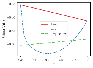
Figure 1: Motivating example. The “sa-rec” denotes the $(s,a)$-rectangular while the “d-rec” denotes the $d$-rectangular adopted by this paper. The “Proj. sa-rec” denotes the projected $(s,a)$-rectangular values into the linear space w.r.t. $\phi(s,a)$, which leads to the wrong direction. See Appendix A for details.

As shown by Wiesemann et al. (2013), computing an optimal robust policy for general ambiguity set is strongly NP-Hard. For computational tractability, Nilim & El Ghaoui (2005); Iyengar (2005) introduce the $(s,a)$-rectangular ambiguity set, where ${\mathcal{P}}_{h}=\prod_{(s,a)\in{\mathcal{S}}\times{\mathcal{A}}}{\mathcal{P}}_{h}(s,a)$ implies that the transition probability $P$ taking values independently for each state-action pair. The assumption ensures the perturbation of the transition probability for each $(s,a)$-pair is unrelated to others. However, the $(s,a)$-rectangular assumption may be prohibitively time-consuming when the state space or action space is large, as it requires to solve the robust optimization problem for each $(s,a)$-pair. More importantly, it may suffer over-conservatism, especially when the transition probabilities enjoy some inherent structure (Wiesemann et al., 2013; Goyal & Grand-Clement, 2022).

Prior to this work, the only attempts in linear function approximation for the robust RL are Tamar et al. (2013); Badrinath & Kalathil (2021), both sharing the same idea, i.e., first to obtain the robust value for each $(s,a)$-pair and then use a set of linear function basis to approximate the robust values for the whole ${\mathcal{S}}\times{\mathcal{A}}$. We use a motivating example with the inherent structure to compare our proposed algorithm with theirs to point out that directly projecting the robust values into the linear space might result in a poor approximation. We consider a continuous bandit case, which corresponds to the case of offline RL with $H=1$ and $S=1$. The action set is $[0,1]$. When taking the action $a=0$, we receive a reward $r_{0}$ drawing from $\mathcal{N}(1,1)$. If the action $a=1$ are chosen, the reward $r_{1}$ follows $\mathcal{N}(0,0.5^{2})$. For $a\in(0,1)$, its reward distribution $r_{a}$ is the mixture of $r_{0}$ and $r_{1}$, which means the reward follows $\mathcal{N}(1,1)$ w.p. $1-a$ and follows $\mathcal{N}(0,0.5^{2})$ w.p. $a$.

Since the problem enjoys a linear structure, using the linear function approximation to maintain the low-dimension representation is desirable. However, as shown in Figure 1, the projected robust values using Tamar et al. (2013); Badrinath & Kalathil (2021)’s methods are irrational due to the nonlinear nature of the $(s,a)$-uncertainty set. In particular, the projected algorithm behaves even more pessimistically than the $(s,a)$-rectangular for the actions close to $0$ or $1$. More importantly, it fails to preserve the order relationship between the robust values of actions $0$ and $1$, i.e., the robust value of action $0$ is higher than $1$ in the $(s,a)$-rectangular but becomes lower after projection, which will potentially lead to wrong decisions. Instead, our proposed algorithm based on the $d$-rectangular ambiguity set (see Section 4 for definition), recovers the robust values for action $0$ and $1$ while avoiding the over-conservatism of $a\in(0,1)$.

4 Linear Function Approximation

In this section, we assume the MDP enjoys the soft state-aggregation structure and introduce the so-called $d$-rectangular ambiguity set. We then propose our first algorithm, Distributional Robust Value Iteration with Linear function approximation (DRVI-L) with corresponding non-asymptotic suboptimality results.

Assumption 4.1 (State-Aggregation MDP).

The true transition model is soft state-aggregation w.r.t. $\phi$ and the reward function admit linear representation w.r.t. $\phi$ (Definition 2.1), i.e., $r_{h}\in\operatorname{Span}(\phi)$.

4.1 Ambiguity Set Structure

As shown in the motivating example, the $(s,a)$-rectangularity assumption can potentially yield over-conservative policy, especially when the problem enjoys some inherent structure. In this paper, we consider the problem with a linear structure, i.e., the transition model admits a soft stage aggregation (Definition 2.1), and the reward function also has a linear representation. Thus building the ambiguity set based on the specific MDP’s linear structure might be more natural and less conservative to derive an efficient solution.

To tackle the above challenges, we assume each factor lies in an ambiguity set, which is formally stated in the Assumption 4.2.

Assumption 4.2 ($d$-rectangular).

For each $h\in[H]$, we assume the ambiguity set ${\mathcal{P}}_{h}$ with radius $\rho$ admits the following structure for some probability distance $D:\mathbb{R}^{d}\times\mathbb{R}^{d}\rightarrow\mathbb{R}_{\geq 0}$,

$${\mathcal{P}}_{h}(\rho)=\left\{\left(\sum_{i=1}^{d}\phi_{i}(s,a)\psi^{\prime}_{h,i}(s^{\prime})\right)_{sas^{\prime}}:\forall D(\psi_{h,i}^{\prime},\psi_{h,i})\leq\rho\right\}.$$

Assumption 4.2 implies that the factors are unrelated and thus each factor $\psi_{h,i}$ can be chosen arbitrarily within the set ${\mathcal{P}}(\psi_{h,i};\rho)\coloneqq\{\psi_{h,i}^{\prime}:D(\psi_{h,i}^{\prime},\psi_{h,i})\leq\rho\}$ without affecting $\psi_{h,j}$ for $j\neq i$. Our offline DRRL problem with $d$-rectangular is formulated as

$$R(\pi;{\mathcal{P}})=\inf_{P\in{\mathcal{P}}(\rho)=\prod_{h=1}^{H}{\mathcal{P}}_{h}(\psi_{h,i};\rho)}R(\pi,P).$$ (4)

To provide a concrete algorithm design and corresponding suboptimality analysis, we choose $D$ as the KL divergence. The corresponding ambiguity for horizon $h$ and the $i$-th factor is denoted as ${\mathcal{P}}^{\operatorname{KL}}(\psi_{h,i};\rho)$ and the ambiguity set for horizon $h$ is denoted as ${\mathcal{P}}^{\operatorname{KL}}(\psi_{h};\rho)\coloneqq\prod_{i\in[d]}{\mathcal{P}}^{\operatorname{KL}}(\psi_{h,i};\rho)$. Hu & Hong (2013) proves a strong duality lemma to ensure the computational tractability of the distributionally robust optimization with KL divergence in Equation 4.

Lemma 4.1 (Hu & Hong (2013)).

Suppose $X\sim P$ has finite moment generating function in the neighborhood of zero. Then ,

$$\inf_{P^{\prime}:D_{\rm KL}(P^{\prime}\parallel P)\leq\rho}\mathbb{E}_{P^{\prime}}[X] =\sup_{\beta\geq 0}\{-\beta\log(Z)-\beta\cdot\rho\}$$

$$=\sup_{\beta\geq 0}\sigma(Z,\beta),$$ (5)

where $Z:=\mathbb{E}_{P}[e^{-X/\beta}]$.

When $\rho\to 0$, the LHS degrades to the non-robust view, i.e., $\mathbb{E}_{P}[X]$, and the optimum $\beta^{*}=\arg\sup_{\beta\geq 0}\sigma(Z,\beta)$ goes to infinity.

Based on Lemma 4.1, we can derive the following DR Bellman operator:

$$({\mathbb{B}}_{h}V)(s,a)=r(s,a)+\inf_{P_{h}\in{\mathcal{P}}^{\operatorname{KL}}(\psi_{h};\rho)}\mathbb{E}_{s^{\prime}\sim P_{h}(\cdot\lvert s,a)}[V(s^{\prime})]$$ (6)

$$=\phi(s,a)^{\top}(\theta_{h}+w_{h})=\phi(s,a)^{\top}\nu_{h},$$

where $w_{h,i}=\sup_{\beta\geq 0}\sigma(\mu_{h,i},\beta)$ and
$\mu_{h,i}\coloneqq\mathbb{E}_{\psi_{h,i}}[e^{-V(s^{\prime})/\beta}]$.

As shown above, the DR Bellman operator using the $d$-rectangular ambiguity set can maintain $\phi$ representation. We formalize it in Lemma 4.2 and based upon it, we design our DR variant of the value iteration algorithm.

Lemma 4.2.

For any policy $\pi$ and any epoch $h\in[H]$, the distributional robust Q-function is linear w.r.t. $\phi$. Moreover, $d({\mathbb{B}}_{h}{\mathcal{F}},{\mathcal{F}})=0$, where $d({\mathbb{B}}_{h}{\mathcal{F}},{\mathcal{F}})=\sup_{g\in{\mathcal{F}}}\inf_{f\in{\mathcal{F}}}\lVert f-{\mathbb{B}}_{h}g\rVert$ is the Bellman error (Munos & Szepesvári, 2008).

4.2 Distributionallly Robust Value Iteration

We are in the position to introduce the offline DRRL setting. The key challenge in the offline RL is that we restrict the computation of the policy with only access to some logged dataset instead of knowing the exact transition probability. Due to the lack of continuing interaction with the environment, the performance of the offline RL algorithm suffers from the insufficient coverage of the offline dataset. As a start, we first consider the uniformly “well-explored”, which is adopted widely in many offline RL works  (Jin et al., 2021; Duan et al., 2019; Xie et al., 2021).

Assumption 4.3 (Uniformly Well-explored Dataset).

Suppose $\mathcal{D}$ consists of $N$ trajectories $\{(s_{h}^{\tau},a_{h}^{\tau},r_{h}^{\tau})\}_{\tau,h=1}^{N,H}$ independently and identically induced by a fixed behavior policy $\overline{\pi}$ in the linear MDP. Meanwhile, suppose there exists an absolute constant $\underline{c}>0$ such that at each step $h\in[H]$,

$$\lambda_{\min}(\Sigma_{h})\geq\underline{c},\quad\text{ where }\Sigma_{h}=\mathbb{E}_{\overline{\pi}}[\phi(s_{h},a_{h})\phi(s_{h},a_{h})^{\top}].$$

Such an assumption requires the behavior policy to explore each feature dimension well, which might need to explore some state-action pairs that the optimal policy has seldom visited.

In principle, we construct the empirical version of the Bellman operator (see Equation 6) to approximate the true one, in particular, to approximate $\mu_{h,i}$. However, we cannot directly observe the samples from the distribution $\psi_{h,i}$ and thus fail to approximate it directly and estimate $\mu_{h,i}$. Instead, notice that

$$\mathbb{E}_{P_{s,a}}[e^{-V(s^{\prime})/\beta}]=\int_{s^{\prime}}e^{-V(s^{\prime})/\beta}P(s^{\prime}\lvert s,a)ds^{\prime}=\phi(s,a)^{\top}\mu_{h},$$

and samples from $P_{s,a}$ can be obtained, which motivates us to approximate $\mu_{h}$ by linear regression. We define the empirical mean squared errors as

$${\mathcal{E}}_{h,1}(\theta) =\sum_{\tau=1}^{K}(r_{h}^{\tau}-\phi(s_{h}^{\tau},a_{h}^{\tau})^{\top}\theta)^{2},$$ (7)

$${\mathcal{E}}_{h,2}(\mu) =\sum_{\tau=1}^{K}(e^{-V(s_{h+1}^{\tau})/\beta}-\phi(s_{h}^{\tau},a_{h}^{\tau})^{\top}\mu)^{2},$$ (8)

at each step $h\in[H]$. Correspondingly, we have

$$(\widehat{{\mathbb{B}}}_{h}V)(s,a) =\phi(s,a)^{\top}\widehat{\theta}_{h}+\phi(s,a)^{\top}\widehat{w}_{h},$$

$$\text{where}\quad\widehat{\theta}_{h} =\arg\min_{\theta\in{\mathbb{R}}^{d}}{\mathcal{E}}_{h,1}(\theta)+\lambda\cdot\lVert\theta\rVert^{2},$$

$$\widehat{\mu}_{h} =\arg\min_{\mu\in{\mathbb{R}}^{d}}{\mathcal{E}}_{h,2}(\mu)+\lambda\cdot\lVert\mu\rVert^{2},$$

$$\widehat{w}_{h,i} =\sup_{\beta\geq 0}\sigma(\widehat{\mu}_{h,i},\beta).$$

Here $\lambda>0$ is the regularization parameter.

Note that ridge penalization while ensuring numerical safe, inducing the solution $\widehat{\mu}_{h}$ to get close to zero. A close to zero $\widehat{\mu}_{h,i}$ would render $\sigma(\widehat{\mu}_{h,i},\beta)$ to approach infinity and destroy our estimation. Thus, we introduce a novel value shift technique in the $\widehat{w}_{h}$ by defining

$$\tilde{\sigma}(Z,\beta)=-\beta\log(Z+1)-\beta\cdot\rho,$$ (9)

to ensure $\log(Z+1)$ still remain valid even $Z$ approach zero. Correspondingly, we adopt the shifted variant of regression objective (see Equation 8), defined as

$$\tilde{{\mathcal{E}}}_{h,2}(\mu) =\sum_{\tau=1}^{K}((e^{-V(s_{h+1}^{\tau})/\beta}-1)-\phi(s_{h}^{\tau},a_{h}^{\tau})^{\top}\mu)^{2},$$

$$\widehat{\mu}_{h} =\arg\min_{\mu\in{\mathbb{R}}^{d}}\tilde{{\mathcal{E}}}_{h,2}(\mu)+\lambda\cdot\lVert\mu\rVert^{2},$$

$$\widehat{w}_{h,i} =\sup_{\beta\geq 0}\tilde{\sigma}(\widehat{\mu}_{h,i},\beta).$$ (10)

$\widehat{\theta}_{h}$ and $\widehat{w}_{h}$ have the closed form

$$\widehat{\theta}_{h}=\Lambda_{h}^{-1}\left(\sum_{\tau=1}^{K}\phi(s_{h}^{\tau},a_{h}^{\tau})r_{h}^{\tau}\right),$$

$$\widehat{\mu}_{h}=\Lambda_{h}^{-1}\left(\sum_{\tau=1}^{K}\phi(s_{h}^{\tau},a_{h}^{\tau})(e^{-V(s_{h+1}^{\tau}/\beta)}-1)\right),$$

$$\text{where}\quad\Lambda_{h}=\sum_{\tau=1}^{K}\phi(s_{h}^{\tau},a_{h}^{\tau})+\lambda\cdot I.$$

Our value shifting technique can ensure $\widehat{w}_{h}$ maintains a valid value no matter the quality of the estimator, which is the key to achieving the desired suboptimality that can nearly recover to that of the non-robust setting. We summarize our algorithm as Distributional Robust Value Iteration with Linear function approximation (DRVI-L) in Algorithm 1.

Before we present the suboptimality analysis for our algorithm 1, we impose the following Assumption 4.4 to assume a common known lower bound for the optimum of the KL optimization problem in Lemma 4.1. Such an assumption is also needed in the tabular case (Zhou et al., 2021b).

Assumption 4.4.

For each $h\in[H]$ and each $i\in[d]$, we denote

$$\beta_{h,i}^{*}= \operatorname{\arg\sup}_{\beta_{h,i}\geq 0}\sigma(\mu_{h,i},\beta_{h,i}).$$

We assume there is a common lower bound for $\{\beta_{h,i}^{*}\}_{h,i=1}^{H,d}$, i.e., we assume there exists a known $\underline{\beta}$ s.t. $0<\underline{\beta}\leq\min_{h\in[H],i\in[d]}\beta_{h,i}^{*}$.

By Proposition 2 in (Hu & Hong, 2013), $\beta_{h,i}^{*}=0$ when the worst case happens with sufficient large probability w.r.t. $\rho$, i.e., the larger the $\rho$, the easier we have $\beta_{h,i}^{*}=0$. In practice, we usually use a small $\rho$ to adapt to the problem without incurring over-conservatism, which utilize the advantage of DRO compared with other robustness notions (Ben-Tal & Nemirovski, 1998, 2000; Duchi & Namkoong, 2021).

Algorithm 1 DRVI-L

1:  Input: $\underline{\beta}$, $\mathcal{D}=\left\{\left(s_{h}^{\tau},a_{h}^{\tau},r_{h}^{\tau}\right)\right\}_{\tau,h=1}^{N,H}$.

2:  Init: $\widehat{V}_{H}=0$.

3:  for step $h=H$ to $1$ do

4:     $\Lambda_{h}\leftarrow\sum_{\tau=1}^{N}\phi\left(s_{h}^{\tau},a_{h}^{\tau}\right)\phi\left(s_{h}^{\tau},a_{h}^{\tau}\right)^{\top}+\lambda I$

5:     $\widehat{\theta}_{h}\leftarrow\Lambda_{h}^{-1}\left[\sum_{\tau=1}^{N}\phi(s_{h}^{\tau},a_{h}^{\tau})r_{h}^{\tau}\right]$

6:     if $h=H$ then

7:        $\widehat{w}_{H}\leftarrow 0$

8:     else

9:        Update $\widehat{w}_{h,i}$ with Equation 10.

10:     end if

11:     $\widehat{\nu}_{h}=\min(\widehat{\theta}_{h}+\widehat{w}_{h},H-h+1)_{+}$

12:     $\widehat{Q}_{h}(\cdot,\cdot)\leftarrow\phi(\cdot,\cdot)^{\top}\widehat{\nu}_{h}$

13:     $\widehat{\pi}_{h}(\cdot\mid\cdot)\leftarrow\arg\max_{\pi_{h}}\langle\widehat{Q}_{h}(\cdot,\cdot),\pi_{h}(\cdot\mid\cdot)\rangle_{\mathcal{A}}$

14:     $\widehat{V}_{h}(\cdot)\leftarrow\langle\widehat{Q}_{h}(\cdot,\cdot),\widehat{\pi}_{h}(\cdot\mid\cdot)\rangle_{\mathcal{A}}$

15:  end for

Theorem 4.1.

We set $\lambda=1$ in Algorithm 1. Under the Assumption 4.1, Assumption 4.3 and Assumption 4.4, when $N\geq 40/\underline{c}\cdot\log(4dH/\delta)$, we have the following holds with probability at least $1-\delta$,

$$\operatorname{SubOpt}(\widehat{\pi};{\mathcal{P}}) \leq c_{1}\underline{\beta}(e^{H/\underline{\beta}}-1)d^{1/2}\zeta_{1}^{1/2}H/N^{1/2}$$

$$+c_{2}\underline{\beta}^{1/2}(e^{H/\underline{\beta}}-1)\zeta_{2}^{1/2}H^{3/2}/N^{1/2}.$$

Here $\zeta_{1}=\log(2N+16Nd^{3/2}H^{2}e^{H/\underline{\beta}})$, $\zeta_{2}=\log(\frac{2dNH^{3}}{\delta\rho})$ and $c_{1}$ and $c_{2}$ are some absolute constants that only depend on $\underline{c}$.

Notice that the suboptimality of algorithm 1 mainly depends on the dimension $d$ instead of the size of the state-action space. Compared with tabular cases, e.g., (Zhou et al., 2021b; Yang et al., 2021a), which mainly bounds the finite sample error for each $(s,a)$ pair separately, Theorem 4.1 is derived by exploiting the linear structure shared by various $(s,a)$-pairs, building a novel $\epsilon$-net to control the finite sample error for whole linear function family space, and utilizing the power of our value shift algorithmic ingredient. The DRO ingredient requires to design a specific $\epsilon$-net for the function family that is different from the non-robust linear function approximation.

In particular, $\tilde{O}(d^{1/2}H^{3/2}\sqrt{\underline{\beta}}e^{H/\underline{\beta}}/N^{1/2})$ when $\underline{\beta}$ is relatively small, i.e., when the algorithm tends to learn a pessimistic view. When $\underline{\beta}\rightarrow\infty$, i.e., the algorithm is learning a nearly non-robust view, our bound reduces to $\tilde{O}(d^{1/2}H^{2}/N^{1/2})$, which recovers to the same dependence on $H$ compared with the non-robust PEVI algorithm in Jin et al. (2021) and achieve the optimal dependence on $N$ and $d$ in Yin et al. (2022). The gap in the $H$ is because we adopt a relatively simple algorithmic design framework to outline the first step in DRRL linear function approximation. Adopting the advance technique of Yin et al. (2022) may solve the gap and we leave it as a further direction.

5 Extensions

5.1 Beyond Uniformly Well-explored Dataset

In real applications, the data coverage may not be ideal as Assumption 4.3, which requires the behavior policy to explore all the feature dimensions with a sufficiently high exploration rate. Instead, we only require the behavior policy to have sufficient coverage of the features that the optimal policy will visit. Thus we design the pessimistic variant of our Algorithm 1, called the Pessimistic Distributionally Robust Value Iteration with Linear function approximation (PDRVI-L), by leveraging the idea of Jin et al. (2021). Under a weaker data coverage condition, sample efficiency can be obtained as long as the trajectory induced by the optimal policy $\pi^{*}$ is sufficiently covered by the dataset sufficiently well. We formalize this condition in Assumption 5.1.

Assumption 5.1 (Sufficient Coverage of the Optimal Policy).

Suppose there exists an absolute constant $c^{\dagger}>0$ such that

$$\Lambda_{h}\geq I+c^{\dagger}\cdot N\cdot d\cdot\mathbb{E}_{\pi^{*}}[(\phi_{i}(s_{h},a_{h})\mathds{1}_{i})(\phi_{i}(s_{h},a_{h})\mathds{1}_{i})^{\top}\lvert s_{1}=s],$$

$\forall s\in{\mathcal{S}},h\in[H],i\in[d]$, holds for probability at least $1-\delta$.

Compared with sufficient coverage condition in (Jin et al., 2021), our Assumption 5.1 requires the collected samples $\Lambda_{h}$ covers uniformly well for different dimension $i\in[d]$. Such a requirement comes from the ambiguity set constructed from the feature space. We summarize our algorithmic design in Algorithm 2, which is deferred to Appendix B. Compared with Algorithm 1, we subtract a pessimistic term $\gamma_{h}\sum_{i=1}^{d}\lVert\phi_{i}(s,a)\mathds{1}_{i}\rVert_{\Lambda_{h}^{-1}}$ from the estimated $Q$-value. This pessimistic term discourages our algorithm from choosing the action with less confidence. Compared with (Jin et al., 2021) which use $\gamma_{h}\lVert\phi(s,a)\rVert_{\Lambda_{h}^{-1}}$ as the pessimistic term in non-robust setting, ours is a larger penalization and adapt to the distributionally robust nature. Under the partial coverage condition for our dataset, our Algorithm 2 enjoys sample efficiency as concluded in the following theorem.

Theorem 5.1.

In Algorithm 2 we set $\lambda=1$ and

$$\gamma_{h} =c_{1}\underline{\beta}(e^{\frac{H-h}{\underline{\beta}}}\!-\!1)d\zeta_{3}^{1/2}+c_{2}\underline{\beta}^{1/2}(e^{\frac{H-h}{\underline{\beta}}}\!-\!1)H^{1/2}\zeta_{2}^{1/2},$$

where $\zeta_{2}$ is the same as in Theorem 4.1 and $\zeta_{3}=\log(2N+32N^{2}H^{3}d^{5/2}\zeta e^{2H/\beta})$ for some absolute constant $c_{1}$ and $c_{2}$ that are only dependent on $c^{\dagger}$. Then under the Assumption 4.1, 4.4 and 5.1, our algorithm 2 has the following guarantee with probability at least $1-\delta$,

$$\operatorname{SubOpt}(\widehat{\pi};{\mathcal{P}})\leq c_{1}\underline{\beta}(e^{H/\underline{\beta}}-1)d^{3/2}H\zeta_{3}^{1/2}/N^{1/2}$$

$$+ c_{2}\underline{\beta}^{1/2}(e^{H/\underline{\beta}}-1)d^{1/2}H^{3/2}\zeta_{2}^{1/2}/N^{1/2}.$$

This bound incurs an extra $d$ compared with Theorem 5.2 as a price to work for a weaker data coverage condition. In specific, the suboptimality for the Algorithm 2 is $\tilde{O}(d^{3/2}H^{3/2}\sqrt{\underline{\beta}}e^{H/\underline{\beta}}/N^{1/2})$ when $\underline{\beta}$ is relatively small. When $\underline{\beta}\rightarrow\infty$, i.e., the algorithm is learning a nearly non-robust view, the suboptimality reduces to $\tilde{O}(d^{3/2}H^{2}/N^{1/2})$, which recovers to the same dependence of $d$, $H$ and $N$ as Jin et al. (2021). Recently, Yin et al. (2022) improves the suboptimality bound to $\tilde{O}(d^{1/2}H^{3/2}/N^{1/2})$ with a complicate algorithm design. Instead, our paper is the first attempt to design linear function approximation to solve the distributionally robust offline RL problem. Thus we leave the improvement to the optimal rate as a further direction.

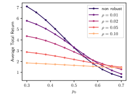
(a) Average Return

(b) $\|\widehat{V}_{1}-V^{*}_{1}\|$

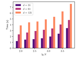
(c) Execution time

Figure 2: Results in American Option Experiment. (a) Average total return of different KL radius $\rho$ in the perturbed environments ($N=1000$, $d=61$). (b) Estimation error with different linear function dimension $d$’s and the sizes of dataset $N$’s ($\rho=0.01$). (c) Execution time for different $d$’s.

5.2 Model Misspecification

The state aggregation assumption may not be realistic when applied to the real-world dataset. In this subsection, we relax the assumption of the soft state-aggregation MDP to allow the true transition kernel is nearly a state-aggregation transition.

Assumption 5.2 (Model Misspecification in Transition Model).

We assume that for all $h\in[H]$, there exists $\tilde{P}_{h}\in\operatorname{Span}(\phi)$ and $\xi\geq 0$ such that each $(s,a)$, the true transition kernel $P_{h}(\cdot\lvert s,a)$ satisfies $\lVert P_{h}(\cdot\lvert s,a)-\tilde{P}_{h}(\cdot\lvert s,a)\rVert_{1}\leq\xi$. For the reward functions, without loss of generality we still assume that $r_{h}\in\operatorname{Span}(\phi)$ for all $h\in[H]$.

Theorem 5.2 (Model Misspecification).

We set $\lambda=1$ in Algorithm 1. Under the Assumption 4.3, 4.4 and 5.2, when $N\geq 40/\underline{c}\cdot\log(4dH/\delta)$, we have the following holds with probability at least $1-\delta$,

$$\operatorname{SubOpt}(\widehat{\pi};{\mathcal{P}})\leq c_{1}\underline{\beta}(e^{H/\underline{\beta}}-1)(\xi d^{1/2}+d^{1/2}\zeta_{1}^{1/2})H/N^{1/2}$$

$$\quad+c_{2}\underline{\beta}^{1/2}(e^{H/\underline{\beta}}-1)H^{3/2}\zeta_{2}^{1/2}/N^{1/2}+H(H-1)\xi/2.$$

Here $\zeta_{1}$ and $\zeta_{2}$ are the same in Theorem 4.1 and $c_{1}$ and $c_{2}$ are some absolute constants that only depend on $\underline{c}$.

Theorem 5.3 (Model Misspecification with Sufficient Coverage).

In Algorithm 2 we set $\lambda=1$ and

$$\gamma_{h} =c_{1}\underline{\beta}(e^{\frac{H-h}{\underline{\beta}}}\!-\!1)d\zeta_{3}^{1/2}+c_{2}\underline{\beta}^{1/2}(e^{\frac{H-h}{\underline{\beta}}}\!-\!1)H^{1/2}\zeta_{2}^{1/2},$$

where $\zeta_{2}$ and $\zeta_{3}$ are the same as in Theorem 5.1 and $c_{1},c_{2}\geq 1$ are some absolute constants that only involve $c^{\dagger}$. Then based on Assumptions 4.4, 5.1 and 5.2, our Algorithm 2 has the following guarantee with probability at least $1-\delta$,

$$\operatorname{SubOpt}(\widehat{\pi};{\mathcal{P}})\leq c_{1}\underline{\beta}(e^{H/\underline{\beta}}-1)(\xi d+d^{3/2}\zeta_{3}^{1/2})H/N^{1/2}$$

$$+c_{2}\underline{\beta}^{1/2}(e^{H/\underline{\beta}}-1)d^{1/2}H^{3/2}\zeta_{2}^{1/2}/N^{1/2}+H(H-1)\xi/2.$$

Theorem 5.2 implies that when the soft-state aggregation model is inexact up to $\xi$ total variation, there is an approximation gap in the policy’s performance $O(\xi\cdot(\underline{\beta}(e^{H/\underline{\beta}}-1)d^{1/2}+H^{2}))$ and $O(\xi\cdot(\underline{\beta}(e^{H/\underline{\beta}}-1)d+H^{2}))$ for our DRVI-L and PDRVI-L algorithms respectively. The level of degradation depends on the total-variation divergence between the true transition distribution and the robustness level we aim to achieve.

6 Experiment

We conduct the experiments to answer: (a) with linear function approximation, does distributionally robust value iteration perform better than the standard value iteration in the perturbed environments? (b) how does the linear dimension $d$ affect performance? We evaluate our algorithm in the American put option environment (Tamar et al., 2013; Zhou et al., 2021b). The experiment setup is classical and is deferred in the Appendix C.

We first compare distributionally robust and standard value iteration with the same linear function approximation. For both algorithms, we use $d=31$ and collect a dataset with 1000 trajectories in the environment with $p_{0}=0.5$. After training with different uncertainty ball radius $\rho$’s, we evaluate their average performance in the perturbed environment with different $p_{0}$’s. The results are depicted in Figure 2(a). As expected, the robust agent performs better than the non-robust one better in the perturbed environment with $p>0.55$. We also notice the policy with $\rho=0.01$ has a similar performance with the non-robust one in the nominal environment ($p_{0}=0.5$) and a much more robust performance across the perturbed environments, showing the superiority of our method.

Next, we investigate the effect of the linear function dimension. We fix the number of trajectories and compare $\|\widehat{V}_{1}-V^{*}_{1}\|$ with different $d$’s. We repeat each experiment 20 times and show the average results in Figure 2(b). As our theoretical analysis points out, the smaller $d$ leads to a lower estimation error and higher approximation error with the same data size. The misspecification of the linear transition model will bring an intrinsic bias to the value estimation. Yet, the proper bias brings lower error with limited data, which is essential for offline learning.

We show the computational efficiency of the proposed method, which is measured by the average execution time (see Figure 2(c)). The result shows that the average execution time linearly depends on the $d$, which indicates that the computing bottleneck of the algorithm is solving the dual problems (line 9 in Algorithm 1). All the experiments are finished on a server with an AMD EPYC 7702 64-Core Processor CPU.

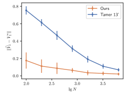
Figure 3: Compare the estimation error with RPVI.

Finally, we compare our method with the robust projected VI (RPVI) (Tamar et al., 2013), in which the robust values are first calculated for each $(s,a)$-pair and then projected into the linear function space. Under the same function class with $d=61$, we compare their value difference with the optimal value in Figure 3, where our algorithm has more accurate estimations with the varying $N$. In addition, since RPVI solves the robust problem for each $(s,a)$, its execution time linearly depends on the sample size $N$. For instance, with $d=61$ and $N=1000$, RPVI needs over $1000s$, while our DRVI-L can finish less than $10s$. The details of reproduction are shown in Appendix I

Appendix A Details of the motivating example

For convenience, given a r.v. $X$, we denote its distributional robust value (refer Lemma 4.1) as $g(X,\rho)=\sup_{\beta\geq 0}\{-\beta\log(\mathbb{E}_{X\sim P}[e^{X/\beta}])-\beta\cdot\rho\}.$ For any action $a$, the corresponding reward distribution is

$$r_{a}\sim\begin{cases}\mathcal{N}(1,1)&{\rm w.p.}\quad 1-a\\ \mathcal{N}(0,0.5)&{\rm w.p.}\quad a\end{cases}$$ (11)

Based on the definition of $(s,a)$-rectangular, the robust action-value function $Q_{\rm sa}(a)=g(r_{a},1)$. The projected value function is approximated with a linear function $Q_{\rm proj}(a)=[1-a;a]^{\top}w$, where $w=\operatorname*{arg\,min}_{u}\mathbb{E}_{a\sim U[0,1]}(V_{\rm sa}(a)-[1-a;a]^{T}u)^{2}$. The $d$-rectangular robust action-value function is $Q_{\rm d}(a)=(1-a)g(r_{0},1)+ag(r_{1},1)$.

Appendix B Algorithm Design for the PDRVI-L

Algorithm 2 PDRVI-L

1:  Input: $\underline{\beta}$, $\mathcal{D}=\left\{\left(s_{h}^{\tau},a_{h}^{\tau},r_{h}^{\tau}\right)\right\}_{\tau,h=1}^{N,H}$.

2:  Init: $\widehat{V}_{H}=0$.

3:  for step $h=H$ to $1$ do

4:     $\Lambda_{h}\leftarrow\sum_{\tau=1}^{N}\phi\left(s_{h}^{\tau},a_{h}^{\tau}\right)\phi\left(s_{h}^{\tau},a_{h}^{\tau}\right)^{\top}+\lambda I$

5:     $\widehat{\theta}_{h}\leftarrow\Lambda_{h}^{-1}\left[\sum_{\tau=1}^{N}\phi(s_{h}^{\tau},a_{h}^{\tau})r_{h}^{\tau}\right]$

6:     if $h=H$ then

7:        $\widehat{w}_{H}\leftarrow 0$

8:     else

9:        Update $\widehat{w}_{h,i}$ with Equation 10.

10:     end if

11:     $\widehat{\nu}_{h}=\min(\widehat{\theta}_{h}+\widehat{w}_{h},H-h+1)_{+}$

12:     $\widehat{Q}_{h}(\cdot,\cdot)\leftarrow\phi(\cdot,\cdot)^{\top}\widehat{\nu}_{h}-\gamma_{h}\sum_{i=1}^{d}\lVert\phi_{i}(s,a)\mathds{1}_{i}\rVert_{\Lambda_{h}^{-1}}$

13:     $\widehat{\pi}_{h}(\cdot\mid\cdot)\leftarrow\arg\max_{\pi_{h}}\langle\widehat{Q}_{h}(\cdot,\cdot),\pi_{h}(\cdot\mid\cdot)\rangle_{\mathcal{A}}$

14:     $\widehat{V}_{h}(\cdot)\leftarrow\langle\widehat{Q}_{h}(\cdot,\cdot),\widehat{\pi}_{h}(\cdot\mid\cdot)\rangle_{\mathcal{A}}$

15:  end for

Appendix C Experiment Setup

We assume that the price follows Bernoulli distribution (Cox et al., 1979),

$$s_{h+1}=\begin{cases}c_{u}s_{h},&\text{ w.p. }p_{0}\\ c_{d}s_{h},&\text{ w.p. }1-p_{0}\end{cases}$$ (12)

where the $c_{u}$ and $c_{d}$ are the price up and down factors and $p_{0}$ is the probability that the price goes up. The initial price $s_{0}$ is uniformly sampled from $[\kappa-\epsilon,\kappa+\epsilon]$, where $\kappa=100$ is the strike price and $\epsilon=5$ in our simulation. The agent can take an action to exercise the option ($a_{h}=0$) or not exercise ($a_{h}=1$) at the time step $h$. If exercising the option, the agent receives a reward $\max(0,\kappa-s_{h})$ and the state transits into an exit state. Otherwise, the price will fluctuate based on the above model and no reward will be assigned. In our experiments, we set $H=20$, $c_{u}=1.02$, $c_{d}=0.98$. We limit the price in $[80,140]$ and discretize with the precision of 1 decimal place. Thus the state space size $|\mathcal{S}|=602$.

Since $Q(s_{h},a=1)=\max(0,\kappa-s_{h})$ is known in advance, we do not need to do any approximation for $a_{h}=1$, and only need to estimate $\widehat{Q}(s_{h},a=0)=\phi(s_{h})^{\top}\widehat{w}_{h}$. The features are chosen as $\phi(s_{h})=[\varphi(s_{h},s_{1}),\dots,\varphi(s_{h},s_{d})]^{\top}$, where $s_{1},\dots,s_{d}$ are selected anchor states and $\varphi(s_{h},s_{i}),\forall i\in[d]$ is the pairwise similarity measure. In particular, we set $s_{1}=s_{\rm min}=80,s_{d}=s_{\rm max=}140$, and $\Delta=s_{i+1}-s_{i}=(s_{\rm max}-s_{\rm min})/(d-1),\forall i\in[d-1]$. The similarity measure $\varphi(s_{h},s_{i})=\operatorname{max}(0,1-|s_{h}-s_{i}|/\Delta),\forall i\in[d]$, which is the partition to the nearest anchor states. Before training the agent, we collect data with a fixed behavior policy for $N$ trajectories. Since taking $a_{h}=1$ will terminate the episode, it is helpless for learning the transition model. Hence, we use a fixed policy to collect data, which always chooses $a_{h}=0$.

Appendix D Proof of Section 4

Lemma D.1.

Let $\pi=\{\pi_{h}\}_{h=1}^{H}$ and $\pi^{\prime}=\{\pi_{h}^{\prime}\}_{h=1}^{H}$ be any two policies and let $\{\widehat{Q}_{h}\}_{h=1}^{H}$ be any estimated Q-functions. For all $h\in[H]$, we define the estimated value function $\widehat{V}_{h}:\mathcal{S}\rightarrow\mathcal{R}$ by setting $\widehat{V}_{h}(s)=\langle\widehat{Q}_{h}(s,\cdot),\pi_{h}(\cdot\lvert s)\rangle_{\mathcal{A}}$ for all $s\in\mathcal{S}$. For all $s\in\mathcal{S}$, we have

$$\widehat{V}_{1}(s)-V_{1}^{\pi^{\prime}}(s) =\sum_{h=1}^{H}\mathbb{E}_{\pi^{\prime}}[\iota_{h}(s_{h},a_{h})\lvert s_{1}=s]+\sum_{h=1}^{H}\mathbb{E}_{\pi^{\prime}}[\langle\widehat{Q}_{1}(s,\cdot),\pi_{h}(\cdot\lvert s_{h})-\pi^{\prime}_{h}(\cdot\lvert s_{h})\rangle\lvert s_{1}=s],$$

where

$$\iota_{h}(s,a)=\widehat{Q}_{h}(s,a)-(r_{h}(s,a)+\inf_{P_{h+1}\in{\mathbb{P}}_{h+1}(\cdot|s,a)}\mathbb{E}_{s^{\prime}\sim P_{h+1}}[\widehat{V}_{h+1}(s^{\prime})]).$$

Proof.

$$\widehat{V}_{h}(s)-V_{h}^{\pi^{\prime}}(s) =\langle\widehat{Q}_{h}(s,\cdot),\pi_{h}(\cdot\lvert s)\rangle-\langle Q_{h}^{\pi^{\prime}}(s,\cdot),\pi_{h}^{\prime}(\cdot\lvert s)\rangle$$

$$=\langle\widehat{Q}_{h}(s,\cdot)-Q_{h}^{\pi^{\prime}}(s,\cdot),\pi_{h}^{\prime}(\cdot\lvert s)\rangle+\langle\widehat{Q}_{h}(s,\cdot),\pi_{h}(\cdot\lvert s)-\pi_{h}^{\prime}(\cdot\lvert s)\rangle$$

$$=\mathbb{J}_{h}(\widehat{Q}_{1}(s,\cdot)-Q_{h}^{\pi^{\prime}}(s,\cdot))+\xi_{h},$$

where $\mathbb{J}_{h}(f)=\langle f(s,\cdot),\pi_{h}^{\prime}(\cdot\lvert s)\rangle$. Moreover, we denote

$$\iota_{h}(s,a)=\widehat{Q}_{h}(s,a)-(r_{h}(s,a)+\inf_{P_{h+1}\in{\mathbb{P}}_{h+1}(\cdot|s,a)}\mathbb{E}_{s^{\prime}\sim P_{h+1}}[\widehat{V}_{h+1}(s^{\prime})]),$$

thus

$$\widehat{Q}_{h}(s,a)=r_{h}(s,a)+\inf_{P_{h+1}\in{\mathbb{P}}_{h+1}(\cdot\lvert s,a)}\mathbb{E}_{s^{\prime}\sim P_{h+1}}[\widehat{V}_{h+1}(s^{\prime})]+\iota_{h}$$

and

$$Q_{h}^{\pi^{\prime}}(s,a)=r_{h}(s,a)+\inf_{P_{h+1}\in{\mathbb{P}}_{h+1}(\cdot\lvert s,a)}\mathbb{E}_{s^{\prime}\sim P_{h+1}}[V_{h+1}^{\pi^{\prime}}(s^{\prime})],$$

which implies

$$\widehat{Q}_{h}(s,a)-Q_{h}^{\pi^{\prime}}(s,a) =\inf_{P_{h+1}\in{\mathbb{P}}_{h+1}(\cdot\lvert s,a)}\mathbb{E}_{s^{\prime}\sim P_{h+1}}(\widehat{V}_{h+1}(s^{\prime})-V_{h+1}^{\pi^{\prime}}(s^{\prime}))+\iota_{h}$$

$$\coloneqq\tilde{{\mathbb{P}}}_{h}(\widehat{V}_{h+1}-V_{h+1}^{\pi^{\prime}})+\iota_{h},$$

where $\tilde{{\mathbb{P}}}_{h}[H(s^{\prime})]\coloneqq\inf_{P_{h+1}\in{\mathbb{P}}_{h+1}(\cdot\lvert s,a)}\mathbb{E}_{s^{\prime}\sim P_{h+1}}[H(s^{\prime})]$. Thus we have

$$\widehat{V}_{h}(s)-V_{h}^{\pi^{\prime}}(s) =(\mathbb{J}_{h}\tilde{\mathbb{P}}_{h})(\widehat{V}_{h+1}-V_{h+1}^{\pi^{\prime}})+\mathbb{J}_{h}\iota_{h}+\xi_{h}$$

$$\widehat{V}_{1}(s)-V_{1}^{\pi^{\prime}}(s) =(\prod_{h=1}^{H}\mathbb{J}_{h}\tilde{\mathbb{P}}_{h})(\widehat{V}_{H+1}-V_{H+1}^{\pi^{\prime}})+\sum_{h=1}^{H}(\prod_{i=1}^{h-1}\mathbb{J}_{i}\tilde{{\mathbb{P}}}_{j})\iota_{j}+(\sum_{h=1}^{H}\prod_{i=1}^{h-1})\xi_{i}$$

$$=\sum_{h=1}^{H}(\prod_{i=1}^{h-1}\mathbb{J}_{i}\tilde{{\mathbb{P}}}_{j})\iota_{j}+(\sum_{h=1}^{H}\prod_{i=1}^{h-1})\xi_{i}$$

$$=\sum_{h=1}^{H}\mathbb{E}_{\pi^{\prime}}[\iota_{h}(s_{h},a_{h})\lvert s_{1}=s]+\sum_{h=1}^{H}\mathbb{E}_{\pi^{\prime}}[\langle\widehat{Q}_{1}(s,\cdot),\pi_{h}(\cdot\lvert s_{h})-\pi^{\prime}_{h}(\cdot\lvert s_{h})\rangle\lvert s_{1}=s],$$

where the second equality is because $\widehat{V}_{H+1}=V_{H+1}^{\pi^{\prime}}=\mathbf{0}$ and $\iota_{h}=\iota_{h}(s_{h},a_{h})$. ∎

Lemma D.2 (Decomposition of Suboptimality (DRO version)).

$$\begin{aligned} &\operatorname{SubOpt}(\widehat{\pi};{\mathcal{P}})=\sum_{h=1}^{H}\mathbb{E}_{\widehat{\pi}}\left[\iota_{h}\left(s_{h},a_{h}\right)\mid s_{1}\sim\mu\right]-\sum_{h=1}^{H}\mathbb{E}_{\pi^{*}}\left[\iota_{h}\left(s_{h},a_{h}\right)\mid s_{1}\sim\mu\right]\\ &+\sum_{h=1}^{H}\mathbb{E}_{\pi^{*}}\left[\left\langle\widehat{Q}_{h}\left(s_{h},\cdot\right),\pi_{h}^{*}\left(\cdot\mid s_{h}\right)-\widehat{\pi}_{h}\left(\cdot\mid s_{h}\right)\right\rangle_{\mathcal{A}}\mid s_{1}\sim\mu\right],\end{aligned}$$

where

$$\iota_{h}(s,a)\coloneqq\widehat{Q}_{h}(s,a)-(r_{h}(s,a)+\inf_{P_{h+1}\in{\mathbb{P}}_{h+1}(\cdot\lvert s,a)}\mathbb{E}_{s^{\prime}\sim P_{h+1}}[\widehat{V}_{h+1}(s^{\prime})]).$$

Proof.

By the definition above, the suboptimality of the policy $\hat{\pi}$ can be decomposed as

$$\operatorname{SubOpt}(\widehat{\pi};{\mathcal{P}}) =\underbrace{(\mathbb{E}_{s\sim\mu}[V^{*}_{1}(s)]-\mathbb{E}_{s\sim\mu}[\widehat{V}_{1}(s)])}_{\text{I}}+\underbrace{(\mathbb{E}_{s\sim\mu}[\widehat{V}_{1}(s)]-\mathbb{E}_{s\sim\mu}[V_{1}^{\widehat{\pi}}(s)])}_{\text{II}},$$ (13)

where $\{\widehat{V}_{h}\}_{h=1}^{H}$ are the estimated value functions constructed by any algorithm.

Apply Lemma D.1 to the I term in equation 13 with $\pi=\widehat{\pi}$, $\pi^{\prime}=\pi^{*}$ and $\{\widehat{Q}_{h}\}_{h=1}^{H}$ being the estimated Q-functions constructed by our algorithm 1, we have

$$\widehat{V}_{1}(s)-V_{1}^{*}(s)=\sum_{h=1}^{H}\mathbb{E}_{\pi^{*}}[\langle\widehat{Q}_{h}(s_{h},\cdot),\widehat{\pi}_{h}(\cdot\lvert s_{h})-\pi^{*}_{h}(\cdot\lvert s_{h})\rangle\lvert s_{1}=s]+\sum_{h=1}^{H}\mathbb{E}_{\pi^{*}}[\iota_{h}(s_{h},a_{h})\lvert s_{1}=s].$$ (14)

Similarily, apply Lemma D.1 to the II term in equation 13 with $\pi=\pi^{\prime}=\widehat{\pi}$ and $\{\widehat{Q}_{h}\}_{h=1}^{H}$ being the estimated Q-functions constructed by our algorithm 1, we have

$$\widehat{V}_{1}(s)-V_{1}^{\widehat{\pi}}(s)=\sum_{h=1}^{H}\mathbb{E}_{\widehat{\pi}}[\iota_{h}(s_{h},a_{h})\lvert s_{1}=s].$$ (15)

Putting equation 14 and equation 15 into equation 13 we yield the desired conclusions. ∎

Proof of Lemma 4.2 .

Recall the Bellman equation for the $d$-rectangular robust MDP (Equation 6):

$$({\mathbb{B}}_{h}V)(s,a) =r(s,a)+\inf_{P_{h}\in{\mathcal{P}}^{\operatorname{KL}}(\psi_{h};\rho)}\mathbb{E}_{s^{\prime}\sim P_{h}(\cdot\lvert s,a)}[V(s^{\prime})]$$ (16)

$$=\sum_{i\in[d]}\phi_{i}(s,a)\theta_{h,i}+\sum_{i\in[d]}\phi_{i}(s,a)\min_{\psi^{\prime}_{h,i}\in{\mathcal{P}}^{\operatorname{KL}}(\psi_{h,i};\rho)}\psi_{h,i}^{\prime\top}V$$

Since $M\in{\mathcal{M}}^{\operatorname{rob}}$, from the proof of above that for any $f\in{\mathcal{F}}$, we have ${\mathbb{B}}_{h}f\in{\mathcal{F}}$ for any $h\in[H]$, which finish the second part of the proof of lemma 4.2. ∎

Lemma D.3.

For any fix $h\in[H]$ and $i\in[d]$, we denote

$$\beta^{*}_{h,i}\in\operatorname*{arg\,max}_{\beta_{h,i}\geq 0}\{-\beta_{h,i}\cdot\mathbb{E}_{\psi_{h,i}}[e^{-V_{h+1}(s^{\prime})/\beta_{h,i}}]-\beta_{h,i}\rho\}.$$

Then $\beta^{*}_{h,i}\leq\overline{\beta}\coloneqq\frac{H-h+1}{\rho}$.

Proof.

This proof is by invoking the part 2 in the Lemma 4 in (Zhou et al., 2021b) with $M=H$. ∎

Thus in the following, we consider the variant of the dual form of the KL optimization,

$$\sup_{\beta_{h,i}\in[0,\overline{\beta}]}\{-\beta_{h,i}\cdot\mathbb{E}_{\psi_{h,i}}[e^{-V_{h+1}(s^{\prime})/\beta_{h,i}}]-\beta_{h,i}\rho\}.$$

Appendix E Proof of Theorem 5.2

Before we start the proof, it is obvious to note that $\sum_{i=1}^{d}\phi_{i}(s,a)=1,\forall(s,a)\in{\mathcal{S}}\times{\mathcal{A}}$ under the Assumption 4.1. In this section, we mainly prove the Theorem 5.2. By setting the model mis-specification $\xi=0$, we can recover the results in Theorem 4.1.

Proposition E.1.

With probability at least $1-\delta$, for all $h\in[H]$, we have

$$\iota_{h}(s,a)\leq \underline{\beta}(e^{H/\underline{\beta}}-1)(2\xi\sqrt{d}+10\sqrt{d\zeta_{1}})\sum_{i=1}^{d}\lVert\phi_{i}(s,a)\mathds{1}_{i}\rVert_{\Lambda_{h}^{-1}}+2\sqrt{2}\sqrt{\underline{\beta}}(e^{H/\underline{\beta}}-1)\sqrt{H\zeta_{2}}\sum_{i=1}^{d}\lVert\phi_{i}(s,a)\mathds{1}_{i}\rVert_{\Lambda_{h}^{-1}}+(H-h)\xi,$$

for $\zeta_{1}=\log(2N+16Nd^{3/2}H^{2}e^{H/\underline{\beta}})$ and $\zeta_{2}=\log(\frac{2dNH^{3}}{\delta\rho})$.

Proof.

From the DRO Bellman optimality equation and Lemma 4.1, we denote

$$({\mathbb{B}}_{h}\widehat{V}_{h+1})(s,a) =r_{h}(s,a)+\inf_{P_{h+1}\in{\mathbb{P}}_{h+1}}\ E_{P_{h+1}(\cdot\lvert s,a)}[\widehat{V}_{h+1}(s^{\prime})]$$

$$=r_{h}(s,a)+\inf_{\tilde{P}_{h+1}\in\tilde{{\mathbb{P}}}_{h+1}}\ E_{\tilde{P}_{h+1}(\cdot\lvert s,a)}[\widehat{V}_{h+1}(s^{\prime})]$$

$$\quad+(\inf_{P_{h+1}\in{\mathbb{P}}_{h+1}}\ E_{P_{h+1}(\cdot\lvert s,a)}[\widehat{V}_{h+1}(s^{\prime})]-\inf_{\tilde{P}_{h+1}\in\tilde{{\mathbb{P}}}_{h+1}}\ E_{\tilde{P}_{h+1}(\cdot\lvert s,a)}[\widehat{V}_{h+1}(s^{\prime})])$$

$$=\sum_{i=1}^{d}\phi_{i}(s,a)\theta_{h,i}+\sum_{i=1}^{d}\phi_{i}(s,a)\max_{\beta_{h,i}\in[\underline{\beta},\overline{\beta}]}\{-\beta_{h,i}\cdot\log(\mathbb{E}_{\psi_{h,i}}[e^{-\widehat{V}_{h+1}(s^{\prime})/\beta_{h,i}}])-\beta_{h,i}\rho\}$$

$$\quad+(H-h)\xi.$$

Combined with the empirical Bellman operator in our algorithm 1,

$$\iota_{h}(s,a) =({\mathbb{B}}_{h}\widehat{V}_{h+1})(s,a)-(\widehat{{\mathbb{B}}}_{h}\widehat{V}_{h+1})(s,a)$$ (17)

$$=\phi(s,a)^{\top}(\theta_{h}-\widehat{\theta}_{h})+\phi(s,a)^{\top}(w_{h}-\widetilde{w}_{h})+(H-h)\xi,$$

where $w_{h,i}\coloneqq\max_{\beta_{h,i}\in[\underline{\beta},\overline{\beta}]}\{-\beta_{h,i}\log(\mathbb{E}_{\psi_{h,i}}[e^{-\widehat{V}_{h+1}(s^{\prime})/\beta_{h,i}}])-\beta_{h,i}\rho\}$ and
$\widetilde{w}_{h,i}\coloneqq\max_{\beta_{h,i}\in[\underline{\beta},\overline{\beta}]}\{-\beta_{h,i}\log(\widehat{\psi}_{h,i}^{\top}[e^{-\widehat{V}_{h+1}(s^{\prime})/\beta_{h,i}}-1]+1)-\beta_{h,i}\rho\}$.

Step 1: we analyze the error in the reward estimation, i.e., $\phi(s,a)^{\top}(\theta_{h}-\widehat{\theta}_{h})$.

$$\phi(s,a)^{\top}(\theta_{h}-\widehat{\theta}_{h}) =\phi(s,a)^{\top}\Lambda_{h}^{-1}\Lambda_{h}\theta_{h}-\phi(s,a)^{\top}\Lambda_{h}^{-1}[\sum_{\tau=1}^{N}\phi(s_{h}^{\tau},a_{h}^{\tau})r_{h}(s_{h}^{\tau},a_{h}^{\tau})]$$ (18)

$$=\phi(s,a)^{\top}\Lambda_{h}^{-1}\Lambda_{h}\theta_{h}-\phi(s,a)^{\top}\Lambda_{h}^{-1}[\sum_{\tau=1}^{N}\phi(s_{h}^{\tau},a_{h}^{\tau})\phi(s_{h}^{\tau},a_{h}^{\tau})^{\top}\theta_{h}]$$

$$=\phi(s,a)^{\top}\Lambda_{h}^{-1}\Lambda_{h}\theta_{h}-\phi(s,a)^{\top}\Lambda_{h}^{-1}(\Lambda_{h}-\lambda I)\theta_{h}$$

$$=\lambda\phi(s,a)^{\top}\Lambda_{h}^{-1}\theta_{h}$$

$$\leq\lambda\lVert\theta_{h}\rVert_{\Lambda_{h}^{-1}}\lVert\phi(s,a)\rVert_{\Lambda^{-1}_{h}}$$

$$\leq\sqrt{d\lambda}\lVert\phi(s,a)\rVert_{\Lambda_{h}^{-1}}$$

$$\leq\sqrt{d\lambda}\sum_{i=1}^{d}\lVert\phi_{i}(s,a)\mathds{1}_{i}\rVert_{\Lambda_{h}^{-1}}.$$

Here the last inequality is from

$$\lVert\theta_{h}\rVert_{\Lambda_{h}^{-1}}=\sqrt{\theta_{h}^{\top}\Lambda_{h}^{-1}\theta_{h}}\leq\lVert\Lambda_{h}^{-1}\rVert^{1/2}\lVert\theta_{h}\rVert\leq\sqrt{d/\lambda},$$

by using the fact that $\lVert\Lambda_{h}^{-1}\rVert\leq\lambda^{-1}$ and the Definition 2.1.

Step 2: we turn to the estimation error from the transition model, i.e., $\phi(s,a)^{\top}(w_{h}-\widehat{w}_{h})$. We define two auxiliary functions:

$$\hat{g}_{h,i}(\beta)\coloneqq-\beta\cdot\log(\widehat{\psi}_{h,i}^{\top}[e^{-\widehat{V}_{h+1}(s^{\prime})/\beta}-1]+1)-\beta\rho,$$

and

$$g_{h,i}(\beta)\coloneqq-\beta\cdot\log(\mathbb{E}_{\psi_{h,i}}[e^{-\widehat{V}_{h+1}(s^{\prime})/\beta}])-\beta\rho.$$

Then

$$\lvert\sum_{i\in[d]}\phi_{i}(s,a)(w_{h,i}-\widetilde{w}_{h,i})\rvert$$

$$\leq\sum_{i\in[d]}\lvert\phi_{i}(s,a)(w_{h,i}-\widetilde{w}_{h,i})\rvert$$ (19)

$$=\sum_{i\in[d]}\phi_{i}(s,a)\lvert\max_{\beta_{h,i}\in[\underline{\beta},\overline{\beta}]}g_{h,i}(\beta_{h,i})-\max_{\beta_{h,i}\in[\underline{\beta},\overline{\beta}]}\hat{g}_{h,i}(\beta_{h,i})\rvert$$

$$\leq\sum_{i\in[d]}\phi_{i}(s,a)\max_{\beta_{h,i}\in[\underline{\beta},\overline{\beta}]}\lvert g_{h,i}(\beta_{h,i})-\hat{g}_{h,i}(\beta_{h,i})\rvert$$

$$=\sum_{i\in[d]}\phi_{i}(s,a)\max_{\beta_{h,i}\in[\underline{\beta},\overline{\beta}]}\{\lvert\beta_{h,i}\cdot(\log(\widehat{\psi}_{h,i}^{\top}[(e^{-\widehat{V}_{h+1}(s^{\prime})/\beta_{h,i}}-1)]+1)-\log(\mathbb{E}_{\psi_{h,i}}[e^{-\widehat{V}_{h+1}(s^{\prime})/\beta_{h,i}}]))\rvert\}$$

$$=\sum_{i\in[d]}\phi_{i}(s,a)\max_{\beta_{h,i}\in[\underline{\beta},\overline{\beta}]}\{\lvert\beta_{h,i}\cdot(\log(\widehat{\psi}_{h,i}^{\top}[e^{(H-\widehat{V}_{h+1}(s^{\prime}))/\beta_{h,i}}-e^{H/\beta_{h,i}}]+e^{H/\beta_{h,i}})-\log(\mathbb{E}_{\psi_{h,i}}[e^{(H-\widehat{V}_{h+1}(s^{\prime}))/\beta_{h,i}}]))\rvert\}$$

$$\leq\sum_{i\in[d]}\phi_{i}(s,a)\max_{\beta_{h,i}\in[\underline{\beta},\overline{\beta}]}\{\lvert\beta_{h,i}\cdot(\widehat{\psi}_{h,i}^{\top}[e^{(H-\widehat{V}_{h+1}(s^{\prime}))/\beta_{h,i}}-e^{H/\beta_{h,i}}]+e^{H/\beta_{h,i}}-\mathbb{E}_{\psi_{h,i}}[e^{(H-\widehat{V}_{h+1}(s^{\prime}))/\beta_{h,i}}])\rvert\},$$ (20)

where the last inequality follows from the fact H.2 by setting $x=\beta_{h,i}\log(\widehat{\psi}_{h,i}^{\top}[e^{(H-\widehat{V}_{h+1}(s))/\beta_{h,i}}-e^{H/\beta_{h,i}}]+e^{H/\beta_{h,i}})$ and $y=\beta_{h,i}\log\mathbb{E}_{\psi_{h,i}}[e^{(H-\widehat{V}_{h+1}(s))/\beta_{h,i}}]$. To ease the presentation, we index the finite states from $1$ to $S$ and introduce the vector $\widehat{V}_{h+1}\in\mathbb{R}^{S}$ where $[\widehat{V}_{h+1}]_{j}=\widehat{V}_{h,i}(s_{j})$ and $[H-\widehat{V}_{h+1}]_{j}=H-\widehat{V}_{h+1}(s_{j})$.

We denote $\mathds{1}_{j}\in\mathbb{R}^{d\times 1}$ with the $j$-the component as 1 and the other components are 0 and $\bm{1}\in\mathbb{R}^{S}$ is a all-one vector. Notice that

$$\mathbb{E}_{\psi_{h,i}}[e^{(H-\widehat{V}_{h+1}(s^{\prime}))/\beta_{h,i}}]$$

$$=\mathbb{E}_{\psi_{h,i}}[e^{(H-\widehat{V}_{h+1}(s^{\prime}))/\beta_{h,i}}-e^{H/\beta_{h,i}}]+e^{H/\beta_{h,i}}$$

$$=\psi_{h,i}^{\top}(e^{(H-\widehat{V}_{h+1})/\beta_{h,i}}-e^{H/\beta_{h,i}})+e^{H/\beta_{h,i}}$$

$$=\mathds{1}_{i}^{\top}\psi_{h}^{\top}(e^{(H-\widehat{V}_{h+1})/\beta_{h,i}}-e^{H/\beta_{h,i}})+e^{H/\beta_{h,i}}$$

$$=\mathds{1}_{i}^{\top}\Lambda_{h}^{-1}\Lambda_{h}\psi_{h}^{\top}(e^{(H-\widehat{V}_{h+1})/\beta_{h,i}}-e^{H/\beta_{h,i}})+e^{H/\beta_{h,i}}$$

$$=\mathds{1}_{i}^{\top}\Lambda_{h}^{-1}(\sum_{\tau=1}^{N}\phi(s_{h}^{\tau},a_{h}^{\tau})\phi(s_{h}^{\tau},a_{h}^{\tau})^{\top}+\lambda I)\psi_{h}^{\top}(e^{(H-\widehat{V}_{h+1})/\beta_{h,i}}-e^{H/\beta_{h,i}})+e^{H/\beta_{h,i}}$$

$$=\mathds{1}_{i}^{\top}\Lambda_{h}^{-1}\sum_{\tau=1}^{N}\phi(s_{h}^{\tau},a_{h}^{\tau})\phi(s_{h}^{\tau},a_{h}^{\tau})^{\top}\psi_{h}^{\top}(e^{(H-\widehat{V}_{h+1})/\beta_{h,i}}-e^{H/\beta_{h,i}})$$

$$\quad+\lambda\mathds{1}_{i}^{\top}\Lambda_{h}^{-1}\psi^{\top}_{h}(e^{(H-\widehat{V}_{h+1})/\beta_{h,i}}-e^{H/\beta_{h,i}})+e^{H/\beta_{h,i}}$$

$$=\mathds{1}_{i}^{\top}\Lambda_{h}^{-1}\sum_{\tau=1}^{N}\phi(s_{h}^{\tau},a_{h}^{\tau})\tilde{P}_{h+1}(\cdot\lvert s_{h}^{\tau},a_{h}^{\tau})^{\top}(e^{(H-\widehat{V}_{h+1})/\beta_{h,i}}-e^{H/\beta_{h,i}})$$

$$\quad+\lambda\mathds{1}_{i}^{\top}\Lambda_{h}^{-1}\psi^{\top}_{h}(e^{(H-\widehat{V}_{h+1})/\beta_{h,i}}-e^{H/\beta_{h,i}})+e^{H/\beta_{h,i}},$$

and

$$\widehat{\psi}_{h,i}^{\top}[(e^{(H-\widehat{V}_{h+1}(s^{\prime}))/\beta_{h,i}}-e^{H/\beta_{h,i}})]+e^{H/\beta_{h,i}}$$

$$=\widehat{\psi}_{h,i}^{\top}(e^{(H-\widehat{V}_{h+1})/\beta_{h,i}}-e^{H/\beta_{h,i}})+e^{H/\beta_{h,i}}$$

$$=\mathds{1}_{i}^{\top}\Lambda_{h}^{-1}\sum_{\tau=1}^{N}\phi(s_{h}^{\tau},a_{h}^{\tau})\mathds{1}(s_{h+1}^{\tau})^{\top}(e^{(H-\widehat{V}_{h+1})/\beta_{h,i}}-e^{H/\beta_{h,i}})+e^{H/\beta_{h,i}},$$

where $\mathds{1}(s_{h+1}^{\tau})\in\mathbb{R}^{d\times 1}$ with the correponding component for the $s_{h+1}^{\tau}$ being 1 and the other being 0 and $\psi_{h}=[\psi_{h,1},\psi_{h,2},\cdots,\psi_{h,d}]\in\mathbb{R}^{d\times S}.$

We consider their difference,

$$\quad\left\lvert\beta_{h,i}\left(\widehat{\psi}_{h,i}^{\top}[(e^{(H-\widehat{V}_{h+1}(s^{\prime}))/\beta_{h,i}}-e^{H/\beta_{h,i}})]+e^{H/\beta_{h,i}}-\mathbb{E}_{\psi_{h,i}}[e^{(H-\widehat{V}_{h+1}(s^{\prime}))/\beta_{h,i}}]\right)\right\rvert$$

$$=\left\lvert\beta_{h,i}\mathds{1}_{i}^{\top}\Lambda_{h}^{-1}\left(\sum_{\tau=1}^{N}\phi(s_{h}^{\tau},a_{h}^{\tau})\cdot(\mathds{1}(s_{h+1}^{\tau})-\tilde{P}_{h+1}(\cdot\lvert s_{h}^{\tau},a_{h}^{\tau}))^{\top}(e^{(H-\widehat{V}_{h+1})/\beta_{h,i}}-e^{H/\beta_{h,i}})\right)\right\rvert$$

$$\quad+\left\lvert\lambda\beta_{h,i}\mathds{1}_{i}^{\top}\Lambda_{h}^{-1}\psi_{h}^{\top}(e^{(H-\widehat{V}_{h+1})/\beta_{h,i}}-e^{H/\beta_{h,i}})\right\rvert$$

$$=\left\lvert\beta_{h,i}\mathds{1}_{i}^{\top}\Lambda_{h}^{-1}\left(\sum_{\tau=1}^{N}\phi(s_{h}^{\tau},a_{h}^{\tau})\cdot(P_{h+1}(\cdot\lvert s_{h}^{\tau},a_{h}^{\tau})-\tilde{P}_{h+1}(\cdot\lvert s_{h}^{\tau},a_{h}^{\tau}))^{\top}(e^{(H-\widehat{V}_{h+1})/\beta_{h,i}}-e^{H/\beta_{h,i}})\right)\right\rvert$$

$$\quad+\left\lvert\beta_{h,i}\mathds{1}_{i}^{\top}\Lambda_{h}^{-1}\left(\sum_{\tau=1}^{N}\phi(s_{h}^{\tau},a_{h}^{\tau})\cdot(\mathds{1}(s_{h+1}^{\tau})-P_{h+1}(\cdot\lvert s_{h}^{\tau},a_{h}^{\tau}))^{\top}(e^{(H-\widehat{V}_{h+1})/\beta_{h,i}}-e^{H/\beta_{h,i}})\right)\right\rvert$$

$$\quad+\left\lvert\lambda\beta_{h,i}\mathds{1}_{i}^{\top}\Lambda_{h}^{-1}\psi_{h}^{\top}(e^{(H-\widehat{V}_{h+1})/\beta_{h,i}}-e^{H/\beta_{h,i}})\right\rvert$$

$$\leq\left\lvert\xi\beta_{h,i}(e^{H/\beta_{h,i}}-1)\cdot\mathds{1}_{i}^{\top}\Lambda_{h}^{-1}\sum_{\tau=1}^{N}\phi(s_{h}^{\tau},a_{h}^{\tau})+\beta_{h,i}\mathds{1}_{i}^{\top}\Lambda_{h}^{-1}\left(\sum_{\tau=1}^{N}\phi(s_{h}^{\tau},a_{h}^{\tau})\cdot{\epsilon}_{h}^{\tau}(\beta_{h,i},\widehat{V}_{h+1})\right)\right\rvert$$

$$\quad+\left\lvert\lambda\beta_{h,i}\mathds{1}_{i}^{\top}\Lambda_{h}^{-1}\psi_{h}^{\top}(e^{(H-\widehat{V}_{h+1})/\beta_{h,i}}-e^{H/\beta_{h,i}})\right\rvert,$$

where $\epsilon_{h}^{\tau}(\beta,V)\coloneqq(P_{h+1}(\cdot\lvert s_{h}^{\tau},a_{h}^{\tau})-\mathds{1}(s_{h+1}^{\tau}))^{\top}(e^{(H-V)/\beta_{h,i}}-e^{H/\beta_{h,i}})$ and $\lvert e^{(H-V)/\beta_{h,i}}-e^{H/\beta_{h,i}}\rvert\leq(e^{H/\beta_{h,i}}-1)$.

Plug into Equation 20 we have

$$\lvert\phi(s,a)^{\top}(w_{h}-\widetilde{w}_{h})\rvert$$ (21)

$$=\lvert\sum_{i=1}^{d}\phi_{i}(s,a)(w_{h,i}-\widetilde{w}_{h,i})\rvert$$

$$\leq\underbrace{\xi\sum_{i=1}^{d}\max_{\beta_{h,i}\in[\underline{\beta},\overline{\beta}]}\phi_{i}(s,a)\lvert\beta_{h,i}(e^{H/\beta_{h,i}}-1)\cdot\mathds{1}_{i}^{\top}\Lambda_{h}^{-1}\sum_{\tau=1}^{N}\phi(s_{h}^{\tau},a_{h}^{\tau})\rvert}_{\operatorname{I}}$$

$$+\underbrace{\sum_{i=1}^{d}\phi_{i}(s,a)\lvert\mathds{1}_{i}^{\top}\Lambda_{h}^{-1}(\sum_{\tau=1}^{N}\phi(s_{h}^{\tau},a_{h}^{\tau})\cdot\max_{\beta_{h,i}\in[\underline{\beta},\overline{\beta}]}\beta_{h,i}{\epsilon}_{h}^{\tau}(\beta_{h,i},\widehat{V}_{h+1}))\rvert}_{\operatorname{II}}$$

$$+\underbrace{\sum_{i=1}^{d}\max_{\beta_{h,i}\in[\underline{\beta},\overline{\beta}]}\phi_{i}(s,a)\lvert\lambda\beta_{h,i}\mathds{1}_{i}^{\top}\Lambda_{h}^{-1}\psi_{h}^{\top}(e^{(H-\widehat{V}_{h+1})/\beta_{h,i}}-e^{H/\beta_{h,i}})\big{)}\rvert}_{\operatorname{III}}.$$

For $\operatorname{I}$ term in 21, for any $\beta_{h,i}\in[\underline{\beta},\overline{\beta}]$ we know,

$$\xi\sum_{i=1}^{d}\lvert\beta_{h,i}(e^{H/\beta_{h,i}}-1)\cdot\phi_{i}(s,a)\mathds{1}_{i}^{\top}\Lambda_{h}^{-1}\sum_{\tau=1}^{N}\phi(s_{h}^{\tau},a_{h}^{\tau})\rvert$$

$$\leq\xi\sum_{i=1}^{d}\lVert\beta_{h,i}(e^{H/\beta_{h,i}}-1)\phi_{i}(s,a)\cdot\mathds{1}_{i}\rVert_{\Lambda_{h}^{-1}}\lVert\sum_{\tau=1}^{N}\phi(s_{h}^{\tau},a_{h}^{\tau})\rVert_{\Lambda_{h}^{-1}}.$$

Note that

$$\sum_{i=1}^{d}\lVert\beta_{h,i}(e^{H/\beta_{h,i}}-1)\phi_{i}(s,a)\cdot\mathds{1}_{i}\rVert_{\Lambda_{h}^{-1}} \leq\underline{\beta}(e^{H/\underline{\beta}}-1)\sum_{i=1}^{d}\lVert\phi_{i}(s,a)\mathds{1}_{i}\rVert_{\Lambda_{h}^{-1}}.$$

$$\lVert\sum_{\tau=1}^{N}\phi(s_{h}^{\tau},a_{h}^{\tau})\rVert_{\Lambda_{h}^{-1}} =\sqrt{(\sum_{\tau=1}^{N}\phi(s_{h}^{\tau},a_{h}^{\tau}))^{\top}\Lambda_{h}^{-1}(\sum_{\tau=1}^{N}\phi(s_{h}^{\tau},a_{h}^{\tau}))}$$

$$=\sqrt{\operatorname{Tr}(\Lambda_{h}^{-1}(\sum_{\tau=1}^{N}\phi(s_{h}^{\tau},a_{h}^{\tau}))(\sum_{\tau=1}^{N}\phi(s_{h}^{\tau},a_{h}^{\tau}))^{\top})}$$

$$=\sqrt{\operatorname{Tr}(\Lambda_{h}^{-1}(\Lambda_{h}-\lambda\cdot I))}$$

$$\leq\sqrt{\operatorname{Tr}(\Lambda_{h}^{-1}\Lambda_{h})}$$

$$=\sqrt{d}.$$

Thus

$$\operatorname{I}\leq\xi\sqrt{d}\underline{\beta}(e^{H/\underline{\beta}}-1)\sum_{i=1}^{d}\lVert\phi_{i}(s,a)\mathds{1}_{i}\rVert_{\Lambda_{h}^{-1}}.$$

For term $\operatorname{III}$ and any $\beta_{h,i}\in[\underline{\beta},\overline{\beta}]$,

$$\sum_{i=1}^{d}\lvert\lambda\beta_{h,i}\phi_{i}(s,a)\mathds{1}_{i}^{\top}\Lambda_{h}^{-1}\psi_{h}^{\top}(e^{(H-\widehat{V}_{h+1})/\beta_{h,i}}-e^{H/\beta_{h,i}})\rvert$$

$$\leq\sum_{i=1}^{d}\lambda\lVert\phi_{i}(s,a)\mathds{1}_{i}^{\top}\Lambda_{h}^{-1}\rVert_{1}\lVert\beta_{h,i}\psi_{h}^{\top}(e^{(H-\widehat{V}_{h+1})/\beta_{h,i}}-e^{H/\beta_{h,i}})\rVert_{\infty}$$

$$\leq\lambda\underline{\beta}(e^{H/\underline{\beta}}-1)\sum_{i=1}^{d}\lVert\phi_{i}(s,a)\mathds{1}_{i}^{\top}\Lambda_{h}^{-1}\rVert_{1}$$

$$\leq\sqrt{d}\lambda\underline{\beta}(e^{H/\underline{\beta}}-1)\sum_{i=1}^{d}\lVert\phi_{i}(s,a)\mathds{1}_{i}^{\top}\Lambda_{h}^{-1}\rVert_{2}$$

$$\leq\sqrt{d}\lambda\underline{\beta}(e^{H/\underline{\beta}}-1)\lVert\Lambda_{h}^{-1/2}\rVert_{2}\sum_{i=1}^{d}\lVert\phi_{i}(s,a)\mathds{1}_{i}\rVert_{\Lambda_{h}^{-1}}$$

$$\leq\sqrt{d\lambda}\underline{\beta}(e^{H/\underline{\beta}}-1)\sum_{i=1}^{d}\lVert\phi_{i}(s,a)\mathds{1}_{i}\rVert_{\Lambda_{h}^{-1}},$$

the second inequality is from $\lVert e^{(H-\widehat{V}_{h+1})/\beta_{h,i}}-e^{H/\beta_{h,i}}\rVert_{\infty}\leq(e^{H/\underline{\beta}}-1)$ and the three inequality is from $\lVert x\rVert_{1}\leq\sqrt{d}\lVert x\rVert_{2}$ for any $x\in{\mathbb{R}}^{d}$.

To control $\operatorname{II}$ term, we invoke Lemma F.1 with the choice of $\lambda=1$ and then with probability at least $1-\delta$,

$$\sum_{i=1}^{d}\lvert\phi_{i}(s,a)\mathds{1}_{i}^{\top}\Lambda_{h}^{-1}(\sum_{\tau=1}^{N}\phi(s_{h}^{\tau},a_{h}^{\tau})\cdot\max_{\beta_{h,i}\in[\underline{\beta},\overline{\beta}]}\beta_{h,i}{\epsilon}_{h}^{\tau}(\beta_{h,i},\widehat{V}_{h+1}))\rvert$$

$$\leq\sum_{i=1}^{d}\lVert\phi_{i}(s,a)\mathds{1}_{i}\rVert_{\Lambda_{h}^{-1}}\lVert\sum_{\tau=1}^{N}\phi(s_{h}^{\tau},a_{h}^{\tau})\cdot\max_{\beta_{h,i}\in[\underline{\beta},\overline{\beta}]}\beta_{h,i}{\epsilon}_{h}^{\tau}(\beta_{h,i},\widehat{V}_{h+1})\rVert_{\Lambda_{h}^{-1}}$$

$$\leq(4\sqrt{d}\underline{\beta}(e^{H/\underline{\beta}}-1)\sqrt{\log(2N+16Nd^{3/2}H^{2}e^{H/\underline{\beta}})}$$

$$\quad+2\sqrt{2}\underline{\beta}(e^{H/\underline{\beta}}-1)(\sqrt{\frac{H}{\underline{\beta}}\cdot\log(\frac{2dNH^{3}}{\delta\rho})}+\sqrt{2}))\sum_{i=1}^{d}\lVert\phi_{i}(s,a)\mathds{1}_{i}\rVert_{\Lambda_{h}^{-1}}$$

$$\leq(e^{H/\underline{\beta}}-1)(8\underline{\beta}\sqrt{d\zeta_{1}}+2\sqrt{2}\sqrt{\underline{\beta}H\zeta_{2}})\sum_{i=1}^{d}\lVert\phi_{i}(s,a)\mathds{1}_{i}\rVert_{\Lambda_{h}^{-1}},$$

where the first inequality is from $\sqrt{x+y}\leq\sqrt{x}+\sqrt{y}$ for $x,y\geq 0$. The second inequality is by $\sqrt{d\zeta_{1}}\geq 1$ where $\zeta_{1}=\log(2N+16Nd^{3/2}H^{2}e^{H/\underline{\beta}})$ and $\zeta_{2}=\log(\frac{2dNH^{3}}{\delta\rho})$. Thus we have

$$\lvert\phi(s,a)^{\top}(w_{h}-\widetilde{w}_{h})\rvert$$ (22)

$$\leq\underline{\beta}(e^{H/\underline{\beta}}-1)(\xi\sqrt{d}+8\cdot\sqrt{d\zeta_{1}}+\sqrt{d})\sum_{i=1}^{d}\lVert\phi_{i}(s,a)\mathds{1}_{i}\rVert_{\Lambda_{h}^{-1}}+2\sqrt{2}\sqrt{\underline{\beta}}(e^{H/\underline{\beta}}-1)\sqrt{H\zeta_{2}}\sum_{i=1}^{d}\lVert\phi_{i}(s,a)\mathds{1}_{i}\rVert_{\Lambda_{h}^{-1}}$$

$$\quad+\xi\sqrt{d}\underline{\beta}(e^{H/\underline{\beta}}-1)\sum_{i=1}^{d}\lVert\phi_{i}(s,a)\mathds{1}_{i}\rVert_{\Lambda_{h}^{-1}}$$

$$\leq\underline{\beta}(e^{H/\underline{\beta}}-1)(\xi\sqrt{d}+9\cdot\sqrt{d\zeta_{1}})\sum_{i=1}^{d}\lVert\phi_{i}(s,a)\mathds{1}_{i}\rVert_{\Lambda_{h}^{-1}}+2\sqrt{2}\sqrt{\underline{\beta}}(e^{H/\underline{\beta}}-1)\sqrt{H\zeta_{2}}\sum_{i=1}^{d}\lVert\phi_{i}(s,a)\mathds{1}_{i}\rVert_{\Lambda_{h}^{-1}}$$

$$\quad+\xi\sqrt{d}\underline{\beta}(e^{H/\underline{\beta}}-1)\sum_{i=1}^{d}\lVert\phi_{i}(s,a)\mathds{1}_{i}\rVert_{\Lambda_{h}^{-1}},$$

where the second inequality is by noticing that $f(\beta)=\beta(e^{H/\beta}-1)$ and $g(\beta)=\sqrt{\beta}(e^{H/\beta}-1)$ are both monotonically decreasing with $\beta>0$ and the last inequality is from $\sqrt{d\zeta_{1}}\geq 1$.

Plug Equation 18 and  22 into Equation 17 to finally upper bound the Bellman error,

$$\lvert\iota_{h}(s,a)\rvert =\lvert({\mathbb{B}}_{h}\widehat{V}_{h+1})(s,a)-(\hat{{\mathbb{B}}}_{h}\widehat{V}_{h+1})(s,a)\rvert$$

$$\leq\sqrt{d}\sum_{i=1}^{d}\lVert\phi_{i}(s,a)\mathds{1}_{i}\rVert_{\Lambda_{h}^{-1}}+\underline{\beta}(e^{H/\underline{\beta}}-1)(\xi\sqrt{d}+9\cdot\sqrt{d\zeta_{1}})\sum_{i=1}^{d}\lVert\phi_{i}(s,a)\mathds{1}_{i}\rVert_{\Lambda_{h}^{-1}}$$

$$\quad+2\sqrt{2}\sqrt{\underline{\beta}}(e^{H/\underline{\beta}}-1)\sqrt{H\zeta_{2}}\sum_{i=1}^{d}\lVert\phi_{i}(s,a)\mathds{1}_{i}\rVert_{\Lambda_{h}^{-1}}+\xi\sqrt{d}\underline{\beta}(e^{H/\underline{\beta}}-1)\sum_{i=1}^{d}\lVert\phi_{i}(s,a)\mathds{1}_{i}\rVert_{\Lambda_{h}^{-1}}+(H-h)\xi$$

$$\leq\underline{\beta}(e^{H/\underline{\beta}}-1)(2\xi\sqrt{d}+10\sqrt{d\zeta_{1}})\sum_{i=1}^{d}\lVert\phi_{i}(s,a)\mathds{1}_{i}\rVert_{\Lambda_{h}^{-1}}+2\sqrt{2}\sqrt{\underline{\beta}}(e^{H/\underline{\beta}}-1)\sqrt{H\zeta_{2}}\sum_{i=1}^{d}\lVert\phi_{i}(s,a)\mathds{1}_{i}\rVert_{\Lambda_{h}^{-1}}$$

$$\quad+(H-h)\xi,$$

where the last inequality is from the fact that $f(\beta)=\beta(e^{H/\beta}-1)\geq H\geq 1$ and and $\sqrt{d\zeta_{1}}>1$. ∎

Proof of Theorem 5.2.

Our policy is the greedy policy w.r.t. to the estimated Q-function, thus we can reduce the suboptimality reduction in Lemma D.2 into

$$\operatorname{SubOpt}(\widehat{\pi};{\mathcal{P}})\leq\sum_{h=1}^{H}\mathbb{E}_{\widehat{\pi}}\left[\iota_{h}\left(s_{h},a_{h}\right)\mid s_{1}\sim\mu\right]-\sum_{h=1}^{H}\mathbb{E}_{\pi^{*}}\left[\iota_{h}\left(s_{h},a_{h}\right)\mid s_{1}\sim\mu\right].$$ (23)

Putting Proposition E.1 in the Equation 23 we know that with probability at least $1-\delta/2$,

$$\operatorname{SubOpt}(\widehat{\pi};{\mathcal{P}})$$

$$\leq(e^{H/\underline{\beta}}-1)(2\xi\sqrt{d}\underline{\beta}+10\cdot\sqrt{d\zeta_{1}}\underline{\beta}+2\sqrt{2}\sqrt{\underline{\beta}}\sqrt{H\zeta_{2}})\cdot\sum_{h=1}^{H}(\mathbb{E}_{\widehat{\pi}}[\lVert\Lambda_{h}^{-1}\rVert_{\operatorname{tr}(\phi(s,a))}]+\mathbb{E}_{\pi^{*}}[\lVert\Lambda_{h}^{-1}\rVert_{\operatorname{tr}(\phi(s,a))}])+\cdots$$

$$\quad+(H-1)H\xi/2.$$

Based on the Assumption 5.1, Definition 2.1 and using the similar steps in the proof of Corollar 4.6 in (Jin et al., 2021), we can conclude that when $N$ is sufficiently large so that $N\geq 40/\underline{c}\cdot\log(4dH/\delta)$, for all $h\in[H]$, it holds that with probability at least $1-\delta/2$,

$$\lVert\Lambda_{h}^{-1}\rVert_{\operatorname{tr}(\phi(s,a))} =\sum_{i=1}^{d}\lVert\phi_{i}(s,a)\mathds{1}_{i}\rVert_{\Lambda_{h}^{-1}}$$

$$\leq\sum_{i=1}^{d}\lVert\phi_{i}(s,a)\mathds{1}_{i}\rVert\lVert\Lambda_{h}^{-1}\rVert^{-1/2}$$

$$\leq\sqrt{\frac{2}{\underline{c}N}}\coloneqq c/\sqrt{N},\quad\forall(s,a)\in{\mathcal{S}}\times{\mathcal{A}},\forall h\in[H],$$

where the second inequality is from Assumption 4.1. In conclusions, when $N\geq 40/\underline{c}\cdot\log(4dH/\delta)$, we have probability at least $1-\delta$,

$$\operatorname{SubOpt}(\widehat{\pi};{\mathcal{P}}) \leq c_{1}H\underline{\beta}(e^{H/\underline{\beta}}-1)(\xi\sqrt{d}+\sqrt{d\zeta_{1}})/N^{1/2}+c_{2}\sqrt{\underline{\beta}}(e^{H/\underline{\beta}}-1)\sqrt{\zeta_{2}}H^{3/2}/N^{1/2}$$

$$\quad+(H-1)H\xi,$$

for some absolute constants $c_{1}$ and $c_{2}$ that only depend on $\underline{c}$. ∎

Appendix F Auxiliary Lemmas For the Proof for Theorem 5.2

Lemma F.1.

For all $i\in[d]$, $\beta_{h,i}\in[\underline{\beta},\overline{\beta}]$, and the estimator $\{\widehat{V}_{h}\}_{h=1}^{H}$ constructed from Algorithm 1, we have the following holds with probability at least $1-\delta$,

$$\lVert\sum_{\tau=1}^{N}\phi(s_{h}^{\tau},a_{h}^{\tau})\cdot{\epsilon}_{h}^{\tau}(\beta_{h,i},\widehat{V}_{h+1})\rVert_{\Lambda_{h}^{-1}}^{2}\leq 16d(e^{H/\beta_{h,i}}-1)^{2}\zeta_{1}+8(e^{H/\beta_{h,i}}-1)^{2}(\frac{H}{\beta_{h,i}}\zeta_{2}+2),$$

for $\zeta_{1}=\log(2N+16Nd^{3/2}H^{2}e^{H/\underline{\beta}})$, $\zeta_{2}=\log(\frac{2dNH^{3}}{\delta\rho})$ and some absolute constant $c>1$.

Proof.

For the fixed $h\in[H]$ and fixed $\tau\in[N]$, we define the $\sigma$-algebra,

$$\mathcal{F}_{h}^{\tau}\coloneqq\sigma(\{s_{h}^{\tau^{\prime}},a_{h}^{\tau^{\prime}}\}_{\tau^{\prime}=1}^{\tau}\cup\{r_{h}^{\tau^{\prime}},s_{h+1}^{\tau^{\prime}}\}_{\tau^{\prime}=1}^{(\tau-1)\vee 0}),$$

i.e., $\mathcal{F}_{h}^{\tau}$ is the filtration generated by the samples $\{s_{h}^{\tau},a_{h}^{\tau}\}_{\tau^{\prime}=1}^{\tau}\cup\{r_{h}^{\tau},s_{h+1}^{\tau}\}_{\tau^{\prime}=1}^{(\tau-1)\vee 0}$. Notice that $\mathbb{E}[\epsilon_{h}^{\tau}(\beta_{h,i},\widehat{V}_{h+1})\lvert{\mathcal{F}}_{h}^{\tau}]=0$. However, $\widehat{V}_{h+1}$ depends on $\{(s_{h}^{\tau},a_{h}^{\tau})\}_{\tau\in[N]}$ via $\{(s_{h^{\prime}}^{\tau},a_{h^{\prime}}^{\tau})\}_{h^{\prime}>h,\tau\in[N]}$ and thus we cannot directly apply vanilla concentration bounds to control $\lVert\sum_{\tau=1}^{N}\phi(s_{h}^{\tau},a_{h}^{\tau})\cdot{\epsilon}_{h}^{\tau}(\beta_{h,i},\widehat{V}_{h+1})\rVert_{\Lambda_{h}^{-1}}$.

To tackle this point, we consider the function family $V_{h}(R)$. In specific,

$$V_{h}(R)=\{V_{h}(x;\tilde{w}):\mathcal{S}\rightarrow[0,H-h+1]\lvert\lVert\tilde{w}\rVert\leq R\},$$

and

$$V_{h}(x;\tilde{w}) =\max_{a\in\mathcal{A}}\{\phi(s,a)^{\top}\tilde{w}\}.$$

We let $\mathcal{N}_{\epsilon}(R)$ be the minimal $\epsilon$-cover of $\mathcal{V}_{h}(R)$ with respect to the supremum norm, i.e., for any function $V\in\mathcal{V}_{h}(R)$, there exists a function $V^{\prime}\in\mathcal{N}_{\epsilon}(R)$ such that

$$\sup_{s\in\mathcal{S}}\lvert V(s)-V^{\prime}(s)\rvert\leq\epsilon.$$

Hence, for $\widehat{V}_{h+1}$, we have $V^{\dagger}_{h+1}\in\mathcal{N}_{\epsilon}(R)$ such that

$$\sup_{s\in\mathcal{S}}\lvert\widehat{V}_{h+1}(s)-V^{\dagger}_{h+1}(s)\rvert\leq s.$$

For the ease of presentation, we ignore the subscript of $\beta_{h,i}$ and use $\beta$ in the following. Next we denote $\mathcal{N}_{\epsilon}(\underline{\beta},\overline{\beta})$ the minimal $\epsilon$-cover of the $[\underline{\beta},\overline{\beta}]$ with respect to the absolute value, i.e., for any $\beta\in[\underline{\beta},\overline{\beta}]$, there exists $\mathcal{N}_{\epsilon}(\beta)\in\mathcal{N}_{\epsilon}(\underline{\beta},\overline{\beta})$ such that

$$\lvert\beta-\mathcal{N}_{\epsilon}(\beta)\rvert\leq\epsilon.$$

We proceed our analysis for all $i\in[d]$ and $\beta\in[\underline{\beta},\overline{\beta}]$

$$\lVert\sum_{\tau\in[N]}\phi(s_{h}^{\tau},a_{h}^{\tau})\epsilon_{h}^{\tau}(\beta,\widehat{V}_{h+1})\rVert_{\Lambda^{-1}_{h}}^{2}$$

$$\leq 2\lVert\sum_{\tau\in[N]}\phi(s_{h}^{\tau},a_{h}^{\tau})\epsilon_{h}^{\tau}(\beta,V^{\dagger}_{h+1})\rVert_{\Lambda^{-1}_{h}}^{2}+2\lVert\sum_{\tau\in[N]}\phi(s_{h}^{\tau},a_{h}^{\tau})(\epsilon_{h}^{\tau}(\beta,\widehat{V}_{h+1})-\epsilon_{h}^{\tau}(\beta,V^{\dagger}_{h+1}))\rVert_{\Lambda^{-1}_{h}}^{2}$$

$$\leq\sup_{V\in\mathcal{N}_{\epsilon}(R)}2\lVert\sum_{\tau\in[N]}\phi(s_{h}^{\tau},a_{h}^{\tau})\epsilon_{h}^{\tau}(\beta,V)\rVert_{\Lambda^{-1}_{h}}^{2}+2\lVert\sum_{\tau\in[N]}\phi(s_{h}^{\tau},a_{h}^{\tau})(\epsilon_{h}^{\tau}(\beta,\widehat{V}_{h+1})-\epsilon_{h}^{\tau}(\beta,V^{\dagger}_{h+1}))\rVert_{\Lambda^{-1}_{h}}^{2}$$

$$\leq\underbrace{\sup_{V\in\mathcal{N}_{\epsilon}(R)}4\lVert\sum_{\tau\in[N]}\phi(s_{h}^{\tau},a_{h}^{\tau})\epsilon_{h}^{\tau}(N_{\epsilon}(\beta),V)\rVert_{\Lambda^{-1}_{h}}^{2}}_{\operatorname{I}}+\cdots$$

$$\quad+\underbrace{\sup_{V\in\mathcal{N}_{\epsilon}(R)}4\lVert\sum_{\tau\in[N]}(\phi(s_{h}^{\tau},a_{h}^{\tau})(\epsilon_{h}^{\tau}(\beta,V)-\epsilon_{h}^{\tau}(N_{\epsilon}(\beta),V)))\rVert_{\Lambda^{-1}_{h}}^{2}}_{\operatorname{II}}+\cdots$$

$$\quad+\underbrace{2\lVert\sum_{\tau\in[N]}\phi(s_{h}^{\tau},a_{h}^{\tau})(\epsilon_{h}^{\tau}(\beta,\widehat{V}_{h+1})-\epsilon_{h}^{\tau}(\beta,V^{\dagger}_{h+1}))\rVert_{\Lambda^{-1}_{h}}^{2}}_{\operatorname{III}},$$ (24a)

where the first and second inequality is from the fact that $\lVert a+b\rVert_{\Lambda}^{2}\leq 2\lVert a\rVert_{\Lambda}^{2}+2\lVert b\rVert_{\Lambda}^{2}$ for any vectors $a,b\in\mathbb{R}^{d}$ and any positive definite matrix $\Lambda\in\mathbb{R}^{d\times d}$.

We invoke Lemma F.2, Lemma H.7 and Lemma H.8 for the term I, II and III respectively and have with probability at least $1-\delta$, for all $h\in[H]$,

$$\lVert\sum_{\tau\in[N]}\phi(s_{h}^{\tau},a_{h}^{\tau})\epsilon_{h}^{\tau}(\beta,\widehat{V}_{h+1})\rVert_{\Lambda^{-1}_{h}}^{2}$$

$$\leq 4d\left(e^{H/\beta}-1\right)^{2}\log\left(1+\frac{N}{\lambda}\right)$$

$$+8\left(e^{H/\beta}-1\right)^{2}\cdot\log\left(\frac{H\left|\mathcal{N}_{\epsilon}(R,B,\lambda)\right|\left|\mathcal{N}_{\epsilon}(\underline{\beta},\bar{\beta})\right|}{\delta}\right)$$

$$\quad+\frac{16N^{2}(H-h)^{2}\epsilon^{2}}{\lambda\beta^{4}}e^{2H/\beta}+\frac{8N^{2}\epsilon^{2}}{\lambda\beta^{2}}e^{2H/\beta}$$

$$\leq 4d(e^{H/\beta}-1)^{2}\log(1+\frac{N}{\lambda})+8(e^{H/\beta}-1)^{2}\cdot\log(\frac{H^{2}}{\epsilon\delta\rho})+8d(e^{H/\beta}-1)^{2}\cdot\log(1+\frac{4R}{\epsilon})$$

$$\quad+\frac{16N^{2}(H-h)^{2}\epsilon^{2}}{\lambda\beta^{4}}e^{2H/\beta}+\frac{8N^{2}\epsilon^{2}}{\lambda\beta^{2}}e^{2H/\beta},$$

where the second inequality is from Lemma H.1 and the fact that $\mathcal{N}_{\epsilon}(\underline{\beta},\overline{\beta})\leq\frac{H}{\rho\epsilon}$.

By choosing $R=2Hd^{3/2}$, $\lambda=1$, $\epsilon=\frac{2}{4NHe^{H/\underline{\beta}}}$, then for all $\beta\in[\underline{\beta},\overline{\beta}]$

$$\lVert\sum_{\tau\in[N]}\phi(s_{h}^{\tau},a_{h}^{\tau})\epsilon_{h}^{\tau}(\beta,\widehat{V}_{h+1})\rVert_{\Lambda^{-1}_{h}}^{2}$$

$$\leq 4d(e^{H/\beta}-1)^{2}\cdot\log(2N)+8(e^{H/\beta}-1)^{2}\cdot\frac{H}{\beta}\log(\frac{2dNH^{3}}{\delta\rho})+\frac{1}{\beta^{4}}+\frac{1}{2H^{2}\beta^{2}}$$

$$\quad+8d(e^{H/\beta}-1)^{2}\cdot\log(1+16Nd^{3/2}H^{2}e^{\frac{H}{\underline{\beta}}})$$

$$\leq 16d(e^{H/\beta}-1)^{2}\log(2N+16Nd^{3/2}H^{2}e^{H/\underline{\beta}})$$

$$\quad+8(e^{H/\beta}-1)^{2}\cdot\frac{H}{\beta}\log(\frac{2dNH^{3}}{\delta\rho})+\frac{1}{\beta^{4}}+\frac{1}{2H^{2}\beta^{2}}$$

$$\leq 16d(e^{H/\beta}-1)^{2}\log(2N+16Nd^{3/2}H^{2}e^{H/\underline{\beta}})+8(e^{H/\beta}-1)^{2}(\frac{H}{\beta}\log(\frac{2dNH^{3}}{\delta\rho})+2),$$

where the second inequality is from $2N>1$ and the third inequality is from $(e^{H/\beta}-1)^{2}\geq(\frac{H}{\beta}+\frac{H^{2}}{\beta^{2}})^{2}\geq\frac{H^{2}}{\beta^{2}}+\frac{H^{4}}{\beta^{4}}\geq\frac{1}{2H^{2}\beta^{2}}+\frac{1}{\beta^{4}}$. ∎

Lemma F.2 (Concentration of Self-Normalized Processes).

Let $V:\mathcal{S}\rightarrow[0,H]$ be any fixed function. For any fixed $h\in[H]$, any $0<\delta<1$, all $V\in\mathcal{N}_{\epsilon}(R)$ and all $\beta\in\mathcal{N}_{\epsilon}(\underline{\beta},\overline{\beta})$, we have the following holds with probability at least $1-\delta$,

$$\lVert\sum_{\tau=1}^{N}\phi(s_{h}^{\tau},a_{h}^{\tau})\epsilon_{h}^{\tau}(\beta,V)\rVert_{\Lambda_{h}^{-1}}^{2}> d\left(e^{H/\beta}-1\right)^{2}\log\left(1+\frac{N}{\lambda}\right)+2\left(e^{H/\beta}-1\right)^{2}\cdot\log\left(\frac{H\left|\mathcal{N}_{\epsilon}(R,B,\lambda)\right|\left|\mathcal{N}_{\epsilon}(\underline{\beta},\bar{\beta})\right|}{\delta}\right).$$

Proof.

Recall the definition of the filtration $\mathcal{F}_{h}^{\tau}$ and note that $\phi(s_{h}^{\tau},a_{h}^{\tau})\in\mathcal{F}_{h}^{\tau}$. Moreover, for any fixed function $V:\mathcal{S}\rightarrow[0,H]$ and any fixed $\beta\in[\underline{\beta},\overline{\beta}]$, we have $\epsilon_{h}^{\tau}(\beta,V)\in\mathcal{F}_{h}^{\tau}$ and $\mathbb{E}[\epsilon_{h}^{\tau}(\beta,V)\lvert\mathcal{F}_{h}^{\tau}]=\mathbb{E}[(P(\cdot\lvert s_{h}^{\tau},a_{h}^{\tau})-\mathds{1}(s_{h+1}^{\tau}))^{\top}(e^{(H-V)/\beta}-e^{H/\beta})\lvert{\mathcal{F}}_{h}^{\tau}]=0$. Moreover, as we have $\lvert\epsilon_{h}(V)\rvert\in[0,e^{H/\beta}-1]$, for all fixed $h\in[H]$ and all $\tau\in[N]$, $\epsilon_{h}^{\tau}(\beta,V)$ is mean zero and $(e^{H/\beta}-1)$-sub-Gaussian conditional on $\mathcal{F}_{h}^{\tau}$.

We invoke Lemma H.3 with $V=\lambda\cdot I$, $X_{t}=\phi(s_{h}^{\tau},a_{h}^{\tau})$, $\eta_{\tau}=\epsilon_{h}^{\tau}(\beta,V)$ and $R=e^{H/\beta}-1$, we have

$$\mathbb{P}\left(\lVert\sum_{\tau=1}^{N}\phi(x_{h}^{\tau},a_{h}^{\tau})\cdot\epsilon_{h}(\beta,V)\rVert_{\Lambda_{h}^{-1}}^{2}>2(e^{H/\beta}-1)^{2}\cdot\log(\frac{\operatorname{det}(\Lambda_{h})^{1/2}}{\delta\cdot\operatorname{det}(\lambda\cdot I)^{1/2}})\right)\leq\delta,$$

for any $\delta>0$. Moreover, $\operatorname{det}(\lambda\cdot I)=\lambda^{d}$, and

$$\lVert\Lambda_{h}\rVert =\lVert\lambda\cdot I+\sum_{\tau=1}^{N}\phi(s_{h}^{\tau},a_{h}^{\tau})\phi(s_{h}^{\tau},a_{h}^{\tau})^{\top}\rVert$$ (25)

$$\leq\lambda+\sum_{\tau=1}^{N}\lVert\phi(s_{h}^{\tau},a_{h}^{\tau})\phi(s_{h}^{\tau},a_{h}^{\tau})^{\top}\rVert$$ (26)

$$\leq\lambda+N,$$ (27)

$\operatorname{det}(\Lambda_{h})\leq(\lambda+N)^{d}$ for $\Lambda_{h}$ is a positive-definite matrix. Hence we know

$$2(e^{H/\beta}-1)^{2}\cdot\log\left(\frac{\operatorname{det}(\Lambda_{h})^{1/2}}{\delta\cdot\operatorname{det}(\lambda\cdot I)^{1/2}}\right)$$

$$=2(e^{H/\beta}-1)^{2}\cdot\frac{d}{2}\log\left(1+\frac{N}{\lambda}\right)+2(e^{H/\beta}-1)^{2}\cdot\log(1/\delta)$$

$$\leq d(e^{H/\beta}-1)^{2}\log\left(1+\frac{N}{\lambda}\right)+2(e^{H/\beta}-1)^{2}\cdot\log(1/\delta),$$

which implies

$${\mathbb{P}}\left(\lVert\sum_{\tau=1}^{N}\phi(s_{h}^{\tau},a_{h}^{\tau})\epsilon_{h}^{\tau}(\beta,V)\rVert_{\Lambda_{h}^{-1}}^{2}>d(e^{H/\beta}-1)^{2}\log(1+\frac{N}{\lambda})+2(e^{H/\beta}-1)^{2}\cdot\log(1/\delta)\right)\leq\delta.$$

Finally we know by the union bound that for all $h\in[H]$, the following holds with probability at least $1-\delta$, all $V\in\mathcal{N}_{\epsilon}(R)$ and all $\beta\in\mathcal{N}_{\epsilon}(\underline{\beta},\overline{\beta})$,

$$\lVert\sum_{\tau=1}^{N}\phi(s_{h}^{\tau},a_{h}^{\tau})\epsilon_{h}^{\tau}(\beta,V)\rVert_{\Lambda_{h}^{-1}}^{2}> d\left(e^{H/\beta}-1\right)^{2}\log\left(1+\frac{N}{\lambda}\right)+2\left(e^{H/\beta}-1\right)^{2}\cdot\log\left(\frac{H\left|\mathcal{N}_{\epsilon}(R,B,\lambda)\right|\left|\mathcal{N}_{\epsilon}(\underline{\beta},\bar{\beta})\right|}{\delta}\right).$$

∎

Appendix G Proof of Theorem 5.3

In this section, we mainly prove the Theorem 5.3. By setting the model mis-specification $\xi=0$, we can recover the results in Theorem 5.1.

Proof of Theorem 5.1.

Following the same argument, $\widehat{V}_{h+1}$ depends on $\{(s_{h}^{\tau},a_{h}^{\tau})\}_{\tau\in[N]}$ via $\{(s_{h^{\prime}}^{\tau},a_{h^{\prime}}^{\tau})\}_{h^{\prime}>h,\tau\in[N]}$ and thus we cannot directly apply vanilla concentration bounds to control $\lVert\sum_{\tau=1}^{N}\phi(s_{h}^{\tau},a_{h}^{\tau})\cdot{\epsilon}_{h}^{\tau}(\beta_{h,i},\widehat{V}_{h+1})\rVert_{\Lambda_{h}^{-1}}$.

To tackle this point, we consider the function family $V_{h}(R)$. In specific,

$$V_{h}(R)=\{V_{h}(x;w,\gamma,\Lambda):\mathcal{S}\rightarrow[0,H-h+1]\lvert\lVert w\rVert\leq R,\gamma\in[0,B],\Lambda\succeq\lambda\cdot I\},$$

and

$$V_{h}(x;w,\gamma,\Lambda) =\max_{a\in\mathcal{A}}\{\max\{\phi(s,a)^{\top}w-\gamma\cdot\sum_{i=1}^{d}\sqrt{(\phi_{i}(s,a)\mathds{1}_{i})^{\top}\Lambda^{-1}(\phi_{i}(s,a)\mathds{1}_{i})},0\}\}.$$

We continue from the Equation 24a in Subsection F and invoke Lemma F.2, Lemma H.7 and Lemma H.8 for the term I, II and III respectively and for all $h\in[H]$ and any $\beta\in[\underline{\beta},\overline{\beta}]$ we have the following holds with probability at least $1-\delta$, ,

$$\lVert\sum_{\tau\in[N]}\phi(s_{h}^{\tau},a_{h}^{\tau})\epsilon_{h}^{\tau}(\beta,\widehat{V}_{h+1})\rVert_{\Lambda^{-1}_{h}}^{2}$$

$$\leq 4d\left(e^{H/\beta}-1\right)^{2}\log\left(1+\frac{N}{\lambda}\right)$$

$$+8\left(e^{H/\beta}-1\right)^{2}\cdot\log\left(\frac{H\left|\mathcal{N}_{\epsilon}(R,B,\lambda)\right|\left|\mathcal{N}_{\epsilon}(\underline{\beta},\bar{\beta})\right|}{\delta}\right)$$

$$\quad+\frac{16N^{2}(H-h)^{2}\epsilon^{2}}{\lambda\beta^{4}}e^{2H/\beta}+\frac{8N^{2}\epsilon^{2}}{\lambda\beta^{2}}e^{2H/\beta}$$

$$\leq 4d(e^{H/\beta}-1)^{2}\log(1+\frac{N}{\lambda})+8(e^{H/\beta}-1)^{2}\cdot\log(\frac{H^{2}}{\epsilon\delta\rho})+8d(e^{H/\beta}-1)^{2}\cdot\log(1+\frac{4R}{\epsilon})$$

$$\quad+\frac{16N^{2}(H-h)^{2}\epsilon^{2}}{\lambda\beta^{4}}e^{2H/\beta}+\frac{8N^{2}\epsilon^{2}}{\lambda\beta^{2}}e^{2H/\beta}+8(e^{H/\beta}-1)^{2}\cdot d^{2}\log(1+\frac{8\sqrt{d}B^{2}}{\lambda\epsilon^{2}}),$$

where the second inequality is from Lemma H.2 and the fact that $\lvert\mathcal{N}_{\epsilon}(\underline{\beta},\overline{\beta})\rvert\leq\frac{H}{\rho\epsilon}$.

By choosing $R=2Hd^{3/2}$, $\zeta_{2}=\log(\frac{2dNH^{3}}{\delta\rho})$, $\zeta_{3}=\log(2N+32N^{2}H^{3}d^{5/2}\zeta e^{2H/\beta})$, $\lambda=1$, $\gamma=\underline{\beta}(e^{H/\underline{\beta}}-1)(\xi\sqrt{d}+c_{1}d\sqrt{\zeta_{3}})+c_{2}(e^{H/\underline{\beta}}-1)\sqrt{H\zeta_{2}}$, $B=2\gamma$, $\epsilon=\frac{2}{4NHe^{H/\beta}}\leq\frac{\beta}{2}$, then

$$\lVert\sum_{\tau\in[N]}\phi(s_{h}^{\tau},a_{h}^{\tau})\epsilon_{h}^{\tau}(\beta,\widehat{V}_{h+1})\rVert_{\Lambda^{-1}_{h}}^{2}$$

$$\leq 4d(e^{H/\beta}-1)^{2}\cdot\log(2N)+8(e^{H/\beta}-1)^{2}\cdot\frac{H}{\beta}\log(\frac{2dNH^{3}}{\delta\rho})+\frac{1}{\beta^{4}}+\frac{1}{2H^{2}\beta^{2}}$$

$$\quad+8d(e^{H/\beta}-1)^{2}\cdot\log(1+8NH^{2}e^{\frac{H}{\underline{\beta}}})+8d^{2}(e^{H/\beta}-1)^{2}\cdot\log(1+32(c^{\prime})^{2}N^{2}H^{3}d^{5/2}\gamma e^{2H/\underline{\beta}})$$

$$\leq 16d(e^{H/\beta}-1)^{2}\log(2N+8NH^{2}e^{H/\underline{\beta}})+\frac{1}{\beta^{4}}+\frac{1}{2H^{2}\beta^{2}}$$

$$\quad+8(e^{H/\beta}-1)^{2}\cdot\frac{H}{\beta}\log(\frac{2dNH^{3}}{\delta\rho})+8d^{2}(e^{H/\beta}-1)^{2}\cdot\log(1+32(c^{\prime})^{2}N^{2}H^{3}d^{5/2}\gamma e^{2H/\underline{\beta}})$$

$$\leq 16d(e^{H/\beta}-1)^{2}\log(2N+16Nd^{3/2}H^{2}e^{H/\underline{\beta}})+8(e^{H/\beta}-1)^{2}(\frac{H}{\beta}\log(\frac{2dNH^{3}}{\delta\rho})+2)$$

$$\quad+8d^{2}(e^{H/\beta}-1)^{2}\cdot\log(1+32(c^{\prime})^{2}N^{2}H^{3}d^{5/2}\gamma e^{2H/\underline{\beta}})$$

$$\leq 32d^{2}(e^{H/\beta}-1)^{2}\cdot\log(2N+32(c^{\prime})^{2}N^{2}H^{3}d^{5/2}\gamma e^{2H/\underline{\beta}})+8(e^{H/\beta}-1)^{2}\cdot(\frac{H}{\beta}\log(\frac{2dNH^{3}}{\delta\rho})+2)$$

$$\leq 64d^{2}(e^{H/\beta}-1)^{2}\cdot\log(2N+32(c^{\prime})^{2}N^{2}H^{3}d^{5/2}\gamma e^{2H/\underline{\beta}})+8(e^{H/\beta}-1)^{2}\cdot\frac{H}{\beta}\log(\frac{2dNH^{3}}{\delta\rho})$$

Thus we have

$$\max_{i\in[d],\beta_{h,i}\in[\underline{\beta},\overline{\beta}]}\beta_{h,i}\lVert\sum_{\tau=1}^{N}\phi(s_{h}^{\tau},a_{h}^{\tau})\cdot{\epsilon}_{h}^{\tau}(\beta_{h,i},\widehat{V}_{h+1})\rVert_{\Lambda_{h}^{-1}}$$

$$\leq\max_{i\in[d],\beta_{h,i}\in[\underline{\beta},\overline{\beta}]}8d\beta_{h,i}(e^{H/\beta_{h,i}}-1)\cdot\sqrt{\log(2N+32N^{2}H^{3}d^{5/2}\zeta e^{2H/\beta})}$$

$$\quad+\max_{i\in[d],\beta_{h,i}\in[\underline{\beta},\overline{\beta}]}2\sqrt{2}\beta_{h,i}(e^{H/\beta_{h,i}}-1)\cdot\sqrt{\frac{H}{\beta_{h,i}}\log(\frac{2dNH^{3}}{\delta\rho})}$$

$$\leq\max_{i\in[d],\beta_{h,i}\in[\underline{\beta},\overline{\beta}]}8d\beta_{h,i}(e^{H/\beta_{h,i}}-1)\cdot\sqrt{\log(2N+32N^{2}H^{3}d^{5/2}\zeta e^{2H/\beta})}$$

$$\quad+\max_{i\in[d],\beta_{h,i}\in[\underline{\beta},\overline{\beta}]}2\sqrt{2\beta_{h,i}}(e^{H/\beta_{h,i}}-1)\cdot\sqrt{H\log(\frac{2dNH^{3}}{\delta\rho})}$$

$$\leq 8d\underline{\beta}(e^{H/\underline{\beta}}-1)\sqrt{\zeta_{3}}+2\sqrt{2}\sqrt{\underline{\beta}}(e^{H/\underline{\beta}}-1)\sqrt{H\zeta_{2}},$$

holds for probability at least $1-\delta$ for all $h\in[H]$ for some constant $c>1$ and $\zeta_{2}=\log(\frac{2dNH^{3}}{\delta\rho})$ and $\zeta_{3}=\log(2N+32N^{2}H^{3}d^{5/2}\zeta e^{2H/\beta})$. Thus we have

$$\lvert\phi(s,a)^{\top}(w_{h}-\widehat{w}_{h})\rvert$$ (28)

$$\leq\max_{i\in[d],\beta_{h,i}\in[\underline{\beta},\overline{\beta}]}\beta_{h,i}(e^{H/\beta_{h,i}}-1)(\xi\sqrt{d}+8d\sqrt{\zeta_{3}}+\sqrt{d})\sum_{i=1}^{d}\lVert\phi_{i}(s,a)\mathds{1}_{i}\rVert_{\Lambda_{h}^{-1}}$$

$$\quad+2\sqrt{2}\sqrt{\beta_{h,i}}(e^{H/\beta_{h,i}}-1)\sqrt{H\zeta_{2}}\sum_{i=1}^{d}\lVert\phi_{i}(s,a)\mathds{1}_{i}\rVert_{\Lambda_{h}^{-1}}$$

$$\leq\underline{\beta}(e^{H/\underline{\beta}}-1)(\xi\sqrt{d}+9d\sqrt{\zeta_{3}})\sum_{i=1}^{d}\lVert\phi_{i}(s,a)\mathds{1}_{i}\rVert_{\Lambda_{h}^{-1}}+2\sqrt{2}\sqrt{\underline{\beta}}(e^{H/\underline{\beta}}-1)\sqrt{H\zeta_{2}}\sum_{i=1}^{d}\lVert\phi_{i}(s,a)\mathds{1}_{i}\rVert_{\Lambda_{h}^{-1}},$$

where the last inequality is by noticing that $f(\beta)=\beta(e^{H/\beta}-1)$ and $g(\beta)=\sqrt{\beta}(e^{H/\beta}-1)$ are both monotonically decreasing with $\beta>0$.

Plug Equation 28 and 18 into Equation 17 to finally upper bound the Bellman error with the choice $\lambda=1$,

$$\lvert\iota_{h}(s,a)\rvert \leq\sqrt{d}\sum_{i=1}^{d}\lVert\phi_{i}(s,a)\mathds{1}_{i}\rVert_{\Lambda_{h}^{-1}}+\underline{\beta}(e^{H/\underline{\beta}}-1)(\xi\sqrt{d}+9d\sqrt{\zeta_{3}})\sum_{i=1}^{d}\lVert\phi_{i}(s,a)\mathds{1}_{i}\rVert_{\Lambda_{h}^{-1}}$$

$$\quad+2\sqrt{2}\sqrt{\underline{\beta}}(e^{H/\underline{\beta}}-1)\sum_{i=1}^{d}\lVert\phi_{i}(s,a)\mathds{1}_{i}\rVert_{\Lambda_{h}^{-1}}+(H-h)\xi$$

$$\leq\underline{\beta}(e^{H/\underline{\beta}}-1)(\xi\sqrt{d}+10d\sqrt{\zeta_{3}})\sum_{i=1}^{d}\lVert\phi_{i}(s,a)\mathds{1}_{i}\rVert_{\Lambda_{h}^{-1}}+2\sqrt{2}\sqrt{\underline{\beta}}(e^{H/\underline{\beta}}-1)\sqrt{H\zeta_{2}}\sum_{i=1}^{d}\lVert\phi_{i}(s,a)\mathds{1}_{i}\rVert_{\Lambda_{h}^{-1}}$$

$$\quad+(H-h)\xi,$$

where the last inequality is from the fact that $f(\beta)=\beta(e^{H/\beta}-1)\geq H\geq 1$ and and $\sqrt{d\zeta_{3}}>1$ as $N\geq e/2$.

Using the similar steps in the proof of Corollar 4.5 in (Jin et al., 2021), we know that

$$\operatorname{SubOpt}(\widehat{\pi};{\mathcal{P}}) \leq c^{\prime}\sum_{h=1}^{H}\mathbb{E}[\sum_{i=1}^{d}\sqrt{(\phi_{i}(s,a)\mathds{1}_{i})^{\top}\Lambda_{h}^{-1}(\phi_{i}(s,a)\mathds{1}_{i})}]+H(H-1)\xi/2$$

$$\leq c^{\prime}\sum_{h=1}^{H}\mathbb{E}[\sum_{i=1}^{d}\sqrt{\operatorname{Tr}(\Lambda_{h}^{-1}(\phi_{i}(s,a)\mathds{1}_{i})(\phi_{i}(s,a)\mathds{1}_{i})^{\top})}]+H(H-1)\xi/2$$

$$\leq c^{\prime}\sum_{h=1}^{H}\mathbb{E}[\sum_{i=1}^{d}\sqrt{\frac{\lambda_{h,i,j}}{1+c^{\dagger}\cdot N\cdot\lambda_{h,i,j}}}]+H(H-1)\xi/2$$

$$\leq c^{\prime}\sum_{h=1}^{H}\mathbb{E}[\sum_{i=1}^{d}\sqrt{\frac{1}{1+c^{\dagger}\cdot N}}]+H(H-1)\xi/2$$

$$\leq c^{\prime}\cdot d^{1/2}H/\sqrt{N}+H(H-1)\xi/2,$$

where $c^{\prime}\coloneqq c_{1}\underline{\beta}(e^{H/\underline{\beta}}-1)(\xi d+d^{3/2}\sqrt{\zeta_{3}})H/+c_{2}\sqrt{\underline{\beta}}(e^{H/\underline{\beta}}-1)d^{1/2}H^{3/2}\sqrt{\zeta_{2}}$ and $c_{1},c_{2}$ are some absolute constants only depend on $c^{\dagger}$.

In conclusions, we have probability at least $1-\delta$,

$$\operatorname{SubOpt}(\widehat{\pi};{\mathcal{P}})\leq c_{1}\underline{\beta}(e^{H/\underline{\beta}}-1)(\xi d+d^{3/2}\sqrt{\zeta_{3}})H/N^{1/2}+c_{2}\sqrt{\underline{\beta}}(e^{H/\underline{\beta}}-1)d^{1/2}H^{3/2}\sqrt{\zeta_{2}}/N^{1/2}$$

$$\quad+H(H-1)\xi/2.$$

∎

Appendix H Auxiliary Lemma

Before we proceed our analysis, we need the following lemmas.

Fact H.1.

For $x,y\geq 0$ and $b>0$, we have $\lvert e^{-by}-e^{-bx}\rvert\leq b\lvert x-y\rvert$.

Fact H.2.

For $x,y\geq 0$ and $b>0$, we have $b\lvert x-y\rvert\leq\lvert e^{bx}-e^{by}\rvert$.

Lemma H.1 ($\epsilon$-Covering Number (Jin et al., 2020)).

Let $\mathcal{V}$ denote a class of functions mapping from $\mathcal{S}$ to $\mathbb{R}$ with following parametric form

$$V(s)=\max_{a}w^{\top}\bm{\phi}(s,a),$$

where the parameters $w$ satisfy $\|w\|\leq L,\beta\in[0,B]$ Assume $\|\phi(x,a)\|\leq 1$ for all $(x,a)$ pairs, and let $\mathcal{N}_{\varepsilon}$ be the $\varepsilon$-covering number of $\mathcal{V}$ with respect to the distance $\operatorname{dist}\left(V,V^{\prime}\right)=\sup_{x}\left|V(x)-V^{\prime}(x)\right|$. Then

$$\log\lvert\mathcal{N}_{\epsilon}(R,B,\lambda)\rvert\leq ds\log(1+4R/\epsilon).$$

Lemma H.2.

Let $\mathcal{V}$ denote a class of functions mapping from $\mathcal{S}$ to $\mathbb{R}$ with following parametric form

$$V(s)=\max_{a}w^{\top}\bm{\phi}(s,a)+\beta\sum_{i=1}^{d}\sqrt{(\phi_{i}(s,a)\mathds{1}_{i})^{\top}\Lambda^{-1}(\phi_{i}(s,a)\mathds{1}_{i})},$$

where the parameters $(w,\beta,\Lambda)$ satisfy $\|w\|\leq L,\beta\in[0,B]$ and the minimum eigenvalue satisfies $\lambda_{\min}(\Lambda)\geq\lambda$. Assume $\|\phi(x,a)\|\leq 1$ for all $(x,a)$ pairs, and let $\mathcal{N}_{\varepsilon}$ be the $\varepsilon$-covering number of $\mathcal{V}$ with respect to the distance $\operatorname{dist}\left(V,V^{\prime}\right)=\sup_{x}\left|V(x)-V^{\prime}(x)\right|$. Then

$$\log\mathcal{N}_{\varepsilon}\leq d\log(1+4L/\varepsilon)+d^{2}\log\left[1+8d^{1/2}B^{2}/\left(\lambda\varepsilon^{2}\right)\right].$$

Proof.

Equivalently, we can reparametrize the function class $\mathcal{V}$ by let $A=\beta^{2}\Lambda^{-1}$, so we have

$$V(s)=\max_{a}w^{\top}\phi(s,a)+\sum_{i=1}^{d}\sqrt{(\phi_{i}(s,a)\mathds{1}_{i})^{\top}A(\phi_{i}(s,a)\mathds{1}_{i})},$$

for $\|w\|\leq L$ and $\|A\|\leq B^{2}\lambda^{-1}$. For any two functions $V_{1},V_{2}\in\mathcal{V}$, let them take the form in Eq. (27) with parameters $\left(w_{1},A_{1}\right)$ and $\left(w_{2},A_{2}\right)$, respectively. Then, since both $\min\{\cdot,H\}$ and $\max_{a}$ are contraction maps, we have

$$\operatorname{dist}\left(V_{1},V_{2}\right) \leq\sup_{x,a}\left|\left[w_{1}^{\top}\phi(x,a)+\sum_{i=1}^{d}\sqrt{(\phi_{i}(s,a)\mathds{1}_{i})^{\top}A_{2}(\phi_{i}(s,a)\mathds{1}_{i})}\right]-\left[w_{2}^{\top}\phi(x,a)+\sum_{i=1}^{d}\sqrt{(\phi_{i}(s,a)\mathds{1}_{i})^{\top}A_{1}(\phi_{i}(s,a)\mathds{1}_{i})}\right]\right|$$

$$\leq\sup_{\phi:\|\phi\|\leq 1}\left|\left[w_{1}^{\top}\phi+\sum_{i=1}^{d}\sqrt{(\phi_{i}(s,a)\mathds{1}_{i})^{\top}A_{1}(\phi_{i}(s,a)\mathds{1}_{i})}\right]-\left[w_{2}^{\top}\phi+\sum_{i=1}^{d}\sqrt{(\phi_{i}(s,a)\mathds{1}_{i})^{\top}A_{2}(\phi_{i}(s,a)\mathds{1}_{i})}\right]\right|$$

$$\leq\sup_{\phi:\|\phi\|\leq 1}\left|\left(w_{1}-w_{2}\right)^{\top}\phi\right|+\sup_{\phi:\|\phi\|\leq 1}\sum_{i=1}^{d}\sqrt{\left|(\phi_{i}(s,a)\mathds{1}_{i})^{\top}\left(A_{1}-A_{2}\right)(\phi_{i}(s,a)\mathds{1}_{i})\right|}$$

$$=\left\|w_{1}-w_{2}\right\|+\sqrt{\left\|A_{1}-A_{2}\right\|}\sup_{\phi:\|\phi\|\leq 1}\sum_{i=1}^{d}\lVert\phi_{i}(s,a)\mathds{1}_{i}\rVert$$

$$\leq\left\|w_{1}-w_{2}\right\|+\sqrt{\left\|A_{1}-A_{2}\right\|_{F}},$$

where the second last inequality follows from the fact that $|\sqrt{x}-\sqrt{y}|\leq\sqrt{|x-y|}$ holds for any $x,y\geq 0$. For matrices, $\|\cdot\|$ and $\|\cdot\|_{F}$ denote the matrix operator norm and Frobenius norm respectively.

Let $\mathcal{C}_{w}$ be an $\varepsilon/2$-cover of $\left\{w\in\mathbb{R}^{d}\mid\|w\|\leq L\right\}$ with respect to the 2-norm, and $\mathcal{C}_{A}$ be an $\varepsilon^{2}/4$-cover of $\left\{A\in\mathbb{R}^{d\times d}\mid\|A\|_{F}\leq d^{1/2}B^{2}\lambda^{-1}\right\}$ with respect to the Frobenius norm. By Lemma D.5, we know:

$$\left|\mathcal{C}_{w}\right|\leq(1+4L/\varepsilon)^{d},\quad\left|\mathcal{C}_{A}\right|\leq\left[1+8d^{1/2}B^{2}/\left(\lambda\varepsilon^{2}\right)\right]^{d^{2}}.$$

By Eq. (28), for any $V_{1}\in\mathcal{V}$, there exists $w_{2}\in\mathcal{C}_{w}$ and $A_{2}\in\mathcal{C}_{A}$ such that $V_{2}$ parametrized by $\left(w_{2},A_{2}\right)$ satisfies $\operatorname{dist}\left(V_{1},V_{2}\right)\leq\varepsilon$. Hence, it holds that $\mathcal{N}_{\varepsilon}\leq\left|\mathcal{C}_{w}\right|\cdot\left|\mathcal{C}_{A}\right|$, which gives:

$$\log\mathcal{N}_{\varepsilon}\leq\log\left|\mathcal{C}_{w}\right|+\log\left|\mathcal{C}_{A}\right|\leq d\log(1+4L/\varepsilon)+d^{2}\log\left[1+8d^{1/2}B^{2}/\left(\lambda\varepsilon^{2}\right)\right]$$

This concludes the proof. ∎

Lemma H.3 (Self-Normalized Bound for Vector-Valued Martingales (Abbasi-Yadkori et al., 2011)).

Let $\{\mathcal{F}_{t}\}_{t=0}^{\infty}$ be a filtration. Let $\{\eta_{t}\}_{t=1}^{\infty}$ be a real-valued stochastic process such that $\eta_{t}$ is $\mathcal{F}_{t}$-measurable and $\eta_{t}$ is conditionally $R$-sub-gaussian for some $R\geq 0$, i.e.,

$$\forall\lambda\in\mathbb{R},\mathbb{E}[e^{\lambda\eta_{t}}\lvert\mathcal{F}_{t-1}]\leq e^{\frac{\lambda^{2}R^{2}}{2}}.$$

Let $\{X_{t}\}_{t=1}^{\infty}$ be an $\mathbb{R}^{d}$-valued stochstic process such that $X_{t}$ is $\mathcal{F}_{t-1}$-measurable. Assume that $V$ is a $d\times d$ positive definite matrix. For any $t\geq 0$, define

$$V_{t}=V+\sum_{s=1}^{\top}X_{s}X_{s}^{\top},\quad S_{t}=\sum_{s=1}^{\top}\eta_{s}X_{s}.$$

Then for any $\delta>0$, with probability at least $1-\delta$, for all $t\geq 0$,

$$\lVert S_{t}\rVert_{V_{t}^{-1}}^{2}\leq 2R^{2}\log(\frac{\det(V_{t})^{1/2}\det(V)^{-1/2}}{\delta}).$$

Lemma H.4.

For any $0\leq x\leq H$, $\lvert\beta^{\prime}-\beta\rvert\leq\epsilon$ for some $\epsilon>0$, we have

$$\lvert e^{(H-x)/\beta^{\prime}}-e^{(H-x)/\underline{\beta}}\rvert\leq e^{2H/\underline{\beta}}\cdot\frac{4H}{\beta^{2}}\epsilon.$$

Proof.

We denote $f(z)=e^{(H-x)/z}$. Then

$$\lvert f^{\prime}(z)\rvert =\lvert e^{(H-x)/z}\cdot\frac{(H-x)}{z^{2}}\rvert$$

$$\leq e^{H/z}\cdot\frac{H}{z^{2}}$$

$$\leq e^{2H/\beta}\cdot\frac{4H}{\beta^{2}},$$

where the last inequality is from the fact that $z\geq\beta-\epsilon\geq\frac{\beta}{2}$. Thus by the mean value theorem we know

$$\lvert e^{(H-x)/\beta^{\prime}}-e^{(H-x)/\beta}\rvert\leq e^{2H/\underline{\beta}}\cdot\frac{4H}{\beta^{2}}\epsilon.$$

∎

Lemma H.5.

For any $\beta\in[\underline{\beta},\overline{\beta}]$, and any $\epsilon$-net over $[\underline{\beta},\overline{\beta}]$, i.e., $\mathcal{N}_{\epsilon}(\beta)$ for some $\epsilon>0$, we have

$$\lvert\epsilon(\beta,V)-\epsilon(\mathcal{N}_{\epsilon}(\beta),V)\rvert\leq 2e^{2H/\underline{\beta}}\cdot\frac{4H}{\beta^{2}}\epsilon.$$

Proof.

$$\lvert\epsilon(\beta,V)-\epsilon(\mathcal{N}_{\epsilon}(\beta),V)\rvert$$

$$=\lvert\mathbb{E}_{s^{\prime}}[e^{(H-V(s^{\prime}))/\beta}]-e^{(H-V(s_{h+1}^{\tau}))/\beta}-(\mathbb{E}_{s^{\prime}}[e^{(H-V(s^{\prime}))/\mathcal{N}_{\epsilon}(\beta)}]-e^{(H-V(s_{h+1}^{\tau}))/\mathcal{N}_{\epsilon}(\beta)})\rvert$$

$$=\lvert\mathbb{E}_{s^{\prime}}[e^{(H-V(s^{\prime}))/\beta}-e^{(H-V(s^{\prime}))/\mathcal{N}_{\epsilon}(\beta)}]\rvert+\lvert(e^{(H-V(s_{h+1}^{\tau}))/\beta}-e^{(H-V(s_{h+1}^{\tau}))/\mathcal{N}_{\epsilon}(\beta)})\rvert$$

$$\leq 2e^{2H/\underline{\beta}}\cdot\frac{4H}{\beta^{2}}\epsilon,$$

where the last inequality is form Lemma H.4. ∎

Lemma H.6.

For any $V^{\dagger}$ and $V^{\ddagger}:{\mathcal{S}}\rightarrow[0,H]$, and $\lVert V^{\dagger}-V^{\ddagger}\rVert_{\infty}\leq\epsilon$, for some $\epsilon>0$, we have

$$\lvert\epsilon(\beta,V^{\dagger})-\epsilon(\beta,V^{\ddagger})\rvert\leq e^{H/\underline{\beta}}\frac{2\epsilon}{\beta}.$$

Proof.

$$\lvert\epsilon(\beta,V^{\dagger})-\epsilon(\beta,V^{\ddagger})\rvert$$

$$=\lvert\mathbb{E}_{s^{\prime}}[e^{(H-V^{\dagger}(s^{\prime}))/\beta}]-e^{(H-V^{\dagger}(s^{\prime}))/\beta}-(\mathbb{E}_{s^{\prime}}[e^{(H-V^{\ddagger}(s^{\prime}))/\beta}]-e^{(H-V^{\ddagger}(s^{\prime}))/\beta})\rvert$$

$$=\lvert\mathbb{E}_{s^{\prime}}[e^{(H-V^{\dagger}(s^{\prime}))/\beta}-e^{(H-V^{\ddagger}(s^{\prime}))/\beta}]\rvert+\lvert(e^{(H-V^{\dagger}(s^{\prime}))/\beta}-e^{(H-V^{\ddagger}(s^{\prime}))/\beta})|$$

$$=e^{H}\lvert\mathbb{E}_{s^{\prime}}[e^{(-V^{\dagger}(s^{\prime}))/\beta}-e^{(-V^{\ddagger}(s^{\prime}))/\beta}\rvert+\lvert(e^{(-V^{\dagger}(s^{\prime}))/\beta}-e^{(-V^{\ddagger}(s^{\prime}))/\beta})|$$

$$\leq e^{H/\underline{\beta}}\frac{2\epsilon}{\beta},$$

where the last inequality is form Fact H.1. ∎

Lemma H.7.

$$\lVert\sum_{\tau\in[N]}\left(\phi(s_{h}^{\tau},a_{h}^{\tau})\left(\epsilon_{h}^{\tau}(\beta,V)-\epsilon_{h}^{\tau}(N_{\epsilon}(\beta),V)\right)\right)\rVert_{\Lambda^{-1}_{h}}^{2}\leq\frac{4N^{2}(H-h)^{2}\epsilon^{2}}{\lambda\underline{\beta}^{4}}e^{2H/\underline{\beta}}.$$

Proof.

$$\lVert\sum_{\tau\in[N]}\left(\phi(s_{h}^{\tau},a_{h}^{\tau})\left(\epsilon_{h}^{\tau}(\beta,V)-\epsilon_{h}^{\tau}(N_{\epsilon}(\beta),V)\right)\right)\rVert_{\Lambda^{-1}_{h}}^{2}$$

$$\leq\sum_{\tau,\tau^{\prime}}^{N}\phi(s_{h}^{\tau},a_{h}^{\tau})^{\top}\Lambda_{h}^{-1}\phi(s_{h}^{\tau},a_{h}^{\tau})\cdot(\epsilon_{h}^{\tau}(\beta,V)-\epsilon_{h}^{\tau}(N_{\epsilon}(\beta),V))\cdot(\epsilon_{h}^{\tau^{\prime}}(\beta,V)-\epsilon_{h}^{\tau^{\prime}}(N_{\epsilon}(\beta),V)$$

$$\leq\frac{4(H-h)^{2}\epsilon^{2}}{\underline{\beta}^{4}}e^{2H/\beta}\sum_{\tau,\tau^{\prime}}^{N}\lvert\phi(s_{h}^{\tau},a_{h}^{\tau})^{\top}\Lambda_{h}^{-1}\phi(s_{h}^{\tau},a_{h}^{\tau})\rvert$$

$$\leq\frac{4(H-h)^{2}\epsilon^{2}}{\underline{\beta}^{4}}e^{2H/\beta}\sum_{\tau,\tau^{\prime}}^{N}\lVert\phi(s_{h}^{\tau},a_{h}^{\tau})\rVert^{2}\lVert\Lambda_{h}^{-1}\rVert$$

$$\leq\frac{4N^{2}(H-h)^{2}\epsilon^{2}}{\lambda\underline{\beta}^{4}}e^{2H/\underline{\beta}},$$

where the first inequality is from Lemma H.5. ∎

Lemma H.8.

$$\lVert\sum_{\tau\in[N]}\phi(s_{h}^{\tau},a_{h}^{\tau})(\epsilon_{h}^{\tau}(\beta,\widehat{V}_{h+1})-\epsilon_{h}^{\tau}(\beta,V^{\dagger}_{h+1}))\rVert_{\Lambda^{-1}_{h}}^{2}\leq\frac{4N^{2}\epsilon^{2}}{\lambda\underline{\beta}^{2}}e^{2H/\underline{\beta}}.$$

Proof.

$$\lVert\sum_{\tau\in[N]}\phi(s_{h}^{\tau},a_{h}^{\tau})(\epsilon_{h}^{\tau}(\beta,\widehat{V}_{h+1})-\epsilon_{h}^{\tau}(\beta,V^{\dagger}_{h+1}))\rVert_{\Lambda^{-1}_{h}}^{2}$$

$$\leq\sum_{\tau,\tau^{\prime}}^{N}\phi(s_{h}^{\tau},a_{h}^{\tau})^{\top}\Lambda_{h}^{-1}\phi(s_{h}^{\tau},a_{h}^{\tau})\cdot(\epsilon_{h}^{\tau}(\beta,\widehat{V}_{h+1})-\epsilon_{h}^{\tau}(\beta,V^{\dagger}_{h+1}))\cdot(\epsilon_{h}^{\tau^{\prime}}(\beta,\widehat{V}_{h+1})-\epsilon_{h}^{\tau^{\prime}}(\beta,V^{\dagger}_{h+1})$$

$$\leq\frac{4\epsilon^{2}}{\underline{\beta}^{2}}e^{2H/\underline{\beta}}\sum_{\tau,\tau^{\prime}}^{N}\lvert\phi(s_{h}^{\tau},a_{h}^{\tau})^{\top}\Lambda_{h}^{-1}\phi(s_{h}^{\tau^{\prime}},a_{h}^{\tau^{\prime}})\rvert$$

$$\leq\frac{4\epsilon^{2}}{\underline{\beta}^{2}}e^{2H/\underline{\beta}}\sum_{\tau,\tau^{\prime}}^{N}\lVert\phi(s_{h}^{\tau},a_{h}^{\tau})\rVert\lvert\phi(s_{h}^{\tau^{\prime}},a_{h}^{\tau^{\prime}})\rVert\rvert\lVert\Lambda_{h}^{-1}\rVert$$

$$\leq\frac{4N^{2}\epsilon^{2}}{\lambda\underline{\beta}^{2}}e^{2H/\underline{\beta}},$$

∎

where the first inequality is from Lemma H.6 and the last inequality is from the fact that $\lVert x\rVert_{2}\leq\lVert x\rVert_{1}$ for any $x\in\mathbb{R}^{d}$ and Assumption 4.2 that $\lVert\phi(s,a)\rVert_{1}=1$ and also the fact that $\lVert\Lambda_{h}^{-1}\rVert\leq\frac{1}{\lambda}$.

Appendix I Reproduction of RPVI

In this part, we introduce the implementation of RPVI (Tamar et al., 2013) in our setting. Since the original RPVI focuses on the online setting with general uncertainty set, we instantiate RPVI with the episode MDP and KL-divergence as the uncertainty measure. Similar to our method, we incorporate Lemma 4.1 to robust problem for each $(s,a)$:

$$\sigma_{sa}(V)=\sup_{\beta\in[0,\infty)}\left\{-\beta\log\left(\mathbb{E}_{P(\cdot\mid s,a)}e^{-V(\cdot)/\beta}\right)-\rho\beta\right\}.$$ (29)

In the offline setting, the main challenge is to estimate the $\mathbb{E}_{P(\cdot\mid s,a)}e^{-V(\cdot)/\beta}$ from data. Since the ordinary least squares (OLS) has the close form solution, we can estimate Equation 29 with

$$\hat{\sigma}_{sa}(V)=\sup_{\beta\in[0,\infty)}\left\{-\beta\log\left(\phi(s,a)^{\top}\Lambda_{h}^{-1}\left(\sum_{\tau=1}^{K}\phi\left(s_{h}^{\tau},a_{h}^{\tau}\right)\cdot\left(e^{-V(s_{h+1}^{\tau})/\beta}\right)\right)\right)-\rho\beta\right\}.$$ (30)

Plugging it into the template of RPVI, we have the algorithm in Algorithm 3.

Algorithm 3 RPVI with KL-divergence

1:  Input: $\underline{\beta}$, $\mathcal{D}=\left\{\left(s_{h}^{\tau},a_{h}^{\tau},r_{h}^{\tau}\right)\right\}_{\tau,h=1}^{N,H}$.

2:  Init: $\widehat{V}_{H}=0$.

3:  for step $h=H$ to $1$ do

4:     $\Lambda_{h}\leftarrow\sum_{\tau=1}^{N}\phi\left(s_{h}^{\tau},a_{h}^{\tau}\right)\phi\left(s_{h}^{\tau},a_{h}^{\tau}\right)^{\top}+\lambda I$

5:     if $h=H$ then

6:        $\widehat{w}_{H}\leftarrow\Lambda_{H}^{-1}\left[\sum_{\tau=1}^{N}\phi(s_{h}^{\tau},a_{h}^{\tau})r_{h}^{\tau}\right]$

7:     else

8:        $\widehat{w}_{h}\leftarrow\Lambda_{h}^{-1}\left[\sum_{\tau=1}^{N}\phi\left(s_{h}^{\tau},a_{h}^{\tau}\right)\left(r_{h}^{\tau}+\hat{\sigma}_{sa}(\hat{V}_{h+1})\right)\right]$

9:     end if

10:     $\widehat{Q}_{h}(\cdot,\cdot)\leftarrow\phi(\cdot,\cdot)^{\top}\widehat{w}_{h}$

11:     $\widehat{\pi}_{h}(\cdot\mid\cdot)\leftarrow\arg\max_{\pi_{h}}\langle\widehat{Q}_{h}(\cdot,\cdot),\pi_{h}(\cdot\mid\cdot)\rangle_{\mathcal{A}}$

12:     $\widehat{V}_{h}(\cdot)\leftarrow\langle\widehat{Q}_{h}(\cdot,\cdot),\widehat{\pi}_{h}(\cdot\mid\cdot)\rangle_{\mathcal{A}}$

13:  end for

The results of American Option Experiment are shown in Figure 4. In the same experimental setup (with the same $\rho$ and $N$), our algorithm DRVI-L has higher average return values, more accurate value estimates, and faster computing time than PRVI.

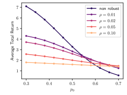
(a) Average Return

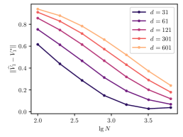
(b) $\|\widehat{V}_{1}-V^{*}_{1}\|$

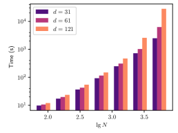
(c) Execution time

Figure 4: Results of RPVI in American Option Experiment. (a) Average total return of different KL radius $\rho$ in the perturbed environments ($N=1000$, $d=61$). (b) Estimation error with different linear function dimension $d$’s and the sizes of dataset $N$’s ($\rho=0.01$). (c) Execution time for different $d$’s, which is shown in log space.

References

- Abbasi-Yadkori et al. (2011) Abbasi-Yadkori, Y., Pál, D., and Szepesvári, C. Improved algorithms for linear stochastic bandits. Advances in neural information processing systems, 24, 2011.
- An et al. (2021) An, G., Moon, S., Kim, J.-H., and Song, H. O. Uncertainty-based offline reinforcement learning with diversified q-ensemble. Advances in neural information processing systems, 34:7436–7447, 2021.
- Badrinath & Kalathil (2021) Badrinath, K. P. and Kalathil, D. Robust reinforcement learning using least squares policy iteration with provable performance guarantees. In International Conference on Machine Learning, pp. 511–520. PMLR, 2021.
- Ben-Tal & Nemirovski (1998) Ben-Tal, A. and Nemirovski, A. Robust convex optimization. Mathematics of operations research, 23(4):769–805, 1998.
- Ben-Tal & Nemirovski (2000) Ben-Tal, A. and Nemirovski, A. Robust solutions of linear programming problems contaminated with uncertain data. Mathematical programming, 88(3):411–424, 2000.
- Bertsekas (2008) Bertsekas, D. P. Approximate dynamic programming. 2008.
- Bertsekas & Tsitsiklis (1995) Bertsekas, D. P. and Tsitsiklis, J. N. Neuro-dynamic programming: an overview. In Proceedings of 1995 34th IEEE conference on decision and control, volume 1, pp. 560–564. IEEE, 1995.
- Bertsimas et al. (2018) Bertsimas, D., Gupta, V., and Kallus, N. Data-driven robust optimization. Mathematical Programming, 167(2):235–292, 2018.
- Chen et al. (2020) Chen, X., Zhou, Z., Wang, Z., Wang, C., Wu, Y., and Ross, K. Bail: Best-action imitation learning for batch deep reinforcement learning. Advances in Neural Information Processing Systems, 33:18353–18363, 2020.
- Cheng et al. (2022) Cheng, C.-A., Xie, T., Jiang, N., and Agarwal, A. Adversarially trained actor critic for offline reinforcement learning. arXiv preprint arXiv:2202.02446, 2022.
- Cox et al. (1979) Cox, J. C., Ross, S. A., and Rubinstein, M. Option pricing: A simplified approach. Journal of financial Economics, 7(3):229–263, 1979.
- Duan et al. (2019) Duan, Y., Ke, T., and Wang, M. State aggregation learning from markov transition data. Advances in Neural Information Processing Systems, 32, 2019.
- Duchi & Namkoong (2021) Duchi, J. C. and Namkoong, H. Learning models with uniform performance via distributionally robust optimization. The Annals of Statistics, 49(3):1378–1406, 2021.
- Duchi et al. (2021) Duchi, J. C., Glynn, P. W., and Namkoong, H. Statistics of robust optimization: A generalized empirical likelihood approach. Mathematics of Operations Research, 46(3):946–969, 2021.
- El Ghaoui & Nilim (2005) El Ghaoui, L. and Nilim, A. Robust solutions to markov decision problems with uncertain transition matrices. Operations Research, 53(5):780–798, 2005.
- Fujimoto & Gu (2021) Fujimoto, S. and Gu, S. S. A minimalist approach to offline reinforcement learning. Advances in neural information processing systems, 34:20132–20145, 2021.
- Fujimoto et al. (2019) Fujimoto, S., Meger, D., and Precup, D. Off-policy deep reinforcement learning without exploration. In International conference on machine learning, pp. 2052–2062. PMLR, 2019.
- Gottesman et al. (2019) Gottesman, O., Johansson, F., Komorowski, M., Faisal, A., Sontag, D., Doshi-Velez, F., and Celi, L. A. Guidelines for reinforcement learning in healthcare. Nature medicine, 25(1):16–18, 2019.
- Goyal & Grand-Clement (2022) Goyal, V. and Grand-Clement, J. Robust markov decision processes: Beyond rectangularity. Mathematics of Operations Research, 2022.
- Ho et al. (2018) Ho, C. P., Petrik, M., and Wiesemann, W. Fast bellman updates for robust mdps. In International Conference on Machine Learning, pp. 1979–1988. PMLR, 2018.
- Ho et al. (2021) Ho, C. P., Petrik, M., and Wiesemann, W. Partial policy iteration for l1-robust markov decision processes. J. Mach. Learn. Res., 22:275–1, 2021.
- Hu & Hong (2013) Hu, Z. and Hong, L. J. Kullback-leibler divergence constrained distributionally robust optimization. Available at Optimization Online, pp. 1695–1724, 2013.
- Huang et al. (2017) Huang, S., Papernot, N., Goodfellow, I., Duan, Y., and Abbeel, P. Adversarial attacks on neural network policies. arXiv preprint arXiv:1702.02284, 2017.
- Iyengar (2005) Iyengar, G. N. Robust dynamic programming. Mathematics of Operations Research, 30(2):257–280, 2005.
- Jiang et al. (2017) Jiang, N., Krishnamurthy, A., Agarwal, A., Langford, J., and Schapire, R. E. Contextual decision processes with low bellman rank are pac-learnable. In International Conference on Machine Learning, pp. 1704–1713. PMLR, 2017.
- Jin et al. (2020) Jin, C., Yang, Z., Wang, Z., and Jordan, M. I. Provably efficient reinforcement learning with linear function approximation. In Conference on Learning Theory, pp. 2137–2143. PMLR, 2020.
- Jin et al. (2021) Jin, Y., Yang, Z., and Wang, Z. Is pessimism provably efficient for offline rl? In International Conference on Machine Learning, pp. 5084–5096. PMLR, 2021.
- Kaufman & Schaefer (2013) Kaufman, D. L. and Schaefer, A. J. Robust modified policy iteration. INFORMS Journal on Computing, 25(3):396–410, 2013.
- Kostrikov et al. (2021) Kostrikov, I., Fergus, R., Tompson, J., and Nachum, O. Offline reinforcement learning with fisher divergence critic regularization. In International Conference on Machine Learning, pp. 5774–5783. PMLR, 2021.
- Kostrikov et al. (2022) Kostrikov, I., Nair, A., and Levine, S. Offline reinforcement learning with implicit q-learning. In International Conference on Learning Representations, 2022.
- Kumar et al. (2019) Kumar, A., Fu, J., Soh, M., Tucker, G., and Levine, S. Stabilizing off-policy q-learning via bootstrapping error reduction. Advances in Neural Information Processing Systems, 32, 2019.
- Kumar et al. (2020) Kumar, A., Zhou, A., Tucker, G., and Levine, S. Conservative q-learning for offline reinforcement learning. Advances in Neural Information Processing Systems, 33:1179–1191, 2020.
- Lange et al. (2012) Lange, S., Gabel, T., and Riedmiller, M. Batch reinforcement learning. In Reinforcement learning, pp. 45–73. Springer, 2012.
- Levine et al. (2020) Levine, S., Kumar, A., Tucker, G., and Fu, J. Offline reinforcement learning: Tutorial, review, and perspectives on open problems. arXiv preprint arXiv:2005.01643, 2020.
- Lim et al. (2013) Lim, S. H., Xu, H., and Mannor, S. Reinforcement learning in robust markov decision processes. Advances in Neural Information Processing Systems, 26, 2013.
- Mannor et al. (2004) Mannor, S., Simester, D., Sun, P., and Tsitsiklis, J. N. Bias and variance in value function estimation. In Proceedings of the twenty-first international conference on Machine learning, pp. 72, 2004.
- Modi et al. (2020) Modi, A., Jiang, N., Tewari, A., and Singh, S. Sample complexity of reinforcement learning using linearly combined model ensembles. In International Conference on Artificial Intelligence and Statistics, pp. 2010–2020. PMLR, 2020.
- Munos & Szepesvári (2008) Munos, R. and Szepesvári, C. Finite-time bounds for fitted value iteration. Journal of Machine Learning Research, 9(5), 2008.
- Namkoong & Duchi (2017) Namkoong, H. and Duchi, J. C. Variance-based regularization with convex objectives. Advances in neural information processing systems, 30, 2017.
- Nilim & El Ghaoui (2005) Nilim, A. and El Ghaoui, L. Robust control of markov decision processes with uncertain transition matrices. Operations Research, 53(5):780–798, 2005.
- Panaganti et al. (2022) Panaganti, K., Xu, Z., Kalathil, D., and Ghavamzadeh, M. Robust reinforcement learning using offline data. arXiv preprint arXiv:2208.05129, 2022.
- Pattanaik et al. (2017) Pattanaik, A., Tang, Z., Liu, S., Bommannan, G., and Chowdhary, G. Robust deep reinforcement learning with adversarial attacks. arXiv preprint arXiv:1712.03632, 2017.
- Pinto et al. (2017) Pinto, L., Davidson, J., Sukthankar, R., and Gupta, A. Robust adversarial reinforcement learning. In International Conference on Machine Learning, pp. 2817–2826. PMLR, 2017.
- Rafailov et al. (2021) Rafailov, R., Yu, T., Rajeswaran, A., and Finn, C. Offline reinforcement learning from images with latent space models. In Learning for Dynamics and Control, pp. 1154–1168. PMLR, 2021.
- Rajeswaran et al. (2016) Rajeswaran, A., Ghotra, S., Ravindran, B., and Levine, S. Epopt: Learning robust neural network policies using model ensembles. arXiv preprint arXiv:1610.01283, 2016.
- Rashidinejad et al. (2021) Rashidinejad, P., Zhu, B., Ma, C., Jiao, J., and Russell, S. Bridging offline reinforcement learning and imitation learning: A tale of pessimism. Advances in Neural Information Processing Systems, 34:11702–11716, 2021.
- Satia & Lave Jr (1973) Satia, J. K. and Lave Jr, R. E. Markovian decision processes with uncertain transition probabilities. Operations Research, 21(3):728–740, 1973.
- Schweitzer & Seidmann (1985) Schweitzer, P. J. and Seidmann, A. Generalized polynomial approximations in markovian decision processes. Journal of mathematical analysis and applications, 110(2):568–582, 1985.
- Shi & Chi (2022) Shi, L. and Chi, Y. Distributionally robust model-based offline reinforcement learning with near-optimal sample complexity. arXiv preprint arXiv:2208.05767, 2022.
- Shi et al. (2021) Shi, T., Chen, D., Chen, K., and Li, Z. Offline reinforcement learning for autonomous driving with safety and exploration enhancement. arXiv preprint arXiv:2110.07067, 2021.
- Siegel et al. (2020) Siegel, N. Y., Springenberg, J. T., Berkenkamp, F., Abdolmaleki, A., Neunert, M., Lampe, T., Hafner, R., Heess, N., and Riedmiller, M. Keep doing what worked: Behavioral modelling priors for offline reinforcement learning. arXiv preprint arXiv:2002.08396, 2020.
- Simester et al. (2006) Simester, D. I., Sun, P., and Tsitsiklis, J. N. Dynamic catalog mailing policies. Management science, 52(5):683–696, 2006.
- Singh et al. (1994) Singh, S., Jaakkola, T., and Jordan, M. Reinforcement learning with soft state aggregation. Advances in neural information processing systems, 7, 1994.
- Tamar et al. (2013) Tamar, A., Xu, H., and Mannor, S. Scaling up robust mdps by reinforcement learning. arXiv preprint arXiv:1306.6189, 2013.
- Tang & Wiens (2021) Tang, S. and Wiens, J. Model selection for offline reinforcement learning: Practical considerations for healthcare settings. In Machine Learning for Healthcare Conference, pp. 2–35. PMLR, 2021.
- Wang et al. (2018) Wang, Q., Xiong, J., Han, L., Liu, H., Zhang, T., et al. Exponentially weighted imitation learning for batched historical data. Advances in Neural Information Processing Systems, 31, 2018.
- Wang et al. (2020) Wang, R., Foster, D. P., and Kakade, S. M. What are the statistical limits of offline rl with linear function approximation? arXiv preprint arXiv:2010.11895, 2020.
- Wang et al. (2021) Wang, Y., Wang, R., Du, S. S., and Krishnamurthy, A. Optimism in reinforcement learning with generalized linear function approximation. In International Conference on Learning Representations, 2021.
- Wiesemann et al. (2013) Wiesemann, W., Kuhn, D., and Rustem, B. Robust markov decision processes. Mathematics of Operations Research, 38(1):153–183, 2013.
- Wu et al. (2019) Wu, Y., Tucker, G., and Nachum, O. Behavior regularized offline reinforcement learning. arXiv preprint arXiv:1911.11361, 2019.
- Wu et al. (2021) Wu, Y., Zhai, S., Srivastava, N., Susskind, J. M., Zhang, J., Salakhutdinov, R., and Goh, H. Uncertainty weighted actor-critic for offline reinforcement learning. In International Conference on Machine Learning, pp. 11319–11328. PMLR, 2021.
- Xie et al. (2021) Xie, T., Cheng, C.-A., Jiang, N., Mineiro, P., and Agarwal, A. Bellman-consistent pessimism for offline reinforcement learning. Advances in neural information processing systems, 34, 2021.
- Xu & Mannor (2010) Xu, H. and Mannor, S. Distributionally robust markov decision processes. Advances in Neural Information Processing Systems, 23, 2010.
- Yang & Wang (2019) Yang, L. and Wang, M. Sample-optimal parametric q-learning using linearly additive features. In International Conference on Machine Learning, pp. 6995–7004. PMLR, 2019.
- Yang et al. (2021a) Yang, W., Zhang, L., and Zhang, Z. Towards theoretical understandings of robust markov decision processes: Sample complexity and asymptotics. arXiv preprint arXiv:2105.03863, 2021a.
- Yang et al. (2021b) Yang, Y., Ma, X., Chenghao, L., Zheng, Z., Zhang, Q., Huang, G., Yang, J., and Zhao, Q. Believe what you see: Implicit constraint approach for offline multi-agent reinforcement learning. Advances in Neural Information Processing Systems, 34:10299–10312, 2021b.
- Yin et al. (2022) Yin, M., Duan, Y., Wang, M., and Wang, Y.-X. Near-optimal offline reinforcement learning with linear representation: Leveraging variance information with pessimism. In International Conference on Learning Representations, 2022.
- Yu et al. (2021) Yu, C., Liu, J., Nemati, S., and Yin, G. Reinforcement learning in healthcare: A survey. ACM Computing Surveys (CSUR), 55(1):1–36, 2021.
- Yu et al. (2018) Yu, F., Xian, W., Chen, Y., Liu, F., Liao, M., Madhavan, V., and Darrell, T. Bdd100k: A diverse driving video database with scalable annotation tooling. arXiv preprint arXiv:1805.04687, 2(5):6, 2018.
- Yu et al. (2020) Yu, T., Thomas, G., Yu, L., Ermon, S., Zou, J. Y., Levine, S., Finn, C., and Ma, T. Mopo: Model-based offline policy optimization. Advances in Neural Information Processing Systems, 33:14129–14142, 2020.
- Yurtsever et al. (2020) Yurtsever, E., Lambert, J., Carballo, A., and Takeda, K. A survey of autonomous driving: Common practices and emerging technologies. IEEE access, 8:58443–58469, 2020.
- Zanette (2021) Zanette, A. Exponential lower bounds for batch reinforcement learning: Batch rl can be exponentially harder than online rl. In International Conference on Machine Learning, pp. 12287–12297. PMLR, 2021.
- Zanette et al. (2020) Zanette, A., Lazaric, A., Kochenderfer, M., and Brunskill, E. Learning near optimal policies with low inherent bellman error. In International Conference on Machine Learning, pp. 10978–10989. PMLR, 2020.
- Zanette et al. (2021) Zanette, A., Wainwright, M. J., and Brunskill, E. Provable benefits of actor-critic methods for offline reinforcement learning. Advances in neural information processing systems, 34:13626–13640, 2021.
- Zhang & Wang (2019) Zhang, A. and Wang, M. Spectral state compression of markov processes. IEEE transactions on information theory, 66(5):3202–3231, 2019.
- Zhang et al. (2020) Zhang, H., Chen, H., Xiao, C., Li, B., Liu, M., Boning, D., and Hsieh, C.-J. Robust deep reinforcement learning against adversarial perturbations on state observations. Advances in Neural Information Processing Systems, 33:21024–21037, 2020.
- Zhou et al. (2021a) Zhou, W., Bajracharya, S., and Held, D. Plas: Latent action space for offline reinforcement learning. In Conference on Robot Learning, pp. 1719–1735. PMLR, 2021a.
- Zhou et al. (2021b) Zhou, Z., Zhou, Z., Bai, Q., Qiu, L., Blanchet, J., and Glynn, P. Finite-sample regret bound for distributionally robust offline tabular reinforcement learning. In International Conference on Artificial Intelligence and Statistics, pp. 3331–3339. PMLR, 2021b.