Distribution Calibration for Out-of-Domain Detection with Bayesian Approximation

Abstract

Out-of-Domain (OOD) detection is a key component in a task-oriented dialog system, which aims to identify whether a query falls outside the predefined supported intent set. Previous softmax-based detection algorithms are proved to be overconfident for OOD samples. In this paper, we analyze overconfident OOD comes from distribution uncertainty due to the mismatch between the training and test distributions, which makes the model can’t confidently make predictions thus probably causing abnormal softmax scores. We propose a Bayesian OOD detection framework to calibrate distribution uncertainty using Monte-Carlo Dropout. Our method is flexible and easily pluggable into existing softmax-based baselines and gains 33.33% OOD F1 improvements with increasing only 0.41% inference time compared to MSP. Further analyses show the effectiveness of Bayesian learning for OOD detection.

1 Introduction

Detecting Out-of-Domain (OOD) or unknown intents from user queries is key for a task-oriented dialog system Gnewuch et al. (2017); Akasaki and Kaji (2017); Tulshan and Dhage (2018); Shum et al. (2018); Zeng et al. (2021a, b); Wu et al. (2022). It aims to know when a user query falls outside their range of predefined supported intents to avoid performing wrong operations. Different from normal intent classification tasks, lack of labeled OOD examples leads to poor prior knowledge about these unknown intents, making it challenging to detect OOD samples.

A rich line of OOD intent detection algorithms has been developed recently, among which softmax-based methods demonstrated promise Guo et al. (2017); Liang et al. (2018); Zheng et al. (2020). Softmax-based methods leverage softmax outputs extracted from an in-domain (IND) intent model and operate under the assumption that the test OOD samples get a lower likelihood probability than the ID data. For example, Maximum Softmax Probability (MSP) Hendrycks and Gimpel (2017) detects a test query as OOD if its max softmax probability is lower than a fixed threshold. However, all these models make a strong distributional assumption of the practical OOD probability being uniform, which has been proven wrong because neural networks can produce over-confidently high softmax scores even for OOD samples Guo et al. (2017). Therefore, solving the overconfidence issue is still challenging for OOD detection.

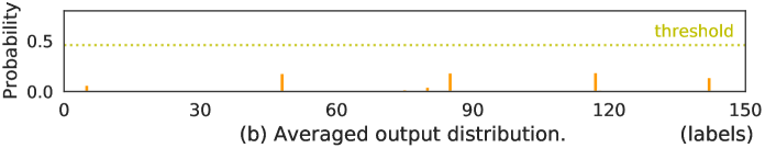
Figure 1: Multiple predicted probability distributions of an OOD sample under different random seeds. We train four identical models on the same data but only use different random seeds. Fig (a) displays each output distribution of an OOD input and Fig (b) shows the averaged output distribution.

In this paper, we study the overconfidence issue from the perspective of Bayesian learning Gal and Ghahramani (2016). Essentially, the reason for overconfidence is that a model cannot confidently make predictions on the input OOD utterances (unknow-unknow) due to the lack of prior knowledge of OOD data. In other words, even given the same input OOD intent, the predicted probability distributions using different random seeds are completely different, uniform, sharp, or any distribution. Fig 1 show an example. We find models with different initialization seeds can output diverse distributions for OOD input, maybe cause overconfidence in several in-domain classes. But the averaged output is close to a uniform distribution. We also find models with different seeds are more robust to IND input and obtain consistent outputs (see Appendix C.2). Therefore, one direct way to solve the distribution uncertainty is to train multiple models independently and assemble their outputs for the final result. But this method is not applicable to practical scenarios for large training cost. In this paper, we propose a Bayesian OOD detection framework to calibrate distribution uncertainty. Specifically, we firstly train an in-domain intent classifier using IND data, then in the test stage, we perform multiple stochastic forward passes with a certain dropout rate (like 0.7) and average the output normalized logits as a final probability. Without increasing any new parameters, we calibrate distribution uncertainty by tending to expectation uniform distribution via Monte-Carlo Dropout Gal and Ghahramani (2016). Our method can be easily extended to existing softmax-based OOD detection methods and gain significant OOD improvements with only increasing little inference time compared to baselines, even outperform the state-of-the-art distance-based methods like LOF Lin and Xu (2019) and GDA Xu et al. (2020). Our contributions are two-fold: (1) We analyze the intrinsic reason of overconfidence issue via distribution uncertainty and propose a Bayesian OOD detection framework to calibrate this uncertainty using Monte-Carlo Dropout. (2) We provide theoretical and empirical analysis to demonstrate the effectiveness of our Bayesian OOD method.

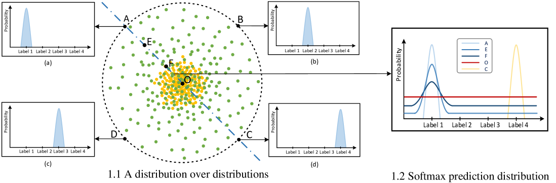
Figure 2: A distribution over distributions where each dot represents a softmax prediction distribution for a test OOD sample and all the dots denote a distribution over distributions. We also display softmax prediction distributions of several dots on the dot line in Fig 1.2.

2 Method

2.1 Understanding OOD Detection

Problem Definition We refer to training data $D$ as IND data. We aim to detect the input utterances $x$ belonging to OOD and correctly classify the utterances belonging to IND utilizing a well-calibrated classifier trained only on finite IND data $D$.

The predictive uncertainty of a classification model $P(\upsilon|x,D)$ is commonly divided into data uncertainty (aleatoric), distribution uncertainty and model uncertainty (epistemic)Kiureghian and Ditlevsen (2009); Malinin and Gales (2018):

$$P(\upsilon|x,D)=\iint{\underbrace{P(\upsilon|\mu)}_{\text{data}}\underbrace{P(\mu|x,\theta)}_{\text{distribution}}\underbrace{P(\theta|D)}_{\text{model}}d\mu\!\,d\theta}$$ (1)

The model uncertainty is described by the posterior distribution over model parameters $\theta$, and it can be lowered by increasing the amount of data and simplifying the model complexity. The data uncertainty is described by the posterior distribution over classes, where $\upsilon$ is the predicted distribution of all possible in-domain intent classes for OOD detection. It arises from the natural complexity of the data, such as class overlap, label noise and homoscedastic noise. It is a property of the world, and cannot be changed. The distribution uncertainty is modeled with a distribution over distribution, where $\mu$ is the categorical distribution over simplex. It arises due to the mismatch between the training and test distributions. We give an example in Fig 2 which displays a distribution over distributions on a simplex (Dirichlet distribution Malinin and Gales (2018)) where each dot represents a softmax prediction distribution for a test OOD sample and all the dots denote a distribution over distributions. For an input utterance $x$, softmax-based detection algorithms like MSP assume that the distribution of OOD utterances ($v_{ood}$) should be very close to the uniform distribution (the yellow dots in Fig 2) and the distribution of IND utterances ($v_{ind}$) should be very close to one-hot distribution (e.g. Fig 2(a)-(d)). However, the practical OOD samples (green dots) exactly yield a sparse distribution over the simplex where each OOD sample may get a sharp softmax prediction distribution (like one-hot distribution) or a flat softmax prediction distribution (like uniform distribution). Due to the lack of prior knowledge of OOD data, the model cannot confidently make predictions on the input OOD utterances (unknow-unknow) which is the essential reason why the predicted probability distributions of the same OOD sample are completely different under different random seeds and even get very high max softmax scores (Fig 1). In other words, distribution uncertainty could lead to overconfidence in the prediction of OOD samples.

Therefore, how to alleviate the distribution uncertainty is the key to solving the overconfidence problem in OOD detection.

2.2 Bayesian Approximation

In order to alleviate the distribution uncertainty, we consider marginalizing out $\theta$ in Eq 1:

$$P(\upsilon|x,D)=\int{P(\upsilon|\mu)P(\mu|x,D)d\mu}\vspace{-0.09cm}$$ (2)

This yields expected estimates of data and distributional uncertainty given model uncertainty. Marginalization is intractable in deep neural networks, thus we consider using $q(\omega)$ to approximate the intractable posterior though Monte-Carlo Sampling algorithm Tsymbalov et al. (2020); Gal and Ghahramani (2016):

$$P(\upsilon|x,D)=\int{P(\upsilon|\omega)q(\omega)d\omega}$$ (3)

where $\omega=\{W_{i}\}_{i=1}^{l}$ is the random variables for a model with $l$ layers. We define $q(\omega)$ as:

$$W_{i}=M_{i}\cdot diag(\,\![\alpha_{i,j}\!\,]_{i=1}^{k_{i}})$$ (4)

$$\alpha_{i,j}\sim Bernoulli(p_{i})$$ (5)

Where $p_{i}$ and $M_{i}$ are the variational parameters. The binary variable $\alpha_{i,j}$ indicates whether unit $j$ of the $i-1$ layer will be passed to the next layer. Specifically, we sample $N$ sets of independent random vectors of realisations from the Bernoulli distribution $\{\alpha_{1}^{n},...,\alpha_{l}^{n}\}_{n=1}^{N}$ with $\![\alpha_{i,j}\!]_{i=1}^{k_{i}}$ giving $\{W_{1}^{n},...,W_{L}^{n}\}_{n=1}^{N}$. Then we average the output:

$$E_{q(\upsilon|x,D)}\!(\upsilon\!)\approx\frac{1}{N}\sum_{n=1}^{N}\hat{\upsilon}{(x,D,W_{1}^{n},...,W_{l}^{n})}$$ (6)

According to the Law of Large Numbers Yao and Gao (2016), when N is large enough, the predicted distribution will converge in expected uniform distribution. That is, we can calibrate the practical sparse OOD distribution (green dots) over the simplex into ideal dense OOD distribution (yellow dots) by Bayesian approximation to mitigate the overconfidence issue, which is verified in the following empirical experiments.

2.3 OOD Detection with Bayesian Learning

Fig 3(a) shows the overall architecture of our proposed OOD detection model. The part in the dashed box is a well-trained feature extractor based on Bi-LSTM Hochreiter and Schmidhuber (1997) or BERT Devlin et al. (2019). It is trained on labeled in-domain data using cross-entropy loss. Fig 3(b) shows the Bayesian approximation process for distribution calibration. We adopt Monte-Carlo Dropout and average the output normalized logits from multiple stochastic forward passes: $\boldsymbol{\bar{v}}=\frac{1}{N}\sum_{i=1}^{N}\boldsymbol{v_{i}}$. In this way, we calibrate the softmax distribution to the expected distribution, which close to a uniform distribution. Then, we apply two softmax-based metrics for OOD detection, which is $m_{MSP}=\max(\boldsymbol{\bar{v}})$ and $m_{Entropy}=-\sum_{i=1}^{c}\bar{v}_{i}\log\bar{v}_{i}$. We further apply a empirical threshold to distinguish IND and OOD data.

Model		CLINC-Full				CLINC-Imbal
		OOD		IND		OOD		IND
		F1	Recall	F1	ACC	F1	Recall	F1	ACC
LSTM	LOF Lin and Xu (2019)	59.28	58.32	86.08	85.87	55.37	51.03	80.51	82.79
	GDA Xu et al. (2020)	65.79	64.14	87.90	86.83	61.38	63.80	85.35	84.20
	MSP Hendrycks and Gimpel (2017)	50.13	45.60	87.73	87.25	44.93	41.10	84.96	84.16
	MSP+Bayes.(ours)	70.05	68.38	88.91	88.57	61.70	57.50	85.92	85.65
	Entropy Zheng et al. (2020)	68.05	67.96	88.97	88.68	64.45	63.80	86.07	85.71
	Entropy+Bayes.(ours)	72.02	71.70	89.10	88.73	68.32	67.61	86.34	86.11
BERT	MSP	52.79	50.50	87.81	87.46	48.76	46.70	85.87	85.65
	MSP+Bayes.(ours)	71.25	69.58	89.10	89.56	64.32	62.00	86.39	85.87
	Entropy	68.97	68.83	89.13	88.72	65.25	64.89	86.21	85.94
	Entropy+Bayes.(ours)	72.85	72.42	89.47	88.94	69.11	68.49	86.74	86.42

Table 1: Performance comparison between our method and baselines on CLINC-Full and CLINC-Imbal datasets (p <0.01). Bayes. represents our proposed Bayesian approximation via Monte-Carlo Dropout.

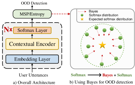
Figure 3: The overall architecture of our method.

3 Experiments

3.1 Datasets

CLINC	Full	Imbal
Avg utterance length	9	9
Intents	150	150
Training set size	15100	10625
Training samples per class	100	25/50/75/100
Training OOD samples amount	100	100
Development set size	3100	3100
Development samples per class	20	20
Development OOD samples amount	100	100
Testing Set Size	5500	5500
Testing samples per class	30	30
Development OOD samples amount	1000	1000

Table 2: Statistics of the CLINC datasets.

We perform experiments on two public benchmark OOD datasets, CLINC-Full and CLINC-Imbal Larson et al. (2019). We show the detailed statistic of these datasets in Table 2. They both contain 150 in-domain intents across 10 domains. The only difference is that, for CLINC-Imbal, there are either 25, 50, 75 or 100 training queries per in-scope intent, rather than 100. Note that all the datasets we used have a fixed set of labeled OOD data but we don’t use it for training.

3.2 Metrics

We report both OOD metrics: Recall and F1-score(F1) and in-domain metrics: F1-score(F1) and Accuracy(ACC). Since we aim to improve the performance of detecting out-of-domain intents from user queries, OOD Recall and F1 are the main evaluation metrics in this paper.

3.3 Baselines

For detection algorithms, we use LOF, GDA, MSP and Entropy, none of them need OOD supervised training. For the feature extractor, we use LSTM and BERT. We provide a more comprehensive comparison and implementation details of these models in the Appendix.

3.4 Main Results

Table 1 shows our main results on two benchmarks. Our Bayesian method significantly outperforms softmax-based baselines including MSP and Entropy, even distance-based SOTA GDA on OOD metrics. Specifically, on CLINC-Full, Bayes improves 19.92% and 3.97% OOD F1 compared to MSP and Entropy using LSTM, which proves MSP suffers from severe overconfidence and our method helps calibrate OOD distribution. The performance gap between MSP and Entropy is because Entropy based on softmax output distribution can better capture distinguished information for OOD than MSP based on a single value of softmax distribution. We find similar improvements under the BERT setting on CLINIC-Imbal dataset.

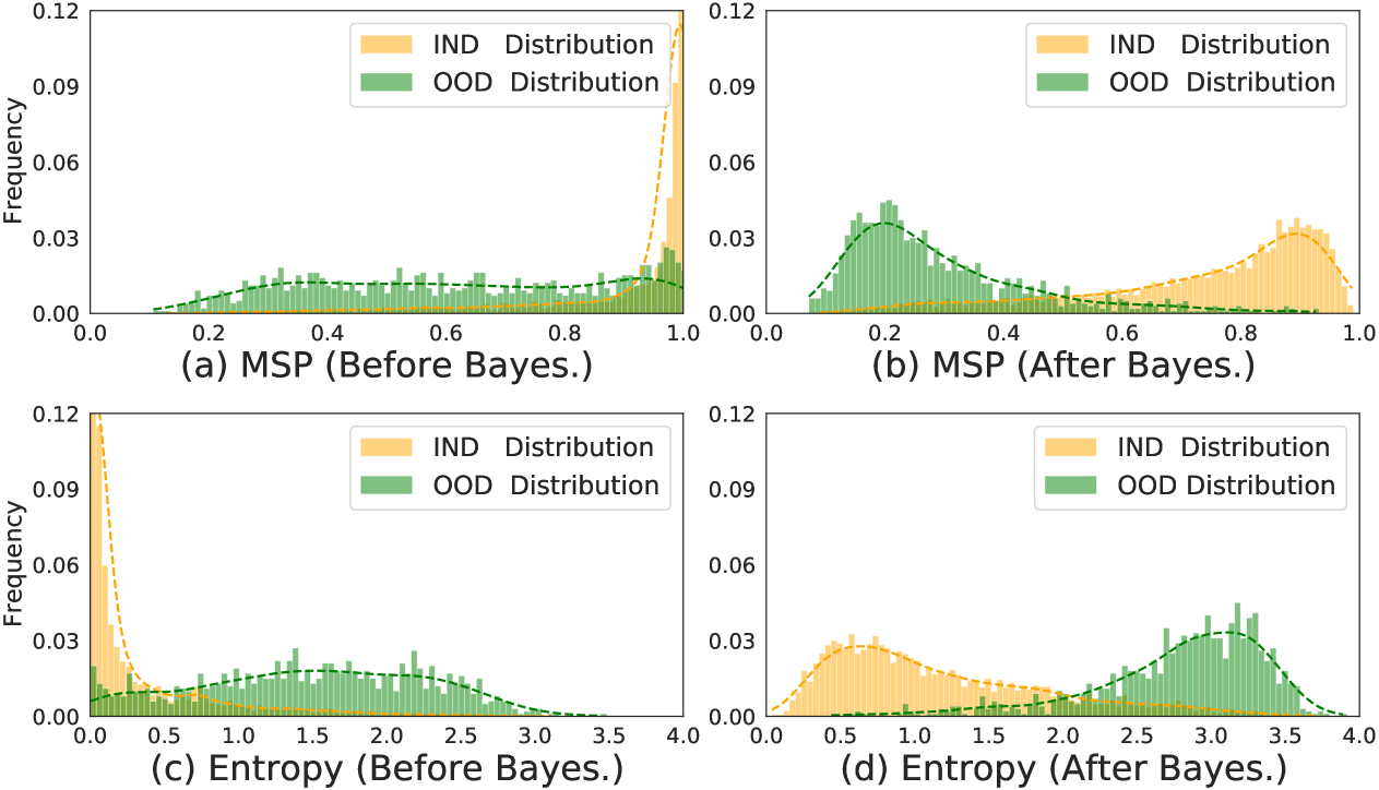
Figure 4: Effect of Bayesian approximation on MSP and Entropy confidence distributions of IND and OOD.

4 Analysis

4.1 Effect of Bayesian approximation

Fig 4 shows the MSP and Entropy confidence distributions of IND and OOD test data using Bayesian to verify the effect of our method. Due to the over-confidence issue of OOD, we find IND and OOD curves overlap a lot in the original confidence scores. The overlapping part of Entropy is less, which confirms its better OOD detection performance. After calibration using Bayes, the overlap part of both methods is reduced, making it easier to distinguish between IND and OOD.

4.2 Analysis of Distribution Calibration

Table 3 shows the effect of Bayes on OOD Dirichlet Distribution. We calculate the KL-divergence between the predicted averaged softmax distribution and the uniform distribution of each test OOD sample and report the mean and median values on the whole test set. With the increase of sampling, we observe a larger drop on OOD mean and median KL values than INDs. It proves that Bayes can gradually calibrate the $v_{ood}$ to a uniform distribution and thus make the sparse OOD Dirichlet distribution dense but not affect IND. Besides, we find N = 100 already achieves good performance to reduce inference cost. We provide an efficiency comparison in Section 4.3 and find 33.33% OOD F1 improvements only increase 0.41% time.

4.3 Analysis of Cost-effectiveness

We show the comparison between the time consumption and the corresponding performance improvement in Table 4 on CLINC-Full which has 15100 training data and 5500 test data. We find that when the number of samples N is 10, our method can improve the performance by 33.33% while only increasing the time by 0.41%, which proves that our proposed method is very cost-effective. Besides, we also find that more sampling times lead to more improvements, demonstrating that more accurate calibration significantly boosts OOD detection. In terms of time consumption and performance improvement, N = 100 is the most appropriate sampling parameter. When the sampling time is 1000, the cost-effectiveness is not as high as when $N=10$. We consider that methods such as model distillation and pruning can reduce the time consumption, and we will leave it to future work. In general, we can choose the appropriate number of samples according to the computing resources.

$\lg$ $N$	Statistical Indicators
	OOD		IND
	mean	median	mean	median
0	3.63	3.60	4.74	4.95
1	2.59	2.47	4.36	4.58
2	2.27	2.15	4.31	4.54
3	2.24	2.12	4.30	4.54

Table 3: KL-divergence between predicted distribution and uniform distribution on CLINC-Full. The smaller value is better for OOD. $N$ is the number of dropout.

lgN	Time(s)	OOD F1	Increased
			Time(%)	OOD F1(%)
0	240.00	50.13	-	-
1	240.98	66.84	$\uparrow$ 0.41	$\uparrow$ 33.33
2	252.41	70.05	$\uparrow$ 5.17	$\uparrow$ 39.74
3	388.36	70.82	$\uparrow$ 61.82	$\uparrow$ 41.27

Table 4: Time consumption and corresponding performance improvement of Bayesian approximation based MSP.

4.4 Analysis of Parameters

Table 5 reports the OOD F1 under different dropout probability and sampling times. Within a range between 0.3 to 0.7, the larger dropout probability leads to better OOD detection performance. This is because OOD data is more vulnerable to feature loss and its averaged softmax prediction distribution tends to be more uniform. Besides, more sampling times lead to improvements, demonstrating that more accurate calibration significantly boosts OOD detection. We also find that the performance on p=0.7, N=10 is better than the performance on p=0.3, N=1000. This prompts us to choose a higher p (e.g. 0.7), which can effectively reduce the time consumption (1000->10). In addition, OOD F1 is not sensitive to excessive sampling times.

$\lg$ $N$	Dropout Probability
	0.3	0.4	0.5	0.6	0.7	0.8
1	57.21	60.97	61.80	64.27	66.84	64.01
2	60.78	64.38	65.84	68.87	70.05	69.03
3	63.32	65.35	67.51	69.33	70.82	69.69

Table 5: Effect of Bayesian approximation with different parameters on OOD F1-score.

5 Conclusion

In this paper, we conduct an analysis of why previous softmax-based detection algorithms like MSP or Entropy suffer from the overconfidence issue. We find OOD samples exactly yield a sparse distribution over the simplex and evenly distribute over the whole space. Therefore, we propose a simple but strong Bayesian approximation method to calibrate OOD distribution. Experiments prove the effectiveness of our method. We hope to provide new guidance for future OOD detection work.

Appendix A Baseline Details

We compare many types of unsupervised OOD detection models. For detection algorithms, we use LOF(Local Outlier Factor)Lin and Xu (2019), GDA(Gaussian Discriminant Analysis)Xu et al. (2020), MSP(Maximum Softmax Probability)Hendrycks and Gimpel (2017) and Entropy. For feature extractor, we use LSTM(Long Short Term Memory)Hochreiter and Schmidhuber (1997) and BERT(Bidirectional Encoder Representations from Transformers)Devlin et al. (2019).

MSP (Maximum Softmax Probability)Hendrycks and Gimpel (2017) uses maximum softmax probability as the confidence score and regards an intent as OOD if the score is below a fixed threshold.

LOF (Local Outlier Factor)Lin and Xu (2019) A detecting unknown intents in the utterance algorithm with local density. It Assumes that unknown intents’ local density is significantly lower than its k-nearest neighbor’s.

GDA (Gaussian Discriminant Analysis) Xu et al. (2020) A generative distance-based classifier for OOD detection with Euclidian space. For avoiding over-confidence problems, they estimate the class-conditional distribution on feature spaces of DNNs via Gaussian discriminant analysis. GDA is the state-of-the-art detection method till now, our proposed method using Bayesian approximation still significantly outperforms GDA. We also compare our method on two feature extractors for further study.

LSTM (Long Short Term Memory)Hochreiter and Schmidhuber (1997) A neural network that was proposed with the motivation of an analysis of Recurrent Neural Nets, which found that long time lags were inaccessible to existing architectures because backpropagated error either blows up or decays exponentially.

BERT (Bidirectional Encoder Representations from Transformers)Devlin et al. (2019) A neural network that is trained to predict elided words in the text and then fine-tuned on our data. Note that they both trained only on labeled in-domain data using cross-entropy loss.

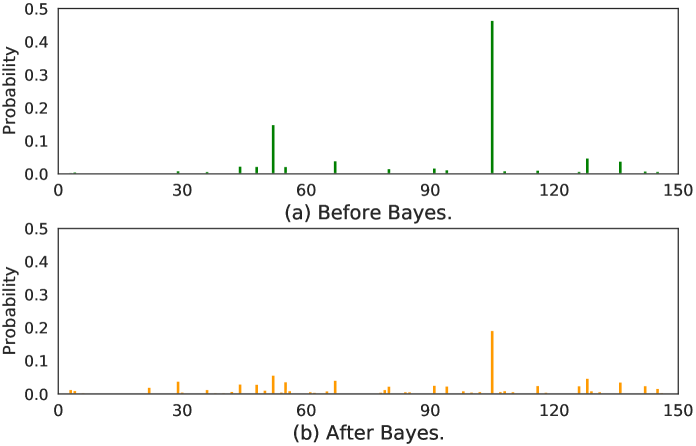
Figure 5: Effect of Bayesian approximation on softmax distribution of OOD sample.

Appendix B Implementation Details

We use the public pre-trained 300 dimensions GloVe embeddings Pennington et al. (2014) or bert-base-uncased Devlin et al. (2019) model to embed tokens. We use a two-layer BiLSTM as a feature extractor and set the dimension of hidden states to 128. We use Adam optimizer Kingma and Ba (2014) to train our model. We set a learning rate to 1E-03 for GloVe+LSTM and 1E-04 for BERT. In the training stage, We set the dropout probability to 0.5 and set the training epoch up to 200 with an early stop. We train only on in-domain labeled data. We use the best F1 scores on the validation set to calculate the detection method’s threshold adaptively. For our proposed Bayesian approximation, we set the dropout probability to 0.7, and the dropout sampling times to 100. Each result of the experiments is tested 10 times under the same setting and gets the average value. The training stage of our model lasts about 4 minutes using GloVe embeddings, and 12 minutes using Bert-base-uncased, both on a single Tesla T4 GPU(16 GB of memory). The average value of the trainable model parameters is 3.05M. We will release our code after blind review.

Appendix C Visualization of softmax prediction distribution.

C.1 Visualization of OOD samples

In Fig 5, we give a 150-dimensional class distribution of an OOD sample to help understand our calibration process. The upper part of the figure is the distribution obtained by using the primary feature extractor. The softmax prediction distribution has obvious over-confidence in a particular IND category. The lower half of the figure presents the distribution after calibration by Bayesian approximation, which is flatter and meets the expectations of the OOD sample. When applying softmax-based detection methods, the latter will more easily recognized as OOD.

C.2 Visualization of IND samples

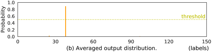
Figure 6: Multiple predicted probability distributions of an IND sample under different random seeds.

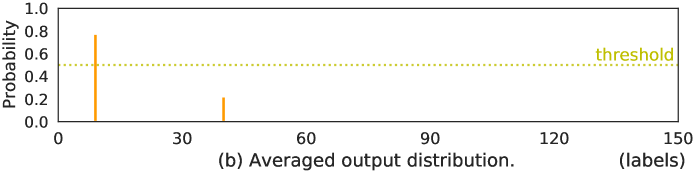
Figure 7: Multiple predicted probability distributions of an IND sample under different random seeds.

Corresponding to Fig 1, Fig 6 and Fig 7 show predicted probability distributions of two IND sample under different random seeds over 150 classes. We train four identical models on the same data but only use different random seeds. Fig (a) displays each output distribution of an IND input and Fig (b) shows the averaged output distribution. Specifically, Fig 6 shows when the input utterance is ’block my american saving bank for now’, the model obtains the maximum prediction probability on ground truth (freeze_account) under four random seeds and averaged output. Specifically, The maximum probabilities of prediction are 0.77, 0.96, 0.90 and 0.84 under different random seeds, and 0.87 under averaged output. In the experiments, we find that most IND samples present the state of Fig 6, that is, under different random samples setting, the model is very confident to give the input IND utterances with high confidence probability in the ground-truth category. We guess that this is because the model has seen some IND data in the training phase, and is familiar with IND classification, that is, the distribution uncertainty of IND is not serious. We also show another example in Fig 7 which the input utterance is ’where is improve the credit score’ and the corresponding true label is improve_credit_score. However, we find that under one random sampling setting, the model mispredicts into credit_score category with a probability of 0.61. We argue this is due to the fact that the two are easily confused with each other. Under this random sampling parameter setting, the model has not learned the feature ability to accurately distinguish these two categories. In addition, we also find that although there are wrong predictions, most of the IND predictions are accurate and have a high prediction probability, so that the highest prediction probability can still be obtained on the ground-truth label after averaging the distributions. This also reveals that our method will not damage the performance of IND classification, and can even avoid misjudgment among some confusing IND categories.

References

- Akasaki and Kaji (2017) Satoshi Akasaki and Nobuhiro Kaji. 2017. Chat detection in an intelligent assistant: Combining task-oriented and non-task-oriented spoken dialogue systems. ArXiv, abs/1705.00746.
- Devlin et al. (2019) Jacob Devlin, Ming-Wei Chang, Kenton Lee, and Kristina Toutanova. 2019. BERT: Pre-training of deep bidirectional transformers for language understanding. In Proceedings of the 2019 Conference of the North American Chapter of the Association for Computational Linguistics: Human Language Technologies, Volume 1 (Long and Short Papers), pages 4171–4186, Minneapolis, Minnesota. Association for Computational Linguistics.
- Gal and Ghahramani (2016) Yarin Gal and Zoubin Ghahramani. 2016. Dropout as a bayesian approximation: Representing model uncertainty in deep learning. In Proceedings of The 33rd International Conference on Machine Learning, volume 48 of Proceedings of Machine Learning Research, pages 1050–1059, New York, New York, USA. PMLR.
- Gnewuch et al. (2017) Ulrich Gnewuch, S. Morana, and A. Maedche. 2017. Towards designing cooperative and social conversational agents for customer service. In International Conference on Information Systems.
- Guo et al. (2017) Chuan Guo, Geoff Pleiss, Yu Sun, and Kilian Q Weinberger. 2017. On calibration of modern neural networks. In International Conference on Machine Learning, pages 1321–1330. PMLR.
- Hendrycks and Gimpel (2017) Dan Hendrycks and Kevin Gimpel. 2017. A baseline for detecting misclassified and out-of-distribution examples in neural networks. ArXiv, abs/1610.02136.
- Hochreiter and Schmidhuber (1997) S. Hochreiter and J. Schmidhuber. 1997. Long short-term memory. Neural Computation, 9:1735–1780.
- Kingma and Ba (2014) Diederik P Kingma and Jimmy Ba. 2014. Adam: A method for stochastic optimization. arXiv preprint arXiv:1412.6980.
- Kiureghian and Ditlevsen (2009) Armen Der Kiureghian and O. Ditlevsen. 2009. Aleatory or epistemic? does it matter? Structural Safety, 31:105–112.
- Larson et al. (2019) Stefan Larson, Anish Mahendran, Joseph J. Peper, Christopher Clarke, Andrew Lee, Parker Hill, Jonathan K. Kummerfeld, Kevin Leach, Michael A. Laurenzano, Lingjia Tang, and Jason Mars. 2019. An evaluation dataset for intent classification and out-of-scope prediction. In Proceedings of the 2019 Conference on Empirical Methods in Natural Language Processing and the 9th International Joint Conference on Natural Language Processing (EMNLP-IJCNLP).
- Liang et al. (2018) Shiyu Liang, Yixuan Li, and R. Srikant. 2018. Enhancing the reliability of out-of-distribution image detection in neural networks. arXiv: Learning.
- Lin and Xu (2019) Ting-En Lin and Hua Xu. 2019. Deep unknown intent detection with margin loss. In Proceedings of the 57th Annual Meeting of the Association for Computational Linguistics, pages 5491–5496.
- Malinin and Gales (2018) A. Malinin and M. Gales. 2018. Predictive uncertainty estimation via prior networks. In Proceedings of the 32nd International Conference on Neural Information Processing Systems, page 7047–7058.
- Pennington et al. (2014) Jeffrey Pennington, Richard Socher, and Christopher D Manning. 2014. Glove: Global vectors for word representation. In Proceedings of the 2014 conference on empirical methods in natural language processing (EMNLP), pages 1532–1543.
- Shum et al. (2018) H. Shum, X. He, and Di Li. 2018. From eliza to xiaoice: challenges and opportunities with social chatbots. Frontiers of Information Technology & Electronic Engineering, 19:10–26.
- Tsymbalov et al. (2020) Evgenii Tsymbalov, K. Fedyanin, and Maxim Panov. 2020. Dropout strikes back: Improved uncertainty estimation via diversity sampled implicit ensembles. ArXiv, abs/2003.03274.
- Tulshan and Dhage (2018) Amrita S Tulshan and Sudhir Namdeorao Dhage. 2018. Survey on virtual assistant: Google assistant, siri, cortana, alexa. In International symposium on signal processing and intelligent recognition systems, pages 190–201.
- Wu et al. (2022) Yanan Wu, Keqing He, Yuanmeng Yan, QiXiang Gao, Zhiyuan Zeng, Fujia Zheng, Lulu Zhao, Huixing Jiang, Wei Wu, and Weiran Xu. 2022. Revisit overconfidence for OOD detection: Reassigned contrastive learning with adaptive class-dependent threshold. In Proceedings of the 2022 Conference of the North American Chapter of the Association for Computational Linguistics: Human Language Technologies, pages 4165–4179, Seattle, United States. Association for Computational Linguistics.
- Xu et al. (2020) Hong Xu, Keqing He, Yuanmeng Yan, Sihong Liu, Zijun Liu, and Weiran Xu. 2020. A deep generative distance-based classifier for out-of-domain detection with mahalanobis space. In Proceedings of the 28th International Conference on Computational Linguistics, pages 1452–1460, Barcelona, Spain (Online). International Committee on Computational Linguistics.
- Yao and Gao (2016) Kai Yao and Jinwu Gao. 2016. Law of large numbers for uncertain random variables. IEEE Transactions on Fuzzy Systems, 24:615–621.
- Zeng et al. (2021a) Zhiyuan Zeng, Keqing He, Yuanmeng Yan, Zijun Liu, Yanan Wu, Hong Xu, Huixing Jiang, and Weiran Xu. 2021a. Modeling discriminative representations for out-of-domain detection with supervised contrastive learning. In Proceedings of the 59th Annual Meeting of the Association for Computational Linguistics and the 11th International Joint Conference on Natural Language Processing (Volume 2: Short Papers), pages 870–878, Online. Association for Computational Linguistics.
- Zeng et al. (2021b) Zhiyuan Zeng, Keqing He, Yuanmeng Yan, Hong Xu, and Weiran Xu. 2021b. Adversarial self-supervised learning for out-of-domain detection. In Proceedings of the 2021 Conference of the North American Chapter of the Association for Computational Linguistics: Human Language Technologies, pages 5631–5639, Online. Association for Computational Linguistics.
- Zheng et al. (2020) Yinhe Zheng, Guanyi Chen, and Minlie Huang. 2020. Out-of-domain detection for natural language understanding in dialog systems. IEEE/ACM Transactions on Audio, Speech, and Language Processing, 28:1198–1209.