Combining Metric Learning and Attention Heads For Accurate and Efficient Multilabel Image Classification

Abstract

Multi-label image classification allows predicting a set of labels from a given image. Unlike multiclass classification, where only one label per image is assigned, such a setup is applicable for a broader range of applications. In this work we revisit two popular approaches to multilabel classification: transformer-based heads and labels relations information graph processing branches. Although transformer-based heads are considered to achieve better results than graph-based branches, we argue that with the proper training strategy, graph-based methods can demonstrate just a small accuracy drop, while spending less computational resources on inference. In our training strategy, instead of Asymmetric Loss (ASL), which is the de-facto standard for multilabel classification, we introduce its metric learning modification. In each binary classification sub-problem it operates with $L_{2}$ normalized feature vectors coming from a backbone and enforces angles between the normalized representations of positive and negative samples to be as large as possible. This results in providing a better discrimination ability, than binary cross entropy loss does on unnormalized features. With the proposed loss and training strategy, we obtain SOTA results among single modality methods on widespread multilabel classification benchmarks such as MS-COCO, PASCAL-VOC, NUS-Wide and Visual Genome 500. Source code of our method is available as a part of the OpenVINO™ Training Extensions.

1 INTRODUCTION

Starting from the impressive AlexNet [Krizhevsky et al., 2012] breakthrough on the ImageNet benchmark [Deng et al., 2009], the deep-learning era has drastically changed approaches to almost every computer vision task. Throughout this process multiclass classification problem was a polygon for developing new architectures [He et al., 2016, Howard et al., 2019, Tan and Le, 2019] and learning paradigms [Chen et al., 2020, Khosla et al., 2020, He et al., 2019a]. At the same time, multilabel classification has been developing not so intensively, although the presence of several labels on one image is more natural, than having one hard label. Due to a lack of specialized multilabel datasets, researchers turned general object detection datasets such as MS-COCO [Lin et al., 2014] and PASCAL VOC [Everingham et al., 2009] into challenging multilabel classification benchmarks by removing bounding boxes from the data annotation and leveraging only their class labels.

Despite the recent progress in solving the mentioned benchmarks, the latest works focus mainly on the resulting model accuracy, not taking into account computational complexity [Liu et al., 2021] or the use of outdated training techniques [Chen et al., 2019], introducing promising model architectures at the same time.

In this work, we are revisiting the latest approaches to multilabel classification, to propose a lightweight solution suitable for real-time applications and also improve the performance-accuracy tradeoff of the existing models.

The main contributions of this paper are as follows:

• We proposed a modification of ML-GCN [Chen et al., 2019] that adds graph attention operations [Veličković et al., 2018] and performs graph and CNN features fusion in a more conventional way than generating a set of binary classifiers in the graph branch.

• We demonstrated that using a proper training strategy, one can decrease the performance gap between transformer-based heads and label co occurrence modeling via graph attention.

• We first applied the metric learning paradigm to multilabel a classification task and proposed a modified version of angular margin binary loss [Wen et al., 2021], which adds an ASL [Baruch et al., 2021] mechanism to it.

• We verified the effectiveness of our loss and overall training strategy with comprehensive experiments on widespread multilabel classification benchmarks: PASCAL VOC, MS-COCO, Visual Genome [Krishna et al., 2016] and NUS-WIDE [Chua et al., 2009].

2 RELATED WORK

Historically, multilabel classification was attracting less attention than the multiclass scenario, but nonetheless there is still great progress in that field. Notable progress was achieved by developing advanced loss functions [Baruch et al., 2021], label co occurrence modeling [Chen et al., 2019, Yuan et al., 2022], designing advanced classification heads [Liu et al., 2021, Ridnik et al., 2021b, Zhu and Wu, 2021] and discovering architectures taking into account spatial distribution of objects via exploring attentional regions [Wang et al., 2017, Gao and Zhou, 2021].

Conventionally, a multilabel classification task is transformed into a set of binary classification tasks, which are solved by optimizing a binary cross-entropy loss function. Each single-class classification subtask suffers from a hard positives-negatives imbalance. The more classes the training dataset contains, the more negatives we have in each of the single-class subtasks, because an image typically contains a tiny fraction of the vast number of all classes. A modified asymmetric loss [Baruch et al., 2021], that down weights and hard-thresholds easy negative samples, showed impressive results, reaching state-of-the-art results on multiple popular multi-label datasets without any sophisticated architecture tricks. These results indicate that a proper choice of a loss function is crucial for multilabel classification performance.

Another promising direction is designing class-specific classifiers instead of using a fully connected layer on top of a single feature vector produced by a backbone network. This approach also doesn’t introduce additional training steps and marginally increases model complexity. Authors of [Zhu and Wu, 2021] propose a drop-in replacement of the global average pooling layer that generates class-specific features for every category. Leveraging compact transformer heads for generating such features [Liu et al., 2021, Ridnik et al., 2021b] turned out to be even more effective. This approach assumes pooling class-specific features by employing learnable embedding queries.

Considering the distribution of objects locations, or statistical label relationships requires data pre-processing and additional assumptions [Chen et al., 2019, Yuan et al., 2022] or sophisticated model architecture [Wang et al., 2017, Gao and Zhou, 2021]. For instance, [Chen et al., 2019, Yuan et al., 2022] represents labels by word embeddings; then a directed graph is built over these label representations, where each node denotes a label. Then stacked GCNs are learned over this graph to obtain a set of object classifiers. The method relies on an ability to represent labels as words, which is not always possible. Spatial distribution modeling requires placing a RCNN-like [Girshick et al., 2014] module inside the model [Wang et al., 2017, Gao and Zhou, 2021], which drastically increases the complexity of the training pipeline.

3 METHOD

In this section, we describe the overall training pipeline and details of our approach. We aimed not only to achieve competitive results, but also to make the training more friendly to the end user and adaptive to data. Thus, following the principles described in [Prokofiev and Sovrasov, 2022], we use lightweight model architectures, hyperparameters optimization and early stopping.

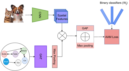
Figure 1: Overall diagram of the proposed GAT-based feature reweighting approach. Features obtained from the label relations graph by applying GAT are used to reweight channels in the CNN spatial features. Later, a pooling operation is applied to the reweighted features to obtain a vector representation. Finally, the resulting vectors are fed into binary classifiers $W_{j}$ and optimized with the AAM loss, which is introduced in this work.

3.1 Model architecture

We chose EfficientNetV2 [Tan and Le, 2021] and TResNet [Ridnik et al., 2021a] as base architectures for performing multilabel image classification. Namely, we conducted all the experiments on TResNet-L, EfficientNetV2 small, and large. On top of these backbones, we used two different features aggregation approaches and compared their effectiveness and performance.

3.2 Transformer multilabel classification head

As a representer of transformer-based feature aggregation methods, we use the ML-Decoder [Ridnik et al., 2021b] head. It provides up to $K$ feature vectors (where $K$ is the number of classes) as a model output instead of a single class-agnostic vector when using a standard global average pooling (GAP) head. Let’s denote $x\in\mathbb{R}^{C\times H\times W}$ as a model input, then the model $F$ with parameters $W$ produces a downscaled multi-channel featuremap $f=F_{W}(x)\in\mathbb{R}^{S\times\frac{H}{d}\times\frac{W}{d}}$, where $S$ is the number of output channels, $d$ is the spatial downscale factor. That featuremap is then passed to the ML-Decoder head: $v=MLD(f)\in\mathbb{R}^{M\times L}$, where $M$ is the embedding dimension, $L\leq K$ is the number of groups in decoder. Finally, vectors $v$ are projected to $K$ class logits by a fully-connected (if $L=K$) or group fully-connected projection (if $L<K$) as it is described in [Ridnik et al., 2021b]. In our experiments we set $L=\min(100,K)$. Also, we $L_{2}$ normalize the arguments of all dot products in projections in case if we need to attach a metric learning loss to the ML-Decoder head.

3.3 Graph attention multilabel branch

The original structure of the graph processing branch from [Chen et al., 2019] supposes generating classifiers right in this branch and then applying them directly to the features generated by a backbone. This approach is incompatible with the transformer-based head or any other processing of the raw spatial features $f$, like CSRA [Zhu and Wu, 2021]. To alleviate this limitation, we propose the architecture shown in Figure 1.

First, we generate the label correlation matrix $Z\in\mathbb{R}^{K\times K}$ in the same way as in [Chen et al., 2019]. Together with the word embeddings $G\in\mathbb{R}^{K\times N}$, obtained with GLOVE [Makarenkov et al., 2016] model, where $N=300$ is word embeddings dimension, we utilize $Z$ as an input of the Graph Attention Network [Veličković et al., 2018]. Unlike [Yuan et al., 2022], we use estimations of conditional probabilities to build $Z$, rather than fully relying on GLOVE and calculating cosine similarities.

We process the input with the graph attention layers and obtain output $h\in\mathbb{R}^{S\times K}$. Then we derive the most influential features through the max pooling operation and receive the weights $w\in\mathbb{R}^{S}$ for further re-weighting of the CNN spatial features: $\tilde{f}=w\bigodot f$. Next, we apply global average pooling and max-pooling operations to $\tilde{f}$ in parallel, sum the results and obtain the final latent embedding $\tilde{v}\in\mathbb{R}^{S}$. The embedding $\tilde{v}$ is finally passed to the binary classifiers. Instead of applying a simple spatial pooling, we can pass the weighted features $\tilde{f}$ to the ML-Decoder or any other features processing module.

The main advantage of using the graph attention (GAT) branch for features re-weighting over the transformer head is a tiny computational and model complexity overhead at the inference stage. Since the GAT branch has the same input for any image, we can compute the result of its execution only once, before starting the inference of the resulting model. At the same time, the GAT requires a vector representation of labels. Such representations can be generated by a text-to-vec model in case we have a meaningful description for all labels (even single word ones). This condition doesn’t always hold: some datasets could have untitled labels. How to generate representations for labels in that case is still an open question.

3.4 Angular margin binary classification

Recently, asymmetric loss [Baruch et al., 2021] has become a standard loss option for performing multilabel classification. By design it penalizes each logit with a modified binary cross-entropy loss. Asymmetric handling of positives and negatives allows ASL to down-weight the negative part of the loss to tackle the positives-negatives imbalance problem. But this approach leaves a room for improvement from the model’s discriminative ability perspective.

Angular margin losses are known for generating more discriminative classification features than the cross-entropy loss, which is a must-have property for recognition tasks [Deng et al., 2018, Wen et al., 2021, Sovrasov and Sidnev, 2021].

We propose joining paradigms from [Baruch et al., 2021] and [Wen et al., 2021] to build even stronger loss for multilabel classification. Denote the result of the dot product between the normalized class embedding $v_{j}$ produced by ML-Decoder ($v_{j}=\tilde{v},\>j=\overline{1,K}$ if we use a backbone alone or with an optional GAT-based head) and the $j$-th binary classifier $W_{j}$ as $cos\Theta_{j}$. Then, for a training sample $x$ and corresponding embeddings set $v$ we formulate our asymmetric angular margin loss (AAM) as:

$$L_{AAM}(v,y)=-\sum_{j=1}^{K}L_{j}(cos\Theta_{j},y)$$

$$L_{j}(cos\Theta_{j},y)=\frac{k}{s}yp_{-}^{\gamma^{-}}\log{p_{+}}+\frac{1-k}{s}(1-y)p_{+}^{\gamma^{+}}\log{p_{-}},\\$$ (1)

$$p_{+}=\sigma{(s(cos\Theta_{j}-m))},$$

$$p_{-}=\sigma{(-s(cos\Theta_{j}+m))},$$

where $s$ is a scale parameter, $m$ is an angular margin, $k$ is negative-positive weighting coefficient, $\gamma^{+}$ and $\gamma^{-}$ are weighting parameters from ASL. Despite the large number of hyperparameters, some of them could be safely fixed (like $\gamma^{+}$ and $\gamma^{-}$ from ASL). The effect of varying $s$ saturates when increasing $s$ (see Figure 2b), and if the suitable value of this parameter is large enough, we don’t need to tune it precisely. Also, values of $m$ should be close to $0$, because it duplicates to some extent the effect of $s$ and $\gamma$ and can even bring undesirable increase of the negative part of AAM (see Figure 2a). Detailed analysis of the hyperparameters is provided in Section 4.5.

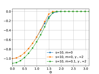
(a) Loss for $p_{-}$

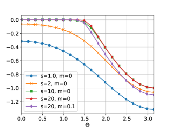
(b) Loss for $p_{+}$

Figure 2: Plots of positive and negative parts of AAM with varying hyperparameters

3.5 Details of the training strategy

As in our former work [Prokofiev and Sovrasov, 2022], we aim to make the training pipeline for multilabel classification reliable, fast and adaptive to dataset, so we use the following components:

• SAM [Foret et al., 2020] optimizer with no bias decay [He et al., 2019b] is a default optimizer;

• EMA weights averaging for an additional protection from overfitting;

• Initial learning rate estimation process from [Prokofiev and Sovrasov, 2022];

• OneCycle [Smith, 2018] learning rate scheduler;

• Early stopping heuristic: if the best result on the validation subset hasn’t been improved during 5 epochs, and evaluation results stay below the EMA averaged sequence of the previous best results, the training process stops;

• Random flip, pre-defined Randaugment [Cubuk et al., 2020] strategy and Cutout [Devries and Taylor, 2017] data augmentations.

4 EXPERIMENTS

In this section, we conduct a comparison of our approach with the state-of-the-art solutions on popular multilabel benchmarks. Besides the mAP metric, we present the GFLOPs for each method to consider the speed/accuracy trade-off. Also, we show the results of the ablation study to reveal the importance of each training pipeline component.

4.1 Datasets

To compare the performance of different methods, we picked up widespread datasets for multilabel classification that are listed in Table 1. According to the table, all of them have a noticeable positives-negatives imbalance on each image: the average number of presented labels per image is significantly lower than the number of classes.

Also, we use a precisely annotated subset of OpenImages V6 [Kuznetsova et al., 2018] for pre-training purposes. We join the original training and testing parts into one training subset and use the original validation subset for testing.

Table 1: Image classification datasets which were used for training.

Dataset	# of classes	# of Images		Avg # of
		Train	Validation	labels per image
Pascal VOC 2007 [Everingham et al., 2009]	20	5011	4952	1.58
MS-COCO 2014 [Lin et al., 2014]	80	117266	4952	2.92
NUS-WIDE [Chua et al., 2009]	81	119103	50720	2.43
Visual Genome 500 [Krishna et al., 2016]	500	82904	10000	13.61
OpenImages V6 [Kuznetsova et al., 2018]	601	1866950	41151	5.23

4.2 Evaluation protocol

We adopt commonly used metrics for evaluation of multilabel classification models: mean average precision (mAP) over all categories, overall precision (OP), recall (OR), F1-measure (OF1) and per category precision (CP), recall (CR), F1-measure (CF1). We use the mAP as a main metric; others are provided when an advanced comparison of approaches is conducted. In every operation where confidence thresholding is required, threshold 0.5 is substituted. The exact formulas of the mentioned metrics can be found in [Liu et al., 2021].

4.3 Pretraining

Although the multilabel classification task is similar to multiclass classification, a multilabel model should pay attention to several objects on an image, instead of concentrating its attention on one object. Thus, additional task-specific pre-training on a large-scale dataset looks beneficial to standard ImageNet pre-training, and it was shown in recent works [Ridnik et al., 2021b]. In this work we utilize OpenImages V6 for pretraining. According to our experiments, the precisely-annotated subset containing 1.8M images is enough to get a substantial improvement over the ImageNet weights.

To obtain pretrained weights on OpenImages for our models, we use the ML-Decoder head, $224\times 224$ input resolution, ASL loss with $\gamma^{+}=0$ and $\gamma^{-}=7$, learning rate $0.001$, and 50 epochs of training with OneCycle scheduler.

For TResNet-L we use the weights provided with the source code in [Ridnik et al., 2021b].

4.4 Comparison with the state-of-the-art

In all cases where we use EfficientNet-V2-s as a backbone we also use our training strategy from Section 3.5 for a fair comparison. For ASL loss [Baruch et al., 2021] we set $lr=0.0001$, $\gamma^{-}=4$, $\gamma^{+}=0$ as suggested in the original paper [Baruch et al., 2021]. We share the following hyperparameters across all the experiments: $m=0.0$, $k=0.7$, EMA decay factor equals to $0.9997$, $\rho=0.05$ for the SAM optimizer. Other hyperperameters for particular datasets were found empirically or via coarse grid search.

In Table 2 results on MS-COCO are presented. For this dataset we set $s=23$, $lr=0.007$, $\gamma^{-}=1$, $\gamma^{+}=0$. With our AAM loss, we can achieve a state-of-the-art result using TResNet-L as a backbone. At the same time, the combination of EfficientNetV2-s with ML-Decoder and AAM loss outperforms TResNet-L with ASL, while consuming 3.5x less FLOPS. GCN/GAT branches perform slightly worse than ML-Decoder, but still improves results over EfficientNetV2-s + ASL with a marginal computational cost at inference.

Table 2: Comparison with the state-of-the-art on MS-COCO dataset.

Method	Backbone	Input resolution	mAP	GFLOPs
ASL [Baruch et al., 2021]	TResNet-L	448x448	88.40	43.50
Q2L [Liu et al., 2021]	TResNet-L	448x448	89.20	60.40
GATN [Yuan et al., 2022]	ResNeXt-101	448x448	89.30	36.00
Q2L [Liu et al., 2021]	TResNet-L	640x640	90.30	119.69
ML-Decoder [Ridnik et al., 2021b]	TResNet-L	448x448	90.00	36.15
ML-Decoder [Ridnik et al., 2021b]	TResNet-L	640x640	91.10	73.42
ASL∗	EfficientNet-V2-s	448x448	87.05	10.83
ML-GCN∗	EfficientNet-V2-s	448x448	87.50	10.83
Q2L∗	EfficientNet-V2-s	448x448	87.35	16.25
ML-Decoder∗	EfficientNet-V2-s	448x448	88.25	12.28
GAT re-weighting (ours)	EfficientNet-V2-s	448x448	87.70	10.83
GAT re-weighting (ours)	TResNet-L	448x448	89.95	35.20
ML-Decoder + AAM (ours)	EfficientNet-V2-s	448x448	88.75	12.28
ML-Decoder + AAM (ours)	EfficientNet-V2-L	448x448	90.10	49.92
ML-Decoder + AAM (ours)	TResNet-L	448x448	90.30	36.15
ML-Decoder + AAM (ours)	TResNet-L	640x640	91.30	73.42
∗Trained by us using our training strategy

Results on Pascal-VOC can be found in Table 3. We set $s=17$, $lr=0.005$, $\gamma^{-}=2$, $\gamma^{+}=1$ to train our models on this dataset. Our modification of the GAT branch outperforms ML-Decoder when using EfficientNet-V2-s, while AAM loss gives a small performance boost and allows achieving SOTA with TResNet-L. Also, on Pascal-VOC EfficientNet-V2-s with all of the considered additional graph branches or heads demonstrates a great speed/accuracy trade-off outperforming TResNet-L with ASL.

Table 3: Comparison with the state-of-the-art on Pascal-VOC dataset.

Method	Backbone	Input resolution	mAP	GFLOPs
ASL [Baruch et al., 2021]	TResNet-L	448x448	94.60	43.50
Q2L [Liu et al., 2021]	TResNet-L	448x448	96.10	57.43
GATN [Yuan et al., 2022]	ResNeXt-101	448x448	96.30	36.00
ML-Decoder [Ridnik et al., 2021b]	TResNet-L	448x448	96.60	35.78
ASL∗	EfficientNet-V2-s	448x448	94.24	10.83
Q2L∗	EfficientNet-V2-s	448x448	94.94	15.40
ML-GCN∗	EfficientNet-V2-s	448x448	95.25	10.83
ML-Decoder∗	EfficientNet-V2-s	448x448	95.54	12.00
GAT re-weighting (ours)	EfficientNet-V2-s	448x448	96.00	10.83
GAT re-weighting (ours)	TResNet-L	448x448	96.67	35.20
ML-Decoder + AAM (ours)	EfficientNet-V2-s	448x448	95.86	12.00
ML-Decoder + AAM (ours)	EfficientNet-V2-L	448x448	96.05	49.92
ML-Decoder + AAM (ours)	TResNet-L	448x448	96.70	35.78
∗Trained by us using our training strategy

Tables 4 and 5 show results on NUS and VG500 datasets. For NUS dataset we set $s=23$, $lr=0.009$, $\gamma^{-}=2$, $\gamma^{+}=1$. For VG500 the hyperparameters are $s=25$, $lr=0.005$, $\gamma^{-}=1$, $\gamma^{+}=0$. ML-Decoder clearly outperforms GCN and GAT branches on NUS-WIDE dataset. Also on NUS EfficientNet-V2-s with the AAM loss and GAT or ML-decoder head performs significantly better than the original implementations of Q2L and ASL with TResNet-L.

On VG500 we don’t provide results of applying GCN or GAT branches, because this dataset has unnamed labels, so we can not apply a text-to-vec model to generate representations of graph nodes. Applying AAM with ML-Decoder on VG500 together with increased resolution allows achieving SOTA performance on this dataset as well.

As a result of the experiments, we can conclude that the combination of ML-Decoder with AAM loss gives an optimal performance on all of the considered datasets, while using the GAT-based branch could lead to better inference speed at the price of a small accuracy drop. In particular, EfficientNetV2-s model with the GAT-based head or ML-Decoder on top outperforms T-ResNet-L with ASL, while consuming at least 3.5x less FLOPS. These results enable real-time applications of high-accuracy multilabel classification models on edge devices with a small computational budget. At the same time, applying AAM loss, ML-Decoder and carefully designed training strategy allows achieving SOTA-level accuracy with TResNet-L.

Table 4: Comparison with the state-of-the-art on NUS-WIDE.

Method	Backbone	Input resolution	mAP	GFLOPs
GATN [Yuan et al., 2022]	ResNeXt-101	448x448	59.80	36.00
ASL [Baruch et al., 2021]	TResNet-L	448x448	65.20	43.50
Q2L [Liu et al., 2021]	TResNet-L	448x448	66.30	60.40
ML-GCN∗	EfficientNet-V2-s	448x448	66.30	10.83
ASL∗	EfficientNet-V2-s	448x448	65.20	10.83
Q2L∗	EfficientNet-V2-s	448x448	65.79	16.25
ML-Decoder∗	EfficientNet-V2-s	448x448	67.07	12.28
GAT re-weighting (ours)	EfficientNet-V2-s	448x448	66.85	10.83
GAT re-weighting (ours)	TResNet-L	448x448	68.10	35.20
ML-Decoder + AAM (ours)	EfficientNet-V2-s	448x448	67.60	12.28
ML-Decoder + AAM (ours)	TResNet-L	448x448	68.30	36.16
∗Trained by us using our training strategy

Table 5: Comparison with the state-of-the-art on VG500.

Method	Backbone	Input resolution	mAP	GFLOPs
C-Tran [Lanchantin et al., 2021]	ResNet101	576x576	38.40	-
Q2L [Liu et al., 2021]	TResNet-L	512x512	42.50	119.37
ASL∗	EfficientNet-V2-s	576x576	38.84	17.90
Q2L∗	EfficientNet-V2-s	576x576	40.35	32.81
ML-Decoder∗	EfficientNet-V2-s	576x576	41.20	20.16
ML-Decoder + AAM (ours)	EfficientNet-V2-s	576x576	42.00	20.16
ML-Decoder + AAM (ours)	TResNet-L	576x576	43.10	59.63
∗Trained by us using our training strategy

4.5 Ablation study

To demonstrate the impact of each component on the whole pipeline, we add them to a baseline one by one. As a baseline we take EfficientNetV2-s backbone and ASL loss with SGD optimizer. We set all the hyper parameters of the ASL loss and learning rate as in [Baruch et al., 2021]. We use the training strategy described in Section 3.5 for all the experiments.

In Table 6 we can see that each component brings an improvement, except adding the GAT branch. ML Decoder has enough capacity to learn labels correlation information, so further cues, that provide the GAT branch, don’t improve the result. Also, we can see that tuning of the $\gamma$ parameters is beneficial for the AAM loss, but the metric learning approach itself brings an improvement even without it. Finally, adding the GAT branch to ML-Decoder doesn’t increase the accuracy, indicating that additional information, coming from GAT, gives no new cues to ML-Decoder.

Table 6: Algorithm’s components contribution.

Method	P-VOC	COCO	N-WIDE	VG500
baseline	93.58	85.90	63.85	37.85
+ SAM	94.00	86.75	65.20	38.50
+ OI wghts	94.24	87.05	65.54	38.84
+ MLD	95.54	88.30	67.07	41.20
+ AM loss∗	95.80	88.60	67.30	41.90
+ AAM	95.86	88.75	67.60	42.00
+ GAT	95.85	88.70	67.20	-
∗ AAM with $\gamma+=\gamma-=0$

5 CONCLUSION

In this work, we revisited two popular approaches to multilabel classification: transformer-based heads and labels graph branches. We refined the performance of these approaches by applying our training strategy with the modern bag of tricks and introducing a novel loss for multilabel classification called AAM. The loss combines properties of the ASL loss and metric learning approach and allows achieving competitive results on popular multilabel benchmarks. Although we demonstrated that graph branches perform very close to transformer-based heads, there is one major drawback of the graph-based method: it relies on labels’ representations provided by a language model. The direction of future work could be developing an approach which would build a label relations graph relying on representations extracted directly from images, not involving potentially meaningless label names.

6 SUPPLEMENTARY MATERIALS

6.1 Extended ablation study

6.1.1 Hyperparameters impact

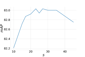
(a) COCO

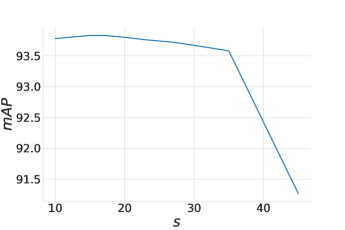
(b) VOC

Figure 3: The performance curves of EfficientNetV2-s+MLD+AAM model with different values of the $s$ parameter. Margin parameter in AAM loss is set to zero. Training resolution is 224x224.

Figure 3 shows the scale parameter $s$ impact on the training pipeline. We fix margin parameter at 0.0 value. We use our full training pipeline with AAM loss and ML-Decoder on 224x224 resolution for faster training. We can conclude that the value of $s$ is correlated with the number of classes. For a small number of classes, the optimal value lies in the range 10-20. Otherwise, the 20-30 range will be a good choice.

Figure 4 shows margin influence from AAM loss. We see that this parameter brings unnecessary complexity to the choice of extra hyperparameter. We can exclude this parameter and simplify applying of the loss function.

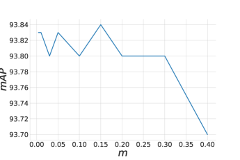
(a) VOC

(b) COCO

Figure 4: The performance curves of EfficientNetV2-s+MLD+AAM model with different values of the $m$ parameter. We fixed other hyperparameters for each dataset for all experiments. Training resolution is 224x224.

Table 7 shows the impact of the different asymmetry parameters values $\gamma^{+}$ and $\gamma^{-}$. As the authors of ASL [Baruch et al., 2021] state in their work, a larger $\gamma^{-}$ is required to handle a larger positive-negative imbalance. They also set $\gamma^{+}$ to 0 for all experiments, but we observe that there are datasets where non-zero $\gamma^{+}$ in AAM loss could bring an improvement as well.

We also notice that in the case of AAM loss, we need just 0-2 values ranges, as we have additional global loss scale parameter $\frac{1-k}{s}$ in (1).

Table 7: Asymmetry influence on the training pipeline.

Gamma	VOC-2007	COCO	NUS-WIDE	VG500
$\gamma^{-}$ = 0, $\gamma^{+}$ = 0	95.80	88.60	67.20	41.90
$\gamma^{-}$ = 1, $\gamma^{+}$ = 0	95.80	88.75	67.30	42.00
$\gamma^{-}$ = 2, $\gamma^{+}$ = 0	95.77	88.68	67.47	41.90
$\gamma^{-}$ = 3, $\gamma^{+}$ = 0	95.78	88.62	67.27	41.80
$\gamma^{-}$ = 2, $\gamma^{+}$ = 1	95.86	88.64	67.60	41.95
$\gamma^{-}$ = 3, $\gamma^{+}$ = 1	95.80	88.52	67.60	41.60

6.1.2 Graph attention branch and transformer head comparison

Table 8: Comparison of GAN vs GCN method and ML Decoder.

Step	VOC-2007	COCO	NUS-WIDE
ML-GCN EfficientNetV2-s	95.25	87.50	66.30
GAN re-weighting EfficientNetV2-s	96.00	87.70	66.85
EfficientNetV2-s + MLD	95.86	88.75	67.60
GAN re-weighting EfficientNetV2-s + MLD	95.85	88.70	67.20

Table 9: Comparison of graph-based method and transformer based in low resolution setup.

Step	VOC-2007	COCO	NUS-WIDE
EfficientNetV2-s	92.85	82.25	65.60
GAN re-weighting EfficientNetV2-s	93.15	82.55	65.87
EfficientNetV2-s + MLD	93.77	83.03	66.74
GAN re-weighting EfficientNetV2-s + MLD	93.71	83.03	66.60

In this section we compare our proposed new re-weighting scheme and the GCN method. If we refer to ML-GCN work [Chen et al., 2019], we see that the training strategy the authors chose for their method is rather simple. We argue that if we add a modern bag of training tricks to the method, the accuracy potentially could increase. We train backbone with ML-GCN head as described in [Chen et al., 2019], but with our training strategy as described in Section 3.5. Table 8 shows that GAN with a re-weighting scheme is more sophisticated in incorporating inter-label correlation. At the same time, the global attention ability of the transformer is sufficient for seeking internal dependencies. Even if we combine two methods and add to the model apriori information about the conditional probability of appearing labels, we will not obtain better quality.

The next point is to check the ability of the transformer and GAN model to handle case of the high level of label noise. A high level of label noise can be achieved by simply reducing the image resolution. Most of the small objects (especially in COCO and NUS-WIDE datasets) will disappear because of resize artifacts.

Table 9 shows the obtained results on all data with resolution 224x224. We also present the results of the model without both ML Decoder and GAN. We can conclude, that despite the fact that GAN branch is sufficient to help the ordinary model to obtain global information on label distribution and co-occurrence, the transformer-based head can derive this information implicitly from the CNN features in a more efficient way. Again, adding GAN as an additional branch doesn’t improve the results.

6.2 Confidence threshold tuning

Conventionally, threshold a value equals to $0.5$ is used for calculating OP, OR, OF1 and CP, CR, CF1. But to apply a classification model in the wild under the variety of input data and presented classes, one need to estimate per-class confidence thresholds. When we don’t have an access to the target real-world data, we can at least take into account per-class threshold variance, which arises because of training data distribution and loss function modifications. To do that, we propose finding per class thresholds by maximizing F1 score on each class via grid search on the train subset. Then we can evaluate the obtained thresholds on the validation subset and check if the precision-recall balance was improved.

Table 10: Results of confidence thresholds calibration for EfficientNetV2-s+MLD model trained with AAM.

Dataset	OF1	OF1-adapt	CF1	CF1-adapt
P-VOC	91.14	91.94	92.60	93.21
COCO	82.86	84.39	85.03	86.06
N-WIDE	71.88	75.52	72.90	75.04
VG500	56.04	54.09	55.15	53.07

In Table 10 the results of thresholds tuning for EfficientNetV2-s model trained with AAM loss on several datasets are shown. Precision-recall balance was improved by the mentioned procedure under train-validation distribution shift conditions for all of the considered datasets excepting Visual Genome 500. There thresholds tuning on train slightly decreased both OF1 and CF1 scores. This fact indicates that VG500 has a big distribution gap between the train and validation subsets, which the model can’t handle (mAP $<50\%$). Thus, if the trained model has low accuracy, estimating confidence threshold on the training subset may not work as expected.

REFERENCES

- Baruch et al., 2021 Baruch, E. B., Ridnik, T., Zamir, N., Noy, A., Friedman, I., Protter, M., and Zelnik-Manor, L. (2021). Asymmetric loss for multi-label classification. ICCV.
- Chen et al., 2020 Chen, T., Kornblith, S., Norouzi, M., and Hinton, G. (2020). A simple framework for contrastive learning of visual representations. arXiv preprint arXiv:2002.05709.
- Chen et al., 2019 Chen, Z.-M., Wei, X.-S., Wang, P., and Guo, Y. (2019). Multi-label image recognition with graph convolutional networks. CVPR.
- Chua et al., 2009 Chua, T.-S., Tang, J., Hong, R., Li, H., Luo, Z., and Zheng, Y. (2009). Nus-wide: a real-world web image database from national university of singapore. In CIVR.
- Cubuk et al., 2020 Cubuk, E. D., Zoph, B., Shlens, J., and Le, Q. (2020). Randaugment: Practical automated data augmentation with a reduced search space. In Advances in Neural Information Processing Systems, volume 33, pages 18613–18624.
- Deng et al., 2009 Deng, J., Dong, W., Socher, R., Li, L.-J., Li, K., and Fei-Fei, L. (2009). ImageNet: A Large-Scale Hierarchical Image Database. In CVPR09.
- Deng et al., 2018 Deng, J., Guo, J., and Zafeiriou, S. (2018). Arcface: Additive angular margin loss for deep face recognition. ArXiv.
- Devries and Taylor, 2017 Devries, T. and Taylor, G. W. (2017). Improved regularization of convolutional neural networks with cutout. ArXiv, abs/1708.04552.
- Everingham et al., 2009 Everingham, M., Gool, L. V., Williams, C. K. I., Winn, J. M., and Zisserman, A. (2009). The pascal visual object classes (voc) challenge. International Journal of Computer Vision, 88.
- Foret et al., 2020 Foret, P., Kleiner, A., Mobahi, H., and Neyshabur, B. (2020). Sharpness-aware minimization for efficiently improving generalization. ArXiv, abs/2010.01412.
- Gao and Zhou, 2021 Gao, B.-B. and Zhou, H.-Y. (2021). Learning to discover multi-class attentional regions for multi-label image recognition. IEEE Transactions on Image Processing, 30:5920–5932.
- Girshick et al., 2014 Girshick, R. B., Donahue, J., Darrell, T., and Malik, J. (2014). Rich feature hierarchies for accurate object detection and semantic segmentation. CVPR.
- He et al., 2019a He, K., Fan, H., Wu, Y., Xie, S., and Girshick, R. (2019a). Momentum contrast for unsupervised visual representation learning. arXiv preprint arXiv:1911.05722.
- He et al., 2016 He, K., Zhang, X., Ren, S., and Sun, J. (2016). Deep residual learning for image recognition. CVPR.
- He et al., 2019b He, T., Zhang, Z., Zhang, H., Zhang, Z., Xie, J., and Li, M. (2019b). Bag of tricks for image classification with convolutional neural networks. In CVPR.
- Howard et al., 2019 Howard, A. G., Sandler, M., Chu, G., Chen, L.-C., Chen, B., Tan, M., Wang, W., Zhu, Y., Pang, R., Vasudevan, V., Le, Q. V., and Adam, H. (2019). Searching for mobilenetv3. ICCV.
- Khosla et al., 2020 Khosla, P., Teterwak, P., Wang, C., Sarna, A., Tian, Y., Isola, P., Maschinot, A., Liu, C., and Krishnan, D. (2020). Supervised contrastive learning. In Advances in Neural Information Processing Systems, volume 33, pages 18661–18673.
- Krishna et al., 2016 Krishna, R., Zhu, Y., Groth, O., Johnson, J., Hata, K., Kravitz, J., Chen, S., Kalantidis, Y., Li, L.-J., Shamma, D. A., Bernstein, M. S., and Fei-Fei, L. (2016). Visual genome: Connecting language and vision using crowdsourced dense image annotations. International Journal of Computer Vision, 123:32–73.
- Krizhevsky et al., 2012 Krizhevsky, A., Sutskever, I., and Hinton, G. E. (2012). Imagenet classification with deep convolutional neural networks. In Advances in Neural Information Processing Systems 25, pages 1097–1105.
- Kuznetsova et al., 2018 Kuznetsova, A., Rom, H., Alldrin, N. G., Uijlings, J. R. R., Krasin, I., Pont-Tuset, J., Kamali, S., Popov, S., Malloci, M., Duerig, T., and Ferrari, V. (2018). Dataset v 4 unified image classification , object detection , and visual relationship detection at scale.
- Lanchantin et al., 2021 Lanchantin, J., Wang, T., Ordonez, V., and Qi, Y. (2021). General multi-label image classification with transformers. CVPR.
- Lin et al., 2014 Lin, T.-Y., Maire, M., Belongie, S. J., Hays, J., Perona, P., Ramanan, D., Dollár, P., and Zitnick, C. L. (2014). Microsoft coco: Common objects in context. In ECCV.
- Liu et al., 2021 Liu, S., Zhang, L., Yang, X., Su, H., and Zhu, J. (2021). Query2label: A simple transformer way to multi-label classification. ArXiv, abs/2107.10834.
- Makarenkov et al., 2016 Makarenkov, V., Shapira, B., and Rokach, L. (2016). Language models with pre-trained (glove) word embeddings. arXiv: Computation and Language.
- Prokofiev and Sovrasov, 2022 Prokofiev, K. and Sovrasov, V. (2022). Towards efficient and data agnostic image classification training pipeline for embedded systems. In ICIAP.
- Ridnik et al., 2021a Ridnik, T., Lawen, H., Noy, A., and Friedman, I. (2021a). Tresnet: High performance gpu-dedicated architecture. WACV.
- Ridnik et al., 2021b Ridnik, T., Sharir, G., Ben-Cohen, A., Ben-Baruch, E., and Noy, A. (2021b). Ml-decoder: Scalable and versatile classification head.
- Smith, 2018 Smith, L. N. (2018). A disciplined approach to neural network hyper-parameters: Part 1 - learning rate, batch size, momentum, and weight decay. ArXiv, abs/1803.09820.
- Sovrasov and Sidnev, 2021 Sovrasov, V. and Sidnev, D. (2021). Building computationally efficient and well-generalizing person re-identification models with metric learning. ICPR.
- Tan and Le, 2019 Tan, M. and Le, Q. V. (2019). Efficientnet: Rethinking model scaling for convolutional neural networks. ArXiv, abs/1905.11946.
- Tan and Le, 2021 Tan, M. and Le, Q. V. (2021). Efficientnetv2: Smaller models and faster training. ArXiv, abs/2104.00298.
- Veličković et al., 2018 Veličković, P., Cucurull, G., Casanova, A., Romero, A., Liò, P., and Bengio, Y. (2018). Graph Attention Networks. ICLR.
- Wang et al., 2017 Wang, Z., Chen, T., Li, G., Xu, R., and Lin, L. (2017). Multi-label image recognition by recurrently discovering attentional regions. ICCV.
- Wen et al., 2021 Wen, Y., Liu, W., Weller, A., Raj, B., and Singh, R. (2021). Sphereface2: Binary classification is all you need for deep face recognition. ArXiv, abs/2108.01513.
- Yuan et al., 2022 Yuan, J., Chen, S., Zhang, Y., Shi, Z., Geng, X., Fan, J., and Rui, Y. (2022). Graph attention transformer network for multi-label image classification. ArXiv, abs/2203.04049.
- Zhu and Wu, 2021 Zhu, K. and Wu, J. (2021). Residual attention: A simple but effective method for multi-label recognition.