Collapse and revival structure of information backflow for a central spin coupled to a finite spin bath

Abstract

The Markovianity of quantum dynamics is an important property of open quantum systems determined by various ingredients of the system and bath. Apart from the system-bath interaction, the initial state of the bath, etc., the dimension of the bath plays a critical role in determining the Markovianity of quantum dynamics, as a strict decay of the bath correlations requires an infinite dimension for the bath. In this work, we investigate the role of finite bath dimension in the Markovianity of quantum dynamics by considering a simple but nontrivial model in which a central spin is isotropically coupled to a finite number of bath spins, and show how the dynamics of the central spin transits from non-Markovian to Markovian as the number of the bath spins increases. The non-Markovianity is characterized by the information backflow from the bath to the system in terms of the trace distance of the system states. We derive the time evolution of the trace distance analytically, and find periodic collapse-revival patterns in the information flow. The mechanism underlying this phenomenon is investigated in detail, and it shows that the period of the collapse-revival pattern is determined by the competition between the number of the bath spins, the system-bath coupling strength and the frequency detuning. When the number of bath spins is sufficiently large, the period of the collapse-revival structure as well as the respective collapse and revival times increase in proportion to the number of the bath spins, which characterizes how the information backflow decays with a large dimension of the bath. We also analyze the effect of the system-bath interaction strength and frequency detuning on the collapse-revival patterns of the information flow, and obtain the condition for the existence of the collapse-revival structure. The results are illustrated by numerical computation.

I Introduction

A quantum system inevitably interacts with the environment in practical applications, leading to irreversible processes and effects [1] such as the loss of quantum coherence, the dissipation of information, the degradation of the entanglement, etc [2]. Therefore, it is important to consider the impact of the environment on the system when we investigate the evolution of a quantum system in reality. The evolution of a quantum system interacting with an environment can be formally obtained by tracing out the degrees of freedom of the environment from the joint evolution of the system and the environment, but the derivation is usually difficult since the interaction with the environment can be complex and the environment may have memory effects. If the interaction between the system and environment is sufficiently weak and the dimension of the environment is large, the well-known Born-Markov approximation can be employed, with which the evolution of the system becomes a Markovian process, and a neat master equation with a Lindblad structure can be derived [3, 4].

An interesting feature of Markovian processes is that the environment is memoryless since the correlation time of the environment is short compared to the decoherence time of the system. As a consequence, the information of the system lost into the environment will vanish, and cannot flow back to the system. On the contrary, in the presence of structured or finite environment, or strong coupling between the system and environment, the Born-Markov approximation may fail and the evolution of the system turns to be non-Markovian. In non-Markovian quantum processes, the environment can have a memory effect, and backflow of system information from the environment to the system may appear at some time points, implying the quantum states of the system in the past can contribute to the evolution of the system [5].

From a mathematical point of view, quantum dynamics can generally be described by a completely positive and trace-preserving (CPTP) map. For a Markovian quantum process, a CPTP map can be decomposed into the product of consecutive CPTP maps of arbitrary division of the evolution time, which implies that the Markovian dynamical maps form a semigroup. In contrast, the CPTP divisibility does not hold for non-Markovian quantum processes. However, it is highly nontrivial to determine whether a quantum process is Markovian or non-Markovian by investigating its CPTP divisibility. Some reliable ways have been proposed to witness and quantify the non-Markovianity of quantum dynamics, based on the monotonicity of specific physical quantities under CPTP maps. One such idea originates from the fact that the trace distance between any two quantum states, which characterizes the information that the quantum system carries, does not increase in a Markovian quantum process, indicating one-way information flow from the system to the environment. If the trace distance increases at some time points in a quantum process, it suggests that the CPTP divisibility breaks and the quantum process is non-Markovian, and the memory effect of the environment occurs as there is information flowing from the environment back into the system, therefore the information backflow can serve as a measure of non-Markovianity [6, 7, 8]. Another idea is rooted in the fact that the entanglement between the system and an ancilla never increases in a Markovian process on the system, so if one observes an increase in the entanglement between the system and an ancilla, it immediately tells that the process is non-Markovian, and the increase of entanglement can quantify the degree of non-Markovianity of the quantum process [9, 10]. There are other useful non-Markovianity measures based on different monotonic physical quantities, such as relative entropy of coherence [11, 12, 13], fidelity [14, 15], Fisher information flow [16, 17], etc.

A critical assumption for the Born-Markov approximation of open systems is that the environment has infinite or sufficiently large degrees of freedom [5] so that the time correlation of the bath can decay strictly. Thus, an interesting question arises: How does the non-Markovianity of open quantum systems change with the dimension of the environment if the environment has finite dimension, and how does non-Markovian quantum dynamics transit to Markovian quantum dynamics when the dimension of the environment goes to infinity?

The purpose of this work is to investigate the above problem by considering the non–Markovianity of a central spin coupled to a finite number of bath spins. We study the effect of the number of bath spins (thus the bath dimension) on the non-Markovianity of the central spin dynamics, as well as the effects of the coupling strength, the detuning, the environment temperature, etc., and show how the non-Markovianity of the central spin dynamics changes with the number of bath spins. To simplify the problem, we are mainly interested in the case that the couplings between the central qubit and all the bath qubits are all identical and the initial state of the bath is symmetric between all the bath spins so that the bath state bears high symmetry and can always be spanned by the Dicke states of the bath spins. It is noteworthy that the dimension of the bath is not the only ingredient that determines the Markovianity of quantum dynamics and there exist quantum systems that exhibit non-Markovian behavior even when the bath dimension is infinite. But as we are mainly interested in the transition of quantum dynamics from non-Markovian to Markovian when the bath dimension goes from finite to infinite in this work, we will focus on the cases where the system dynamics is Markovian when the bath is infinite dimensional, and it will be shown later that the dynamics of the central spin in the current model is indeed Markovian when there are infinite bath spins simultaneously coupled to the central spin.

There are different measures for the non-Markovianity of quantum dynamics as reviewed above. In this paper, we take the information backflow to quantify the degree of non-Markovianity [7], which is characterized by the increase of the trace distance between two states of the quantum system in the open system dynamics. While the information backflow can occur in the current finite-dimensional bath model similar to that in other infinite-dimensional bath models, the results of this work reveal properties of the system dynamics. In particular, we show interesting collapse-revival patterns in the information flow when the number of bath spins is finite, in analogy to the atomic population inversion in the Jaynes-Cummings model for a single-mode photonic field [18, 19], and that it occurs periodically over the system evolution time, indicating a non-vanishing oscillation in the information flow between the system and the bath. To characterize the collapse-revival phenomenon, we analytically obtain the envelopes of the oscillations of the information flow for arbitrary initial states of the central qubit, and derive the periods and amplitudes of the collapse-revival pattern in general. We find the relation between the periods (and amplitudes) of the collapse-revival patterns and the number of bath qubits, and show the effects of interaction strength, frequency detuning and bath temperature, on the system dynamics as well, which leads to an existence condition for the collapse-revival patterns of information flow. Finally, we analyze how the transition from non-Markovian dynamics to Markovian dynamics occurs when the number of bath qubits goes to infinity.

The paper is organized as follows. In Sec. II, we give preliminaries for the evolution of open quantum systems and the measure of non-Markovianity. In Sec. III, we introduce the isotropic central spin model and derive the reduced dynamics of the central spin. Section IV is devoted to obtaining the trace distance between two states of the central spin and exhibiting the collapse-revival patterns of the information flow for different initial states of the system. Detailed analysis of typical time scales such as the periods, the collapse time and the revival time of the information flow are given in Sec. V, and the dependence of the non-Markovianity of the central spin on the number of bath qubits as well as the system-bath interaction and frequency detuning are discussed. Finally the paper is concluded in Sec. VI.

II Preliminaries

In this section, we briefly introduce some fundamental concepts of open quantum system theory relevant to the current research.

II.1 General dynamics of open quantum systems

In open quantum systems, the system inevitably interacts with an external bath. The total Hamiltonian of the system and the bath can be written as

$$H_{tot}=H_{s}+H_{b}+H_{sb},$$ (1)

where $H_{s}$ and $H_{b}$ are the Hamiltonians of the system and the bath respectively, and $H_{sb}$ is the interaction Hamiltonian that describes the coupling between the system and the bath. The most general interaction Hamiltonian $H_{sb}$ can be decomposed into a sum of the products of system and bath operators

$$H_{sb}=\sum_{k}S_{k}\otimes B_{k},$$ (2)

where $S_{k}$ and $B_{k}$ are the system and bath operators respectively. Such a decomposition of the interaction Hamiltonian is always possible, and the operators $S_{k}$ and $B_{k}$ can always be chosen to be Hermitian due to the Hermiticity of the interaction Hamiltonian.

Suppose the initial state is factorized between the system and the bath $\rho_{sb}\left(0\right)=\rho_{s}(0)\otimes\rho_{b}(0)$. The joint evolution of system and bath after time $t$ can be written as

$$\rho_{sb}\left(t\right)=U\left(t\right)\rho_{s}(0)\otimes\rho_{b}(0)U^{\dagger}\left(t\right),$$ (3)

where $U\left(t\right)=e^{-iH_{tot}t}$ is the unitary dynamical evolution operator under the total Hamiltonian. The reduced density matrix of the system at time $t$ can be derived by tracing out the bath from the joint density matrix $\rho_{sb}\left(t\right)$, and the reduced evolution of the system can be written as

$$\rho_{s}\left(t\right)=\mathrm{Tr}_{b}\left[\rho_{sb}\left(t\right)\right]=\Lambda\left(t,0\right)\rho_{s}\left(0\right),$$ (4)

where $\Lambda\left(t,0\right)$ is a CPTP dynamical map which can be described by the Kraus operator sum representation,

$$\Lambda\left(t,0\right)\rho_{s}(0)= \sum_{i,j}K_{i,j}(t)\rho_{s}(0)K_{i,j}^{\dagger}(t),$$ (5)

$$K_{i,j}(t)= \sqrt{\lambda_{i}}\langle e_{j}|U(t)|\lambda_{i}\rangle,$$

where $\lambda_{i}$’s and $|\lambda_{i}\rangle$’s are the eigenvalues and eigenstates of the initial density matrix of the bath $\rho_{b}(0)$, and $|e_{j}\rangle$’s are a set of arbitrary orthogonal basis states of the bath.

II.2 Non-Markovianity of quantum dynamics

The concept of Markovianity [4] is based on the divisibility of the CPTP map $\Lambda\left(t,0\right)$, i.e., for Markovian quantum dynamics, the map $\Lambda\left(t,0\right)$ can always be written in a divisible form as

$$\Lambda\left(t,0\right)=\Lambda\left(t,t_{n}\right)\Lambda\left(t_{n},t_{n-1}\right)\ldots\Lambda\left(t_{2},t_{1}\right)\Lambda\left(t_{1},0\right),$$ (6)

where the time points $0\leq t_{1}\leq\ldots\leq t_{n}\leq t$ are arbitrary and each $\Lambda\left(t_{k+1},t_{k}\right)$, $k=0,\cdots,n-1$, is also a CPTP map. Moreover, such a process described by a divisible CPTP map can always be derived from some Lindblad master equation [20]

$$\dot{\rho}(t)=\mathcal{L}(t)\rho(t),$$ (7)

where the time dependent generator $\mathcal{L}(t)$ can be written in the form

$$\mathcal{L}(t)\rho(t)= -i\left[H(t),\rho(t)\right]$$ (8)

$$+\sum_{k}\gamma_{k}(t)\left(V_{k}\rho V_{k}^{\dagger}-\frac{1}{2}\left\{V_{k}^{\dagger}V_{k},\rho\right\}\right),$$

and $\gamma_{k}(t)\geq 0$ for all time $t$. The derivation of this master equation requires some approximations, such as the rotating wave approximation and the Born-Markov approximation [5].

If some quantum process is not CPTP divisible, non-Markovianity emerges, where the bath can have memory effects and the evolution of the quantum system depends on its evolution history, not only its immediate precedent state. How to characterize and measure the non-Markovianity of quantum dynamics is still an interesting question in the open system theory [10, 2].

II.3 Information backflow and non-Markovianity

After introducing the concept of quantum non-Markovianity, it is important to quantify the degree of non-Markovianity of quantum dynamics. A useful approach to quantifying the non-Markovianity of a quantum process is based on the trace distance between two states of the quantum system.

The trace distance is a measure for the difference between two quantum states and defined as

$$D\left(\rho_{1},\rho_{2}\right)=\frac{1}{2}\mathrm{Tr}\left|\rho_{1}-\rho_{2}\right|,$$ (9)

where $\mathrm{Tr}\left|\cdotp\right|$ denotes the trace norm and is defined as $\left|A\right|=\sqrt{A^{\dagger}A}$. It is straightforward to verify that $D\left(\rho_{1},\rho_{2}\right)=1$ if and only if $\rho_{1}$ and $\rho_{2}$ are orthogonal while $D\left(\rho_{1},\rho_{2}\right)=0$ if and only if $\rho_{1}$ and $\rho_{2}$ are completely identical.

The way that trace distance quantifies the non-Markovianity of quantum dynamics relies on the fact that the trace distance is contractive under CPTP quantum processes [21], i.e.,

$$D\left(\Lambda\rho_{1},\Lambda\rho_{2}\right)\leq D\left(\rho_{1},\rho_{2}\right).$$ (10)

Hence, the trace distance can never increase in a Markovian quantum process, and any increase of the trace distance in a quantum process immediately suggests the non-Markovianity of the process (but the reverse is not true).

Note that the trace distance can be interpreted as a measure for the distinguishability of the two states [22, 23], since the minimum error probability [24] to distinguish two arbitrary quantum states $\rho_{1},\rho_{2}$ is given by

$$p_{e}=\frac{1}{2}\left(1-\mathrm{Tr}\left|\rho_{1}-\rho_{2}\right|\right).$$ (11)

This gives the trace distance an informatics sense, and thus the change of distinguishability of two states in a quantum process can be interpreted as the gain and loss in the information of the system [7].

In detail, a decrease in the trace distance between two states indicates a decrease in the distinguishability of the system, implying the information of the system flows to the bath, while an increase in the trace distance indicates a backflow of the information from the bath to the system. Based on the contractivity of CPTP maps and the CPTP divisibility of quantum Markovian process, the information can flow only from the system to the bath in a Markovian quantum process, and if one observes any backflow of information from the bath to the system, he or she can immediately tell that the CPTP divisibility breaks and the quantum process is non-Markovian.

The change rate of the trace distance at time $t$ associated with a pair of initial states $\rho_{1}\left(0\right)$ and $\rho_{2}\left(0\right)$ can be defined by

$$\sigma_{\rho_{1,2}\left(0\right)}(t)=\frac{dD\left(t\right)}{dt},$$ (12)

where $D\left(t\right)$ denotes trace distance at time $t$ given two arbitrary initial states $\rho_{1}\left(0\right)$ and $\rho_{2}\left(0\right)$. Equation (12) can be interpreted as the rate of information flow, and a negative rate $\sigma_{\rho_{1,2}\left(0\right)}(t)<0$ indicates information flow from the system to the bath while a positive rate $\sigma_{\rho_{1,2}\left(0\right)}(t)>0$ indicates information backflow from the bath to the system.

A non-Markovianity measure based on the total growth of the trace distance over the whole evolution is proposed in Ref. [7], which is defined as

$$\mathfrak{\mathscr{\mathcal{N}}}= \max_{\rho_{1,2}\left(0\right)}\int_{\sigma>0}dt\sigma\left(t,\rho_{1,2}\left(0\right)\right)$$ (13)

$$= \max_{\rho_{1,2}\left(0\right)}\sum_{i}\left[D\left(b_{i}\right)-D\left(a_{i}\right)\right],$$

where the integration is taken over all time intervals $\left(a_{i},b_{i}\right)$ during which $\sigma>0$ and maximized over all possible pairs of initial states of the system. According to this definition, $\mathfrak{\mathscr{\mathcal{N}}}$ is always non-negative and could be positive if a quantum process violates the CPTP divisibility property; therefore, a positive $\mathfrak{\mathscr{\mathcal{N}}}$ indicates and measures the non-Markovianity of a quantum process.

III Quantum dynamics of central spin coupled to spin bath

In this section, we introduce the system-bath model considered in this work and derive the reduced dynamics of the system.

A variety of bath models have been proposed to describe the environment in the open system theory, which typically includes two main categories, a set of harmonic oscillators or a set of spins [25]. The harmonic oscillator models were derived from the theory of radiation [26] and have been widely used in quantum optics and condensed matter physics. Two of the most prominent oscillator models are the spin-boson model [27] and the Caldeira-Leggett model [28], both originating from Feynman and Vernon’s influence functional technique [29]. The former considers a two-level system interacting with a bath of bosons as oscillators, and the latter involves a tunneling system linearly coupled to an environment of harmonic oscillators in the spatial or momentary degrees of freedom. So far, the dynamics of oscillator models has been widely studied for various physical phenomena [30, 31, 32, 33, 34, 35, 36, 37, 38, 39, 40, 41].

On the other hand, the environment consisting of multiple spins, often termed the spin bath, received early attention in the problems of $1/f$ noise [42], Landau-Zener dynamics [43], the quantum tunneling of magnetization [44, 45], etc. It is usually applicable at low temperature, since an ensemble of spins with finite Hilbert spaces is suitable to describe low energy environment and the dynamics is dominated by localized modes [25]. So far, most studies on spin baths have been focused on systems of few central spins coupled to bath spins, and the bath spins can be mapped to an oscillator model in the weak coupling limit [29, 46, 45, 25] and solved approximately by tracing out the bath. However, in some scenarios such as strong interaction between the system and bath, the weak coupling limit breaks and the interaction results in a considerably large dimension of the joint Hilbert space for the quantum system and the bath and the problem becomes more challenging to solve. One typical spin bath model is the spin star model [47, 48, 49, 50, 51, 52, 53, 54, 55], in which the bath spins are not interacting and the interaction only occurs between the central spin and the bath spins, thus it is exactly solvable due to its high symmetry. Another typical category of spin bath models involves interacting bath spins, such as one-dimensional arrays of spins with nearest-neighbor interactions, usually known as the spin chain model [56, 57, 58, 59, 60, 61, 62] and the Lipkin–Meshkov–Glick model [63, 64, 50, 65].

In this work, we are mainly interested in a central spin model where the central spin is coupled isometrically to a bath of identical spins and the bath is in thermal equilibrium. We assume the initial state of the bath to be symmetric among all the bath spins to simplify the problem. Such an assumption will also make our results suitable for indistinguishable bath spins.

III.1 Hamiltonian

Consider a composite system consisting of a central spin and a spin bath of $N$ identical qubits. The structure of the system and the bath is plotted in Fig. 1, where all bath spins only interact with the central spin, known as a star network of spins [48].

Figure 1: A sketch of the system-bath model is considered in this work. A central spin is coupled to each spin of the bath, and there is no internal interaction between the bath qubits. In the figure, we only show five bath spins, while in the main text the number of spins, $N$, can be arbitrary. The central spin is marked in red and put in the center, and the bath spins are marked in blue and placed around the central spin.

Such a central spin and a spin bath can be described by the Hamiltonians

$$H_{s}=\frac{\omega_{s}}{2}\sigma_{z}^{(s)},\;H_{b}=\frac{\omega_{b}}{2}\sum_{k=1}^{N}\sigma_{z_{k}}^{(b)}.$$ (14)

The central spin is assumed to be isotropically coupled to all components of all bath spins with the same coupling strength, thus the interaction Hamiltonian reads

$$H_{sb}= g\sum_{k=1}^{N}\left(\sigma_{x}^{(s)}\otimes\sigma_{x_{k}}^{(b)}+\sigma_{y}^{(s)}\otimes\sigma_{y_{k}}^{(b)}+\sigma_{z}^{(s)}\otimes\sigma_{z_{k}}^{(b)}\right).$$ (15)

Here $\sigma_{\alpha}^{(s)}$ and $\sigma_{\alpha_{k}}^{(b)}$  $(\alpha,\alpha_{k}=x,y,z)$ are the Pauli operators for the central spin and the bath spins, respectively. The parameter $g$ denotes the coupling strength between the central spin and the bath spins, and $\omega_{s}$, $\omega_{b}$ are the frequencies of the central spin and bath spins, respectively.

For simplicity, we assume the initial state of the bath is symmetric among all bath spins. Since the coupling between the central spin and the bath spins are all identical, the bath state will always remain symmetric during the evolution and can be represented by Dicke states [66], and the Hamiltonians of the bath and of the system-bath interaction can be written in terms of the raising and lowering operators of Dicke states. The Dicke states of the bath can be denoted as $\lvert J,M\rangle$ with $J=N/2$ and $M=-J,-J+1,\ldots,J-1,J$, when $J+M$ bath spins are in the upper level and $J-M$ in the lower level. The Dicke representation can significantly reduce the dimension of the Hilbert space from $2^{N}$ to $N+1$, thus for a finite number of bath spins, obtaining the eigenvalues of the total Hamiltonian and studying the dynamics of the system becomes possible. Below we use the collective spin operators $S_{\alpha}=\frac{1}{2}\sum_{i}\sigma_{\alpha}^{i}$ $(\alpha=x,y,z)$ to describe the Hamiltonian in the Dicke representation,

$$H_{tot}=\frac{\omega_{s}}{2}\sigma_{z}^{(s)}+\omega_{b}S_{z}+2g\left(\sigma_{+}^{(s)}S_{-}+\sigma_{-}^{(s)}S_{+}+\sigma_{z}^{(s)}S_{z}\right),$$ (16)

where $\sigma_{\pm}=\sigma_{x}\pm i\sigma_{y}$ and $S_{\pm}=S_{x}\pm iS_{y}$ are the raising and lowering operators of the central and bath spins, respectively. For the Dicke representation of the total Hamiltonian, there are invariant subspaces spanned by the pairs of states $\left\{\lvert 0\rangle\otimes\lvert J,M\rangle,\lvert 1\rangle\otimes\lvert J,M-1\rangle\right\}$ with $-J+1\leq M\leq J$, which can be verified by the action of the raising and lowing operators $S_{\pm}$ on the Dicke states,

$$S_{+}\lvert J,M-1\rangle =\sqrt{\left(J-M+1\right)\left(J+M\right)}\lvert J,M\rangle,$$ (17)

$$S_{-}\lvert J,M\rangle =\sqrt{\left(J-M+1\right)\left(J+M\right)}\lvert J,M-1\rangle.$$

Then the eigenstates of $H_{tot}$ in each invariant subspace must be the superposition of the two basis states of the invariant subspace.

One can find the reduced Hamiltonian

$$H_{M}=\left[\begin{array}[]{cc}\frac{\omega_{s}}{2}-M\left(\omega_{b}+2g\right)&2g\eta_{M}\\ 2g\eta_{M}&-\frac{\omega_{s}}{2}-(M-1)\left(\omega_{b}-2g\right)\end{array}\right]$$ (18)

in the invariant subspace, where

$$\eta_{M}=\sqrt{\left(J-M+1\right)\left(J+M\right)},$$ (19)

and two eigenvalues of $H_{M}$ in the invariant subspace can be obtained. For simplicity, we denote each eigenvalue as

$$\lambda_{M,\pm}=-g+\frac{2M-1}{2}\omega_{b}\pm F_{M},$$ (20)

where $F_{M}$ is a function dependent on $M$:

$$F_{M}=\sqrt{G_{M}^{2}+4\eta_{M}^{2}g^{2}},$$ (21)

and

$$G_{M}=\left(2M-1\right)g+\frac{\Delta}{2}.$$ (22)

Here $\Delta=\omega_{s}-\omega_{b}$ is the frequency detuning. The eigenstates of $H_{M}$ can also be obtained for each $-J<M\leq J+1$,

$$\lvert\Phi\rangle_{M,\pm}=d_{M,\pm}\lvert 1\rangle\lvert J,M-1\rangle\pm{\rm sgn}(g)d_{M,\mp}\lvert 0\rangle\lvert J,M\rangle,$$ (23)

associated with the eigenvalues $\lambda_{M,\pm}$ respectively, where

$$d_{M,\pm}=\sqrt{\frac{1}{2}\left(1\pm\frac{G_{M}}{F_{M}}\right)}.$$ (24)

There are two additional eigenstates, $\lvert\Phi\rangle_{-J}=\lvert 0\rangle\otimes\lvert J,-J\rangle$ and $\lvert\Phi\rangle_{J+1}=\lvert 1\rangle\otimes\lvert J,J\rangle$, and the corresponding eigenvalues are

$$\lambda_{-J}=(2g-\omega_{b})J-\frac{1}{2}\omega_{s},\;\lambda_{J+1}=(2g+\omega_{b})J+\frac{1}{2}\omega_{s}.$$ (25)

Therefore, there are $4J+2$ (or equivalently $2N+2$) eigenstates in total, in accordance with the dimension of the joint Hilbert space of the system and bath.

III.2 Exact time evolution

Suppose the initial state can be factorized as the product of the mixed states of the system and bath

$$\rho_{sb}\left(0\right)=\rho_{s}\left(0\right)\otimes\rho_{b}\left(0\right),$$ (26)

and the density matrix of the central spin can be written as

$$\rho_{s}\left(0\right)=\frac{1}{2}\left[I+\boldsymbol{v}(0)\cdot\boldsymbol{\sigma}\right],\;\boldsymbol{v}(0)=[x(0),y(0),z(0)],$$ (27)

where $\boldsymbol{v}(0)$ is the Bloch vector and $\boldsymbol{\sigma}=[\sigma_{x},\sigma_{y},\sigma_{z}]$ is the vector of the Pauli matrices. The bath spins are assumed to be in a thermal equilibrium state initially and its density matrix can be described by the Dicke states,

$$\rho_{b}\left(0\right) =\sum_{M=-J}^{J}\frac{\exp\left(-\frac{M\omega_{b}}{k_{\text{B}}T}\right)}{Q}\lvert J,M\rangle\langle J,M\rvert,$$ (28)

where $Q$ is the partition function,

$$Q=\frac{\exp\left[\frac{(J+1)\omega_{b}}{k_{\text{B}}T}\right]-\exp\left(-\frac{J\omega_{b}}{k_{\text{B}}T}\right)}{\exp\left(\frac{\omega_{b}}{k_{\text{B}}T}\right)-1}.$$ (29)

Throughout this paper, we assume the Boltzmann constant $k_{\text{B}}=1$.

Then the reduced density matrix of the system is

$$\rho_{s}\left(t\right)=\mathrm{Tr}_{b}\left[U\left(t\right)\rho_{sb}\left(0\right)U^{\dagger}\left(t\right)\right].$$ (30)

The final density matrix of the central spin can also be represented by a Bloch vector $\boldsymbol{v}(t)=[x(t),y(t),z(t)]$, and $\boldsymbol{v}(t)$ can be obtained as (see Appendix A)

$$x(t) =x_{0}X_{1}\left(t\right)+y_{0}X_{2}\left(t\right),$$

$$y(t) =y_{0}X_{1}\left(t\right)-x_{0}X_{2}\left(t\right),$$ (31)

$$z(t) =z_{0}Z_{1}\left(t\right)+Z_{2}\left(t\right).$$

Here $X_{1}\left(t\right)$, $X_{2}\left(t\right)$, $Z_{1}\left(t\right)$ and $Z_{2}\left(t\right)$ are functions of time $t$. As these functions are quite lengthy, we leave the detail of these functions to Appendix [see Eq. (103) and (104)].

It may also be helpful to have a master equation for the dynamics of the central spin. Using the formalism in Refs. [67, 68], the exact master equation for the central spin is given by

$$\dot{\rho}_{s}\left(t\right)= i\Omega(t)[\rho_{s}\left(t\right),\sigma_{z}]+\Gamma_{d}(t)[\sigma_{z}\rho_{s}\left(t\right)\sigma_{z}-\rho_{s}\left(t\right)]$$

$$+\Gamma_{-}(t)[\sigma_{-}\rho_{s}\left(t\right)\sigma_{+}-\frac{1}{2}\{\sigma_{+}\sigma_{-},\rho_{s}\left(t\right)\}]$$ (32)

$$+\Gamma_{+}(t)[\sigma_{+}\rho_{s}\left(t\right)\sigma_{-}-\frac{1}{2}\{\sigma_{-}\sigma_{+},\rho_{s}\left(t\right)\}],$$

with

$$\Omega(t)= -\frac{1}{2}\frac{d}{dt}\ln\left(1+\left(\frac{X_{1}\left(t\right)}{X_{2}\left(t\right)}\right)^{2}\right),$$ (33)

$$\Gamma_{d}(t)= \frac{1}{4}\frac{d}{dt}\ln\left(\frac{Z_{1}\left(t\right)}{X_{1}^{2}\left(t\right)+X_{2}^{2}\left(t\right)}\right),$$ (34)

$$\Gamma_{-}(t)= -\frac{1}{2}\left[\frac{dZ_{2}\left(t\right)}{dt}+\frac{d\ln Z_{1}\left(t\right)}{dt}\left(1-Z_{2}\left(t\right)\right)\right],$$ (35)

$$\Gamma_{+}(t)= -\frac{1}{2}\left[-\frac{dZ_{2}\left(t\right)}{dt}+\frac{d\ln Z_{1}\left(t\right)}{dt}\left(1+Z_{2}\left(t\right)\right)\right].$$ (36)

The first term at the right-hand side of Eq. (32) corresponds to the unitary evolution, and the other three terms represent the dephasing, dissipation and absorption processes with rates $\Gamma_{d}(t),\,\Gamma_{-}(t)$, and $\Gamma_{+}(t)$, respectively. The negativity of the rates can serve as a proper indicator of non-Markovianity of the system dynamics, closely relating to the functions $X_{1}\left(t\right)$, $X_{2}\left(t\right)$, $Z_{1}\left(t\right)$ and $Z_{2}\left(t\right)$.

In the following sections, we will investigate the non-Markovianity of the central spin dynamics in a more intuitive way, in terms of the information flow between the system and the bath, quantified by the change of the trace distance between two states of the central spin which also depends on the above functions.

IV NON-MARKOVIANITY of system dynamics

Now we use the information backflow to quantify the non-Markovianity of the quantum dynamics of the central spin interacting with bath spins. We consider two different pairs of initial states $\left\{\lvert 0\rangle,\lvert 1\rangle\right\}$ and $\left\{\lvert+\rangle,\lvert-\rangle\right\}$ to compute the trace distance. It is shown below that the trace distance between two arbitrary initial states can be decomposed into the trace distances of these two initial state pairs.

To facilitate the computation of the trace distance, we assume that the number of bath qubits $N$ is sufficiently large but finite. We will show the effect of the number of bath spins, i.e. the dimension of the bath, as well as the coupling strength, the frequency detuning and the bath temperature, on the information backflow. The results turn out to show collapse-revival patterns in the information backflow, and that the periods and amplitudes of the collapse-revival patterns may characterize the non-Markovianity of the system dynamics while the usual integration of the trace distance increase over the evolution time may diverge.

IV.1 Trace distance given two initial states

The trace distance between two quantum states $\rho_{1}$ and $\rho_{2}$ is defined in Eq. (9), which can be recast into a much more intuitive form in terms of Bloch vectors [69],

$$D\left(t\right)=\frac{1}{2}\left|\boldsymbol{v}_{1}-\boldsymbol{v}_{2}\right|,$$ (37)

where $\boldsymbol{v}_{1},\boldsymbol{v}_{2}$ are the Bloch vectors of $\rho_{1},\rho_{2}$ respectively and $|\cdot|$ denotes the Euclidean distance.

In the current problem, the Bloch vectors $\boldsymbol{v}_{1},\boldsymbol{v}_{2}$ of the central spin are time-dependent as derived in Eq. (31), and the trace distance between two states of the central spin at time $t$ given arbitrary initial states $\rho_{1}(0),\,\rho_{2}(0)$ can be obtained as

$$D\left(t\right)=\frac{1}{2}\sqrt{\alpha_{z}D_{z}^{2}\left(t\right)+\alpha_{x}D_{x}^{2}\left(t\right)},$$ (38)

where the coefficients $\alpha_{x}=[x_{1}(0)-x_{2}(0)]^{2}+[y_{1}(0)-y_{2}(0)]^{2}$ and $\alpha_{z}=[z_{1}(0)-z_{2}(0)]^{2}$ are determined by the two initial states, and the functions $D_{z}\left(t\right)$ and $D_{x}\left(t\right)$ represent the trace distance given the initial states $|0\rangle,|1\rangle$ and given the initial states $|\pm\rangle$, respectively. It is straightforward to verify that

$$D_{z}\left(t\right)= \left|Z_{1}\left(t\right)\right|,$$ (39)

$$D_{x}\left(t\right)= \sqrt{X_{1}^{2}\left(t\right)+X_{2}^{2}\left(t\right)}.$$ (40)

It can be seen that the trace distance given two arbitrary initial states can be determined by $D_{z}\left(t\right)$ and $D_{x}\left(t\right)$; therefore, we will only study the time evolution of $D_{z}\left(t\right)$ and $D_{x}\left(t\right)$ in the following.

IV.2 Dynamics of information backflow

Now we study the time evolution of the information flow. To derive analytical results for the trace distance of the central spin, we need to carry out the summations in Eq. (100)-(103), which are quite complex. To simplify the computation, we assume the number of bath spins $N$ to be much larger than $T/\omega_{b}$ but still finite so that the terms $e^{-\frac{M\omega_{b}}{T}}$ associated with the Dicke states $|J,M\rangle$ in the thermal state of the bath spins will have negligible contribution when $M$ is large. For the convenience of the computation, we replace $M$ in the Dicke state $|J,M\rangle$ with a renormalized parameter $\xi=\left(M+J\right)/N$, so that $\xi$ will range from 0 to 1 with a fixed small step $1/N$, and the trace distance can be expanded to the first few lower orders of $\xi$.

IV.2.1 Trace distance $D_{z}\left(t\right)$

For the trace distance $D_{z}\left(t\right)$, it only depends on the parameter $Z_{1}\left(t\right)$ in Eq. (102). We can expand $Z_{1}\left(t\right)$ to a Taylor series,

$$Z_{1}\left(t\right)= 1-\left(1+e^{\frac{\omega_{b}}{T}}\right)\sum_{\xi}\frac{e^{-\frac{\xi J\omega_{b}}{T}}}{Q}$$ (41)

$$\times\sum_{j}a_{j}\xi^{j}\left[1-\cos\left(\sum_{k}\nu_{k}\xi^{k}t\right)\right],$$

and work out the summation up to $O(1/N^{2})$. Applying it to Eq. (39), the trace distance $D_{z}\left(t\right)$ can be approximately obtained as (see Appendix B)

$$D_{z}\left(t\right)\doteq\overline{D_{z}}-W_{z}\left(t\right)\cos\left(\nu_{0}t-\phi_{3}\right),$$ (42)

where the mean $\overline{D_{z}}$ is independent of the time $t$ and given as

$$\overline{D_{z}}=1-\frac{a_{1}}{N}\coth\frac{\omega_{b}}{2T}-\frac{a_{2}}{N^{2}}\coth^{2}\frac{\omega_{b}}{2T},$$ (43)

and the amplitude of the oscillation around the mean is

$$W_{z}\left(t\right)= \frac{\sinh\frac{\omega_{b}}{T}}{P_{-}\left(\frac{4g\Delta}{\nu_{0}}t\right)}\left[\frac{a_{1}^{2}}{N^{2}}+\frac{a_{2}^{2}}{N^{4}}\frac{P_{+}\left(\frac{4g\Delta}{\nu_{0}}t\right)}{P_{-}\left(\frac{4g\Delta}{\nu_{0}}t\right)}\right.$$

$$\left.+2\frac{a_{1}a_{2}}{N^{3}}\sqrt{\frac{P_{+}\left(\frac{4g\Delta}{\nu_{0}}t\right)}{P_{-}\left(\frac{4g\Delta}{\nu_{0}}t\right)}}\cos\left(\phi_{1}-\phi_{2}\right)\right]^{1/2},$$ (44)

where the phases $\phi_{1},\phi_{2}$ are defined in Appendix B, and the function $P\left(x\right)$ is defined as

$$P_{\pm}\left(x\right)=\cosh\frac{\omega_{b}}{T}\pm\cos x.$$ (45)

The coefficients $a_{1},a_{2}$ are

$$a_{1} =\frac{8g^{2}N(N+1)}{\nu_{0}^{2}},$$ (46)

$$a_{2} =-\frac{8g^{2}N^{2}(\nu_{0}+2\Delta)^{2}}{\nu_{0}^{4}},$$

and $\nu_{0}$ is

$$\nu_{0}=2(N+1)g-\Delta.$$ (47)

Before continuing the computation, let us pause and have a digestion of the result in Eq. (42). We can see that $D_{z}\left(t\right)$ is a combination of two oscillations: one is a rapid oscillation in the cosine term $\cos\left(\nu_{0}t+\phi_{3}\right)$ with the frequency $\nu_{0}$ given in Eq. (47) which is of $O(N)$, and the other is a slow oscillation with the frequency $\frac{4g\Delta}{\nu_{0}}$ which is of $O(N^{-1})$ in the terms $P_{\pm}\left(\frac{4g\Delta}{\nu_{0}}t\right)$. This implies that the amplitude of the rapid oscillation will change slowly but periodically with time, and a “collapse-revival” phenomenon will appear in $D_{z}\left(t\right)$, which is similar to the collapse-revival phenomenon in quantum optics, i.e., the collapse-revival of the atomic population inversion when a two-level atom is interacting with a single mode bosonic field. We denote the frequency of the collapse-revival patterns as

$$\nu_{cr}=\frac{4g\Delta}{\nu_{0}},$$ (48)

and will find it is universal for the collapse-revival phenomenon with arbitrary initial states of the bath.

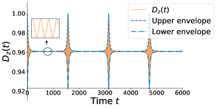
Figure 2: Time evolution and envelope of $D_{z}\left(t\right)$ in a long time scale. The envelope consists of an upper line and a lower line. The time evolution is plotted by exact numerical computation, and the envelope lines are plotted according to the analytical result in Eq. (49) with signs $+$ and $-$ respectively. The rapid oscillation with a frequency $\nu_{0}$ is shown as the sinusoidal solid line in the zoomed panel. It can be observed that the amplitude of $D_{z}\left(t\right)$ is periodic in a long time scale, showing a collapse-revival pattern and implying non-vanishing information flow between the central spin and the bath spins. Parameters: $N=1000$, $g=1$, $\omega_{s}=3$, $\omega_{b}=1$, and $T=10$.

To have an intuitive picture of this phenomenon, the trace distance $D_{z}\left(t\right)$ and its envelopes are plotted in Fig. 2. In the figure, one can observe that the amplitude of $D_{z}\left(t\right)$ decreases rapidly to almost zero first and stays for a while, then the oscillation revives and the amplitude of $D_{z}\left(t\right)$ increase to almost the original value again, and such a process will repeat. This phenomenon is essentially rooted in the superposition of oscillations with different frequencies where the phases of different oscillations will match and mismatch periodically with time.

To give a detailed analysis of the collapse-revival pattern in $D_{z}\left(t\right)$, we derive the envelopes of $D_{z}\left(t\right)$ by taking the amplitude of the rapid oscillation, and the result turns out to be

$$\Gamma_{z}(t)=\overline{D_{z}}\pm W_{z}\left(t\right),$$ (49)

where the $+$ and $-$ signs represent the upper and lower envelopes respectively.

The oscillation term $W_{z}\left(t\right)$ has a maximum value

$$\max W_{z}\left(t\right)=\frac{a_{1}}{N}\coth\frac{\omega_{b}}{2T}+\frac{a_{2}}{N^{2}}\coth^{2}\frac{\omega_{b}}{2T},$$ (50)

and thus

$$\overline{D_{z}}+\max W_{z}\left(t\right)=1,$$ (51)

implying that the trace distance $D_{z}\left(t\right)$ can almost return to its initial value, which indicates that most information can flow back to the system from the bath and there is no irreversible dissipation of the information in this scenario.

Note the effect of the number of bath spins $N$ in the collapse-revival pattern: when $N$ becomes larger, the amplitude of the collapse-revival pattern $W_{z}\left(t\right)$ will be smaller, which means the information backflow between the system and the bath will decrease, indicating a weaker non-Markovianity. This shows how the non-Markovian dynamics transits to Markovian dynamics with an increasing dimension of the bath from one aspect. As we will see below, the period of the collapse-revival pattern can also show the effect of an increasing $N$ on the transition of the Markovianity, from another aspect. We also note the different roles of the frequency detuning $\Delta=\omega_{s}-\omega_{b}$ and the bath frequency $\omega_{b}$ as well as the bath temperature $T$ in the collapse-revival pattern of the trace distance $D_{z}\left(t\right)$: $\Delta$ determines the period of collapse-revival pattern,

$$T_{cr}=\frac{2\pi}{\nu_{cr}}=\frac{\pi[2(N+1)g-\Delta]}{2g\Delta},$$ (52)

while the bath frequency $\omega_{b}$ and the temperature $T$ affect the amplitude of the collapse-revival pattern via the exponents $e^{\frac{\omega_{b}}{T}}$, $e^{\frac{2\omega_{b}}{T}}$, etc.

In addition, note that in this case, the average of the trace distance does not change with time, so the envelope is mainly determined by the oscillation amplitudes of the trace distance. This will be in sharp contrast to the behavior of the trace distance $D_{x}(t)$ in the following.

IV.2.2 Trace distance $D_{x}\left(t\right)$

For the trace distance $D_{x}\left(t\right)$, we also keep the terms up to $O(1/N^{2})$. The trace distance turns out to be

$$D_{x}^{2}\left(t\right)\doteq\overline{D_{x}^{2}}\left(t\right)+W_{x}^{2}\left(t\right)\cos\left(\nu_{0}t-\phi_{4}\right),$$ (53)

where the mean value and the amplitude of collapse-revival pattern are given as (see Appendix C for the derivation)

$$\overline{D_{x}^{2}}\left(t\right)= \frac{\left(\cosh\frac{\omega_{b}}{T}-1\right)\left(1-\frac{a_{3}}{N}\right)^{2}}{P_{-}\left(\frac{4g\Delta}{\nu_{0}}t\right)}+\frac{a_{3}^{2}P_{+}\left(\frac{4g\Delta}{\nu_{0}}t\right)}{N^{2}\left(\cosh\frac{\omega_{b}}{T}-1\right)}$$

$$+\frac{2\text{$a_{3}$}\left(\cosh\frac{\omega_{b}}{T}-1\right)\left[e^{-\frac{\omega_{b}}{T}}-\left(1-\frac{a_{3}}{N}\right)\cos\left(\frac{4g\Delta}{\nu_{0}}t\right)\right]}{NP_{-}^{2}\left(\frac{4g\Delta}{\nu_{0}}t\right)},$$ (54)

$$W_{x}^{2}\left(t\right)= 2\frac{a_{3}}{N}\left[\frac{P_{+}\left(\frac{4g\Delta}{\nu_{0}}t\right)}{P_{-}\left(\frac{4g\Delta}{\nu_{0}}t\right)}\right]^{1/2},$$ (55)

where the coefficient $a_{3}$ is

$$a_{3}=\frac{4g^{2}N^{2}}{\left(2gN-\Delta\right)^{2}}.$$ (56)

The envelope of $D_{x}(t)$ can be obtained directly,

$$\Gamma_{x}\left(t\right)=\sqrt{\overline{D_{x}^{2}}\left(t\right)\pm W_{x}^{2}\left(t\right)}.$$ (57)

Note that the mean value of $D_{x}^{2}\left(t\right)$ is dependent on the time $t$ in this case, in contrast to the case of $D_{z}(t)$.

Similar to $D_{z}\left(t\right)$, the trace distance $D_{x}\left(t\right)$ includes two oscillations, a rapid oscillation with frequency $\nu_{0}$ of $O(N)$ and a slow oscillation with frequency $\frac{4g\Delta}{\nu_{0}}$ of $O(N^{-1})$. Due to the combination of two oscillations with different frequencies, the amplitude of the rapid oscillation has a periodic collapse-revival pattern repeated with the smaller frequency $\frac{4g\Delta}{\nu_{0}}$. But in contrast to the case of $D_{z}(t)$, the average of $D_{x}(t)$ changes significantly with time while the amplitude of the rapid oscillation is only of order $N^{-1}$, so the envelope of the trace distance is mainly determined by the average in this case.

Figure 3 shows the time evolution and envelope of $D_{x}\left(t\right)$ with different $\frac{\omega_{b}}{T}$. It can be observed that the envelope consists of two lines above and below the average, and the amplitude of the trace distance exhibits a collapse-revival pattern with frequency $\frac{4g\Delta}{\nu_{0}}$, the same as $\nu_{cr}$ in $D_{z}\left(t\right)$. The two envelope lines are very close to the average of the trace distance, which verifies the results above.

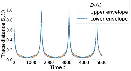
(a)

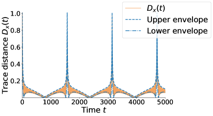
(b)

Figure 3: Time evolution and envelope of $D_{x}\left(t\right)$ in a long time scale with different bath temperatures: (a) $T=10$ and (b) $T=50$, showing a periodic collapse-revival pattern with two envelope lines. The time evolution is plotted by exact numerical computation, and the envelope lines are plotted according to the analytical result in Eq. (57) with signs $+$ and $-$ respectively. Parameters: $\omega_{s}=3,$ $N=1000$, $g=1$, and $\omega_{b}=1$.

It can be verified straightforwardly that when the number of bath spins $N$ goes to infinity asymptotically, the average of the squared trace distance $\overline{D_{x}^{2}}\left(t\right)$ will approach $1$ and the fluctuation $W_{x}^{2}\left(t\right)$ will vanish, implying the information of the system keeps almost unchanged over the evolution time and the information flow between the system and the bath is significantly suppressed in this limit, which indicates a weaker non-Markovianity of the system dynamics.

IV.2.3 Trace distances between arbitrary states of central spin

From the above results, one can see that the frequencies of the collapse-revival patterns for the trace distances $D_{x}(t)$ and $D_{z}(t)$ are the same, and Eq. (38) shows that the trace distance between two arbitrary states of the central spin can be determined by $D_{x}(t)$ and $D_{z}(t)$, so it can be immediately concluded that there exists collapse-revival structure in the trace distance between arbitrary bath spin states if it exists for the pairs of bath states $|0\rangle,|1\rangle$ or $|\pm\rangle$, given the number of the bath spins, the system-bath interaction strength and frequency detuning. It can be obtained from Eq. (38) that in general when the number of bath spins, $N$, is large, the trace distance between the central spin states evolved from two arbitrary initial states is

$$D^{2}\left(t\right)=\overline{D^{2}}\left(t\right)+W^{2}\left(t\right)\cos\left(\nu_{0}t-\phi\right),$$ (58)

where its mean value and the amplitude of oscillation are

$$\overline{D^{2}\left(t\right)}= \frac{1}{4}\alpha_{z}\overline{D_{z}}^{2}+\frac{1}{4}\alpha_{x}\overline{D_{x}^{2}}\left(t\right),$$ (59)

$$W^{2}\left(t\right)= \frac{1}{2NP_{-}\left(\nu_{cr}t\right)}\left[\alpha_{z}^{2}a_{1}^{2}\sinh^{2}\frac{\omega_{b}}{T}+\alpha_{x}^{2}a_{3}^{2}P\left(\nu_{cr}t\right)\right.$$

$$\left.-2\alpha_{x}\alpha_{z}a_{1}a_{3}\sinh\frac{\omega_{b}}{T}P^{\frac{1}{2}}\left(\nu_{cr}t\right)\cos\left(\phi_{3}-\phi_{4}\right)\right]^{1/2},$$ (60)

and the phase of the oscillation is

$$\phi=\arctan\frac{\alpha_{z}a_{1}\sinh\frac{\omega_{b}}{T}\sin\phi_{3}-\alpha_{x}a_{3}P^{\frac{1}{2}}\left(\nu_{cr}t\right)\sin\phi_{4}}{\alpha_{z}a_{1}\sinh\frac{\omega_{b}}{T}\cos\phi_{3}-\alpha_{x}a_{3}P^{\frac{1}{2}}\left(\nu_{cr}t\right)\cos\phi_{4}},$$ (61)

where $P(x)$ is defined as

$$P(x)=P_{+}(x)P_{-}(x)=\cosh^{2}\frac{\omega_{b}}{T}-\cos^{2}x.$$ (62)

The envelope of $D(t)$ can be obtained directly,

$$\Gamma_{\pm}\left(t\right)=\sqrt{\overline{D^{2}}\left(t\right)\pm W^{2}\left(t\right)}.$$ (63)

The mathematical detail of the derivation is left in Appendix D.

This suggests that the collapse-revival structure exists universally for different pairs of the central spin states, sharing the same collapse-revival frequency $\nu_{cr}$ in Eq. (48) but differing drastically in the behavior of the mean and the amplitude of the fast oscillation of the information flow.

Fig. 4 illustrates the above results for a pair of non-orthogonal system states numerically.

(a)

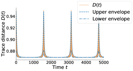
(b)

Figure 4: Time evolution and envelope of $D\left(t\right)$ with coefficients (a) $\alpha_{z}=3.614$ and $\alpha_{x}=0.188$, (b) $\alpha_{z}=3.273$ and $\alpha_{x}=0.345$. While the upper envelope always has upward peaks, the lower envelope can have upward or downward peaks: as $\alpha_{x}$ increases and $\alpha_{z}$ decreases, a downward peak of the lower envelope will move up and finally become an upward peak. Parameters: $N=1000$, $g=1$, $\omega_{s}=3$, $\omega_{b}=1$, and $T=10$.

To capture the main feature of the collapse-revival pattern, we note that for $D_{z}(t)$ the mean does not change over time and approaches $1$ and the oscillation is mainly determined by the function $P_{-}^{-1}\left(\nu_{cr}t\right)$ if only the lowest order term is considered, while for $D_{x}(t)$ the function $P_{-}^{-1}\left(\nu_{cr}t\right)$ dominates the mean value ranging from $0$ to $1$, and the amplitude of the oscillation with $O(N^{-1})$ is small compared to the mean value. So, the behavior of the general trace distance $D\left(t\right)$ can be simplified

$$\Gamma_{\pm}(t)\doteq\sqrt{\frac{\alpha_{z}}{4}\overline{D_{z}}^{2}+\frac{\alpha_{x}}{4}\frac{\cosh\frac{\omega_{b}}{T}-1}{P_{-}\left(\nu_{cr}t\right)}\pm\frac{\alpha_{z}a_{1}}{2N}\frac{\sinh\frac{\omega_{b}}{T}}{P_{-}\left(\nu_{cr}t\right)}},$$ (64)

where only the lowest order terms of $1/N$ in $D_{x}(t)$ and $D_{z}(t)$ remain, respectively, and the function $P_{-}^{-1}\left(\nu_{cr}t\right)$ determines the time evolution of the trace distance. In fact, it is exactly the function $P_{-}^{-1}(x)$ that the collapse-revival pattern stems from, as $P_{-}^{-1}(x)$ has large flat regions separated by periodic sharp peaks, plotted in Fig. 5.

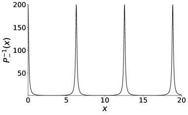
(a)

Figure 5: The behavior of the function $P_{-}^{-1}(x)$. It has large flat regions separated with periodic peaks, which determines the collapse-revival pattern. Parameters: $\omega_{b}=1$, and $T=10$.

An interesting observation of $\Gamma_{\pm}(t)$ is that while there is only one type of upper envelope $\Gamma_{+}(t)$ which has an upward peak, there are two types of lower envelopes $\Gamma_{-}(t)$ with an upward peak and a downward peak respectively. This depends on the competition between the $\alpha_{x}$ term and the $\alpha_{z}$ term in Eq. (64): if the $\alpha_{x}$ term is larger than the $\alpha_{z}$ term, the coefficient of $P_{-}^{-1}\left(\nu_{cr}t\right)$ is positive and the peak of $\Gamma_{-}(t)$ is upward, otherwise the coefficient of $P_{-}^{-1}\left(\nu_{cr}t\right)$ becomes negative and the peak of $\Gamma_{-}(t)$ turns to be downward accordingly. This is in accordance with the two types of envelopes shown in Fig. (4).

V Characteristic time scales of collapse-revival patterns

In the previous section, we obtained the behavior of information flow between the central spin and the bath, and showed the existence of the collapse-revival structure in the trace distance for arbitrary states of the central spin. To describe the collapse-revival phenomenon more quantitatively, we study typical characteristic time scales of the collapse-revival patterns in detail in this section. The time scales we consider include the period of the collapse-revival pattern, the collapse time and the revival time. We will obtain analytical results for these time scales and analyze the roles of the interaction strength, the frequency detuning, etc. in these times scales. In particular, we will consider how the number of bath qubits affects these time scales, in order to show the role of the bath dimension on the Markovianity of quantum dynamics.

V.1 Various time scales of collapse-revival pattern

The periodicity is the most prominent characteristic of the collapse-revival pattern, so we study the period of the collapse-revival pattern first.

It has been shown above that the frequency of the collapse-revival pattern is always $\nu_{cr}=\frac{4g\Delta}{\nu_{0}}$ for central spin states evolved from arbitrary initial states, so the period of the collapse-revival pattern is

$$T_{cr}=\frac{2\pi}{\nu_{cr}}=\frac{\pi(N+1)}{\Delta}-\frac{\pi}{2g}.$$ (65)

When $g$ is not small or $N$ is sufficiently large so that $gN\gg\Delta$, $T_{cr}$ can be simplified to

$$T_{cr}\doteq\frac{\pi N}{\Delta},$$ (66)

implying that the period increases with a larger $N$ or a smaller $\Delta$.

An interesting case is that if the central qubit is in resonance with the bath qubits, i.e. $\Delta=0$, or the interaction strength is zero, $g=0$, the period $T_{cr}$ goes to infinity, which indicates that the collapse-revival pattern does not exist and only the rapid oscillation appears in the information backflow. This provides the condition for the existence of the collapse-revival phenomenon when $N$ is sufficiently large,

$$g\neq 0,\;\Delta\neq 0.$$ (67)

Figure 6 shows how the number of bath qubits $N$, the coupling strength $g$ as well as the system-bath detuning $\Delta$ influence the trace distances $D_{z}(t)$ and $D_{x}(t)$, which verifies the above analytical results.

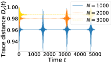
(a)

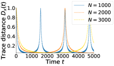
(b)

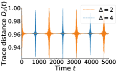
(c)

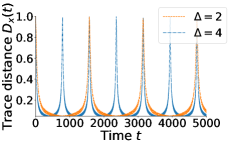
(d)

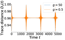
(e)

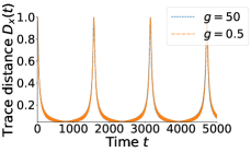
(f)

Figure 6: The behavior of the trace distances [(a), (c), (e)] $D_{z}(t)$ and [(b), (d), (f)] $D_{x}(t)$ with different values of $N$, $\Delta$, and $g$, presenting collapse-revival patterns with different periods and amplitudes. [(a), (b)] Impact of $N$ on period, where a larger $N$ gives a later revival of the information flow, leading to a weaker non-Markovianity of the central spin; [(c), (d)] influence of the frequency detuning $\Delta$ on the collapse-revival patterns with the bath frequency $\omega_{b}$ fixed. It can be seen that the period of collapse-revival patterns is inverse to $\Delta$; [(e), (f)] plot of the trace distances with different values of $g$ and that show that when $g=50$ and $g=0.5$ the two oscillations almost coincide, implying that the interaction strength $g$ has a negligible effect on the collapse-revival pattern when it is large. Parameters: [(a), (b)] $T=10$, $g=1$, $\omega_{s}=3$, and $\omega_{b}=1$; [(c), (d)] $N=1000$, $T=10$, $g=1$, and $\omega_{b}=1$; [(e), (f)] $N=1000$, $\omega_{s}=3,$ $\omega_{b}=1$, and $T=10$.

On the contrary, if $g$ is small so that $gN/\Delta=c$ has magnitude $O(1)$, the period $T_{cr}$ can be reduced to

$$T_{cr}\doteq\frac{\pi(2c-1)}{2g},$$ (68)

Figure 7 describes the collapse-revival patterns for the trace distances $D_{z}(t)$ and $D_{x}(t)$ with different values of $gN/\Delta$. In particular, when $gN/\Delta=1/2$, the period $T_{cr}=0$, so there is no collapse-revival pattern and only the rapid oscillation remains. For $gN/\Delta=1$ and $gN/\Delta=2$ with a fixed $g$, the periods of the collapse-revival patterns are proportional to $2gN/\Delta-1$, in accordance with Eq. (68).

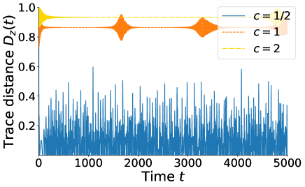
(a)

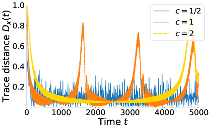
(b)

Figure 7: The behavior of the trace distances (a) $D_{z}(t)$ and (b) $D_{x}(t)$ with different $gN/\Delta$. There is no collapse-revival pattern and only rapid oscillation occurs when $gN/\Delta=1/2$, while for $gN/\Delta=1$ and $gN/\Delta=2$, the periods of collapse-revival patterns are proportional to $2gN/\Delta-1$ for the fixed $g=10^{-3}$. Parameters: $N=1000$, $\omega_{b}=1$, $T=10$, and $g=10^{-3}$.

If $g$ is sufficiently small so that $gN\ll\Delta$, Eq. (65) tells that the period is approximately

$$T_{cr}\doteq\frac{\pi}{2g},$$ (69)

implying only the interaction strength $g$ determines the period of collapse and revival in this case. This is shown in Fig. 8.

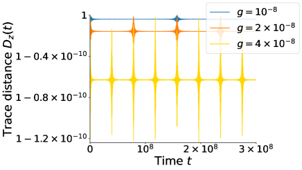
(a)

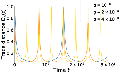
(b)

Figure 8: The behavior of the trace distances (a) $D_{z}(t)$ and (b) $D_{x}(t)$ with sufficiently small values of $g$ so that $gN\ll\Delta$. It can be seen that the period of the collapse-revival pattern becomes longer with a smaller $g$, in accordance with the analytical results. Parameters: $N=1000$, $\omega_{s}=3,$ $\omega_{b}=1$, and $T=10$.

V.2 Relation to the non-Markovianity of the central spin

In the above figures, the information backflow revives periodically in the time evolution of the central spin, so the integration over the increase in the trace distances will diverge. But one can see that a larger number of bath qubits $N$ leads to a longer collapse time and a later revival of the information backflow, so the collapse time of information backflow can characterize the non-Markovianity of the central spin dynamics in this case.

In order to characterize the non-Markovianity of the central spin dynamics by the collapse-revival structure, we define the collapse and revival times of information backflow more precisely. As the trace distance increases and decreases gradually with time, one cannot find the exact “start time” or “end time” of the collapse or revival of the information flow, so a reasonable way to define the revival time is the full width at half maximum (FWHM) of a peak in the time evolution of the trace distance, and the collapse time is the difference between the period of collapse-revival pattern and the revival time, or more intuitively the waiting time for the information backflow to revive. We provide an intuitive illustration of these definitions in Fig. 9.

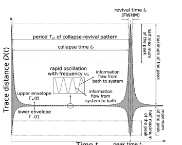
Figure 9: The conceptual sketch for the trace distance $D(t)$. The rapid oscillations of the information flow, the upper and lower envelopes, the various characteristic time scales and the information loss and backflow processes are indicated in the figure.

In detail, the maximum of the envelopes of the trace distance $D(t)$ can be obtained as

$$h_{\pm}= \max_{t}\Gamma_{\pm}(t)-\min_{t}\Gamma_{\pm}(t)$$ (70)

where

$$\max_{t}\Gamma_{\pm}(t)= \frac{1}{2}\sqrt{\alpha_{z}\overline{D_{z}}^{2}+\alpha_{x}\pm\frac{2a_{1}\alpha_{z}\coth\frac{\omega_{b}}{2T}}{N}}$$ (71)

$$\min_{t}\Gamma_{\pm}(t)= \frac{1}{2}\sqrt{\alpha_{z}\overline{D_{z}}^{2}+\alpha_{x}\tanh^{2}\frac{\omega_{b}}{2T}\pm\frac{2a_{1}\alpha_{z}\tanh\frac{\omega_{b}}{2T}}{N}}$$

and the signs $\pm$ correspond to the upper and lower envelope lines of $D(t)$, respectively. Then for a peak of $D(t)$, if $t_{p}$ is the time point that either envelope reaches its maximum, and $t_{p}-\delta,t_{p}+\delta$ are the time points that the envelope reaches the half maximum, i.e.,

$$\Gamma_{\pm}(t_{p}\pm\delta)=\frac{h_{\pm}}{2}=\frac{{\displaystyle 1}}{2}\left[\max_{t}\Gamma_{\pm}(t)+\min_{t}\Gamma_{\pm}(t)\right],$$ (72)

then the revival time can be defined as

$$t_{r}=2\delta,$$ (73)

and the collapse time as

$$t_{c}=T_{cr}-2\delta.$$ (74)

Note that the $\pm$ signs in the term $\Gamma_{\pm}(t_{p}\pm\delta)$ of Eq. (72) do not change simultaneously. The first $\pm$ sign determines which envelope line is concerned and the second $\pm$ sign denotes the two time points that the envelope reaches the half maximum.

The time points that either envelope reaches its half maximum can obtained from Eq. (63) or Eq. (64), and the result turns out to be

$$t_{p}= \frac{2k\pi}{\nu_{cr}},$$ (75)

$$\delta= \frac{\arccos\left(\cosh\frac{\omega_{b}}{T}-8\alpha_{x}\sinh^{2}\frac{\omega_{b}}{T}w^{-1}\right)}{\nu_{cr}},$$

where

$$w= \alpha_{x}\cosh\frac{\omega_{b}}{T}-\alpha_{z}\overline{D_{z}}^{2}(\cosh\frac{\omega_{b}}{T}+1)$$ (76)

$$+(\cosh\frac{\omega_{b}}{T}+1)\left(\alpha_{z}\overline{D_{z}}^{2}+\alpha_{x}\right)\sqrt{1-\frac{\alpha_{x}\text{sech}^{2}\frac{\omega_{b}}{2T}}{\alpha_{z}\overline{D_{z}}^{2}+\alpha_{x}}},$$

and $\,k=0,1,2,3,...$ denotes the $k$th revival. One can immediately have that the revival time, i.e., the full width at half maximum, is

$$t_{r}=2\delta=\frac{2\arccos\left(\cosh\frac{\omega_{b}}{T}-8\alpha_{x}\sinh^{2}\frac{\omega_{b}}{T}w^{-1}\right)}{\nu_{cr}},$$ (77)

and thus the collapse time is

$$t_{c}=T_{cr}-t_{r}=2\frac{\pi-\arccos\left(\cosh\frac{\omega_{b}}{T}-8\alpha_{x}\sinh^{2}\frac{\omega_{b}}{T}w^{-1}\right)}{\nu_{cr}}.$$ (78)

From these results, one can find that the period of the collapse-revival pattern, the revival time and the collapse time all increase with the number of bath spins $N$ as $\nu_{0}$ is linear with $N$ according to Eq. (47), but the ratio between the revival time and the collapse time keeps constant,

$$\frac{t_{c}}{t_{r}}=\frac{\pi}{\arccos\left(\cosh\frac{\omega_{b}}{T}-8\alpha_{x}\sinh^{2}\frac{\omega_{b}}{T}w^{-1}\right)}-1.$$ (79)

So, the number of bath spins mainly rescales the collapse-revival pattern of the trace distance evolution, but does not change the proportion of the collapse time and the revival time which depends on the initial state of the system and the bath temperature only. This shows the way that the dimension of the bath leads the dynamics of the central spin from non-Markovianity to Markovianity from another perspective, in addition to the influence of the bath dimension on the amplitude of the collapse-revival pattern shown in Sec. IV.2.1 and IV.2.2.

Figure 10 plots the trace distances $D_{z}(t)$ and $D_{x}(t)$ for different numbers of bath spins, $N$, and different bath temperatures $T$. The time axes for different $N$ are adjusted in proportion to $N$, so that one can compare the portion of the collapse time and revival time for different $N$.

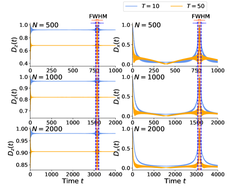
Figure 10: The full width at half maximum of a trace distance peak for $D_{z}\left(t\right)$ and $D_{x}\left(t\right)$. The time axes for different panels are adjusted in proportion to the number of bath spins, $N$, so that the portions of the collapse times and the revival times can be compared for different $N$. It shows that the period, the collapse time and the revival time of the collapse-revival structure are all proportional to $N$. The vertical dashed lines show that for a given bath temperature, the FWHM are almost the same for different number of bath spins after the adjustment of the time axis, so the ratio between the revival time and the collapse time keeps constant, which is dependent on the initial state of the central spin and the temperature of bath spins only. Parameters: $g=1$, $\omega_{s}=3$, and $\omega_{b}=1$.

Remark. While the periodic patterns of the information backflow change for different states of the central spin, they share crucial similarities. The most important one is that the information flow collapses and reappears when the bath dimension is finite, and the revival amplitude does not reduce over time, implying the information backflow can occur periodically for an arbitrary evolution time. As the revival of the information backflow indicates a violation of the CPTP divisibility, the more frequent revivals of the information backflow imply a stronger non-Markovianity of the system dynamics. Therefore, the period and the collapse time of the collapse-revival pattern may serve as a characterization of the non-Markovianity in this case, while the integration over the information backflow may diverge. As is shown in this section, both the period and the collapse time of the collapse-revival pattern are proportional to the number of bath spins when the number of bath spins is sufficiently large, so a larger bath dimension leads to later revivals of information backflow. When the number of the bath spins goes to infinity, the period and the collapse time will become infinitely long, so the revival of the information backflow will actually never occur in this limit. This tells the role of the bath dimension in the Markovianity of quantum dynamics and shows how the transition of quantum dynamics from non-Markovian to Markovian occurs when the bath grows from finite dimension to infinite dimension.

VI Conclusion and outlook

In this work we consider a simple but nontrivial isotropic central spin model to analyze the influence of bath dimension on the non-Markovianity of the system dynamics. We obtain the dynamics of the central spin with the bath spins in a symmetric thermal equilibrium state initially, and compute the trace distance for different pairs of initial states of the central spin to study the non-Markovianity of the system dynamics.

We mainly work in the regime where the number of bath spins, $N$, is sufficiently large compared to $T/\omega_{b}$ but still finite. In this case, approximate results are obtained for the trace distances between arbitrary system states. The results show that oscillations with dramatically different frequencies appear in the trace distances, which leads to the collapse and revival phenomenon in the time evolution of the trace distances. We obtain the conditions for the existence of the collapse-revival phenomenon, analyze the roles of different physical parameters such as the interaction strength, the system-bath detuning, etc. in the trace distances in detail, and derive typical characteristic time scales of the trace distance, including the period, the collapse time, and the revival time of the information backflow. These results show how the collapse-revival pattern changes with an increasing number of bath qubits, and reveal the effect of bath dimension in the transition of non-Markovian quantum dynamics to Markovian quantum dynamics.

The results show that the collapse and revival of information backflow does not recede with time and occurs periodically in the current model. A larger number of bath spins or weaker system-bath interaction will give a later and less frequent revival of the information backflow, and the information backflow will finally vanish when the number of bath spins goes to infinity or the system-bath interaction goes to zero. This shows how the transition of the Markovianity of the central spin dynamics occurs in the limit of large number of bath spins.

We hope this work can provide a new perspective on the non-Markovianity of quantum dynamics, particularly in the presence of a large but finite-dimensional environment, and a useful approach to the characterization of non-Markovianity for this case.

Appendix A EVOLUTION OF THE SYSTEM

A.1 Eigenvalues and eigenstates of total Hamiltonian

A symmetric thermal state can be represented by a superposition of Dicke states, which inspires us to consider the evolution of a system-bath joint state $\lvert\psi_{sb}^{(M)}\left(0\right)\rangle=\left(\zeta_{0}\lvert 0\rangle+\zeta_{1}\lvert 1\rangle\right)\otimes\lvert J,M\rangle$ under the total Hamiltonian

$$H_{tot}=\frac{\omega_{s}}{2}\sigma_{z}^{(s)}+\omega_{b}S_{z}+2g\left(\sigma_{+}^{(s)}S_{-}+\sigma_{-}^{(s)}S_{+}+\sigma_{z}^{(s)}S_{z}\right).$$ (80)

The initial joint state of the system and bath can be written as

$$\rho_{sb}\left(0\right)=\sum_{M=-J}^{J}\frac{e^{-\frac{M\omega_{b}}{T}}}{Q}\lvert\psi_{sb}^{(M)}\left(0\right)\rangle\langle\psi_{sb}^{(M)}\left(0\right)\rvert,\,\,Q=\frac{e^{\frac{(J+1)\omega_{b}}{T}}-e^{-\frac{J\omega_{b}}{T}}}{e^{\frac{\omega_{b}}{T}}-1}.$$ (81)

After the time evolution $U\left(t\right)=e^{-iH_{tot}t}$, the joint state evolves into

$$\rho_{sb}\left(t\right)=U\left(t\right)\rho_{sb}\left(0\right)U\left(t\right)^{\dagger}=\sum_{M=-J}^{J}\frac{e^{-\frac{M\omega_{b}}{T}}}{Q}\lvert\psi_{sb}^{(M)}\left(t\right)\rangle\langle\psi_{sb}^{(M)}\left(t\right)\rvert,$$ (82)

where $\lvert\psi_{sb}^{(M)}\left(t\right)\rangle=e^{-iH_{tot}t}\lvert\psi_{sb}^{(M)}\left(0\right)\rangle$.

Note that the subspaces spanned by the pairs of states $\left\{\lvert 0\rangle\otimes\lvert J,M\rangle,\lvert 1\rangle\otimes\lvert J,M-1\rangle\right\}$, $-J+1\leq M\leq J$, are invariant under the total Hamiltonian. One can find the reduced Hamiltonian in the each subspace to be

$$H_{M}=\left[\begin{array}[]{cc}\frac{\omega_{s}}{2}-M\left(\omega_{b}+2g\right)&2g\sqrt{\left(J-M+1\right)\left(J+M\right)}\\ 2g\sqrt{\left(J-M+1\right)\left(J+M\right)}&-\frac{\omega_{s}}{2}-(M-1)\left(\omega_{b}-2g\right)\end{array}\right].$$ (83)

Then the eigenvalues of $H_{M}$ can be obtained as

$$\lambda_{M,\pm}=E_{M}\pm F_{M},$$ (84)

where $E_{M}$ and $F_{M}$ are functions dependent on $M$,

$$E_{M}=-g+\frac{2M-1}{2}\omega_{b},\,\,F_{M}=\sqrt{G_{M}^{2}+4\left(J-M+1\right)\left(J+M\right)g^{2}}.$$ (85)

Here $G_{M}=\left(2M-1\right)g+\frac{\Delta}{2},$and $\Delta=\omega_{s}-\omega_{b}$ is the frequency detuning. The eigenstates of $H_{M}$ can also be obtained,

$$\lvert\Phi\rangle_{M,\pm}=c_{M,\pm}\lvert 0\rangle\lvert J,M\rangle+d_{M,\pm}\lvert 1\rangle\lvert J,M-1\rangle,$$ (86)

corresponding to the eigenvalues $\lambda_{M,\pm}$ respectively, where

$$c_{M,\pm}=\pm{\rm sgn}(g)\sqrt{\frac{1}{2}\left(1\mp\frac{G_{M}}{F_{M}}\right)},\;d_{M,\pm}=\sqrt{\frac{1}{2}\left(1\pm\frac{G_{M}}{F_{M}}\right)}.$$ (87)

According to Eq. (86), one can write the states $\lvert 0\rangle\otimes\lvert J,M\rangle$ and $\lvert 1\rangle\otimes\lvert J,M-1\rangle$ as a superposition of the eigenstates $\lvert\Phi\rangle_{M,\pm}$,

$$\lvert 0\rangle\lvert J,M\rangle= \frac{d_{M,-}}{K_{M}}\lvert\Phi\rangle_{M,+}-\frac{d_{M,+}}{K_{M}}\lvert\Phi\rangle_{M,-},$$ (88)

$$\lvert 1\rangle\lvert J,M-1\rangle= -\frac{c_{M,-}}{K_{M}}\lvert\Phi\rangle_{M,+}+\frac{c_{M,+}}{K_{M}}\lvert\Phi\rangle_{M,-},$$

where $K_{M}=c_{M,+}d_{M,-}-c_{M,-}d_{M,+}$ and it can be verified that $K_{M}={\rm sgn}(g)$.

Two additional eigenstates, $\lvert\Phi\rangle_{-J}=\lvert 0\rangle\otimes\lvert J,-J\rangle$ and $\lvert\Phi\rangle_{J+1}=\lvert 1\rangle\otimes\lvert J,J\rangle$ are also contained in the above invariant subspaces with $M=-J$ and $M=J+1$ respectively, and corresponding eigenvalues are

$$\lambda_{-J}=E_{M}-{\rm sgn}(G_{M})G_{M},\;\lambda_{J+1}=E_{M}+{\rm sgn}(G_{M})G_{M}.$$ (89)

Note that there is one non-physical eigenstate in each of those two invariant subspaces, $\lvert 1\rangle\otimes\lvert J,-J-1\rangle$ for $M=-J$ and $\lvert 0\rangle\otimes\lvert J,M\rangle$ for $M=J+1$. However, these two non-physical eigenstates will not affect the validity of Eq. (88) with $M=-J,J+1$, since they vanish in Eq. (88) when $M$ takes $-J$ or $J+1$,

$$\lvert 0\rangle\otimes\lvert J,-J\rangle= (d_{J,-}c_{J,+}-d_{J,+}c_{J,-})\lvert 0\rangle\otimes\lvert J,-J\rangle/K_{J}=\lvert 0\rangle\otimes\lvert J,-J\rangle,$$ (90)

$$\lvert 1\rangle\otimes\lvert J,J\rangle= (-c_{J+1,-}d_{J+1,+}+c_{J+1,+}d_{J+1,-})\lvert 1\rangle\otimes\lvert J,J\rangle/K_{J+1}=\lvert 1\rangle\otimes\lvert J,J\rangle.$$

So the general eigenstate expression (86) can also work for the two additional eigenstates.

A.2 Joint evolution of the system and bath

The eigenvalues and the eigenstates of $H_{tot}$ lead to the derivation of the exact reduced dynamics of the central spin. The evolved state can be decomposed into the eigenstates of $H_{tot}$,

$$\lvert\psi_{sb}^{(M)}\left(0\right)\rangle=e^{-iH_{tot}t}\left(\zeta_{0}\lvert 0\rangle+\zeta_{1}\lvert 1\rangle\right)\lvert J,M\rangle=\sum_{M^{\prime}=-J}^{J+1}\sum_{\pm}D_{M^{\prime},\pm}e^{-i\lambda_{M^{\prime},\pm}t}\lvert\Phi\rangle_{M^{\prime},\pm},$$ (91)

where

$$D_{M^{\prime},\pm}=\left(\pm\zeta_{0}d_{M^{\prime},\mp}\delta_{M,M^{\prime}}\mp\zeta_{1}c_{M^{\prime},\mp}\delta_{M,M^{\prime}-1}\right)/K_{M}.$$ (92)

The reduced evolution of the central spin can be obtained as

$$\rho_{s}\left(t\right)=\mathrm{Tr}_{b}\rho_{sb}\left(t\right)=\sum_{M,M^{\prime\prime}=-J}^{J}\frac{e^{-\frac{M\omega_{b}}{T}}}{Q}\langle J,M^{\prime\prime}\lvert\psi_{SM}\left(t\right)\rangle\langle\psi_{SM}\left(t\right)\rvert J,M^{\prime\prime}\rangle.$$ (93)

To facilitate the computation, $\rho_{s}\left(t\right)$ can be written in the matrix form

$$\rho_{s}\left(t\right)=\left[\begin{array}[]{cc}\rho_{00}(t)&\rho_{01}(t)\\ \rho_{10}(t)&\rho_{11}(t)\end{array}\right],$$ (94)

where

$$\rho_{00}(t)= \sum_{M,M^{\prime\prime}=-J}^{J}\frac{e^{-\frac{M\omega_{b}}{T}}}{Q}\left(\sum_{\pm}D_{M^{\prime\prime},\pm}e^{-i\lambda_{M^{\prime\prime},\pm}t}c_{M^{\prime\prime},\pm}\right)\left(\sum_{\pm}D_{M^{\prime\prime},\pm}^{*}e^{i\lambda_{M^{\prime\prime},\pm}t}c_{M^{\prime\prime},\pm}\right)$$ (95)

$$= \left|\zeta_{0}\right|^{2}-\left(\left|\zeta_{0}\right|^{2}-e^{\frac{\omega_{b}}{T}}\left|\zeta_{1}\right|^{2}\right)\sum_{M=-J}^{J}\frac{e^{-\frac{M\omega_{b}}{T}}}{Q}\frac{1}{2}\left(1-\frac{G_{M}^{2}}{F_{M}^{2}}\right)\left[1-\cos\left(2F_{M}t\right)\right],$$

$$\rho_{11}(t)= \sum_{M,M^{\prime\prime}=-J}^{J}\frac{e^{-\frac{M\omega_{b}}{T}}}{Q}\left(\sum_{\pm}D_{M^{\prime\prime}+1,\pm}e^{-i\lambda_{M^{\prime\prime}+1,\pm}t}d_{M^{\prime\prime}+1,\pm}\right)\left(\sum_{\pm}D_{M^{\prime\prime}+1,\pm}^{*}e^{i\lambda_{M^{\prime\prime}+1,\pm}t}d_{M^{\prime\prime}+1,\pm}\right)$$ (96)

$$= \left|\zeta_{1}\right|^{2}+\left(\left|\zeta_{0}\right|^{2}-e^{\frac{\omega_{b}}{T}}\left|\zeta_{1}\right|^{2}\right)\sum_{M=-J}^{J}\frac{e^{-\frac{M\omega_{b}}{T}}}{Q}\frac{1}{2}\left(1-\frac{G_{M}^{2}}{F_{M}^{2}}\right)\left[1-\cos\left(2F_{M}t\right)\right],$$

$$\rho_{01}(t)= \sum_{M,M^{\prime\prime}=-J}^{J}\frac{e^{-\frac{M\omega_{b}}{T}}}{Q}\left(\sum_{\pm}D_{M^{\prime\prime},\pm}e^{-i\lambda_{M^{\prime\prime},\pm}t}c_{M^{\prime\prime},\pm}\right)\left(\sum_{\pm}D_{M^{\prime\prime}+1,\pm}^{*}e^{i\lambda_{M^{\prime\prime}+1,\pm}t}d_{M^{\prime\prime}+1,\pm}\right)$$ (97)

$$= \zeta_{0}\zeta_{1}^{*}\sum_{M=-J}^{J}\frac{e^{-\frac{M\omega_{b}}{T}}}{Q}\left[\cos\left(\omega_{b}t\right)+i\sin\left(\omega_{b}t\right)\right]\left[\cos\left(F_{M}t\right)+i\frac{G_{M}}{F_{M}}\sin\left(F_{M}t\right)\right]\left[\cos\left(F_{M+1}t\right)+i\frac{G_{M+1}}{F_{M+1}}\sin\left(F_{M+1}t\right)\right],$$

$$\rho_{10}(t)= \rho_{01}^{*}(t)$$ (98)

$$= \zeta_{0}^{*}\zeta_{1}\sum_{M=-J}^{J}\frac{e^{-\frac{M\omega_{b}}{T}}}{Q}\left[\cos\left(\omega_{b}t\right)-i\sin\left(\omega_{b}t\right)\right]\left[\cos\left(F_{M}t\right)-i\frac{G_{M}}{F_{M}}\sin\left(F_{M}t\right)\right]\left[\cos\left(F_{M+1}t\right)-i\frac{G_{M+1}}{F_{M+1}}\sin\left(F_{M+1}t\right)\right].$$

If we represent the final density matrix of the central spin by a Bloch vector $\boldsymbol{v}(t)=[x(t),y(t),z(t)]$, then $\boldsymbol{v}(t)$ can be worked out as

$$x(t)= \rho_{01}(t)+\rho_{10}(t)$$

$$= \left(\zeta_{0}\zeta_{1}^{*}+\zeta_{0}^{*}\zeta_{1}\right)X_{1}\left(t\right)+i\left(\zeta_{0}\zeta_{1}^{*}-\zeta_{0}^{*}\zeta_{1}\right)X_{2}\left(t\right)$$

$$= x_{0}X_{1}\left(t\right)+y_{0}X_{2}\left(t\right),$$

$$y(t)= i\left(\rho_{01}(t)-\rho_{10}(t)\right)$$

$$= i\left(\zeta_{0}\zeta_{1}^{*}-\zeta_{0}^{*}\zeta_{1}\right)X_{1}\left(t\right)-\left(\zeta_{0}\zeta_{1}^{*}+\zeta_{0}^{*}\zeta_{1}\right)X_{2}\left(t\right)$$ (99)

$$= y_{0}X_{1}\left(t\right)-x_{0}X_{2}\left(t\right),$$

$$z(t)= \rho_{00}(t)-\rho_{11}(t)$$

$$= z_{0}-z_{0}\left(1+e^{\frac{\omega_{b}}{T}}\right)Z(t)-\left(1-e^{\frac{\omega_{b}}{T}}\right)Z(t)$$

$$= z_{0}Z_{1}\left(t\right)+Z_{2}\left(t\right),$$

where $X_{1}\left(t\right)$, $X_{2}\left(t\right)$ , $Z_{1}\left(t\right)$ and $Z_{2}\left(t\right)$ are

$$X_{1}\left(t\right)= \sum_{M=-J}^{J}\frac{e^{-\frac{M\omega_{b}}{T}}}{Q}\left[\sin\left(\omega_{b}t\right)A_{M}\left(t\right)+\cos\left(\omega_{b}t\right)B_{M}\left(t\right)\right],$$ (100)

$$X_{2}\left(t\right)= \sum_{M=-J}^{J}\frac{e^{-\frac{M\omega_{b}}{T}}}{Q}\left[\cos\left(\omega_{b}t\right)A_{M}\left(t\right)-\sin\left(\omega_{b}t\right)B_{M}\left(t\right)\right],$$ (101)

$$Z_{1}\left(t\right)= 1-\left(1+e^{\frac{\omega_{b}}{T}}\right)\sum_{M=-J}^{J}\frac{e^{-\frac{M\omega_{b}}{T}}}{Q}C_{M}\left(t\right),$$ (102)

$$Z_{2}\left(t\right)= \left(e^{\frac{\omega_{b}}{T}}-1\right)\sum_{M=-J}^{J}\frac{e^{-\frac{M\omega_{b}}{T}}}{Q}C_{M}\left(t\right).$$ (103)

In the above equations, $A_{M}\left(t\right)$, $B_{M}\left(t\right)$ and $C_{M}\left(t\right)$ are defined as

$$A_{M}\left(t\right)= -\frac{G_{M+1}}{F_{M+1}}\cos\left(F_{M}t\right)\sin\left(F_{M+1}t\right)-\frac{G_{M}}{F_{M}}\sin\left(F_{M}t\right)\cos\left(F_{M+1}t\right),$$

$$B_{M}\left(t\right)= \cos\left(F_{M}t\right)\cos\left(F_{M+1}t\right)-\frac{G_{M}}{F_{M}}\frac{G_{M+1}}{F_{M+1}}\sin\left(F_{M}t\right)\sin\left(F_{M+1}t\right),$$ (104)

$$C_{M}\left(t\right)= \frac{1}{2}\left(1-\frac{G_{M}^{2}}{F_{M}^{2}}\right)\left[1-\cos\left(2F_{M}t\right)\right].$$

Appendix B the derivation of $Z_{1}\left(t\right)$

The approximation of $Z_{1}\left(t\right)$ can be obtained by replacing $M$ with $\xi=(M+J)/N$. We keep the terms up to $O(1/N^{2})$, and it turns out to be

$$Z_{1}\left(t\right)= 1-\left(1+e^{\frac{\omega_{b}}{T}}\right)\sum_{M=-J}^{J}\frac{e^{-\frac{M\omega_{b}}{T}}}{Q}\frac{1}{2}\left(1-\frac{G_{M}^{2}}{F_{M}^{2}}\right)\left[1-\cos\left(2F_{M}t\right)\right]$$ (105)

$$= 1-\left(1+e^{\frac{\omega_{b}}{T}}\right)\frac{e^{\frac{N\omega_{b}}{2T}}}{Q}\sum_{\xi}e^{-\frac{\xi N\omega_{b}}{T}}\sum_{j}\left(a_{j}\xi^{j}\right)\left[1-\cos\left(\sum_{k}\nu_{k}\xi^{k}t\right)\right]$$

$$\simeq 1-\left(1+e^{\frac{\omega_{b}}{T}}\right)\frac{e^{\frac{N\omega_{b}}{2T}}}{Q}\sum_{\xi}e^{-\frac{\xi N\omega_{b}}{T}}\left(a_{0}+a_{1}\xi+a_{2}\xi^{2}\right)\left[1-\cos\left(\nu_{0}t+\nu_{1}\xi t\right)\right],$$

where $a_{0}=0$, $a_{1}={\displaystyle\frac{8g^{2}N(N+1)}{\left[2(N+1)g-\Delta\right]^{2}}}$, $a_{2}={\displaystyle-\frac{8g^{2}N^{2}\left[2(N+1)g+\Delta\right]^{2}}{\left[2(N+1)g-\Delta\right]^{4}}}$, $\nu_{0}=\left|2(N+1)g-\Delta\right|$ and $\nu_{1}=\frac{4Ng\Delta}{\nu_{0}}$. Here the power series for the amplitude and the phase are valid for $g{\displaystyle<\frac{\left(3N+1\right)\Delta-2\sqrt{\Delta^{2}N(2N+1)}}{2(N+1)^{2}}}$ and ${\displaystyle g>\frac{\left(3N+1\right)\Delta+2\sqrt{\Delta^{2}N(2N+1)}}{2(N+1)^{2}}}$ to guarantee the convergence of the Taylor series. The summation of $\xi$ runs from $0$ to $1$ with a step size $1/N$ and can be obtained analytically,

$$\sum_{\xi}e^{\frac{-\xi N\omega_{b}}{T}}\left[1-\cos\left(\nu_{0}t+\nu_{1}\xi t\right)\right]\simeq e^{\frac{\omega_{b}}{2T}}\left[\frac{1}{\sqrt{2P_{-}\left(\frac{\nu_{1}t}{N}\right)}}\cos\left(\nu_{0}t-\phi_{0}\right)+\frac{\text{csch}\frac{\omega_{b}}{2T}}{2}\right],$$ (106)

$$\sum_{\xi}e^{\frac{-\xi N\omega_{b}}{T}}\xi\left[1-\cos\left(\nu_{0}t+\nu_{1}\xi t\right)\right]\simeq \frac{1}{2NP_{-}\left(\frac{\nu_{1}t}{N}\right)}\cos\left(\nu_{0}t-\phi_{1}\right)+\frac{\text{csch}^{2}\frac{\omega_{b}}{2T}}{4N},$$

$$\sum_{\xi}e^{\frac{-\xi N\omega_{b}}{T}}\xi^{2}\left[1-\cos\left(\nu_{0}t+\nu_{1}\xi t\right)\right]\simeq \frac{1}{2N^{2}}\sqrt{\frac{P_{+}\left(\frac{\nu_{1}t}{N}\right)}{P_{-}^{3}\left(\frac{\nu_{1}t}{N}\right)}}\cos\left(\nu_{0}t-\phi_{2}\right)+\frac{\sinh\frac{\omega_{b}}{T}\text{csch}^{4}\frac{\omega_{b}}{2T}}{8N^{2}},$$

where the function

$$P_{\pm}\left(x\right)=\cosh\frac{\omega_{b}}{T}\pm\cos x$$ (107)

will be critical to the characteristic time scales of the collapse-revival pattern, and the sign $\simeq$ denotes that only the terms $e^{\frac{\omega_{b}}{T}O(N)}$ remain and the terms $e^{\frac{\omega_{b}}{T}O(1)}$ are neglected since $N$ is large. The phases $\phi_{0},\phi_{1},$and $\phi_{2}$ are

$$\phi_{0} =\arctan\frac{\sin\frac{\text{$\nu_{1}$}t}{N}}{\cos\frac{\text{$\nu_{1}$}t}{N}-e^{\frac{\omega_{b}}{T}}},$$

$$\phi_{1} =\arctan\frac{\sinh\frac{\omega_{b}}{T}\sin\frac{\text{$\nu_{1}$}t}{N}}{1-\cosh\frac{\omega_{b}}{T}\cos\frac{\text{$\nu_{1}$}t}{N}},$$ (108)

$$\phi_{2} =-\arctan\frac{\left(\cosh\frac{2\omega_{b}}{T}-3\right)\sin\frac{\text{$\nu_{1}$}t}{N}+\cosh\frac{\omega_{b}}{T}\sin\frac{2\text{$\nu_{1}$}t}{N}}{\sinh\frac{\omega_{b}}{T}\left(\cos\frac{2\text{$\nu_{1}$}t}{N}-3\right)+\sinh\frac{2\omega_{b}}{T}\cos\frac{\text{$\nu_{1}$}t}{N}}.$$

It can be seen from Eq. (106) that

$$\sum_{\xi}e^{\frac{-\xi N\omega_{b}}{T}}\xi^{k}\left[1-\cos\left(\nu_{0}t+\nu_{1}\xi t\right)\right]\sim 1/N^{k},$$ (109)

and we approximate the amplitude term up to $O(1/N^{2})$ in Eq. (105). Then the approximation of $Z_{1}\left(t\right)$ can be obtained as

$$Z_{1}\left(t\right)\simeq 1-\left(1+e^{\frac{\omega_{b}}{T}}\right)\frac{e^{\frac{N\omega_{b}}{2T}}}{Q}\sum_{\xi}e^{\frac{-\xi N\omega_{b}}{T}}\left(a_{0}+a_{1}\xi+a_{2}\xi^{2}\right)\left[1-\cos\left(\nu_{0}t+\nu_{1}\xi t\right)\right]$$ (110)

$$\simeq 1+a_{1}\coth\frac{\omega_{b}}{2T}-a_{2}\coth^{2}\frac{\omega_{b}}{2T}-\frac{\sinh\frac{\omega_{b}}{T}}{NP_{-}\left(\frac{\nu_{1}t}{N}\right)}$$

$$\times\sqrt{a_{1}^{2}+\frac{a_{2}^{2}}{N^{2}}\frac{P_{+}\left(\frac{\nu_{1}t}{N}\right)}{P_{-}\left(\frac{\nu_{1}t}{N}\right)}+\frac{2a_{1}a_{2}}{N}\sqrt{\frac{P_{+}\left(\frac{\nu_{1}t}{N}\right)}{P_{-}\left(\frac{\nu_{1}t}{N}\right)}}\cos\left(\phi_{1}-\phi_{2}\right)}\cos\left(\nu_{0}t-\phi_{3}\right),$$

where

$$\phi_{3}=\arctan\frac{a_{1}N\sqrt{P_{-}\left(\frac{\nu_{1}t}{N}\right)}\sin\phi_{1}+a_{2}\sqrt{P_{+}\left(\frac{\nu_{1}t}{N}\right)}\sin\phi_{2}}{a_{1}N\sqrt{P_{-}\left(\frac{\nu_{1}t}{N}\right)}\cos\phi_{1}+a_{2}\sqrt{P_{+}\left(\frac{\nu_{1}t}{N}\right)}\cos\phi_{2}}.$$ (111)

The last $\simeq$ in Eq. (110) comes from the approximation ${\displaystyle\frac{e^{\left(1+\frac{N}{2}\right)\frac{\omega_{b}}{T}}}{Q}=\frac{e^{\frac{(N+1)\omega_{b}}{T}}}{e^{\frac{(N+1)\omega_{b}}{T}}-1}\simeq 1}$ since $N$ is sufficiently large.

Appendix C the approximation of $D_{x}^{2}\left(t\right)$

We start with the density matrix $\rho_{s}\left(t\right)$ for the initial states $|\pm\rangle$,

$$\rho_{s}(t)=\begin{bmatrix}\rho_{00}(t)&\pm\rho_{01}(t)\\ \pm\rho_{01}^{*}(t)&\rho_{11}(t)\end{bmatrix},$$ (112)

and the trace distance between two initial states $|\pm\rangle$ is

$$D_{x}^{2}\left(t\right)=|\rho_{01}(t)|^{2}.$$ (113)

According to Eqs. (99)-(101), the matrix element $\rho_{01}(t)$ can be obtained up to $O(1/N^{2})$ as

$$\rho_{01}(t)= \frac{e^{-i\omega_{b}t}}{2}\sum_{M=-J}^{J}\frac{e^{-\frac{M\omega_{b}}{T}}}{Q}\sum_{k,l=0}^{1}\left[\frac{1}{2}+(-1)^{k}\frac{G_{M}}{2F_{M}}\right]\left[\frac{1}{2}+(-1)^{l}\frac{G_{M+1}}{2F_{M+1}}\right]e^{i\left[(-1)^{k}F_{M}+(-1)^{l}F_{M+1}\right]t}$$ (114)

$$\approx \frac{e^{\frac{N\omega_{b}}{2T}}e^{-i\omega_{b}t}}{2Q}\sum_{\xi}e^{-\frac{\xi N\omega_{b}}{T}}\sum_{h=1}^{4}(\mu_{h,0}+\mu_{h,1}\xi+\mu_{h,2}\xi^{2})e^{-i(\nu_{h,0}+\nu_{h,1}\xi)t}.$$

The Taylor expansion is valid in the regions ${\displaystyle g<\frac{\left(3N+1\right)\Delta-2\sqrt{\Delta^{2}N(2N+1)}}{2(N+1)^{2}}}$ and ${\displaystyle g>\frac{\left(3N+1\right)\Delta+2\sqrt{\Delta^{2}N(2N+1)}}{2(N+1)^{2}}}$, the same as that in $D_{z}\left(t\right)$. The coefficients in the summation are listed in Table 1.

					$2gN-\Delta>0$				$2gN-\Delta<0$
		$\nu_{h,0}$	$\nu_{h,1}$		$\mu_{h,0}$	$\mu_{h,1}$	$\mu_{h,2}$		$\mu_{h,0}$	$\mu_{h,1}$	$\mu_{h,2}$
$h=1$		$\frac{\nu_{1}}{2N}$	$0$		$0$	$a_{3}$	$-a_{3}$		$\frac{a_{3}}{N}$	$a_{3}$	$-a_{3}$
$h=2$		$-\frac{\nu_{1}}{2N}$	$0$		$\frac{a_{3}}{N}$	$a_{3}$	$-a_{3}$		$0$	$a_{3}$	$-a_{3}$
$h=3$		$\nu_{0}$	$\nu_{1}$		$1-\frac{a_{3}}{N}$	$-2a_{3}$	$a_{3}$		$0$	$0$	$a_{3}$
$h=4$		$-\nu_{0}$	$-\nu_{1}$		$0$	$0$	$a_{3}$		$1-\frac{a_{3}}{N}$	$-2a_{3}$	$a_{3}$

Table 1: The coefficients for the first few terms up to $O\left(1/N^{2}\right)$ in the amplitude and phase series of $\rho_{01}(t)$. Here $\nu_{0}$ and $\nu_{1}$ are the parameters of $D_{z}\left(t\right)$, and $a_{3}=\frac{4g^{2}N^{2}}{\left(2gN-\Delta\right)^{2}}$. It turns out that the coefficients are different for $2gN-\Delta>0$ and $2gN-\Delta<0$.

The summation in $\rho_{01}(t)$ can be worked out as

$$\sum_{\xi}e^{-\frac{\xi N\omega_{b}}{T}}e^{-i\left(\nu_{0}+\nu_{1}\xi\right)t} \simeq\frac{e^{-i\nu_{0}t}}{1-e^{-\frac{\omega_{b}}{T}-\frac{i\nu_{1}t}{N}}},$$ (115)

$$\sum_{\xi}\xi e^{-\frac{\xi N\omega_{b}}{T}}e^{-i\left(\nu_{0}+\nu_{1}\xi\right)t} \simeq\frac{e^{\frac{\omega_{b}}{T}-\frac{it(\nu_{0}N+\nu_{1})}{N}}}{N\left(e^{\frac{\omega_{b}}{T}}-e^{-\frac{i\nu_{1}t}{N}}\right)^{2}},$$

$$\sum_{\xi}\xi^{2}e^{-\frac{\xi N\omega_{b}}{T}}e^{-i\left(\nu_{0}+\nu_{1}\xi\right)t} \simeq\frac{\left(e^{\frac{\omega_{b}}{T}}+e^{-\frac{i\nu_{1}t}{N}}\right)\exp\left(-\frac{it(\nu_{0}N+\nu_{1})}{N}+\frac{(N+1)\omega_{b}}{T}-\frac{N\omega_{b}}{T}\right)}{N^{2}\left(e^{\frac{\omega_{b}}{T}}-e^{-\frac{i\nu_{1}t}{N}}\right)^{3}}.$$

It can be seen that the matrix elements $\rho_{01}(t)$ are conjugate for $2gN-\Delta>0$ and $2gN-\Delta<0$, implying that the $D_{x}^{2}\left(t\right)$ for the two cases are the same. Then trace distance between $|+\rangle,|-\rangle$ can be obtained up to $O(1/N^{2})$ as

$$D_{x}^{2}\left(t\right)\simeq 2\frac{a_{3}}{N}\sqrt{\frac{P_{+}\left(\frac{\nu_{1}t}{N}\right)}{P_{-}\left(\frac{\nu_{1}t}{N}\right)}}\cos\left(\nu_{0}t+\phi_{4}\right)+\frac{a_{3}^{2}P_{+}\left(\frac{\nu_{1}t}{N}\right)}{N^{2}\left(\cosh\frac{\omega_{b}}{T}-1\right)}$$ (116)

$$+\frac{\left(\cosh\frac{\omega_{b}}{T}-1\right)\left(1-\frac{a_{3}}{N}\right)^{2}}{P_{-}\left(\frac{\nu_{1}t}{N}\right)}+\frac{2\text{$a_{3}$}\left(\cosh\frac{\omega_{b}}{T}-1\right)\left[e^{-\frac{\omega_{b}}{T}}-\left(1-\frac{a_{3}}{N}\right)\cos\left(\frac{\nu_{1}}{N}t\right)\right]}{NP_{-}^{2}\left(\frac{\nu_{1}t}{N}\right)},$$

where the phase $\phi_{4}$ is

$$\phi_{4}=\arctan\left\{\frac{\left(e^{-\frac{\omega_{b}}{T}}\cos\frac{\nu_{1}t}{N}+\cosh\frac{\omega_{b}}{T}\right)\left[\left(N-a_{3}\right)P_{-}\frac{\nu_{1}t}{N}+\text{{\hbox{a_{3}e^{-\frac{\omega_{b}}{T}}}}}\right]-\text{{\hbox{a_{3}}}}\left(e^{\frac{\omega_{b}}{T}}\cos\frac{\nu_{1}t}{N}+\cosh\frac{\omega_{b}}{T}\right)}{\left(e^{-\frac{\omega_{b}}{T}}\cos\frac{\nu_{1}t}{N}-\cosh\frac{\omega_{b}}{T}\right)\left[\left(N-a_{3}\right)P_{-}\frac{\nu_{1}t}{N}+\text{{\hbox{a_{3}}}}e^{-\frac{\omega_{b}}{T}}\right]+\text{{\hbox{a_{3}}}}\left(e^{\frac{\omega_{b}}{T}}\cos\frac{\nu_{1}t}{N}-\cosh\frac{\omega_{b}}{T}\right)}\tan\frac{\nu_{1}t}{2N}\right\}.$$ (117)

Appendix D Trace distance for arbitrary central spin states

The trace distance between two states of the central spin at time $t$ given arbitrary initial states $\rho_{1}(0),\,\rho_{2}(0)$ can be obtained as

$$D\left(t\right)=\frac{1}{2}\sqrt{\alpha_{z}D_{z}^{2}(t)+\alpha_{x}D_{x}^{2}(t)},$$ (118)

where the coefficients $\alpha_{x}=[x_{1}(0)-x_{2}(0)]^{2}+[y_{1}(0)-y_{2}(0)]^{2}$ and $\alpha_{z}=[z_{1}(0)-z_{2}(0)]^{2}$ are determined by the two initial states, and the functions $D_{z}^{2}(t)$ and $D_{x}^{2}(t)$ represent the trace distance given the initial states $|0\rangle,|1\rangle$ and given the initial states $|\pm\rangle$ respectively. Then the trace distance between two arbitrary initial states can be calculated as:

$$D^{2}\left(t\right)= \frac{1}{4}\left[\alpha_{z}D_{z}^{2}(t)+\alpha_{x}D_{x}^{2}(t)\right]$$

$$= \frac{1}{4}\left\{\alpha_{z}\left[\overline{D_{z}}-W_{z}\left(t\right)\cos\left(\nu_{0}t-\phi_{3}\right)\right]^{2}+\alpha_{x}\left[\overline{D_{x}^{2}}+W_{x}^{2}\left(t\right)\cos\left(\nu_{0}t-\phi_{4}\right)\right]\right\}$$

$$= \frac{1}{4}\left[\alpha_{z}\overline{D_{z}}^{2}+\alpha_{x}\overline{D_{x}^{2}}+\alpha_{z}W_{z}^{2}\left(t\right)\cos^{2}\left(\nu_{0}t-\phi_{3}\right)+\alpha_{x}W_{x}^{2}\left(t\right)\cos\left(\nu_{0}t-\phi_{4}\right)-2\alpha_{z}\overline{D_{z}}W_{z}\left(t\right)\cos\left(\nu_{0}t-\phi_{3}\right)\right]$$

$$\simeq \frac{1}{4}\left[\alpha_{z}\overline{D_{z}}^{2}+\alpha_{x}\overline{D_{x}^{2}}+\alpha_{x}2\frac{a_{3}}{N}\sqrt{\frac{P_{+}\left(\nu_{cr}t\right)}{P_{-}\left(\nu_{cr}t\right)}}\cos\left(\nu_{0}t-\phi_{4}\right)-2\alpha_{z}\frac{\sinh\frac{\omega_{b}}{T}}{P_{-}\left(\nu_{cr}t\right)}\frac{a_{1}}{N}\cos\left(\nu_{0}t-\phi_{3}\right)\right]$$ (119)

$$= \frac{1}{4}\left[\alpha_{z}\overline{D_{z}}^{2}+\alpha_{x}\overline{D_{x}^{2}}+\frac{\cos\left(\nu_{0}t-\phi_{5}\right)}{P_{-}\left(\nu_{cr}t\right)}\right.$$

$$\left.\times\sqrt{4\alpha_{z}^{2}\frac{a_{1}^{2}}{N^{2}}\sinh^{2}\frac{\omega_{b}}{T}+4\alpha_{x}^{2}\frac{a_{3}^{2}}{N^{2}}P_{+}\left(\nu_{cr}t\right)P_{-}\left(\nu_{cr}t\right)-8\alpha_{x}\alpha_{z}\frac{a_{1}a_{3}}{N^{2}}\sinh\frac{\omega_{b}}{T}\sqrt{P_{+}\left(\nu_{cr}t\right)P_{-}\left(\nu_{cr}t\right)}\cos\left(\phi_{3}-\phi_{4}\right)}\right].$$

Here the sign $\simeq$ means that the terms with $O(1/N^{2})$ are neglected, therefore the term $\cos^{2}\left(\nu_{0}t-\phi_{3}\right)$ can be ignored, which facilitates our calculation, and the phase $\phi_{5}$ is

$$\phi_{5}=\arctan\frac{\alpha_{z}a_{1}\sinh\frac{\omega_{b}}{T}\sin\phi_{3}-\alpha_{x}a_{3}\sqrt{P_{+}\left(\nu_{cr}t\right)P_{-}\left(\nu_{cr}t\right)}\sin\phi_{4}}{\alpha_{z}a_{1}\sinh\frac{\omega_{b}}{T}\cos\phi_{3}-\alpha_{x}a_{3}\sqrt{P_{+}\left(\nu_{cr}t\right)P_{-}\left(\nu_{cr}t\right)}\cos\phi_{4}}.$$ (120)

References

- Alicki and Lendi [1987] R. Alicki and K. Lendi, Quantum Dynamical Semigroups and Applications, Lecture Notes in Physics, Vol. 286 (Springer, Berlin, Heidelberg, 1987).
- Breuer et al. [2016] H.-P. Breuer, E.-M. Laine, J. Piilo, and B. Vacchini, Rev. Mod. Phys. 88, 021002 (2016).
- Gorini et al. [1976] V. Gorini, A. Kossakowski, and E. C. G. Sudarshan, J. Math. Phys. 17, 821 (1976).
- Lindblad [1976] G. Lindblad, Commun.Math. Phys. 48, 119 (1976).
- Breuer and Petruccione [2007] H.-P. Breuer and F. Petruccione, The Theory of Open Quantum Systems (Oxford University Press, Oxford, 2007).
- Laine et al. [2010] E.-M. Laine, J. Piilo, and H.-P. Breuer, Phys. Rev. A 81, 062115 (2010).
- Breuer et al. [2009] H.-P. Breuer, E.-M. Laine, and J. Piilo, Phys. Rev. Lett. 103, 210401 (2009).
- Breuer [2012] H.-P. Breuer, J. Phys. B: At. Mol. Opt. Phys. 45, 154001 (2012).
- Rivas et al. [2010] Á. Rivas, S. F. Huelga, and M. B. Plenio, Phys. Rev. Lett. 105, 050403 (2010).
- Rivas et al. [2014] Á. Rivas, S. F. Huelga, and M. B. Plenio, Rep. Prog. Phys. 77, 094001 (2014).
- Wu et al. [2020] K.-D. Wu, Z. Hou, G.-Y. Xiang, C.-F. Li, G.-C. Guo, D. Dong, and F. Nori, npj Quantum Inf 6, 1 (2020).
- Vedral [2002] V. Vedral, Rev. Mod. Phys. 74, 197 (2002).
- He et al. [2017] Z. He, H.-S. Zeng, Y. Li, Q. Wang, and C. Yao, Phys. Rev. A 96, 022106 (2017).
- Rajagopal et al. [2010] A. K. Rajagopal, A. R. Usha Devi, and R. W. Rendell, Phys. Rev. A 82, 042107 (2010).
- Vasile et al. [2011] R. Vasile, S. Maniscalco, M. G. A. Paris, H.-P. Breuer, and J. Piilo, Phys. Rev. A 84, 052118 (2011).
- Lu et al. [2010] X.-M. Lu, X. Wang, and C. P. Sun, Phys. Rev. A 82, 042103 (2010).
- Song et al. [2015] H. Song, S. Luo, and Y. Hong, Phys. Rev. A 91, 042110 (2015).
- Eberly et al. [1980] J. H. Eberly, N. B. Narozhny, and J. J. Sanchez-Mondragon, Phys. Rev. Lett. 44, 1323 (1980).
- Narozhny et al. [1981] N. B. Narozhny, J. J. Sanchez-Mondragon, and J. H. Eberly, Physical Review A 23, 236 (1981), publisher: American Physical Society.
- Rivas and Huelga [2012] ´. Rivas and S. F. Huelga, Open Quantum Systems: An Introduction, SpringerBriefs in Physics (Springer, Berlin, Heidelberg, 2012).
- Nielsen and Chuang [2010a] M. A. Nielsen and I. L. Chuang, Quantum Computation and Quantum Information: 10th Anniversary Edition (Cambridge University Press, Cambridge, 2010).
- Barnett and Croke [2009] S. M. Barnett and S. Croke, Advances in Optics and Photonics 1, 238 (2009).
- Bae and Kwek [2015] J. Bae and L.-C. Kwek, Journal of Physics A: Mathematical and Theoretical 48, 083001 (2015).
- Helstrom [1976] C. W. Helstrom, Quantum Detection and Estimation Theory (Academic Press, New York, 1976).
- Prokof’ev and Stamp [2000] N. V. Prokof’ev and P. C. E. Stamp, Rep. Prog. Phys. 63, 669 (2000).
- Fermi [1932] E. Fermi, Rev. Mod. Phys. 4, 87 (1932).
- Leggett et al. [1987] A. J. Leggett, S. Chakravarty, A. T. Dorsey, M. P. A. Fisher, A. Garg, and W. Zwerger, Rev. Mod. Phys. 59, 1 (1987).
- Caldeira and Leggett [1983] A. O. Caldeira and A. J. Leggett, Annals of Physics 149, 374 (1983).
- Feynman and Vernon [1963] R. P. Feynman and F. L. Vernon, Annals of Physics 24, 118 (1963).
- Nesi et al. [2007] F. Nesi, E. Paladino, M. Thorwart, and M. Grifoni, Phys. Rev. B 76, 155323 (2007).
- Fiorelli et al. [2020] E. Fiorelli, P. Rotondo, F. Carollo, M. Marcuzzi, and I. Lesanovsky, Phys. Rev. Research 2, 013198 (2020).
- Watanabe and Hayakawa [2017] K. L. Watanabe and H. Hayakawa, Phys. Rev. E 96, 022118 (2017).
- Finney and Gea-Banacloche [1994] G. A. Finney and J. Gea-Banacloche, Phys. Rev. A 50, 2040 (1994).
- DiVincenzo and Loss [2005] D. P. DiVincenzo and D. Loss, Phys. Rev. B 71, 035318 (2005).
- Weiss [2012] U. Weiss, Quantum Dissipative Systems, 4th ed. (WORLD SCIENTIFIC, 2012).
- Clos and Breuer [2012] G. Clos and H.-P. Breuer, Phys. Rev. A 86, 012115 (2012).
- Ferialdi [2017] L. Ferialdi, Phys. Rev. A 95, 020101 (2017).
- Hartmann et al. [2019] R. Hartmann, M. Werther, F. Grossmann, and W. T. Strunz, J. Chem. Phys. 150, 234105 (2019).
- Wenderoth et al. [2021] S. Wenderoth, H.-P. Breuer, and M. Thoss, Phys. Rev. A 104, 012213 (2021).
- Dittrich et al. [2022] T. Dittrich, O. Rodríguez, and C. Viviescas, Phys. Rev. A 106, 042203 (2022).
- Goletz et al. [2010] C.-M. Goletz, W. Koch, and F. Grossmann, Chemical Physics Stochastic Processes in Physics and Chemistry (in Honor of Peter Hänggi), 375, 227 (2010).
- Rose and Stamp [1998] G. Rose and P. C. E. Stamp, Journal of Low Temperature Physics 113, 1153 (1998).
- Shimshoni and Gefen [1991] E. Shimshoni and Y. Gefen, Annals of Physics 210, 16 (1991).
- Prokof’ev and Stamp [1993] N. V. Prokof’ev and P. C. E. Stamp, J. Phys.: Condens. Matter 5, L663 (1993).
- Tomsovic [1998] S. Tomsovic, ed., Tunneling in Complex Systems, Proceedings from the Institute for Nuclear Theory No. v. 5 (World Scientific, Singapore ; River Edge, NJ, 1998).
- Caldeira et al. [1993] A. O. Caldeira, A. H. Castro Neto, and T. Oliveira de Carvalho, Phys. Rev. B 48, 13974 (1993).
- Breuer et al. [2004] H.-P. Breuer, D. Burgarth, and F. Petruccione, Phys. Rev. B 70, 045323 (2004).
- Hutton and Bose [2004] A. Hutton and S. Bose, Phys. Rev. A 69, 042312 (2004).
- Hamdouni et al. [2006] Y. Hamdouni, M. Fannes, and F. Petruccione, Phys. Rev. B 73, 245323 (2006).
- Yuan et al. [2007] X.-Z. Yuan, H.-S. Goan, and K.-D. Zhu, Phys. Rev. B 75, 045331 (2007).
- Bortz et al. [2010] M. Bortz, S. Eggert, C. Schneider, R. Stübner, and J. Stolze, Phys. Rev. B 82, 161308 (2010).
- Dooley et al. [2013] S. Dooley, F. McCrossan, D. Harland, M. J. Everitt, and T. P. Spiller, Phys. Rev. A 87, 052323 (2013).
- Faribault and Schuricht [2013] A. Faribault and D. Schuricht, Phys. Rev. B 88, 085323 (2013).
- Hsieh and Cao [2018a] C.-Y. Hsieh and J. Cao, J. Chem. Phys. 148, 014104 (2018a).
- Hsieh and Cao [2018b] C.-Y. Hsieh and J. Cao, J. Chem. Phys. 148, 014103 (2018b).
- Wu et al. [2014] N. Wu, A. Nanduri, and H. Rabitz, Phys. Rev. A 89, 062105 (2014).
- Rossini et al. [2007] D. Rossini, T. Calarco, V. Giovannetti, S. Montangero, and R. Fazio, Phys. Rev. A 75, 032333 (2007).
- Luo et al. [2011] D.-W. Luo, H.-Q. Lin, J.-B. Xu, and D.-X. Yao, Phys. Rev. A 84, 062112 (2011).
- Giorgi and Busch [2012] G. L. Giorgi and T. Busch, Phys. Rev. A 86, 052112 (2012).
- Lai et al. [2008] C.-Y. Lai, J.-T. Hung, C.-Y. Mou, and P. Chen, Phys. Rev. B 77, 205419 (2008).
- Heyl [2014] M. Heyl, Phys. Rev. Lett. 113, 205701 (2014).
- Lu et al. [2020] P. Lu, H.-L. Shi, L. Cao, X.-H. Wang, T. Yang, J. Cao, and W.-L. Yang, Phys. Rev. B 101, 184307 (2020).
- Lipkin et al. [1965] H. J. Lipkin, N. Meshkov, and A. J. Glick, Nuclear Physics 62, 188 (1965).
- Quan et al. [2007] H. T. Quan, Z. D. Wang, and C. P. Sun, Phys. Rev. A 76, 012104 (2007).
- Han et al. [2020] L. Han, J. Zou, H. Li, and B. Shao, Entropy (Basel) 22, 10.3390/e22080895 (2020).
- Dicke [1954] R. H. Dicke, Phys. Rev. 93, 99 (1954).
- Andersson et al. [2007] E. Andersson, J. D. Cresser, and M. J. W. Hall, Journal of Modern Optics 54, 1695 (2007).
- Bhattacharya and Banerjee [2021] S. Bhattacharya and S. Banerjee, Quanta 10, 55 (2021).
- Nielsen and Chuang [2010b] M. A. Nielsen and I. L. Chuang, Quantum Computation and Quantum Information, 10th ed. (Cambridge University Press, Cambridge ; New York, 2010).