FCDSN-DC: An Accurate and Lightweight Convolutional Neural Network for Stereo Estimation with Depth Completion

Abstract

We propose an accurate and lightweight convolutional neural network for stereo estimation with depth completion. We name this method fully-convolutional deformable similarity network with depth completion (FCDSN-DC). This method extends FC-DCNN by improving the feature extractor, adding a network structure for training highly accurate similarity functions and a network structure for filling inconsistent disparity estimates. The whole method consists of three parts. The first part consists of fully-convolutional densely connected layers that computes expressive features of rectified image pairs. The second part of our network learns highly accurate similarity functions between this learned features. It consists of densely-connected convolution layers with a deformable convolution block at the end to further improve the accuracy of the results. After this step an initial disparity map is created and the left-right consistency check is performed in order to remove inconsistent points. The last part of the network then uses this input together with the corresponding left RGB image in order to train a network that fills in the missing measurements. Consistent depth estimations are gathered around invalid points and are parsed together with the RGB points into a shallow CNN network structure in order to recover the missing values. We evaluate our method on challenging real world indoor and outdoor scenes, in particular Middlebury, KITTI and ETH3D were it produces competitive results. We furthermore show that this method generalizes well and is well suited for many applications without the need of further training. The code of our full framework is available at: https://github.com/thedodo/FCDSN-DC

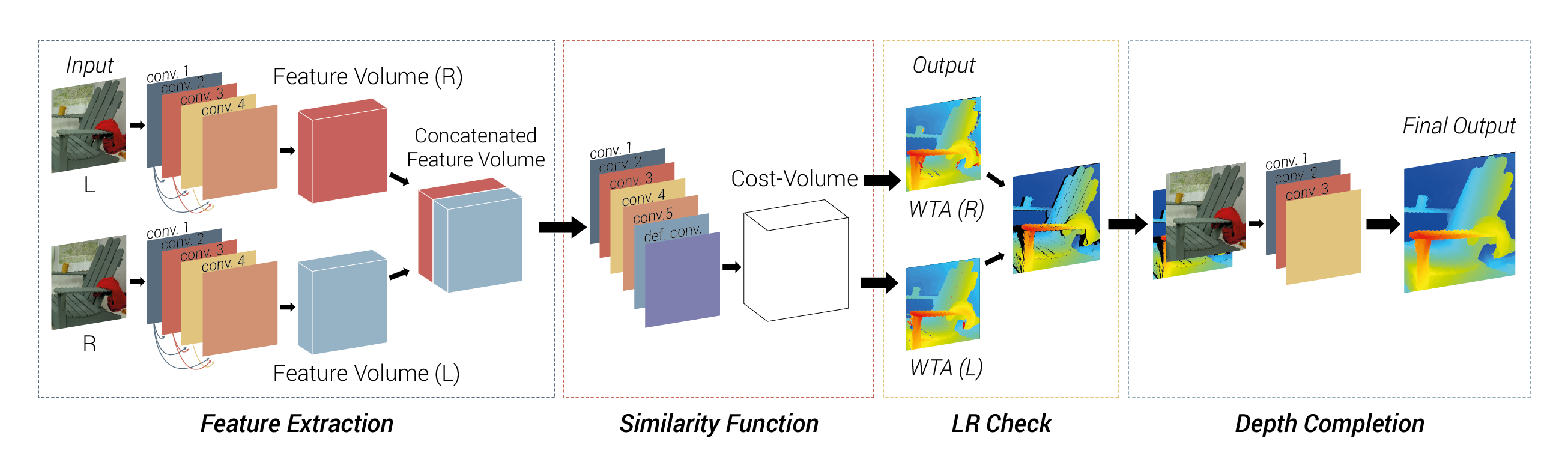
Figure 1: FCDSN-DC network structure. The Feature Extraction part learns expressive, deep features for the left and right image. Afterwards the Similarity Function part takes the concatenated input of the feature extractor and learns accurate similarity functions. Then the LR check is performed in order to get rid of inconsistent points. The Depth Completion part then takes the incomplete disparity map together with the corresponding RGB image in order to fill the missing disparity measurements.

I INTRODUCTION

Stereo vision has been a core problem of computer vision for many years. In stereo vision a pair of rectified images of the same scene but with different camera positions is used in order to extract 3D information. The retrieval of 3D information in such a manner is used in many important applications such as robotics, autonomous driving and 3D scene reconstruction. A traditional stereo method consists of four steps, namely: feature extraction, matching cost calculation, disparity estimation and disparity refinement. In the past all of this steps have been done using hand-crafted features and functions, however recent publications have shown real improvements upon this traditional methods, like SGM [1] or MGM [2] by replacing one or several steps using deep learning approaches.

The method FC-DCNN  [3] by D. Hirner and F. Fraundorfer is used as a baseline implementation for this method. There, it has been shown that replacing the feature extraction step with a deep learning approach in order to learn highly-dimensional and expressive features already outperforms traditional stereo methods such as SGM. We chose this method because of the lightweight and accurate foundation of the densely connected scheme that is easy to build upon. In this work we extend upon this method in two ways: Adding a network structure to learn a better similarity function between image patches and adding a network structure that learns to complete the sparse disparity map instead of using handcrafted post-processing steps. We end up with a fully trainable method that outperforms the baseline method of FC-DCNN [3] in all evaluated datasets and is comparable with other state-of-the art deep-learning methods. The whole method split into every step is illustrated in Fig. 1. We further show that this improvement in accuracy does not impact the generality of the method. We achieve all of this without the need of costly 3D-convolutions or fully-connected layers that are used by many popular state-of-the art methods such as GC-Net [4], PSMNet [5] or MC-CNN-acrt [6]. That 3D-convolutions are a major bottleneck for stereo estimation networks has been shown by R. Rahim et al. in their recent work [41].

The feature extraction part of our network consists of a densely-connected siamese CNN structure with shared weights. These highly-dimensional trained features of the left and right image are then concatenated and passed to the next part of the network in order to train a more accurate similarity function. This part of our method consists of five densely-connected layers with a deformable convolution block at the end in order to further improve the results. The feature extraction and the similarity function are trained jointly using a hinge-loss. These two trained parts are then used in order to create a cost-volume by writing the similarity measurement for each possible candidate at every possible image location along the predefined search direction and stacking them along the third dimension. This will lead to a cost-volume with the dimensions $H\times W\times D$, where $H$ and $W$ are the spatial dimensions of the image and $D$ is the maximum search range. Then a winner-takes-all approach is used by taking the argmax along the $D$ dimension in order to get the final disparity estimation. The disparity map for the left and the right image is created in such a manner and the left-right consistency check [7] is performed in order to remove inconsistent points.

The last part of the network then fills these previously removed inconsistent points. For each invalid point a set of consistent points is gathered along predefined cardinal directions. This gathered information together with the left RGB image is parsed into a shallow CNN network structure in order to train a new disparity label at this location. Instead of directly training on the integer ground-truth disparity we re-formulate the problem by choosing the closest disparity in the gathered information and using its position in the input vector as the class label.

This leads to a very lightweight network with a total of $0.385$ million trainable parameters, which is only $15$ thousand more than the baseline method FC-DCNN [3] and significantly less parameters than other machine learning stereo methods, which often need millions of trainable parameters. In summary, our contributions are as follows:

• We improve upon the baseline method FC-DCNN by adding two new parts, leading to a more accurate trainable method with two stages that outperforms the baseline method in every evaluated dataset.

• We introduce a novel yet simple machine learning method for depth completion. This method learns new disparities for previously considered inconsistent points with only the need of a shallow CNN structure. The output of this method is a completely dense and more accurate disparity map.

• We show that this method does not only outperform the baseline method on the most challenging and well-known stereo vision benchmarks, namely the Middlebury, Kitti and ETH3D benchmark, but can also compete with state-of-the art methods well known in the field.

• We show that our method is not only accurate for the trained datasets, but also applicable for a wide array of different domains without the need of retraining.

II Related Work

Our work is based on previous works on deep learning based stereo estimation networks, disparity refinement and depth completion.

Learning based stereo estimation has lead to some major advances in the field in recent years. J. Zbontar and Y. LeCun popularized the shared-weigths siamese network structure for stereo estimation in their work named MC-CNN [6]. In their work they extract small grayscale image patches from the left and the corresponding image patches from the right image. As their learning goal is to increase the distance of similarity between corresponding and non-corresponding image patches, they furthermore extract non-corresponding patches from the right image used for the training loss. J. Zbontar and Y. LeCun created two different versions of their method called MC-CNN-fast and MC-CNN-accurate. The first version uses the dot product as similarity function while the latter trains it using fully-connected layers. Most state-of the art learning based stereo methods use variations of the shared-weights siamese network structure [3][4][5][6][10][11][12][13][14].

In D. Hirner and F. Fraundorfers work called FC-DCNN [3] the siamese network structure was extended by using densely connected layers for the feature extractor as well as building a novel handcrafted post-processing method. In their paper they have shown that this hybrid method already works better than traditional methods such as SGM [1] while remaining lightweight in terms of the total number of trainable parameters.

H. Xu and J. Zhang introduced a network called AANet [13]. In this work they get completely rid of the 3D convolutions to achieve faster inference speed while maintaining comparable accuracy to other state-of the art methods. In their method they first use a feature extractor on multiple scales to create multiple cost-volumes on different scales. These cost-volumes are then passed to Intra- and Cross-Scale Aggregation modules. These modules use deformable convolutions [15][16] to get rid of edge-flattening issues. Afterwards the resulting disparity maps at different resolutions are used for upsampling and refinement.

Disparity refinement is used in order to further improve the disparity prediction. In this step the often noisy and outlier-prone initial disparity map is taken and improved via optimization. One of the most popular traditional disparity refinement methods is semi-global matching (SGM) by H. Hirschmueller [1]. In his paper he uses Mutual Information [17] as the similarity function in order to get the initial noisy disparity map. Afterwards the matching costs from all 16 cardinal direction for each pixel is aggregated and used in order to update the disparity value. This is done by viewing the aggregation of each direction separately as a 1D optimization problem which is then combined to get the updated value. G. Facciolo et al. [2] improved upon this method by using more evolved structures for the matching cost aggregation. In his paper he shows that these evolved structures can improve upon some artefacts of the belief update such as streaking artefacts that are often present when using the SGM [1] method.

Depth completion is the process of taking a sparse disparity input and assigning new values to the missing measurements. F. Aleotti et al. used monocular cues in their work [18] called Monocular Completion Network (MCN) in order to fill unreliable points. They argue that since monocular depth estimation does not rely on matching, it does not suffer from occlusion artefacts like traditional stereo methods. They leverage reliable disparity points gotten from a traditional stereo method and train a monocular disparity completion network on this. There exists a number of methods aiming to fill sparse depth maps based on the output of LIDAR scanners or SLAM algorithms [19][20][21][42][43]. These methods however are not directly comparable to our work, as they use depth or point cloud data directly as their input and therefore compete in different benchmarks.

III Network

The network consists of three sequentially dependent parts. First, rich and deep features are trained, then a similarity function for these new features is learned. In the last step, the left-right consistency check [7] is performed in order to get rid of inconsistent depth predictions and a novel trainable depth-completion task is performed to fill in this missing values. In our experiments, the feature extraction and similarity estimation part is trained jointly, while the depth-completion task is trained afterwards.

Our method differs from the baseline implementation FC-DCNN [3] in the following ways:

• The feature extractor remains the same, using densely connected fully-convolutional layers as proposed by G. Huang et al. [8]. Our feature extractor consists of four such densely connected convolutional layers training a 60 dimensional feature vector per image point. This is a reduction of one layer in comparison to the baseline method FC-DCNN [3]. We found this network configuration to work best through multiple empirical trial-and-error evaluations. The same training scheme is used as described in the baseline method implementation FC-DCNN [3], where the distance of the similarity score between matching and close non-matching image patches of the left and right image are increased by using a hinge-loss.

• The handcrafted cosine similarity function is replaced by our similarity function network. By fitting the similarity function on the data by training, a better accuracy score can be achieved.

• The handcrafted post-processing step to fill in the inconsistent points is replaced by our novel shallow network for depth-completion.

Our whole method has been implemented using Python3, pytorch 1.2.0 [22] and Cuda 10.0. Furthermore, we use the OpenCV 4.2.0 [23] library for image manipulation. The feature extraction and similarity measurement part are trained jointly using the Adam optimizer [24] with a learning rate of $6.0\times 10^{-5}$, a batch-size of $100$ and a patch-size of $21$. The depth completion part is trained separately, with the weights of the feature extractor and similarity measurement network being frozen. We use Adam optimizer [24] with a learning rate of $6.0\times 10^{-6}$ and the Cross-entropy loss $CE$ for the training of the depth completion network as seen in Eq. 1. For the depth-completion part a batch-size of $1000$ and a patch-size of $7$ is used for training.

$$CE=-\sum P(X)log(P(X))$$ (1)

III-A Similarity Measurement

The goal of the similarity measurement network is to learn better matching costs for the dataset than for example the cosine similarity or sum of absolute difference/sum of squared difference (SAD/SSD) [9]. It consists of five densely connected fully convolutional layers and one deformable convolution layer at the end of the network.

In contrast to other popular methods we do not use fully connected layers or 3D-convolutions. Instead it uses a fully convolutional, densely connected network structure which leads to a less complex yet accurate network structure. Furthermore, this network structure allows for varying input image size.

The network is trained jointly with the feature extraction network, getting as input the concatenated trained features for $s_{+}=\{p,q_{pos}\}$ and $s_{-}=\{p,q_{neg}\}$, where $p$ denotes the image point of the left image and $q_{pos}$ and $q_{neg}$ denotes the correct and and incorrect match of the right image respectively. Therefore the same hyperparameters, such as patch size, batch size or optimizer are used in order to train both the feature extraction as well as the similarity measurement part of the method. Both similarities $s_{+}$ and $s_{-}$ are then used in each training step, using Eq. 2 as loss.

$$loss=max(0,0.2+s_{-}-s_{+}).$$ (2)

III-B Depth Completion

In order to find new labels for the missing points we train a shallow CNN network. To this end, finding new labels is defined as a classification problem. However, instead of defining the integer disparities of the ground-truth as the class labels and training on that directly, we instead re-formulate the problem. In our method, this consistent disparity map with often large holes of missing data is taken and for every point marked invalid, a set number of valid points from the neighbourhood is gathered. The amount of valid points gathered is a hyperparameter. We empirically found that 10 valid points per invalid pixel lead to good results. The valid points are always gathered along the same directions, the left and the right side of the inconsistent point consecutively, however the first valid point along any given direction could be further or closer depending on how many invalid points are next in that direction. Afterwards the ground truth disparity value at that position is taken and compared with the gathered information. The position of the closest disparity within the range of $[-2,2]$ in the so created vector is then taken and recorded as the class-label for the training task. This is illustrated in the first example of Fig. 2. The first line, class, shows the position of the input vector as the class label which will be used for training. The second line, input, shows a dummy example of gathered valid disparities for a given invalid point. The third line shows the true disparity of this invalid point and the last line shows the found class label used for training. The input vector is then searched for the occurrence of this true disparity. If no value is found within this range of the ground-truth, the point is discarded for the training process.

If the found class-label has multiple entries in the vector, the first occurrence is taken as the label. This is shown in the second example of Fig. 2. This however has the drawback, that lower classes are favoured and therefore are more likely to appear. To counter this class imbalance that can occur, the class weights are normalized previous to training.

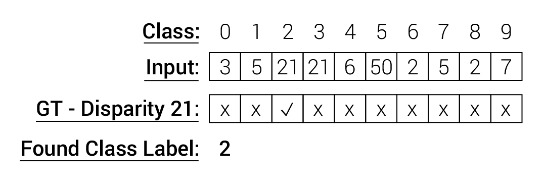
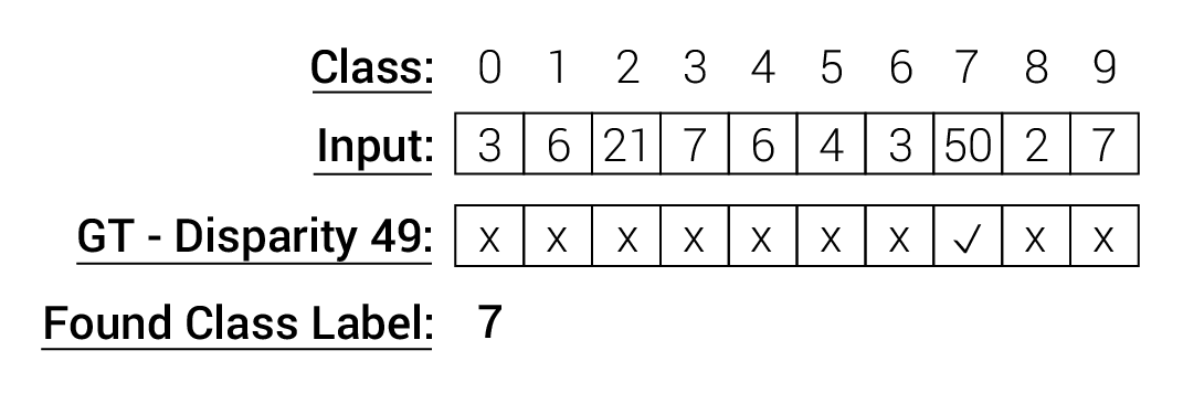
Figure 2: First: Example on how the ground-truth label for the depth-completion network is created given the collected valid disparities and the corresponding known disparity of the training dataset.
Second: Example on how the ground-truth label for the depth-completion network is created if the input vector has multiple valid entries.

A patch of the so created vectors together with the patch of RGB values of the left image at the same position is then taken as input for a shallow CNN. The network consists of three convolution layers and a softmax output layer.

This method has two main advantages over training the integer disparity labels directly: One, it strongly limits the number of classes needed for the classification task therefore also strongly limiting the needed resources and complexity of the network. Two, it helps with generalization as the disparity range of the data does not effect the input data, as only the position of the closest point in the neighbourhood is learned. One drawback of this method is that the data preparation for training and inference is more time-consuming as training directly on integer labels.

IV Experiments

We test our whole framework on a number of challenging real life indoor and outdoor scenes and compare our methods to the results of other state-of-the art methods from the official benchmarks with similar scores. For our overall ranking and further comparisons with more state-of-the art methods the online benchmarks can be visited.

IV-A Middlebury

The Middlebury stereo dataset [26] is a challenging indoor dataset with dense and highly accurate subpixel ground-truth data and an online leaderboard. All our experiments were done using the half (H) resolution.

Table I shows that we more than doubled the accuracy of the baseline method FC-DCNN on the training dataset in regards to the $4-PE$ and the $2-PE$ and strongly improved the $1-PE$. Furthermore we compare our results to other popular methods such as MC-CNN-acrt [6] or HSM-Net [29] and show that our method performs either better or is on-par with their results. The last row of Tab. I shows our results on the 13 additional samples of the 2014 Middlebury dataset that were not used in the training process.

TABLE I: Accuracy comparison on the Middlebury training dataset

Method	4-PE	2-PE	1-PE	0.5 PE
		Train
FCDSN-DC (ours)	5.08	9.47	26.6	60.6
LBPS [28]	4.97	9.63	21.2	51.5
MC-CNN-acrt [6]	6.34	10.1	18.4	39.8
HSM-Net_RVC [29]	4.52	10.2	22.8	49.2
FC-DCNN (baseline) [3]	12.3	17.9	34.7	65.1
		Test
FCDSN-DC (ours)	10.2	13.0	19.7	39.9

IV-B KITTI

KITTI stereo  [32] is an outdoor street image dataset created for autonomous driving. There are two different KITTI datasets, namely KITTI2012 and KITTI2015 captured in different years which can be viewed identical for the stereo estimation task.

Table II shows that we improved the accuracy of the baseline method with exception of the $2-PE$ for the KITTI2012 dataset. Although the method was optimized with the Middlebury dataset in mind, the method produces reasonable results that are on-par with, or better than other recently released learning based stereo methods and widely used non-learning methods such as the SGM implementation of OpenCV [23].

TABLE II: Accuracy comparison on the KITTI Testing dataset

Method	5-PE	4-PE	3-PE	2-PE
		KITTI2012
FCDSN-DC (ours)	3.16	3.80	5.11	9.11
FC-DCNN (baseline) [3]	3.71	4.40	5.61	8.81
OASM-Net [39]	4.32	5.11	6.39	9.01
AAFS [34]	3.28	4.28	6.10	10.64
HSMA [35]	5.13	6.20	8.15	13.44
		KITTI2015
FCDSN-DC (ours)	-	-	7.09	-
PASMnet [40]	-	-	7.23	-
AAFS [34]	-	-	7.54	-
FC-DCNN (baseline) [3]	-	-	7.71	-
OASM-Net [39]	-	-	8.98	-

IV-C ETH3D

The ETH3D stereo dataset [33] consists of a wide range of different indoor as well as outdoor scenes. Despite the fact, that this dataset is not the best fit for our method, as it has a small baseline and therefore less integer-valued disparities for training, Tab. III shows that we produce competitive results, often outperforming or being on-par with well-known machine learning based networks on the training dataset. The difference between the accuracy of the train and test dataset can be explained by looking closer at the individual samples. While the method works well for most test samples, a few samples produce high errors. This, in fact, is not due to overfitting of the method but rather these samples should be seen as failure cases for our method. The failure and success cases can be viewed at the official benchmark site of ETH3D. Despite that, Tab. III shows that our method outperforms the baseline method in all categories except the $0.5-PE$.

TABLE III: Accuracy comparison on the ETH dataset

Method	4-PE	2-PE	1-PE	0.5 PE
		Train
FCDSN-DC (ours)	0.45	0.70	1.58	11.37
HSM-Net_RVC [29]	0.37	0.88	2.86	10.31
RAFT-Stereo [30]	0.50	0.88	2.86	7.06
iResNet [31]	0.09	1.17	4.14	12.61
FC-DCNN (baseline) [3]	0.75	1.41	3.82	16.94
		Test
FCDSN-DC (ours)	2.66	5.04	10.24	25.59
HSM-Net_RVC [29]	0.52	1.40	4.20	10.88
RAFT-Stereo [30]	0.15	0.44	2.44	7.04
iResNet [31]	0.25	1.00	3.68	10.26
FC-DCNN (baseline) [3]	3.42	6.09	10.72	24.37

IV-D Ablation Study

In this section we show the validity and impact of our method by performing a number of ablation experiments. For the sake of consistency, all the following experiments are done using the same data, namely the Middlebury stereo dataset. To show the generality of the method, 13 image pairs from the 2014 Middlebury dataset were omitted from the training process and are used as the test split for all evaluations. The structure is as follows: First, we compare the accuracy of our trained similarity with the accuracy of the handcrafted cosine similarity cost. Next, we compare the accuracy of our trained similarity function with or without the deformable convolution layer. Last, we compare the accuracy of our method with and without the depth completion part.

IV-E Trained Similarity Function vs. Cosine

We show correctness and improvement of our trained similarity estimation function by conducting the following experiment. As the feature extraction and similarity estimation part are trained jointly, we train our feature extractor from scratch for one day using the cosine similarity. Afterwards the feature extraction and similarity estimation is trained jointly for the same amount of time in order to ensure fairness and correctness of the comparison.

TABLE IV: Ablation study trained similarity function on the test data

	4-PE	2-PE	1-PE	0.5-PE
		Train
Cosine	29.1795	32.946	39.251	57.328
Trained Similarity	15.793	19.350	30.234	55.584
		Test
Cosine	28.984	31.499	36.885	53.005
Trained Similarity	20.399	23.157	32.274	53.611

As Tab. IV shows, the accuracy of the method increases considerably when the similarity function is trained as opposed to using a handcrafted function such as cosine, except for the subpixel error on the test set.

IV-F Deformable Convolution Layer Ablation Study

We conduct an ablation study for the deformable convolution layer by running two experiments. First, we omit the last deformable convolution layer in the similarity estimation part of the network. For a more correct comparison we put a convolution-layer at the end with the same amount of trainable parameters as the deformable convolution layer has and train it for the same amount of training steps. Then, we repeat the experiment, only now with the deformable convolution layer in place. As seen in Tab. V, the deformable convolution layer improves the accuracy of the $4-PE$ and $2-PE$ but lowers the accuracy of the $1-PE$ and $0.5-PE$. This means that in our experiments, using a deformable convolutions decreases the lower end-point accuracy. However, our method is not build with subpixel accuracy in mind, instead focusing on optimizing the higher end-point errors. As the experiment shows an improvement in the higher end-point errors this does not speak against the use of deformable convolution layers.

TABLE V: Ablation study deformable convolution layer

	4-PE	2-PE	1-PE	0.5-PE
		Train
Without DConv	17.427	20.277	26.248	46.387
With DConv	15.793	19.350	30.234	55.584
		Test
Without DConv	21.717	23.991	29.161	46.258
With DConv	20.399	23.157	32.274	53.611

IV-G Depth Completion Ablation Study

In this section the validity and correctness of our depth completion part is shown. To this end we report on the disparity map result of the left frame with the depth completion part omitted and compare it with the depth completion in place.

TABLE VI: Ablation study depth completion (DC)

	4-PE	2-PE	1-PE	0.5-PE
		Train
Without DC	8.867	10.743	16.041	38.208
With DC	6.971	9.793	16.192	38.858
		Test
Without DC	16.272	18.288	23.858	42.533
With DC	10.240	13.025	19.681	39.860

Tab. VI shows that using our depth completion method improves upon the overall accuracy, especially for non-trained data.

IV-H Generalization Test

We show that our method generalizes well and is well suited for many different scenarios. We demonstrate this by using the hyperparameter and trained weights from the Middlebury dataset and do inference on true in-the-wild datasets that lack ground-truth or knowledge about the camera intrinsics. To this end we test our framework on two different publicly available datasets, namely the Holopix50k dataset [36] and the Flickr1024 dataset [37]. As Fig. 3 shows, our method produces useful results without the need of retraining for many different domains, such as indoor scenes with clutter, outdoor scenes and architecture. Furthermore, a quantitative study was performed to show the generality of the trained depth completion. To this end, we use the weights trained on one dataset, to do inference on the other datasets and report on the 2-point error. As input the disparity maps with removed inconsistencies produced by the previous parts of our method were taken.

TABLE VII: Generalization Test Depth Completion

	Middlebury	Kitti2012	Kitti2015	ETH3D
	(trained)	(trained)	(trained)	(trained)
Middlebury	9.47	10.254	11.02	10.256
Kitti2012	13.56	13.16	13.24	13.16
Kitti2015	15.58	15.21	15.21	15.21
ETH3D	0.93	0.87	0.98	0.87

Tab. VII shows the 2-PE of the quantitative generalization test of the depth completion part of our method. It shows that our method generalizes well and that the end-point error stays stable, even if the network is trained with different data.

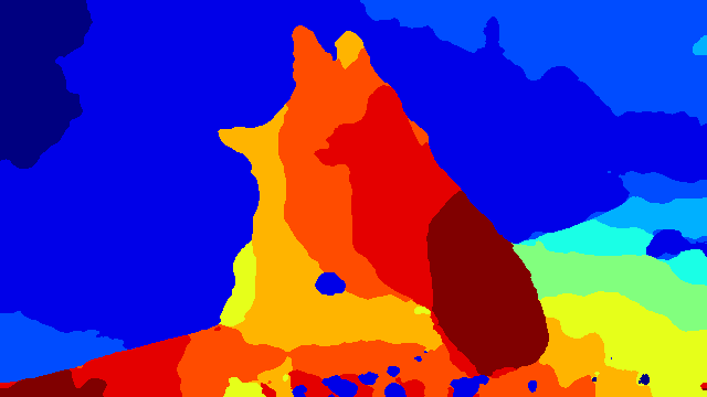
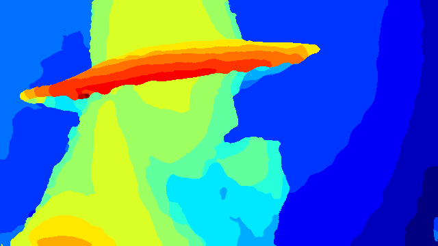
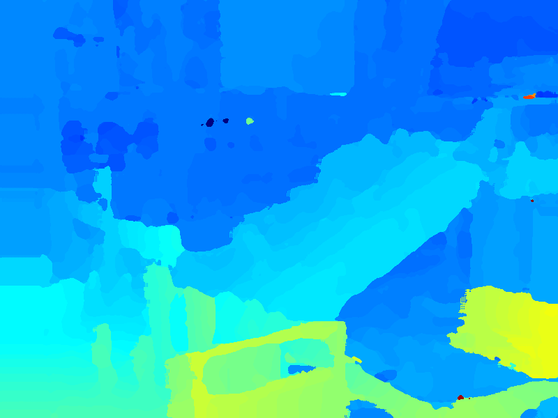
Figure 3: Qualitative results of selected stereo pair of our framework from different domains. From top to bottom: 2 samples of Holopix and 2 samples of Flickr.

V Conclusion

In this work we have presented a fully trainable stereo estimation method that produces completely dense disparity maps. We have shown that our method improved upon the baseline method of FC-DCNN in all evaluated challenging datasets. We have introduced a novel learning based depth-completion method. By reformulating the classification task for the missing disparity labels we were able to limit the amount of classes needed for inference and training for this task. We have argued that this leads to a shallow and effective network that improved the overall accuracy of the method. Furthermore, we have shown that our method is able to generalize well to previously unseen data from different domains, producing reasonable qualitative results.

References

- [1] H. Hirschmueller. Accurate and efficient stereo processing by semi-global matching and mutual information. IEEE Computer Society Conference on Computer Vision and Pattern Recognition (CVPR’05), Vol. 2., p. 807-814, 2005.
- [2] G. Facciolo, et al. MGM: A significantly more global matching for stereovision. BMVC 2015, 2015.
- [3] D. Hirner and F. Fraundorfer. FC-DCNN: A densely connected neural network for stereo estimation. 2020 25th International Conference on Pattern Recognition (ICPR). IEEE, 2021.
- [4] A. Kendall et al. End-to-end learning of geometry and context for deep stereo regression. Proceedings of the IEEE International Conference on Computer Vision, 2017.
- [5] J.R. Chang and Y.S. Chen. Pyramid stereo matching network. Proceedings of the IEEE Conference on Computer Vision and Pattern Recognition, 2018.
- [6] J. Zbontar and Y. LeCun. Stereo matching by training a convolutional neural network to compare image patches. Journal of Machine Learning Research, Vol. 17, p. 1-32, 2016.
- [7] C. Chang et al. On an analysis of static occlusion in stereo vision. IEEE Computer Society Conference on Computer Vision and Pattern Recognition, p.722-723, 1991.
- [8] G. Huang et al. Densely connected convolutional networks. Proceedings of the IEEE conference on computer vision and pattern recognition, 2017.
- [9] D. Kong and H. Tao. A Method for Learning Matching Errors in Stereo Computation. BMVC, p. 2, 2004.
- [10] P. Knobelreiter et al. End-to-end training of hybrid CNN-CRF models for stereo. Proceedings of the IEEE Conference on Computer Vision and Pattern Recognition, 2017.
- [11] F. Zhang et al. Ga-net: Guided aggregation net for end-to-end stereo matching. Proceedings of the IEEE Conference on Computer Vision and Pattern Recognition, 2019.
- [12] W. Luo et al. Efficient deep learning for stereo matching. Proceedings of the IEEE Conference on Computer Vision and Pattern Recognition, 2016.
- [13] H. Xu and J. Zhang. Aanet: Adaptive aggregation network for efficient stereo matching. Proceedings of the IEEE/CVF Conference on Computer Vision and Pattern Recognition, p.1959–1968, 2020.
- [14] L. Lipson et al. RAFT-Stereo: Multilevel Recurrent Field Transforms for Stereo Matching. arXiv preprint arXiv:2109.07547, 2021.
- [15] J. Dai et al.Deformable convolutional networks. Proceedings of the IEEE international conference on computer vision, p.764–773,2017
- [16] X. Zhu et al. Deformable convnets v2: More deformable, better results. Proceedings of the IEEE/CVF Conference on Computer Vision and Pattern Recognition, p. 9308–9316, 2019.
- [17] P. Viola and W.M. Wells III. Alignment by maximization of mutual information. International journal of computer vision 24.2, p. 137-154, 1997.
- [18] F. Aleotti et al. Reversing the cycle: self-supervised deep stereo through enhanced monocular distillation. European Conference on Computer Vision, p.614–632, 2020.
- [19] A. Eldesokey et al. Propagating confidences through cnns for sparse data regression. arXiv preprint arXiv:1805.11913, 2018.
- [20] J. Ku et al. In defense of classical image processing: Fast depth completion on the cpu. 2018 15th Conference on Computer and Robot Vision (CRV). IEEE, 2018.
- [21] L.K. Liu et al. Depth reconstruction from sparse samples: Representation, algorithm, and sampling. IEEE Transactions on Image Processing 24.6 , p.1983-1996, 2015.
- [22] A. Paszke et al. PyTorch: An Imperative Style, High-Performance Deep Learning Library. Advances in Neural Information Processing Systems 32, p. 8024–8035, 2019.
- [23] G. Bradski. Open Source Computer Vision Library. Dr. Dobb’s journal of software tools 3, 2000.
- [24] D.P. Kingma and J.Ba. Adam: A method for stochastic optimization. arXiv preprint arXiv:1412.6980, 2014.
- [25] H. Wu et al. Fast end-to-end trainable guided filter. Proceedings of the IEEE Conference on Computer Vision and Pattern Recognition, 2018.
- [26] D. Scharstein et al. High-resolution stereo datasets with subpixel-accurate ground truth. German conference on pattern recognition. Springer, Cham, 2014.
- [27] A. Wong et al. An Adaptive Framework for Learning Unsupervised Depth Completion. IEEE Robotics and Automation Letters, 6.2, p.3120–3127, 2021.
- [28] P.Knöbelreiter et al. Belief Propagation Reloaded: Learning BP-Layers for Labeling Problems. Proceedings of the IEEE/CVF Conference on Computer Vision and Pattern Recognition, p.7900–7909, 2020.
- [29] G. Yang et al. Hierarchical deep stereo matching on high-resolution images. Proceedings of the IEEE/CVF Conference on Computer Vision and Pattern Recognition, p.5515–5524, 2019.
- [30] L. Lipson et al. Raft-stereo: Multilevel recurrent field transforms for stereo matching. arXiv preprint arXiv:2109.07547, 2021.
- [31] Z. Liang et al. Learning for disparity estimation through feature constancy. Proceedings of the IEEE Conference on Computer Vision and Pattern Recognition, p.2811–2820, 2018.
- [32] M. Menze and A. Geiger. Object scene flow for autonomous vehicles. Proceedings of the IEEE conference on computer vision and pattern recognition., 2015.
- [33] Thomas Schöps et al. A Multi-View Stereo Benchmark with High-Resolution Images and Multi-Camera Videos. Proceedings of the IEEE Conference on Computer Vision and Pattern Recognition, 2017.
- [34] J. Chang et al. Attention-Aware Feature Aggregation for Real-time Stereo Matching on Edge Devices. Proceedings of the Asian Conference on Computer Vision, 2020.
- [35] O. Zeglazi et al. A hierarchical stereo matching algorithm based on adaptive support region aggregation method. Pattern Recognition Letters 112, p.205-211, 2018.
- [36] Y. Hua et al. Holopix50k: A large-scale in-the-wild stereo image dataset. arXiv preprint arXiv:2003.11172, 2020.
- [37] Y. Wang et al. Flickr1024: A large-scale dataset for stereo image super-resolution. Proceedings of the IEEE/CVF International Conference on Computer Vision Workshops, 2019.
- [38] J. Zhang et al. Dispsegnet: Leveraging semantics for end-to-end learning of disparity estimation from stereo imagery. IEEE Robotics and Automation Letters 4.2, p.1162-1169, 2019.
- [39] L. Ang and Y. Zejian. Occlusion Aware Stereo Matching via Cooperative Unsupervised Learning. Proceedings of the Asian Conference on Computer Vision, ACCV, 2018.
- [40] L. Wang et al. Parallax attention for unsupervised stereo correspondence learning. IEEE transactions on pattern analysis and machine intelligence, 2020.
- [41] R. Rahim et al. Separable convolutions for optimizing 3d stereo networks., 2021 IEEE International Conference on Image Processing, ICIP, 2021.
- [42] F. Ma and S. Karaman. Sparse-to-dense: Depth prediction from sparse depth samples and a single image., 2018 IEEE international conference on robotics and automation (ICRA), 2018.
- [43] F. Ma et al. Self-supervised sparse-to-dense: Self-supervised depth completion from lidar and monocular camera., 2019 International Conference on Robotics and Automation (ICRA), 2019.