Quantum critical behaviors and decoherence of weakly coupled
quantum Ising models within an isolated global system

Abstract

We discuss the quantum dynamics of an isolated composite system consisting of weakly interacting many-body subsystems. We focus on one of the subsystems, ${\cal S}$, and study the dependence of its quantum correlations and decoherence rate on the state of the weakly-coupled complementary part ${\cal E}$, which represents the environment. As a theoretical laboratory, we consider a composite system made of two stacked quantum Ising chains, locally and homogeneously weakly coupled. One of the chains is identified with the subsystem ${\cal S}$ under scrutiny, and the other one with the environment ${\cal E}$. We investigate the behavior of ${\cal S}$ at equilibrium, when the global system is in its ground state, and under out-of-equilibrium conditions, when the global system evolves unitarily after a soft quench of the coupling between ${\cal S}$ and ${\cal E}$. When ${\cal S}$ develops quantum critical correlations in the weak-coupling regime, the associated scaling behavior crucially depends on the quantum state of ${\cal E}$, whether it is characterized by short-range correlations (analogous to those characterizing disordered phases in closed systems), algebraically decaying correlations (typical of critical systems), or long-range correlations (typical of magnetized ordered phases). In particular, different scaling behaviors, depending on the state of $\cal E$, are observed for the decoherence of the subsystem ${\cal S}$, as demonstrated by the different power-law divergences of the decoherence susceptibility that quantifies the sensitivity of the coherence to the interaction with ${\cal E}$.

I Introduction

The recent progress on the nano-scale control of physical systems has opened the road to investigations of the quantum properties and of the coherent quantum dynamics of coupled systems, addressing also issues concerning the relative decoherence and the energy flow among the various subsystems Zurek-03 . These investigations improve our understanding of the emergence of interference and entanglement, which is useful for quantum-information purposes NielsenChuang , or for enhancing the efficiency of energy conversion in complex networks Lambert-13 . The presence of different quantum phases and the development of critical behaviors in interacting subsystems are expected to play a crucial role for the emergence of new phenomena in the equilibrium and out-of-equilibrium dynamics of isolated and open quantum systems Sachdev-book ; RV-21 .

If we consider a quantum system made up of various components, any subsystem can be seen as an effective bath for the other ones. In this context, one may study the quantum dynamics of an open system subject to the interaction with the environment, while the global system (composed of the open system and its environment) evolves unitarily. These issues have been already addressed within some paradigmatic, relatively simple, composite models, such as the so-called central-spin models, where one or few qubits are globally coupled to an environmental many-body system Zurek-82 ; CPZ-05 ; QSLZS-06 ; RCGMF-07 ; CFP-07 ; CP-08 ; Zurek-09 ; DQZ-11 ; NDD-12 ; SND-16 ; V-18 ; FCV-19 ; RV-19 ; RV-21 , and sunburst models where sets of isolated qubits are locally coupled to a many-body system FRV-22 ; FRV-22-2 . The decoherence properties of the subsystems crucially depend on the large-scale features of the state they are in, for instance, on whether the subsystem is in an ordered or a disordered quantum phase, or it is close to a critical point, where large-scale critical correlations develop Sachdev-book .

In this paper we focus on the open dynamics of one many-body subsystem ${\cal S}$ weakly coupled with a complementary environment ${\cal E}$. We study the dependence of the critical behavior of ${\cal S}$ on the coupling between ${\cal S}$ and ${\cal E}$, and on the state of the environment ${\cal E}$, which can be controlled by varying the Hamiltonian parameters.

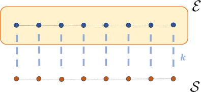
Figure 1: Sketch of a system made of two stacked Ising chains, weakly coupled by local and homogenous interactions controlled by a parameter $\kappa$. One of the chains represents the subsystem ${\cal S}$, while the other is the environment ${\cal E}$.

As a theoretical laboratory, we consider two stacked one-dimensional Ising chains, locally and homogeneously weakly coupled, as sketched in Fig. 1. One of the chains represents the subsystem ${\cal S}$, the other one is the environment ${\cal E}$. The Hamiltonian parameters of the two chains (for example, the Hamiltonian coefficient of the external transverse field) differ, so that ${\cal S}$ and ${\cal E}$ may be in different quantum phases. We discuss how a weak interaction between ${\cal S}$ and ${\cal E}$ (controlled by one parameter $\kappa$ that vanishes when ${\cal S}$ and ${\cal E}$ are decoupled) affects the quantum scaling behaviors and the decoherence rate of ${\cal S}$, close to critical transitions. We discuss static properties, assuming that the global system is in its ground state, and the out-of-equilibrium behavior when a slow quench of the interactions between ${\cal S}$ and ${\cal E}$ is performed. We show that the scaling behavior in the weak-coupling regime depends on the quantum state of ${\cal E}$. More precisely, a disordered, critical, ordered environment, characterized by short-range, algebraically decaying, and long-range correlations, respectively, differently affects the critical scaling behavior of $\cal S$.

To characterize the scaling behavior in the presence of a coupling between ${\cal S}$ and ${\cal E}$ controlled by a parameter $\kappa$, we use the renormalization-group (RG) approach, which provides the natural theoretical framework to effectively describe the behavior of systems in proximity of quantum transitions, see, e.g., Refs. Sachdev-book ; RV-21 . We focus, in particular, on the large-size behavior of the system, deriving finite-size scaling (FSS) relations, which are largely independent of the microscopic details. Therefore, they hold in widely different systems and in very different physical contexts. Moreover, they allow us to describe complex phenomena using a relatively small number of relevant variables, providing a notable simplification of the analysis.

As we mentioned above, in the presence of a coupling between $\cal S$ and $\cal E$, some features of the critical behavior of $\cal S$ depend on whether $\cal E$ is disordered, critical, or ordered. For instance, the sensitivity of the coherence properties of $\cal S$ to the coupling strength $\kappa$ is significantly different in these three cases. Such a sensitivity can be effectively quantified by using the the susceptibility $\chi_{Q}$ of the decoherence factor of ${\cal S}$ with respect to the parameter $\kappa$, since this quantity shows a different power-law divergence with the size $L$ of the system in the three cases mentioned above. The RG predictions derived in this work have been confirmed by the FSS analysis of numerical results for stacked Ising chains.

In a dynamic perspective, the study of the phase diagram and of the scaling properties of the global system determines the adiabatic limit of a slow dynamics for a finite-size system (we recall that finite-size many-body systems are generally gapped). We also extend the discussion to out-of-equilibrium conditions, determining the effects of an instantaneous quench of the coupling between ${\cal S}$ and ${\cal E}$. Again we use a RG framework, deriving general dynamic FSS relations that extend those obtained for the system in equilibrium.

The paper is organized as follows. In Sec. II we define the system we consider, composed of two coupled (stacked) $d$-dimensional quantum Ising systems. In Sec. III we introduce the observables we use to characterize the critical properties of the subsystem ${\cal S}$. In Sec. IV we derive general FSS relations that characterize the equilibrium behavior of the subsystem ${\cal S}$ in the presence of a weak coupling with the environment ${\cal E}$. The different RG scaling ansätze, which depend on the quantum phase of the environment, are supported by numerical results for coupled quantum Ising chains. In Sec. V we discuss the general features of the phase diagram for finite values of the coupling $\kappa$ between ${\cal S}$ and ${\cal E}$. In Sec. VI we extend the discussion to out-of-equilibrium dynamic processes, considering a soft quench of the interaction between ${\cal S}$ and ${\cal E}$. Finally, in Sec. VII we summarize and draw our conclusions. App. A provides a mean-field analysis of the phase diagram of stacked Ising systems. App. B reports exact results in some limiting cases.

II Coupled quantum Ising systems

We consider a system composed of two interacting (stacked) $d$-dimensional quantum Ising models: one of them is identified as the subsystem ${\cal S}$ under observation and the other one as the environment ${\cal E}$. The Hamiltonian of the global system is

$$H=H_{\cal S}(J,g)+H_{\cal E}(J_{e},g_{e})+H_{\cal SE}(\kappa)\,,$$ (1)

where

$$H_{\cal S}(J,g)=-J\sum_{\langle{\bm{x}}{\bm{y}}\rangle}\sigma^{(1)}_{{\bm{x}}}\sigma^{(1)}_{{\bm{y}}}-g\sum_{\bm{x}}\sigma^{(3)}_{{\bm{x}}}\,,$$ (2)

$$H_{\cal E}(J_{e},g_{e})=-J_{e}\sum_{\langle{\bm{x}}{\bm{y}}\rangle}\tau^{(1)}_{{\bm{x}}}\tau^{(1)}_{{\bm{y}}}-g_{e}\sum_{\bm{x}}\tau^{(3)}_{{\bm{x}}}\,,$$ (3)

$$H_{\cal SE}(\kappa)=-\kappa\,\sum_{\bm{x}}\sigma^{(1)}_{{\bm{x}}}\tau^{(1)}_{{\bm{x}}}\,,$$ (4)

where ${\bm{x}}$ are the sites of a cubic-like lattice of size $L^{d}$, ${\langle{\bm{x}}{\bm{y}}\rangle}$ indicates nearest-neighbor sites, $\sigma^{(k)}_{\bm{x}}$ and $\tau^{(k)}_{\bm{x}}$ are two independent sets of Pauli matrices. In the following we consider generic boundary conditions, for example open or periodic boundary conditions (OBC and PBC, respectively). The coupling $\kappa$ controls the strength of the interactions between the subsystems ${\cal S}$ and ${\cal E}$, while the Hamiltonian parameters $J_{e}$ and $g_{e}$ allow us to control the quantum state of the environment (in the regime of weak coupling between ${\cal S}$ and ${\cal E}$). To reduce the number of input parameters, we set

$$J=J_{e}=1\,,$$ (5)

which does not limit the generality of our discussion (unless one is interested in some particular limits that we do not consider). For $d=1$ we obtain the stacked Ising chains sketched in Fig. 1.

For $\kappa=0$, the system is invariant under the ${\mathbb{Z}}_{2}\otimes{\mathbb{Z}}_{2}$ group of transformations that independently change the signs of the $\sigma^{(1)}_{\bm{x}}$ and $\tau_{\bm{x}}^{(1)}$ operators. The interaction Hamiltonian $H_{\cal SE}$ breaks this invariance, leaving only a global ${\mathbb{Z}}_{2}$ symmetry under the simultaneous transformations

$$\sigma^{(1/2)}_{\bm{x}}\to-\sigma^{(1/2)}_{\bm{x}}\,,\qquad \sigma^{(3)}_{\bm{x}}\to\sigma^{(3)}_{\bm{x}}\,,$$

$$\tau^{(1/2)}_{\bm{x}}\to-\tau^{(1/2)}_{\bm{x}}\,,\qquad \tau^{(3)}_{\bm{x}}\to\tau^{(3)}_{\bm{x}}\,.$$

Note that, if we only change the sign of one the longitudinal spin operators, i.e., $\sigma^{(1)}_{\bm{x}}\to-\sigma^{(1)}_{\bm{x}}$ or $\tau^{(1)}_{\bm{x}}\to-\tau^{(1)}_{\bm{x}}$, we obtain the same Hamiltonian with $\kappa$ replaced by $-\kappa$. Thus, the phase diagram does not depend on the sign of $\kappa$. Without loss of generality, we assume $\kappa\geq 0$. Moreover, at fixed $\kappa$, the phase diagram of the global system is invariant under the exchange $g\leftrightarrow g_{e}$, due to the fact that the two subsystems ${\cal S}$ and ${\cal E}$ are identical apart from their transverse-field parameters $g$ and $g_{e}$.

A simplified model is obtained for $g=g_{e}$. In this case, the global system has an additional ${\mathbb{Z}}_{2}$ symmetry, as it is invariant under the interchange $\sigma_{\bm{x}}\leftrightarrow\tau_{\bm{x}}$. Thus, the symmetry group enlarges to ${\mathbb{Z}}_{2}\otimes{\mathbb{Z}}_{2}\otimes{\mathbb{Z}}_{2}$ for $\kappa=0$ and to ${\mathbb{Z}}_{2}\otimes{\mathbb{Z}}_{2}$ when the two systems are coupled ($\kappa\not=0$).

It is worth noting that the symmetry properties of the global system change, if the coupling Hamiltonian involves the transverse spin operators, i.e., if $H_{\cal SE}$, defined in Eq. (4), is replaced by

$$\widetilde{H}_{\cal SE}=-\widetilde{\kappa}\sum_{\bm{x}}\sigma^{(3)}_{{\bm{x}}}\tau^{(3)}_{{\bm{x}}}\,,$$ (7)

where $\widetilde{\kappa}$ is the parameter controlling the strength of the interaction. Indeed, such a coupling term preserves the ${\mathbb{Z}}_{2}\otimes{\mathbb{Z}}_{2}$ symmetry present for $\widetilde{\kappa}=0$. Note that, in the symmetric case $g=g_{e}$, the global model with the interacting term $\widetilde{H}_{\cal SE}$ is equivalent to the so-called quantum Ashkin-Teller model, see, e.g., Refs. Fradkin-84 ; Shankar-85 . In this paper we only consider models coupled through their longitudinal spin operators, such as in Eq. (4), breaking the independent ${\mathbb{Z}}_{2}$ invariance of the two subsystems. The alternative case, corresponding to the coupling $\widetilde{H}_{\cal SE}$, is also worth investigating, as it would provide insights on the quantum dynamics, when the interaction term between ${\cal S}$ and ${\cal E}$ does not break any symmetry of the isolated system. We do not pursue it in this paper.

When the interaction between the subsystems vanishes, i.e., when $\kappa=0$, one recovers two decoupled $d$-dimensional quantum Ising systems. Therefore, it is useful to recall that $d$-dimensional quantum Ising systems, described by the Hamiltonian (2) supplemented by an additional longitudinal term $H_{h}=-h\sum_{\bm{x}}\sigma_{\bm{x}}^{(1)}$, undergo a quantum continuous transition at a finite value $g=g_{\cal I}$ and $h=0$; see, e.g., Ref. Sachdev-book ; RV-21 . The corresponding quantum critical behavior belongs to the $(d+1)$-dimensional Ising universality class. In particular, we have $g_{\cal I}=1$ for the one-dimensional Ising chain. The relevant parameters $r\equiv g-g_{\cal I}$ and $h$, associated with the transverse and longitudinal spin operators $\sigma_{\bm{x}}^{(3)}$ and $\sigma_{\bm{x}}^{(1)}$, represent the leading even and odd RG perturbations at the $(d+1)$-dimensional Ising fixed point. Their RG dimensions are $y_{r}=1/\nu$ and $y_{h}$, respectively, so that the length scale $\xi$ of the critical modes behaves as $\xi\sim|g-g_{\cal I}|^{-\nu}$ for $h=0$, and $\xi\sim|h|^{-1/y_{h}}$ for $g=g_{\cal I}$. The RG exponents are exactly known for one-dimensional systems: $y_{r}=1$ and $y_{h}=15/8$, see, e.g., Ref. Sachdev-book . Accurate estimates are available for two-dimensional quantum Ising systems, see, e.g., Refs. PV-02 ; GZ-98 ; CPRV-02 ; Hasenbusch-10 ; KPSV-16 ; KP-17 ; Hasenbusch-21 ; Ref. KPSV-16 reports $y_{r}=1.58737(1)$ and $y_{h}=2.481852(1)$. For $d=3$, the critical exponents take their mean-field values, $y_{r}=2$ and $y_{h}=3$; moreover, the critical singular behavior is characterized by additional multiplicative logarithmic factors Sachdev-book ; RV-21 ; PV-02 . The dynamic exponent $z$, controlling the vanishing of the gap $\Delta\sim\xi^{-z}$ at the transition point, is 1 in any dimension. For later use, we recall that the RG dimension $y_{\phi}$ of the longitudinal spin operator $\sigma_{x}^{(1)}$ (it represents the order parameter of the model) is given by $y_{\phi}=d+z-y_{h}=(d+z-2+\eta)/2$, where $\eta$ is the critical exponent characterizing the spatial decay of the critical correlations. Using the above-reported results for $y_{h}$, we have $y_{\phi}=1/8$ for $d=1$, $y_{\phi}=0.518148(1)$ for $d=2$, and $y_{\phi}=1$ for $d=3$.

III Observables at equilibrium

To study the equilibrium properties of the subsystem ${\cal S}$ when the global system is in the ground state $|\Psi_{0}\rangle$, considering ${\cal E}$ as the environment, we introduce the reduced density matrix of ${\cal S}$

$$\rho_{\cal S}={\rm Tr}_{\cal E}\,\big{[}|\Psi_{0}\rangle\langle\Psi_{0}|\big{]}\,,$$ (8)

where ${\rm Tr}_{\cal E}[\,\cdot\,]$ denotes the partial trace over the Hilbert space associated with the subsystem ${\cal E}$.

The coherence properties of ${\cal S}$ can be quantified through the purity $P$, the corresponding Rényi entanglement entropy $S$, and the decoherence factor $Q$, defined as

$$P={\rm Tr}\big{[}\rho_{\cal S}^{2}\big{]}\,,\qquad S=-{\rm ln}\,P\,,\qquad Q=1-P\,.$$ (9)

Exploiting the Schmidt decomposition for bipartitions of pure states, one can easily prove that the purity $P$ of the subsystem ${\cal S}$ equals that of the complementary environment ${\cal E}$. The decoherence factor varies between zero (corresponding to $P=1$ and $S=0$, for a pure reduced state) and 1 (corresponding to $P=0$, for a completely incoherent many-body state).

To quantify the loss of coherence of the subsystem ${\cal S}$ due to a weak interaction term $H_{\cal SE}$, we look at the behavior of $Q$ for small values of $\kappa$. Since $Q$ is an even function of $\kappa$, assuming analyticity at $\kappa=0$ (which is certainly true for finite-size systems), we can expand it as

$$Q={1\over 2}\kappa^{2}\chi_{Q}+O(\kappa^{4})\,,\qquad\chi_{Q}\equiv{\partial^{2}Q\over\partial\kappa^{2}}\bigg{|}_{\kappa=0}\,,$$ (10)

where $\chi_{Q}$ represents the decoherence susceptibility with respect to the coupling $\kappa$.

We also consider the correlations of the spin operators $\sigma_{x}^{(1)}$. Due to the global ${\mathbb{Z}}_{2}$ symmetry, we have

$${\rm Tr}\big{[}\rho_{\cal S}\,\sigma_{\bm{x}}^{(1)}\big{]}=0\,.$$ (11)

The two-point correlation function can be written as

$$G({\bm{x}},{\bm{y}})\equiv{\rm Tr}\big{[}\rho_{\cal S}\,\sigma_{\bm{x}}^{(1)}\sigma_{\bm{y}}^{(1)}\big{]}\,.$$ (12)

We consider odd values of $L$, we set $L=2\ell+1$, and choose coordinates such that $-\ell\leq x_{i}\leq\ell$, so that we can identify a central site ${\bm{x}}_{0}$ with vanishing coordinates (this coordinate system is particularly convenient in the case of OBC). We consider a susceptibility and second-moment correlation length, defined as

$$\chi=\sum_{\bm{x}}G({\bm{x}}_{0},{\bm{x}})\,,\quad\xi^{2}={1\over 2d\chi}\sum_{\bm{x}}{\bm{x}}^{2}G({\bm{x}}_{0},{\bm{x}})\,.$$ (13)

The ratio

$$R_{\xi}=\xi/L$$ (14)

is a RG invariant quantity. In the FSS limit, it scales as $R_{\xi}(g,L)\approx{\cal R}(rL^{y_{r}})$, where $r=g-g_{\cal I}$ and ${\cal R}$ is a function that is universal apart from a rescaling of its argument PV-02 ; CPV-14 . Moreover, the susceptibility $\chi$ behaves as $\chi\approx\,L^{d-2y_{\phi}}{\cal C}(rL^{y_{r}})$, where $d-2y_{\phi}=2-z-\eta=1-\eta$, or, equivalently, as

$$\chi\approx L^{1-\eta}a_{\chi}F_{\chi}(R_{\xi})\,.$$ (15)

The function $F_{\chi}(R_{\xi})$ is universal, while $a_{\chi}$ is a nonuniversal constant that depends on the model parameters.

IV Scaling behaviors for weakly coupled subsystems

We now discuss how the coupling term $H_{\cal SE}$ affects the quantum critical properties of ${\cal S}$ for small values of $\kappa$. Using RG arguments, we show that ${\cal S}$ develops different scaling behaviors, that depend on the state of the environment ${\cal E}$, controlled by the Hamiltonian parameter $g_{e}$, cf. Eq. (3). We refer here to the state of $\cal E$ for $\kappa=0$. Indeed, the addition of a coupling term $H_{\cal SE}$ also changes the properties of the environment. We distinguish three cases: (i) the environment ${\cal E}$ is disordered, $g_{e}>g_{\cal I}$; (ii) ${\cal E}$ is in the critical regime, $g_{e}\approx g_{\cal I}$; (iii) the environment is ordered (magnetized), i.e., $g_{e}<g_{\cal I}$.

The predicted scaling behaviors will be compared with the results of numerical FSS analyses for the one-dimensional model (1), i.e., for two stacked Ising chains, sketched in Fig. 1. To compute correlation functions, we use the density-matrix RG (DMRG) algorithm with OBC, which allows us to obtain results for systems of size up to $L\approx 40$. As for the implementation, we use matrix-product-state (MPS) algorithms taken from the iTensor library FWS-20 . The DMRG algorithm is very convenient to compute coherence properties for left-right bipartitions of the system. In principle, it could also be used to compute $Q$ in our case, by considering $\cal S$ and $\cal E$ as the left and right ordering of the ladder model that we consider. However, in this type of implementation, one would generate nonlocal interactions between the two subsystems, making the algorithm inefficient. Therefore, the decoherence factor $Q$ has been computed by performing an exact diagonalization of the global Hamiltonian. Of course, smaller systems can be considered (we obtained results up $L\approx 10$). In this case we used PBC.

IV.1 Disordered environment

Let us first assume that the environment ${\cal E}$ is disordered for $\kappa=0$. It presents only short-range correlations, so that it may be effectively considered as a collection of a large number of independent subsystems. For an Ising system, such as the one described by the Hamiltonian (3), the environment ${\cal E}$ is disordered for $g_{e}>g_{\cal I}$. We focus on the subsystem ${\cal S}$, and, in particular, on the scaling behavior of its decoherence properties for small values of the coupling $\kappa$.

IV.1.1 Scaling behavior for small $\kappa$

For $g_{e}>g_{\cal I}$, we conjecture that the interaction $H_{\cal SE}$ between ${\cal S}$ and ${\cal E}$ is an irrelevant perturbation at the quantum critical point of the subsystem ${\cal S}$. Under this hypothesis, the subsystem ${\cal S}$ has an Ising critical transition also for finite $\kappa$, at a critical point $g_{c}(\kappa)$ that depends on $\kappa$. Since the coupling $\kappa$ is irrelevant, there is only one relevant operator also for $\kappa\not=0$. We indicate the corresponding scaling field with $u_{r}$ ($u_{r}\sim r$ in the absence of coupling $\kappa$). Its RG dimension $y_{r}$ is the same as that of the thermal operator in the Ising universality class, see at the end of Sec. II.

We recall that the scaling fields associated with the RG perturbations are analytic functions of the model parameters Wegner-76 ; PV-02 ; CPV-14 ; RV-21 . In the case at hand, in which there is only one relevant RG perturbation, the singular part of the free-energy density in the zero-temperature and FSS limit is expected to scale as CPV-14 ; RV-21

$$F_{\rm sing}(g,g_{e}>g_{\cal I},\kappa,L)\approx L^{-(d+z)}{\cal F}(W_{s})\,,$$ (16)

where

$$W_{s}=u_{r}L^{y_{r}}\,.$$ (17)

Correspondingly, any RG invariant quantity $R$, such as $R_{\xi}$ defined in Eq. (14) or the decoherence factor $Q$ defined in Eq. (9), is expected to asymptotically scale as CPV-14

$$R\approx F_{R}(W_{s})\,.$$ (18)

The scaling field $u_{r}$ is an analytic function of $g$, $\kappa$, and $g_{e}$, such that $u_{r}\sim r$ for $\kappa=0$. Due to the symmetry of the phase diagram under $\kappa\to-\kappa$, for small values of $r$ and $\kappa$ it behaves as

$$u_{r}(r,\kappa)\approx r+b\,\kappa^{2}\,,\qquad r=g-g_{\cal I}\,,$$ (19)

where the nonuniversal constant $b$ depends on the environment coupling $g_{e}$, and we fixed an arbitrary normalization requiring $u_{r}\approx r$ for $\kappa=0$.

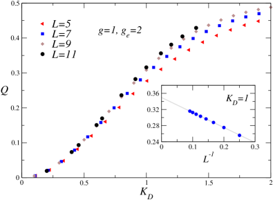
Figure 2: Scaling behavior of the decoherence factor $Q$ for the critical Ising chain ($g=1$), coupled with a disordered environment ($g_{e}=2$), versus $K_{D}=\kappa L^{1/2}$. PBC are used. The results are consistent with the scaling relation (20). The inset shows data at fixed $K_{D}=1$: size corrections decay as $L^{-1}$ (the straight line is only meant to guide the eye), consistently with the RG arguments reported in the text.

The RG irrelevance of the coupling between the two subsystems does not imply that this coupling is negligible. First, the coupling gives rise to a shift of the critical point $g_{c}(\kappa)$, see the next subsection. Moreover, it implies that, along the line $r=0$ and for small $\kappa$, $R$ scales as (we assume $\kappa\geq 0$)

$$R\approx F_{c}(K_{D})\,,\qquad K_{D}\equiv\kappa L^{y_{r}/2}\,.$$ (20)

The scaling behavior of the decoherence susceptibility defined in Eq. (10) can be derived by differentiating the scaling equation $Q\approx{\cal Q}(W_{s})$ with respect to $\kappa$. We obtain

$$\chi_{Q}(g,g_{e},L)\approx L^{y_{r}}{\cal C}(rL^{y_{r}})\,.$$ (21)

The power-law divergence of $\chi_{Q}$ shows that the coherence properties of ${\cal S}$ are strongly affected by the coupling with the environment.

The previous scaling relations hold modulo scaling corrections that vanish as $L\to\infty$. They are expected to be analogous to those arising at the critical point of isolated Ising chains. They depend on the observable and on a variety of sources, such as irrelevant operators, analytic backgrounds, analytic expansions of the scaling fields, the presence of boundaries, etc.; see, for example, Ref. CPV-14 for a thorough discussion of this point. In particular, in the presence of boundaries (for instance, when OBC are used), one expects boundary-related corrections decaying as $L^{-1}$. These corrections are absent when PBC are used CPV-14 . However, we note that, at criticality ($r=0$), the corrections due to the terms of order $\kappa^{4}$ in the expansion (19) of the scaling field $u_{r}$ may become the most relevant ones. If $u_{r}\approx b\,\kappa^{2}+b_{2}\,\kappa^{4}$ for $r=0$, we have $W_{s}\approx b\,K_{D}^{2}+b_{2}K_{D}^{4}L^{-y_{r}}$, which shows that these terms contribute corrections of order $L^{-y_{r}}$, at fixed $K_{D}=\kappa L^{y_{r}/2}$. For one-dimensional Ising systems with PBC, these corrections, of order $1/L$, are the leading ones for the decoherence factor $Q$. On the other hand, the scaling corrections for $R_{\xi}$ are still dominated by the analytic background CPV-14 : they decay as $L^{-3/4}$.

To verify the previous scaling predictions, we present numerical results for one-dimensional stacked Ising chains. We fix $g=1$ and a value $g_{e}>1$, so that the system $\cal S$ is critical and the environment $\cal E$ is disordered for $\kappa=0$. In Fig. 2 we show data for the decoherence factor $Q$ for systems with PBC up to $L=11$. The results are consistent with the RG prediction, Eq. (20), which, in turn, implies Eq. (21), i.e., the divergence of the decoherence susceptibility as $L^{y_{r}}$. Also the behavior of the scaling corrections—they decay as $1/L$—is consistent with the general theory (see the inset). We also computed the ratio $R_{\xi}\equiv\xi/L$ for systems with OBC up to $L\approx 40$. In Fig. 3 we plot the ratio

$$R_{\kappa}(g,g_{e},\kappa,L)\equiv{R_{\xi}(g,g_{e},\kappa,L)\over R_{\xi}(g=1,g_{e},\kappa=0,L)}\,,$$ (22)

which should scale as reported in Eq. (18) or, for $g=1$, as in Eq. (20). The ratio $R_{\kappa}$ is particularly convenient because its scaling corrections turn out to be significantly smaller than those affecting $R_{\xi}$. Again results nicely support the RG predictions. Also the scaling corrections, see the inset, are consistent with the RG theory.

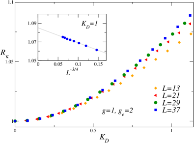
Figure 3: Plot of the ratio $R_{\kappa}$, defined in Eq. (22), versus $K_{D}=\kappa L^{1/2}$, for $g=1$ and $g_{e}=2$. Data appear to converge with increasing $L$ onto a single curve, supporting the scaling behavior, Eq. (20). In the inset we show data for $K_{D}=1$: scaling corrections apparently behave as $L^{-3/4}$ (the straight line is only meant to guide the eye), as predicted by RG arguments.

IV.1.2 Ising-like transition lines for small $\kappa$

As already anticipated, we may also predict the behavior of the Ising transition line $g_{c}(\kappa)$, starting at the critical point $g_{c}=g_{\cal I}$ for $\kappa=0$. Transitions occur on the line $u_{r}=0$. Eq. (19) implies

$$g_{c}(g_{e},\kappa)-g_{c}(g_{e},\kappa=0)=g_{c}(g_{e},\kappa)-g_{\cal I}\approx b(g_{e})\,\kappa^{2}\,,$$ (23)

where $b$ depends only on $g_{e}$. The behavior (23) holds for sufficiently small values of $\kappa$, when higher-order $O(\kappa^{4})$ terms in the expansion (19) can be neglected.

In App. B we determine $b(g_{e})$ for large values of $g_{e}$, obtaining

$$b(g_{e})\approx{3\over 2g_{e}^{2}}\qquad{\rm for}\;g_{e}\to\infty\,.$$ (24)

The vanishing of $b(g_{e})$ far large $g_{e}$ follows from the more general result $g_{c}(g_{e},\kappa)=g_{\cal I}$ for any $\kappa$ in the limit $g_{e}\to\infty$. Indeed, in this limit the ground state of the global system is an eigenvector of $\tau_{\bm{x}}^{(3)}$ with eigenvalue 1 for all lattice points $\bm{x}$. The global ground state is therefore factorized, i.e., $|\Psi_{0}\rangle=|\phi_{0}\rangle_{\cal E}\otimes|\psi_{0}\rangle_{\cal S}$, where $|\phi_{0}\rangle_{\cal E}=\Pi_{\bm{x}}|+\rangle_{\bm{x}}$, $|+\rangle_{\bm{x}}$ is the $+1$ eigenvector of $\tau_{\bm{x}}^{(3)}$, and $|\psi_{0}\rangle_{\cal S}$ is defined on $\cal S$ only. Since the matrix element of $H_{\cal SE}$ on this factorized state vanishes, $|\psi_{0}\rangle_{\cal S}$ is the ground state of an isolated single Ising chain, that has critical point for $g=g_{\cal I}$, independently of $\kappa$.

We now consider the opposite limit, $r_{e}\equiv g_{e}-g_{\cal I}\to 0$. In this case the coefficient $b(g_{e})$ is expected to diverge as $b(g_{e})\sim r_{e}^{-\zeta}$. with $\zeta>0$. The exponent $\zeta$ will be determined in Sec. IV.2.2, by matching Eq. (23) with the asymptotic multicritical behavior arising when also the environment is critical. This allows us to obtain the exponent $\zeta$ in terms of the Ising critical exponents. We find $\zeta=2(2-\eta)\nu-1>0$ and, in particular, $\zeta=5/2$ for one-dimensional stacked Ising chains. The divergence of $b(g_{e})$ for $r_{e}\to 0$, indicates that a different regime emerges when the environment ${\cal E}$ is critical, as it will be discussed in Sec. IV.2.

The prediction (23) is nicely confirmed by the numerical results. In Fig. 4 we report the critical points $g_{c}(\kappa)$ for $g_{e}=2$ and $g_{e}=4$ and a few values of $\kappa$. The critical points were identified by looking at the crossing points of the ratio $R_{\kappa}$ defined in Eq. (22), for systems with OBC and lattice sizes up to $L\approx 20$.

Finally, we consider the susceptibility $\chi$ as a function of $R_{\xi}=\xi/L$. In Fig. 5 we report $\chi/L^{1-\eta}$ computed varying $g$ around the critical point $g_{c}(\kappa)$ for several different values of $L$ and $\kappa$, and for two values of $g_{e}$. According to the RG theory, data should scale according to Eq. (15). The results reported in Fig. 5 show an excellent scaling, provided we use the Ising exponent $\eta=1/4$. They confirm that all transitions for $\kappa>0$ belong to the 2D Ising universality class. Note, moreover, that data corresponding to different values of $g_{e}$ and $\kappa$ appear to approximately collapse onto the same curve. This implies that the nonuniversal constant $a_{\chi}$ is Eq. (15) depends very weakly on the system parameters.

To conclude, let us finally note that the coupling $\kappa$ also significantly affects the properties of the environment $\cal E$: For $\kappa\not=0$ the environment becomes critical when $\cal S$ is driven to criticality. Thus, only for $g>g_{c}(\kappa)$ is the environment still disordered. For $g=g_{c}(\kappa)$, $\cal E$ is critical, while, for $g<g_{c}(\kappa)$ the environment is fully ordered. These features will be discussed and explained on general grounds in Sec. V.

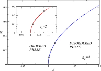
Figure 4: The $g$-$\kappa$ phase diagram when the environment is disordered in the absence of coupling, i.e., for $g_{e}>g_{\cal I}=1$. We report the estimates of the critical points for $g_{e}=4$ and some values of $\kappa$. In the inset we report analogous data for $g_{e}=2$. The uncertainty on the estimates is smaller than, or at the most of the order of, the size of the symbols. The critical lines are obtained by fitting the data for the smallest values of $\kappa$ (those along the full lines) to $g_{c}(\kappa)=1+b\,\kappa^{2}$, obtaining $b\approx 0.14$ for $g_{e}=4$, and $b\approx 1.29$ gor $g_{e}=2$. These results fully support the RG prediction, Eq. (23). The coefficient $b$ rapidly increases when $g_{e}$ approaches the critical value $g_{\cal I}=1$, consistently with the asymptotic behavior $b(g_{e})\sim(g_{e}-1)^{-5/2}$, see Eq. (42).

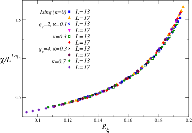
Figure 5: Plot of $\chi/L^{1-\eta}$ versus $R_{\xi}$. For each $L$, $\kappa$, and $g_{e}$, data are obtained by varying $g$ around the critical point $g_{c}(\kappa)$. The Ising exponent $\eta=1/4$ is used.

IV.2 Critical environment

We now discuss how the coupling with a critical environment ${\cal E}$ affects the critical behavior of the subsystem ${\cal S}$. Therefore, we assume that ${\cal E}$ is close to criticality for $\kappa=0$, i.e., $g_{e}\approx g_{\cal I}$. As we shall see, the effect of a weak coupling between ${\cal S}$ and ${\cal E}$ is substantially different from that occurring when ${\cal S}$ is coupled with a disordered environment.

IV.2.1 FSS at the multicritical point for $\kappa=0$

As we shall show below, if the environment ${\cal E}$ is critical, the interaction $H_{\cal SE}$ gives rise to a relevant perturbation of the critical behavior of the subsystem $\cal S$. In this case there are three relevant perturbations at the uncoupled critical point $(g=g_{\cal I},g_{e}=g_{\cal I},\kappa=0)$. Two of them are those that drive criticality in the two isolated subsystems. The coupling $\kappa$ gives rise to an additional independent relevant RG perturbation.

The uncoupled critical point is multicritical. To describe the multicritical behavior close to it FN-74 ; NKF-74 ; PV-02 ; CPV-03 ; BPV-22 , we introduce three independent scaling fields,

$$u_{r}\sim r\equiv g-g_{\cal I},\quad u_{er}\sim r_{e}\equiv g_{e}-g_{\cal I},\quad u_{\kappa}\sim\kappa.$$ (25)

Because of the equivalence of the environment and the system, $u_{r}$ and $u_{er}$ have the same RG dimension $y_{r}$. The scaling field $u_{\kappa}$ has RG dimension $y_{\kappa}$. All scaling fields are relevant: $y_{r}$ and $y_{\kappa}$ are both positive, see below. Then, in the zero-temperature and FSS limit, the singular part of the free-energy density is expected to scale as Wegner-76 ; PV-02 ; CPV-03 ; CPV-14 ; RV-21

$$F_{\rm sing}(g,g_{e},\kappa,L)\approx L^{-(d+z)}{\cal F}(W_{s},W_{es},K_{s})\,,$$ (26)

$$W_{s}=u_{r}L^{y_{r}}\,,\quad W_{es}=u_{er}L^{y_{r}}\,,\quad K_{s}=u_{\kappa}L^{y_{\kappa}}\,.\qquad$$ (27)

The scaling fields $u_{r}$, $u_{er}$, and $u_{\kappa}$ are analytic functions of the Hamiltonian parameters $g$, $g_{e}$, and $\kappa$. Close to the multicritical point they can be expanded as

$$u_{r}=r+b_{\kappa}\kappa^{2}+b_{r}r^{2}+b_{er}rr_{e}\ldots\,,$$ (28)

$$u_{er}=r_{e}+c_{\kappa}\kappa^{2}+c_{r}r_{e}^{2}+c_{er}rr_{e}\ldots\,,$$ (29)

$$u_{\kappa}=\kappa+d_{r}r\kappa+d_{er}r_{e}\kappa\ldots\,.$$ (30)

The scaling fields $u_{r}$ and $u_{er}$ are expected to be even under the symmetry $\kappa\to-\kappa$ (therefore they can only depend on $\kappa^{2}$), while $u_{\kappa}$ should be odd. Since we are interested in the asymptotic FSS, we may equivalently consider the simpler linear scaling variables

$$W=rL^{y_{r}}\,,\qquad W_{e}=r_{e}L^{y_{r}}\,,\qquad K=\kappa L^{y_{\kappa}}\,.$$ (31)

This substitution is equivalent to neglecting some (typically next-to-leading CPV-14 , see also below) scaling corrections.

Close to the multicritical point, the effects of a small coupling $\kappa$ are controlled by its RG dimension $y_{\kappa}$. To compute it, we note that the interaction term can be rewritten in the field-theory framework as RLXP-20 ; LLM-98

$$\int d^{D}x\;\kappa\;\phi_{s}({\bm{x}})\phi_{e}({\bm{x}})\,,\qquad D=d+z\,,$$ (32)

where $\phi_{s}$ and $\phi_{e}$ are the order-parameter fields for the two critical systems ${\cal S}$ and ${\cal E}$. Then, we straightforwardly obtain

$$y_{\kappa}=d+z-2y_{\phi}=2-\eta\,,$$ (33)

where $y_{\phi}$ is the RG dimension of the order parameter at the $(d+1)$-dimensional Ising fixed point. These relations give $y_{\kappa}=7/4$ for $d=1$, $y_{\kappa}=1.963702(2)$ for $d=2$, and $y_{\kappa}=2$ for $d=3$, confirming that the coupling $\kappa$ gives rise to a relevant perturbation, as anticipated above.

On the basis of the above RG analysis, we expect any RG invariant quantity $R$ defined on the subsystem ${\cal S}$, such as $R_{\xi}=\xi/L$ or the decoherence factor $Q$, to behave as

$$R(g,g_{e},\kappa,L)\approx{\cal R}(W,W_{e},K)\,,$$ (34)

where ${\cal R}$ is a universal scaling function of its arguments. In particular, if we set $r=r_{e}=0$, therefore moving along the line $g=g_{e}=g_{\cal I}$, Eq. (34) predicts

$$R(g=g_{\cal I},g_{e}=g_{\cal I},\kappa,L)\approx{\cal R}_{0}(K)\,.$$ (35)

Differentiating twice Eq. (34) with respect to $\kappa$, and then setting $\kappa=0$, we obtain the leading FSS behavior of the decoherence susceptibility $\chi_{Q}$ defined in Eq. (10):

$$\chi_{Q}(g,g_{e},L)\approx L^{2y_{\kappa}}{\cal C}(W,W_{e})\,.$$ (36)

Again this demonstrates that the coherence properties of the quantum critical behavior of ${\cal S}$ are very sensitive to the coupling with the environment ${\cal E}$. We may compare the power-law behavior $\chi_{Q}(g,g_{e},L)\approx L^{2y_{\kappa}}$ with that obtained when ${\cal E}$ is disordered for $\kappa=0$, i.e., $\chi_{Q}\sim L^{y_{r}}$, cf. Eq. (21). The exponent $2y_{\kappa}$ is significantly larger than $y_{r}$ in any dimension (indeed $y_{r}=1$ and $2y_{\kappa}=7/2$ in $d=1$; $y_{r}\approx 1.587$ and $2y_{\kappa}\approx 3.928$ in $d=2$; $y_{r}=2$ and $y_{\kappa}=4$ in $d=3$) and thus, not surprisingly, the decoherence rate for a critical environment is much larger than that for a disordered environment.

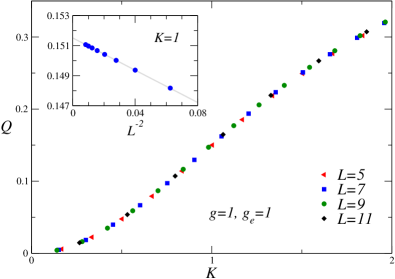
Figure 6: The decoherence function $Q$ for $g=g_{e}=1$ (correspondingly, $r=r_{e}=0$). The data show an excellent FSS when plotted versus $K=\kappa L^{7/4}$, confirming the RG analysis. The inset shows the data at fixed $K=1$: size corrections apparently decay as $L^{-2}$, as predicted by the RG arguments (the line is only drawn to guide the eye).

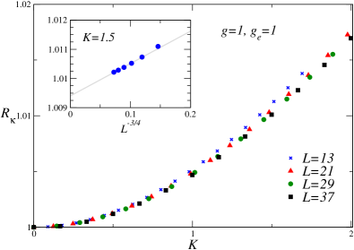
Figure 7: Scaling behavior of the ratio $R_{\kappa}$, defined in Eq. (22), for $g=g_{e}=1$ (corresponding to $r=r_{e}=0$). The data show an asymptotic FSS when plotted versus $K=\kappa L^{7/4}$, confirming the RG analysis. The inset shows the data at fixed $K=1.5$: size corrections decay as $L^{-3/4}$, as expected from the RG arguments (the line is only drawn to guide the eye).

To verify the previous scaling predictions, we have considered two coupled chains at criticality, i.e., for $g=g_{e}=g_{\cal I}=1$. We recall that $y_{r}=1$ and $y_{\kappa}=7/4$ for one-dimensional systems. Figs. 6 and 7 show the behavior of the decoherence factor $Q$ (we use PBC) and of the ratio $R_{\kappa}$ defined in Eq. (22) (we use OBC), respectively. The results for both $Q$ and $R_{\kappa}$ nicely support the scaling behavior, Eq. (35). In particular, the observed scaling behavior of $Q$ implies the divergence of the decoherence susceptibility, $\chi_{Q}\sim L^{2y_{\kappa}}$.

Scaling corrections are expected to be similar to those arising in the case of an isolated critical Ising chain, see also Sec. IV.1. For one-dimensional quantum Ising systems, the leading scaling correction for the ratio $R_{\xi}=\xi/L$ is expected to be due to the analytic background CPV-14 : it should decay as $L^{-3/4}$ for both PBC and OBC. The scaling corrections associated with $Q$ are expected to decay faster, as $L^{-2}$ in the absence of boundaries (for instance, for PBC), and as $L^{-1}$ for systems with boundaries (in the OBC case). The insets of Figs. 6 and 7 show that scaling corrections behave as predicted by the RG arguments.

We remark that similar multicritical behaviors should also emerge when the two subsystems ${\cal S}$ and ${\cal E}$ are different. The multicritical fixed point is given by the two decoupled fixed points associated with the critical behaviors of ${\cal S}$ and ${\cal E}$ in the absence of any coupling. The RG dimension of the parameter $\kappa$ that parametrizes the coupling of the two subsystems can be computed again using Eq. (32), where $\phi_{s}$ and $\phi_{e}$ represent the operators defined in ${\cal S}$ and ${\cal E}$ entering the interaction Hamiltonian $H_{\cal SE}$.

IV.2.2 Ising transition lines for small $\kappa$

So far we have considered the behavior around the multicritical point. In the parameter space $(g,g_{e},\kappa)$, the multicritical point $(g=g_{\cal I},g_{e}=g_{\cal I},\kappa=0)$ belongs to a two-dimensional surface of critical transitions that lies, for $\kappa\not=0$, in the region $g>g_{\cal I}$, $g_{e}>g_{\cal I}$. Such transitions are related to the spontaneous breaking of the residual ${\mathbb{Z}}_{2}$ symmetry of the global system when $\kappa\neq 0$. Therefore, they are expected to belong to the $(d+1)$-dimensional Ising universality class. A more general discussion will be presented in Sec. V. Here, we wish to discuss the shape of the critical surface close to the multicritical point.

To make the discussion simple, let us consider a plane in the parameter space such that the ratio $s\equiv r_{e}/r$ is constant, and such that it intersects the transition surface along a line. The scaling behavior (26) of the free energy also determines the behavior of the transition line close to the multicritical point, see, e.g., Refs. FN-74 ; NKF-74 ; CPV-03 . As $r_{e}/r=W_{e}/W$ is kept constant, we can neglect the scaling field $W_{e}$, and we can rewrite the singular free-energy density as

$$F\approx\xi_{r}^{-(d+z)}\widetilde{\cal F}(X,Y)\,,$$ (37)

$$X=\xi_{r}/L\,,\quad\xi_{r}\sim r^{-1/y_{r}}\,,\quad Y=r^{-y_{\kappa}/y_{r}}\kappa\,,\qquad$$ (38)

where $\xi_{r}$ plays the role of a critical length scale. In the large-$L$ limit, i.e., for $X\to 0$, we may write

$$F\approx\xi_{r}^{-(d+z)}{\cal F}_{\infty}(Y)\,.$$ (39)

Consistency of the phase diagram with Eq. (39) requires that, for $\kappa\to 0$, the critical line $g_{c}(s,\kappa)$ is tangent to the line corresponding to a fixed finite value of the scaling variable $Y$. Therefore, for small values of $\kappa$, the above scaling arguments predict that

$$g_{c}(s,\kappa)-g_{\cal I}\approx w(s)\,\kappa^{\varepsilon}\,,\quad\varepsilon={y_{r}\over y_{\kappa}}\leq 1\,,\quad s={r_{e}\over r}\,,$$ (40)

where the coefficient $w(s)$ depends on the ratio $s=r_{e}/r$. Substituting the known values of $y_{r}$ and $y_{\kappa}$, we find $\varepsilon=4/7\approx 0.5714$ for $d=1$, $\varepsilon\approx 0.8084$ for $d=2$, and $\varepsilon=1$ for $d=3$ [in $d=3$, there are probably additional multiplicative logarithms in Eq. (40)]. The small-$\kappa$ behavior (40) significantly differs from that holding for a disordered environment, see Eq. (23).

As discussed in Sec. IV.1.2, $g_{c}(s,\kappa)-g_{\cal I}=O(\kappa^{2})$ for finite $r_{e}\equiv g_{e}-g_{\cal I}>0$, thus the coefficient $w(s)$ of the power $\kappa^{\varepsilon}$ (where $\varepsilon<2$) must vanish for $s\to\infty$. The consistency of the scaling equation (40) with Eq. (23) in the limit $g_{e}\to g_{\cal I}$ allows us to predict the limiting behavior of $b(g_{e})$ appearing in Eq. (23) for $g_{e}\to g_{\cal I}$ and of $w(s)$ for $s\to\infty$. Indeed, for small values of $\kappa$, Eq. (23) can be rewritten as

$$g_{c}(g_{e},\kappa)-g_{\cal I}=\left\{{b(g_{e})\,[g_{c}(g_{e},\kappa)-g_{\cal I}]^{2/\varepsilon-1}}\right\}^{\varepsilon/2}\kappa^{\varepsilon}\,.$$ (41)

We require this relation to be consistent with the scaling behavior Eq. (40) for $r_{e}\equiv g_{e}-g_{\cal I}\to 0$. This implies

$$b(g_{e})\sim r_{e}^{-\zeta}\,,\quad\zeta={2\over\varepsilon}-1=2(2-\eta)\nu-1\,.$$ (42)

Explicitly, $\zeta=5/2,1.47,1$ for $d=1,2,3$, respectively. Eq. (41) also predicts the behavior of $w(s)$ when $w(s)\to 0$, i.e., for large values of $s$. We find

$$w(s)\sim s^{-\rho}\,,\qquad\rho=1-\varepsilon/2>0\,.$$ (43)

For $d=1,2,3$ we have $\rho=5/7$, $\rho\approx 0.596$, $\rho=1/2$, respectively.

We would like to stress that the above RG arguments determine the behavior of the critical lines starting from the multicritical point, provided it exists. However, they do not ensure the existence of such line for any value of $s$. Indeed, the mean-field calculations reported in App. A, suggest that the critical lines exist only for $s>0$. Our numerical results, see below, confirm this prediction.

As we shall discuss in Sec. V, if the $\cal S$ correlations are critical, also correlations defined on $\cal E$ are critical. Using the symmetry of the system under the exchange of $\cal S$ and $\cal E$, see Sec. II, we can straightforwardly obtain a relation on the location of the (common) critical points. The coefficient $w(s)$ in Eq. (40) must satisfy the relation

$$w(s^{-1})=s\,w(s)\,.$$ (44)

This relation combined with Eq. (43) implies that $w(s)$ diverges as $s\to 0$, as

$$w(s)\sim s^{-\varepsilon/2}\quad{\rm for}\;s\to 0\,.$$ (45)

The divergence of $w(s)$ for $s\to 0$ suggests that the transition line starting from the multicritical point disappears for $s=0$, i.e. when $g_{e}=g_{\cal I}$, confirming the mean-field analysis. This is also supported by the numerical results for the stacked Ising chains, see below.

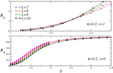
Figure 8: Plot of the ratio $R_{\Delta}$ defined in Eq. (46) for $\kappa=0.2$. Top: results for $s=1$; bottom: results for $s=0$. Results for $s=1$ show a clear crossing point for $g\approx 1.31$, indicating the presence of a transition. For $s=0$ the ratio $R_{\Delta}$ is always smaller than 1 and does not show any crossing, indicating that no transition occurs.

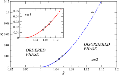
Figure 9: Estimates of the critical points $g_{c}(\kappa)$ for some values of $\kappa$ for $s\equiv r_{e}/r=2$ and $s=1$ (inset). The behavior for small $\kappa$ is in agreement with the scaling prediction, Eq. (40). The full lines are obtained by fitting the estimates of $g_{c}(\kappa)$ for small values of $\kappa$ ($\kappa\lesssim 0.03$) to $g_{c}(\kappa)=1+w\,\kappa^{\varepsilon}$ with $\varepsilon=4/7$. We obtain $w\approx 0.53$ for $s=2$ and $w\approx 0.76$ for $s=1$. Note that $w$ decreases with increasing $s$, as expected on the basis of the asymptotic behavior (43).

To check these predictions, we again consider the stacked Ising chains and numerically determine $g_{c}(s,\kappa)$ for a few small values of $\kappa$. For this purpose, we determine the energy gap $\Delta$, i.e., the difference of the energies of the two lowest states of the global system, focusing on the ratio

$$R_{\Delta}(s,r,\kappa,L)={\Delta(s,r,\kappa,L)\over\Delta_{\cal I}(L)}\,,$$ (46)

where $\Delta_{\cal I}\sim L^{-1}$ is the gap of the single critical Ising chain. We consider systems with PBC and compute the gap using exact-diagonalization techniques. Since the transition line is expected to belong to the Ising universality class—therefore $z=1$—the ratio $R_{\Delta}$ is expected to vanish for $g<g_{c}(s,\kappa)$ and to diverge for $g>g_{c}(s,\kappa)$. In particular, close to the transition point, at fixed $\kappa$, it should scale as

$$R_{\Delta}(s,g,\kappa)\approx{\cal R}_{\Delta}(UL^{y_{r}})\,,\qquad U=g-g_{c}(s,\kappa)\,,$$ (47)

where ${\cal R}_{\Delta}(x)$ is a universal scaling function, apart from a multiplicative factor and a rescaling of its argument. The RG invariant ratio $R_{\xi}$ should scale analogously, i.e., we should have $R_{\xi}(s,g,\kappa)\approx{\cal R}_{\xi}(UL^{y_{r}})$ where ${\cal R}_{\xi}$ is universal apart from a rescaling of its argument. Therefore, the transition point $g_{c}(s,\kappa)$ can be determined by looking for the crossing point of data sets for different sizes $L$.

In Fig. 8 we show $R_{\Delta}$ at fixed $\kappa=0.2$ for two values of $s$, that is, $s=1$ and $s=0$. The data for $s=1$ show a crossing point indicating the existence of a transition point, while those for $s=0$ are always smaller than 1 and do not show any crossing, indicating that there is no transition for finite $\kappa$ and $s=0$ (i.e., $g_{e}=1$). Note that for $s=0$ the ratio $R_{\Delta}$ is expected to approach 1 for $g\to\infty$. Indeed, when $g\to\infty$, the ground state becomes an eigenvector of all $\sigma_{\bm{x}}^{(3)}$ operators. It is immediate to verify that this implies an effective decoupling of the critical environment ${\cal E}$ (the argument is the same as the one used to discuss the limit $g_{e}\to\infty$ in Sec. IV.1.2). The gap of the global system therefore converges to the gap $\Delta_{\cal I}$ of the isolated environment.

In Fig. 9 we show some results for the critical lines starting from the multicritical point, for some values of $s>0$. We mention that some results for identical stacked critical Ising chains, i.e. for $g=g_{e}$, thus corresponding to $s=1$, were already reported in Ref. RLXP-20 . Our results and those reported in Ref. RLXP-20 nicely confirm the scaling prediction (40). Moreover, our numerical results do not provide evidence of transitions for $s\leq 0$ (including also the marginal case $s=0$, as shown above), supporting the absence of transition lines when one of the coupling $g$ or $g_{e}$ is below the Ising-chain transition point $g_{\cal I}$, as predicted by the mean-field analysis reported in App. A.

We also mention that consistent results (not shown) have also been obtained by analyzing the FSS behavior of $R_{\xi}$ or of the ratio $R_{\kappa}$ defined in Eq. (22). The DMRG results for systems with OBC show a slower convergence to the asymptotic large-$L$ behavior, therefore leading to less precise estimates. This can be explained by the different behavior of the size corrections for the two observables. If PBC are used, $R_{\Delta}$ approaches the asymptotic value with corrections that decay as $L^{-2}$ CPV-14 . On the other hand, for $R_{\xi}$ (for both PBC and OBC), size corrections decay slower, as $L^{-3/4}$.

IV.3 Ordered environment

Finally, we discuss the behavior of ${\cal S}$ when the environment ${\cal E}$ is ordered and characterized by a nonzero magnetization in the thermodynamic limit. In Ising systems, this corresponds to choosing $g_{e}<g_{\cal I}$ and appropriate boundary conditions (see below). We argue that, as in the case of a critical environment, the interaction term $H_{\cal SE}$ is a relevant perturbation. However, its RG dimension $\bar{y}_{\kappa}$ differs from that controlling the behavior in a critical environment, since $\bar{y}_{\kappa}>y_{\kappa}$. Moreover, no transition lines appear at finite $\kappa$; therefore for $g_{e}<g_{\cal I}$, the critical point at $g=g_{\cal I}$ and $\kappa=0$ is isolated.

For a magnetized environment, the order parameter of the subsystem ${\cal E}$ is not critical, as the ground state of ${\cal E}$ is the superposition of magnetized states with magnetization $\pm m_{0}$ (the superposition must be such that the global magnetization vanishes because of the global ${\mathbb{Z}}_{2}$ symmetry of the global Hamiltonian). Therefore, in the perturbation (32) we can replace $\phi_{e}({\bm{x}})$ with an average magnetization, which is a constant under RG transformations. The RG perturbation (32) reduces to

$$\int d^{D}x\;\kappa\;\phi_{s}({\bm{x}})\,,$$ (48)

which leads to

$$\bar{y}_{\kappa}=d+z-y_{\phi}=y_{h}\,,$$ (49)

where $y_{h}$ is the RG dimension of the leading symmetry-breaking perturbation at the Ising fixed point, associated with a longitudinal field $h$, see Sec. II. Therefore, $y_{h}=15/8$ for $d=1$, $y_{h}\approx 2.482$ for $d=2$, and $y_{h}=3$ for $d=3$. These results imply that the singular part of the free-energy density in the zero-temperature and FSS limit scales as

$$F_{\rm sing}(r,\kappa,L)\approx L^{-(d+z)}{\cal F}(W,K_{O})\,,$$ (50)

$$W\approx rL^{y_{r}}\,,\qquad K_{O}\approx\kappa L^{y_{h}}\,,$$ (51)

where $r=g-g_{\cal I}$ and we used linear scaling fields. The specific value of the coupling $g_{e}<g_{\cal I}$ does not play any role. It only changes the values of the nonuniversal constants and of the analytic backgrounds.

The scaling behavior for any observable can be straightforwardly obtained from those reported for the critical environment. It is enough to replace the scaling variable $K$ with $K_{O}$ and $y_{\kappa}$ with $y_{h}$, in Eqs. (34), (35), and (36). In particular, the decoherence susceptibility behaves as

$$\chi_{Q}\sim L^{2y_{h}}\,.$$ (52)

Therefore, since $y_{h}>y_{\kappa}$ for any $d$ (indeed $y_{h}-y_{\kappa}=y_{\phi}>0$), the sensitivity of the coherence properties when ${\cal E}$ is in the ordered phase is even larger than the one arising from a critical environment ${\cal E}$, where $\chi_{Q}\sim L^{2y_{\kappa}}$.

The leading scaling corrections for $R_{\xi}$ and $Q$ are analogous to those found for a critical environment. For example, for one-dimensional systems with PBC, we expect $O(L^{-2})$ corrections for $Q$ and $O(L^{-3/4})$ corrections for $R_{\xi}$.

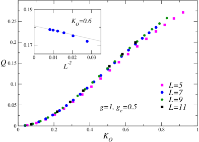
Figure 10: Decoherence function $Q$ versus $K_{O}=\kappa L^{y_{h}}$, for $g=g_{\cal I}=1$ and $g_{e}=0.5$ (ordered environment). In the inset, we show data for $K_{O}=0.6$: size corrections decay as $L^{-2}$ in agreement with RG arguments (the line is drawn to guide the eye).

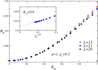
Figure 11: Ratio $R_{\kappa}$, defined in Eq. (22), versus $K_{O}=\kappa L^{y_{h}}$, for $g=g_{\cal I}=1$ and $g_{e}=0.5$ (ordered environment). In the inset, we show data at fixed $K_{O}=0.8$: size corrections decay as $L^{-3/4}$ in agreement with RG arguments (the line is drawn to guide the eye).

The FSS predictions are confirmed by the results of numerical computations for coupled quantum Ising chains. We fixed $g=g_{\cal I}=1$ and considered two values of $g_{e}$, $g_{e}=0.2$ and $g_{e}=0.5$. Results for the decoherence factor $Q$ for a system with PBC and for $R_{\kappa}$ defined in Eq. (22) for a system with OBC are shown in Figs. 10 and 11, respectively. The results nicely support the scaling behavior (50).

Since the parameter $\kappa$ effectively behaves as an external longitudinal field when $g_{e}<g_{\cal I}$, we do not expect any transition for finite values of $\kappa$, as in the standard quantum Ising model in the presence of an external longitudinal field $h$. This is confirmed by numerical results.

We finally stress that the derivation of the above scaling behaviors assumes that the environment ${\cal E}$ is subject to neutral boundary conditions, i.e., to boundary conditions that do not favor any ordered phase, such as PBC and OBC. Only with these boundary conditions is the ground state a superposition of magnetized states CNPV-14 . Some important changes may occur when different boundary conditions are considered, for example, fixed boundary conditions that favor one of the broken phases, or antiperiodic boundary conditions. Indeed, the FSS of systems at quantum first-order transitions drastically depends on the nature of the boundary conditions, see, e.g., Refs. CNPV-14 ; CPV-15 ; PRV-18-fo ; RV-21 .

V General phase diagram

In Sec. IV, we discussed the behavior of the subsystem ${\cal S}$ in the weak-coupling regime $\kappa\ll 1$. We wish to discuss now the behavior for finite values of $\kappa$. We recall that the phase diagram of the global system must be symmetric with respect to a change of the sign of $\kappa$ at fixed $g$ and $g_{e}$. Moreover, at fixed $\kappa$, it must be symmetric with respect to interchanging $g$ and $g_{e}$, due to the fact that the two subsystems ${\cal S}$ and ${\cal E}$ are identical apart from the transverse couplings $g$ and $g_{e}$.

A mean-field analysis is presented in App. A, which shows that, also for finite $\kappa$, the environment parameter $g_{e}$ plays an important role. The main features of the mean-field analysis are substantially confirmed by the numerical results that we have obtained for the stacked Ising chains.

If the environment is ordered in the absence of coupling, i.e., for $g_{e}<g_{\cal I}$, no transition occurs for any value of $\kappa$. The coupling with the environment drives the system ${\cal S}$ in the ordered phase, independently of the value of $g$. A critical behavior is only observed for $\kappa=0$ and $g=g_{\cal I}$, as discussed in Sec. IV.3. A different behavior is observed for $g_{e}>g_{\cal I}$, i.e., when the environment is disordered in the absence of coupling. In this case, by tuning $g$ to a critical value $g_{c}(\kappa,g_{e})>g_{\cal I}$, a critical line appears, which should be associated with the breaking of the global ${\mathbb{Z}}_{2}$ symmetry, cf. Eq. (II). This is shown in Fig. 4.

It is interesting to observe that, at the critical point, both correlations defined on $\cal S$ and on $\cal E$ are critical. This is a specific feature of the interaction we consider, or, more precisely, of the invariance properties of the interaction term $H_{\cal SE}$. In general, at fixed $g$ and $g_{e}$, one may expect different types of transitions: a transition at $\kappa=\kappa_{\cal S}(g,g_{e})$, where $\cal S$ correlations are critical, and a transition at $\kappa=\kappa_{\cal E}(g,g_{e})$, where $\cal E$ correlations are critical. Note that we are making no assumption of the existence of the transitions: at fixed $g$ and $g_{e}$, there may be no transition, one transition, or both of them. The symmetry of the system under the exchange of $\cal S$ and $\cal E$ implies $\kappa_{\cal S}(g,g_{e})=\kappa_{\cal E}(g_{e},g)$, but not the equality of the two functions. The relation $\kappa_{\cal S}(g,g_{e})=\kappa_{\cal E}(g,g_{e})$ follows instead from the analysis of the symmetry breaking pattern at the transition. Indeed, in our model the symmetry involves transformations on both systems, see Eq. (II). Thus, we expect both systems to be magnetized on the ordered side of the transition, which, in turn, implies that they become critical simultaneously. This prediction has been explicitly verified in Sec. IV.3. Note that the equality of the two transition functions does not necessarily hold, if the interaction term does not break the symmetry under independent longitudinal spin reflections. This would be the case of subsystems coupled by using the transverse spin operators, for instance, by the Hamiltonian interaction (7). In this case, for $g\not=g_{e}$, one might observe two different transitions.

Since the $\cal E$ and the $\cal S$ subsystems become simultaneously critical, for $g<g_{c}(\kappa)$, both $\cal S$ and ${\cal E}$ should be ordered, as verified in Sec. IV.3. For $g>g_{c}(\kappa)$ instead, both subsystems should be disordered. Since the global ${\mathbb{Z}}_{2}$ symmetry is broken at $g_{c}(\kappa)$, the transition should belong to the Ising universality class and $g-g_{c}(\kappa)$ should represent the scaling field associated with the leading even perturbation, analogous to $r=g-g_{\cal I}$ for standard Ising systems. This is confirmed by the scaling plots reported in Fig. 5.

The intermediate situation where $g_{e}\approx g_{\cal I}$ gives rise to a multicritical behavior, as discussed in Sec. IV.2. In agreement with the mean-field analysis, the numerical results confirm that there are no transitions at finite $\kappa$ when $g_{e}\leq g_{\cal I}$. In the opposite case $g_{e}>g_{\cal I}$, the transition lines are present. Their behavior for $\kappa\to 0$ and $g_{e}\to g_{\cal I}$, is consistent with the expected multicritical scaling, see Fig. 9.

Finally, let us consider the behavior in the limit $\kappa\to\infty$. A general discussion is reported in App. B. We show that the system is fully ordered for $\kappa\to\infty$ at fixed $g$ and $g_{e}$. For finite, large values of $\kappa$, a transition always occurs for large values of $g$. More precisely, $g_{c}(\kappa)\approx a\kappa$ for $\kappa\to\infty$, where $a$ is a constant dependent on $g_{e}$, see App. B.

VI Out-of-equilibrium dynamic scaling behavior

The recent progress achieved by quantum simulators in controlling the dynamics of an increasing number of qubits has called for theoretical investigations of the coherent time evolution of quantum correlations in composite systems, of the decoherence of one subsystem due to the interaction with the remainder, and of the energy exchanges between finite-size subsystems (see, e.g., Refs. RV-21 ; Dziarmaga-10 ; PSSV-11 ; GAN-14 ; NC-book ). A deeper understanding of the decoherence and entanglement dynamics is of fundamental importance, both for quantum-information purposes and for the improvement of energy conversion in complex networks NC-book ; LCCLCN-13 . Moreover, the study of the energy storage and exchange among the different components of a quantum system is relevant for quantum-thermodynamical purposes GHRRS-16 ; VA-16 , as well as for the efficiency optimization of recently developed quantum batteries CPV-18 .

The study of the phase diagram and of the equilibrium scaling properties reported in the previous sections allows one to describe the adiabatic slow dynamics of finite-size systems (we recall that finite-size many-body systems are generally gapped). In this section we extend the analysis to out-of-equilibrium dynamic protocols. In particular, we wish to determine the dynamic scaling behaviors induced by a time-dependent coupling between the subsystems ${\cal S}$ and ${\cal E}$.

We consider here the following quenching protocol. Initially, the systems ${\cal S}$ and ${\cal E}$ are decoupled, i.e., $\kappa=0$, and are in their ground states $|\Psi^{({\cal S})}_{0}\rangle$ and $|\Psi^{({\cal E})}_{0}\rangle$, so that the initial many-body state $|\Psi_{0}\rangle$ is given by

$$|\Psi_{0}\rangle=|\Psi^{({\cal S})}_{0}\rangle\otimes|\Psi^{({\cal E})}_{0}\rangle\,.$$ (53)

Then, at $t=0$, the system is suddenly driven out of equilibrium by quenching the parameter $\kappa$ to a finite value, i.e., $\kappa$ varies instantaneously from zero to a finite value $\kappa>0$. The initial state $|\Psi_{0}\rangle$ is no longer a Hamiltonian eigenstate and it evolves according to the Schrödinger equation,

$$|\Psi(t)\rangle=e^{-iHt}|\Psi_{0}\rangle\,,$$ (54)

where $H$ is the total Hamiltonian (1).

One can easily check that a sudden quench from $\kappa=0$ to any $\kappa>0$ entails a vanishing average quantum work

$$W = \langle\Psi(t)|H_{\cal S}(g)+H_{\cal E}(g_{e})+H_{\cal SE}(\kappa)|\Psi(t)\rangle$$ (55)

$$-\langle\Psi_{0}|H_{\cal S}(g)+H_{\cal E}(g_{e})|\Psi_{0}\rangle\,.$$

Indeed, since we are interested in a sudden quench at $t=0$, and the average energy is conserved for $t>0$, we can compute the average work replacing $|\Psi(t)\rangle$ with $|\Psi_{0}\rangle$, thus obtaining

$$W = \langle\Psi_{0}|H_{\cal SE}(\kappa)|\Psi_{0}\rangle$$

$$= -\kappa\sum_{\bm{x}}\langle\Psi^{({\cal S})}_{0}|\sigma_{\bm{x}}^{(1)}|\Psi^{({\cal S})}_{0}\rangle\langle\Psi^{({\cal E})}_{0}|\tau_{\bm{x}}^{(1)}|\Psi^{({\cal E})}_{0}\rangle=0\,,$$

where we used the fact that $\langle\Psi^{({\cal S})}_{0}|\sigma_{\bm{x}}^{(1)}|\Psi^{({\cal S})}_{0}\rangle$ and $\langle\Psi^{({\cal E})}_{0}|\tau_{\bm{x}}^{(1)}|\Psi^{({\cal E})}_{0}\rangle$ vanish due to the ${\mathbb{Z}}_{2}$ symmetry of the Hamiltonians $H_{\cal S}$ and $H_{\cal E}$. It is also worth mentioning that some average work $W_{b}$ is instead necessary to suddenly turn the coupling $\kappa$ off after some time $t>0$, to go back to the original decoupled Hamiltonian, because

$$W_{b}(t)=\langle\Psi(t)|H_{\cal S}+H_{\cal E}|\Psi(t)\rangle-\langle\Psi_{0}|H_{\cal S}+H_{\cal E}|\Psi_{0}\rangle>0\,.$$ (57)

After quenching at $t=0$, the energy of the global system is conserved along the evolution for $t>0$. However, we may have some energy exchange between the subsystems ${\cal S}$ and ${\cal E}$. This can be quantified by the average energy exchange $E_{\rm ex}$ defined as

$$E_{\rm ex}(t)=\langle\Psi(t)|H_{\cal S}|\Psi(t)\rangle-\langle\Psi_{0}|H_{\cal S}|\Psi_{0}\rangle\,.$$ (58)

To monitor the coherence properties of the subsystem ${\cal S}$ along the time evolution, one may define a time-dependent decoherence function $Q(t)$ analogous to the equilibrium decoherence factor $Q$, cf. Eq. (9),

$$Q(t)=1-{\rm Tr}\,\rho_{\cal S}(t)^{2}\,,\quad\rho_{\cal S}(t)\equiv{\rm Tr}_{\cal E}\big{[}|\Psi(t)\rangle\langle\Psi(t)|\big{]}\,.$$ (59)

where $\rho_{\cal S}(t)$ is the time-dependent reduced density matrix of the system ${\cal S}$. One may also define correlations functions at fixed time, i.e.

$$G(t,{\bm{x}},{\bm{y}})\equiv{\rm Tr}\big{[}\rho_{\cal S}(t)\,\sigma_{\bm{x}}^{(1)}\sigma_{\bm{y}}^{(1)}\big{]}\,,$$ (60)

and extract a corresponding correlation length, analogously to Eq. (13).

One may generally distinguish between two types of sudden quench RV-21 : a soft quench is related to a tiny change of the parameter $\kappa$ (decreasing with $L$), so that the system stays close to a quantum transition and thus excites only critical low-energy modes. In contrast, a hard quench is not limited by the above condition and typically involves the injection into the system of an extensive amount of energy, in such a way that also high-energy excitations are involved. In the following we only discuss soft quenches, and put forward the appropriate scaling behaviors in a dynamic FSS framework.

We generalize the equilibrium scaling description of the weak-coupling regime, outlined in Sec. IV, to the out-of-equilibrium case in which $\kappa$ varies from zero to a nonzero value, that is so small that the evolution can be considered a soft quench. In general, dynamic behaviors exhibiting a nontrivial time dependence require the introduction of another scaling variable associated with the time variable $t$, defined as PRV-18-qu ; RV-21

$$\Theta=t\,\Delta_{\cal I}(L)\,,\qquad\Delta_{\cal I}(L)\sim L^{-z}\,,$$ (61)

where $\Delta_{\cal I}$ is the finite-size gap at criticality of the isolated system $\cal S$, and $z$ is the dynamical exponent, which is equal to 1 for any $d$-dimensional Ising system. In the dynamic FSS limit $L\to\infty$ and $g\to g_{\cal I}$, the equilibrium scaling variables defined before (they depend on the nature of ${\cal E}$) and the time variable $\Theta$ defined in Eq. (61) should all be kept constant.

For instance, if ${\cal E}$ is at criticality, the decoherence function $Q$ obeys the dynamic FSS scaling law PRV-18-qu ; FRV-22-2 ; RV-21

$$Q(t,r,r_{e},\kappa,L)\approx\mathcal{Q}(\Theta,W,W_{e},K)\,,$$ (62)

where the scaling fields $W$, $W_{e}$ and $K$ are defined in Eqs. (31). This scaling ansatz generalizes Eq. (34) to the dynamic case, by simply adding an additional dependence on the time scaling variable $\Theta$. Analogous relations hold for other observables, such as the ratio $R_{\xi}\equiv\xi/L$ at time $t$. Since the average energy flow between ${\cal S}$ and ${\cal E}$, defined in Eq. (58), is expected to scale as the energy gap at the transition point, i.e.,

$$E_{\rm ex}\sim\Delta_{\cal I}(L)\sim L^{-z}\,,$$ (63)

in the FSS limit, it should satisfy the scaling relation

$${E_{\rm ex}(t,r,r_{e},\kappa,L)\over\Delta_{\cal I}(L)}\approx\mathcal{E}(\Theta,W,W_{e},K)\,.$$ (64)

The average work $W_{b}$ defined in Eq. (57) should scale analogously.

The same scaling arguments apply when ${\cal E}$ is ordered or disordered. It is enough to supplement the corresponding equilibrium scaling relations with an additional dependence on the time scaling variable $\Theta$.

The above FSS predictions have been checked numerically. We consider stacked Ising chains with PBC and compute the ground state (54) by means of $4^{{\rm th}}$-order Runge-Kutta algorithms. The energy exchange $E_{\rm ex}$ defined in Eq. (58) and the decoherence factor $Q$ defined in Eq. (59) are plotted versus $\Theta$ in Fig. 12, close to the critical point $g=g_{e}=1$ (critical environment). The scaling behavior of the data clearly supports the dynamic FSS predictions, Eqs. (62) and (64). We note that the asymptotic FSS is observed for relatively small sizes of the system, already with 20 qubits. Analogous results can be obtained for disordered or ordered environments.

In conclusion, the out-of-equilibrium behavior of the subsystem ${\cal S}$ satisfies scaling laws that are extensions of the equilibrium FSS relations, with the crucial addition of the scaling variable $\Theta=t\,\Delta_{\cal I}\sim t\,L^{-z}$, where $\Delta_{\cal I}$ is the gap of the critical Ising system. Similar dynamic scaling relations hold for other slow out-of-equilibrium protocols, in which the Hamiltonian parameters are slowly varied moving the subsystem ${\cal S}$ across the quantum critical point point. Another interesting case is the so-called Kibble-Zurek dynamics Kibble-80 ; Zurek-85 ; Zurek-96 , for which peculiar out-of-equilibrium scaling behaviors emerge both in the infinite-volume and in the FSS limit CEGS-12 ; RV-21 ; TV-22 .

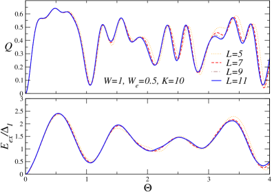
Figure 12: Plot of the ratio $E_{\rm ex}/\Delta_{\cal I}(L)$— the energy exchange is defined in Eq. (58)—and of the decoherence factor $Q$, defined in Eq. (59), versus $\Theta$. $\Delta_{\cal I}(L)\sim L^{-z}$ is the gap of the Ising chain (2) at $g=g_{\cal I}$. For each $L$, we fix $g$, $g_{e}$, and $\kappa$, so that the equilibrium scaling variables defined in Eq. (31) take the values $W=1$, $W_{e}=0.5$, and $K=10$ (therefore, as $L$ increases, $g,g_{e}\to 1$ and $\kappa\to 0$). The collapse of the results for different sizes on a single curve supports the dynamic FSS relations Eqs. (62) and (64).

VII Conclusions

We have discussed the quantum behavior of an open many-body system ${\cal S}$ interacting with a surrounding many-body environment ${\cal E}$, assuming that the global system is a pure state $|\Psi_{{\cal S}\oplus{\cal E}}(t)\rangle$ that evolves unitarily. As a paradigmatic model, we consider two coupled one-dimensional Ising chains with Hamiltonian (1), see Fig. 1, but the theoretical predictions apply to general $d$-dimensional Ising systems. One of the chains plays the role of the open system ${\cal S}$ under observation, while the other one plays the role of environment ${\cal E}$. The two chains interact by means of the Hamiltonian term $H_{\cal SE}$ defined in Eq. (4), that couples the longitudinal spin variables of both subsystems. We analyze the decoherence rate and the quantum critical behavior of the subsystem ${\cal S}$, assuming that the global system is in its ground state. We also discuss the out-of-equilibrium behavior after a sudden quench of the interaction between ${\cal S}$ and ${\cal E}$, assuming that the global system is isolated and evolves unitarily. In particular, we study how these equilibrium and out-of-equilibrium behaviors depend on the quantum phases of ${\cal E}$, when ${\cal S}$ and ${\cal E}$ are weakly coupled. A detailed RG analysis shows that three qualitatively different behaviors are observed depending on ${\cal E}$, whether it is disordered (therefore characterized by short-ranged correlations), critical (correlations are algebraically decaying) or ordered (long-range correlations). The different phases of ${\cal E}$ give rise to different FSS behaviors with respect to the coupling parameter $\kappa$ between ${\cal S}$ and ${\cal E}$

To quantify the effects of the interaction with the environment on the coherence properties of ${\cal S}$, we consider the susceptibility $\chi_{Q}$ of the decoherence factor $Q$, defined in Eq. (10). The susceptibility $\chi_{Q}$ provides a measure of the sensitivity of the coherence properties of ${\cal S}$ to the coupling with ${\cal E}$ for small value of $\kappa$. It shows a power-law divergence in the size $L$ of the system, for any state of ${\cal E}$. However, the power-law depends on the phase: $\chi_{Q}\sim L^{y_{r}}$ when ${\cal E}$ is disordered, $\chi_{Q}\sim L^{2y_{\kappa}}$ with $y_{\kappa}=y_{h}-y_{\phi}$ when ${\cal E}$ is critical, $\chi_{Q}\sim L^{2y_{h}}$ when ${\cal E}$ is ordered, where $y_{r}$ and $y_{h}$ are the RG dimensions of the leading even and odd relevant perturbations at the $(d+1)$-dimensional Ising fixed point, and $y_{\phi}$ is the RG dimension of the order-parameter field. Note that, since $y_{r}<2y_{\kappa}<2y_{h}$ in any dimension, the decoherence rate of ${\cal S}$ becomes larger and larger, moving from a disordered to an ordered environment ${\cal E}$. For example, for one-dimensional systems we have $y_{r}=1$, $2y_{\kappa}=7/2$ and $2y_{h}=15/4$. Numerical results for coupled Ising chains, obtained by means of exact-diagonalization and DMRG computations, nicely support the scaling behaviors put forward in this paper.

We have also discussed how the equilibrium scaling behaviors can be extended to out-of-equilibrium dynamic processes, for instance, to protocols entailing a sudden quench of the coupling between ${\cal S}$ and ${\cal E}$, see Sec. VI. In particular, for a soft quench we conjecture out-equilibrium FSS laws that extend those valid at equilibrium. They are obtained by simply adding an additional dependence on the time scaling variable $\Theta=t\Delta_{\cal I}(L)$ (where $\Delta_{\cal I}\sim L^{-z}$ is the gap at the critical point of a quantum Ising system) to the equilibrium FSS relations.

In our analysis we focused on the behavior of ${\cal S}$ and ${\cal E}$, always assuming that the subsystem ${\cal S}$ under observation is close to criticality. It would be interesting to investigate the same issues when the subsystem ${\cal S}$ is the first-order transition region, i.e., for $g<g_{\cal I}$. In this regime, FSS behaviors emerge as well, although they turn out to significantly depend on the nature of the boundary conditions, see, e.g., Refs. CNPV-14 ; CPV-15 ; PRV-18-fo ; PRV-18-qu ; PRV-18-def ; PRV-20 ; RV-21 .

We stress that the scenario emerging from the study of two coupled Ising chains is expected to be quite general. Therefore, it should be straightforward to extend the analysis presented in this paper to systems ${\cal S}$ and ${\cal E}$ of different nature, different dimensionality, etc… In particular, we expect the behavior of ${\cal S}$, including the coherence properties, phase diagram and critical behavior, to be strongly dependent on the quantum phase of the environment ${\cal E}$. However, we note that our general scaling framework at the multicritical point, when both ${\cal S}$ and ${\cal E}$ develop critical modes (see Sec. IV.2), was essentially assuming a competition of critical modes characterized by equal dynamic exponents $z$, in particular $z=1$ for both subsystem criticalities. We believe that the competition of critical modes associated with different dynamic exponents may lead to further interesting features, worth being investigated.

The effects of the interactions with an environment (bath) on quantum many-body systems have been addressed, exploiting different approaches, in, e.g., Refs. CL-83 ; LCD-87 ; WTS-04 ; SWT-04 ; WVTC-05 ; YMZ-14 ; ARBA-17 ; KMSFR-17 ; WSBR-18 ; NRV-19 ; RV-20 ; RV-21 . One approach is based on the so-called Lindblad master equation BP-book ; RH-book , which allows for some types of dissipative interactions without the necessity of keeping track of the full environment dynamics, within some approximations, see, e.g., Ref. RV-21 and references therein. As shown for various systems and modelizations of the dissipative interactions within the Lindblad framework, the interaction with the environment makes the quantum critical behavior of a closed system generally unstable YMZ-14 ; NRV-19 ; RV-20 ; RV-21 , similarly to a finite temperature. Indeed, in this framework the dissipative interactions are relevant perturbations, which move the open system away from the quantum critical behavior of the isolated system. An alternative mechanism leading to dissipation is provided by the coupling of a many-body system with an infinite set of harmonic oscillators, see, e.g., Refs. CL-83 ; LCD-87 ; WTS-04 ; SWT-04 ; WVTC-05 . Also this type of dissipative interactions is a relevant perturbation of the critical behavior of isolated systems, and may lead to other types of criticality driven by dissipation. We note that our modelling, in which the global system is isolated and evolves unitarily, is physically different from the one used in the Lindblad framework or when an infinite set of oscillators is coupled with the system.

The predicted FSS behaviors put forward in this paper have been clearly observed in numerical simulations of stacked Ising chains for a relatively small number of coupled spins. For example, the scaling behavior of the decoherence factor has been observed in systems with a few tens of qubits. This suggests the possibility of devising realistic experiments with quantum simulators to address the phenomena discussed here, by means of various platforms, see, e.g., Refs. Islam-etal-11 ; Debnath-etal-16 ; Simon-etal-11 ; Labuhn-etal-16 ; Salathe-etal-15 ; Cervera-18 ; Keesling-19 .

We finally remark that the results obtained in weakly coupled $d$-dimensional quantum Ising systems also apply to the corresponding classical systems, i.e., to coupled $D$-dimensional classical Ising systems with $D=d+1$. For instance, we may consider two coupled $D$-dimensional lattice Ising systems ${\cal S}$ and ${\cal E}$, defined by the partition function

$$Z=\sum_{{\bm{s}_{\bm{x}}}}\exp(-H_{cl}/T)\,,$$ (65)

$$H_{cl}=H_{\cal S}(J)+H_{\cal E}(J_{e})+H_{\cal SE}(\kappa)\,,$$

where

$$H_{\cal S}(J)=-J\sum_{\langle{\bm{x}}{\bm{y}}\rangle}s_{{\bm{x}}}\,s_{{\bm{y}}}\,,\quad H_{\cal E}(J_{e})=-J_{e}\sum_{\langle{\bm{x}}{\bm{y}}\rangle}w_{{\bm{x}}}\,w_{{\bm{y}}}\,,$$

$$H_{\cal SE}(\kappa)=-\kappa\,\sum_{\bm{x}}s_{{\bm{x}}}\,w_{{\bm{x}}}\,.$$ (66)

Here $s_{{\bm{x}}}=\pm 1$ and $w_{{\bm{x}}}=\pm 1$ are classical spin variables associated with the sites ${\bm{x}}$ of a $D$-dimensional cubic lattice, ${\langle{\bm{x}}{\bm{y}}\rangle}$ indicates nearest-neighbour sites. Using the quantum-to-classical mapping Sachdev-book ; RV-21 , the quantum critical behavior of $d$-dimensional stacked quantum systems coincides with that of $D$-dimensional stacked classical systems with $D=d+1$. Then, using RG arguments analogous to those reported for the stacked quantum Ising systems (1) in Sec. IV and VI (in the dynamic case, one should also specify a particular dynamics, for instance, the purely relaxational dynamics HH-77 ), one can straightforwardly derive similar FSS relations for the subsystem ${\cal S}$ in the background of the environment ${\cal E}$, when ${\cal S}$ is close to criticality and the coupling $\kappa$ is sufficiently small. These scaling behaviors crucially depend on the effective phase of the environment ${\cal E}$ controlled by its parameter $J_{e}$. Although the scaling behavior is expected to be analogous, classical and quantum systems are expected to show significant quantitative differences. For instance, for $\kappa\to\infty$ the classical model turns out to be equivalent to a single classical Ising model (in the limit $\kappa\to\infty$ only configurations satisfying $s_{{\bm{x}}}=w_{{\bm{x}}}$ on all sites are allowed), with an ordered and a disordered phase separated by a standard Ising transition. In the quantum case, for large $\kappa$ the system can also be modelled by a single Ising chain, see App. B. However, the width of the paramagnetic phase shrinks as $\kappa$ increases, so that the two chains are always ordered in the limit $\kappa\to\infty$.

Appendix A Landau-Ginzburg-Wilson mean-field analysis

In this Appendix we discuss the model using the standard Landau-Ginzburg-Wilson approach. We consider a classical model in $D=d+1$ dimensions with two scalar fields $\phi_{1}$ and $\phi_{2}$, with interaction potential

$$V=\int d^{D}x\,\left[V_{2}(\phi_{1},\phi_{2})+V_{4}(\phi_{1},\phi_{2})\right]\,,$$ (67)

where

$$V_{2}(\phi_{1},\phi_{2})={r_{1}\over 2}\phi_{1}^{2}+{r_{2}\over 2}\phi_{2}^{2}+\kappa\,\phi_{1}\phi_{2}\,,$$ (68)

and $V_{4}(\phi_{1},\phi_{2})$ is the quartic potential. Cubic terms do not enter because of the symmetry under simultaneous changes of the sign of the two fields, $\phi_{1,2}\to-\phi_{1,2}$. Close to the critical point, the parameters $r_{1}$ and $r_{2}$ correspond to $g_{e}-g_{\cal I}$ and $g-g_{\cal I}$, respectively.

In the mean-field approach, the kinetic term is neglected and the transition lines are determined from the analysis of the quadratic terms. To clarify the behavior, we first perform a unitary transformation of the fields that diagonalizes the quadratic part. If $\psi_{1}$ and $\psi_{2}$ are the new fields we obtain

$$V_{2} = {1\over 4}(r_{1}+r_{2}+\delta)\psi^{2}_{1}+{1\over 4}(r_{1}+r_{2}-\delta)\psi^{2}_{2}\,,$$

$$\delta = \sqrt{(r_{1}-r_{2})^{2}+4\kappa^{2}}\,.$$ (69)

Therefore phase transitions occur for

$$r_{1}+r_{2}=\pm\delta\quad\Rightarrow\quad r_{1}r_{2}=\kappa^{2}\,.$$ (70)

This relation implies that, if one of the two systems is at criticality, for instance $r_{1}=0$, in the $(r_{2},\kappa)$ plane there is a single transition point at $r_{2}=\kappa=0$. Otherwise, we observe transition lines along which $r_{1}$ and $r_{2}$ have the same sign. In our quantum model, this implies that transitions lie in the region $g>g_{\cal I}$, $g_{e}>g_{\cal I}$, for $\kappa\not=0$. The mean-field argument also allows transition with $g<g_{\cal I}$, $g_{e}<g_{\cal I}$. However, in this case, the two systems are already ordered, and thus the additions of the coupling between the two systems would simply increase the order, without giving rise to critical transitions.

To understand the nature of the transitions, we should analyze the quartic potential. We do this analysis for the simple case, in which the model is also symmetric under the exchange of the two Ising fields (in the quantum model it corresponds to $g_{e}=g$). In the presence of this additional symmetry, the quartic potential is given by

$$V_{4}=a_{1}(\phi^{4}_{1}+\phi_{2}^{4})+a_{2}(\phi^{2}_{1}+\phi_{2}^{2})\phi_{1}\phi_{2}+a_{3}\phi_{1}^{2}\phi_{2}^{2}\,.$$ (71)

In terms of the fields $\psi_{i}$ it becomes

$$V_{4} = {1\over 4}(2a_{1}+a_{3}+a_{2}s_{\kappa})\psi_{1}^{4}+{1\over 4}(2a_{1}+a_{3}-a_{2}s_{\kappa})\psi_{1}^{4}$$ (72)

$$+{1\over 2}(6a_{1}-a_{3})\psi_{1}^{2}\psi_{2}^{2}\,,$$

where $s_{\kappa}=\kappa/|\kappa|$. The two ${\mathbb{Z}}_{2}$ symmetries of the original model imply that the system is invariant under independent changes of the sign of $\psi_{1}$ and $\psi_{2}$, which explains why there are no odd powers of $\psi_{i}$ in the quartic potential. Thus, in the symmetric case, the generic model corresponds to two Ising systems with an energy-energy coupling. For systems in $D=3$ dimensions there is the possibility of a symmetry enlargement at the multicritical point—the ${\mathbb{Z}}_{2}\otimes{\mathbb{Z}}_{2}$ invariance enlarges to O(2) FN-74 ; NKF-74 ; CPV-03 ; BPV-22 . In $D=2$ dimension the energy-energy interaction is marginal at the O(2) fixed point and thus a more complex behavior can be obtained. As we have discussed in the text, the latter possibility can be realized by adding a coupling between the transverse spins, such as in Eq. (7). The model we consider has a decoupled multicritical point, i.e., it corresponds to $a_{3}=6a_{1}$. Thus, the effective model is simply the sum of two noninteracting Ising systems. Thus, at fixed $\kappa\not=0$, the transition is obtained by tuning $g=g_{e}$ at a critical point $g_{c}(\kappa)$. The quantity $g-g_{c}(\kappa)$ is a thermal Ising scaling field. Nothing would change for $g\not=g_{e}$. Odd terms $\psi_{1}\psi_{2}^{3}$ and $\psi_{3}\psi_{1}$, would now be present. However, for $\kappa\not=0$, only one field is critical. The noncritical field should be integrated out and it would give rise to even contributions in the critical field. Thus, we predict all deviations from the critical point to represent Ising thermal scaling fields.

Appendix B Large-$\kappa$ and large-$g_{e}$ transitions

In this Appendix, we discuss the behavior of the system for large values of $\kappa$ and for large values of $g_{e}$.

Let us first consider the limit $\kappa\to\infty$ at fixed $g$ and $g_{e}$. If the system is in the global ground state, the coupling term $H_{\cal SE}$ forces the ${\cal S}$ and ${\cal E}$ spins on the same site to be aligned. Therefore, we can simply consider the problem in the reduced Hilbert space obtained by only considering the states $|++\rangle_{1}$ and $|--\rangle_{1}$ on each site. Here $|++\rangle_{1}$ and $|--\rangle_{1}$ are the single-site eigenvectors of $\sigma^{(1)}$ and $\tau^{(1)}$: $\sigma^{(1)}|++\rangle_{1}=+|++\rangle_{1}$, $\tau^{(1)}|++\rangle_{1}=+|++\rangle_{1}$, and $\sigma^{(1)}|--\rangle_{1}=-|--\rangle_{1}$, $\tau^{(1)}|--\rangle_{1}=-|--\rangle_{1}$. The computation of the ground state of the total Hamiltonian in this reduced space is trivial. The ground state is independent of $g_{e}$ and $g$ and doubly degenerate: a basis is provided by the two fully ordered configurations.

In this derivation we have assumed that $g$ and $g_{e}$ are fixed as $\kappa$ increases, i.e. we are in the limit $g,g_{e}\ll\kappa$. However, it is equally possible that $\kappa$ is large, but still smaller than $g$, i.e., the couplings satisfy $g_{e}\ll\kappa\ll g$. In this case, the relevant states will be eigenstates of $\sigma^{(3)}_{x}$ on each site. The coupling Hamiltonian $\kappa$ does not play any role—the two systems decouple—and one has an effectively disordered subsystem $\cal S$. Thus, for $\kappa$ and $g$ large, depending on their relative size, $\cal S$ can be either ordered or disordered. We thus expect a transition when $\kappa$ and $g$ are both large, but of the same order.

For convenience, we will adopt below the following notation for the single-site states. We indicate with $|++\rangle$, $|+-\rangle$,$|-+\rangle$, $|--\rangle$ the single-site eigenvectors of $\sigma^{(3)}$ and $\tau^{(3)}$, respectively. For instance, $|+-\rangle$ satisfies $\sigma^{(3)}|+-\rangle=+|+-\rangle$ and $\tau^{(3)}|+-\rangle=-|+-\rangle$. If both $\kappa$ and $g$ are large, the relevant Hilbert space can be obtained by diagonalizing the single-site Hamiltonian, i.e., by considering

$$H_{ss}=-g\sigma^{(3)}-g_{e}\tau^{(3)}-\kappa\sigma^{(1)}\tau^{(1)}.$$ (73)

For $\kappa,g\gg g_{e}\sim 1$ the relevant eigenstates are

$$\psi_{0} = {A\over\sqrt{1+A^{2}}}|++\rangle+{1\over\sqrt{1+A^{2}}}|--\rangle,$$

$$\psi_{1} = {A\over\sqrt{1+A^{2}}}|+-\rangle+{1\over\sqrt{1+A^{2}}}|-+\rangle,$$ (74)

where, neglecting corrections of order $g_{e}/g$, we have

$$A={g\over\kappa}+\sqrt{1+{g^{2}\over\kappa^{2}}}.$$ (75)

The gap is

$$\Delta=E(\psi_{1})-E(\psi_{0})={2g\over\sqrt{g^{2}+\kappa^{2}}}g_{e},$$ (76)

where we have only kept the leading term in $g_{e}$. The other two states have energy differences of order $g,\kappa$, with respect to the ground state. The previous expression shows the presence of two different regimes, in agreement with the previous discussion. If $\kappa/g\to\infty$, $\Delta$ goes to zero, so that the two states become degenerate. Moreover, since $A\to 1$, the combinations $\psi_{0}\pm\psi_{1}$ correspond to the aligned states we have discussed above. If instead $g/\kappa\to\infty$, the system is gapped and the ground state corresponds to a paramagnetic $\cal S$.

To discuss the generic case, let us note that, for $g,\kappa\gg g_{e}$, on each site the relevant Hilbert space consists of the two states $\psi_{0}$ and $\psi_{1}$. If we associate the vector $(1,0)$ to $\psi_{0}$ and the vector $(0,1)$ to $\psi_{1}$, we can write the local Hamiltonian in this restricted Hilbert space as

$$H_{\rm loc}=-{\Delta\over 2}\lambda^{(3)}+E_{m}\qquad\lambda^{(3)}=\begin{pmatrix}1&0\\ 0&-1\end{pmatrix}$$ (77)

where $\lambda^{(3)}$ is a Pauli matrix and $E_{m}=[E(\psi_{0})+E(\psi_{1})]/2$. The hopping part of the full Hamiltonian can be similarly written as an effective hopping term involving $\lambda^{(1)}_{\bm{x}}\lambda^{(1)}_{\bm{y}}$ on neighbouring sites. Thus, apart from an additive constant, we end up with an effective Ising chain with Hamiltonian

$$H=-J_{\rm eff}\sum_{(\bm{x}y)}\lambda^{(1)}_{\bm{x}}\lambda^{(1)}_{\bm{y}}-{\Delta\over 2}\sum_{\bm{x}}\lambda^{(3)}_{\bm{x}},$$ (78)

where

$$J_{\rm eff}={1+6A^{2}+A^{4}\over(1+A^{2})^{2}}.$$ (79)

Therefore, we predict a transition for

$$J_{\rm eff}={\Delta\over 2}.$$ (80)

This equation depends only on the ratio $\kappa/g$ and $g_{e}$. Therefore, we predict

$$\kappa_{c}(g,g_{e})=\alpha(g_{e})g\,\quad{\rm for}\;\kappa,g\gg g_{e}\,.$$ (81)

Numerically, we find $\alpha(g_{e})=0.931,1.99,5.00$ for $g_{e}=2,4,10$. For large values of $g_{e}$, we have approximately $\alpha(g_{e})\approx g_{e}/2(1-2/g_{e}^{-4})$. For $g_{e}\to 1$ we have $\alpha(g_{e})\approx\sqrt{2\over 3}(g_{e}-1)^{1/2}$. As expected, no solution exists for $g_{e}<1$.

We have performed a numerical check of the prediction by computing $\kappa_{c}(g)$ for $g_{e}=2$ and several values of $g$. Data for $g\geq 2$ are well fitted by $\kappa_{c}(g)\approx ag+b$, with $a=0.94(1)$ and $b=-0.5(1)$. The estimate of $a$ is in agreement with the prediction 0.931, obtained above.

The behavior for large values of $g_{e}$ at fixed $\kappa$ and $g$ can be discussed analogously. For $g_{e}\to\infty$, as discussed in Sec. IV.1.2, the subsystems $\cal E$ and $\cal S$ are decoupled and $g_{c}(\kappa)=1$ for all values of $\kappa$. We wish now to compute the corrections to this result. We proceed as before, diagonalizing the local single-site Hamiltonian. For $g_{e}\to\infty$ the relevant eigenvectors are

$$\psi_{0} = {B_{1}\over\sqrt{1+B_{1}^{2}}}|++\rangle+{1\over\sqrt{1+B_{1}^{2}}}|--\rangle,$$

$$\psi_{1} = {B_{2}\over\sqrt{1+B_{2}^{2}}}|+-\rangle+{1\over\sqrt{1+B_{2}^{2}}}|-+\rangle,$$ (82)

where, to leading order in $g_{e}$, we have

$$B_{1}={2g_{e}\over\kappa},\qquad B_{2}={\kappa\over 2g_{e}}.$$ (83)

As before, the states $|++\rangle$, $\ldots$, are eigenstates of $\sigma^{(3)}$ and $\tau^{(3)}$. In the same limit the gap is

$$\Delta\approx 2g-{g\kappa^{2}\over g_{e}^{2}}.$$ (84)

To complete the calculation, we should compute the coupling $J_{\rm eff}$ that parameterizes the hopping term. We find

$$J_{\rm eff}=1+{4B_{1}B_{2}\over(B_{1}^{2}+1)(B_{2}^{2}+1)}\approx 1+{\kappa^{2}\over g_{e}^{2}}.$$ (85)

Requiring $\Delta/2=J_{\rm eff}$ we obtain

$$g_{c}(\kappa)=1+{3\over 2g_{e}^{2}}\kappa^{2}.$$ (86)

which is valid as long as $\kappa\ll g_{e}$.

References

- (1) W. H. Zurek, Decoherence, einselection, and the quantum origins of the classical, Rev. Mod. Phys. 75, 715 (2003).
- (2) M. A. Nielsen and I. L. Chuang, Quantum Computation and Quantum Information, (Cambridge University Press, Cambridge, 2010).
- (3) N. Lambert, Y.-N. Chen, Y.-C. Cheng, C.-M. Li, G.-Y.Chen, and F. Nori, Quantum biology, Nat. Phys. 9, 10 (2013).
- (4) S. Sachdev, Quantum Phase Transitions, (Cambridge University, Cambridge, England, 1999).
- (5) D. Rossini and E. Vicari, Coherent and dissipative dynamics at quantum phase transitions, Phys. Rep. 936, 1 (2021).
- (6) W. H. Zurek, Environment-induced superselection rules, Phys. Rev. D 26, 1862 (1982).
- (7) F. M. Cucchietti, J. P. Paz, and W. H. Zurek, Decoherence from spin environments, Phys. Rev. A 72, 052113 (2005).
- (8) H. T. Quan, Z. Song, X. F. Liu, P. Zanardi, and C. P. Sun, Decay of Loschmidt Echo Enhanced by Quantum Criticality, Phys. Rev. Lett. 96, 140604 (2006).
- (9) D. Rossini, T. Calarco, V. Giovannetti, S. Montangero, and R. Fazio, Decoherence induced by interacting quantum spin baths, Phys. Rev. A 75, 032333 (2007).
- (10) F. M. Cucchietti, S. Fernandez-Vidal, and J. P. Paz, Universal decoherence induced by an environmental quantum phase transition, Phys. Rev. A 75, 032333 (2007).
- (11) C. Cormick and J. P. Paz, Decoherence induced by a dynamic spin environment: The universal regime, Phys. Rev. A 77, 022317 (2008).
- (12) W. H. Zurek, Quantum Darwinism, Nat. Phys. 5, 181 (2009).
- (13) B. Damski, H. T. Quan, and W. H. Zurek, Critical dynamics of decoherence, Phys. Rev. A 83, 062104 (2011).
- (14) T. Nag, U. Divakaran, and A. Dutta, Scaling of the decoherence factor of a qubit coupled to a spin chain driven across quantum critical points, Phys. Rev. B 86, 020401(R) (2012).
- (15) S. Suzuki, T. Nag, and A. Dutta, Dynamics of decoherence: Universal scaling of the decoherence factor, Phys. Rev. A 93, 012112 (2016).
- (16) E. Vicari, Decoherence dynamics of qubits coupled to systems at quantum transitions, Phys. Rev. A 98, 052127 (2018).
- (17) E. Fiorelli, A. Cuccoli, and P. Verrucchi, Critical slowing down and entanglement protection, Phys. Rev. A 100, 032123 (2019).
- (18) D. Rossini and E. Vicari, Scaling of decoherence and energy flow in interacting quantum many-body systems, Phys. Rev. A 99, 052113 (2019).
- (19) A. Franchi, D. Rossini, and E. Vicari, Quantum many-body spin rings coupled to ancillary spins: The sunburst quantum Ising model, Phys. Rev. E 105, 054111 (2022).
- (20) A. Franchi, D. Rossini, and E. Vicari, Decoherence and energy flow in the sunburst quantum Ising model, J. Stat. Mech. (2022) 083103.
- (21) E. Fradkin, -Color Ashkin-Teller Model in Two Dimensions: Solution in the Large- Limit, Phys. Rev. Lett. 53, 1967 (1984).
- (22) R. Shankar, Ashkin-Teller and Gross-Neveu Models: New Relations and Results, Phys. Rev. Lett. 55, 453 (1985)
- (23) A. Pelissetto and E. Vicari, Critical phenomena and renormalization group theory, Phys. Rep. 368, 549 (2002).
- (24) R. Guida and J. Zinn-Justin, Critical exponents of the N-vector model, J. Phys. A 31, 8103 (1998).
- (25) M. Campostrini, A. Pelissetto, P. Rossi, and E. Vicari, 25th-order high-temperature expansion results for three-dimensional Ising-like systems on the simple-cubic lattice Phys. Rev. E 65, 066127 (2002).
- (26) M. Hasenbusch, A finite size scaling study of lattice models in the three-dimensional Ising universality class, Phys. Rev. B 82, 174433 (2010).
- (27) F. Kos, D. Poland, D. Simmons-Duffin, and A. Vichi, Precision islands in the Ising and O() models, J. High Energy Phys. 08, 036 (2016).
- (28) M. V. Kompaniets and E. Panzer, Minimally subtracted six-loop renormalization of O()-symmetric theory and critical exponents, Phys. Rev. D 96, 036016 (2017).
- (29) M. Hasenbusch, Restoring isotropy in a three-dimensional lattice model: The Ising universality class, Phys. Rev. B 104, 014426 (2021).
- (30) M. Fishman, Steven R. White, and E. Miles Stoudenmire, The ITensor Software Library for Tensor Network Calculations, arXiv 2007.14822
- (31) F. J. Wegner, The critical state, general aspects, in: C. Domb, J.L. Lebowitz (Eds.), Phase Transitions and Critical Phenomena, vol. 6, Academic Press, London, 1976, p. 7.
- (32) M. Campostrini, A. Pelissetto, and E. Vicari, Finite-size scaling at quantum transitions, Phys. Rev. B 89, 094516 (2014).
- (33) M. E. Fisher and D. R. Nelson, Spin Flop, Supersolids, and Bicritical and Tetracritical Points, Phys. Rev. Lett. 32, 1350 (1974).
- (34) D. R. Nelson, J. M. Kosterlitz, and M. E. Fisher, Renormalization-Group Analysis of Bicritical and Tetracritical Points Phys. Rev. Lett. 33, 813 (1974); J. M. Kosterlitz, D. R. Nelson, and M. E. Fisher, Bicritical and tetracritical points in anisotropic antiferromagnetic systems, Phys. Rev. B 13, 412 (1976).
- (35) P. Calabrese, A. Pelissetto, and E. Vicari, Multicritical behavior of -symmetric systems, Phys. Rev. B 67, 054505 (2003).
- (36) C. Bonati, A. Pelissetto, and E. Vicari, Multicritical behavior of the three-dimensional gauge Higgs model, Phys. Rev. B 105, 165138 (2022).
- (37) F. B. Ramos, M. Lencsès, J. C. Xavier, and R. G. Pereira, Confinement and bound states of bound states in a transverse-field two-leg Ising ladder, Phys. Rev. B 102, 014426 (2020).
- (38) A. LeClair, A. Ludwig, and G. Mussardo, Integrability of coupled conformal field theories, Nucl. Phys. B 512, 523 (1998).
- (39) M. Campostrini, J. Nespolo, A. Pelissetto, and E. Vicari, Finite-size scaling at first-order quantum transitions, Phys. Rev. Lett. 113, 070402 (2014); Finite-size scaling at first-order quantum transitions of quantum Potts chains, Phys. Rev. E 91, 052103 (2015).
- (40) M. Campostrini, A. Pelissetto, and E. Vicari, Quantum transitions driven by one-bond defects in quantum Ising rings, Phys. Rev. E 91, 042123 (2015); Quantum Ising chains with boundary terms, J. Stat. Mech. (2015) P11015.
- (41) A. Pelissetto, D. Rossini, and E. Vicari, Finite-size scaling at first-order quantum transitions when boundary conditions favor one of the two phases, Phys. Rev. E 98, 032124 (2018).
- (42) J. Dziarmaga, Dynamics of a quantum phase transition and relaxation to a steady state, Adv. Phys. 59, 1063 (2010).
- (43) A. Polkovnikov, K. Sengupta, A. Silva, and M. Vengalattore, Colloquium: Nonequilibrium dynamics of closed interacting quantum systems, Rev. Mod. Phys. 83, 863 (2011).
- (44) I. M. Georgescu, S. Ashhab, and F. Nori, Quantum Simulation, Rev. Mod. Phys. 86 154 (2014).
- (45) M. A. Nielsen and I. L. Chuang, Quantum Computation and Quantum Information (Cambridge University Press, Cambridge, 2010)
- (46) N. Lambert, Y.-N. Chen, Y.-C. Cheng, C. M. Li, G. Y. Chen, and F. Nori, Quantum biology, Nat. Phys. 9 10 (2013).
- (47) J. Goold, M. Huber, A. Riera, L. del Rio, and P. Skrzypczyk, The role of quantum information in thermodynamics, J. Phys. A: Math. Theor. 49 143001 (2016).
- (48) S. Vinjanampathy and J. Anders, Quantum Thermodynamics, Contemp. Phys. 57 545 (2016).
- (49) F. Campaioli, F. A. Pollock, and S. Vinjanampathy, in Thermodynamics in the Quantum Regime, edited by Binder F, Correa L A, Gogolin C, Anders J and Adesso G, 2018 (Springer, New York), pp. 207–225
- (50) A. Pelissetto, D. Rossini, and E. Vicari, Dynamic finite-size scaling after a quench at quantum transitions, Phys. Rev. E 97, 052148 (2018).
- (51) T. W. B. Kibble, Some implications of a cosmological phase transition, Phys. Rep. 67, 183 (1980).
- (52) W. H. Zurek, Cosmological Experiments in Superfluid Helium?, Nature 317, 505 (1985).
- (53) W. H. Zurek, Cosmological experiments in condensed matter systems, Phys. Rep. 276, 177 (1996).
- (54) A. Chandran, A. Erez, S. S. Gubser, and S. L. Sondhi, Kibble-Zurek problem: Universality and the scaling limit, Phys. Rev. B 86, 064304 (2012).
- (55) F. Tarantelli and E. Vicari, Out-of-equilibrium dynamics arising from slow round-trip variations of Hamiltonian parameters across quantum and classical critical points, Phys. Rev. B 105, 235124 (2022).
- (56) A. Pelissetto, D. Rossini, and E. Vicari, Out-of-equilibrium dynamics driven by localized time-dependent perturbations at quantum phase transitions, Phys. Rev. B 97, 094414 (2018).
- (57) A. Pelissetto, D. Rossini, and E. Vicari, Scaling properties of the dynamics at first-order quantum transitions when boundary conditions favor one of the two phases, Phys. Rev. E 102, 012143 (2020).
- (58) A. O. Caldeira and A. J. Leggett, Quantum tunnelling in a dissipative system, Ann. Physics 149, 374 (1983).
- (59) A.J. Leggett, S. Chakravarty, A.T. Dorsey, M.P.A. Fisher, A. Garg, and W. Zwerger, Dynamics of the dissipative two-state system, Rev. Mod. Phys. 59, 1 (1987); Rev. Mod. Phys. 67, 725 (Erratum).
- (60) P. Werner, M. Troyer, and S. Sachdev, Quantum spin chains with site dissipation, J. Phys. Soc. Jpn. Suppl. 74, 67 (2005).
- (61) S. Sachdev, P. Werner, and M. Troyer, Universal conductance of nanowires near the superconductor-metal quantum transition, Phys. Rev. Lett. 92, 237003 (2004).
- (62) P. Werner, K. Völker, M. Troyer, and S. Chakravarty, Phase diagram and critical exponents of a dissipative Ising spin chain in a transverse magnetic field, Phys. Rev. Lett. 94, 047201 (2005).
- (63) S. Yin, P. Mai, and F. Zhong, Nonequilibrium quantum criticality in open systems: The dissipation rate as an additional indispensable scaling variable, Phys. Rev. B 89, 094108 (2014).
- (64) O. Alberton, J. Ruhman, E. Berg, and E. Altman, Fate of the One Dimensional Ising Quantum Critical Point Coupled to a Gapless Boson, Phys. Rev. B 95, 075132 (2017).
- (65) M. Keck, S. Montangero, G. E. Santoro, R. Fazio, and D. Rossini, Dissipation in adiabatic quantum computers: lessons from an exactly solvable model, New. J. Phys. 19, 113029 (2017).
- (66) H. Weisbrich, C. Saussol, W. Belzig, and G. Rastelli, Decoherence in the quantum Ising model with transverse dissipative interaction in the strong coupling regime, Phys. Rev. A 98, 052109 (2018).
- (67) D. Nigro, D. Rossini, and E. Vicari, Competing coherent and dissipative dynamics close to quantum criticality, Phys. Rev. A 100, 052108 (2019); D. Rossini and E. Vicari, Scaling behavior of stationary states arising from dissipation at continuous quantum transitions, Phys. Rev. B 100, 174303 (2019).
- (68) D. Rossini and E. Vicari, Dynamic Kibble-Zurek scaling framework for open dissipative many-body systems crossing quantum transitions, Phys. Rev. Research 2, 023211 (2020).
- (69) H.-P. Breuer and F. Petruccione, The Theory of Open Quantum Systems (Oxford University Press, New York, 2002).
- (70) A. Rivas and S. F. Huelga, Open Quantum System: An Introduction (SpringerBriefs in Physics, Springer, 2012).
- (71) R. Islam, E. E. Edwards, K. Kim, S. Korenblit, C. Noh, H. Carmichael, G.-D. Lin, L.-M. Duan, C.-C. Joseph Wang, J. K. Freericks, and C. Monroe, Onset of a quantum phase transition with a trapped ion quantum simulator, Nat. Commun. 2, 377 (2011).
- (72) S. Debnath, N. M. Linke, C. Figgatt, K. A. Landsman, K. Wright, and C. Monroe, Demonstration of a small programmable quantum computer with atomic qubits, Nature 536, 63 (2016).
- (73) J. Simon, W. S. Bakr, R. Ma, M. E. Tai, P. M. Preiss, and M. Greiner, Quantum simulation of antiferromagnetic spin chains in an optical lattice, Nature 472, 307 (2011).
- (74) H. Labuhn, D. Barredo, S. Ravets, S. de Leseleuc, T. Macri, T. Lahaye, and A. Browaeys, Tunable two-dimensional arrays of single Rydberg atoms for realizing quantum Ising models, Nature 534, 667 (2016).
- (75) Y. Salathé, M. Mondal, M. Oppliger, J. Heinsoo, P. Kurpiers, A. Potocnik, A. Mezzacapo, U. Las Heras, L. Lamata, E. Solano, S. Filipp, and A. Wallraff, Digital quantum simulation of spin models with circuit quantum electrodynamics, Phys. Rev. X 5, 021027 (2015).
- (76) A. Cervera-Lierta, Exact Ising model simulation on a quantum computer, Quantum 2, 114 (2018).
- (77) A. Keesling, A. Omran, H. Levine, H. Bernien, H. Pichler, S. Choi, R. Samajdar, S. Schwartz, P. Silvi, S. Sachdev, P. Zoller, M. Endres, M. Greiner, V. Vuletic, and M. D. Lukin, Quantum Kibble–Zurek mechanism and critical dynamics on a programmable Rydberg simulator, Nature (London) 568, 207 (2019).
- (78) P. C. Hohenberg and B. I. Halperin, Theory of dynamic critical phenomena, Rev. Mod. Phys. 49, 435 (1977).