From the gates of the abyss: Frequency- and polarization-dependent lensing of gravitational waves in strong gravitational fields

Abstract

The propagation of gravitational waves can be described in terms of null geodesics by using the geometrical optics approximation. However, at large but finite frequencies the propagation is affected by the spin-orbit coupling corrections to geometrical optics, known as the gravitational spin Hall effect. Consequently, gravitational waves follow slightly different frequency- and polarization-dependent trajectories, leading to dispersive and birefringent phenomena. We study the potential for detecting the gravitational spin Hall effect in hierarchical triple black hole systems, consisting of an emitting binary orbiting a more massive body acting as a gravitational lens. We calculate the difference in time of arrival with respect to the geodesic propagation and find that it follows a simple power-law dependence on frequency with a fixed exponent. We calculate the gravitational spin Hall-corrected waveform and its mismatch with respect to the original waveform. The waveform carries a measurable imprint of the strong gravitational field if the source, lens, and observer are sufficiently aligned, or for generic observers if the source is close enough to the lens. We present constraints on dispersive time delays from GWTC-3, translated from limits on Lorentz invariance violation. Finally, we address the sensitivity of current and future ground detectors to dispersive lensing. Our results demonstrate that the gravitational spin Hall effect can be detected, providing a novel probe of general relativity and the environments of compact binary systems.

I Introduction

The first detection of GW – GW150914 – by the Advanced LIGO observatory marked the beginning of the new era of gravitational-wave astronomy [1, 2]. GW carry information about their source, but also imprints of the spacetime on which they travel. Observable sources of GW emit over a wide range of frequencies [3]. As an example, the aforementioned GW150914 was detected from $\sim 35$ to $250\,\mathrm{Hz}$. Its wavelength and that of any signal detectable by LVK, remains orders of magnitude larger than that of the longest EM signal capable of crossing the atmosphere ($\sim 10\,\mathrm{MHz}$). Therefore, GW have the potential to detect novel propagation effects at low frequencies, particularly when their wavelength approaches characteristic lengths of physical systems – e.g. the Schwarzschild radius of a black hole or other gravitational lens. In these cases, the propagation of GW might deviate slightly from the standard predictions of GO [4, 5, 6].

The GO approximation assumes that the wavelength is negligible compared to all other length scales of the system. Mathematically, this is the infinite frequency limit in which the evolution of either Maxwell or linearized gravity field equations is approximated by a set of ODE instead of a set of partial differential equations. In this approximation, rays propagate along null geodesics, and the evolution of the field is approximated by transport equations along rays. Effects beyond the GO approximation are well known in optics, where spin-orbit coupling leads to polarization-dependent propagation of EM wave packets [9, 10, 11, 12, 13, 14, 15, 16, 17, 18]. This is known as the spin Hall effect of light [7, 19] and has been observed in several experiments [15, 17]. A similar effect – the GSHE [20, 21, 22, 23, 24, 25, 26, 27] – was predicted for wave packets propagating in curved spacetime and has been widely studied using various theoretical methods [28, 29, 30, 31, 32, 33, 22, 34, 23, 24, 35, 36, 20, 37, 21, 38, 39, 40, 41, 42] (see Refs. [43, 44] for a review and introduction). In this paper, we consider the GSHE of GW propagating on a curved background spacetime, as presented in Refs. [24, 26].

The GSHE is described by a set of effective ray equations that represent the propagation of a gravitational wave packet energy centroid up to first order in wavelength, derived as a higher-order GO approximation using a WKB ansatz. Within this formalism, the wave packets undergo frequency- and polarization-dependent deviations from the GO trajectory, which can be viewed as a manifestation of the spin-orbit coupling via the Berry curvature. Moreover, the deviations are described by the same effective ray equations for both EM and linearized gravitational fields [22, 24].

GW offer the best chance to probe the GSHE. The GSHE emerges as a first-order perturbation in the ratio between wavelength and the background gravitational field length scale – the Schwarzschild radius $R_{\rm s}$. While the present day GW terrestrial observatories have a lower limit at $\sim 10\,\mathrm{Hz}$ [45], or equivalently wavelength of $\sim 10^{7}\,\mathrm{m}$, radio telescopes such as the Event Horizon telescopes observe at $\sim 1.3\times 10^{-3}\leavevmode\nobreak\ \mathrm{m}$ [46], i.e. at wavelengths orders of magnitude lower than the GW interferometers. Therefore, there is little hope of finding observable astrophysical systems where the EM radiation wavelength is comparable to the gravitational field length scale.

Another reason to search for GSHE using GW is that sources may inhabit high-curvature environments. In addition to isolated evolution of massive binary stars, GW emitting binaries may form by dynamical encounters in a dense environment, such as a globular cluster [47, 48, 49] or an AGN [50, 51, 52]. For a review of hierarchical BH formation channels, see Ref. [53]. In the AGN scenario, compact objects accumulate in the disk around a supermassive black hole [54]. Interactions with the disk would subsequently drive them towards migration traps, stable orbits where gas torques change direction [55]. Migration traps could be as close as $\lesssim 10$ Schwarzschild radii of the supermassive black hole [56]. Such a “last migration trap” may contribute up to $\sim 1$% of GW events detectable by LVK. This opens up the possibility of detecting strong field effects in GW propagation in hierarchical triple systems, wherein the emitting BH binary is sufficiently close to or orbiting around a massive third companion BH. The GSHE may be detectable in these systems, in addition to multiple images of the merger caused by the BH [57, 58, 59].

Interest in the AGN-GW connection boomed after LIGO-Virgo’s detection of GW190521 [60, 61], a binary whose primary component’s mass is in the pair instability gap [62]. Such a massive BH could not have formed from stellar evolution, pointing towards a likely dynamical origin for the binary. Furthermore, the Zwicky Transient Facility detected an EM flare in AGN J124942.3+344929 (redshift of $0.438$), $34$ days after GW190521 and with consistent sky localization. In this tentative interpretation, the BH binary would be in a migration trap with a semi-major axis of $\sim 350$ Schwarzschild radii of the supermassive black hole, and the delay between both events would be the time required for the EM radiation to emerge from the accretion disk of the AGN [63]. Although suggestive, evidence for an AGN origin of GW190521 is far from conclusive when considering LIGO-Virgo data [64, 65, 66, 67, 68] or the putative EM counterpart [69, 70].

The GSHE provides a novel test of the GW source environments, which may help establish their AGN formation channel. An advantage of this test is that it can be performed on individual observations. In contrast, other proposed methods require either LISA-like observatory [71, 72] to measure the orbit of the emitting binary around the background black hole [73, 58, 74, 75, 76] or population studies. The latter being based on binary properties (masses, spin, eccentricity) [77, 78, 79] or associating GW events with detected AGN flares [80, 70]. Although measuring the GSHE might be possible for only a small fraction of the GW events originating in AGN disks, its complementarity with other methods would yield valuable insights into BH and GW astrophysics.

The GSHE arises in Einstein’s GR [24], but it is also similar to effects emerging in theories beyond GR, and thus needs to be taken into account to correctly interpret tests of gravity with GW. A nonzero graviton mass leads to a distance and frequency-dependent propagation for all GW [81]. Some alternative theories predict environment- and polarization-dependent GW propagation speeds – the GW birefringence effect [82]. This leads to a frequency-independent time delay between the $+$ and $\times$ polarization states that may either interfere in the detector or appear as two copies of the same signal if the time delay is shorter/longer than the signal, respectively. A related effect stems from parity-breaking terms in the effective field theory of GW. Ref. [83] searched for frequency-dependent GW birefringence (between left and right polarized GW), finding that only the GW190521 observation is compatible with violation of parity. All these beyond-GR effects are related to the GSHE, although in principle distinguishable from it. Establishing a detection of the GSHE in the GW data would represent yet another test of gravity and additional evidence for GR in the strong-field regime.

We demonstrate that the GSHE can be detected in GW sources in a hierarchical triple system, in which a stellar-mass binary is close to a much more massive companion, such as in an AGN. The main observable signature of the GSHE is time delay between the high- and low-frequency components of the waveform, with a correction proportional to $\sim 1/f^{2}$ relative to geodesic propagation. Therefore, the GSHE may appear as an inconsistency between the higher and lower frequency parts of the waveform (e.g., in inspiral-merger-ringdown tests of GR). A subdominant GSHE signature is a frequency-dependent birefringence effect – a time delay between the left- and right-polarized components. GSHE-birefringence is further suppressed ($\sim 1/f^{3}$) and is likely too small to be detectable, except in fine-tuned configurations. A third signature of this scenario is the likely presence of multiple signals due to strong-field lensing by the massive BH. The relative magnification, time delay, and sign of the GSHE correction between these signals should allow for further means to probe the system configuration.

The paper is organized as follows. We begin by describing the GSHE and the numerical calculation of the time of arrival delay in Section II. In Section III, we describe the dependence of the time of arrival delay on frequency, polarization state, and the mutual position of the source and the observer. In Section III, we demonstrate the effect of the GSHE on a GW waveform and its distinguishability from an uncorrected waveform. Lastly, we discuss our findings in Section IV and conclude in Section V. Our results are also presented in a more compact form in the companion Letter, Ref. [84].

We note that $\log$ refers to a logarithm of base $10$, $x\cdot y=x^{\mu}y_{\mu}$ denotes the inner product of $4$-vectors and, unless explicitly discussing dimension-full quantities, we set the speed of light, the gravitational constant and the Kerr BH mass $M$ to unity, $c=G=M=1$.

II Methodology

We assume the existence of a GW emitter – a binary BH merger – in the vicinity of a Kerr BH, with GW ray trajectories passing through the strong-field regime of the background Kerr metric. We then calculate the observer time of arrival of the GSHE trajectories, which depends on frequency and polarization, and compare it to the geodesic time of arrival. In other words, the observer detects that the waveform modes have a frequency- and polarization-dependent time of arrival that deforms the resulting waveform.

We start by reviewing the Kerr metric and GSHE equations in Section II.1. We then present our geometric setup in Section II.2 and numerical integration in Section II.3. Finally, we characterize the GSHE time delay quantities in Section II.4 and discuss our waveform model in Section II.5.

II.1 Gravitational spin Hall equations

We consider the background spacetime of a Kerr black hole with mass $M=1$ and spin parameter $a$, described using Boyer-Lindquist coordinates $(t,r,\theta,\phi)$ [85, p.195]. The line element is

$$\begin{split}\differential s^{2}=&-\frac{\Delta}{\Sigma}\left(\differential t-a\sin^{2}\theta\differential\phi\right)^{2}+\frac{\Sigma}{\Delta}\differential r^{2}+\Sigma\differential\theta^{2}\\ &+\frac{\sin^{2}\theta}{\Sigma}\left[a\differential t-(r^{2}+a^{2})\differential\phi\right]^{2},\end{split}$$ (2.1)

where

$$\Delta =r^{2}-2Mr+a^{2},$$ (2.2a)

$$\Sigma =r^{2}+a^{2}\cos^{2}\theta.$$ (2.2b)

We also consider an orthonormal tetrad

$$e_{0} =\frac{1}{\sqrt{\Delta\Sigma}}\left[(r^{2}+a^{2})\partial_{t}+a\partial_{\phi}\right],$$ (2.3a)

$$e_{1} =\sqrt{\frac{\Delta}{\Sigma}}\partial_{r},$$ (2.3b)

$$e_{2} =\frac{1}{\sqrt{\Sigma}}\partial_{\theta},$$ (2.3c)

$$e_{3} =\frac{1}{\sin\theta\sqrt{\Sigma}}\left(a\sin^{2}\theta\partial_{t}+\partial_{\phi}\right),$$ (2.3d)

that satisfies $(e_{a})^{\mu}(e_{b})_{\mu}=\tensor{\eta}{{}_{a}{}_{b}}$, where $\tensor{\eta}{{}_{a}{}_{b}}$ is the Minkowski metric. The vectors $e_{a}$ will be used in the definition of the GSHE and for the prescription of initial conditions.

On the Kerr background spacetime, we consider GW represented by small metric perturbations and described by the linearized Einstein field equations. High-frequency GW can be described using the GO approximation [86, Sec. 35.13], in which case their propagation is determined by the null geodesics of the background spacetime. However, at high but finite frequencies, higher-order corrections to the GO approximation become important.

In this paper, we consider first order in wavelength corrections to the GO approximation, wherein the propagation of GW is frequency- and polarization-dependent. This is known as the GSHE [24], and the propagation of circularly polarized gravitational wave packets is described by the GSHE equations [24, 26]

$$\dot{x}^{\mu} =p^{\mu}+\frac{1}{p\cdot t}S^{\mu\beta}p^{\nu}\nabla_{\nu}t_{\beta},$$ (2.4a)

$$\dot{x}^{\nu}\nabla_{\nu}p_{\mu} =-\frac{1}{2}R_{\mu\nu\alpha\beta}p^{\nu}S^{\alpha\beta},$$ (2.4b)

where $x^{\mu}(\tau)$ is the worldline of the energy centroid of the wave packet, $p_{\mu}(\tau)$ is the average momentum of the wave packet, the spin tensor $S^{\alpha\beta}$ describes the angular momentum carried by the wave packet and $t^{\alpha}$ is a timelike vector field representing the $4$-velocity of the observer describing the dynamics of the wave packet. We eliminate the ODE for $p_{0}$ by enforcing the null momentum condition $p\cdot p=0$ along the worldline. For the circularly polarized wave packets that we consider here, the spin tensor is uniquely fixed as

$$S^{\alpha\beta}=\frac{\epsilon s}{p\cdot t}\varepsilon^{\alpha\beta\gamma\lambda}p_{\gamma}t_{\lambda},$$ (2.5)

where $s=\pm 2$, depending on the state of circular polarization. We note that only the product $\epsilon s$ enters the GSHE equations. Therefore, if we fix the spatial boundaries $\epsilon s$ describes a $1$-parameter bundle of trajectories whose $\epsilon s=0$ trajectory is the geodesic.

Following Ref. [24], we define the dimensionless WKB perturbation parameter $\epsilon$ as the wavelength in units of the background BH mass

$$\epsilon=\frac{\lambda}{M}=2\frac{\lambda}{R_{\rm s}},$$ (2.6)

where $\lambda$ is the wavelength of the wave packet. This can be expressed in dimension-full quantities as

$$\epsilon=\frac{c^{3}}{G}\frac{1}{fM}\approx 0.1\left(\frac{40\leavevmode\nobreak\ \mathrm{Hz}}{f}\right)\left(\frac{5\times 10^{4}M_{\odot}}{M}\right),$$ (2.7)

where $f$ is the wave packet frequency.

The GSHE equations in Eq. 2.4 depend on the choice of a timelike vector field $t^{\alpha}$. The role of this vector field has been discussed in detail in Ref. [26], where it has been shown that $t^{\alpha}$ has physical meaning only at the point of emission and the point of observation of a polarized ray. At these points, $t^{\alpha}$ can be identified with the $4$-velocity of the source and observer, respectively, and is responsible for the relativistic Hall effect [87, 88]. Nevertheless, one has to pick a smooth vector field $t^{\alpha}$ defined everywhere in the region where the GSHE equations are to be integrated. We discuss our choice of $t^{\alpha}$ in the following subsection.

II.2 Spatial configuration

We consider a static source of GW close to the BH at $\bm{x}_{\rm src}=(r_{\rm src},\theta_{\rm src},\phi_{\rm src})$ with a $4$-velocity $t^{\alpha}_{\rm src}$ and a static observer far from the BH at $\bm{x}_{\rm obs}=(r_{\rm obs},\theta_{\rm obs},\phi_{\rm obs})$ with a $4$-velocity $t^{\alpha}_{\rm obs}$. The timelike vector field $t^{\alpha}$ appearing in the GSHE equations (2.4) is chosen such that

$$\left.t^{\alpha}\right|_{\bm{x}_{\rm src}}=t^{\alpha}_{\rm src}\quad\mathrm{and}\quad\left.t^{\alpha}\right|_{\bm{x}_{\rm obs}}=t^{\alpha}_{\rm obs}.$$ (2.8)

We start with the orthonormal tetrad $e_{a}$ from Eq. 2.3 and perform a spacetime-dependent local Lorentz boost of the orthonormal tetrad such that $(e_{0})^{\alpha}$ maps to $t^{\alpha}_{\rm src}$ and $t^{\alpha}_{\rm obs}$ at $\bm{x}_{\rm src}$ and $\bm{x}_{\rm obs}$, respectively. We can express the boosted orthonormal tetrad $\tilde{e}_{a}$ as

$$\tilde{e}_{0} =\frac{e_{0}+ve_{3}}{\sqrt{1-v^{2}}},$$ (2.9a)

$$\tilde{e}_{1} =e_{1},$$ (2.9b)

$$\tilde{e}_{2} =e_{2},$$ (2.9c)

$$\tilde{e}_{3} =\frac{e_{3}+ve_{0}}{\sqrt{1-v^{2}}},$$ (2.9d)

where

$$v(r)=-\frac{a\sin{\theta_{\rm obs}}}{\sqrt{\Delta(r_{\rm obs})}}e^{-(r-r_{\rm obs})^{2}}-\frac{a\sin{\theta_{\rm src}}}{\sqrt{\Delta(r_{\rm src})}}e^{-(r-r_{\rm src})^{2}}.$$ (2.10)

The exponential factor ensures a smooth transition between $t^{\alpha}_{\rm src}$, $\tensor{e}{{}_{0}^{\alpha}}$ and $t^{\alpha}_{\rm obs}$. We identify the timelike observer vector field in the GSHE equations (2.4) as $t^{\alpha}=(\tilde{e}_{0})^{\alpha}$ and further justify the Lorentz boost in Section A.2.

For simplicity, we consider a static isotropic emitter of GW in the vicinity of a massive “lensing” BH that sources the background Kerr metric and a far static observer measuring the waveform (wave packet). The caveat of isotropic emission is relevant as the emission direction of the $\epsilon s$-parameterized bundle trajectories must be rotated with respect to the geodesic, $\epsilon=0$, emission direction by an angle $\sim\epsilon s$. In this work, we do not account for the directional dependence as it is a subdominant effect. Including it would necessitate accounting for it while generating the waveform frequency modes. The Boyer-Lindquist coordinate time $t$ can be related to the static observer’s proper time $\tau$ as

$$\tau=t\sqrt{-\left.\tensor{g}{{}_{0}{}_{0}}\right|_{\bm{x}_{\rm obs}}},$$ (2.11)

which we derive in Section A.1, with $\tensor{g}{{}_{\mu}{}_{\nu}}$ being the Kerr metric tensor. Throughout the rest of the paper, we denote the coordinate time as $t$ and the static observer proper time as $\tau$.

A signal with initial momentum $p_{\rm init}$ emitted by the static source with $4$-velocity $t_{\rm src}$ has a frequency $f_{\rm src}$ in the source frame. On the other hand, the static observer with $4$-velocity $t_{\rm obs}$ will measure the signal frequency as $f_{\rm obs}$. The observer, therefore, measures the signal redshifted by

$$\frac{\lambda_{\rm obs}}{\lambda_{\rm src}}=\frac{f_{\rm src}}{f_{\rm obs}}=\frac{t_{\rm src}\cdot p_{\rm init}}{t_{\rm obs}\cdot p_{\rm f}},$$ (2.12)

where $p_{\rm f}$ is the wave packet’s momentum when it reaches the observer. This is the common expression for gravitational redshift, which is satisfied up to first order in $\epsilon$. The $\epsilon$ dependence of the gravitational redshift originates from $p_{\rm f}$ and $p_{\rm init}$, as the initial conditions of a trajectory between two fixed spatial locations depend on $\epsilon$. We will find the $\epsilon$ dependence of the gravitational redshift to be negligible. Therefore, since this produces a uniform frequency offset and no new effect, we do not consider this further. Moreover, upon emission, the following relation is enforced,

$$t_{\rm src}\cdot p_{\rm init}=-f_{\rm src}\epsilon=-1,$$ (2.13)

where the last equality follows from Eq. 2.6. An analogue of this condition is then satisfied along the trajectory, as discussed in Ref. [26].

We parameterize $p_{\rm init}$ by a unit three-dimensional Cartesian vector $\bm{k}$ expressed in spherical coordinates where $0\leq\psi\leq\pi$ and $0\leq\rho<2\pi$ are the polar and azimuthal angle, respectively. The angles $\psi$ and $\rho$ represent the emission direction on the source celestial sphere, and we have that

$$p_{\rm init}=\tilde{e}_{0}+\sin\psi\cos\rho\tilde{e}_{1}+\sin\psi\sin\rho\tilde{e}_{2}+\cos\psi\tilde{e}_{3},$$ (2.14)

which satisfies both Eq. 2.13 and the null momentum condition $p\cdot p=0$. The initial momentum pointing towards the BH, i.e. with an initial negative radial component, may equally be parameterized with $k_{2}$ and $k_{3}$,

$$p_{\rm init}=\tilde{e}_{0}-\sqrt{1-k_{2}^{2}-k_{3}^{2}}\leavevmode\nobreak\ \tilde{e}_{1}+k_{2}\tilde{e}_{2}+k_{3}\tilde{e}_{3},$$ (2.15)

which can be related to $\psi$ and $\rho$ as

$$k_{2} =\sin\psi\sin\rho,$$ (2.16a)

$$k_{3} =\cos\psi.$$ (2.16b)

We calculate the magnification factor $\mu$ defined as the ratio of the source area to the image area [89, 90, 91]. In our case, a trajectory defines a mapping from the celestial sphere of source to the far sphere of radius $r=r_{\rm obs}$ centered at the origin, which we can write as $(\psi,\rho)\mapsto(\theta,\phi)$. The magnification $\mu$ is

$$\mu=\frac{\sin\psi\differential\psi\differential\rho}{\sin\theta\differential\theta\differential\phi}=\frac{\sin\psi}{\sin\theta}\frac{1}{\det\mathbf{J}},$$ (2.17)

where the Jacobian $\mathbf{J}$ is defined as

$$\mathbf{J}=\partialderivative{(\theta,\phi)}{(\psi,\rho)}.$$ (2.18)

The magnification scales a signal propagated along a trajectory by a factor of $\sqrt{|\mu|}$ and the signal parity is given as the sign of $\mu$, or equivalently the sign of $\det\mathbf{J}$. Therefore, as a consequence of the GSHE the magnification is dependent on frequency and polarization. We will explicitly denote this dependence as $\mu(f,s)$ and the GO magnification as $\mu_{\rm GO}$.

II.3 Numerical integration

Given a fixed source and observer, our objective is to find the connecting GSHE trajectories of the $\epsilon s$ bundle. We numerically integrate the GSHE ODE of Eq. 2.4, or the null geodesic ODE recovered by substituting $\epsilon\rightarrow 0$, starting at coordinate time $t=0$, source position $\bm{x}_{\rm src}$ and initial wave packet momentum $p_{\rm init}(\bm{k})$ as discussed in Section II.2.

The Boyer-Lindquist coordinates contain coordinate singularities at the BH horizon and the coordinate north and south poles. Therefore, we include the following premature integration termination conditions. First, the integration is terminated if a trajectory penetrates or passes sufficiently close by the BH horizon, so that its radial component satisfies

$$r\leq\Delta\mathcal{H}\left(1+\sqrt{1-a^{2}}\right),$$ (2.19)

where we set $\Delta\mathcal{H}=1+10^{-4}$. Second, we terminate trajectories whose polar angle does not satisfy $\theta_{\rm tol}\leq\theta\leq\pi-\theta_{\rm tol}$, where $\theta_{\rm tol}=10^{-5}$. Lastly, we optionally support early termination if the absolute value of the difference between the current and initial azimuthal angle $\Delta\phi=|\phi-\phi_{\rm src}|$ satisfies $\Delta\phi>\max\left(2\pi-\Delta\phi,\Delta\phi\right)$ as such solutions correspond to ones that complete more than one complete azimuthal loop around the BH. We refer to trajectories that do not completely loop around the BH as “direct”.

If no early termination condition is met, we terminate the integration when the trajectory reaches the observer’s radius $r_{\rm obs}$. The integrator then outputs $x_{\rm f}$ and $p_{\rm f}$, the location and momentum vectors of the trajectory at that instant. Typically, for each source-observer configuration, there exist at least two bundles that directly connect the source and observer, with additional bundles completely looping around the BH.

We quantify whether a choice of initial direction $\bm{k}$ (and thus initial momenta) leads to a trajectory intersecting with the observer by calculating the angular distance $\Delta\sigma$ between the observer and the integrated trajectory

$$\cos\Delta\sigma=\cos\theta_{\rm f}\cos\theta_{\rm obs}+\sin\theta_{\rm f}\sin\theta_{\rm obs}\cos\Delta\phi_{\rm f},$$ (2.20)

where $\theta_{\rm f}$ and $\phi_{\rm f}$ are the polar and azimuthal angles of the trajectory at $r_{\rm obs}$, and $\Delta\phi_{\rm f}=\phi_{\rm f}-\phi_{\rm obs}$. However, we note that in the numerical implementation we use the more accurate haversine formula for small $\Delta\sigma$ [92]. A trajectory is considered to intersect with the observer if $\Delta\sigma\rightarrow 0$ and concretely we enforce that $\Delta\sigma\leq 10^{-12}$. Given the nature of the GSHE, the initial directions of the GSHE trajectories at neighboring $\epsilon$ should lie sufficiently close to each other (or to the initial geodesic direction). Therefore, we typically begin by solving for the initial direction at the highest value of $\epsilon$ that connects the source and observer, then we solve for the $2$^nd highest value of $\epsilon$ in a restricted region of the former initial direction and repeat this process down to the smallest $\epsilon$ and the geodesic initial direction.

We first evaluate the ODE symbolically in Mathematica [93], expressing them explicitly in the Boyer-Lindquist coordinates. We then export the symbolic expressions to Julia [94] and use the DifferentialEquations.jl [95] along with Optim.jl package [96] to integrate the ODEs and optimize the initial conditions, respectively. The Jacobian in Eq. 2.18 is calculated using automatic differentiation implemented in ForwardDiff.jl [97].

II.4 Quantifying the time delay

We write the observer proper time of arrival of a GSHE trajectory emitted at coordinate time $t=0$ belonging to the n^th bundle as $\tau^{\left(n\right)}_{\rm GSHE}(\epsilon,s)$. We specifically denote the proper time of arrival of the geodesic belonging to the n^th bundle as $\tau_{\rm GO}^{\left(n\right)}$, as it corresponds to the GO limit of infinite frequency. We note that

$$\lim_{\epsilon\rightarrow 0}\tau^{\left(n\right)}_{\rm GSHE}(\epsilon,s)=\tau_{\rm GO}^{\left(n\right)}.$$ (2.21)

We will calculate the dispersive GSHE-to-geodesic time delay as

$$\Delta\tau^{\left(n\right)}(\epsilon,s)=\tau^{\left(n\right)}_{\rm GSHE}(\epsilon,s)-\tau^{\left(n\right)}_{\rm GO}.$$ (2.22)

Additionally, we will also explicitly investigate the birefringent delay between the right and left polarization states

$$\Delta\tau^{\left(n\right)}_{\rm R-L}(\epsilon)=\tau^{\left(n\right)}_{\rm GSHE}(\epsilon,s=+2)-\tau^{\left(n\right)}_{\rm GSHE}(\epsilon,s=-2).$$ (2.23)

Having fixed the background Kerr metric mass $M$, or equivalently its Schwarzschild radius $R_{\rm s}$, $\epsilon$ is inversely proportional to the wave packet’s frequency $f$. Therefore, the aforementioned time delays can be expressed directly as a function of $f$. Dimension-full units of time can be restored by multiplying the resulting expression by $R_{\rm s}/2c$.

II.5 Waveform modelling

Due to the frequency- and polarization-dependent observer proper time of arrival delay with respect to the GO propagation, $\Delta\tau$, the GSHE “delays” the circular basis frequency components of the original waveform. We write the circular basis frequency-domain unlensed waveform as $\tilde{h}_{0}(f,s)$. With the notation of Eq. 2.22, the GSHE produces a frequency-domain waveform

$$\begin{split}\tilde{h}_{\rm GSHE}(f,s)=\sum_{n}e^{-2\pi if\Delta\tau^{(n)}(f,s)}\sqrt{\left|\mu^{(n)}(f,s)\right|}\tilde{h}_{0}(f,s).\end{split}$$ (2.24)

The sum runs over the different images, i.e. bundles connecting the source and observer. $\Delta\tau^{(n)}$ is defined in Eq. 2.22, up to a constant additive factor of the earliest bundle GO time of arrival considered in the sum. The exponential encodes the frequency-dependent time delay, and the square root encodes the magnification-induced amplitude scaling.

We generate the unlensed linear basis waveform in PyCBC [98], which can equivalently be described in the circular basis. The right and left circularly polarized basis vectors, $e_{\rm R}$ and $e_{\rm L}$, can be related to the plus and cross linearly polarized basis vectors, $e_{\rm+}$ and $e_{\rm x}$, as

$$e_{\rm R} =\frac{1}{\sqrt{2}}\left(e_{\rm+}+ie_{\rm x}\right),$$ (2.25a)

$$e_{\rm L} =\frac{1}{\sqrt{2}}\left(e_{\rm+}-ie_{\rm x}\right),$$ (2.25b)

discussed, e.g. in Ref. [86].

As usual, a waveform can be inverse Fourier transformed into the time domain,

$$h(\tau)=\int\differential f\leavevmode\nobreak\ \tilde{h}(f)e^{-2\pi if\tau},$$ (2.26)

where we use $\tau$ to denote the observer proper time. The waveform and detector sensitivity are typically described in the linearly polarized basis. In it, the detector strain is described as

$$h(\tau)=F_{\rm+}h_{\rm+}(\tau)+F_{\rm x}h_{\rm x}(\tau),$$ (2.27)

where $F_{\rm+}$ and $F_{\rm x}$ is the antenna response function to the plus and cross polarization [99]. Equivalently, the detector strain can be expressed as a function of the circularly polarized waveforms upon a suitable redefinition of the antenna response function.

Beyond visually comparing the GSHE-corrected waveforms to their geodesic counterparts, we also quantify their mismatch. The mismatch between two waveforms is typically maximized over the merger time and phase. However, the GSHE leaves the high-frequency part of the waveform – the merger – unchanged. Therefore, for our purposes, we define the mismatch between $h_{\rm GO}$, the GO waveform related to the unlensed waveform by including the GO magnification $\mu_{\rm GO}$, and $h_{\rm GSHE}$ simply as

$$\mathcal{M}(h_{\rm GO},h_{\rm GSHE})=1-\frac{\langle h_{\rm GO},h_{\rm GSHE}\rangle}{\sqrt{\langle h_{\rm GO},h_{\rm GO}\rangle\langle h_{\rm GSHE},h_{\rm GSHE}\rangle}},$$ (2.28)

ignoring the merger time and phase maximization. The mismatch depends on the noise-weighted inner product between two waveforms

$$\langle a,b\rangle=\mathrm{Re}\int\frac{\tilde{a}^{*}(f)\tilde{b}(f)}{S(f)}\differential f,$$ (2.29)

where $S$ is the noise spectral density amplitude that is set by choosing a GW detector. We assume the noise to be flat across all frequencies, $S(f)=1$, as was done, e.g., in Ref. [100].

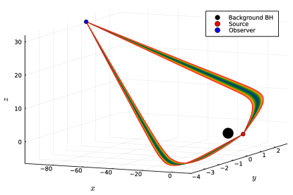
Figure 1: Two bundles of direct trajectories connecting a source at $(5\,R_{\rm s},\pi/2,0)$ and an observer at $(50\,R_{\rm s},0.4\pi,\pi)$, on the Kerr background metric with $a=0.99$. The GSHE trajectories appear as perturbations along their respective geodesic solutions. We plot trajectories with $s=\pm 2$ and $10^{-3}\leq\epsilon\leq 10^{-0.3}$, and the units along the space axes are chosen such that $R_{\rm s}=2$.

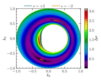
Figure 2: Dependence of the far-sphere angular distance $\Delta\sigma$ on the geodesic initial momentum ($\epsilon=0$) for a source at $(5\,R_{\rm s},\pi/2,0)$, observer at $(50\,R_{\rm s},0.4\pi,\pi)$ and $a=0.99$. We minimize $\Delta\sigma$ to find initial momenta that result in connecting trajectories. The highlighted points are the connecting initial geodesic directions, with the neighboring lines showing the $s=\pm 2$ GSHE initial directions over $10^{-3}\leq\epsilon\leq 10^{-0.3}$.

For illustration, we now express the mismatch of a single circular polarization component of a waveform. Furthermore, we assume that $\mu(f,s)=\mu_{\rm GO}$, i.e., that the magnification of the GSHE trajectories is equal to the GO magnification, which will prove to be a sufficiently good assumption. Because the GSHE correction is a phase shift in the frequency domain, we have $\langle h_{\rm GSHE},h_{\rm GSHE}\rangle=\langle h_{\rm GO},h_{\rm GO}\rangle$ and

$$\mathcal{M}(h_{\rm GO},h_{\rm GSHE},s)=1-\frac{\int\differential f|\tilde{h}_{0}(f,s)|^{2}\cos\gamma}{\int\differential f|\tilde{h}_{0}(f,s)|^{2}},$$ (2.30)

where we explicitly wrote the dependence on the circular polarization state, and we define the “mixing” angle

$$\gamma(f,s)=2\pi f\Delta\tau(f,s).$$ (2.31)

Therefore, we have that

$$\mathcal{M}(h_{\rm GO},h_{\rm GSHE},s)=\frac{1}{2}\frac{\int\differential f\leavevmode\nobreak\ \gamma^{2}|\tilde{h}_{0}(f,s)|^{2}}{\int\differential f|\tilde{h}_{0}(f,s)|^{2}}+\mathcal{O}(\gamma^{4}).$$ (2.32)

We will demonstrate in Section III.1 that the frequency dependence of $\gamma$ can be isolated from the relevant scaling set by the mutual position of the source and observer, thus further simplifying this expression.

III Results

Following the prescription of Section II, we search for bundles of connecting GSHE trajectories between a fixed source and an observer on the Kerr background metric. We investigate how the GSHE-induced time delay depends on the mutual position of the source and observer. We discover that in all cases the time delay can be well approximated as a frequency-dependent power law and that the signature of the GSHE is a frequency-dependent phase shift in the inspiral part of the observed waveform.

For each configuration, we find the initial directions of a bundle of trajectories by minimizing the angular distance $\Delta\sigma$ of Eq. 2.20. Typically, we search the range $10^{-3}\leq\epsilon\leq 10^{-1}$, with $30$ logarithmically spaced $\epsilon$ values. Everywhere but in Section III.1.3 we resort to studying only the directly connecting bundles of trajectories to simplify the interpretation. As an example, in Fig. 2 we show two directly connecting bundles. The GSHE trajectories appear as small deviations from the geodesic trajectories with fixed boundary conditions.

In Fig. 2, we plot an example dependence of $\Delta\sigma$ on the initial ingoing geodesic direction. We minimize $\Delta\sigma$ to find the initial directions that result in a connecting trajectory between a source and an observer. The empty central region indicates the initial directions that penetrate the BH horizon, delineating the BH shadow. We also overplot in Fig. 2 the GSHE initial directions upon increasing $\epsilon$ for $s=\pm 2$. If $\epsilon\rightarrow 0$ the GSHE initial direction coincides with the initial geodesic direction, otherwise it is twisted by an angle proportional to $\epsilon$.

Now we first characterize the frequency and polarization dependence of the time delay on the system configuration in Section III.1 and then address its impact on the observed waveform in Section III.2.

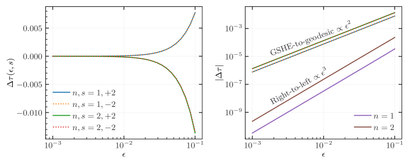
Figure 3: The dispersive GSHE-to-geodesic delay with trajectory bundles indexed by $n$ (left panel) and the logarithm of the absolute value of the GSHE-to-geodesic delay along with the right-to-left delay for each bundle (right panel) displaying the power law dependence of the delay. The source is at $(2\,R_{\rm s},\pi/2,0)$, observer at $(50\,R_{\rm s},0.4\pi,\pi)$ and $a=0.99$.

III.1 Time delay

In Fig. 3 we plot the GSHE-to-geodesic, $\Delta\tau(\epsilon,s)$, and the right-to-left, $\Delta\tau_{\rm R-L}(\epsilon)$, time of arrival delays for a particular source-observer configuration. We find that, independent of the mutual positions of the source and observer, both $\Delta\tau(\epsilon,s)$ and $\Delta\tau_{\rm R-L}(\epsilon)$ are well described by a power law. Therefore, we introduce

$$\Delta\tau(\epsilon,s) \approx\beta\epsilon^{\alpha},$$ (3.1a)

$$\Delta\tau_{\rm R-L}(\epsilon) \approx\beta_{\rm R-L}\epsilon^{\alpha_{\rm R-L}},$$ (3.1b)

for the dispersive GSHE-to-geodesic and birefringent right-to-left delay, respectively. In all cases, we find $\alpha\approx 2$ and $\alpha_{\rm R-L}\approx 3$. We note that in the former case both $\alpha$ and $\beta$ have what will turn out to be only a weak dependence on the circular polarization state. The difference between the right and left polarization results in the subdominant, but nonzero, $\Delta\tau_{\rm R-L}(\epsilon)$ delay.

The $\epsilon^{2}$ dependence of the GSHE-to-geodesic delay can be understood as follows. First, the GSHE correction to the equations of motion is proportional to $\epsilon$ and, second, to reach the same observer, the GSHE initial direction must be rotated with respect to the geodesic initial direction (see the small lines in Fig. 2). The magnitude of this rotation is proportional to $\epsilon$, therefore, altogether these two effects yield an approximate $\epsilon^{2}$ dependence. The right-to-left delay is a comparison of two perturbed solutions, which produces an $\epsilon^{3}$ dependence.

On the other hand, the proportionality factors, $\beta$ or $\beta_{\rm R-L}$, are set by the relative position of the source and observer and the BH spin. $\beta$ also contains information on the polarization state of the GW. As shown in the left panel of Fig. 3, in the case of two directly connecting bundles, one of the bundles’ GSHE trajectories (regardless of the polarization state) arrive with a positive time delay with respect to its geodesic time of arrival, while the other bundles’ GSHE trajectories arrive with a negative time delay. We verify that this holds in all configurations that we tested.

We may express $\Delta\tau$ explicitly as a function of frequency in dimension-full units of as

$$\Delta\tau\approx\beta\left(\frac{2c}{R_{\rm s}}\frac{1}{f}\right)^{\alpha-1}\frac{1}{f},$$ (3.2)

with a similar expression for the right-to-left delay $\Delta\tau_{\rm R-L}$. Thus, the right-to-left delay is suppressed relative to the GSHE-to-geodesic delay by an additional power of $2c/(R_{\rm s}f)$ and generally we have $|\beta|\gg|\beta_{\rm R-L}|$ (exemplified in Fig. 3).

Numerically, we find that the GSHE trajectories have a “blind spot” approximately on the opposite side of the BH that cannot be reached, regardless of the initial emission direction. In other words, given a source close to the BH, there are spacetime points on a sphere of large $r$ that cannot be reached by GSHE trajectories, while these points can be reached by geodesics. The location and size of the blind spot depend on the position of the source, $\epsilon$ (wavelength), polarization, and the BH spin. In the Schwarzschild metric, the blind spot is a cone whose size is $\sim 0.5\leavevmode\nobreak\ \mathrm{degrees}$ for $r_{\rm src}=5\,R_{\rm s}$ and $\epsilon=0.1$ (upper limit considered in this work). The size decreases with higher $r_{\rm src}$ and lower $\epsilon$, approaching zero when $\epsilon\rightarrow 0$ as there is no blind spot in the geodesic case. The blind spot is exactly centered on the opposite side of the BH in the Schwarzschild metric. For a source in the equatorial plane, increasing the BH spin slightly tilts the blind spot away from the equatorial plane, and its size remains approximately unchanged. We note that the presence of the blind spot is not a numerical defect and is instead a consequence of the GSHE equations. We verify this by inspecting where the GSHE trajectories intersect the far-observer sphere upon emission in all possible directions from the source and increasing the numerical accuracy. We leave a further investigation and discussion of the blind spot for future work.

We note that each of the main GSHE trajectory bundles has opposite signs of the time delay, cf. Fig. 3. The first image to be received has $\beta>0$ (i.e. low frequencies delayed w.r.t. geodesic), while the second image has $\beta<0$ (low frequencies advanced w.r.t. geodesic). As geodesics correspond to extrema of the time delay, we interpret this property as the first bundle being deformed by the GSHE into longer time delays, while the second bundle gets distorted in a way that decreases the travel time. This is analogous to standard lensing theory, where images form at extrema of the time-delay function. For a point lens, the first image corresponds to the absolute minimum and the second to a saddle point of the time delay. Angular deformations around the saddle point (as found in Fig. 2) drive the time delay closer to the global minimum, explaining the lower time delay associated with $\beta<0$. The second GSHE bundle has negative parity ($\mu<0$), which is consistent with a saddle-point image in the point-lens analogy.

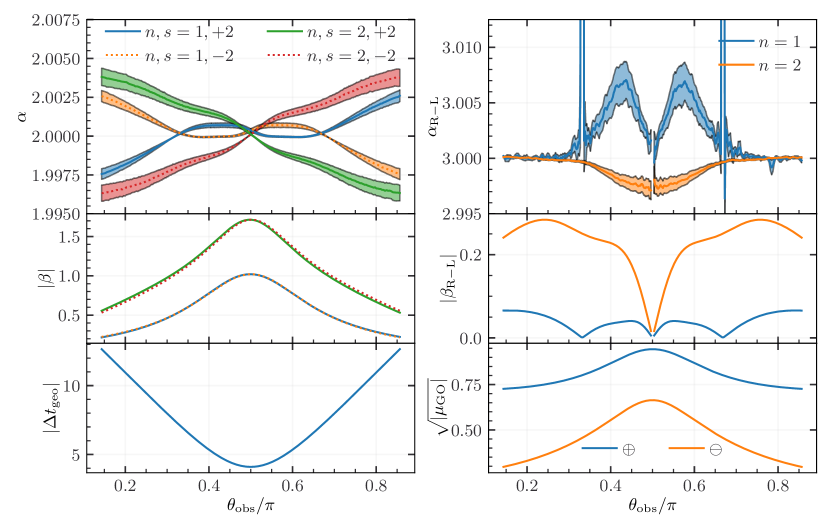
Figure 4: Time delay parametrization upon varying the polar angle of the observer $\theta_{\rm obs}$. The top row shows the power law exponent of the dispersive GSHE-to-geodesic delay $\alpha$ and of the birefringent right-to-left delay $\alpha_{\rm R-L}$. The middle row shows the corresponding power law proportionality factors $\beta$ and $\beta_{\rm R-L}$. The bottom row shows the temporal spacing of the two bundles’ geodesics $\Delta\tau_{\rm geo}$ and the geodesic magnification $\mu_{\rm GO}$ ($\oplus$ and $\ominus$ indicate positive and negative parity, respectively). The source is otherwise at $(2\,R_{\rm s},\pi/2,0)$, observer at $(50\,R_{\rm s},\theta_{\rm obs},\pi)$ and $a=0.99$. When both the source and observer are in the equatorial plane the right-to-left delay vanishes due to reflection symmetry. $\Delta\tau_{\rm geo}$ is nonzero and $\mu_{\rm GO}$ remains finite when $\theta_{\rm obs}=\pi/2$ because of the BH spin.

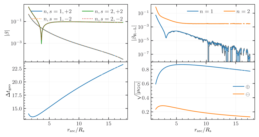
Figure 5: Time delay parametrization upon varying the source radial distance $r_{\rm src}$. Similarly to Fig. 4, the top row shows $\beta$ and $\beta_{\rm R-L}$. The bottom row shows $\Delta\tau_{\rm geo}$ and $\mu_{\rm GO}$. The source is otherwise at $(r_{\rm src},\pi/2,0)$, observer at $(50\,R_{\rm s},0.4\pi,0.75\pi)$ and $a=0.99$. We have that $\alpha\approx 2$ and $\alpha_{\rm R-L}\approx 3$. The $n=1$ bundle completes an azimuthal angle of $5\pi/4$ and is deflected in the strong-field regime of the BH. Consequently, $\beta$ approaches a constant value, however this bundle is exponentially demagnified.

We now describe the dependence of the time delay on the mutual position of the source and observer and on the spin of the BH. The BH mass enters only when we relate $\epsilon$ to frequency and restore dimension-full units of time. To demonstrate the dependence, we vary the observer’s polar angle $\theta_{\rm obs}$ and the radial distance $r_{\rm src}$ of the source from the BH. We also study the directional dependence of the GSHE, wherein we keep the source fixed but calculate the delay as a function of the emission direction. Additionally, the variation of the BH spin and observer polar angle is discussed in Appendix B. In all cases, we place the observer at $r_{\rm obs}=50\,R_{\rm s}$ after verifying that the time delay becomes approximately independent of $r_{\rm obs}$ once the observer is sufficiently far away. When we plot the power law parameters describing the time delay, we include the $1\sigma$ error bars estimated by bootstrapping. Upon varying the location of the source or observer, we associate bundles by similarity in time of arrival and initial direction.

III.1.1 Dependence on the observer polar angle

We begin by showing the dependence of the power law parameters, describing the time delay, on $\theta_{\rm obs}$ in Fig. 4. We only consider direct bundles (i.e., no complete loops around the BH) indexed by $n$. The source is kept at $(2\,R_{\rm s},\pi/2,0)$, observer at $(50\,R_{\rm s},\theta_{\rm obs},\pi)$ and $a=0.99$. In all cases, we find near perfect agreement with the power law parameterized as in Eq. 3.1, according to $\alpha\approx 2$ and $\alpha_{\rm R-L}\approx 3$. The power law proportionality of the GSHE-to-geodesic delay is typically close to an order of magnitude larger than that of the right-to-left delay, in agreement with the example configuration shown in Fig. 3. While the GSHE-to-geodesic delay is maximized when both source and observer are located in the equatorial plane, the right-to-left delay is zero in such a case, because of the reflection symmetry about the equatorial plane. We numerically verify that this condition applies more generally whenever $\theta_{\rm obs}+\theta_{\rm src}=\pi$.

Furthermore, in the bottom panels of Fig. 4 we plot $\Delta\tau_{\rm geo}$ defined as

$$\Delta\tau_{\rm geo}=\tau_{\rm GO}^{(n=1)}-\tau_{\rm GO}^{(n=2)}.$$ (3.3)

This is the GO time of arrival difference between the geodesics of the two direct bundles indexed by $n=1,2$. As expected, $\Delta\tau_{\rm geo}$ is symmetric about $\theta_{\rm obs}=\pi/2$ as the source is in the equatorial plane. In all cases, the temporal spacing of the directly connecting bundles is several orders of magnitude larger than the GSHE-induced delay within a single bundle. In the second bottom panel we show $\mu_{\rm GO}$, the magnification factor of the geodesic trajectory of each of the two bundles, which shows a weak dependence on $\theta_{\rm obs}$. The magnification factor is unique for each trajectory in the bundle and therefore is also a function of $\epsilon s$. However, we find that its dependence on $\epsilon s$ is negligible, and therefore we only plot the geodesic magnification factor. In fact, it will turn out that in all cases considered in this work the $\epsilon s$ dependence of the magnification is negligible and we may write that

$$\mu(f,s)\approx\mu_{\rm GO}.$$ (3.4)

Similarly, we find that in all cases the $\epsilon s$ dependence of the gravitational redshift, discussed in Eq. 2.12, is negligible and well described by the gravitational redshift of the geodesic trajectory. In all cases, the image from one bundle has positive parity and negative parity for the other bundle, which also consistently holds when varying $\theta_{\rm obs}$.

III.1.2 Dependence on the source radial distance

In Fig. 5, we plot $\beta$, $\beta_{\rm R-L}$, $\Delta\tau_{\rm geo}$ and $\mu_{\rm GO}$ when varying $r_{\rm src}$. We do not explicitly show the power law exponent. However, we verify that $\alpha\approx 2$ and $\alpha_{\rm R-L}\approx 3$ remain satisfied. The source is at $(r_{\rm src},\pi/2,0)$, the observer is at $(50\,R_{\rm s},0.4\pi,3\pi/4)$ and $a=0.99$. We do not place the observer directly opposite the source, instead choosing $\phi_{\rm obs}=3\pi/4$. This ensures that one of the bundles completes an azimuthal angle of $3\pi/4$, while the other $5\pi/4$. When the source is moved further away from the BH the former will propagate directly to the observer without entering the strong-field regime of the BH, whereas the latter is forced to effectively sling by the BH.

Figure 5 shows that in the case of direct propagation, both $\beta$ and $\beta_{\rm R-L}$ decay exponentially as the trajectories do not experience strong gradients of the gravitational field, for example approximately $\beta\propto 10^{-0.2r_{\rm src}/R_{\rm s}}$. On the other hand, when the trajectories are forced to sling around the BH, we find that both $\beta$ and $\beta_{\rm R-L}$ tend to a constant, non-negligible value since regardless of how distant the source is, the trajectories pass close to the BH. This suggests that it is possible to place the source far away from the BH and still obtain strong GSHE corrections, provided that the trajectories pass by the BH as expected in strong lensing.

In the bottom left panel, we plot the temporal spacing of the two bundles, $\Delta\tau_{\rm geo}$, which is proportional to $r_{\rm src}$. In the bottom right panel, we plot the absolute value of $\mu_{\rm GO}$. Just as before, the dependence of both magnification and gravitational redshift on $\epsilon s$ is negligible. We previously noted that for the bundle that is forced to sling around the BH we obtain a GSHE correction that is approximately independent of $r_{\rm src}$. However, this bundle is also exponentially demagnified, as shown in Fig. 5, with approximately $\mu_{\rm GO}\propto 10^{-0.05r_{\rm src}/R_{\rm s}}$. Since it is the square root of the magnification that scales the signal, despite the exponential demagnification, this configuration remains an interesting avenue for detecting the GSHE, as long as $r_{\rm src}$ is not too large.

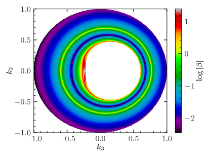
Figure 6: The dispersive GSHE-to-geodesic delay parameter $\beta$ as a function of the maximum $\epsilon=0.01$ initial momentum parameterized by $k_{2}$ and $k_{3}$ (Eq. 2.15). The source is placed at $(5\,R_{\rm s},\pi/2,0)$ and the “observer” is defined as the point where the $\epsilon_{max}$ trajectory intersects a sphere of radius $50\,R_{\rm s}$. Each pixel represents an $\epsilon$ bundle of trajectories.

Figure 7: The geodesic magnification $\mu_{\rm GO}$ as a function of the initial emission direction $(k_{2},k_{3})$, corresponding to the $\beta$ calculation of Fig. 7. The source is placed at $(5\,R_{\rm s},\pi/2,0)$. The outer green ring of Fig. 7 is magnified (red ring), while trajectories passing close to the BH shadow are demagnified.

III.1.3 Directional dependence of the GSHE

We now report on the directional dependence of the time delay from the source point of view, considering trajectories that initially point towards the BH. We emit a GSHE trajectory from the source at the maximum value of $\epsilon$ in the direction parameterized by $(k_{2},k_{3})$, introduced in Eq. 2.15. Then we record the angular coordinates where this trajectory intersects a far origin-centered sphere of radius $50\,R_{\rm s}$, setting that location as the “observer” for the above choice of initial direction. We find the remaining GSHE and geodesic trajectories that connect to the same point and form a bundle of trajectories. Starting with the maximum value of $\epsilon$ guarantees that we never fix an observer in the blind spot of any GSHE trajectories.

We characterize each bundle belonging to an initial choice of $(k_{2},k_{3})$ by $\beta$ of the right-polarized rays in the left panel of Fig. 7 (note that the directions in this figure correspond to the initial directions of the GSHE rays with maximum $\epsilon=0.01$). Throughout, we keep the source at $(5\,R_{\rm s},\pi/2,0)$ and do not calculate the left-polarized rays, as those behave sufficiently similarly. This time, we do not eliminate the initial directions that result in trajectories that completely loop around the BH. We still have $\alpha\approx 2$, although a small fraction of the initial directions, particularly close to the BH horizon, deviate by $\sim 1\%$. The left panel of Fig. 7 shows a characteristic ring of initial directions that produce $|\beta|\sim 1$, which approximately corresponds to the trajectories that are mapped to the point opposite side of the BH (more precisely, these trajectories are mapped close to the edge of the blind spot for the maximum $\epsilon=0.01$). The initial directions close to the BH horizon produce $|\beta|\sim 10$, although these are extreme configurations that completely loop around the BH and are demagnified. The initial directions of the outgoing trajectories (not shown in Fig. 7) result in $|\beta|$ lower than the minimum of the ingoing trajectories and therefore are of little interest for the detection of the GSHE.

Having demonstrated how $|\beta|$ depends on the direction of the emission, we now study the dependence of the corresponding magnification factor. We again verify that the deviation of the magnification as a function of $\epsilon$ from its geodesic is at most $\sim 1\%$, although typically smaller by up to several orders of magnitude. In Fig. 7, we show $\mu_{\rm GO}$ as a function of the emission direction, matching Fig. 7. Additionally, in Fig. 9 we explicitly show a scatter plot of $\mu_{\rm GO}$ and $\beta$ corresponding to the pixels in Fig. 7 and Fig. 7. The scatter plot displays two high $|\beta|$ tails – one where $|\beta|$ is positively correlated with $\mu_{\rm GO}$ and one where the correlation is negative. The former corresponds to the aforementioned outer green ring of Fig. 7 of bundles that approximately reach the point on the other side of the BH and are magnified as they converge into a smaller region. The latter is demagnified, as it consists of bundles that pass close to the BH horizon and are sensitive to the initial direction. Therefore, it is the outer green ring of Fig. 7 that comprises a promising landscape for observing the GSHE due to its high $|\beta|$ and $|\mu_{\rm GO}|>1$.

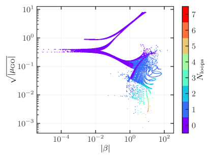
Figure 8: The relation between the geodesic magnification $\mu_{\rm GO}$ and $|\beta|$ in pixels of Fig. 7. The colour represents the number of complete loops $N_{\rm loops}$ around the BH. The magnified region in the top right consists of the high $|\beta|$ outer green ring in Fig. 7. The demagnified region in the bottom right consists of bundles that pass very close to the BH horizon.

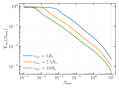
Figure 9: Fraction of the source celestial half-sphere that yields $|\beta|\geq\beta_{\min}$. In the region where $\Upsilon$ is decaying we approximately have $\Upsilon\propto 1/r_{\rm src}^{2}$. The source is in the equatorial plane and $a=0.99$. The $r_{\rm src}=5\,R_{\rm s}$ line corresponds to Fig. 7.

We calculate the fraction of the source celestial half-sphere of Fig. 7 that yields $|\beta|>\beta_{\rm min}$ of the GSHE-to-geodesic delay for the right-polarized rays as

$$\Upsilon_{\rm src}(\beta_{\min})=\frac{1}{2\pi}\int H(|\beta|-\beta_{\min})\sin\psi\differential\psi\differential\rho,$$ (3.5)

where the integral runs over the celestial half-sphere of ingoing trajectories, $H(\cdot)$ is the Heaviside step function defined as $H(x)=1$ if $x>0$ and $0$ otherwise. We note that a fraction of the half-sphere is covered by the shadow of the BH and, therefore, $\Upsilon_{\rm src}(0)<1$. We plot $\Upsilon_{\rm src}(\beta_{\min})$ in Fig. 9 for sources at $(r_{\rm src},\pi/2,0)$, where we choose $r_{\rm src}=5,7.5,10\,R_{\rm s}$ and $a=0.99$. We find that for $r_{\rm src}=5\,R_{\rm s}$ about $5\%$ of the ingoing half-sphere yield $|\beta|\gtrsim 0.5$, and we verify that $\Upsilon_{\rm src}$ is approximately proportional to $1/r_{\rm src}^{2}$ in the region where it is decaying.

Similarly, we calculate the fraction of the far sphere of radius $r=r_{\rm obs}$ where an observer would measure $|\beta|>\beta_{\rm min}$ and $\mu>|\mu_{\rm min}|$:

$$\begin{split}\Upsilon_{\rm obs}(\beta_{\min},\mu_{\min})=&\frac{1}{4\pi}\int\mathcal{S}(\beta,\mu)\sin\phi\differential\phi\differential\theta,\\ =&\frac{1}{4\pi}\int\mathcal{S}(\beta,\mu)\frac{\sin\psi}{|\mu(\psi,\rho)|}\differential\psi\differential\rho.\end{split}$$ (3.6)

Here, $(\theta,\phi)$ are coordinates on the spacetime sphere $r=r_{\rm obs}$, and $(\rho,\psi)$ are coordinates on the celestial sphere of the source. The Jacobian relating both coordinates is the inverse of the magnification, as has been included in the second line: this can be intuitively understood as magnified/demagnified trajectories being focused/spread out and therefore less/more likely. The integral is weighted by a selection function

$$\mathcal{S}=H(|\beta(\phi,\theta)|-\beta_{\min})H(|\mu(\phi,\theta)|-\mu_{\min}),$$ (3.7)

eliminating trajectories that are either too faint to be detected or for which the GSHE is undetectable. We are considering trajectories that loop around the BH. Therefore, multiple trajectories can reach an observer, so $\Upsilon_{\rm obs}>1$ in general when computing probabilities (Section IV.5).

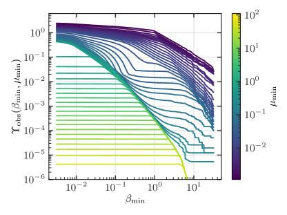
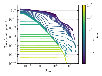
Figure 10: Observer’s cumulative GSHE probability as a function of the minimum magnification (absolute value), including all trajectories (left) and excluding trajectories that loop around the BH (right). Only trajectories with $|\mu|>10^{-3}$ are considered. Differences are appreciable only for $\mu\ll 1$.

Fig. 10 shows the observer’s cumulative GSHE probability for different magnification cuts. Two cases are considered: the left panel allowing for any number of loops around the BH, which has a maximum number of $7$ in our numerical exploration. The right panel restrict the results to zero loops, although strongly deflected trajectories with $\alpha<2\pi$ are still considered (these trajectories could be discriminated by the sign of $\mu$, as they have negative parity). The differences are noticeable only for faint trajectories with $|\mu|\ll 1$: for $\beta_{\min}\lesssim 1$ $\Upsilon_{\rm obs}$ is larger than unity, reflecting the existence of these additional trajectories. For $\beta_{\min}\gtrsim 1$ the additional loops increase the probability considerably. Note that the high $\beta$ end is restricted by the resolution in our numerical exploration.

The results can be adapted to different distances between the source and the BH without an additional sampling. The GSHE probability for the source scales as $\Upsilon_{\rm src}\propto r_{\rm src}^{-2}$, cf. Fig. 9, as the regions contributing to the different values of $\beta$ span a smaller portion of the source’s sphere. Additionally, the magnification scales by the same factor $\mu\propto r_{\rm src}^{-2}$ [59], reflecting the divergence of rays before encountering the lens.

Lastly, in Appendix C we discuss the relation between the image parity of trajectory bundles of Fig. 7 and the sign of the GSHE-to-geodesic delay. Appendix D discusses the effect of multiple loops and sign of $\beta$ on the observer’s probability.

III.1.4 Dependence on the remaining parameters

We postpone the discussion of varying the BH spin $a$ and the azimuthal angle of the observer $\phi_{\rm obs}$ to Appendix B. However, we highlight that in the Schwarzschild metric, the right-to-left delay vanishes because of reflection symmetry. On the other hand, the GSHE-to-geodesic delay is maximized in Schwarzschild, which we attribute to the fact that lowering the BH spin pushes its horizon outwards, and therefore the trajectories pass closer to the BH horizon where the gradient of the gravitational field is larger. We verify that this behavior is not a consequence of a particular source-observer configuration and qualitatively holds in general.

III.2 Waveform comparison

We consider the IMRPhenomXP waveform [101] of a $50$ and $35M_{\odot}$ binary BH merger observed at an inclination angle of $0.9\pi$ with the spin of the primary along the $z$-axis $a_{z}=0.7$ and $0$ along the remaining axes and zero spin of the secondary. The frequency-domain waveform is generated from $40\leavevmode\nobreak\ \mathrm{Hz}$ to $1024\leavevmode\nobreak\ \mathrm{Hz}$, though the merger frequency is $\sim 225\leavevmode\nobreak\ \mathrm{Hz}$. Following Eq. 2.7, we fix the background mass to achieve some maximum value $\epsilon_{\max}$ at the lower frequency limit, since $\epsilon\propto 1/f$.

As an example, for $\epsilon_{\max}=0.1$ this amounts to $M\sim 5\times 10^{4}\leavevmode\nobreak\ M_{\odot}$. Following Eq. 3.2, the GSHE-to-geodesic and right-to-left observer time delays are

$$\Delta\tau(f) \approx 3\leavevmode\nobreak\ \mathrm{ms}\,\beta\left(\frac{5\times 10^{4}M_{\odot}}{M}\right)\left(\frac{40\leavevmode\nobreak\ \mathrm{Hz}}{f}\right)^{2},$$ (3.8a)

$$\Delta\tau_{\rm R-L}(f) \approx 0.3\leavevmode\nobreak\ \mathrm{ms}\,\beta_{\rm R-L}\left(\frac{5\times 10^{4}M_{\odot}}{M}\right)^{2}\left(\frac{40\leavevmode\nobreak\ \mathrm{Hz}}{f}\right)^{3}.$$ (3.8b)

The GSHE-to-geodesic delay is the dominant component. Moreover, typically $|\beta|\gg|\beta_{\rm R-L}|$ as demonstrated in Section III.1. The GSHE-to-geodesic delay shifts both polarizations in approximately the same direction with respect to the geodesic, as exemplified in Figure 3. Their difference is the right-to-left delay, which is negligible in most cases. Therefore, we will focus on the difference between the GSHE-corrected and geodesic-only waveforms.

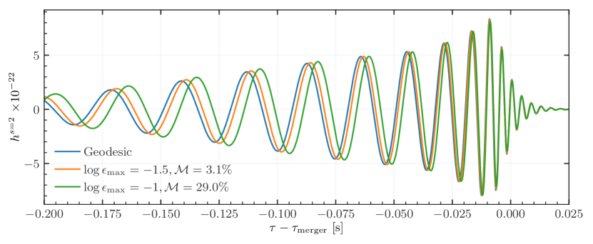
Figure 11: The GSHE-corrected and geodesic-only right polarization waveforms of a $50$ and $35M_{\odot}$ merger if $\beta=2$. We show two cases of $\epsilon_{\rm max}$, the perturbation strength at the lower frequency range of the waveform, along with the corresponding GSHE-induced mismatch. The GSHE manifests as a frequency-dependent phase shift in the inspiral part of the signal.

In Fig. 11, we compare the right-polarization geodesic-only and GSHE-corrected waveforms for $\beta=2$ separately if $\log\epsilon_{\max}=-1.5,-1$. This choice of $\beta$ is large enough to demonstrate the GSHE, but still reasonably likely, as we showed in Fig. 7 and Fig. 9. We follow the modeling prescription of Eq. 2.24. Even in the former, more conservative $\epsilon_{\max}$ case, the effect on the waveform is clearly visible and manifested as a frequency-dependent phase shift in the inspiral phase of the merger. This is because the merger and the ringdown are propagated by higher frequency components whose GSHE correction is suppressed as $\sim 1/f^{2}$. Consequently, the intrinsic parameters inferred from the inspiral part of the waveform may appear inconsistent with the merger and ringdown part of the waveform if the GSHE is not taken into account. We do not explicitly show the detector strain, which is a linear combination of the right- and left-polarization state waveforms whose phase difference due to the GSHE is negligible.

In Fig. 12 we plot the mismatch of the right-polarization waveform calculated following Eq. 2.30. We assume that in $\Delta\tau$ the exponent is $\alpha=2$. We show the mismatch for several choices of $\epsilon_{\max}$, which is equivalent to scaling the background mass $M$ while keeping the waveform fixed. Following Eq. 2.32, this shows that we can approximate the mismatch as $\mathcal{M}\propto\beta^{2}$ for small mixing angles $\gamma$.

IV Discussion

In the derivation of the GSHE and throughout this work, several simplifying assumptions have been made to demonstrate the viability of this effect for future detection. We now first comment on the neglected higher-order contributions to the GSHE in Section IV.1, the source-observer placement in Section IV.2 and the GW emission anisotropy in Section IV.3. Then, in Section IV.5 we discuss the prospects of detecting the GSHE and, finally, in Section IV.4 we discuss its relation to tests of GR and beyond-GR theories.

IV.1 Higher-order GSHE contributions

The GSHE equations describe the motion of a wave packet energy centroid and are only valid up to first order in wavelength. The relevant indicator is the WKB perturbation parameter $\epsilon$, the ratio between the wave packet wavelength and the BH Schwarzschild radius. In the limit of $\epsilon\rightarrow 0$ the geodesic propagation of the wave packet is recovered, while $\epsilon\sim 1$ is the regime of wave-like phenomena, wherein the wavelength is comparable to the characteristic length scale of the system. Going further, if $\epsilon\rightarrow\infty$ we do not expect wave propagation to be significantly affected by the presence of the BH as in this limit the presence of the BH becomes negligible (see, for example, Ref. [102, Fig. 2]).

The terms of order $\epsilon^{2}$ and higher were neglected in the derivation of the GSHE. In this work, we use a maximum value of $\epsilon=0.1$, at which point we assume that the beyond-linear terms are still negligible. Nevertheless, in Fig. 12 we showed that the effect is significant even when this maximum $\epsilon$ is relaxed. The neglected higher-order contributions are likely to induce wave-like phenomena, such as diffraction, as we depart further from the regime of GO. However, the GSHE treatment describes the motion of the energy centroid of a wave packet, which is only well defined if $\epsilon\ll 1$. When the wavelength reaches $\epsilon\sim 1$ the WKB expansion up to an arbitrary order in $\epsilon$ becomes of little interest, as the perturbation series in $\epsilon$ inevitably breaks down. Therefore, instead of extending the WKB analysis to higher orders, it is potentially more instructive to directly solve the linearized gravity perturbation propagation via, e.g., the Teukolsky equation approach [103, 102, 104]. This approach was used to study GW emission in hierarchical triple systems in Ref. [105]. An alternative but no simpler route would be a path integral approach of summing over all possible paths connecting the source and observer, whose extremum would be the classical trajectories considered in this work  [106]. The upside of the former treatment is its validity up to an arbitrary $\epsilon$. Moreover, it would allow matching the GSHE results in an appropriate limit.

IV.2 Source and observer placement

We assumed that both the observer and the source are static. The assumption of a static, far observer in the Kerr metric is a good approximation if we consider $r_{\rm obs}\rightarrow\infty$, as would be the case for astrophysical observations. Throughout this work, we ensured that our conclusions are independent of the distance of the observer from the BH. Additionally, one needs to consider the gravitational and cosmological redshift. We verified that the gravitational redshift due to escaping the strong-field regime of the background BH has a negligible dependence on $\epsilon$. It affects both the geodesic and GSHE rays equally, and we do not consider it further. The cosmological redshift due to the expansion of the universe is independent of the frequency and, thus, enters as a simple multiplicative factor.

On the other hand, the assumption of a static source may break down, particularly if the source is as close to the BH as we have considered above. This depends on the distance traveled by the source while the signal is emitted over the frequency range of a given detector. The former factor depends on the orbital period of the binary around the background BH

$$T_{\rm orb}\approx 138\,s\left(\frac{\mathcal{A}}{10\,R_{\rm s}}\right)^{3/2}\left(\frac{M}{5\times 10^{4}M_{\odot}}\right),$$ (4.1)

where $\mathcal{A}$ is the semi-major axis of the orbit. The in-band duration of the signal depends on the GW source masses and intrinsic parameters. The typical range of LVK in-band source duration are $0.1-100\leavevmode\nobreak\ \mathrm{s}$. The static-source assumption limits the validity of our results to shorter in-band events, including the more massive mergers expected in dynamical formation scenarios and AGN. Our framework can be applied to longer events (e.g. lighter sources such as binary neutron star mergers), but only if they orbit a sufficiently massive BH, or are located sufficiently far. Source motion also needs to be accounted for if the GSHE signature is very sensitive on the source position. This can happen in strongly aligned systems, or for trajectories that undergo a very strong deflection, such as multiple loops around the BH.

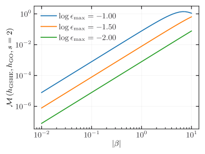
Figure 12: The percentage mismatch $\mathcal{M}$ of the GSHE-induced corrections as a function of $|\beta|$ for several choices of the maximum perturbation strength $\epsilon_{\rm max}$ and the waveform of Fig. 11.

The static source assumption will be severely violated by stellar mass black holes emitting in the LISA frequency band. These sources have wavelengths several orders of magnitude larger than LVK sources. They evolve very slowly in frequency and can be observed over several years [71, 72], completing multiple orbits around the massive BH [58]. A treatment of a moving source would require the composition of the GSHE signal across multiple time steps and accounting for the Doppler effects; see Refs. [74, 76]. While the very low frequency ($\sim\mathrm{mHz}$) enhances the GSHE corrections, the slow frequency evolution might make a detection challenging. Moreover, at such low frequencies the perturbative expansion in $\epsilon$ may break down, necessitating a treatment in the wave optics regime, unless the background BH is sufficiently massive as described in Eq. 2.7.

Another potential issue is whether the binary is tidally disrupted by the background BH. This can be described by the Hills mechanism [107, 108, 109] and a significant perturbation occurs when the tidal force induced by the background BH is of the same order as the binary’s self-gravity. This effect has been estimated in Ref. [105] for hierarchical triple systems similar to the ones we are considering. For a binary with an orbital period of $1/f$, tidal effects become important when the binary is at a radius

$$r_{t}\lesssim\frac{2M}{(Mf)^{2/3}}=2M\epsilon^{2/3}.$$ (4.2)

In this paper, we always consider GW with wavelengths smaller than $\epsilon_{\rm max}=0.1$. Thus, tidal effects can be safely ignored, as they only become significant if the binary is placed at the radius of $r_{t}\lesssim 0.43M$, which is below the event horizon of the background BH. Thus, binary disruption only affects our results indirectly, by precluding the formation of binaries with $\epsilon\gg 1$, which may later evolve to the range of frequencies probed by LVK. Addressing this effect requires detailed considerations on dynamical binary formation and migration beyond the scope of this work.

IV.3 Emitter anisotropy

We have considered an isotropic GW emitter. However, a binary merger is an anisotropic emitter – similar to an electric dipole – and the emitted power has a directional dependence (see Ref. [59] for a treatment of strong-field lensing by Schwarzschild BH). There are two effects in which the angular dependence of the source might play a role. First, for a given $\epsilon s$-dependent set of trajectories connecting the source and observer, the initial emission direction must be rotated away from the geodesic emission direction by an angle that is approximately proportional to $\epsilon$. This generally corresponds to an angle of $\sim 1\leavevmode\nobreak\ \mathrm{degrees}$ or lower between the low- and high-frequency components of the signal. This value is well below the sensitivity to the GW intrinsic parameters, such as the orbital inclination $\iota$.

Second, the angular structure of the source can cause substantial differences in the multiple images (bundles) caused by the background BH. The multiple images may have different relative amplitude, polarization, and merger phase, depending on which angular portion of the binary is projected onto the source for each trajectory. As an example, consider the configuration shown in Fig. 2, in which the two bundles depart in opposite directions from the source. In contrast, each GSHE trajectory encompasses an angular deviation proportional to $\epsilon$ relative to the geodesic limit for that bundle. This difference is unrelated to the GSHE corrections. However, further studies quantifying the detectability of the GSHE will need to explore this effect.

IV.4 Relation to tests of GR

If not accounted for, the GSHE might be incorrectly interpreted as a deviation from GR. In contrast, a detection favoring beyond GR physics has to be distinguished from the GSHE. Due to its frequency dependence, the GSHE mimics three tests of GR: a modified dispersion relation, constraints of the post-Newtonian parameters, and consistency of the inspiral, merger, and ringdown phases of the signal. We will focus on the modified dispersion relation, which exactly mimics the GSHE-to-geodesic time delay (i.e. $\beta$) if the right-to-left delay is negligible. The connection to the other tests is not straightforward. Hence, we will focus on the modified propagation, Eq. 4.3.

The GSHE-induced delay is degenerate with a modified dispersion relation of the form

$$E^{2}=p^{2}+c_{0},$$ (4.3)

in the limit $|c_{0}/(hf)^{2}|\ll 1$, where $h$ is Planck’s constant. This is a particular case of a generic violation of Lorentz invariance, in which a term proportional to $p^{n}$ is added  [110, 111, 112]. Our case ($n=0$) is equivalent to a graviton mass $m_{g}^{2}=c_{0}>0$ if the correction has a positive sign. However, the GSHE time delay can have either sign depending on the configuration. A modified dispersion causes a frequency-dependent time delay of a GW signal

$$\Delta\tau_{c_{0}}=\frac{c_{0}D}{(hf)^{2}}+\mathcal{O}\left(\frac{c_{0}^{2}}{h^{4}f^{4}}\right),$$ (4.4)

where $D$ is an effective distance to the source that coincides with the standard luminosity distance for low redshift sources [81, Eq. 56] (see also Ref. [113]).

Equating Eq. 4.4 and Eq. 3.2 yields a relation between the GW propagation and GSHE parameter

$$\beta\approx\frac{G}{c^{4}h^{2}}MDc_{0}\approx 0.148\frac{M}{5\times 10^{4}M_{\odot}}\frac{D}{\text{Gpc}}\frac{c_{0}}{(10^{-23}\text{eV})^{2}},$$ (4.5)

The GSHE-induced delay coefficient can be probed up to a factor $\propto MD$. The effective distance $D$ is related to the source’s distance (see Ref. [110, Eq. 5]), which is constrained by the amplitude of the signal. In contrast, the mass $M$ of the background BH is unknown a-priori. Measuring $M$ would be possible if multiple signals are received, e.g. by measuring their time delay and magnification ratio. For a single signal, it might be possible to constrain $M$ from the orbital acceleration of the binary around the background BH, cf. Eq. 4.1. Other means of constraining $M$ may include identifying the source’s environment, e.g. via an electromagnetic counterpart, or statistically, e.g. modeling the distribution of mergers around massive BH.

Event	$D_{\rm L}\left[\mathrm{Mpc}\right]$	$M_{\rm tot}\left[M_{\odot}\right]$	$\beta_{+}$	$\beta_{-}$
GW190706	$5400$	$190$	$1.35\times 10^{0}$	$1.2\times 10^{-1}$
GW190707	$780$	$23$	$1.5\times 10^{-1}$	$7.5\times 10^{0}$
GW190708	$890$	$36$	$1.85\times 10^{-1}$	$8.5\times 10^{-1}$
GW190720	$770$	$25$	$3.3\times 10^{-1}$	$3.4\times 10^{-1}$
GW190727	$3000$	$110$	$1.75\times 10^{-1}$	$2.1\times 10^{-1}$
GW190728	$920$	$24$	$3.9\times 10^{-1}$	$2.4\times 10^{-1}$
GW190814	$300$	$27$	$1.3\times 10^{-1}$	$5.0\times 10^{-2}$
GW190828	$2200$	$80$	$7.5\times 10^{-2}$	$4.7\times 10^{-1}$
GW190910	$1900$	$100$	$4.65\times 10^{-2}$	$3.75\times 10^{-1}$
GW190915	$1700$	$77$	$8.5\times 10^{-2}$	$4.3\times 10^{-1}$
GW190924	$580$	$16$	$6.0\times 10^{0}$	$1.85\times 10^{-1}$
GW191129	$800$	$20$	$6.0\times 10^{-1}$	$4.95\times 10^{-1}$
GW191204	$600$	$23$	$1.6\times 10^{-1}$	$5.0\times 10^{-2}$
GW191215	$1900$	$58$	$7.0\times 10^{-2}$	$4.05\times 10^{-1}$
GW191216	$360$	$21$	$1.5\times 10^{0}$	$6.0\times 10^{-2}$
GW191222	$3100$	$120$	$7.0\times 10^{-2}$	$4.4\times 10^{-1}$
GW200129	$870$	$76$	$5.5\times 10^{-1}$	$4.6\times 10^{-2}$
GW200208	$2300$	$92$	$8.0\times 10^{-2}$	$1.9\times 10^{-1}$
GW200219	$3700$	$100$	$7.0\times 10^{-2}$	$4.0\times 10^{0}$
GW200224	$1700$	$95$	$8.0\times 10^{-2}$	$1.85\times 10^{-1}$
GW200225	$1100$	$41$	$8.5\times 10^{-2}$	$1.7\times 10^{1}$
GW200311	$1100$	$75$	$6.0\times 10^{-2}$	$1.85\times 10^{-1}$

Table 1: 90% c.l. limits on $\beta$ from LVK tests of Eq. 4.3, separately for positive and negative values of $c_{0}$ while assuming background BH mass of $5\times 10^{4}$. We also show the median total mass $M_{\rm tot}$ and luminosity distance $D_{\rm L}$.

The relation in Eq. 4.5 allows us to convert LVK tests of Eq. 4.3 into constraints on $\beta/M$. We use the full posteriors samples from the events analyzed in the third observation run [111, 112]. The results are shown in Table 1, where he show the $90\%$ c.l. (confidence level) for positive and negative values of $c_{0}$, assuming a fiducial mass of $5\times 10^{4}M_{\odot}$. We note that the LVK analyses employ a weakly informative prior on $\log(c_{0})$, extending many orders of magnitude below the range where the data can probe Eq. 4.3. Therefore, most of the posterior samples lie in a region that is indistinguishable from GR, leading to poor sampling of the region where data is informative. An analysis with non-logarithmic priors would lead to more efficient sampling and avoid the need to treat positive and negative values of $\beta/c_{0}$ separately.

The key difference between a modified dispersion relation of Eq. 4.3 and the GSHE is that the former is universal: the same coefficient $c_{0}$ represents a fundamental property of gravity and modifies the waveforms of all GW events. On the contrary, the GSHE is environmental and the correction is expected to vary between events. Therefore, to constrain $\beta$ from LVK bounds on anomalous GW propagation, it is necessary to use the bounds on $c_{0}$ for individual events, rather than the combined value quoted by LVK [110, 111, 112]. Another consequence is that GW propagation tests depend on the source distance, while the GSHE does not. Therefore, the $D-c_{0}$ correlations need to be taken into account when using Eq. 4.5 to constrain $\beta$, e.g. using the full posteriors (as in Table 1).

We note that the birefringent GSHE (i.e., polarization-dependent time of arrival due to $\beta_{\rm R-L}$) resembles other beyond-GR effects discussed in the literature. Scalar-tensor theories with derivative couplings to curvature [114] predict that different GW (and additional) polarization states travel at different speeds on an inhomogeneous spacetime. This birefringent effect is different from ours in three respects [82]: 1) it involves a difference in the $+/\times$ polarization, rather than R-L (right-to-left), 2) it is independent of frequency, and 3) it depends on the curvature of beyond-GR fields, which can be important over astronomical scales, rather than being confined to the vicinity of a compact object. Therefore, the time delay between polarization states associated to these theories is not bounded to any specific scale, and can range from negligible to astronomical, depending on the theory and the lensing configuration. The lack of observation of birefringence in LVK data sets stringent bounds on alternative theories [115]. As deviations from GR become stronger near a compact object, detecting the GSHE imprints for mergers near a massive black hole would set extremely tight bounds on such theories.

Finally, another beyond-GR birefringence effect has been studied in Ref. [83] as emerging from higher-order corrections to GR [116, 117]. Like the GSHE, this form of GW birefringence involves the circular polarization states and depends on frequency, although it grows with $f$ rather than decaying like the GSHE. Moreover, it is again assumed to be a universal property of gravity, rather than an environmental, event-dependent effect. The analysis in Ref. [83] showed that all but two GW events analyzed were compatible with GR. The outliers, GW190521 and GW191109, preferred their form of birefringence over the GR prediction. However, one cannot easily interpret this preference as due to the GSHE, as a significant $\beta_{\rm R-L}$ is unlikely and an analogue of our, typically larger, GSHE-to-geodesic delay due to $\beta$, has not been included in the analysis. Unfortunately, LIGO-Virgo did not quote any results on $c_{0}$ (Eq. 4.4) for that event. Therefore, a more detailed analysis would be required before reaching any conclusions.

IV.5 Detection prospects and applications

Throughout this work we considered GW sources very close to the background BH to illustrate the consequences of the GSHE on a waveform. We have focused on the case of a background BH in the range of intermediate-mass to massive of $\sim 10^{5}M_{\odot}$. This results in reasonable values of $\epsilon$ that make the GSHE detectable for terrestrial observatories. In case of studying the detectability of the GSHE with the longer wavelength LISA-like signals, the background BH mass would have to be correspondingly increased to achieve similar values of $\epsilon$, such as super-massive BH. We expect that there will be a partial degeneracy between the delay proportionality factor $\beta$ and the ratio between the wavelength and the background BH mass, as both control the strength of the GSHE corrections. Nevertheless, by their definition $\beta$ is independent of frequency, and therefore sufficiently high-quality data should break this degeneracy.

One of the environments to produce promising signals are AGN, whose potential is discussed, e.g., in Ref. [118]. BH (and binaries thereof) are expected to migrate radially inward and form the so-called binary-single interactions [119]. This radial migration may bring the BH as close as $\sim 6\,R_{\rm s}$ to the background BH [56]. Furthermore, migration traps could promote the growth of intermediate-mass BH around AGN [120]. In addition, a population of intermediate-mass BH is expected in globular clusters, although no clear detection is available as of today to constrain their population [121]. We consider AGN and globular clusters to be the most likely candidates to host the hierarchical triple systems we consider, although their respective binary BH populations also remain poorly constrained [122]. Although we have focused mainly on BH mergers, neutron star binaries in close proximity to an AGN would be ideal to probe the GSHE, in addition to nuclear physics [123].

We find there to exist at least two favorable source-observer configurations that result in a strong GSHE: aligned and close-by setups. The aligned setup occurs when the source and observer are approximately on opposite sides of the background BH. We show in Fig. 7 that in this case there exists a ring of initial directions that results in $|\beta|\gtrsim 1$. Because such trajectories converge to a small region opposite the source, they are also magnified, which is represented by the high $|\beta|$ and high magnification cluster of points on Fig. 9. Additionally, we demonstrate that in this case it is not necessary for the source to be within a few $R_{\rm s}$ of the background BH. The sufficient condition is for the trajectories to pass close to the BH. In Fig. 9, we show that the fraction of these initial directions falls approximately as $1/r_{\rm src}^{2}$. This is likely to be at least partially balanced by the fact that more mergers may occur from the outer regions of the AGN or globular cluster.

The close-by setup occurs for generic source-observer placements, but requires proximity between the source and the background BH. Even if the source, BH and the observer are not aligned, there is always a strongly deflected connecting bundle that propagates very close to the background BH and thus undergoes significant GSHE corrections. In Fig. 5, we showed that the delay proportionality factor $\beta$ of such bundles tends to a constant, non-negligible value even for large separations between the source and the background BH. These trajectories exist in general, but their detectability is limited by demagnification, which is significant for sources far from the background BH and/or large deflection angles. Hence, in this setup we expect the GSHE to be detectable only for sufficiently close sources, although for most observer locations.

Our scenario predicts the reception of multiple GW signals, associated with each of the bundles connecting the source and the observer. The time delay between the signals (bundles) is proportional to the mass of the background BH, and together with the relative magnification carries information about the geometry of the system. Furthermore, each image will contain GSHE corrections of different strengths. In the aligned setup, we expect the two magnified images to have only a short time delay between them. The GSHE corrections have a sizeable $\beta$, but generally each has an opposite sign, as exemplified in Fig. 3. In the close-by setup, we expect to first detect a signal with $\beta\ll 1,\,|\mu|\approx 1$, followed by a demagnified one with a strong GSHE (large $|\beta|$, $|\mu|\ll 1$). Unless the source is very close to the background BH, the second image will likely appear as a sub-threshold trigger due to exponential demagnification.

The tools developed for the search and identification of strongly lensed GW  [124, 125] can be applied to searches for GSHE imprints. A possible approach to find strongly lensed GW events is to use the posterior distribution of one image as a prior for the other image, since the two should agree if they describe the same merger [126]. The short time delays between signals involved in our scenario offer two advantages. First, by lowering the chance of an unrelated event being confused as another image [127] and, secondly, by narrowing down the interval within which to search for sub-threshold triggers carrying a GSHE imprint. If the signal contains higher modes, it may be possible to distinguish type II images (saddle points in the lensing potential) from type I/III (local minima/maxima) due to the lensing-induced phase shift [128, 129, 130]. This would provide another handle on the lensing setup, as the secondary image (negative parity, lower $\mu$) carries this phase.

Exp.	$M\,[M_{\odot}]$	$V_{\mathcal{G}}\,[{\rm Gpc}^{3}]$	$z_{\mathcal{G}}$	$\mathcal{R}^{10{\rm yr}}_{90}\,[{\rm Gpc}^{-3}{\rm yr}^{-1}]$
LIGO	$10^{4}$	$0.10$	$0.06$	$2.41$
	$10^{5}$	$0.01$	$0.03$	$22.92$
	$10^{6}$	$0.25\times 10^{-3}$	$0.70\times 10^{-2}$	$9.04\times 10^{2}$
	$10^{7}$	$0.24\times 10^{-6}$	$0.67\times 10^{-5}$	$9.47\times 10^{5}$
CE	$10^{4}$	$18.58$	$0.41$	$0.01$
	$10^{5}$	$2.40$	$0.20$	$0.10$
	$10^{6}$	$0.37$	$0.10$	$0.62$
	$10^{7}$	$0.28\times 10^{-2}$	$0.02$	$82.36$
ET	$10^{4}$	$30.42$	$0.50$	$0.76\times 10^{-2}$
	$10^{5}$	$3.41$	$0.22$	$0.07$
	$10^{6}$	$0.52$	$0.12$	$0.44$
	$10^{7}$	$0.02$	$0.04$	$13.68$

Table 2: Effective detection volume and equivalent redshift for different detectors and background BH masses. The results assume a $30+30M_{\odot}$ source at a distance of $r_{\rm src}=5\leavevmode\nobreak\ R_{\rm s}$ from the BH, with a detection threshold of $\rho_{\rm thr}=8$. The last column displays the 10-yr 90% c.l. limits on the merger rate for events with this characteristic, assuming no observation (in units of ${\rm Gpc}^{-3}{\rm yr}^{-1}$).

The GSHE could be used to investigate the environment of GW sources. The time delay between signals associated with different bundles can be used to constrain the background BH mass $M$, and $\beta$ can be used to infer the alignment of the source and observer and, potentially, the background BH spin. Furthermore, a detection of a nonzero $\beta_{\rm R-L}$ would further indicate a nonzero BH spin. In addition, the source’s peculiar acceleration may be used to recover information on the mass of the background BH if the static-source approximation is broken, cf. Eq. 4.1. If the acceleration can be considered constant, it will impart a $\propto f^{2}$ correction to the phase, which can be distinguished from the GSHE. If the deviation from the static source approximation is dramatic, as expected for LISA stellar-mass sources, much more information about the orbit can be recovered, e.g. [76].

The capacity to detect GSHE corrections in GW catalogs remains largely dependent on astrophysical factors. In this exploratory work, we demonstrate that there exist plausible configurations in which the GSHE is significant. A detectability study of the GSHE would strongly depend on the prior knowledge of the background BH population, the merger rates in their environments and their location relative to the background BH. We show that the GSHE-induced mismatch can reach $\mathcal{M}\sim 10\%$. Under the mismatch and SNR criterion that two waveforms are distinguishable if the product $\mathcal{M}\times\text{{SNR}}^{2}\gtrsim 1$ [131], we expect LVK detectors to find GSHE signatures if enough stellar-mass binaries merge in the vicinity of background BH of intermediate mass. Recent studies of lensed gamma-ray bursts point towards a population of objects with $M\sim 10^{4}M_{\odot}$ [132, 133, 134], an ideal mass range to observe the GSHE.

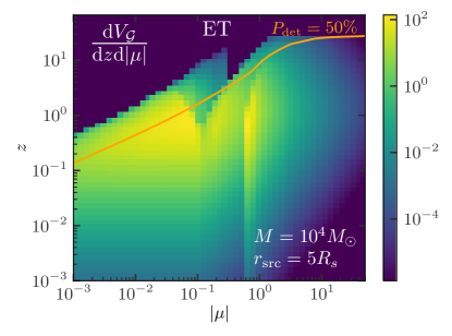
Figure 13: Differential effective volume, Eq. 4.6 as a function of the magnification and redshift. The plot applies to a $30+30M_{\odot}$ binary at $5\leavevmode\nobreak\ R_{\rm s}$ of a $10^{4}M_{\odot}$ background BH, observed by the Einstein Telescope (see text). The solid line shows the median response distance.

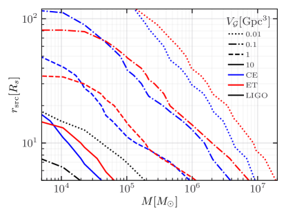
Figure 14: Effective volume Eq. 4.6 as a function of the background BH mass and the separation of the source. Lines show contours of equal $V_{\mathcal{G}}$ for different detectors.

We now estimate the prospects of GW detectors to distinguish the GSHE in a signal. To simplify the analysis, we focus on a $30+30M_{\odot}$, non-spinning, quasi-circular binary merging at a distance of $r_{\rm src}=5\leavevmode\nobreak\ R_{\rm s}$ from a $10^{4}M_{\odot}$ BH. We use the IMRPhenomD waveform model [135], our framework and code for detection probabilities are based on Ref. [136]. We consider two setups using the LIGO (O4 curve in Ref. [137]), CE (CE; [138]) and ET (ET; [139]) noise curves. We assume a single interferometer for simplicity: prospects will improve when considering the LVK network, multiple arm combinations in ET or a next-generation network of ground detectors [140] thanks to improved SNR and sky coverage.

We quantify the observational prospects by defining the effective observable volume as

$$V_{\mathcal{G}}=\int\differential z\frac{\differential V_{z}}{\differential z}(z)\int\differential|\mu|P_{\rm det}\frac{\differential\Upsilon_{\rm obs}}{\differential|\mu|}.$$ (4.6)

Here, $\frac{\differential V_{z}}{\differential z}(z)$ is the comoving volume element at the source’s redshift and $P_{\rm det}(z,|\mu|,\rho_{\rm th})$ is the fraction of signals with SNR above a given threshold. The latter depends on the ratio between the detection threshold, $\rho_{\rm th}$, the optimal SNR at the source’s redshift, $\sqrt{\mu}\rho_{\rm opt}(z)$, and the effect of (de)magnification is shown explicitly. The probability of observable GSHE, $\frac{\differential\Upsilon_{\rm obs}}{\differential\mu}(\beta_{\rm min},|\mu|)$, is the derivative of Eq. 3.6 with respect to $|\mu|$. We further enforce $\frac{\differential\Upsilon_{\rm obs}}{\differential|\mu|}(\beta_{\rm min},|\mu|)\leq 1$, so multiple images contribute at most as one event. We include all trajectories in our analysis (excluding trajectories with multiple loops has minimal impact on results, which is dominated by strongly deflected trajectories but with with $N_{\rm loop}=0$, cf. Fig. 10). The minimum observable value $\beta_{\rm min}$ is determined from the mismatch (Eq. (2.28), Fig. 12) by requiring that $\sqrt{\mathcal{M}(\beta_{\rm min})}>(0.327\rho_{\rm opt})^{-1}$, where the numerical factor relates the optimal SNR to the median SNR, given $P_{\rm det}$. This threshold, known as the Lindblom criterion [141], neglects degeneracies between parameters and thus serves as a necessary condition for observability, although it may not be sufficient.

The effective observable volume, Eq. 4.6, is shown in Table 2 for different detectors and background BH masses. Increasing the BH mass severely reduces $V_{\mathcal{G}}$, because only strongly deflected and demagnified trajectories lead to detectable GSHE. To facilitate the interpretation, we define an effective redshift so that $V_{c}(z_{\mathcal{G}})=V_{\mathcal{G}}$, though it should not be interpreted as a horizon. We can obtain approximate estimates of the number of detections by multiplying $V_{\mathcal{G}}$ by the expected rate $\mathcal{R}$ of events with this characteristics (assuming it is constant) and the observation time $T_{\rm obs}$: $N_{\rm GSHE}=V_{\mathcal{G}}\mathcal{R}T_{\rm obs}$. The probability of detection is described by a Poisson process: in the absence of GSHE signatures, the 90% limit is given by $N_{\rm GSHE}<\ln(0.1)$. Table 2 shows 90% c.l. limits on the merger rate of objects at $r_{\rm src}=5\leavevmode\nobreak\ R_{\rm s}$ from the background BH of different masses, assuming no GSHE detections over an observation period of 10 years.

Figure 14 illustrates the differential effective observable volume, i.e. the integrand of Eq. 4.6 for CE with binary masses of $30+30\leavevmode\nobreak\ M_{\odot}$ at a source distance of $5\leavevmode\nobreak\ R_{\rm s}$ from a $10^{4}\leavevmode\nobreak\ M_{\odot}$ BH. The probability is dominated by strongly deflected but demagnified trajectories, for which GSHE distortions are substantial. Highly aligned and magnified trajectories, although less likely, still contribute significantly to detections with $|\mu|>1$. For ET (and similarly CE), mildly demagnified trajectories can be observed up to $z\sim 1-10$, at least if the source merges close to the background BH.

Figure 14 shows $V_{\mathcal{G}}$ for different detectors, as a function of the background BH mass and the distance to the source. The scaling of probabilities and magnificatoins with $r_{\rm src}$ employed is described in Sec. III.1.3. The maximum redshift of the detectable region decreases as the mass of the background BH increases, since only $\beta\gg 1,|\mu|\ll 1$ trajectories lead to observable signals. However, our estimates are constrained by the resolution of our numerical exploration. A more precise sampling of strongly bent trajectories grazing the lightring will boost the probabilities for $M\gtrsim 10^{6}\leavevmode\nobreak\ M_{\odot}$, although detection in those cases is likely to remain difficult even for next-generation ground detectors.

Although the eventual detection of GSHE depends on unknown astrophysics, the above results show how prospects will improve dramatically with the next-generation of GW detectors. Space detectors sensitive to lower frequencies will provide a great opportunity to probe the GSHE in a different regime. LISA, operating in the $\mathrm{mHz}$ window, can detect stellar-mass sources years before merger, including details of their orbit against the background BH. The lower frequencies enable our perturbative calculations to yield distinct predictions for binaries orbiting supermassive BH, with the caveat that orbital effects need to be included (cf. Section IV.2). The GSHE will become most dramatic for a massive background BH $\sim 10^{6}M_{\odot}$, such as the central BH of our galaxy. Large $\epsilon$ may even allow a clear detection of left-to-right birefringence induced by the GSHE. However, treating these cases may require a non-perturbative approach (cf. Section IV.1). In the future, proposed space-born GW detectors will provide new opportunities to search for GSHE and wave optics-induced effects on GW propagation [142, 143, 144, 145].

V Conclusion

The GSHE describes the propagation of a polarized wave packet of finite frequencies on a background metric in the limit of a small deviation from the GO limit. We follow the GSHE prescription as presented in Refs. [24, 26]. There, the GSHE is derived by inserting the WKB ansatz into the linearized gravity action and expanding it up to first order in wavelength. The first order contributions include the spin-orbit interaction, resulting in polarization- and frequency-dependent propagation of a wave packet. GO is recovered in the limit of infinitesimal wavelength relative to the spacetime characteristic length scale, which in our work is the Schwarzschild radius of the background metric.

The results presented in this work can be framed as a fixed spatial boundary problem. We study the GSHE-induced corrections to trajectories connecting a static source and an observer as a function of frequency and polarization. In general, for a fixed source and observer, there exist at least two connecting bundles of trajectories parameterized by $\epsilon s$, with $\epsilon\equiv 2{\lambda}/{R_{\rm s}}$ and $s=\pm 2$ for GW, each of whose infinite frequency limit ($\epsilon\rightarrow 0$) is a geodesic trajectory. There exist additional bundles that loop around the background BH. Within each bundle, we compare the time of arrival of the rays as a function of $\epsilon s$ with geodesic propagation.

We find that, regardless of the mutual position of the source and observer or the BH spin, the time of arrival delay follows a power law in frequency, with an exponent of $2$ or $3$. The former case corresponds to the dispersive GSHE-to-geodesic and the latter to the birefringent right-to-left delay. The information about the relative source-observer position and the polarization is encoded in the power law proportionality constant. The right-to-left delay is suppressed in all but the most extreme configurations, and the time delay of trajectories within a single bundle is, thus, only weakly dependent on the polarization state. Therefore, as an approximation, it can be assumed that the GSHE time of arrival is polarization independent and only a function of frequency, i.e. that the time of arrival can be parameterized by $\epsilon$ only instead of $\epsilon s$. Consequently, there is no interference between the right- and left-polarization states, as the difference is negligible for the situations we have studied.

We study the GSHE-induced time delay dependence on the relative position of the source and observer, the direction of emission and, lastly, the BH spin. We demonstrate that the GSHE predicts birefringence effects – a different time of arrival between right- and left-polarization at a fixed frequency – only on a spinning Kerr background metric. This is expected from symmetry arguments: the left and right GW polarizations are related by a parity transformation, which would leave a Schwarzschild BH invariant, but would flip the spin of a Kerr BH.

The GSHE corrections to the gravitational waveform manifest as a frequency-dependent phase shift in the inspiral phase of a waveform, the low-frequency components, whose correction is stronger. We compare an example waveform with and without the GSHE-induced delay in Fig. 11. We also calculate the GSHE-induced waveform mismatch, which can reach $\sim 10\%$ in plausible scenarios. Without accounting for the GSHE this may be wrongly interpreted as a violation of Lorentz invariance, anomalous GW emission or an inconsistency between inspiral-merger-ringdown. Thenceforth, any detection of such an inconsistency must eliminate the GSHE before claiming the detection of new physics.

We identify two favorable configurations for detecting the GSHE. The first case, an aligned setup, closely mimics the traditional lensing scenario. In it the source and observer are approximately on opposite sides of the background BH. In this case, the fraction of initial directions that receive a significant GSHE correction falls approximately as $1/r_{\rm src}^{2}$. The second favorable configuration, a close-by source, follows from relaxing the assumption that the source and the observer are aligned with the background BH. In this case, there exist observer-source bundles of trajectories that are strongly deflected by the background BH and hence the associated signals have a strong GSHE imprint. While these signals are demagnified, they can be observed if the SNR of the source is high, it merges sufficiently close to the background BH, or both.

These scenarios can be further probed by the existence of multiple lensed signals corresponding to the different GSHE bundles. A characteristic signature is that each of the main bundles has opposite signs of the time delay: the first received signal has positive $\beta$, with low frequency components delayed relative to the geodesic. The second signal has negative $\beta$, with low frequency components advanced relative to the geodesic, in addition to a phase shift that might be detected for GW sources emitting higher harmonics [128, 129, 130]. If current or future GW detections reveal GSHE imprints, they may be used to constrain the fraction of events near massive and intermediate-mass BH, providing further insight into the formation channels of compact binaries.

The equivalence between the frequency dependence of the GSHE and a violation of Lorentz invariance allows us to set limits using existing LVK analyses (Table 1). The 90% c.l. limits can be as stringent as $|\beta|\lesssim 10^{-2}$, and often differ substantially for positive/negative values of the time delay. Despite potential degeneracies with other waveform parameters, these constraints are in reasonable agreement with expectations based on the mismatch with the geodesic waveform.

We then analyse detection prospects of current and proposed GW detectors on the ground. Next-generation instruments (ET, CE) have the potential to detected GSHE signatures from events near intermediate-mass BH ($M\sim 5\times 10^{4}M_{\odot}$) if the merger rate within $\sim 25R_{\rm s}$ is $\mathcal{O}(1)\leavevmode\nobreak\ {\rm Gpc}^{-3}{\rm yr}^{-1}$. These estimates are conservative, as they consider a single interferometer and are limited by the resolution of our numerical studies for trajectories grazing the background BH, which dominate the probability. The sensitivity drops sharply for larger masses and separations; however, upcoming instruments in space such as LISA [71, 72], TianQin and Taiji [146] in the 2030s and proposals in the decihertz [144], milihertz [143] and microhetz [145] bands offer the best prospect for observing the GSHE. Addressing the full phenomenology of the GSHE and its detectability by next-generation detectors will require extending our formalism for non-static sources and beyond the GO expansion.

We conclude that there exists potential to unambiguously detect the GSHE. This hints at an optimistic future for studying the GW propagation in strong gravitational fields, novel tests of GR and decoding imprints of the merger environment (e.g. the spin of the lens BH if the birefringent GSHE is observable) directly from individual waveforms.

Appendix A Proper time and orthonormal tetrad

A.1 Observer proper time

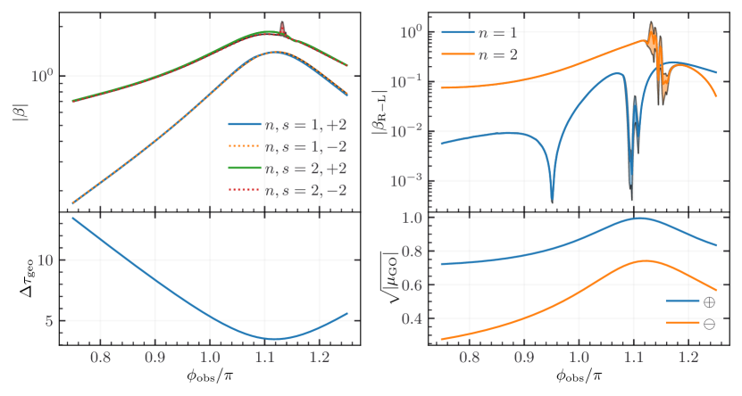
Figure 15: Time delay parametrization upon varying the observer azimuthal angle $\phi_{\rm obs}$. The top row shows $\beta$ and $\beta_{\rm R-L}$. The bottom row shows $\Delta\tau_{\rm geo}$ and $\mu_{\rm GO}$. The source is otherwise at $(2\,R_{\rm s},\pi/2,0)$, observer at $(50\,R_{\rm s},0.4\pi,\phi_{\rm obs})$ and $a=0.99$. We still have that $\alpha\approx 2$ and $\alpha_{\rm R-L}\approx 3$.

We assume the far static observer to follow a worldline $\gamma_{\rm obs}(\tau)$ parameterized in the Boyer-Lindquist coordinate system of a Kerr metric as

$$(\gamma_{\rm obs})^{\mu}(\tau)=\left(t_{\rm obs}(\tau),r_{\rm obs},\theta_{\rm obs},\phi_{\rm obs}\right),$$ (A.1)

where the spatial coordinates $\bm{x}_{\rm obs}=(r_{\rm obs},\theta_{\rm obs},\phi_{\rm obs})$ are constant. Therefore, the $4$-velocity of this observer is

$$\derivative{(\gamma_{\rm obs})^{\mu}}{\tau}=\left(\derivative{t_{\rm obs}(\tau)}{\tau},0,0,0\right),$$ (A.2)

and to ensure that $\gamma_{\rm obs}(\tau)$ is parameterized in terms of observer’s proper time $\tau$ we impose that

$$\tensor{g}{{}_{\mu}{}_{\nu}}\derivative{(\gamma_{\rm obs})^{\mu}}{\tau}\derivative{(\gamma_{\rm obs})^{\mu}}{\tau}=\left.\tensor{g}{{}_{0}{}_{0}}\right|_{\bm{x}_{\rm obs}}\left(\derivative{t_{\rm obs}}{\tau}\right)^{2}=-1.$$ (A.3)

From the above equation, together with the assumption that $\differential\gamma_{\rm obs}/\differential\tau$ is future-directed with respect to the Killing vector field $\partial_{t}$, we obtain

$$\tau=t_{\rm obs}\sqrt{-\left.\tensor{g}{{}_{0}{}_{0}}\right|_{\bm{x}_{\rm obs}}},$$ (A.4)

which, up to a constant addition factor, relates the coordinate time to the observer’s proper time.

A.2 Alignment of an arbitrary tetrad

We consider another orthonormal tetrad $\tilde{e}_{a}$ related to $e_{a}$ by spacetime-dependent boosts, with boost velocity $\bm{v}=(v_{1},v_{2},v_{3})$. The boosted orthonormal tetrad $\tilde{e}_{a}$ can be defined as in Ref. [147, Eq. 9]

$$\tilde{e}_{0} =\frac{e_{0}+v_{1}e_{1}+v_{2}e_{2}+v_{3}e_{3}}{\sqrt{1-v^{2}}},$$ (A.5a)

$$\tilde{e}_{1} =\frac{(1-{v_{2}}^{2})e_{1}+v_{1}(v_{2}e_{2}+e_{0})}{\sqrt{1-{v_{2}}^{2}}\sqrt{1-{v_{1}}^{2}-{v_{2}}^{2}}},$$ (A.5b)

$$\tilde{e}_{2} =\frac{e_{2}+v_{2}e_{0}}{\sqrt{1-{v_{2}}^{2}}},$$ (A.5c)

$$\tilde{e}_{3} =\frac{(1-{v_{1}}^{2}-{v_{2}}^{2})e_{3}+v_{3}(v_{1}e_{1}+v_{2}e_{2}+e_{0})}{\sqrt{1-{v_{1}}^{2}-{v_{2}}^{2}}\sqrt{1-v^{2}}},$$ (A.5d)

where $v^{2}={v_{1}}^{2}+{v_{2}}^{2}+{v_{3}}^{2}<1$. In our case, we consider the original orthonormal tetrad $e_{a}$ to be that of the Kerr metric defined in Equation 2.3.

As discussed in Section A.1, a static observer follows a worldline $\gamma_{\rm obs}(\tau)$. We wish to align $e_{0}$ with $\tilde{e}_{0}$ so that

$$(\tilde{e}_{0})^{\mu}=\derivative{(\gamma_{\rm obs})^{\mu}}{\tau}=1/\sqrt{-\left.\tensor{g}{{}_{0}{}_{0}}\right|_{\bm{x}_{\rm obs}}}\tensor{\delta}{{}^{\mu}_{0}}.$$ (A.6)

Therefore, we will need a boost with $\mathbf{v}=(0,0,v_{3})$, where

$$v_{3}=-\frac{a\sin{\theta_{\rm obs}}}{\sqrt{\Delta(r_{\rm obs})}}e^{-(r-r_{\rm obs})^{2}},$$ (A.7)

where the exponential ensures a smooth alignment from $e_{a}$ far from the observer to $\tilde{e}_{a}$ at the observer’s position. A similar boost can be performed at the source’s location, which will be valid as long as the two exponentials have insignificant overlap.

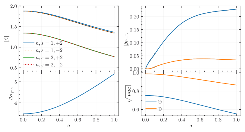
Figure 16: Time delay parametrization upon varying the BH spin $a$. The top row shows $\beta$ and $\beta_{\rm R-L}$. The bottom row shows $\Delta\tau_{\rm geo}$ and $\mu_{\rm GO}$. The source is at $(2\,R_{\rm s},\pi/2,0)$ and the observer at $(50\,R_{\rm s},0.4\pi,\pi)$. We again have that $\alpha\approx 2$ and $\alpha_{\rm R-L}\approx 3$. In the Schwarzschild metric the GSHE-to-geodesic delay is maximized, while the right-to-left delay is zero.

Appendix B Additional time delay scaling

We now continue with the discussion from Section III.1 of the GSHE-induced time delay with respect to the geodesic arrival as a function of the azimuthal separation and the Kerr BH spin.

B.1 Dependence on the azimuthal separation

In Fig. 15, we vary the azimuthal angle of the observer $\phi_{\rm obs}$. The source is at $(2\,R_{\rm s},\pi/2,0)$, the observer is at $(50\,R_{\rm s},0.4\pi,\phi_{\rm obs})$ and $a=0.99$. Because of the nonzero BH spin, the setup is not symmetric around $\phi_{\rm obs}=\pi$ and instead we find that trajectories moving against the direction of the BH spin receive stronger GSHE corrections. There exist symmetric source-observer configurations in which the right-to-left delay appears to vanish, although at present we do not investigate their origin further. When $\phi_{\rm obs}\approx=1.1\pi$ the GSHE corrections and geodesic magnification are maximized. Changing the sign of the BH spin, this point moves as expected to $0.9\pi$.

B.2 Dependence on the BH spin

In Fig. 16, we plot how the time delay parameters of directly connecting bundles – $\beta$, $\beta_{\rm R-L}$, $\Delta\tau_{\rm geo}$ and $\mu_{\rm GO}$ – depend on the BH spin $a$ while keeping the source and observer fixed. The source is placed at $(2\,R_{\rm s},\pi/2,0)$ and the observer at $(50\,R_{\rm s},0.4\pi,\pi)$. We again note that in all cases $\alpha\approx 2$ and $\alpha_{\rm R-L}\approx 3$. The GSHE-to-geodesic delay is maximized when the Kerr metric approaches the Schwarzschild limit, while the right-to-left delay vanishes in the Schwarzschild metric. We attribute the Schwarzschild maximum of the GSHE-to-geodesic delay to the fact that the Kerr BH horizon grows with decreasing spin, and, therefore, the trajectories pass closer to it. There is no GSHE birefringence if the black hole is not spinning because of the reflection symmetry of the Schwarzschild metric. Lastly, we verify that this behavior is not a consequence of a particular source-observer configuration and qualitatively holds in general.

Appendix C Relation between the image parity and the GSHE-to-geodesic delay sign

We investigate the relationship between signal parity and the sign of the GSHE-to-geodesic delay $\Delta\tau(\epsilon,s)$ in the settings of Fig. 7, where we previously calculated $\beta$ as a function of the direction of emission (cf. Section III.1.3). We show this in Fig. 19 for a right-polarized wave ($s=2$), where the red and violet regions correspond to $+1$ and $-1$, respectively. First, in the left panel, the negative time delay corresponds to a well-defined region whose outside boundary is the Kerr equivalent of the Einstein ring, where the determinant of the trajectory mapping approaches zero, or, equivalently, the magnification tends to infinity. This boundary also delineates the middle panel which shows the geodesic parity. However, unlike in the left panel, the negative geodesic parity region extends almost to the BH shadow boundary, where the parity starts to oscillate as the solutions begin to completely loop around the BH. Thus, outside of this, it is only within the central red region of the left panel where the GSHE-to-geodesic delay and image parity signs disagree. For completeness, we also include the magnification at a finite value of $\epsilon$ in the right panel, although it is nearly indistinguishable from the geodesic magnification. Due to the weak dependence on $\epsilon$, we do not expect this picture to change qualitatively for the left polarization. Our results are in agreement with the theory of standard lensing in the weak limit, where trajectories outside the Einstein ring have positive parity and negative parity inside it [89, 91].

Appendix D Dependence on sign of $\beta$ and $N_{\rm loop}$

In this section, we explore some additional details of the GSHE detection likelihood. Fig. 19 shows the dependence of the source’s probabilities on the sign of the time delay. Negative GSHE time delays ($\beta<0$) are less likely when the effect is small, but larger when $\beta_{\min}\gtrsim 1$. As the sign of $\beta$ can be distinguished by observation, this information can be included when computing probabilities.

Fig. 19 depicts the effect of limiting the number of loops on the observer’s probability, without any limit on $|\mu|$. This plot differs from Fig. 10 where no cut on the magnification is employed: trajectories with multiple loops are strongly demagnified ($|\mu|\ll 10^{-3}$), and therefore “spread” widely over all possible observers, leading to $\Upsilon_{\rm obs}\sim\mathcal{O}(10)$, even for $|\beta|\gtrsim 1$. Notably, each number of loops contains two families of trajectories (positive and negative parity). As $\beta_{\min}\to 0$, the $N_{\rm loop}=0$ case approaches the expected value $3/2$, which corresponds to two families of trajectories, with one of them (with weaker deflection) covering only half of the sphere. However, a similar calculation in the multi-loop case is limited by the spatial resolution of our simulations.

Figure 17: Comparison of the GSHE-to-geodesic delay sign (left panel), the geodesic parity (middle panel) and the GSHE parity (right panel). Red and violet denote $+1$ and $-1$, respectively. This is plotted as a function of the initial momenta for a source at $(5\,R_{\rm s},\pi/2,0)$ and $a=0.99$, corresponding to Fig. 7. The GSHE-to-geodesic delay sign is in agreement with the image parity everywhere except in the central red region of the left panel. The GSHE parity approximately agrees with the geodesic parity.

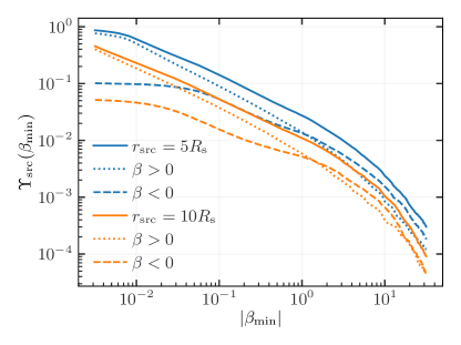
Figure 18: Effect of the sign of $\beta$ on the source’s probability at different source radii.

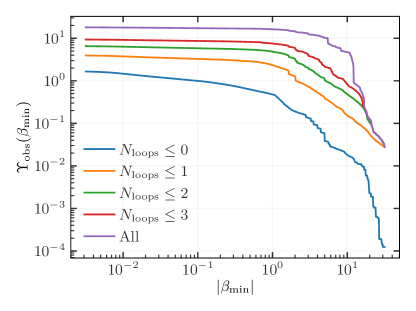
Figure 19: Effect of the number of loops on the observer’s GSHE probability, for any value of $|\mu|$.

References

- The LIGO Scientific Collaboration [2015] The LIGO Scientific Collaboration, Advanced LIGO, Classical and Quantum Gravity 32, 074001 (2015).
- The LIGO Scientific Collaboration and the Virgo Collaboration [2016] The LIGO Scientific Collaboration and the Virgo Collaboration, Observation of Gravitational Waves from a Binary Black Hole Merger, Physical Review Letters 116, 061102 (2016).
- Flanagan and Hughes [2005] É. É. Flanagan and S. A. Hughes, The basics of gravitational wave theory, New Journal of Physics 7, 204 (2005).
- Takahashi and Nakamura [2003] R. Takahashi and T. Nakamura, Wave effects in gravitational lensing of gravitational waves from chirping binaries, The Astrophysical Journal 595, 1039 (2003).
- Çalışkan et al. [2023a] M. Çalışkan, L. Ji, R. Cotesta, E. Berti, M. Kamionkowski, and S. Marsat, Observability of lensing of gravitational waves from massive black hole binaries with lisa, Physical Review D 107, 043029 (2023a).
- Tambalo et al. [2022] G. Tambalo, M. Zumalacárregui, L. Dai, and M. H.-Y. Cheung, Lensing of gravitational waves: efficient wave-optics methods and validation with symmetric lenses, arXiv:2210.05658 (2022).
- Bliokh et al. [2015] K. Y. Bliokh, F. J. Rodríguez-Fortuño, F. Nori, and A. V. Zayats, Spin-orbit interactions of light, Nature Photonics 9, 796 (2015).
- Campanelli et al. [2006] M. Campanelli, C. O. Lousto, and Y. Zlochower, Spin-orbit interactions in black-hole binaries, Physical Review D 74, 084023 (2006).
- Dooghin et al. [1992] A. V. Dooghin, N. D. Kundikova, V. S. Liberman, and B. Y. Zel’dovich, Optical Magnus effect, Physical Review A 45, 8204 (1992).
- Liberman and Zel’dovich [1992] V. S. Liberman and B. Y. Zel’dovich, Spin-orbit interaction of a photon in an inhomogeneous medium, Physical Review A 46, 5199 (1992).
- Onoda et al. [2004] M. Onoda, S. Murakami, and N. Nagaosa, Hall effect of light, Physical Review Letters 93, 083901 (2004).
- Bliokh and Bliokh [2004a] K. Y. Bliokh and Y. P. Bliokh, Modified geometrical optics of a smoothly inhomogeneous isotropic medium: The anisotropy, Berry phase, and the optical Magnus effect, Physical Review E 70, 026605 (2004a).
- Bliokh and Bliokh [2004b] K. Y. Bliokh and Y. P. Bliokh, Topological spin transport of photons: The optical Magnus effect and Berry phase, Physics Letters A 333, 181 (2004b).
- Duval et al. [2006] C. Duval, Z. Horváth, and P. A. Horváthy, Fermat principle for spinning light, Physical Review D 74, 021701 (2006).
- Hosten and Kwiat [2008] O. Hosten and P. Kwiat, Observation of the spin Hall effect of light via weak measurements, Science 319, 787 (2008).
- Aiello and Woerdman [2008] A. Aiello and J. P. Woerdman, Role of beam propagation in Goos–Hänchen and Imbert–Fedorov shifts, Optics Letters 33, 1437 (2008).
- Bliokh et al. [2008] K. Y. Bliokh, A. Niv, V. Kleiner, and E. Hasman, Geometrodynamics of spinning light, Nature Photonics 2, 748 (2008).
- Bliokh [2009] K. Y. Bliokh, Geometrodynamics of polarized light: Berry phase and spin Hall effect in a gradient-index medium, Journal of Optics A: Pure and Applied Optics 11, 094009 (2009).
- Ling et al. [2017] X. Ling, X. Zhou, K. Huang, Y. Liu, C.-W. Qiu, H. Luo, and S. Wen, Recent advances in the spin Hall effect of light, Reports on Progress in Physics 80, 066401 (2017).
- Gosselin et al. [2007a] P. Gosselin, A. Bérard, and H. Mohrbach, Spin Hall effect of photons in a static gravitational field, Physical Review D 75, 084035 (2007a).
- Yamamoto [2018] N. Yamamoto, Spin Hall effect of gravitational waves, Physical Review D 98, 061701 (2018).
- Oancea et al. [2020] M. A. Oancea, J. Joudioux, I. Y. Dodin, D. E. Ruiz, C. F. Paganini, and L. Andersson, Gravitational spin Hall effect of light, Physical Review D 102, 024075 (2020).
- Frolov [2020] V. P. Frolov, Maxwell equations in a curved spacetime: Spin optics approximation, Physical Review D 102, 084013 (2020).
- Andersson et al. [2021] L. Andersson, J. Joudioux, M. A. Oancea, and A. Raj, Propagation of polarized gravitational waves, Physical Review D 103, 044053 (2021).
- Oancea [2021] M. A. Oancea, Spin Hall effects in General Relativity, PhD thesis, University of Potsdam (2021).
- Harte and Oancea [2022] A. I. Harte and M. A. Oancea, Spin Hall effects and the localization of massless spinning particles, Physical Review D 105, 104061 (2022).
- Oancea and Kumar [2023] M. A. Oancea and A. Kumar, Semiclassical analysis of Dirac fields on curved spacetime, Physical Review D 107, 044029 (2023).
- Frolov and Shoom [2011] V. P. Frolov and A. A. Shoom, Spinoptics in a stationary spacetime, Physical Review D 84, 044026 (2011).
- Frolov and Shoom [2012] V. P. Frolov and A. A. Shoom, Scattering of circularly polarized light by a rotating black hole, Physical Review D 86, 024010 (2012).
- Yoo [2012] C.-M. Yoo, Notes on spinoptics in a stationary spacetime, Physical Review D 86, 084005 (2012).
- Harte [2019] A. I. Harte, Gravitational lensing beyond geometric optics: I. Formalism and observables, General Relativity and Gravitation 51, 14 (2019).
- Dolan [2018a] S. R. Dolan, Higher-order geometrical optics for circularly-polarized electromagnetic waves, arXiv:1801.02273 (2018a).
- Dolan [2018b] S. R. Dolan, Geometrical optics for scalar, electromagnetic and gravitational waves on curved spacetime, International Journal of Modern Physics D 27, 1843010 (2018b).
- Shoom [2021] A. A. Shoom, Gravitational Faraday and spin-Hall effects of light, Physical Review D 104, 084007 (2021).
- Audretsch [1981] J. Audretsch, Trajectories and spin motion of massive spin- particles in gravitational fields, Journal of Physics A: Mathematical and General 14, 411 (1981).
- Rüdiger [1981] R. Rüdiger, The Dirac equation and spinning particles in general relativity, Proceedings of the Royal Society A: Mathematical, Physical and Engineering Sciences 377, 417 (1981).
- Gosselin et al. [2007b] P. Gosselin, A. Bérard, and H. Mohrbach, Semiclassical dynamics of Dirac particles interacting with a static gravitational field, Physics Letters A 368, 356 (2007b).
- Souriau [1974] J.-M. Souriau, Modèle de particule à spin dans le champ électromagnétique et gravitationnel, Annales de l’Institut Henri Poincaré A 20, 315 (1974).
- Saturnini [1976] P. Saturnini, Un modèle de particule à spin de masse nulle dans le champ de gravitation, PhD thesis, Université de Provence (1976).
- Duval and Schücker [2017] C. Duval and T. Schücker, Gravitational birefringence of light in Robertson-Walker cosmologies, Physical Review D 96, 043517 (2017).
- Duval et al. [2018] C. Duval, J. Pasquet, T. Schücker, and A. Tilquin, Gravitational birefringence and an exotic formula for redshifts, Physical Review D 97, 123508 (2018).
- Duval et al. [2019] C. Duval, L. Marsot, and T. Schücker, Gravitational birefringence of light in Schwarzschild spacetime, Physical Review D 99, 124037 (2019).
- Andersson and Oancea [2023] L. Andersson and M. A. Oancea, Spin Hall effects in the sky, arXiv:2302.13634 (2023).
- Oancea et al. [2019] M. A. Oancea, C. F. Paganini, J. Joudioux, and L. Andersson, An overview of the gravitational spin Hall effect, arXiv:1904.09963 (2019).
- Abbott et al. [2018a] B. P. Abbott et al. (KAGRA, LIGO Scientific, Virgo, VIRGO), Prospects for observing and localizing gravitational-wave transients with Advanced LIGO, Advanced Virgo and KAGRA, Living Reviews in Relativity 21, 3 (2018a).
- Lu et al. [2014] R.-S. Lu, A. E. Broderick, F. Baron, J. D. Monnier, V. L. Fish, S. S. Doeleman, and V. Pankratius, Imaging the supermassive black hole shadow and jet base of M87 with the Event Horizon Telescope, The Astrophysical Journal 788, 120 (2014).
- Gerosa and Berti [2017] D. Gerosa and E. Berti, Are merging black holes born from stellar collapse or previous mergers?, Physical Review D 95, 124046 (2017).
- Rodriguez et al. [2019] C. L. Rodriguez, M. Zevin, P. Amaro-Seoane, S. Chatterjee, K. Kremer, F. A. Rasio, and C. S. Ye, Black holes: The next generation—repeated mergers in dense star clusters and their gravitational-wave properties, Physical Review D 100, 043027 (2019).
- Fragione et al. [2020] G. Fragione, A. Loeb, and F. A. Rasio, On the Origin of GW190521-like events from repeated black hole mergers in star clusters, The Astrophysical Journal Letters 902, L26 (2020).
- Levin [2007] Y. Levin, Starbursts near supermassive black holes: young stars in the Galactic Center, and gravitational waves in LISA band, Monthly Notices of the Royal Astronomical Society 374, 515 (2007).
- McKernan et al. [2020] B. McKernan, K. E. S. Ford, R. O’Shaughnessy, and D. Wysocki, Monte Carlo simulations of black hole mergers in AGN discs: Low mergers and predictions for LIGO, Monthly Notices of the Royal Astronomical Society 494, 1203 (2020).
- Tagawa et al. [2020] H. Tagawa, Z. Haiman, and B. Kocsis, Formation and Evolution of Compact Object Binaries in AGN Disks, The Astrophysical Journal 898, 25 (2020).
- Gerosa and Fishbach [2021] D. Gerosa and M. Fishbach, Hierarchical mergers of stellar-mass black holes and their gravitational-wave signatures, Nature Astronomy 5, 749 (2021).
- Miralda-Escude and Gould [2000] J. Miralda-Escude and A. Gould, A cluster of black holes at the galactic center, The Astrophysical Journal 545, 847 (2000).
- Bellovary et al. [2016] J. M. Bellovary, M.-M. Mac Low, B. McKernan, and K. E. S. Ford, Migration Traps in Disks Around Supermassive Black Holes, The Astrophysical Journal Letters 819, L17 (2016).
- Peng and Chen [2021] P. Peng and X. Chen, The last migration trap of compact objects in AGN accretion disc, Monthly Notices of the Royal Astronomical Society 505, 1324 (2021).
- Kocsis [2013] B. Kocsis, High Frequency Gravitational Waves from Supermassive Black Holes: Prospects for LIGO-Virgo Detections, Astrophys. J. 763, 122 (2013), arXiv:1211.6427 [astro-ph.HE] .
- D’Orazio and Loeb [2020] D. J. D’Orazio and A. Loeb, Repeated gravitational lensing of gravitational waves in hierarchical black hole triples, Physical Review D 101, 083031 (2020).
- Gondán and Kocsis [2022] L. Gondán and B. Kocsis, Astrophysical gravitational-wave echoes from galactic nuclei, Monthly Notices of the Royal Astronomical Society 515, 3299 (2022).
- Abbott et al. [2020a] R. Abbott et al. (LIGO Scientific, Virgo), GW190521: A Binary Black Hole Merger with a Total Mass of , Physical Review Letters 125, 101102 (2020a).
- Abbott et al. [2020b] R. Abbott et al. (LIGO Scientific, Virgo), Properties and Astrophysical Implications of the 150 M⊙ Binary Black Hole Merger GW190521, The Astrophysical Journal Letters 900, L13 (2020b).
- Farmer et al. [2019] R. Farmer, M. Renzo, S. E. de Mink, P. Marchant, and S. Justham, Mind the Gap: The Location of the Lower Edge of the Pair-instability Supernova Black Hole Mass Gap, The Astrophysical Journal 887, 53 (2019).
- Graham et al. [2020] M. J. Graham et al., Candidate Electromagnetic Counterpart to the Binary Black Hole Merger Gravitational Wave Event S190521g, Physical Review Letters 124, 251102 (2020).
- Nitz and Capano [2021] A. H. Nitz and C. D. Capano, GW190521 may be an intermediate mass ratio inspiral, The Astrophysical Journal Letters 907, L9 (2021).
- Fishbach and Holz [2020] M. Fishbach and D. E. Holz, Minding the gap: GW190521 as a straddling binary, The Astrophysical Journal Letters 904, L26 (2020).
- Calderón Bustillo et al. [2021] J. Calderón Bustillo, S. H. W. Leong, K. Chandra, B. McKernan, and K. E. S. Ford, GW190521 as a black-hole merger coincident with the ZTF19abanrhr flare, arXiv:2112.12481 (2021).
- Estellés et al. [2022] H. Estellés et al., A Detailed Analysis of GW190521 with Phenomenological Waveform Models, The Astrophysical Journal 924, 79 (2022).
- Olsen et al. [2021] S. Olsen, J. Roulet, H. S. Chia, L. Dai, T. Venumadhav, B. Zackay, and M. Zaldarriaga, Mapping the likelihood of GW190521 with diverse mass and spin priors, Physical Review D 104, 083036 (2021).
- Ashton et al. [2021] G. Ashton, K. Ackley, I. M. Hernandez, and B. Piotrzkowski, Current observations are insufficient to confidently associate the binary black hole merger GW190521 with AGN J124942.3 + 344929, Classical and Quantum Gravity 38, 235004 (2021).
- Palmese et al. [2021] A. Palmese, M. Fishbach, C. J. Burke, J. T. Annis, and X. Liu, Do LIGO/Virgo Black Hole Mergers Produce AGN Flares? The Case of GW190521 and Prospects for Reaching a Confident Association, The Astrophysical Journal Letters 914, L34 (2021).
- Amaro-Seoane et al. [2017] P. Amaro-Seoane et al., Laser Interferometer Space Antenna, arXiv:1702.00786 (2017).
- Baker et al. [2019] J. Baker et al., The Laser Interferometer Space Antenna: Unveiling the Millihertz Gravitational Wave Sky, arXiv:1907.06482 (2019).
- Inayoshi et al. [2017] K. Inayoshi, N. Tamanini, C. Caprini, and Z. Haiman, Probing stellar binary black hole formation in galactic nuclei via the imprint of their center of mass acceleration on their gravitational wave signal, Physical Review D 96, 063014 (2017).
- Toubiana et al. [2021] A. Toubiana et al., Detectable environmental effects in GW190521-like black-hole binaries with LISA, Physical Review Letters 126, 101105 (2021).
- Yu and Chen [2021] H. Yu and Y. Chen, Direct determination of supermassive black hole properties with gravitational-wave radiation from surrounding stellar-mass black hole binaries, Physical Review Letters 126, 021101 (2021).
- Sberna et al. [2022] L. Sberna, S. Babak, S. Marsat, A. Caputo, G. Cusin, A. Toubiana, E. Barausse, C. Caprini, T. Dal Canton, A. Sesana, and N. Tamanini, Observing GW190521-like binary black holes and their environment with LISA, Physical Review D 106, 064056 (2022).
- Sedda et al. [2020a] M. A. Sedda, M. Mapelli, M. Spera, M. Benacquista, and N. Giacobbo, Fingerprints of binary black hole formation channels encoded in the mass and spin of merger remnants, The Astrophysical Journal 894, 133 (2020a).
- Zevin et al. [2021] M. Zevin, I. M. Romero-Shaw, K. Kremer, E. Thrane, and P. D. Lasky, Implications of Eccentric Observations on Binary Black Hole Formation Channels, The Astrophysical Journal 921, L43 (2021).
- Vajpeyi et al. [2022] A. Vajpeyi, E. Thrane, R. Smith, B. McKernan, and K. E. S. Ford, Measuring the Properties of Active Galactic Nuclei Disks with Gravitational Waves, The Astrophysical Journal 931, 82 (2022).
- Bartos et al. [2017] I. Bartos, Z. Haiman, Z. Marka, B. D. Metzger, N. C. Stone, and S. Marka, Gravitational-wave localization alone can probe origin of stellar-mass black hole mergers, Nature Communications 8, 831 (2017).
- de Rham et al. [2017] C. de Rham, J. T. Deskins, A. J. Tolley, and S.-Y. Zhou, Graviton Mass Bounds, Reviews of Modern Physics 89, 025004 (2017).
- Ezquiaga and Zumalacárregui [2020] J. M. Ezquiaga and M. Zumalacárregui, Gravitational wave lensing beyond general relativity: Birefringence, echoes, and shadows, Physical Review D 102, 124048 (2020).
- Wang et al. [2022] Y.-F. Wang, S. M. Brown, L. Shao, and W. Zhao, Tests of gravitational-wave birefringence with the open gravitational-wave catalog, Physical Review D 106, 084005 (2022).
- Oancea et al. [2023] M. A. Oancea, R. Stiskalek, and M. Zumalacárregui, Probing general relativistic spin-orbit coupling with gravitational waves from hierarchical triple systems, arXiv:2307.01903 (2023).
- Griffiths and Podolsk\a’y [2009] J. B. Griffiths and J. Podolsk\a’y, Exact space-times in Einstein’s general relativity (Cambridge University Press, 2009).
- Misner et al. [1973] C. W. Misner, K. S. Thorne, and J. A. Wheeler, Gravitation (W. H. Freeman San Francisco, 1973).
- Bliokh and Nori [2012] K. Y. Bliokh and F. Nori, Relativistic Hall Effect, Physical Review Letters 108, 120403 (2012).
- Stone et al. [2015] M. Stone, V. Dwivedi, and T. Zhou, Wigner Translations and the Observer Dependence of the Position of Massless Spinning Particles, Physical Review Letters 114, 210402 (2015).
- Schneider et al. [1992] P. Schneider, J. Ehlers, and E. E. Falco, Gravitational Lenses (Springer-Verlag, Berlin, Heidelberg, New York, 1992).
- Petters et al. [2012] A. O. Petters, H. Levine, and J. Wambsganss, Singularity Theory and Gravitational Lensing, Vol. 21 (Springer Science & Business Media, 2012).
- Dodelson [2017] S. Dodelson, Gravitational Lensing (Cambridge University Press, 2017).
- Sinnott [1984] R. W. Sinnott, Virtues of the Haversine, Sky and Telescope 68, 158 (1984).
- Wolfram Research, Inc. [2021] Wolfram Research, Inc., Mathematica, Version 13.0.0 (2021), Champaign, IL.
- Bezanson et al. [2017] J. Bezanson, A. Edelman, S. Karpinski, and V. B. Shah, Julia: A fresh approach to numerical computing, SIAM Review 59, 65 (2017).
- Rackauckas and Nie [2017] C. Rackauckas and Q. Nie, DifferentialEquations.jl – A Performant and Feature-Rich Ecosystem for Solving Differential Equations in Julia, Journal of Open Research Software 5(1), 15 (2017).
- Mogensen and Riseth [2018] P. K. Mogensen and A. N. Riseth, Optim: A mathematical optimization package for Julia, Journal of Open Source Software 3, 615 (2018).
- Revels et al. [2016] J. Revels, M. Lubin, and T. Papamarkou, Forward-Mode Automatic Differentiation in Julia, arXiv:1607.07892 (2016).
- Nitz et al. [2022] A. Nitz et al., gwastro/pycbc: v2.0.4 release of PyCBC (2022).
- Maggiore [2007] M. Maggiore, Gravitational Waves: Volume 1: Theory and Experiments (Oxford University Press, 2007).
- Williams et al. [2020] D. Williams, I. S. Heng, J. Gair, J. A. Clark, and B. Khamesra, Precessing numerical relativity waveform surrogate model for binary black holes: A Gaussian process regression approach, Physical Review D 101, 063011 (2020).
- Pratten et al. [2021] G. Pratten, C. García-Quirós, M. Colleoni, A. Ramos-Buades, H. Estellés, M. Mateu-Lucena, R. Jaume, M. Haney, D. Keitel, J. E. Thompson, and S. Husa, Computationally efficient models for the dominant and subdominant harmonic modes of precessing binary black holes, Physical Review D 103, 104056 (2021).
- Leite et al. [2017] L. C. S. Leite, S. R. Dolan, and L. C. B. Crispino, Absorption of electromagnetic and gravitational waves by Kerr black holes, Physics Letters B 774, 130 (2017).
- Teukolsky [1973] S. A. Teukolsky, Perturbations of a Rotating Black Hole. I. Fundamental Equations for Gravitational, Electromagnetic, and Neutrino-Field Perturbations, Astrophysical Journal 185, 635 (1973).
- Motohashi and Noda [2021] H. Motohashi and S. Noda, Exact solution for wave scattering from black holes: Formulation, Progress of Theoretical and Experimental Physics 2021, 083E03 (2021).
- Cardoso et al. [2021] V. Cardoso, F. Duque, and G. Khanna, Gravitational tuning forks and hierarchical triple systems, Physical Review D 103, L081501 (2021).
- Feldbrugge et al. [2023] J. Feldbrugge, U.-L. Pen, and N. Turok, Oscillatory path integrals for radio astronomy, Annals of Physics 451, 169255 (2023).
- Hills [1988] J. G. Hills, Hyper-velocity and tidal stars from binaries disrupted by a massive Galactic black hole, Nature 331, 687 (1988).
- Addison et al. [2019] E. Addison, M. Gracia-Linares, P. Laguna, and S. L. Larson, Busting up binaries: encounters between compact binaries and a supermassive black hole, General Relativity and Gravitation 51, 38 (2019).
- Suzuki et al. [2020] H. Suzuki, Y. Nakamura, and S. Yamada, General relativistic effects on Hill stability of multibody systems: Stability of three-body systems containing a massive black hole, Physical Review D 102, 124063 (2020).
- Abbott et al. [2019] B. P. Abbott et al. (LIGO Scientific, Virgo), Tests of General Relativity with the Binary Black Hole Signals from the LIGO-Virgo Catalog GWTC-1, Physical Review D 100, 104036 (2019).
- Abbott et al. [2021a] R. Abbott et al. (LIGO Scientific, Virgo), Tests of general relativity with binary black holes from the second LIGO-Virgo gravitational-wave transient catalog, Physical Review D 103, 122002 (2021a).
- Abbott et al. [2021b] R. Abbott et al. (LIGO Scientific, VIRGO, KAGRA), Tests of General Relativity with GWTC-3, arXiv:2112.06861 (2021b).
- Will [1998] C. M. Will, Bounding the mass of the graviton using gravitational wave observations of inspiralling compact binaries, Physical Review D 57, 2061 (1998).
- Bettoni et al. [2017] D. Bettoni, J. M. Ezquiaga, K. Hinterbichler, and M. Zumalacárregui, Speed of Gravitational Waves and the Fate of Scalar-Tensor Gravity, Physical Review D 95, 084029 (2017).
- Goyal et al. [2023] S. Goyal, A. Vijaykumar, J. M. Ezquiaga, and M. Zumalacarregui, Probing lens-induced gravitational-wave birefringence as a test of general relativity, arXiv:2301.04826 (2023).
- Kostelecky [2004] V. A. Kostelecky, Gravity, Lorentz violation, and the standard model, Physical Review D 69, 105009 (2004).
- Tasson [2016] J. D. Tasson, The Standard-Model Extension and Gravitational Tests, Symmetry 8, 111 (2016).
- Samsing et al. [2022] J. Samsing, I. Bartos, D. J. D’Orazio, Z. Haiman, B. Kocsis, N. W. C. Leigh, B. Liu, M. E. Pessah, and H. Tagawa, AGN as potential factories for eccentric black hole mergers, Nature 603, 237 (2022).
- Levin [2003] Y. Levin, Formation of massive stars and black holes in self-gravitating AGN discs, and gravitational waves in LISA band, arXiv:astro-ph/0307084 (2003).
- McKernan et al. [2012] B. McKernan, K. E. S. Ford, W. Lyra, and H. B. Perets, Intermediate mass black holes in AGN disks: I. Production & Growth, Monthly Notices of the Royal Astronomical Society 425, 460 (2012).
- Häberle et al. [2021] M. Häberle, M. Libralato, A. Bellini, L. L. Watkins, J.-U. Pott, N. Neumayer, R. P. van der Marel, G. Piotto, and D. Nardiello, Hunting for intermediate-mass black holes in globular clusters: an astrometric study of NGC 6441, Monthly Notices of the Royal Astronomical Society 503, 1490 (2021).
- Ford and McKernan [2022] K. E. S. Ford and B. McKernan, Binary black hole merger rates in AGN discs versus nuclear star clusters: loud beats quiet, Monthly Notices of the Royal Astronomical Society 517, 5827 (2022).
- Vijaykumar et al. [2022a] A. Vijaykumar, S. J. Kapadia, and P. Ajith, Can a binary neutron star merger in the vicinity of a supermassive black hole enable a detection of a post-merger gravitational wave signal?, Monthly Notices of the Royal Astronomical Society 513, 3577 (2022a).
- Abbott et al. [2021c] R. Abbott et al. (LIGO Scientific, VIRGO), Search for Lensing Signatures in the Gravitational-Wave Observations from the First Half of LIGO–Virgo’s Third Observing Run, The Astrophysical Journal 923, 14 (2021c).
- Dai et al. [2020] L. Dai, B. Zackay, T. Venumadhav, J. Roulet, and M. Zaldarriaga, Search for Lensed Gravitational Waves Including Morse Phase Information: An Intriguing Candidate in O2, arXiv:2007.12709 (2020).
- Janquart et al. [2022] J. Janquart, O. A. Hannuksela, K. Haris, and C. Van Den Broeck, GOLUM: A fast and precise methodology to search for, and analyze, strongly lensed gravitational-wave events, arXiv:2203.06444 (2022).
- Çalışkan et al. [2023b] M. Çalışkan, J. M. Ezquiaga, O. A. Hannuksela, and D. E. Holz, Lensing or luck? false alarm probabilities for gravitational lensing of gravitational waves, Physical Review D 107, 063023 (2023b).
- Dai and Venumadhav [2017] L. Dai and T. Venumadhav, On the waveforms of gravitationally lensed gravitational waves, arXiv:1702.04724 (2017).
- Ezquiaga et al. [2021] J. M. Ezquiaga, D. E. Holz, W. Hu, M. Lagos, and R. M. Wald, Phase effects from strong gravitational lensing of gravitational waves, Physical Review D 103, 064047 (2021).
- Vijaykumar et al. [2022b] A. Vijaykumar, A. K. Mehta, and A. Ganguly, Detection and parameter estimation challenges of Type-II lensed binary black hole signals, arXiv:2202.06334 (2022b).
- Lindblom et al. [2008] L. Lindblom, B. J. Owen, and D. A. Brown, Model waveform accuracy standards for gravitational wave data analysis, Physical Review D 78, 124020 (2008).
- Paynter et al. [2021] J. Paynter, R. Webster, and E. Thrane, Evidence for an intermediate-mass black hole from a gravitationally lensed gamma-ray burst, Nature Astronomy 5, 560 (2021).
- Kalantari et al. [2021] Z. Kalantari, A. Ibrahim, M. R. R. Tabar, and S. Rahvar, Imprints of Gravitational Millilensing on the Light Curve of Gamma-Ray Bursts, The Astrophysical Journal 922, 77 (2021).
- Wang et al. [2021] Y. Wang, L.-Y. Jiang, C.-K. Li, J. Ren, S.-P. Tang, Z.-M. Zhou, Y.-F. Liang, and Y.-Z. Fan, GRB 200716C: Evidence for a Short Burst Being Lensed, The Astrophysical Journal Letters 918, L34 (2021).
- Husa et al. [2016] S. Husa, S. Khan, M. Hannam, M. Pürrer, F. Ohme, X. Jiménez Forteza, and A. Bohé, Frequency-domain gravitational waves from nonprecessing black-hole binaries. I. New numerical waveforms and anatomy of the signal, Physical Review D 93, 044006 (2016).
- Chen et al. [2021] H.-Y. Chen, D. E. Holz, J. Miller, M. Evans, S. Vitale, and J. Creighton, Distance measures in gravitational-wave astrophysics and cosmology, Classical Quantum Gravity 38, 055010 (2021).
- Abbott et al. [2018b] B. P. Abbott et al. (KAGRA, LIGO Scientific, Virgo, VIRGO), Prospects for observing and localizing gravitational-wave transients with Advanced LIGO, Advanced Virgo and KAGRA, Living Reviews in Relativity 21, 3 (2018b).
- Reitze et al. [2019] D. Reitze et al., Cosmic Explorer: The U.S. Contribution to Gravitational-Wave Astronomy beyond LIGO, Bulletin of the American Astronomical Society 51, 035 (2019).
- Maggiore et al. [2020] M. Maggiore et al., Science case for the Einstein telescope, Journal of Cosmology and Astroparticle Physics 2020 (3), 050.
- Kalogera et al. [2021] V. Kalogera et al., The Next Generation Global Gravitational Wave Observatory: The Science Book, arXiv:2111.06990 (2021).
- Lindblom et al. [2008] L. Lindblom, B. J. Owen, and D. A. Brown, Model Waveform Accuracy Standards for Gravitational Wave Data Analysis, Physical Review D 78, 124020 (2008).
- Baker et al. [2021] J. Baker et al., High angular resolution gravitational wave astronomy, Experimental Astronomy 51, 1441 (2021).
- Baibhav et al. [2021] V. Baibhav et al., Probing the nature of black holes: Deep in the mHz gravitational-wave sky, Experimental Astronomy 51, 1385 (2021).
- Sedda et al. [2020b] M. A. Sedda et al., The missing link in gravitational-wave astronomy: discoveries waiting in the decihertz range, Classical and Quantum Gravity 37, 215011 (2020b).
- Sesana et al. [2021] A. Sesana et al., Unveiling the gravitational universe at -Hz frequencies, Experimental Astronomy 51, 1333 (2021).
- Gong et al. [2021] Y. Gong, J. Luo, and B. Wang, Concepts and status of Chinese space gravitational wave detection projects, Nature Astronomy 5, 881 (2021).
- Grenzebach et al. [2015] A. Grenzebach, V. Perlick, and C. Lämmerzahl, Photon regions and shadows of accelerated black holes, International Journal of Modern Physics D 24, 1542024 (2015).