Time rescaling of a primal-dual dynamical system with asymptotically vanishing damping
Abstract
In this work, we approach the minimization of a continuously differentiable convex function under linear equality constraints by a second-order dynamical system with an asymptotically vanishing damping term. The system under consideration is a time rescaled version of another system previously found in the literature. We show fast convergence of the primal-dual gap, the feasibility measure, and the objective function value along the generated trajectories. These convergence rates now depend on the rescaling parameter, and thus can be improved by choosing said parameter appropriately. When the objective function has a Lipschitz continuous gradient, we show that the primal-dual trajectory asymptotically converges weakly to a primal-dual optimal solution to the underlying minimization problem. We also exhibit improved rates of convergence of the gradient along the primal trajectories and of the adjoint of the corresponding linear operator along the dual trajectories. Even in the unconstrained case, some trajectory convergence result seems to be new. We illustrate the theoretical outcomes through numerical experiments.
Key Words. Augmented Lagrangian method, primal-dual dynamical system, damped inertial dynamics, Nesterov’s accelerated gradient method, Lyapunov analysis, time rescaling, convergence rate, trajectory convergence
AMS subject classification. 37N40, 46N10, 65K10, 90C25
1 Introduction
1.1 Problem statement and motivation
In this paper we will consider the optimization problem
| (1.1) |
where
| (1.2) |
This model formulation underlies many important applications in various areas, such as image recovery [30], machine learning [25, 36], the energy dispatch of power grids [47, 48], distributed optimization [37, 50] and network optimization [45, 49].
In recent years, there has been a flurry of research on the relationship between continuous time dynamical systems and the numerical algorithms that arise from their discretizations. For the unconstrained optimization problem, it has been known that inertial systems with damped velocities enjoy good convergence properties. For a convex, smooth function , Polyak is the first to consider the heavy ball with friction (HBF) dynamics [43, 42]
| (HBF) |
Alvarez and Attouch continue the line of this study, focusing on inertial dynamics with a fixed viscous damping coefficient [2, 3, 14]. Later on, Cabot, Engler, and Gadat [26, 27] consider the system that replaces with a time dependent damping coefficient . In [46], Su, Boyd, and Candès showed that it turns out one can achieve fast convergence rates by introducing a time dependent damping coefficient which vanishes in a controlled manner, neither too fast nor too slowly, as goes to infinity
| (AVD) |
For , the authors showed that a solution to (AVD) satisfies as . In fact, the choice provides a continuous limit counterpart to Nesterov’s celebrated accelerated gradient algorithm [39, 40, 19]. Weak convergence of the trajectories to minimizers of when has been shown by Attouch, Chbani, Peypouquet, and Redont in [17] and May in [38], together with the improved rates of convergence as . In the meantime, similar results for the discrete counterpart were also reported by Chambolle and Dossal in [28], and by Attouch and Peypouquet in [15] .
In [10], Attouch, Chbani, and Riahi proposed an inertial proximal type algorithm, which results from a discretization of the time rescaled (AVD) system
where is the time scaling function satisfies a certain growth condition and that also enter into convergence rate statement as . The resulting algorithm obtained by the authors is considerably simpler than the founding proximal point algorithm proposed by Güler in [31], while providing comparable convergence rates for the functional values.
In order to approach constrained optimization problems, Augmented Lagrangian Method (ALM) [44] (for linearly constrained problems) and Alternating Direction Method of Multipliers (ADMM) [29, 25] (for problems with separable objectives and block variables linearly coupled in the constraints) and some of their variants have been shown to enjoy substantial success. Continuous-time approaches for structured convex minimization problems formulated in the spirit of the full splitting paradigm have been recently addressed in [24] and, closely connected to our approach, in [49, 32, 6, 23], to which we will have a closer look in Subsection 2.2. The temporal discretization resulting from these dynamics gives rise to the numerical algorithm with fast convergence rates [34, 33] and with a convergence guarantee for the generated iterate [22], without additional assumptions such as strong convexity.
In this paper, we will investigate a second-order dynamical system with asymptotic vanishing damping and time rescaling term, which is associated with the optimization problem (1.1) and formulated in terms of its augmented Lagrangian. The case when the time rescaling term does not appear has been established in [23]. We show that by introducing this time rescaling function, we are able to derive faster convergence rates for the primal-dual gap, the feasibility measure, and the objective function value along generated trajectories while still maintaining the asymptotic behaviour of the trajectories towards a primal-dual optimal solution. On the other hand, this work can also be viewed as an extension of the time rescaling technique derived in [10, 13] for the constrained case. To our knowledge, the trajectory convergence for dynamics with time scaling seems to be new, even in the unconstrained case.
1.2 Notations and a preliminary result
For both Hilbert spaces and , the Euclidean inner product and the associated norm will be denoted by and , respectively. The Cartesian product will be endowed with the inner product and the associated norm defined for as
respectively.
Let be a continuously differentiable convex function such that is Lipschitz continuous. For every it holds (see [40, Theorem 2.1.5])
| (1.3) |
2 The primal-dual dynamical approach
2.1 Augmented Lagrangian formulation
Consider the saddle point problem
| (2.1) |
associated to problem (1.1), where denotes the Lagrangian function
Under the assumptions (1.2), is convex with respect to and affine with respect to . A pair is said to be a saddle point of the Lagrangian function if for every
| (2.2) |
If is a saddle point of then is an optimal solution of (1.1), and is an optimal solution of its Lagrange dual problem. If is an optimal solution of (1.1) and a suitable constraint qualification is fulfilled, then there exists an optimal solution of the Lagrange dual problem such that is a saddle point of . For details and insights into the topic of constraint qualifications for convex duality we refer to [18, 20].
The set of saddle points of , called also primal-dual optimal solutions of (1.1), will be denoted by and, as stated in the assumptions, it will be assumed to be nonempty. The set of feasible points of (1.1) will be denoted by and the optimal objective value of (1.1) by .
The system of primal-dual optimality conditions for (1.1) reads
| (2.3) |
where denotes the adjoint operator of .
2.2 The primal-dual asymptotic vanishing damping dynamical system with time rescaling
The dynamical system which we associate to (1.1) and investigate in this paper reads (2.6) where , , , is a nonnegative continuously differentiable function and are the initial conditions. Replacing the expressions of the partial gradients of into the system leads to the following formulation for (2.6):
The case (2.6) in which there is no time rescaling, i.e., when , was studied by Zeng, Lei, and Chen in [49], and by Boţ and Nguyen in [23]. The system with more general damping, extrapolation and time rescaling coefficients was addressed by He, Hu, and Fang in [32, 35] and by Attouch, Chbani, Fadili, and Riahi in [6].
It is well known that the viscous damping term has a vital role in achieving fast convergence in unconstrained minimization [7, 9, 38]. The role of the extrapolation is to induce more flexibility in the dynamical system and in the associated discrete schemes, as it has been recently noticed in [6, 11, 32, 49]. The time scaling function has the role to further improve the rates of convergence of the objective function value along the trajectory, as it was noticed in the context of uncostrained minimization problems in [5, 10, 12] and of linearly constrained minimization problems in [6, 35].
Finally, we mention that extending the results in this paper to the multi-block case is possible. For further details, we refer the readers to [23, Section 2.4].
2.3 Associated monotone inclusion problem
The optimality system (2.3) can be equivalently written as
| (2.7) |
where
is the maximally monotone operator associated with the convex-concave function . Indeed, it is immediate to verify that is monotone. Since it is also continuous, it is maximally monotone (see, for instance, [18, Corollary 20.28]). Therefore can be interpreted as the set of zeros of the maximally monotone operator , which means that it is a closed convex subset of (see, for instance, [18, Proposition 23.39]).
Even in the non-rescaling case, applying the fast continuous-time approaches recently proposed in [16, 4] to the solving of (2.7) would require the use of the Moreau-Yosida approximation of the operator , for which in general no closed formula is available. The resulting dynamical system would therefore not be formulated in the spirit of the full splitting algorithm, which is undesirable from the point of view of numerical computations. We mention the work [21], which is related to this time rescaling approach.
3 Faster convergence rates via time rescaling
In this section we will derive fast convergence rates for the primal-dual gap, the feasibility measure, and the objective function value along the trajectories generated by the dynamical system (2.6).
We will make the following assumptions on the parameters , , and the function throughout this section.
Assumption 1.
In (2.6), assume that is continuously differentiable. Moreover, suppose that the parameters , and the function satisfy
(3.1)
Besides the first three conditions that are known previously in [23], it is worth pointing out that we can deduce from the last one the following inequality for every :
| (3.2) |
This gives a connection to the condition which appears in [10]. A few more comments regarding the function will come later, after the convergence rates statements.
3.1 The energy function
Let be a solution of (2.6). Let be fixed, we define the energy function
| (3.3) |
where
| (3.4) | ||||
| (3.5) |
Notice that due to (3.8), we have
| (3.6) |
In addition, according to (2.4) and (2.5), we have for every
| (3.7) | ||||
| (3.8) |
where denotes the optimal objective value of (1.1).
Assumption 1 implies the nonnegativity of following quantity, which will appear many times in our analysis:
| (3.9) |
Lemma 3.1.
Let be a solution of (2.6) and . For every it holds
Proof.
Let be fixed. Since , we have
Under these expressions, the system (2.6) can be equivalently written as
which leads to
We get from the distributive property of inner product
Since , the last four terms in the above identity vanish. Indeed,
Therefore, differentiating with respect to gives
| (3.10) |
Furthermore, the convexity of and the fact that guarantee
| (3.11) | ||||
where we recall that the second equality comes from (2.5). By multiplying this inequality by and combining it with (3.10), the coefficient attached to the primal-dual gap becomes
which finally gives the desired statement. ∎
Theorem 3.2.
Let be a solution of (2.6) and . The following statements are true:
-
(i)
it holds
(3.12) (3.13) (3.14) -
(ii)
if, in addition, and , then the trajectory is bounded and the convergence rate of its velocity is
Proof.
(i) Recall that Assumption 1 implies for all and . Moreover, yields . Therefore, we can apply observation (3.8) and Lemma 3.1 to obtain, for every ,
| (3.15) | ||||
| (3.16) |
This means that is nonincreasing on . For every , by integrating (3.16) from to , we obtain
where the last inequality follows from (3.6). Since all quantities inside the integrals are nonnegative, we obtain (3.12)-(3.14) by letting .
(ii) Inequality (3.16) tells us that is nonincreasing on . Hence, for every it holds
| (3.17) |
Assuming and , we immediately see . From (3.17) we obtain, for every ,
| (3.18) |
which implies the boundedness of the trajectory. On the other hand, the same inequality gives for all
| (3.19) |
Using the triangle inequality and (3.18), we obtain for all
| (3.20) |
which gives the desired convergence rate. ∎
3.2 Fast convergence rates for the primal-dual gap, the feasibility measure and the objective function value
The following are the main convergence rates results of the paper.
Theorem 3.3.
Let be a solution of (2.6) and . The following statements are true:
-
(i)
for every it holds
(3.21) -
(ii)
for every it holds
(3.22) where
-
(iii)
for every it holds
(3.23)
Proof.
(i) We have already established that is nonincreasing on . Therefore, from the expression for and relation (3.7) we deduce
| (3.24) |
and the first claim follows.
(ii) From the second line of (2.6), for every we have
| (3.25) |
Fix . On the one hand, integration by parts yields
| (3.26) |
On the other hand, again integrating by parts leads to
| (3.27) |
Now, integrating (3.25) from to and using (3.26) and (3.27) gives us
| (3.28) |
It follows that, for every , we have
| (3.29) |
where
and this quantity is finite in light of (3.20) and (3.18). Now, we set
and we apply Lemma A.1 to deduce that
| (3.30) |
Some comments regarding the previous proof and results are in order.
Remark 3.4.
The proof we provided here is significantly shorter than the one derived in [23] thanks to Lemma A.1. This Lemma is inspired by the one used in [34] for showing the fast convergence to zero of the feasibility measure, although the authors study a different dynamical system. On the other hand, when , the results in [23] is more robust than the one we obtain here, as it gives the rates for the sum of primal-dual gap and feasibility measure, rather than each one individually.
Remark 3.6.
To further illustrate, notice that
fulfills Assumption 1 provided that . Therefore, all the statements derived are above are of order . If we desire to obtain fast convergence rates, we must take small, which in the light of Assumption 1 can be achieved by choosing large enough . Such behavior can be seen in the unconstrained case [10] and other settings [35, 21].
4 Weak convergence of the trajectory to a primal-dual solution
In this section we will show that the solutions to (2.6) weakly converge to an element of .
The fact that enters the convergence rate statement suggests that one can benefit from this time rescaling function when it is at least nondecreasing on . We are, in fact, going to need this condition when showing trajectory convergence.
Assumption 2.
In (2.6), assume that is -Lipschitz continuous for some and that is continuously differentiable and nondecreasing. Moreover, suppose that the parameters , and the function satisfy
Assumption 2 entails the existence of such that
| (4.1) |
and therefore it follows further from the nondecreasing property of that
| (4.2) |
Moreover, from (4.1), for every , we have
which gives
| (4.3) |
We also mention that in the setting of Assumption 2, the dynamical system (2.6) has a unique global twice continuously differentiable solution. The proof follows the same argument as in [23, Theorem 4.1], which relies on the fact that (2.6) can be rewritten as a first-order dynamical system. More precisely, is a solution to (2.6) if and only if is a solution to
where is given by
We omit the details proof and only state the result in the following theorem.
Theorem 4.1.
For every choice of initial conditions
the system (2.6) has a unique global twice continuously differentiable solution .
The additional Lipschitz continuity condition of and the fact that is nondecreasing give rise to the following two essential integrability statements.
Proof.
Now, for a given primal-dual solution , we define the following mappings on
| (4.6) | ||||
| (4.7) |
Lemma 4.3.
Let a solution of (2.6) and . The following inequality holds for every :
| (4.8) |
Proof.
Fix . Differentiating with respect to time yields
Recall the formulas for the gradients of :
since . Plugging this into the expression for gives us
By regrouping and using (2.6), we arrive at
| (4.9) |
On the other hand, by the chain rule, we have
By combining these relations, (2.6) and the fact that , we get
| (4.10) |
The Lipschitz continuity of entails
This, together with (4.10), implies
| (4.11) |
Multiplying (4.9) by and then adding the result to (4.11) yields
where the last inequality follows from Assumption 2:
The desired result then follows after some rearranging. ∎
The following lemma ensures that the first condition of Opial’s Lemma is met.
Lemma 4.4.
Let be a solution to (2.6) and . Then the positive part of belongs to and the limit exists.
Proof.
For any , we multiply (4.3) by and drop the last two norm squared terms to obtain
Recall from (4.6) that for every we have
| (4.12) |
On the one hand, according to (3.14), the second summand of the previous expression belongs to . On the other hand, using (4.3) and (3.12), we assert that
Hence, the first summand of (4.12) also belongs to , which implies that the mapping belongs to as well. For achieving the desired conclusion, we make use of Lemma A.4 with and . ∎
The following results guarantee that the second condition of Opial’s Lemma is also met.
Lemma 4.5.
Let be a solution to (2.6) and . The following inequality holds for every
Proof.
Let be fixed. From (2.6) and the fact that , we have
| (4.13) |
Again using (2.6) yields
| (4.14) |
Adding (4.13) and (4.14) together produces
| (4.15) |
On the one hand, we have
| (4.16) |
On the other hand, it holds
| (4.17) |
Moreover,
| (4.18) |
Now, using (4.16), (4.17) and (4.18) in (4.15) yields
Finally, since
the conclusion follows after dividing the inequality by . ∎
The following proposition provides us with the main integrability result that will be used for verifying the second condition of Opial’s Lemma.
Proposition 4.6.
Let be a solution to (2.6) and . Then it holds
| (4.19) |
Proof.
Recall that from Lemma 4.3, for every , we have
Now, to this inequality we add the one produced by Lemma 4.5. For every , it holds
| (4.20) |
where
Mutiplying (4.20) by and integrating from to , we obtain
| (4.21) |
where
We will furnish five different inequalities from computing each of these integrals separately. Let be fixed.
The integral . By the chain rule, for it holds
which leads to
| (4.22) |
The integral . Integration by parts gives
which implies
| (4.23) |
The integral . Again by integrating by parts, we get
For , according to Assumption 2 we have , hence is monotonically increasing and therefore
It follows that
| (4.24) |
The integral . Yet again, integration by parts produces
and from here
| (4.25) |
The integral . Integration by parts entails
By the Cauchy-Schwarz inequality, we deduce that
and thus
| (4.26) |
Now, to the equality (4.25), we add the inequalities (4.22), (4.23), (4.24) and (4.26) and then proceed to employ (4.21):
| (4.27) |
where, for ,
and the constant is given by
Now we divide (4.27) by , thus obtaining
Now, we integrate this inequality from to . We get
| (4.28) |
We now recall some important facts. First of all, we have
| (4.29) |
In addition, according to Lemma A.2, it holds
| (4.30) |
and
| (4.31) |
respectively. Finally, integrating by parts leads to
| (4.32) |
The supremum term is finite due to the boundedness of the trajectory. Now, by using the nonnegativity of and the facts (4.29), (4.30), (4) and (4.32) on (4.28), we come to
| (4.33) |
where
According to (3.13) and (3.14) in Theorem 3.2, as well as Lemma 4.4, we know that the mappings and belong to . Therefore, by taking the limit as in (4.33) we obtain
Again, from (4.3) we conclude that
which completes the proof. ∎
The following result is the final step towards the second condition of Opial’s Lemma.
Theorem 4.7.
Proof.
We first show the gradient rate. For , it holds
| (4.35) |
On the one hand, by Assumption 2, we can write
| (4.36) |
Since is nondecreasing, for we have . Set . Therefore, for it holds
and thus
| (4.37) |
On the other hand, for every we deduce
| (4.38) |
where the last inequality is a consequence of the -Lipschitz continuity of . By combining (4.36), (4.37) and (4.38), from (4.35) we assert that for every
According to (3.14) and (4.4), the right hand side of the previous inequality belongs to . Since is nondecreasing, for every we have
so
| (4.39) |
i.e., the function being differentiated also belongs to . Therefore, Lemma A.3 gives us
Proceeding in the exact same way, for every we have
According to (3.14) and (4.19), the right hand side of the previous inequality belongs to . Arguing as in (4.39), we deduce that the function being differentiated also belongs to . Again applying Lemma A.3, we come to
Finally, recalling that , we deduce from the triangle inequality that
and the third claim follows. ∎
Remark 4.8.
We now come to the final step and show weak convergence of the trajectories of (2.6) to elements of .
Theorem 4.9.
Proof.
For proving this theorem, we make use of Opial’s Lemma (see Lemma A.5). Lemma 4.4 tells us that exists for every , which proves condition (i) of Opial’s Lemma.
In order to show condition (ii), we recall the operator defined in (2.7) by
Fix (in other words, ) and take any weak sequential cluster point of as , which means there exists a strictly increasing sequence such that
Given that is nondecreasing on , from Theorem 4.7 and (3.22) we deduce that
as . Since , the previous three statements imply
Since we already had as , and the graph of is sequentially closed in (see [18, Proposition 20.38(ii)]), we finally come to
which is to say, . The proof is thus concluded. ∎
Remark 4.10.
In case and , the optimization problem (1.1) reduces to the unconstrained optimization problem
| (4.40) |
Indeed, the system of optimality conditions (2.3) read in this case
in particular, is an optimal solution of (4.40) if and only if . The system (2.6) becomes
The dynamical system in is reads
for , and is nothing else than Nesterov’s accelerated gradient system. The trajectory generated by the system in is for every . The parameters and plays no role in the system. Therefore, the condition on now becomes
If , then Theorem 3.3 (iii) says that converges to with a rate of convergence of as , which is the rate derived in [10, 13].
5 Numerical experiments
We will illustate the theoretical results by two numerical examples, with and . We will address two minimization problems with linear constraints; one with a strongly convex objective function and another with a convex objective function which is not strongly convex. In both cases, the linear constraints are dictated by
Example 5.1.
Consider the minimization problem
The optimality conditions can be calculated and lead to the following primal-dual solution pair
Example 5.2.
Consider the minimization problem
This problem is similar to the regularized logistic regression frequently used in machine learning. We cannot explicitly calculate the optimality conditions as in the previous case; instead, we use the last solution in the numerical experiment as the approximate solution.
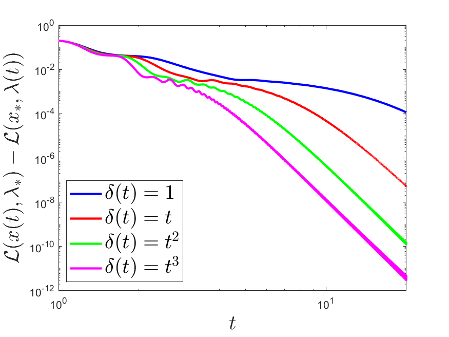
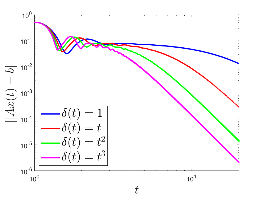
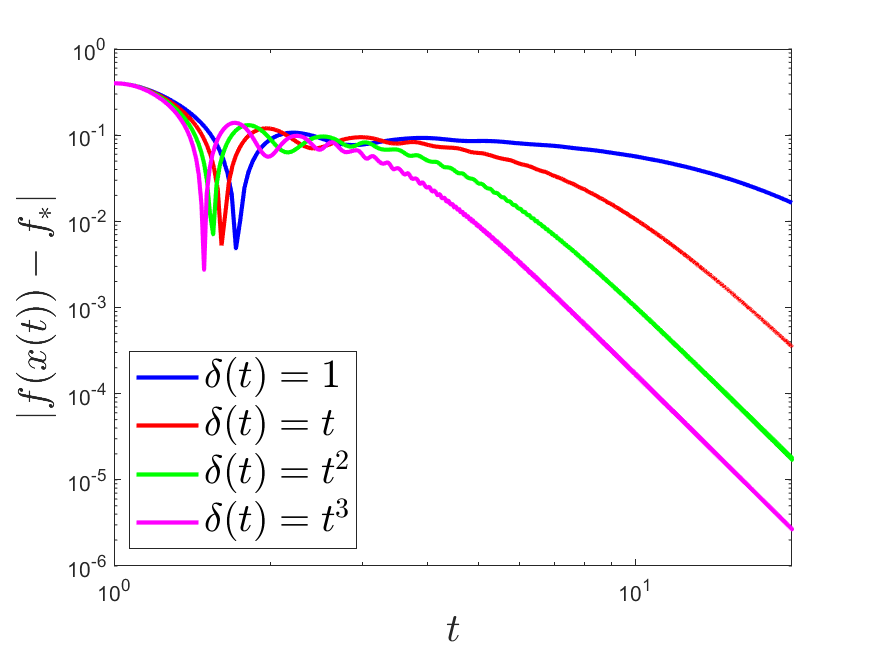
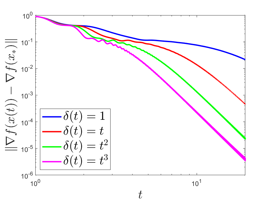
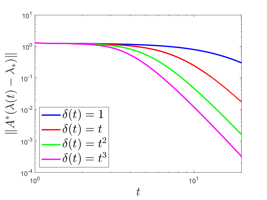
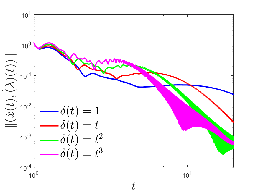
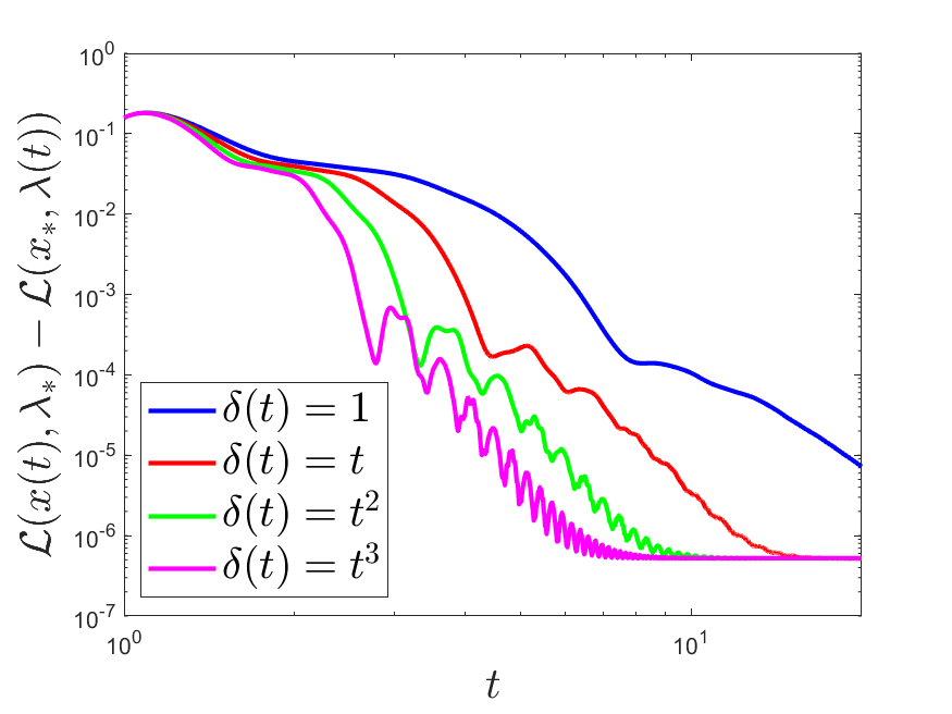
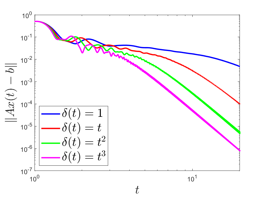
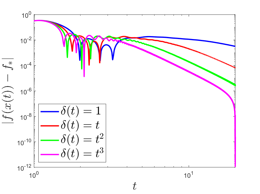
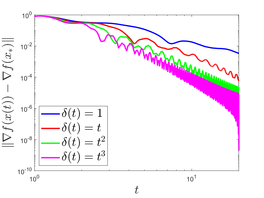
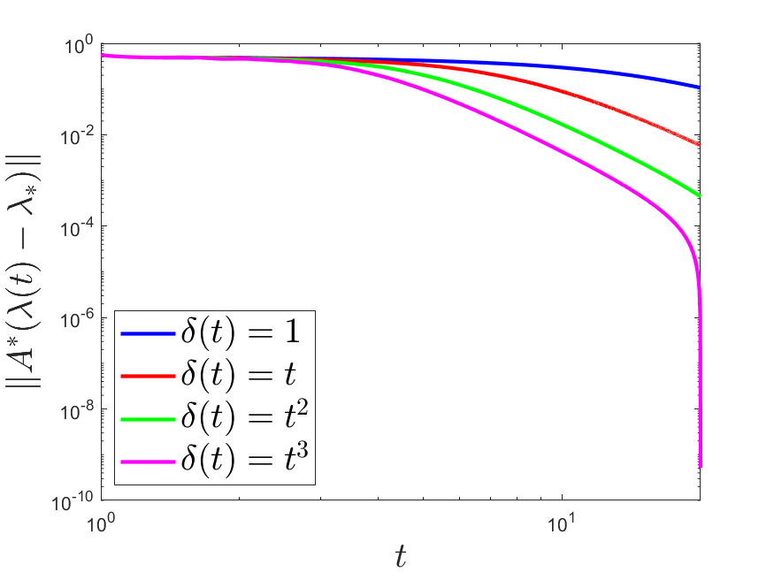
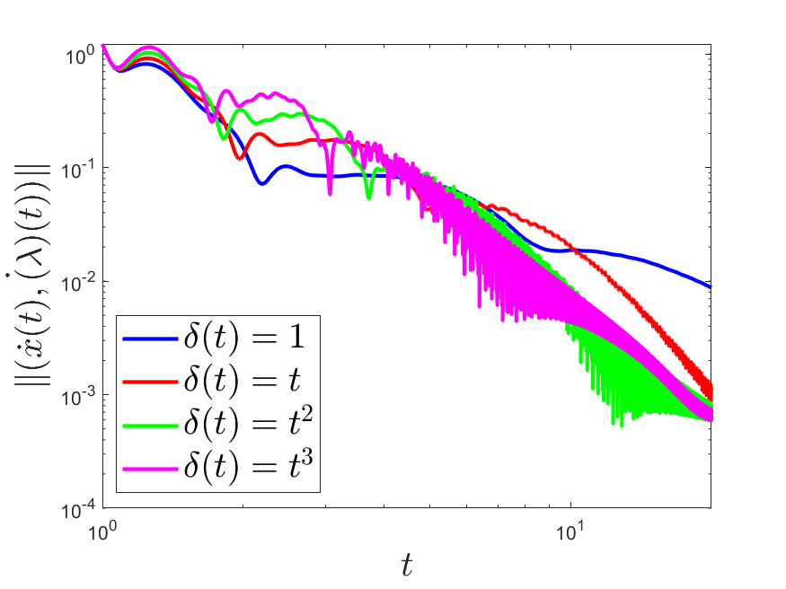
To comply with Assumption 2, we choose , , , , and we test four different choices for the rescaling parameter: (i.e., the (PD-AVD) dynamics in [49, 23]), , and . In both examples, the initial conditions are
For each choice of , we plot, using a logarithmic scale, the primal-dual gap , the feasibility measure and the functional values , to highlight the theoretical result in Theorem 3.3. We also illustrate the findings from Theorem 4.7, namely, we plot the quantities and , as well as the velocity .
Figure 5.1 and 5.2 display these plots for Example 5.1 and 5.2, respectively. As predicted by the theory, choosing faster-growing time rescaling parameters yields better convergence rates. This is not the case for the velocities.
Appendix A Appendix
Here we collect the auxiliary results that are required to carry out many steps in out analysis.
A proof for the following lemma in the finite-dimensional case can be found in [34, Lemma 6]. The proof for the infinite-dimensional case is short and virtually identical, so we include it here for the sake of completeness..
Lemma A.1.
Assume that , is a continuous differentiable function, is a continuous function, and . If, in the sense of Bochner integrability, we have
| (A.1) |
then
Proof.
Define, for every ,
Fix . The time derivative of reads
so by using (A.1) and the previous equality we arrive at
| (A.2) |
Since , we have
so by employing (A.2) and the previous equality we obtain, for every ,
Dividing both sides of the previous inequality by gives us
| (A.3) |
Now, by putting (A.1) and (A.3) we finally come to
which leads to the announced statement. ∎
The proofs for the following results can be found in [23, Lemma A.1] and [1, Lemma 5.2], respectively.
Lemma A.2.
Let and be a continuous function. For every it holds
If , then equality holds.
Lemma A.3.
Let , and . Suppose that is a locally absolutely continuous nonnegative function, and
Then, .
The following lemma is a slight variation of results already present in the literature. See, for example, [8, Lemma A.2].
Lemma A.4.
Let , , and let be a twice continuously differentiable function bounded from below. Furthermore, assume to be a continuously differentiable function such that belongs to and
Then, the positive part of belongs to and the limit is a real number.
Proof.
Fix . Adding to both sides of the previous inequality and then multiplying it by yields
Since the previous inequality holds for any , we can integrate it from to to get
After dropping the nonnegative term and dividing by we arrive at
where
which further leads to
Now, we integrate this inequality from to and we apply Lemma A.2 with given by to obtain
By hypothesis, as , the right hand side of the previous inequality is finite. In other words,
The previous statement, together with the fact that we assumed that was bounded from below, allow us to deduce that the function given by
is also bounded from below. An easy computation shows that is nonpositive on , thus is nonincreasing on . These facts imply that is a real number. Finally, we conclude that
∎
The proof for Opial’s Lemma can be found in [41].
Lemma A.5 (Opial’s Lemma).
Let be a real Hilbert space, a nonempty set, and a mapping that satisfies
-
(i)
for every , exists;
-
(ii)
every weak sequential cluster point of the trajectory as belongs to .
Then, converges weakly to an element of as .
References
- [1] B. Abbas, H. Attouch, B.F. Svaiter. Newton-like dynamics and forward–backward methods for structured monotone inclusions in Hilbert spaces. Journal of Optimization Theory and Applications 161(2), 331–360 (2014)
- [2] F. Alvarez. On the minimizing property of a second order dissipative system in Hilbert spaces. SIAM Journal on Control and Optimization 38(4), 1102–1119 (2000)
- [3] F. Alvarez, H. Attouch, J. Bolte, P. Redont. A second-order gradient-like dissipative dynamical system with Hessian-driven damping: Application to optimization and mechanics. Journal de Mathématiques Pures et Appliquées 81(8), 747–779 (2002)
- [4] H. Attouch. Fast inertial proximal ADMM algorithms for convex structured optimization with linear constraint. Minimax Theory and its Applications 6(1), 1–24 (2021)
- [5] H. Attouch, Z. Chbani, J. Fadili, H. Riahi. First-order optimization algorithms via inertial systems with Hessian driven damping. Mathematical Programming 193, 113–155 (2022)
- [6] H. Attouch, Z. Chbani, J. Fadili, H. Riahi. Fast convergence of dynamical ADMM via time scaling of damped inertial dynamics. Journal of Optimization Theory and Applications 193, 704–736 (2022)
- [7] H. Attouch, Z. Chbani, J. Peypouquet, P. Redont. Fast convergence of inertial dynamics and algorithms with asymptotic vanishing viscosity. Mathematical Programming 168 (1), 123–175 (2018)
- [8] H. Attouch, Z. Chbani, H. Riahi. Combining fast inertial dynamics for convex optimization with Tikhonov regularization. Journal of Mathematical Analysis and Applications 457, 1065–1094 (2018)
- [9] H. Attouch, Z. Chbani, H. Riahi. Rate of convergence of the Nesterov accelerated gradient method in the subcritical case . ESAIM: Control, Optimisation and Calculus of Variations 25, 2 (2019)
- [10] H. Attouch, Z. Chbani, H. Riahi. Fast proximal methods via time scaling of damped inertial dynamics. SIAM Journal on Optimization 29(3), 2227–2256 (2019)
- [11] H. Attouch, Z. Chbani, H. Riahi. Fast convex optimization via a third-order in time evolution equation. Optimization 71(5), 1275–1304 (2022)
- [12] H. Attouch, Z. Chbani, H. Riahi. Fast convex optimization via time scaling of damped inertial gradient dynamics. Pure and Applied Functional Analysis.
- [13] H. Attouch, Z. Chbani, H. Riahi. Fast Convex Optimization via Time Scaling of Damped Inertial Gradient Dynamics. hal-02138954
- [14] H. Attouch, X. Goudou, P. Redont. The heavy ball with friction method. I. The continuous dynamical system: global exploration of the local minima of a real-valued function by asymptotic analysis of a dissipative dynamical system. Communications in Contemporary Mathematics 2(1), 1–34 (2000)
- [15] H. Attouch, J. Peypouquet. The rate of convergence of Nesterov’s accelerated forward-backward method is actually faster than . SIAM Journal on Optimization 26(3), 1824–1834 (2016)
- [16] H. Attouch, J. Peypouquet. Convergence of inertial dynamics and proximal algorithms governed by maximally monotone operators. Mathematical Programming 174 (1-2), 391-432 (2019)
- [17] H. Attouch, Z. Chbani, J. Peypouquet, P. Redont “Fast convergence of inertial dynamics and algorithms with asymptotic vanishing viscosity Mathematical Programming 168, 123–175 (2018)
- [18] H.H. Bauschke, P.L. Combettes. Convex Analysis and Monotone Operator Theory in Hilbert Spaces. CMS Books in Mathematics, Springer, New York (2017)
- [19] A. Beck and M. Teboulle. A fast iterative shrinkage-thresholding algorithm for linear inverse problems. SIAM Journal on Imaging Sciences 2(1), 183–202 (2009)
- [20] R. I. Boţ. Conjugate Duality in Convex Optimization. Lecture Notes in Economics and Mathematical Systems, Vol. 637, Springer, Berlin Heidelberg (2010)
- [21] R. I. Boţ, E. R. Csetnek, D.-K. Nguyen. Fast OGDA in continuous and discrete time. arXiv:2203.10947
- [22] R. I. Boţ, E. R. Csetnek, D.-K. Nguyen. Fast Augmented Lagrangian Method in the convex regime with convergence guarantees for the iterates. arXiv:2111.09370
- [23] R. I. Boţ, D.-K. Nguyen. Improved convergence rates and trajectory convergence for primal-dual dynamical systems with vanishing damping. Journal of Differential Equations 303, 369–406 (2021)
- [24] R. I. Boţ, E. R. Csetnek, S.C. László. A primal-dual dynamical approach to structured convex minimization problems. Journal of Differential Equations 269(12), 10717–10757 (2020)
- [25] S. Boyd, N. Parikh, E. Chu, B. Peleato, J. Eckstein. Distributed optimization and statistical learning via the alternating direction method of multipliers. Foundations and Trends in Machine Learning 3(1), 1–122 (2010)
- [26] A. Cabot, H. Engler, S.Gadat. On the long time behavior of second order differential equations with asymptotically small dissipation. Transaction of the American Mathematical Society 361, 5983–-6017 (2009)
- [27] A. Cabot, H. Engler, S.Gadat. Second order differential equations with asymptotically small dissipation and piecewise flat potentials. Electronic Journal of Differential Equations 17, 33–38 (2009)
- [28] A Chambolle, C Dossal. On the convergence of the iterates of the “Fast Iterative Shrinkage/Thresholding Algorithm”. Journal of Optimization theory and Applications 166(3), 968–982 (2016)
- [29] D. Gabay, B. Mercier. A dual algorithm for the solution of nonlinear variational problems via finite element approximation. Computers and Mathematics with Applications 2(1), 17–40 (1976)
- [30] T. Goldstein, B. O’Donoghue, S. Setzer, R. Baraniuk. Fast alternating direction optimization methods. SIAM Journal on Imaging Sciences 7(3), 1588–1623 (2014)
- [31] O. Güler. New proximal point algorithms for convex minimization. SIAM Journal on Optimization 2, 649–664 (1992)
- [32] X. He, R. Hu, Y. Fang. Convergence rates of inertial primal-dual dynamical methods for separable convex optimization problems. SIAM Journal on Control and Optimization 59(5), 3278–3301 (2021)
- [33] X. He, R. Hu, Y. Fang. Inertial accelerated primal-dual methods for linear equality constrained convex optimization problems. Numerical Algorithms 90, 1669–1690 (2022)
- [34] X. He, R. Hu, Y. Fang. Fast primal-dual algorithm via dynamical system for a linearly constrained convex optimization problem. arXiv:2103.10118
- [35] X. He, R. Hu, Y. Fang. Perturbed inertial primal-dual dynamics with damping and scaling terms for linearly constrained convex optimization problems. arXiv:2106.13702
- [36] Z. Lin, H. Li, C. Fang. Accelerated Optimization for Machine Learning. Springer, Singapore (2020)
- [37] R. Madan, S. Lall. Distributed algorithms for maximum lifetime routing in wireless sensor networks. IEEE Transactions on Wireless Communications 5, 2185–2193 (2006)
- [38] R. May. Asymptotic for a second-order evolution equation with convex potential and vanishing damping term. Turkish Journal of Mathematics 41, 681–785 (2017)
- [39] Y. Nesterov. A method of solving a convex programming problem with convergence rate . Soviet Mathematics Doklady 27, 372–376 (1983)
- [40] Y. Nesterov. Introductory Lectures on Convex Optimization. Springer, New York (2004)
- [41] Z. Opial. Weak convergence of the sequence of successive approximations for nonexpansive mappings. Bulletin of the American Mathematical Society 73 (1967), 591–597
- [42] B. T. Polyak. Introduction to Optimization. Translations Series in Mathematics and Engineering, Optimization Software Inc., New York (1987)
- [43] B. T. Polyak. Some methods of speeding up the convergence of iteration methods USSR Computational Mathematics and Mathematical Physics 4(5), 1–17 (1964)
- [44] R. T. Rockafellar. Augmented Lagrangians and applications of the proximal point algorithm in convex programming. Mathematics of Operations Research 1(2), 97–116 (1976)
- [45] G. Shi, K. H. Johansson. Randomized optimal consensus of multi-agent systems. Automatica 48(12), 3018–3030 (2012)
- [46] W. Su, S. Boyd, E. Candès A differential equation for modeling Nesterov’s accelerated gradient method: theory and insights. Journal of Machine Learning Research 17(153), 1–43 (2016)
- [47] P. Yi, Y. Hong, F. Liu. Distributed gradient algorithm for constrained optimization with application to load sharing in power systems. Systems Control Letters 83, 45–52 (2015)
- [48] P. Yi, Y. Hong, F. Liu. Initialization-free distributed algorithms for optimal resource allocation with feasibility constraints and application to economic dispatch of power systems. Automatica 74, 259–269 (2016)
- [49] X. Zeng, J. Lei, J. Chen. Dynamical primal-dual accelerated method with applications to network optimization. IEEE Transactions on Automatic Control, 10.1109/TAC.2022.3152720
- [50] X. Zeng, P. Yi, Y. Hong, and L. Xie. Distributed continuous-time algorithms for nonsmooth extended monotropic optimization problems SIAM Journal on Control and Optimization 56(6), 3973–3993 (2018)