Multi-Dimensional Unlimited Sampling
and Robust Reconstruction
Abstract
In this paper we introduce a new sampling and reconstruction approach for multi-dimensional analog signals. Building on top of the Unlimited Sensing Framework (USF), we present a new folded sampling operator called the multi-dimensional modulo-hysteresis that is also backwards compatible with the existing one-dimensional modulo operator. Unlike previous approaches, the proposed model is specifically tailored to multi-dimensional signals. In particular, the model uses certain redundancy in dimensions and above, which is exploited for input recovery with robustness. We prove that the new operator is well-defined and its outputs have a bounded dynamic range. For the noiseless case, we derive a theoretically guaranteed input reconstruction approach. When the input is corrupted by Gaussian noise, we exploit redundancy in higher dimensions to provide a bound on the error probability and show this drops to for high enough sampling rates leading to new theoretical guarantees for the noisy case. Our numerical examples corroborate the theoretical results and show that the proposed approach can handle a significantly larger amount of noise compared to USF.
keywords:
Analog-to-digital conversion, approximation, bandlimited functions, modulo sampling, Shannon sampling.1 Introduction
Shannon’s sampling theory is the workhorse of almost all modern-world digital systems. Its practical implementation is carried out via electronic hardware, namely, the analog-to-digital converter (ADC). However, there is a gap between theory and practice which leads to a few fundamental deviations from the ideal sampling model, including, among others, quantization (see the extensive survey by Gray & Neuhoff [1]) non-pointwise sampling [2] and ADC saturation. The latter deviation arises from the fact that the ADC is a physical device and hence, one can only record a fixed range of amplitudes (typically, a prescribed voltage range). This input amplitude range defines the dynamic range (or DR) of the ADC, say . Any signal exceeding (in absolute value) would result in permanent loss of information due to saturation or clipping. Mathematically, this is synonymous to hard thresholding [3, 4], but the difference is that it occurs in hardware and is highly undesirable. Clipped sample values lead to high frequency components, which in turn leads to aliasing. Typical solutions to the saturation problem rely on:
- (a)
- (b)
Clipping or saturation is also highly relevant in the context of digital imaging, so much so that almost all modern smartphones are equipped with the High Dynamic Range or “HDR” mode, based on multiple captures that are combined numerically [10].
The progress in the last many decades has led to deepened understanding of the nuances involved with the quantization and limited DR aspects. Clearly, ADCs need to be matched to the DR of the input signal to avoid saturation or clipping. Beyond this calibration step—typically addressed by the engineers—there is an additional challenge: higher dynamic range requires a higher number of bits to achieve a given resolution; this in turn leads to a higher power consumption in the ADC, thus highlighting the integral role of DR in digital acquisition.
1.1 Unlimited Sensing Framework (USF)
Recently, the Unlimited Sensing Framework (USF) [11, 15, 16, 17, 18, 12, 13] has been proposed in the literature that serves as an alternative digital acquisition protocol for avoiding the DR limitation in conventional ADCs. The USF is based on a joint design of hardware and mathematical algorithms.
-
•
In hardware, the modulo non-linearity ensures that HDR inputs are folded back in to the ADC’s DR; this is because the modulo threshold is chosen such that the modulo ADC’s range is bounded by . Consequently, the modulo ADC results in folded samples.
-
•
To recover the HDR input from folded, modulo samples, mathematically guaranteed recovery algorithms are deployed.
Similar to the Shannon–Nyquist sampling criterion where a higher input bandwidth can be traded off for higher sampling rates, it was shown that HDR signals can also be tackled by sampling more densely. This is made precise by the following theorem.
Theorem 1 (Unlimited Sampling Theorem [11]).
Let be a continuous-time function with maximum frequency (rads/s). Then, a sufficient condition for recovery of from its modulo samples (up to an additive constant) taken every seconds apart is where is Euler’s number.
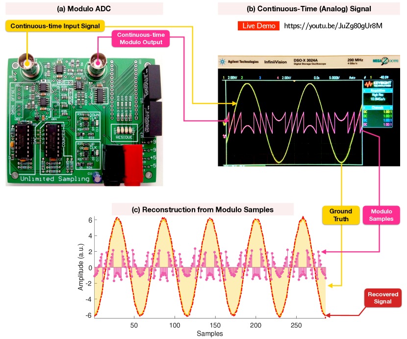
Thus, the USF addresses a major bottleneck in physical sensors by allowing the recovery of inputs beyond the sensor dynamic range. A first validation of the USF with experiments based on a modulo ADC were presented in [13]. In particular, it was shown that signals as large as can be recovered in a laboratory setup. The full sampling and reconstruction pipeline for the USF is shown in Fig. 1.
The initial works based on USF tackled signals supported on the real line spanned in a bandlimited [11, 12] or spline spaces [19]. There are also methods to recover signals with compressive priors [20, 21] and using wavelet filters [22]. Further extensions of the USF include compactly supported inputs [13], sparse signals [23] and also new acquisition models [14].
A new acquisition model called modulo-hysteresis was introduced in [24] and further discussed in [14], which considers hardware non-idealities and enables new recovery guarantees. The modulo-hysteresis was also implemented in a hardware prototype [14]. This line of work also paved the path to novel and exciting low-power acquisition neuromorphic applications [24, 25].
The methods discussed so far assume that the input is one-dimensional . However, in many applications, such as photography [19], X-ray imaging or Computed Tomography [26], the input signal is multi-dimensional.
Motivation for a multi-dimensional model
There have been attempts to address multi-dimensional inputs with modulo architectures by rasterizing and processing the signal line-by-line in imaging [27, 19, 26] or for lattice sampling [28]. However, the existing modulo sampling approaches for multi-dimensional data are based on a one-dimensional modulo operator that is applied sequentially on the slices of a multi-dimensional input. This considers each slice a distinct signal, and does not exploit that they are all part of a multi-dimensional input. In other words, this modulo operation represents a separable transformation that does not exploit the multi-dimensional nature of the input. Furthermore, it is known that non-separable transformations represent much more powerful tools in analysing multi-dimensional data [29, 30].
We consider only the problem of input recovery for noisy inputs, distinct from that of input denoising, which was addressed before for modulo sampling [31, 32]. Methods such as USF recover the noise corrupted input samples while keeping the noise sequence intact. However, USF (Theorem 1) is fundamentally restricted to work with noise amplitudes smaller than the modulo threshold. When this requirement is not satisfied, the input recovery is heavily distorted. This limitation is carried over to the existing attempts to apply USF to multi-dimensional data.
Contributions
Here we present a modulo model that exploits the multi-dimensional structure of the data in the encoding process. Specifically, via multi-dimensional sampling in dimensions, we are able to dedicate a -dimensional subspace to deal with noise reduction, leaving dimension for estimating the modulo folds. Specifically, our contributions are below:
-
We introduce a generalized -dimensional modulo operator for sampling on a lattice.
-
We prove that the operator is well-defined and the folding discontinuities are located along directions given by the lattice vectors.
-
We provide recovery guarantees under noiseless assumption.
-
Under Gaussian noise assumption, we provide an upper bound on the recovery error probability that drops to for high enough sampling rates.
-
Using a numerical study we show that the proposed model offers significantly better noise robustness than USF.
Notation
For , denotes the fractional part of and is the floor function. For a set , is the indicator function and is the set closure. The set of real and integer numbers are and , respectively. Let and , and let the sets restricted to positive numbers be and . We denote by the empty set.
We use bold lowercase for vectors such as , assumed to be column vectors unless otherwise specified. Matrices are denoted by bold uppercase, e.g., . The element on line and column in matrix is denoted by . Unless specified otherwise, we use notation to denote a vector and to denote a vector . When used in the same context, denotes the last coordinates of such that . Similarly, we denote by a matrix containing the last columns of matrix . For two vectors we denote their inner product by , where is the complex-conjugate. Norm denotes the Euclidean norm for a vector and norm is defined as . We denote by the determinant of matrix . We denote by a matrix with on the main diagonal and otherwise.
For a function , and represent the and norms, respectively. We denote by the Fourier transform applied to , defined as
| (1) |
where and . The inverse Fourier transform is defined as
| (2) |
The support of sequence is denoted by and the support of a function is . For two multi-dimensional sequences , denotes the multi-dimensional inner product defined as . The coefficients for the forward finite difference of order are denoted by . Specifically, it is defined as , where is defined recursively as , where , .
We denote by the set of vectors defining a lattice where and , where denotes the sampling period across dimension . Without loss of generality, we assume that are versors, i.e., . The vectors are assumed linearly independent, and thus is invertible. Therefore, a function can be equivalently evaluated using Cartesian coordinates as or lattice coordinates as such that . Unless specified otherwise, , denote the samples of the input function on lattice such that . The dual lattice is defined as , where and .
The -dimensional Paley-Wiener space of bandwidth relative to lattice consists of functions such that
| (3) |
For the one-dimensional case , the lattice matrices reduce to the trivial case and reduces to the classical one-dimensional Paley-Wiener space .
For a random variable we denote by p.d.f. its probability density function. We denote by the normal distribution with mean and standard deviation . A random variable drawn from the Gaussian normal distribution is denoted as .
2 Modulo acquisition and recovery
2.1 Recovery from one-dimensional modulo data
The centered modulo with threshold is a function satisfying [12]
| (4) |
When applied to a one-dimensional function the modulo non-linearity generates values .
In analogy to Shannon-Nyquist sampling theory, the first recovery result in the Unlimited Sensing Framework (USF) utilized bandlimited inputs, namely, . In the noiseless scenario, the unlimited sampling theorem [11, 12] guarantees that the input of the ideal modulo encoder can be recovered from the output samples provided that the sampling period satisfies . Furthermore, reconstruction is also possible in the case of data corrupted by bounded noise if the following is true [12]
| (5) |
The recovery approach used in [11, 12] aims to reconstruct the residual function defined as . In other words, for the ideal modulo encoder the values of lie on an equally spaced grid with step . However, this is not true for non-ideal modulo encoders exhibiting phenomena such as hysteresis, leading to reconstruction distortions.
A generalized model of the modulo operator, called modulo-hysteresis, was introduced for the one-dimensional scenario [33, 34, 14]. Here, we generalize this model to multi-dimensional sampling. As in the one-dimensional case, we will show that modulo-hysteresis enables the separation of the folding times, which will be used in the recovery in Section 3, 4, and 5. We begin with the definition of the one-dimensional modulo-hysteresis.
Definition 1 (One-dimensional modulo-hysteresis).
The operator with threshold and hysteresis , where , generates a function for input , such that, for
| (6) |
where
-
•
,
-
•
,
-
•
and are the folding time and sign respectively, satisfying and
| (7) | ||||
Furthermore, for we have . Let be the sequence of folding times and signs computed via (7) for . Then we define .
A key property of the 1D modulo-hysteresis is the folding time separation [14, 33]
| (8) |
We note that the ideal modulo, which satisfies for does not guarantee any separation via (8). The reconstruction problem proposed aims to recover from . Furthermore, it was shown that this approach enables handling a number of modulo non-idealities [14, 35, 33, 24].
3 Multi-dimensional modulo sampling
3.1 Multi-dimensional lattice sampling preliminaries
Let be a -dimensional scalar function. The data is then sampled on a lattice . We denote the resulting samples by . We assume that has a Fourier transform satisfying
Upon sampling, the spectrum of is copied periodically, to produce the multi-dimensional discrete-time Fourier transform , whose support satisfies
| (9) |
It was shown that can be recovered from its lattice samples if [36, 37]
| (10) |
To ensure that recovery is possible, we assume that the spectrum of has a compact support satisfying . Formally, our assumption is . Then can be reconstructed from samples if (10) is satisfied, which is sufficiently guaranteed if we replace by , for which the terms on the left-hand-side of (10) are computed as
| (11) |
We use that , yielding
| (12) | ||||
| (13) |
Therefore, (10) is true if
| (14) |
Just as in the one-dimensional case, considering the problem of sensor saturation motivates using the concept of modulo folding also in the multi-dimensional case. Next we go through some of the attempts to apply modulo for multi-dimensional data.
3.2 Previous approaches for recovery from multi-dimensional data
As in the one-dimensional case, the problem with computing directly is that the sample values may be very large which would saturate an analog-to-digital (ADC) acquisition device, which has a restricted dynamic range [12]. The modulo operator was applied previously for multi-dimensional inputs by processing a 1D slice at a time [19, 28]. However, these methods are not truly multi-dimensional because they don’t exploit the multi-dimensional structure of the data. Furthermore, when dealing with noise in 1D, the modulo samples require the separation of both residual and within the same dimension. This turns out to be contradictory, as detecting requires a high-pass filter (such as in the case of USF), while denoising is typically done with low-pass filters [34]. Furthermore, a denoising approach on modulo data was tested for multi-dimensional signals [31]. However, we center our analysis on purely modulo inversion techniques, where the noise sequence remains unaltered.
We define the following functions, representing slices of function . Let . Let denote the slice along dimension defined as . In the next proposition we also use a generic slices defined as the one-dimensional function by fixing dimensions . The following proposition was proven in [28].
Proposition 1 (Bandlimited slices).
The function satisfies . Furthermore, , .
Proof.
The proof is in Section 7.1. ∎
The proposition above proves that any slice of the multi-dimensional function along lattice dimension has the spectrum compactly supported within . Furthermore, this implies that a Bernšteĭn bound can be applied for each variable such that
| (15) | ||||
The works in [19] and [28] apply one-dimensional ideal modulo to :
Therefore we can define the "folded" multi-dimensional function as
| (16) |
where . Subsequently, the output samples are , where .
Then, recovering for all from represents a line-by-line approach used in [19, 26, 28], which is guaranteed to work if (5) holds true. However, as explained previously, this approach does not exploit the multi-dimensional structure of the input data. This is further motivated by the accepted knowledge in image processing that non-separability in multiple dimensions has a lot more to offer than separability [29, 30]. This motivates introducing a multi-dimensional modulo-hysteresis model in the next section. We will show that the new model allows a significantly large amount of noise, which is not possible with USF that processes the data line-by-line.
3.3 Towards multi-dimensional modulo-hysteresis acquisition
Inspired from the 1D modulo-hysteresis operator that showed improvements for noise robustness [34], we define in the following a new operator called multi-dimensional modulo-hysteresis that addresses the issues discussed in the previous subsection. The idea is to split the domain in disjoint sets confined in polytopes defined as
| (17) |
where and is the polytope edge length along directions parallel with versors . The set is created via the last vectors of the lattice basis where the basis coordinates lie in a set of rectangular polytopes such that , where
| (18) |
Note that . Sets thus can be used to split the domain of function in disjoint bands of width given by identified using the indices in , such that . By exploiting the smoothness of we can derive that, for a fixed , has bounded variation within each band, and thus the folding can occur simultaneously on all coordinates , which gives the folded signal a particular structure to be exploited in recovery. The definition of the new operator is given as follows.
Definition 2 (Multi-dimensional modulo-hysteresis).
The operator with threshold and hysteresis , where , generates a function for input such that, for
| (19) |
where denotes the modulo-hysteresis residual defined as
| (20) |
where satisfies (18), , , and satisfies
| (21) |
and are the folding times and signs in band , respectively, defined as
| (22) | |||
| (23) | |||
| (24) |
where , is a recursive sequence of functions for computing the residual such that , and . Furthermore satisfies
| (25) |
Furthermore, for we have
where . Let be the folding times and signs computed via (22), (23) for . Then we define .
We note that the operator in Definition 2 is backwards compatible with the one-dimensional operator in Definition 1. Specifically, if one chooses to be a single point instead of a hypercube, then and in (22) are the same as in Definition 1. Furthermore, it was shown that, for , the one-dimensional modulo-hysteresis operator in Definition 1 is identical to an ideal modulo operator (4) [14].
 |
||||
|
3.4 Properties of the proposed operator
In the following we give a number of properties of the multi-dimensional modulo-hysteresis operator for a bandlimited input.
Proposition 2 (Folding time separation).
Assume that are well-defined in (22) for and where and . Furthermore, assume that , where
| (26) |
Then
| (27) |
Proof.
The proof is in Section 7.1. ∎
Proposition 3 (Well-defined operator).
Proof.
The proof is in Section 7.1. ∎
Proposition 4 (Modulo output dynamic range).
Proof.
The proof is in Section 7.1. ∎
Proposition 4 shows that operator has a similar effect as the one-dimensional modulo nonlinearity, in that it keeps a signal within a fixed dynamic range .
Corollary 1 (Bound for intra-band variation).
The quantity defined in Proposition 27 can be bounded as
| (28) |
Proof.
The proof is in Section 7.1. ∎
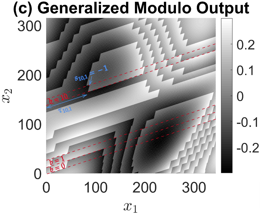
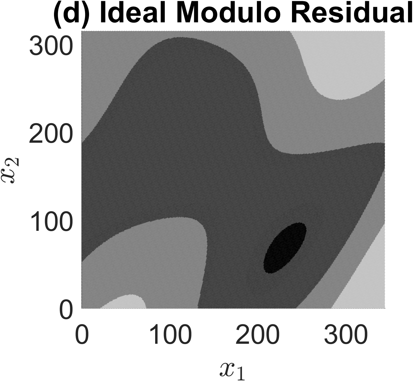
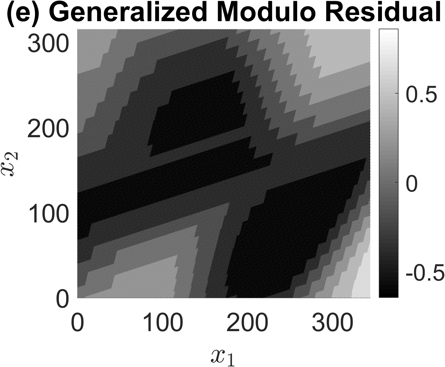
In Fig. 2 the variation of , which can be seen as folds along coordinates for , is gradual, meaning that changes by between neighboring bands. Formally, we define by the set comprising all neighboring bands of band below.
Definition 3 (Neighboring bands).
The set of vectors neighboring is defined as the set of all for which such that and .
In the following, we provide conditions for which where .
Proposition 5 (Variation of ).
For , let . Let and be the modulo-hysteresis constants for an input satisfying the following condition as per Definition 2
| (29) |
Then .
Proof.
We first note that sets and are neighboring polytopes which, via their definition, satisfy . Using this in conjunction with the properties of supremum and infimum, we get
| (30) |
Condition (29) implies due to Corollary 1. Therefore,
| (31) |
| (32) |
Given that, by definition, , it can be shown by direct derivation that . Furthermore, by swapping and in the derivation above we get
| (33) |
∎
Therefore, using Definition 2, for , in neighboring bands and the residual is either the same, or differs by . This is similar to the behavior of the residual around a folding time along dimension .
3.5 Problem formulation
The measurements are assumed to be samples on a multi-dimensional lattice , such that
| (34) |
where , and . The known variables are the input bandwidth , number of dimensions , the lattice , modulo-hysteresis parameters and output samples . The proposed reconstruction problem is to compute the input lattice samples defined as
| (35) |
where is an unknown integer. The input can only be reconstructed up to an integer multiple of given that (19,20).
4 Detecting modulo-hysteresis discontinuities
We define . For simplicity, we assume that , i.e., for a polytope we have an integer number of sampling periods along each of its edges of length and direction . The recovery is achieved in several steps
-
1.
Compute , the folding times and signs in each band .
-
2.
Compute residual (20).
-
3.
Compute the samples .
For step 1, we define a filter and compute . For detecting the folding times and signs, we choose , which is centered in sample along dimension in band as
| (36) |
where and is the number of samples in each band for fixed. For fixed , is a finite difference filter along dimension .
For detecting the , we need a filter detecting the change in for two bands , , such that and . We define as
| (37) |
where and is the number of samples in each band for , fixed. Therefore, similar to , filter is a finite difference filter along dimension which is perpendicular to the hyperplane separating bands and . Furthermore, is constant within each band and . This means that the finite difference filter is repeated times across dimensions , which has a noise averaging effect.
4.1 Detecting folding times and signs
To detect and , we use filter to compute sequence
| (38) |
In (38) the filtered samples are composed of three terms: the input term , the residual term and the noise term . Given that all three are unknown, the general recovery strategy is to separate them via thresholding; as will be shown later, thresholding samples allows to compute the folding times and signs. While this will be derived rigorously later in propositions 6 and 7, here we give a brief intuitive explanation of the recovery method, by explaining the effect that filter has on all terms in the right-hand-side of (38). A similar analysis applies to filter which will be described in Section 4.2.
As noted before, is a finite difference filter along dimension . It was shown for the one-dimensional case that this causes to vanish for large . Furthermore, it generates peaks at the folding times in residual and also amplifies the noise [12, 14]. This latter effect is undesirable for recovery. To decrease the effect of the noise the finite difference filter was convolved with a spline in the one-dimensional case, but this also makes the detection of more difficult [34]. Here we can address noise filtering without affecting the folding time detection by exploiting the multi-dimensional structure of .
For fixed , the filter is constant along dimensions as long as and thus the inner product has an averaging effect. However, we know that the modulo residual corresponding to is also constant within by definition, and therefore the averaging effect does not affect the residual edges, which are along dimension . Moreover, given that is smooth and changes slowly within a band , the filter averaging along dimensions has very little effect on . Therefore, along dimensions , the filter acts mainly on the noise sequence by narrowing its p.d.f. around the origin such that its effect gradually vanishes.
As in the one-dimensional case, the modulo output is smooth in-between the folds, and has discontinuities at the folding times. The filter responds with pulses of non-zero support to the input discontinuities. To account for this, we define by the support of the filtered residual such that (see [14] for details)
The following theorem shows how can be recovered by thresholding sequence , which is an important step in computing folding times .
Proposition 6 (Detection of folding times).
Let and let be the output of a multi-dimensional modulo-hysteresis model with parameters . Furthermore, let be the samples of the modulo output computed on lattice corrupted by a noise sequence . Furthermore, assume that and that
| (39) | ||||
If then with probability where
| (40) |
Proof.
The proof is in Section 7.2. ∎
Due to Proposition 6, for satisfying (39) and a fixed , one can choose such that the truth value of is evaluated correctly with an arbitrarily large probability. We note that measures the probability when a recovery error is possible, but not guaranteed, therefore the error probability is smaller in a real scenario. A small error in Proposition 6 means a large , which can be achieved by decreasing the sampling periods or increasing or number of dimensions .
The residual , used for reconstructing , requires detecting constants in addition to the folding times and signs , as will be explained in the next subsection.
4.2 Detecting constants
Given that we can only recover up to an integer multiple of (35), we define , where is the null vector of , and recover . Just as the folding times, different values of for adjacent bands cause discontinuities. However, unlike the detection of the folding times, here we have additional information. Specifically, we know that the discontinuities may only be located at the neighboring sides of polytopes . We use the filter (37) to detect the discontinuities in a similar fashion to detecting the folding times via . This time, however, the finite differences computed via evaluate variations across dimensions .
Proposition 7 (Detection of constants ).
Let , where and is the output of a modulo-hysteresis operator with parameters and satisfying
| (41) |
Furthermore, let , and such that . Assume that
| (42) | |||
| (43) |
Then the following is true with probability
| (44) |
where
| (45) |
Proof.
The proof is in Section 7.2. ∎
5 Input reconstruction
5.1 Recovery with the proposed operator
We begin with the noiseless input recovery scenario where, via Proposition 6, the set is perfectly identified with probability . Furthermore, a constant can be perfectly recovered from where according to Proposition 7. The following theorem proves the input recovery conditions in the case .
Theorem 2 (Noiseless input reconstruction).
Let and let be the output of a multi-dimensional modulo-hysteresis model with parameters . Furthermore, let be the samples of the modulo output computed on lattice . Furthermore, for , assume that
| (46) | |||
| (47) | |||
| (48) | |||
| (49) |
Then samples can be perfectly reconstructed from .
Proof.
The proof is in Section 7.2. ∎
The interpretation of the sufficient conditions in Theorem 2 is as follows. The modulo-hysteresis is well-defined due to a bounded intra-band variation guaranteed by (46). Condition (47) bounds the -th order difference of the input along all of the dimensions, ensuring that the filter has enough shrinking effect on the input. Finally, (48) and (49) guarantee enough samples in between the folds (48) and within each band (49) so that the supports of the filters detecting consecutive discontinuities don’t overlap.
In the general case where the following result holds true.
Theorem 3 (Noisy input reconstruction).
Proof.
Theorem 2 assumes that Proposition 6 and 7 hold with for all filters and . To calculate the overall error probability when this assumption is not true, we count the filters above, when used in reconstruction, as follows. There are a total of bands, and samples along dimension . Then the probability that Proposition 6 holds for all filters is .
Next, in the case of Proposition 7, we bound the error probability as follows
| (50) |
We note that we do not use all filters . Given that we use a set of samples that is contiguous along all dimensions, any band containing samples has at least one neighboring band that contains samples. Then, each constant can be computed using a single evaluation of , which, in total, is evaluated times, and the theorem follows. ∎
5.2 Comparison to ideal modulo recovery with Gaussian noise measurements
The USF was not analysed in the presence of Gaussian noise, but rather on bounded noise [12, 28]. However, USF can still be applied for recovery in the context of Gaussian noise, and the reconstruction would still be accurate in the instances when the noise sample with maximum amplitude satisfies the USF conditions. The modulo operator with Gaussian noise was considered before, but the main objective was denoising, rather than input reconstruction [32, 31]. In order to assess the advantage of the new operator, we provide some insight on reconstruction via USF for multi-dimensional inputs. Specifically, we note that, for an input and a lattice , the ideal modulo output is decomposed as (see also Section 2.1)
The recovery method from [28] involves a line-by-line approach, meaning that the recovery is performed along dimension , . By defining , , , , and , the recovery is performed by computing
| (51) | ||||
We remark that the processing in (51) is equivalent to applying filter (36) in the case of the multidimensional modulo-hysteresis operator when there is only one sample per band in all dimensions, i.e., . Even though the noise here is not bounded, we can derive the condition when the USF would work for a specific noise instance, which is [12]
for all . Thus, recovery is only guaranteed if the noise instance is bounded by
| (52) |
In a similar fashion to the derivation of (98) it can be shown that . We remark that the standard deviation of is always at least . Therefore, depending on the values of and , the probability that (52) holds may be very low. Conversely, in the recovery with the proposed operator , satisfies (98), where the standard deviation can be made arbitrarily small by increasing the number of samples within each band . In Section 6 this fact will be exploited to achieve significantly higher recovery performance for the proposed operator compared to ideal modulo .
6 Numerical study
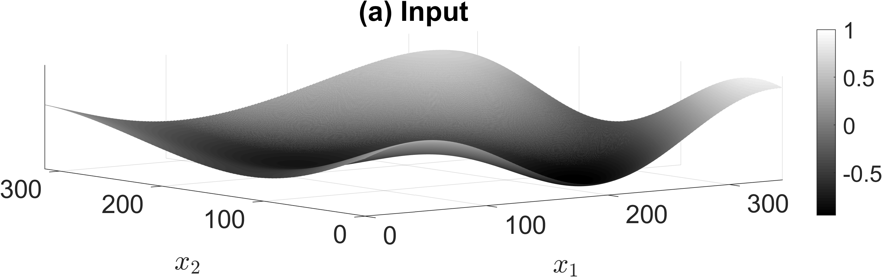
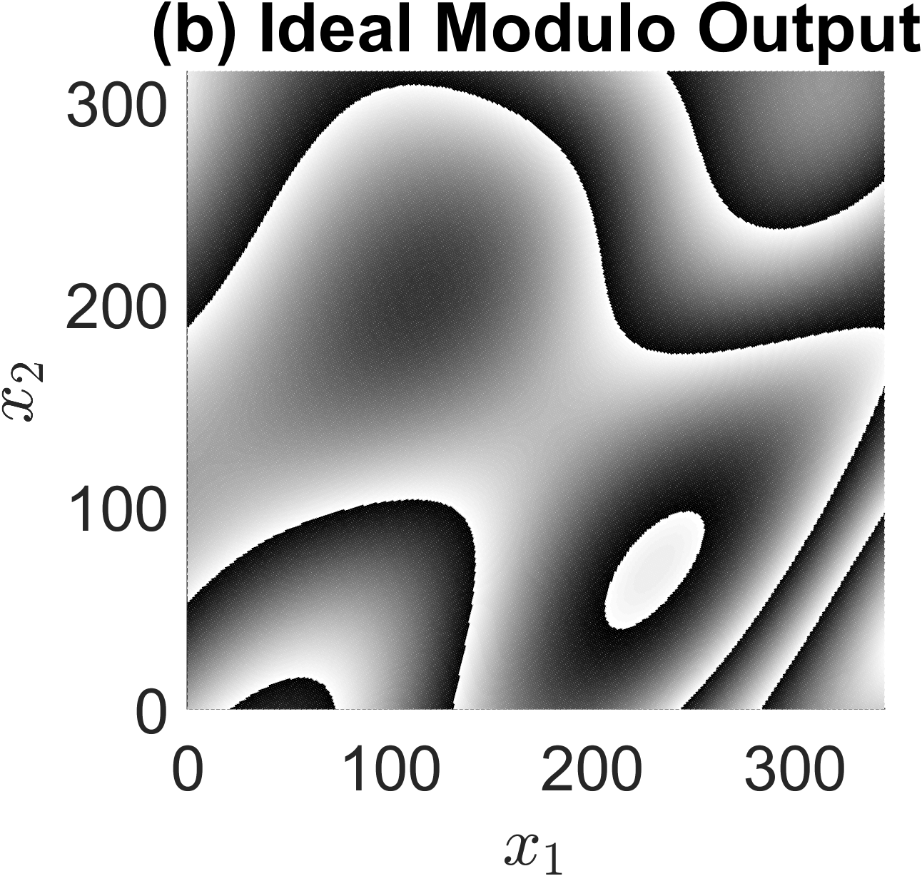
Let be a randomly generated matrix such that . The input was restricted to two variables for visualisation purposes, and was generated as , where
| (53) |

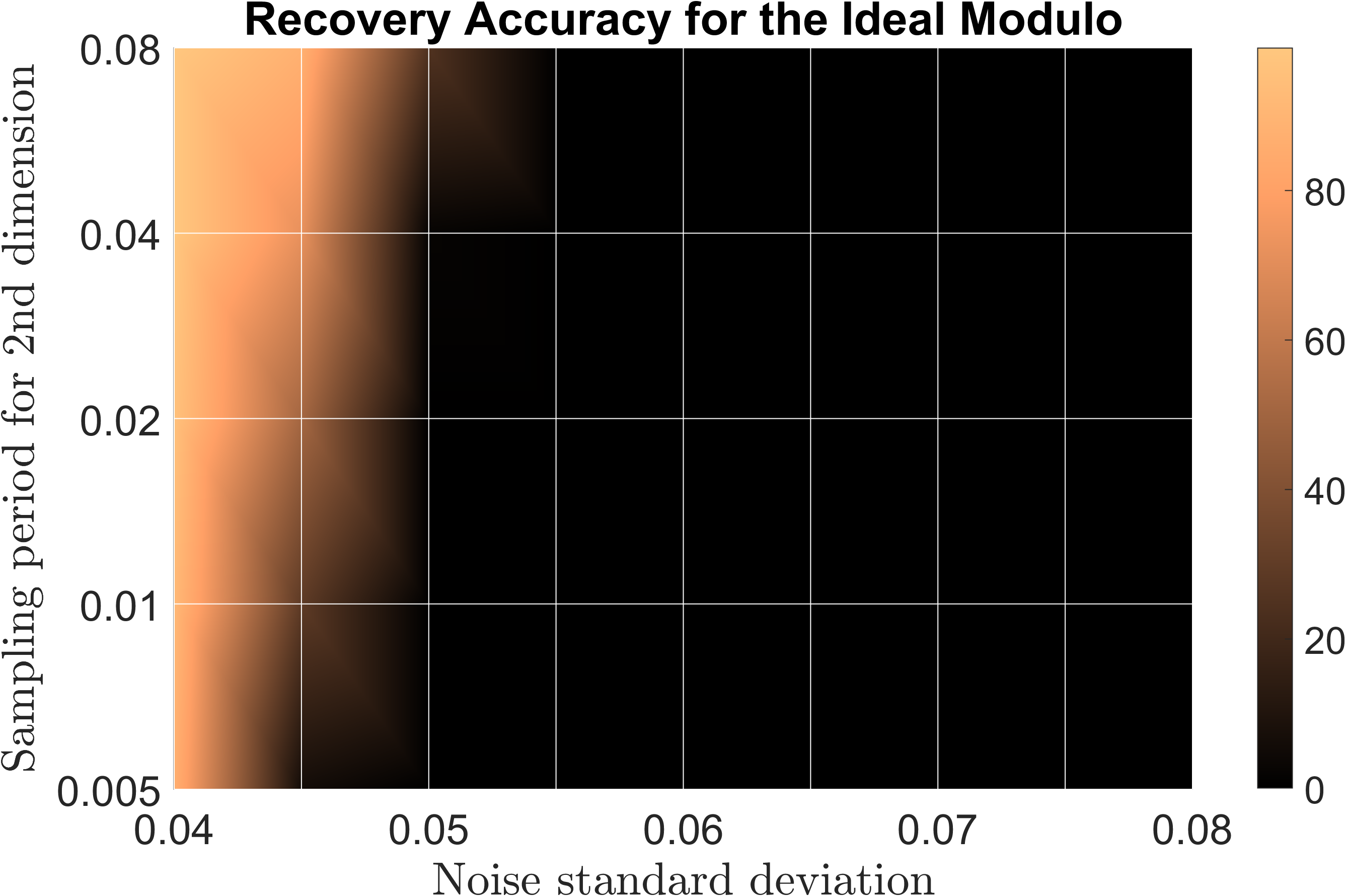
We selected , and computed for . The coefficients were randomly generated for , drawn from the uniform distribution on . The dynamic range of is . We encoded using the ideal modulo with threshold and the proposed modulo-hysteresis with . The output samples, computed on lattice with basis vectors and sampling periods . We kept constant because its choice affects in a similar fashion recovery from and (see [14]). We varied in the range . The output samples are
| (54) | |||
| (55) |
where . We varied in the range , and recovered the input up to a constant multiple of for and for . We generated random inputs and noise sequences and counted the number of inputs correctly reconstructed using each method. In our context, correctly reconstructed means that the recovery conditions hold true. The results are depicted in Fig. 3. We note that, while the accuracy increases significantly for for small , as proven by Theorem 3, for the reverse happens. This is because processes the input in a line-by-line fashion, and does not exploit in any way the higher resolution along dimension . In fact, here a higher resolution simply adds more noise samples from sequence , which are not filtered and thus increase the probability that (52) does not hold. We also note that, for larger sampling periods , performs slightly better for low noise, i.e., . This is explained by the fact that the modulo-hysteresis requirement is more strict than (52) given that . This is a small trade-off that enables to handle arbitrarily large values of for small enough sampling periods .
7 Proofs
7.1 Multi-Dimensional Modulo Properties
Proof for Proposition 1 (Bandlimited slices).
We consider the slice along dimension , with fixed. To this end, we apply the – dimensional inverse Fourier transform to corresponding to all variables apart from , such that
| (56) | ||||
| (57) | ||||
| (58) |
Therefore, the spectrum of depends on the spectrum of , which will be evaluated in the following. To this end, via the change of variable , we get that
| (59) | ||||
Using we get that . Then, via (59), we have that , and therefore in (56). It follows that , . Furthermore, choosing gives us , which finalizes the proof. ∎
Proof for Proposition 27 (Folding time separation).
We first show an intermediate result in the following lemma.
Lemma 1.
For a fixed vector indicating the modulo band and , let and be two functions defined as
| (60) | ||||
| (61) |
Then and are Lipschitz-continuous as functions of and is Lipschitz-continuous as function of . Furthermore, the Lipschitz constant in all cases is .
Proof.
We begin by deriving a bound for the Lischitz constant of function . Given that is differentiable, according to the mean value theorem
| (62) |
where is an intermediate point on the segment joining and . Due to the Cauchy-Schwartz inequality
| (63) |
Next, we use the Bernšteĭn bounds in (15) to derive a bound for as follows
| (64) |
which means is a Lipschitz-continuous function satisfying
| (65) |
For all and we have , which implies
| (66) | ||||
The final step is to show that is also Lipschitz, i.e., that the supremum does not change the Lipschitz constant. To this end, we note the following two properties of the supremum. Specifically, for and , such that
| (67) |
We derive that . Similarly, we get . Finally, we restrict in (67) to satisfy and select in (66) as , which yields
Taking above proves the required result. ∎
We begin by evaluating
| (68) |
Using that we derive
| (69) | ||||
Then, given that
we get . Furthermore, is Lipschitz-continuous due to Lemma 1, and therefore continuous. Thus, given that is true by definition, we get .
We then investigate the variation of function between folding times and as follows. Using Lemma 1, we get
and then we use that and to derive
Therefore the folding times satisfy the following bound
| (70) |
We note the resemblance between (70) the one-dimensional case (8). Next, we will show by induction that and then holds where sequence is computed according to (22). The base case is shown in the derivation to (70). For the induction step we proceed with computing .
| (71) | |||
| (72) | |||
| (73) |
We have that , which leads to two possible cases
-
1.
Next, we evaluate the sign of as follows
(75) (76) (77) The final inequality follows from the assumption . It follows that (74)
(78) -
2.
. As before, here we prove that , , and finally which leads to (78).
As in the base case , given that is true by definition and using the continuity of , we get . Using (78) and the same reasoning as in the base case leading to (70) the proposition follows. ∎
Proof for Proposition 3 (Well-defined operator).
For this to be true we need to show the existence of in (25). First, we derive some preliminary properties of . Due to Proposition 1 we have that and implicitly . Using the properties of the space and , it follows that
| (79) |
We require to show that the limit in (79) is uniform for all , which is done in the following lemma.
Lemma 2 (Uniform convergence).
The following holds true
Proof.
We prove by contradiction. Thus we assume
We select which leads to
| (80) |
We use that, because is bounded, then any sequence has a subsequence that converges to a point in the closure of , i.e.,
We then select in (80) and get
Furthermore, is a Lipschitz-continuous function with constant as shown in (65), which implies that
This allows defining the following lower bound on
We know that and . Then it follows that cannot converge to for , which directly contradicts (79). Then the starting assumption is wrong, and the Lemma follows. ∎
We approach this proof by contradiction. If we assume that does not exist it follows that in (22) is well-defined for . Given that, by definition, is increasing as a function of , then due to Proposition 27 it follows that . We use Lemma 2 for , which yields such that . Given our assumption on then such that . Thus, by definition, . Using (73)–(78) where is replaced by and functions are defined in (60),(61), one can show that . The next folding time satisfies . In the following we will show this is not possible. Specifically, for ,
We conclude that the definition of via (22) is therefore not possible, and thus our assumption that is well-defined for is false, and the proposition follows. ∎
Proof for Proposition 4 (Modulo output dynamic range).
We first assume that satisfies and then extrapolate to the whole real axis. Given the definition of function (24) it follows that and thus
It was shown before that (78). Furthermore, due to the definition of (22) we get that and when our assumption holds. By repeating the process above for we get . For , the process above is reproduced for . ∎
Proof for Corollary 1 (Bound for intra-band variation).
Let . As shown before (65), is a Lipschitz-continuous function with constant . Then it follows that
| (81) | ||||
| (82) |
We recall that satisfies (26)
| (83) |
We fix a , and define as
| (84) |
We then use the property that there always exists a sequence in a set converging to the infimum or supremum. Therefore, such that
| (85) |
Given that converges to the supremum and to the infimum, it follows that such that . Then
| (86) | ||||
| (87) |
By taking above we have that , and computing leads to the desired bound. ∎
7.2 Multi-Dimensional Modulo Recovery
Proof for Proposition 6 (Detection of folding times).
As in the continuous-time scenario, we denote the one-dimensional slices of the samples in each band by
| (88) | ||||
| (89) | ||||
| (90) |
where and . We note that, due to Definition 2, does not change with as long as . The filtered samples satisfy
We first exploit that where is bandlimited to , which yields [12, 14]
| (91) | ||||
Similarly, for the residual samples the following holds
| (92) | ||||
for all satisfying , given that does not change within the band as a function of (24). We note that and derive that
| (93) |
Therefore, if and , then, ,
| (94) | ||||
Furthermore, for , we get . Then, we identify if by thresholding sequence via the following inequalities.
| (95) |
Sequence is drawn from the normal distribution and is not bounded, therefore we can only guarantee that holds with a given probability. However, we will show that modulo-hysteresis allows increasing this probability exponentially.
We use two properties of the p.d.f. of Gaussian distributions. First, given random variables their summation satisfies , where . Second, for a random variable , the multiplication with a constant yields .
Then the noise term satisfies
| (96) | ||||
Using the two p.d.f. properties above, . As expected, averaging gradually narrows down the p.d.f. of the distribution around the origin. Furthermore, we can write
| (97) |
Given that , we will compute recursively the p.d.f. of as follows. First, . Given that , we get . Recursively,
| (98) |
In the equation above one can notice that the finite difference degree leads to an exponential increase in the standard deviation of the noise term. A very similar result was reported for bounded noise in the one-dimensional case [12, 14, 34]. However, in this multi-dimensional case we have the option to decrease the noise by increasing the number of samples . This can be done either by increasing the band size within the allowable range ensuring , but also by decreasing the sampling periods . Both of these act only on dimensions and are fully independent of dimension .
Therefore, the noise term in (38) represents a random variable that allows to correctly evaluate if via (95) when . The probability that this doesn’t hold is denoted by which is calculated using the p.d.f. of the normal distribution as
| (99) |
where and . The integral above can be bounded in terms of the complementary error function as follows, which finalizes the proof [38, 39]
| (100) |
∎
Proof for Proposition 7 (Detection of constants ).
We define by the samples filtered with where , such that and
Along the same lines as (91), we derive
| (101) |
Along dimension and for , the support of is
Furthermore, the discontinuity between the bands would be located in between the samples . Using the same reasoning as before (92-93)
| (102) |
Therefore, if and , then, , as before, we get (94)
Therefore, as before (95), we identify if by thresholding sequence via the following inequalities:
| (103) |
Assuming that , we compute as follows. We first show that
| (104) |
If we assume by contradiction that we get . However, from (102)-(103) we have that and . Given our assumption that the two quantities have the same sign, we get a contradiction and thus (104) is true.
Proof for Theorem 2 (Noiseless input recovery).
We note that, for , the results in Proposition 6 and 7 hold true with probability . We then compute using Proposition 7 as follows. Given that by definition, one can compute successively from for and subsequently from for . Repeating the process for yields .
To compute the folding times via Proposition 6, we require that the sets characterized by each folding time in do not overlap. Specifically we require that
for . A sufficient condition for this is
| (108) |
which can be guaranteed via Proposition 27 if
| (109) |
Without reducing the generality we first assume that and thus . As before, the case is treated as a mirrored version of . An immediate consequence of (108) is that for . Because there is no actual jump taking place at and via Proposition 6. The smallest for which filtered output satisfies is . The last index corresponding to folding time detected via is . We can compute and as
| (110) | ||||
| (111) |
Assuming (109) to be true, one can then compute recursively sequences corresponding to folding time as follows
| (112) | ||||
| (113) |
The folding time is estimated as . As in the case we can show that . Therefore . Even though the folding time is not perfectly computed, this has no effect on the input recovery because and we only evaluate the residual at the sampling locations . This means that replacing by in the expression of yields the same values (see Definition 2)
| (114) | ||||
We note that, as explained before, we do not recover but . This will be accounted for at the final input reconstruction stage.
Furthermore, we estimate the sign as . We will show that as follows. Given that and , then, via (38), it follows that
We use the fact that does not change for . For , using the expression of and (114),
| (115) | ||||
By applying the change of variable
| (116) | ||||
| (117) |
The last equality can be shown recursively via direct calculation for , given that , which proves that .
After the folding times and signs are computed as above for all , the input samples are reconstructed as
| (118) |
where , which leads to . ∎
8 Conclusion
The Unlimited Sampling Framework (USF) provides sampling rate guarantees that allow tackling high dynamic range signals in the one-dimensional case. For multi-dimensional signals, USF is typically applied sequentially, thus not exploiting the multi-dimensional structure of the input. In this paper, we
-
•
introduced the first multi-dimensional modulo operator and associated input reconstruction method from lattice samples,
-
•
derived sampling rate conditions under which the reconstruction is perfect in the noiseless scenario,
-
•
provided probability error bounds under Gaussian noise assumption,
-
•
showed numerically that, while USF does not allow noise amplitudes larger than the modulo threshold, the proposed approach allows arbitrarily high noise for sufficiently small sampling times.
This work can be extended in a number of ways
-
1.
It can be coupled with modulo denoising approaches such as [31] to yield enhanced reconstruction algorithms.
-
2.
While it is assumed that the input is bandlimited, this work can be extended for inputs generated with B-splines or sparse inputs.
- 3.
- 4.
-
5.
The current line of work can lead to a the implementation of a new multi-dimensional hardware prototype.
References
- [1] R. M. Gray, D. L. Neuhoff, Quantization, IEEE Trans. Inf. Theory 44 (6) (1998) 2325–2383. doi:10.1109/18.720541.
- [2] W. Sun, X. Zhou, Reconstruction of band-limited functions from local averages, Constructive Approximation 18 (2) (2002) 205–222. doi:10.1007/s00365-001-0011-y.
- [3] D. L. Donoho, I. M. Johnstone, Ideal spatial adaptation by wavelet shrinkage, Biometrika 81 (3) (1994) 425–455. doi:10.1093/biomet/81.3.425.
- [4] T. Blumensath, M. E. Davies, Iterative hard thresholding for compressed sensing, Applied and Computational Harmonic Analysis 27 (3) (2009) 265–274. doi:10.1016/j.acha.2009.04.002.
- [5] B. Smith, Instantaneous companding of quantized signals, The Bell System Technical Journal 36 (3) (1957) 653–710. doi:10.1002/j.1538-7305.1957.tb03858.x.
-
[6]
P. Smaragdis, Dynamic range
extension using interleaved gains, IEEE Audio, Speech, Language Process.
17 (5) (2009) 966–973.
doi:10.1109/tasl.2008.2012322.
URL http://dx.doi.org/10.1109/TASL.2008.2012322 -
[7]
J. Abel, J. Smith,
Restoring a clipped
signal, in: IEEE Intl. Conf. on Acoustics, Speech and Sig. Proc.
(ICASSP), 1991.
doi:10.1109/icassp.1991.150655.
URL http://dx.doi.org/10.1109/icassp.1991.150655 -
[8]
J. Zhang, J. Hao, X. Zhao, S. Wang, L. Zhao, W. Wang, Z. Yao,
Restoration of clipped seismic
waveforms using projection onto convex sets method, Nature Sci. Rep. 6 (1).
doi:10.1038/srep39056.
URL https://doi.org/10.1038/srep39056 -
[9]
A. Adler, V. Emiya, M. G. Jafari, M. Elad, R. Gribonval, M. D. Plumbley,
Audio inpainting, IEEE
Trans. Acoust., Speech, Signal Process. 20 (3) (2012) 922–932.
doi:10.1109/tasl.2011.2168211.
URL https://doi.org/10.1109/tasl.2011.2168211 -
[10]
P. E. Debevec, J. Malik,
Recovering high dynamic range
radiance maps from photographs, in: ACM Siggraph, 1997.
doi:10.1145/258734.258884.
URL https://doi.org/10.1145/258734.258884 -
[11]
A. Bhandari, F. Krahmer, R. Raskar,
On unlimited sampling,
in: Intl. Conf. on Sampling Theory and Applications (SampTA), 2017, pp.
31–35.
doi:10.1109/sampta.2017.8024471.
URL https://doi.org/10.1109/sampta.2017.8024471 - [12] A. Bhandari, F. Krahmer, R. Raskar, On unlimited sampling and reconstruction, IEEE Trans. Sig. Proc. 69 (2020) 3827–3839. doi:10.1109/tsp.2020.3041955.
- [13] A. Bhandari, F. Krahmer, T. Poskitt, Unlimited sampling from theory to practice: Fourier-Prony recovery and prototype ADC, IEEE Trans. Sig. Proc. (2021) 1131–1141doi:10.1109/TSP.2021.3113497.
- [14] D. Florescu, F. Krahmer, A. Bhandari, The surprising benefits of hysteresis in unlimited sampling: Theory, algorithms and experiments, IEEE Trans. Sig. Proc. 70 (2022) 616–630. doi:10.1109/tsp.2022.3142507.
- [15] A. Bhandari, F. Krahmer, R. Raskar, Unlimited sampling of sparse signals, in: IEEE Intl. Conf. on Acoustics, Speech and Signal Processing (ICASSP), 2018, pp. 4569–4573. doi:10.1109/icassp.2018.8462231.
- [16] A. Bhandari, F. Krahmer, R. Raskar, Unlimited sampling of sparse sinusoidal mixtures, in: IEEE Intl. Sym. on Information Theory (ISIT), 2018, pp. 336–340. doi:10.1109/isit.2018.8437122.
- [17] A. Bhandari, F. Krahmer, On identifiability in unlimited sampling, in: Intl. Conf. on Sampling Theory and Applications (SampTA), 2019.
- [18] A. Bhandari, F. Krahmer, R. Raskar, Methods and apparatus for modulo sampling and recovery (May 2020).
- [19] A. Bhandari, F. Krahmer, HDR imaging from quantization noise, in: IEEE Intl. Conf. on Image Processing (ICIP), 2020, pp. 101–105. doi:10.1109/icip40778.2020.9190872.
- [20] V. Shah, C. Hegde, Signal reconstruction from modulo observations, in: 2019 IEEE Global Conference on Signal and Information Processing (GlobalSIP), IEEE, 2019, pp. 1–5.
- [21] O. Musa, P. Jung, N. Goertz, Generalized approximate message passing for unlimited sampling of sparse signals, in: IEEE Global Conf. on Signal and Information Proc., 2018, pp. 336–340.
- [22] S. Rudresh, A. Adiga, B. A. Shenoy, C. S. Seelamantula, Wavelet-based reconstruction for unlimited sampling, in: IEEE Intl. Conf. on Acoustics, Speech and Signal Processing (ICASSP), 2018, pp. 4584–4588.
- [23] A. Bhandari, Back in the US-SR: Unlimited sampling and sparse super-resolution with its hardware validation, IEEE Signal Process. Lett. 29 (2022) 1047 – 1051.
- [24] D. Florescu, F. Krahmer, A. Bhandari, Event-driven modulo sampling, in: IEEE Intl. Conf. on Acoustics, Speech and Signal Processing (ICASSP), 2021, pp. 5435–5439. doi:10.1109/icassp39728.2021.9414152.
- [25] D. Florescu, A. Bhandari, Modulo event-driven sampling: System identification and hardware experiments, in: IEEE Intl. Conf. on Acoustics, Speech and Signal Processing (ICASSP), 2022, pp. 5747–5751.
- [26] M. Beckmann, A. Bhandari, F. Krahmer, The modulo Radon transform: Theory, algorithms, and applications, SIAM Journal on Imaging Sciences 15 (2) (2022) 455–490. doi:10.1137/21m1424615.
- [27] S. Fernandez-Menduina, F. Krahmer, G. Leus, A. Bhandari, Computational array signal processing via modulo non-linearities, IEEE Trans. Sig. Proc. 70 (2022) 2168–2179.
- [28] V. Bouis, F. Krahmer, A. Bhandari, Multidimensional unlimited sampling: A geometrical perspective, in: European Sig. Proc. Conf. (EUSIPCO), 2020, pp. 2314–2318.
- [29] X. Zhao, J. Chen, M. Karczewicz, A. Said, V. Seregin, Joint separable and non-separable transforms for next-generation video coding, IEEE Trans. Image Proc. 27 (5) (2018) 2514–2525.
- [30] A. Cohen, I. Daubechies, Non-separable bidimensional wavelet bases, Revista Matematica Iberoamericana 9 (1) (1993) 51–137.
- [31] H. Tyagi, Error analysis for denoising smooth modulo signals on a graph, Applied and Computational Harmonic Analysis 57 (2022) 151–184.
- [32] M. Fanuel, H. Tyagi, Denoising modulo samples: k-nn regression and tightness of sdp relaxation, Information and Inference: A Journal of the IMA 11 (2) (2022) 637–677.
- [33] D. Florescu, A. Bhandari, Unlimited sampling with local averages, in: IEEE Intl. Conf. on Acoustics, Speech and Signal Processing (ICASSP), 2022, pp. 5742–5746.
- [34] D. Florescu, A. Bhandari, Unlimited sampling via generalized thresholding, in: IEEE Intl. Symp. on Information Theory (ISIT), 2022, pp. 1606–1611.
- [35] D. Florescu, F. Krahmer, A. Bhandari, Unlimited sampling with hysteresis, in: 55th Asilomar Conf. on Signals, Systems, and Computers, 2021, pp. 831–835. doi:10.1109/ieeeconf53345.2021.9723306.
- [36] E. Viscito, J. P. Allebach, The analysis and design of multidimensional FIR perfect reconstruction filter banks for arbitrary sampling lattices, IEEE Trans. Circuits Syst. 38 (1) (1991) 29–41.
- [37] Y. M. Lu, M. N. Do, R. S. Laugesen, A computable Fourier condition generating alias-free sampling lattices, IEEE Trans. Sig. Proc. 57 (5) (2009) 1768–1782.
- [38] M. Chiani, D. Dardari, M. K. Simon, New exponential bounds and approximations for the computation of error probability in fading channels, IEEE Trans. Wireless Commun. 2 (4) (2003) 840–845.
- [39] J. Wozencraft, I. M. Jacobs, Principles of communication engineering., Wiley, 1965.
- [40] G. Gallego, T. Delbrück, G. Orchard, C. Bartolozzi, B. Taba, A. Censi, S. Leutenegger, A. J. Davison, J. Conradt, K. Daniilidis, et al., Event-based vision: A survey, IEEE Trans. Pattern Anal. Mach. Intell. 44 (1) (2020) 154–180.
- [41] O. Graf, A. Bhandari, F. Krahmer, One-bit unlimited sampling, in: IEEE Intl. Conf. on Acoustics, Speech and Signal Processing (ICASSP), 2019, pp. 5102–5106.