Behavioral Theory for Stochastic Systems?
A Data-driven Journey from Willems to Wiener and Back Again

Abstract

The fundamental lemma by Jan C. Willems and co-workers is deeply rooted in behavioral systems theory and it has become one of the supporting pillars of the recent progress on data-driven control and system analysis. This tutorial-style paper combines recent insights into stochastic and descriptor-system formulations of the lemma to further extend and broaden the formal basis for behavioral theory of stochastic linear systems. We show that series expansions—in particular Polynomial Chaos Expansions (PCE) of $L^{2}$-random variables, which date back to Norbert Wiener’s seminal work—enable equivalent behavioral characterizations of linear stochastic systems. Specifically, we prove that under mild assumptions the behavior of the dynamics of the $L^{2}$-random variables is equivalent to the behavior of the dynamics of the series expansion coefficients and that it entails the behavior composed of sampled realization trajectories. We also illustrate the short-comings of the behavior associated to the time-evolution of the statistical moments. The paper culminates in the formulation of the stochastic fundamental lemma for linear time-invariant systems, which in turn enables numerically tractable formulations of data-driven stochastic optimal control combining Hankel matrices in realization data (i.e. in measurements) with PCE concepts.

1 Introduction — Spring has arrived

In popular culture winter is coming is an established meme. In the context of the past and infamous AI winter [AIw, 2005] and its effect on research addressing data-driven methods, the recent rapid increase of interest and available results evidences the opposite. That is, we are currently experiencing an ongoing extremely vibrant growth period of research activities on data-driven methods for systems and control at least partially catalyzed by AI.

From the control perspective, data-driven methods at large can be understood as an attempt to overcome the traditional two-step procedure of modeling—either first principles combined with parameter estimation or system identification based on measurement data—and subsequently designing a controller for the obtained system/process model, see Figure 1. Building on the success and impact of subspace identification methods [Verhaegen, 2015, Markovsky et al., 2006], a recent stream of papers—which, e.g., includes De Persis & Tesi [2019], Favoreel et al. [1999], Fiedler & Lucia [2021], van Waarde et al. [2022] and the tutorial survey Markovsky & Dörfler [2021]—has analyzed the so-called direct approach to control design, see Figure 1. This approach aims at obtaining a non-parametric system description directly from data, i.e. without identifying system matrices, and at the design of feedback laws directly using this description.

Figure 1: Direct and indirect approaches to data-driven controller design.

In turn, subspace identification techniques are closely linked to behavioral concepts in systems and control, which have been conceived by Jan C. Willems; see Willems [1986a, b, 1987] for original references, Polderman & Willems [1997], Markovsky et al. [2006] for textbook expositions, and Willems [2007] for an introduction. It stands to reason that behavioral systems theory is indeed foundational for a wide range of recent results on data-driven control [Markovsky, 2021, Markovsky & Dörfler, 2021].

The pivotal result in this context shows for controllable finite-dimensional Linear Time-Invariant (LTI) systems that all input-output-state trajectories of finite length lie in the column space of suitable Hankel matrices constructed directly from data. It appeared already in the seminal paper by Willems et al. [2005]—hence it is commonly referenced as the Fundamental Lemma of Willems’ et al. Given the recent and seemingly exponential growth of publications extending/tailoring the fundamental lemma to specific system classes and using it for data-driven control, we postpone a more detailed literature review with respect to the former to Section 2.2. With respect to the latter, we remark that the two most frequent usages of the fundamental lemma for control design are output-feedback predictive control and direct feedback design Markovsky & Dörfler [2021]. The major conceptual advantage of output-feedback predictive control is that it alleviates the need to design state estimators. The earliest conception of Model Predictive Control (MPC) based on Hankel matrices, which did not receive widespread attention, appears to be Yang & Li [2015]. This line of research bifurcated to exponential growth with Coulson et al. [2019a] and numerous follow-ups. With respect to data-driven feedback design, we refer to De Persis & Tesi [2019], Markovsky & Dörfler [2021] and the references therein. Both lines of research are linked by the concept of optimizing closed-loop behaviors, cf. Dörfler et al. [2022]. So far, applications of data-driven control based on behavioral concepts include power systems [Schmitz et al., 2022a, Huang et al., 2019, Carlet et al., 2020], autonomous driving [Wang et al., 2022], and building control [Lian et al., 2021, O’Dwyer et al., 2022, Bilgic et al., 2022].

Interestingly, the common scope of behavioral systems theory and its major success in data-driven control in discrete-time settings go along with the orthogonal trend of limited progress with respect to behavioral approaches for stochastic systems, cf. the open problems identified by Markovsky & Dörfler [2021]. The ultimate paper of Jan C. Willems discusses behavioral ideas for stochastic systems [Willems, 2013]. Therein the main focus is on open stochastic static systems, their interconnection, and the construction of appropriate $\sigma$-algebras. Baggio & Sepulchre [2017] extend this to a canonical kernel representation of stochastic LTI processes. Following a different route, Pola et al. [2015, 2016] use behavioral ideas to study equivalence concepts for stochastic linear systems in discrete-time and continuous-time settings without actually defining the stochastic behavior as such. This has been extended to descriptor systems, i.e. discrete-time LTI systems subject to linear algebraic constraints, by Pola [2017]. Yet, none of these works covers data-driven representations of stochastic LTI systems.

Moreover, several approaches to behavioral concepts in infinite-dimensional settings have proposed: Pillai & Willems [1999], Pillai & Shankar [1999] discuss behavioral kernel representations of systems with distributed parameters using an algebraic approach. This is extended to dissipative systems by Pillai & Willems [2002], while Yamamoto & Willems [2008] focus on controllability in a behavioral setting. Ball & Staffans [2006] discuss conservative realizations of linear systems on Hilbert spaces in a behavioral setting, while Seiler & Zerz [2015] give an overview on algebraic theory for linear systems. Arguably, data-driven control of infinite-dimensional systems would require measurement data in appropriate infinite-dimensional spaces. Likewise data-driven approaches to stochastic systems are seemingly limited in applicability as stochastic processes are typically described via cumulative distributions, probability densities, or random variables—all of which are, in general, infinite dimensional.

Statistical moments, i.e., expectation, co-variance, skewness etc., provide an alternative representation of random variables, which is finite dimensional under rather specific assumptions on the underlying distribution. One may claim that the frequently-used modeling in terms of the first two moments (expectation and co-variance) does not stretch far beyond i.i.d. (independent and identically distributed) Gaussian uncertainties as moment closures for nonlinear systems are difficult and as manifold applications require modeling non-Gaussian uncertainties. In turn, non-Gaussian random variables frequently induce the need for higher-order moments, see, e.g., [Kuehn, 2016, Singh & Hespanha, 2010]. Even in cases where expectation and co-variance capture sufficient information about the uncertainty, the fact that they parameterize random variables in nonlinear fashion—i.e., any scalar Gaussian is given as the sum of its mean and square root of the variance times a standard normal distribution—often complicates their use.

Remarkably, already in the 1930s Norbert Wiener’s most cited journal paper proposed an alternative avenue [Wiener, 1938]. Therein, Wiener suggested to represent random variables via series expansions expressed in suitable polynomial bases of the underlying probability space. The required structure is the Hilbert space of $L^{2}$-random variables, i.e., the linear function space equipped with an inner product which contains all random variables of finite variance. This approach is commonly denoted as Wiener chaos expansion, as polynomial chaos, or as generalized polynomial chaos. For the sake of brevity, we gloss here over the subtle distinctions of these methods. The obtained series are denoted as Polynomial Chaos Expansions (PCE). Importantly, PCEs and related expansions parameterize a large class of Gaussian and non-Gaussian random variables in a linear structure, while moments lead, in general, to nonlinear representations. Without any detailed elaboration, we remark that polynomial chaos approaches are established for uncertainty quantification and uncertainty propagation [O’Hagan, 2013, Sullivan, 2015]. Very often one leverages that the finiteness of the PCE is closely related to the appropriate choice of the basis, i.e., a suitable choice allows for a finite series expansion of non-Gaussian random variables [Xiu & Karniadakis, 2002, Mühlpfordt et al., 2018b]. PCEs have also seen widespread and continued use in systems and control, e.g., for system analysis [Nagy & Braatz, 2007, Kim et al., 2013, Ahbe et al., 2020], for stochastic MPC [Mesbah & Streif, 2015, Mesbah, 2016, Fagiano & Khammash, 2012], and for optimization in power systems [Mühlpfordt et al., 2017, 2018a].

Figure 2: Illustration of contents.

In light of the growing success of behavioral systems theory in data-driven control this paper moves towards behavioral and data-driven concepts for stochastic linear systems. Hence, it extends the scope of the earlier and excellent overview [Markovsky & Dörfler, 2021], which has explicitly called for further investigation of the stochastic setting. Moreover, Markovsky & Dörfler [2021] provide a detailed exposition on issues and remedies surrounding the use of data corrupted by measurement noise and on the estimation of missing data. Hence, we do not revisit these aspects here. Specifically, the outline of the present paper is as follows (see also Figure 2):

In Section 2 we recapitulate the deterministic fundamental lemma and we give a problem statement for stochastic systems. Moreover, we provide a concise overview on Willems-inspired fundamental-lemma type results. To support the further developments, Section 3 turns to model-based representations of stochastic dynamics, it recalls the basics of Wiener chaos expansions and PCE, and it revisits the co-variance propagation for LTI systems.

In Section 4 the insights of Willems and Wiener are combined to derive our main contributions, i.e., we discuss different behavioral characterizations of stochastic systems. We introduce the behavior of the dynamics of the series expansion coefficients (in short expansion coefficient behavior) before we turn to the behavior of the dynamics in random variables (in short random variable behavior) and to the behavior associated to the time-evolution of the statistical moments (in short moment behavior). We also introduce the concept of behavioral lifts, i.e., we characterize the underlying relations between the behaviors referring to expansion coefficients, to random variables, and to realizations. Moreover, we show why and how moment characterisations fall short in the behavioral context.

Section 5 then continues to data-driven representations via the fundamental lemma tailored to stochastic systems [Pan et al., 2022b] before the results are extended to stochastic descriptor systems in the subsequent section. The crucial observation, which carries over from Pan et al. [2022b], is that due to the behavioral lift the Hankel matrices can be constructed from measurements of realization data (or sampled/measured trajectories) while the PCE framework allows to capture random variables exactly.

We prove that, under rather mild assumptions, for discrete-time stochastic systems measurements of finite-dimensional realization data (i.e. sampled trajectories of finite length) suffice to characterize the evolution of stochastic input, state, and output variables via an appropriate image representation obtained in the fundamental lemma for stochastic systems. To put it in the words of Willems [2013], our findings support the viewpoint that

[in terms of behavioral systems theory and in terms of the fundamental lemma] deterministic systems emerge as special cases of stochastic systems, as they should,

which is also fully aligned with Baggio & Sepulchre [2017].

Section 6 discusses data-driven stochastic optimal control, i.e., the computation of optimal non-anticipatory policies. Further, model-based analysis is put into action to ensure causality of the obtained optimal solutions.

Section 7 transfers the obtained insights on the stochastic fundamental lemma and on data-driven stochastic optimal control to descriptor systems. While from a model-based viewpoint descriptor LTI representations are more general than explicit ones, from the behavioral perspective both are (modulo the choice of inputs and outputs) equivalent representation instances of linear time-invariant systems, cf. [Willems, 1986a, 2007]. We show that it is the causality requirement of stochastic optimal control that marks the watershed between descriptor and explicit LTI systems in data-driven settings. Put differently, in data-driven settings with underlying descriptor structures the computation of non-anticipatory control actions requires careful analysis.

Section 8 draws upon numerical examples to illustrate our findings. The paper closes with an outlook on open problems and conclusions in Sections 9 and 10.

Notation. The non-negative and the positive integers are denoted by $\mathds{N}$ and $\mathds{Z}_{+}$, respectively. For $n,m\in\mathds{N}$ with $n\leq m$ we define $\mathds{I}_{[n,m]}\doteq[n,m]\cap\mathds{N}$. For two sets $\Omega$ and $M$, $\Omega^{M}$ denotes the set of all mappings $f:M\rightarrow\Omega$. Further, for two sets $\Omega_{1}$ and $\Omega_{2}$, we identify the Cartesian product $\Omega_{1}^{M}\times\Omega_{2}^{M}$ with $(\Omega_{1}\times\Omega_{2})^{M}$. The restriction of a function $f\in\Omega^{M}$ to a subset $M_{0}\subset M$ is denoted by $f|_{M_{0}}$. In the case $M=\mathds{I}_{[n,m]}$ we use for $f\in\Omega^{M}$ the notation $f_{k}\doteq f(k)$ and, when there is no possibility of confusion, also $f^{k}=f(k)$ for $k\in M$. Moreover, for $f\in\Omega^{M}$, where $\Omega=\mathds{R}^{d}$ and $M\subset\mathds{N}$ such that $\mathds{I}_{[n,m]}\subset M$, we define $\mathbf{f}_{[n,m]}\doteq\begin{bmatrix}f_{n}^{\top}&\dots&f_{m}^{\top}\end{bmatrix}{}^{\top}$. The identity matrix and zero matrix are designated by $I_{n}$ and $0_{n\times m}$. For a matrix $A$ we use the notations $\operatorname{rk}(A)$, $\operatorname{colsp}(A)$, and $A^{\dagger}$ for the rank, the column span, and the Moore–Penrose inverse of $A$, respectively. The Kronecker product of two matrices $A$ and $B$ is denoted by $A\otimes B$.

2 Preliminaries and Problem Statement

We first recall some basic concepts of behavioral systems theory and briefly revisit the fundamental lemma. We refer the reader to Markovsky & Dörfler [2021] for a recent and much-more-detailed survey on behavioral systems theory and its use for data-driven control of deterministic systems. For readers familiar with this survey, the first subsection only sets the notation used hereafter. Then, we give a problem statement and point out upcoming novel results in the stochastic setting. Finally, we conclude this section with a concise overview of fundamental-lemma-type results.

From an abstract point of view, a system $\Sigma$ is a triplet $\Sigma=(\mathds{T},\mathds{W},\mathfrak{B})$ with time axis $\mathds{T}\subseteq\mathds{R}$, signal space $\mathds{W}$, and behavior $\mathfrak{B}\subseteq\mathds{W}^{\mathds{T}}$. Specifically, we consider linear time-invariant discrete-time dynamics represented by

$$x_{k+1} =Ax_{k}+Bu_{k}$$ (1a)

$$y_{k} =Cx_{k}+Du_{k},$$ (1b)

where $x_{k}\in\mathds{R}^{n_{x}}$, $u_{k}\in\mathds{R}^{n_{u}}$, and $y_{k}\in\mathds{R}^{n_{y}}$ are the state, the input, and the output at time instant $k\in\mathds{N}$, respectively. Further, we have $A\in\mathds{R}^{n_{x}\times n_{x}}$, $B\in\mathds{R}^{n_{x}\times n_{u}}$, $C\in\mathds{R}^{n_{y}\times n_{x}}$, and $D\in\mathds{R}^{n_{y}\times n_{u}}$. In this situation the time-axis is given by $\mathds{T}=\mathds{N}$, and the signal space by $\mathds{W}=\mathds{R}^{n_{x}+n_{u}+n_{y}}$ or, if only input and output variables are considered, by $\mathds{W}=\mathds{R}^{n_{u}+n_{y}}$.

Subsequently, we may occasionally deviate from the rigorous behavioral wording, that is whenever no confusion can arise we use the word system to refer to a system or to its representation in synonymous fashion. The dynamics (1) can be described in the language of behavioral systems theory advocated by Polderman & Willems [1997], see also Willems [1991], Markovsky et al. [2006]. The (full) behavior of system (1) is

$$\mathfrak{B}_{\infty}\doteq\left\{(x,u,y)\,\middle|\,\begin{gathered}x\in(\mathds{R}^{n_{x}})^{\mathds{N}},u\in(\mathds{R}^{n_{u}})^{\mathds{N}},y\in(\mathds{R}^{n_{y}})^{\mathds{N}}\\ (x_{k+1},x_{k},u_{k},y_{k})\text{ satisfies \eqref{sys} }\forall k\in\mathds{N}\end{gathered}\right\}$$ (2)

which contains all state-input-output trajectories of (1). The trajectories of finite horizon $T\in\mathds{N}$ are collected in the finite-horizon behavior

$$\mathfrak{B}_{T}=\bigl{\{}b|_{[0,T]}\,\big{|}\,b\in\mathfrak{B}_{\infty}\bigr{\}}.$$ (3)

For all $T\in\mathds{N}\cup\{\infty\}$, the set $\mathfrak{B}_{T}$ is a vector space. Furthermore, the behavior $\mathfrak{B}_{\infty}$ is complete, i.e., $b|_{[0,T]}\in\mathfrak{B}_{T}$ for all $T\in\mathds{N}$ implies $b\in\mathfrak{B}_{\infty}$.

An appealing aspect of the behavioral perspective is the analysis of properties of a system $(\mathds{T},\mathds{W},\mathfrak{B})$ can done without reference its representation (1). Specifically, controllability, cf. Markovsky et al. [2006] and Wood & Zerz [1999], can be characterized by the following behavioral definition.

Definition 1 (Behavioral controllability).

$\mathfrak{B}_{\infty}$ is said to be controllable if for each two trajectories $b$, $\tilde{b}\in\mathfrak{B}_{\infty}$ and every $T\in\mathds{Z}_{+}$ there exists $b^{\prime}\in\mathfrak{B}_{\infty}$ and $T^{\prime}\in\mathds{N}$ such that

$$b^{\prime}|_{[0,T-1]}=b|_{[0,T-1]},\quad b^{\prime}|_{[T+T^{\prime},\infty)}=\text{$\tilde{b}|_{[0,\infty)}$}.$$ (4)

Vividly, controllability of $\mathfrak{B}_{\infty}$ allows to switch from one trajectory to another, however, with some transition delay $T^{\prime}$. The behavior $\mathfrak{B}_{\infty}$ is controllable if and only if the system representation (1) is controllable. In this case the transition delay is bounded by $T^{\prime}=n_{x}$; independently from the particular trajectories.

In general, the state variable $x$ is latent and only input-output trajectories of (1) are directly accessible through measurements. The input-output trajectories are collected in the manifest behavior

$$\mathfrak{B}_{\infty}^{\text{i/o}}=\left\{(u,y)\,\middle|\,(x,u,y)\in\mathfrak{B}_{\infty}\text{ for some }x\in(\mathds{R}^{n_{x}})^{\mathds{N}}\right\},$$

while the input-output trajectories of finite length $T\in\mathds{N}$ yield

$$\mathfrak{B}_{T}^{\text{i/o}}=\bigl{\{}b|_{[0,T]}\,\big{|}\,b\in\mathfrak{B}_{\infty}^{\text{i/o}}\bigr{\}}.$$ (5)

Further, there exists a lower bound on the length of input-output trajectories such that the state $x$ is uniquely determined assuming observability, i.e., if $(x,u,y)$, $(\tilde{x},u,\tilde{y})\in\mathfrak{B}_{n_{x}-1+T}$ for some $T\in\mathds{N}$ such that $y|_{[0,n_{x}-1]}=\tilde{y}|_{[0,n_{x}-1]}$, then $x|_{[0,n_{x}-1+T]}=\tilde{x}|_{[0,n_{x}-1+T]}$.

2.1 The Fundamental Lemma

The fundamental lemma by Willems et al. [2005] proposed a non-parametric representation of linear time-invariant systems by means of Hankel matrices containing only data available through measurements, which carries sufficiently rich information. This richness is specified in the following definition.

Definition 2 (Persistency of excitation).

The input trajectory $u:\{0,\dots,T-1\}\rightarrow\mathds{R}^{n_{u}}$ is said to be persistently exciting of order $L$, where $L\in\mathds{N}$ with $T\geq L(n_{u}+1)-1$, if the Hankel matrix

$$\mathcal{H}_{L}(\mathbf{u}_{[0,T-1]})\doteq\begin{bmatrix}u_{0}&\dots&u_{T-L}\\ \vdots&\ddots&\vdots\\ u_{L-1}&\dots&u_{T-1}\end{bmatrix}\in\mathds{R}^{n_{u}L\times(T-L+1)}$$

has row rank $n_{u}L$.

The original statement of the fundamental lemma by Willems et al. [2005] is given in a behavioral setting. Here, we focus only on input-output trajectories. A corresponding statement including the state variables can be derived by imposing stronger assumptions on the output, i.e. $C=I$, cf. van Waarde et al. [2020].

Lemma 3 (Fundamental lemma).

Suppose that the behavior $\mathfrak{B}_{\infty}$ of the system $(\mathds{T},\mathds{W},\mathfrak{B}_{\infty})$ is controllable. Let $(u,y)\in\mathfrak{B}^{\text{i/o}}_{T-1}$ be such that $u$ is persistently exciting of order $L+n_{x}$, then $(\tilde{u},\tilde{y})\in\mathfrak{B}^{\text{i/o}}_{L-1}$ if and only if there exists $g\in\mathds{R}^{T-L+1}$ such that

$$\begin{bmatrix}\mathbf{\tilde{u}}_{[0,L-1]}\\ \mathbf{\tilde{y}}_{[0,L-1]}\end{bmatrix}=\begin{bmatrix}\mathcal{H}_{L}(\mathbf{u}_{[0,T-1]})\\ \mathcal{H}_{L}(\mathbf{y}_{[0,T-1]})\end{bmatrix}g.$$ (6)

The appeal of the above results is that the Hankel matrices can be constructed directly from measured data.

2.2 Overview of Deterministic Variants of the Lemma

Table 1: Overview of recent fundamental lemma type results.

System Class	Comments	References
linear		Willems et al. [2005], De Persis & Tesi [2019]
	data segmentation	van Waarde et al. [2020]
	affine structure	Martinelli et al. [2022]
	uncontrollable	Yu et al. [2021]
	descriptor	Schmitz et al. [2022b] & Section 7
	stochastic	Pan et al. [2022b] & Section 5
	stochastic, descriptor	Section 7
	linear parameter-varying	Verhoek et al. [2021]
	linear time-varying	Nortmann & Mylvaganam [2021]
	time delay	Rueda-Escobedo et al. [2022]
non-linear	bi-linear	Yuan & Cortés [2022]
	differentially flat	Alsalti et al. [2021]
	approximate trajectories via kernel regression	Huang et al. [2022], Lian & Jones [2021]
	Wiener-Hammerstein	Berberich & Allgöwer [2020]
	Volterra systems	Rueda-Escobedo & Schiffer [2020]
	polynomial nonlinearities	Markovsky [2021]

Naturally, the previous exposition motivates to ask whether the fundamental lemma can be tailored or extended to other settings and how to formalize such extensions? Table 1 gives an overview on both aspects. As one can see, there exist manifold variants and extensions of the original result of Willems et al. [2005]. This includes more easily accessible proofs in the explicit state-space setting [De Persis & Tesi, 2019], the extension to data segmentation in the Hankel matrices [van Waarde et al., 2020], the relaxation of the usual controllability assumption [Yu et al., 2021], and the consideration of affine structures, i.e. linear dynamics with constant additive inhomogeneities. There also have been recent refinements to linear descriptor systems—see Schmitz et al. [2022b] and Section 7—and extensions to linear stochastic systems—cf. Pan et al. [2022b] and Section 5.

Besides the usual LTI setting, there are tailored variants for linear parameter-varying systems [Verhoek et al., 2021], for linear time-varying ones [Nortmann & Mylvaganam, 2021], and for linear time delay systems [Rueda-Escobedo et al., 2022]. Likewise, the nonlinear domain is of considerable research interest as Alsalti et al. [2021] cover discrete-time non-linear differentially flat systems, Lian & Jones [2021], Huang et al. [2022] suggest using reproducing kernel Hilbert spaces, Berberich & Allgöwer [2020] investigate Wiener-Hammerstein systems, while Rueda-Escobedo & Schiffer [2020] address second-order Volterra systems. Recently, Markovsky [2021] has proposed a general framework for time-invariant systems with polynomial non-linearities.

We conclude this overview with a crucial observation: while the issues surrounding measurement noise in fundamental lemma type results have seen manifold research activities—cf., e.g., Coulson et al. [2019b], Yin et al. [2022, 2023]—the question of handling stochastic uncertainties has received much less attention. Specifically, we mention that Dörfler et al. [2021] discuss certainty equivalence LQR design. However, while a data-driven surrogate of the closed-loop state-feedback system matrix $A+BK$ is provided therein, co-variance propagation as such is not discussed. Moreover, the stochastic variant of the lemma proposed by Pan et al. [2022b] is revisited later.

2.3 Problem Statement

The main object of our further investigations are linear time-invariant systems subject to stochastic uncertainties a typical representation of which reads

$$X_{k+1} =AX_{k}+BU_{k}+FW_{k}$$

$$Y_{k} =CX_{k}+DU_{k}+HW_{k}.$$

The game changer moving from (1) to the representation above are the stochastic disturbances $W$ appearing in the state and output equations. Their occurrence induces the need to model the states $X$, the outputs $Y$, and the controls $U$ also as appropriate stochastic processes. Indeed, one can show that finite dimensional series descriptions of exogenous stochastic uncertainties enable the formulation of a stochastic fundamental lemma [Pan et al., 2022b]. This earlier analysis is largely driven by the properties of the system representations. It does, however, not answer the long standing question of how to conceptualize the behavior of stochastic linear systems, cf. [Willems, 2013, Baggio & Sepulchre, 2017]. Subsequently we address this point and we provide insights on the following aspects:

• How to define and to characterize the behavior of stochastic linear systems (Section 4)?

• How to formulate a stochastic fundamental lemma (Section 5)?

• How to formulate stochastic optimal control problems in data-driven fashion without jeopardizing causality (Section 6)?

• How to handle causality and Markov properties if the underlying structure fixes the choice of inputs and outputs and thus descriptor representations arise (Section 7)?

3 Representations of Stochastic Linear Systems

As mentioned above, we model the trajectories of the system as stochastic processes. Specifically, let $(\Omega,\mathcal{F},\operatorname{\mathds{P}})$ be a probability space consisting of the sample space $\Omega$ (a.k.a. set of outcomes), the $\sigma$-algebra $\mathcal{F}$, and the probability measure $\operatorname{\mathds{P}}$. The space $L^{2}((\Omega,\mathcal{F},\operatorname{\mathds{P}}),\mathds{R}^{d})$ consists of (equivalence classes of) vector-valued random variables with realizations in $\mathds{R}^{d}$, $d\in\mathds{N}$, and finite variance. For $X$, $Y\in L^{2}((\Omega,\mathcal{F},\operatorname{\mathds{P}}),\mathds{R}^{d})$ the expected value and the covariance matrix are

$$\operatorname{\mathds{E}}[X]=\int_{\Omega}X(\omega)\,\mathrm{d}\operatorname{\mathds{P}}(\omega),$$

$$\operatorname{\mathrm{Cov}}[X,Y]=\operatorname{\mathds{E}}[XY^{\top}]-\operatorname{\mathds{E}}[X](\operatorname{\mathds{E}}[Y])^{\top}.$$

Equipped with the usual scalar product defined by $\langle X,Y\rangle=\operatorname{\mathds{E}}[X^{\top}Y]$ and its induced norm given by $\lVert X\rVert=\sqrt{\langle X,X\rangle}$ the space $L^{2}((\Omega,\mathcal{F},\operatorname{\mathds{P}}),\mathds{R}^{d})$ is a Hilbert space. Recall that for $X,Y\in L^{2}(\Omega,\mathcal{F},\operatorname{\mathds{P}},\mathds{R}^{d})$ the equality $X=Y$ is to be understood in the $L^{2}$-norm sense, $\lVert X-Y\rVert=0$, or equivalently $X(\omega)=Y(\omega)$ for $\operatorname{\mathds{P}}$-almost all ($\operatorname{\mathds{P}}$-a.a.) $\omega\in\Omega$, i.e. all $\omega\in\Omega$ but those in a $\operatorname{\mathds{P}}$-nullset. For stochastic processes $X=(X_{k})_{k\in\mathds{N}}$, $Y=(Y_{k})_{k\in\mathds{N}}\in L^{2}((\Omega,\mathcal{F},\operatorname{\mathds{P}}),\mathds{R}^{d})^{\mathds{N}}$ the expectation operator $\operatorname{\mathds{E}}$ and the covariance operator $\operatorname{\mathrm{Cov}}$ are defined step-wise in time, i.e. $\operatorname{\mathds{E}}[X]=(\operatorname{\mathds{E}}[X_{k}])_{k\in\mathds{N}}$ and $\operatorname{\mathrm{Cov}}[X,Y]=(\operatorname{\mathrm{Cov}}[X_{k},Y_{k}])_{k\in\mathds{N}}$.

Subsequently, we assume that the probability space $(\Omega,\mathcal{F},\operatorname{\mathds{P}})$ is separable, i.e., the $\sigma$-algebra $\mathcal{F}$ is generated by a countable family of sets $\Omega_{k}\subset\Omega$, $k\in\mathds{N}$. Then $L^{2}((\Omega,\mathcal{F},\operatorname{\mathds{P}}),\mathds{R}^{d})$ is a separable Hilbert space and it possesses a countable orthogonal basis, cf. Brezis [2011].

To the end of recalling representations of stochastic linear systems, we consider

$$X_{k+1} =AX_{k}+\widetilde{B}V_{k}$$ (7a)

$$Y_{k} =CX_{k}+\widetilde{D}V_{k}$$ (7b)

where the state, exogenous input, and output signals are modelled as stochastic processes, that is $X_{k}\in L^{2}((\Omega,\mathcal{F},\operatorname{\mathds{P}}),\mathds{R}^{n_{x}})$, $Y_{k}\in L^{2}((\Omega,\mathcal{F},\operatorname{\mathds{P}}),\mathds{R}^{n_{y}})$, and $V_{k}\in L^{2}((\Omega,\mathcal{F},\operatorname{\mathds{P}}),\mathds{R}^{n_{v}})$. Notice that the variable $V$ contains all exogenous inputs of the system, i.e., the manipulated control inputs $U$ as well as the exogenous process disturbances $W$ are related by

$$\begin{bmatrix}\widetilde{B}\\ \widetilde{D}\end{bmatrix}V=\begin{bmatrix}B&F\\ D&H\end{bmatrix}\begin{bmatrix}U\\ W\end{bmatrix}.$$ (8)

For many of our formal developments, we do not elaborate on the distinction between controls $U$ and disturbances $W$ as this fits well to the behavioral viewpoint. Yet, from a stochastic systems point of view further considerations are in order.

Stochastic Filtrations and the Markov Property. The state variable of system (7) possesses the Markov property, i.e., the state $X_{k+1}$ depends only on $X_{k}$ and $V_{k}$. Specifically, let $X=(X_{k})_{k\in\mathds{N}}$ be a solution to (7) together with its natural filtration $(\sigma(X_{0},\dots,X_{k}))_{k\in\mathds{N}}$, where $\sigma(X_{0},\dots,X_{k})$ denotes the $\sigma$-algebra generated by $X_{0},\dots,X_{k}$. We think of a control law which assigns the new input action $U_{k}$ on the basis of the current value of the state $X_{k}$, i.e. $U_{k}=K_{k}(X_{k})$ with some measurable map $K_{k}$. For the exogenous noise assume that $W_{0},W_{1},\dots$ and $X_{0}$ are mutually independent. Then $X$ satisfies the Markov property

$$\operatorname{\mathds{P}}[X_{k+1}\in\mathcal{A}\,|\,\sigma(X_{0},\dots,X_{k})]=\operatorname{\mathds{P}}[\text{$X_{k+1}$}\in\mathcal{A}\,|\,\sigma(X_{k})]$$ (9)

for every Borel-measurable set $\mathcal{A}\subset\mathds{R}^{n_{x}}$. The conditional probability in (9) (see e.g. Klenke [2013]) describes the chance that the event $\{\omega\in\Omega\,|\,X_{k+1}(\omega)\in\mathcal{A}\}$ occurs under the (additional) information carried by a sub-$\sigma$-algebra of $\mathcal{F}$ generated by predecessors of $X_{k+1}$. The Markov property (9) can be rephrased as

$$\operatorname{\mathds{P}}[X_{k+1} \in\mathcal{A}\,|\,X_{0}\in\mathcal{A}_{0},\dots,X_{k}\in\mathcal{A}_{k}]=\operatorname{\mathds{P}}[X_{k+1}\in\mathcal{A}\,|\,X_{k}\in\mathcal{A}_{k}].$$

Similarly, a Markov property in terms of the output can be shown. Provided that the system (7) is observable, the value of the latent state can be revealed by an output signal whose length matches the system order $n_{x}$. Therefore, the stochastic process $\Gamma=(\Gamma_{k})_{k\in\mathds{N}}=(\mathbf{Y}_{[k,k+n_{x}]})_{n\in\mathds{N}}$ together with its natural filtration $(\sigma(\Gamma_{0},\dots,\Gamma_{k}))_{k\in\mathds{N}}$ is Markovian as well.

Realizations and Moments. A common way to handle the stochastic system (7) is via path-wise dynamics. The outcome (sample) $\omega\in\Omega$ implicitly defines the realizations

$$x_{k}=X_{k}(\omega),\quad y_{k}=Y_{k}(\omega),\quad\text{and}\quad v_{k}=V_{k}(\omega).$$

Hence, we arrive at the realization dynamics

$$x_{k+1} =Ax_{k}+\widetilde{B}v_{k},$$ (10a)

$$y_{k} =Cx_{k}+\widetilde{D}v_{k}.$$ (10b)

Modulo the notation change from $u$ to $v$, respectively, $V$ in (7), this resembles the previous deterministic system (1). Put differently, any realization (i.e. sampled trajectory) triplet $(x,v,y)$ satisfies (10). Yet, without oracle-like knowledge of future realizations of $v_{i}=V_{i}(\omega),i\geq k$, and leaving sampling-based approaches aside, the realization dynamics are mostly helpful in an a-posteriori sense.

Alternatively, passing over to statistical moments also allows to describe the system dynamics. Even though for moments of first order the equations remain linear, higher-order moments result in non-linear equations with respect to the random variables. Specifically, for first- and second-order moments we obtain the usual propagation

$$\operatorname{\mathds{E}}[X_{k+1}] =A\operatorname{\mathds{E}}[X_{k}]+\widetilde{B}\operatorname{\mathds{E}}[V_{k}]$$ (11a)

$$\operatorname{\mathds{E}}[Y_{k}] =C\operatorname{\mathds{E}}[X_{k}]+\widetilde{D}\operatorname{\mathds{E}}[V_{k}]$$ (11b)

$$\operatorname{\mathrm{Cov}}[X_{k+1},X_{k+1}] =\begin{bmatrix}A\\ \widetilde{B}\end{bmatrix}^{\top}\begin{bmatrix}\operatorname{\mathrm{Cov}}[X_{k},X_{k}]\phantom{{}^{\top}}&\operatorname{\mathrm{Cov}}[X_{k},V_{k}]\\ \operatorname{\mathrm{Cov}}[X_{k},V_{k}]^{\top}&\operatorname{\mathrm{Cov}}[V_{k},V_{k}]\end{bmatrix}\begin{bmatrix}A\\ \widetilde{B}\end{bmatrix}$$ (11c)

$$\operatorname{\mathrm{Cov}}[Y_{k},Y_{k}] =\begin{bmatrix}C\\ \widetilde{D}\end{bmatrix}^{\top}\begin{bmatrix}\operatorname{\mathrm{Cov}}[X_{k},X_{k}]\phantom{{}^{\top}}&\operatorname{\mathrm{Cov}}[X_{k},V_{k}]\\ \operatorname{\mathrm{Cov}}[X_{k},V_{k}]^{\top}&\operatorname{\mathrm{Cov}}[V_{k},V_{k}]\end{bmatrix}\begin{bmatrix}C\\ \widetilde{D}\end{bmatrix}.$$ (11d)

3.1 Representations of $L^{2}$-Random Variables

At this point, it is fair to ask which benefits the chosen setting of $L^{2}$-random variables actually implies. As we will see below, this approach enables a linear representation of Gaussian and non-Gaussian random variables, which turns out to also be numerically tractable—under suitable assumptions.

In the following and whenever there is no ambiguity, we use the short-hand notation $L^{2}(\Omega,\mathds{R}^{d})$ instead of $L^{2}((\Omega,\mathcal{F},\operatorname{\mathds{P}}),\mathds{R}^{d})$. The space $L^{2}(\Omega,\mathds{R}^{d})$ can be identified with the orthogonal sum

$$\bigoplus_{i=1}^{d}L^{2}(\Omega,\mathds{R}).$$

Therefore, any fixed scalar-valued orthogonal basis $(\phi^{i})_{i\in\mathds{N}}$ of $L^{2}(\Omega,\mathds{R})$ gives rise to a series expansion for each random vector $X\in L^{2}(\Omega,\mathds{R}^{d})$, i.e. $X=\sum_{i\in\mathds{N}}\mathsf{x}^{i}\phi^{i}$, where the series converges in the $L^{2}$-sense. The coefficients are uniquely determined by the quotient

$$\mathsf{x}^{i}=\dfrac{1}{\operatorname{\mathds{E}}[\phi^{i}\phi^{i}]}\operatorname{\mathds{E}}[\phi^{i}X]\in\mathds{R}^{d}.$$

Moreover, the sequence of coefficients $\mathsf{x}=(\mathsf{x}^{0},\mathsf{x}^{1},\dots)$ is square summable, i.e.

$$\mathsf{x}\in\ell^{2}(\mathds{R}^{d})\doteq\left\{\mathsf{\tilde{x}}\in(\mathds{R}^{d})^{\mathds{N}}\,\middle|\,\sum_{i\in\mathds{N}}(\mathsf{\tilde{x}}^{i})^{\top}\mathsf{\tilde{x}}^{i}<\infty\right\}.$$

Using this notation, we obtain

$$Z_{k}=\sum_{i\in\mathds{N}}\mathsf{z}_{k}^{i}\phi^{i}\quad\text{with}\quad\mathsf{z}_{k}^{i}=\frac{\operatorname{\mathds{E}}[\phi^{i}Z_{k}]}{\operatorname{\mathds{E}}[\phi^{i}\phi^{i}]},\ \mathsf{z}_{k}\in\ell^{2}(\mathds{R}^{n_{z}}),\quad$$ (12)

for $(Z,\mathsf{z},n_{z})\in\{(X,\mathsf{x},n_{x}),(V,\mathsf{v},n_{v}),(Y,\mathsf{y},n_{y})\}$ and all $k\in\mathds{N}$. The $L^{2}$-formulation of the dynamics (7) combined with (12) gives

$$\mathsf{x}^{i}_{k+1} =A\mathsf{x}^{i}_{k}+\widetilde{B}\mathsf{v}^{i}_{k}$$ (13a)

$$\mathsf{y}^{i}_{k} =C\mathsf{x}^{i}_{k}+\widetilde{D}\mathsf{v}^{i}_{k}$$ (13b)

for all $k\in\mathds{N}$ and $i\in\mathds{N}$. The transition from (7) to (13) using (12) is referred to as Galerkin projection as it technically means to project (7) onto the basis functions $\phi^{i}$ used in (12), cf. Ghanem & Spanos [2003], Pan et al. [2022b].

To sum up and as depicted in Figure 3, the stochastic dynamics (7) admit at least four different model-based representations:

• in $L^{2}$-random variables (7),

• in realizations (10), i.e. sampled trajectories,

• in statistical moments (11), and

• in series expansion coefficients (13).

At this point it is fair to ask for the advantages and disadvantages of the representations listed above. The dynamics in $L^{2}$-random variables (7) are a very general setting, which goes well beyond the usual linear-Gaussian setting. However, while conceptually allowing for exact forward propagation, any numerical implementation has to address the fact that $L^{2}$-random variables as such are, in general, infinite-dimensional objects living in a Hilbert space.

In contrast, the realization dynamics (10) are finite dimensional. Yet, forward propagation via (10) requires either unrealistic knowledge of future disturbance realizations or sampling-based strategies [Campi et al., 2009, Campi & Garatti, 2018]. The latter are subject to approximation errors and often do not scale particularly well for non-Gaussians. The representation in terms of statistical moments (11) is a standard approach in systems and control. One should note that most frequently only the first two moments (expectation and covariance) are considered as this suffices for Gaussians. Yet, in non-Gaussian settings this might induce a loss of information. Moreover, one may regard the research efforts around distributional robustness and Wasserstein uncertainty sets as an implicit indication of the pitfalls of moment-based characterizations of stochastic distributions [Givens & Shortt, 1984, Mohajerin Esfahani & Kuhn, 2018]. We show in Section 4 that in terms of behavioral characterizations of stochastic systems, moments are of limited usefulness. Also notice that for the linear stochastic system (7), the dynamics of the higher-order moments are of different structure then the original system. In contrast, for the dynamics of series expansions coefficients obtained via Galerkin projection, i.e. (13), we observe that for all expansion coefficients the structure of the dynamics remains the same as the original dynamics in random variables (7) and as the realization dynamics (10). As such this is not surprising as linear dynamics are combined with the linear structure of a series expansion. Additionally, as we discuss below, under rather mild assumptions and for a rich class of stochastic distributions the exactness of the series expansion with finitely many terms can be guaranteed.

Figure 3: Model-based representations of stochastic systems used in this paper and their relation to each-other.

3.2 Exactness and Polynomial Chaos Expansions

From a numerical and from a conceptual point of view, it is desirable if series expansions are of finite order, i.e., that the random variables are represented by finitely many basis functions.

Definition 4 (Exact series expansions).

We say a function $Z\in L^{2}(\Omega,\mathds{R}^{d})$ admits an exact series expansion of order $p\in\mathds{Z}^{+}$ if the expansion coefficients $\mathsf{z}^{i}=\operatorname{\mathds{E}}[\phi^{i}Z]/\operatorname{\mathds{E}}[\phi^{i}\phi^{i}]$ vanish for all $i\geq p$, i.e.

$$Z=\sum_{i=0}^{p-1}\phi^{i}\mathsf{z}^{i}.$$

Observe that in the above definition, the series expansion stops at a finite order. Put differently, for $i>p-1$, the coefficients satisfy $\mathsf{z}^{i}=0$ while in the formal statement (12) we have $i\in\mathds{N}$. Hence, one may ask if such finite series representations can be attained.

A popular approach for uncertainty quantification and uncertainty propagation are Polynomial Chaos Expansions (PCE), which date back to Wiener [1938]. Given a family $\mathfrak{F}$ of basic random variables the pivotal idea of PCE is to choose a specific orthogonal system $(\phi^{i})_{i\in\mathds{N}}$ consisting of polynomials with indeterminates in $\mathfrak{F}$.

Consider, e.g., a finite or countable family $\mathfrak{F}$ of independent normally distributed random variables. Each random variable in $\mathfrak{F}$ possesses moments of all orders. For a finite selection of random variables of $\mathfrak{F}$ mixed moments are, due to stochastic independence, simply the product of the individual moments. Therefore, for $n\in\mathds{N}$, the set

$$\Pi_{n}=\left\{\pi(\xi_{1},\dots,\xi_{m})\,\middle|\,\begin{gathered}\text{$\pi$ is a $m$-variate real polynomial}\\ \text{ with degree at most $n$},\\ m\in\mathds{N},\ \xi_{1},\dots,\xi_{m}\in\mathfrak{F}\end{gathered}\right\}$$

is a linear subspace of ${L}^{2}((\Omega,\mathcal{F},\mu),\mathds{R})$. The space $\Pi_{0}$ consists of almost surely constant random variables, and all elements of $\Pi_{1}$ are normally distributed. For $n>1$ the space $\Pi_{n}$ contains also non-Gaussian random variables. Using the Gram–Schmidt process one can construct an orthogonal basis $(\phi^{i})_{i\in\mathds{N}}$ of $\bigcup_{n=0}^{\infty}\Pi_{n}$. In the simplest nontrivial case where $\mathfrak{F}$ consists of one standard normally distributed random variable $\xi$ this can be given in terms of Hermite polynomials, that is $\phi^{i}=H_{i}(\xi)$, where $H_{i}$ is the $i$th Hermite polynomial. Moreover, the theorem by Cameron & Martin [1947] states that

$$L^{2}((\Omega,\sigma(\mathfrak{F}),\operatorname{\mathds{P}}),\mathds{R})=\operatorname*{cl}\left(\bigcup_{n=0}^{\infty}\Pi_{n}\right)=\operatorname*{cl}\left(\operatorname{span}{(\phi^{i})}_{i\in\mathds{N}}\right),$$ (14)

where $\sigma(\mathfrak{F})$ is the $\sigma$-algebra generated by the family $\mathfrak{F}$ and $\operatorname*{cl}$ denotes the topological closure. As a consequence every random variable in $L^{2}((\Omega,\sigma(\mathfrak{F}),\operatorname{\mathds{P}}),\mathds{R})$ admits an $L^{2}$-convergent series expansion in terms of the orthogonal polynomial basis $(\phi^{i})_{i\in\mathds{N}}$. This series is referred to as Wiener–Hermite polynomial chaos expansion. We note that in general only $\sigma(\mathfrak{F})\subset\mathcal{F}$ holds, that is,

$$L^{2}((\Omega,\sigma(\mathfrak{F}),\operatorname{\mathds{P}}),\mathds{R})\subset L^{2}((\Omega,\mathcal{F},\operatorname{\mathds{P}}),\mathds{R}).$$

In particular, the orthogonal system $(\phi^{i})_{i\in\mathds{N}}$ does not span the Hilbert space $L^{2}((\Omega,\mathcal{F},\operatorname{\mathds{P}}),\mathds{R})$, but rather $L^{2}((\Omega,\sigma(\mathfrak{F}),\operatorname{\mathds{P}}),\mathds{R})$. Furthermore, every random variable in $\Pi_{n}$ admits an exact series expansion. Note that the orthogonal basis $(\phi^{i})_{i\in\mathds{N}_{0}}$ of $L^{2}((\Omega,\sigma(\mathfrak{F}),\operatorname{\mathds{P}}),\mathds{R})$ can be always chosen such that $\phi^{0}=1$ and, hence due to orthogonality, $\operatorname{\mathds{E}}[\phi^{i}]=\operatorname{\mathds{E}}[\phi^{i}\phi^{0}]=0$ for all $i>0$.

Under certain conditions regarding the underlying distributions also a family $\mathfrak{F}$ of non-Gaussian basic random variables allows the construction of an orthogonal basis $(\phi^{i})_{i\in\mathds{N}}$ consisting of polynomials in $\mathfrak{F}$ such that (14) holds. Such a polynomial basis, which we refer to as PCE basis, allows to expand each function in $L^{2}((\Omega,\sigma(\mathfrak{F}),\operatorname{\mathds{P}}),\mathds{R})$ into a convergent series. For more details on this so-called generalized polynomial chaos expansion, in particular for its convergence properties, we refer the reader to Ernst et al. [2012], Sullivan [2015], Xiu [2010]. For details on truncation errors and error propagation we refer to Field & Grigoriu [2004] and to Mühlpfordt et al. [2018b]. Fortunately, random variables that follow some widely used distributions admit exact finite-dimensional PCEs with only two terms in suitable polynomial bases. For Gaussian random variables Hermite polynomials are preferable. For other distributions, we refer to Table 2 for the usual basis choices that allow exact PCEs [Koekoek & Swarttouw, 1998, Xiu & Karniadakis, 2002]. Observe that in order to use the PCE framework, one needs to specify the basis functions and their random-variable arguments. Hence Table 2 also lists those arguments.

Table 2: Correspondence of random variables, underlying orthogonal polynomials, and their arguments.

Distribution	Support	Orthogonal basis	Argument
Gaussian	$(-\infty,\infty)$	Hermite	$\xi\sim\mathcal{N}(0,1)$
Uniform	$[a,b]$	Legendre	$\xi\sim\mathcal{U}([-1,1])$
Beta	$[a,b]$	Jacobi	$\xi\sim\mathcal{B}(\alpha,\beta,[-1,1])$
Gamma	$(0,\infty)$	Laguerre	$\xi\sim\Gamma(\alpha,\beta,(0,\infty))$

Before concluding this part we give an example to show how exactness preserving bases for polynomial mappings can be constructed. We also comment on the relation of PCE and reproducing kernel Hilbert spaces.

Example 5 (PCE basis construction).

For the sake of illustration, consider a scalar-valued map $f:L^{2}(\Omega,\mathds{R})\to L^{2}(\Omega,\mathds{R})$

$$Y=f(X)=X^{2}.$$

Let $X$ be Gaussian. Then, it admits the exact PCE

$$X=\mathsf{x}^{0}\phi^{0}+\mathsf{x}^{1}\phi^{1},$$

where $\phi^{0}=1$ and $\phi^{1}=\xi$, $\xi\sim\mathcal{N}(0,1)$. Consider $X^{2}$ which in terms of the PCE of $X$ reads

$$X^{2}=\left(\mathsf{x}^{0}\phi^{0}\right)^{2}+2\mathsf{x}^{0}\mathsf{x}^{1}\phi^{0}\phi^{1}+\left(\mathsf{x}^{1}\phi^{1}\right)^{2}.$$

Apparently, the last term cannot be expressed in the subspace spanned by $\phi^{0},\phi^{1}$. Hence, we extend the bases for $Y$ by $\phi^{2}=\xi^{2}-1$ which is the third Hermite orthogonal polynomial. The exact PCE of $Y$ reads

$$Y=\left(\left(\mathsf{x}^{0}\right)^{2}+\left(\mathsf{x}^{1}\right)^{2}\right)\phi^{0}+2\mathsf{x}^{0}\mathsf{x}^{1}\phi^{1}+\left(\mathsf{x}^{1}\right)^{2}\phi^{2}.$$

Further details on how the structure of explicit polynomial maps can be exploited to construct exactness preserving bases are given by Mühlpfordt et al. [2018b].

Example 6 (Structural uniformity of the PCE).

Consider a sequence $(\xi_{i})_{i\in\mathds{N}}$ of i.i.d. standard normally distributed random variables. Let $X_{k}=\begin{bmatrix}\xi_{2k}&\xi_{2k+1}\end{bmatrix}^{\top}$, that is the $X_{k}$ are i.i.d. as well. Given $k\in\mathds{N}$, for the PCE $X_{k}=\sum_{i\in\mathds{N}}\mathsf{x}_{k}^{i}\xi_{i}$ we find $\mathsf{x}_{k}^{i}=\begin{bmatrix}1&0\end{bmatrix}^{\top}$ for $i=2k$, $\mathsf{x}_{k}^{i}=\begin{bmatrix}0&1\end{bmatrix}^{\top}$ for $i=2k+1$ and $\mathsf{x}_{k}^{i}=0$ else. One observes that despite some shift the PCE coefficient sequences $(\mathsf{x}_{k}^{i})_{i\in\mathds{N}}$ and $(\mathsf{x}_{j}^{i})_{i\in\mathds{N}}$ corresponding to $X_{k}$ and $X_{j}$, respectively, share the same structure.

Remark 7 (Link of PCE and RKHS).

Besides the fundamental lemma, data-driven control using Reproducing Kernel Hilbert Spaces (RKHS) is also of tremendous interest, see, e.g., Yan et al. [2018], Zhang et al. [2020]. A well-known example of an RKHS are Gaussian Processes which are often used as function approximators in machine learning [Deisenroth et al., 2013, Muandet et al., 2017]. Hence, it is natural to ask for the link between RKHS and the $L^{2}$-probability spaces considered here. In general, an $L^{2}$-space is a Hilbert space of equivalence classes of functions but not a Hilbert space of functions. Thus, without further refinement an $L^{2}$-probability space is not an RKHS.

A straightforward observation, which points towards this issue, is that if two random variables have the same PCE in a given basis this does not mean they are point-wise identical. Indeed, they could differ on sets of measure zero, e.g., in terms of countable many outcomes $\omega$ with probability zero. However, using the concept of exact PCEs, one may close the gap, i.e., random variables in exact and finite PCE bases are connected to learning methods in RKHS. Consider the case where the family $\mathfrak{F}$ consists of one standard normally distributed random variable. Then, the underlying Hermite polynomials $\{H_{i}\}_{i\in\mathds{N}}$ give rise to an RKHS induced by a Mehler kernel

$$k_{\alpha}(t_{1},t_{2})\doteq\sum_{n\in\mathds{N}}\alpha^{n}\frac{H_{n}(t_{1})H_{n}(t_{2})}{n!}=\frac{\operatorname{exp}\left(t_{2}^{2}-\frac{(t_{2}-2t_{1}\alpha)^{2}}{1-4\alpha^{2}}\right)}{\sqrt{1-4\alpha^{2}}}$$

for $\alpha\in(0,1)$, cf. [Rainville, 1960, p.196].

3.3 Moments, Densities, and Conditional Probabilities in PCE

Almost surely, the careful reader has recognized that the overview of Figure 3 does not mention the modeling of stochastic dynamics in terms of probability densities which is, e.g., common in case of Markov chains on measurable spaces, i.e., whenever the densities are treated as state variables. In a purely Gaussian and linear setting the moment description (11) allows capturing the density evolution, while in general non-Gaussian and nonlinear cases, it is difficult to analytically capture the evolution of densities. Hence, we now briefly discuss how moments and densities can be accessed in the PCE framework.

Moments and PCEs. Consider $X$, $Y\in L^{2}((\Omega,\mathcal{F},\operatorname{\mathds{P}}),\mathds{R}^{d})$ with exact PCEs of order $p$, cf. Definition 4, with respect to the orthogonal system $(\phi^{i})_{i\in\mathds{N}_{0}}$, where $\phi^{0}=1$. The expected value and the covariance of $X$ and $Y$ can be obtained from the PCE coefficients as

$$\operatorname{\mathds{E}}[X]=\mathsf{x}^{0},\quad\operatorname{\mathrm{Cov}}[X,Y]=\sum_{i=1}^{p-1}\mathsf{x}^{i}\mathsf{y}^{i\top}{\operatorname{\mathds{E}}[\phi^{i}\phi^{i}]}.$$ (15)

For further insights into the computation of higher-order moments from PCEs we refer to Lefebvre [2020].

Probability Densities and PCE. For the sake of illustration, consider $X\in L^{2}((\Omega,\mathcal{F},\operatorname{\mathds{P}}),\mathds{R})$. Let $Y=f(X)$ be the image of the non-Gaussian random variable $X$ with the PCE

$$X=\sum_{i=0}^{p_{x}-1}\mathsf{x}^{i}\phi^{i},\quad\phi^{i}=H_{i}(\xi)$$

in the Hermite polynomial basis with standard normally distributed argument, i.e. $\xi\in\mathcal{N}(0,1)$. A straight-forward sampling-based strategy to approximate the density of $Y=f(X)$ over $\Omega=\mathds{R}$ is given by

$$Y(\omega)=f\left(\sum_{i=0}^{p_{x}-1}\mathsf{x}^{i}\phi^{i}({\omega})\right)=f\left(\sum_{i=0}^{p_{x}-1}\mathsf{x}^{i}H_{i}({\xi(\omega)})\right).$$

That is, one samples realizations $\xi(\omega)$, $\omega\in\mathds{R}$, of the argument and, then, evaluates $f$ to obtain samples of the realizations of the non-Gaussian random variable $Y(\omega)$. Without further elaboration we remark that structural knowledge on $X$ or $f$ can and should be exploited. Moreover, we observe a very helpful property of PCEs, i.e., the series expansion separates the real-valued and deterministic series coefficients $\mathsf{x}^{i}$ from the basis functions $\phi^{i}$ which capture the stochasticity.

Conditional Probabilities and PCE. Another aspect that deserves clarification in the PCE framework is how to capture conditional probabilities, which are of major importance in many systems and control contexts. To this end, consider $Y=X+W$, where $X\in L^{2}((\Omega,\mathcal{F},\operatorname{\mathds{P}}),\mathds{R})$ and $W\in L^{2}((\Omega,\mathcal{F},\operatorname{\mathds{P}}),\mathds{R})$ are independent. Let the PCEs of $X,W$ be given as

$$X=\mathsf{x}^{0}\phi^{0}_{x}+\mathsf{x}^{1}\phi^{1}_{x}\quad\text{and}\quad W=\mathsf{w}^{0}\phi^{0}_{w}+\mathsf{w}^{1}\phi^{1}_{w},$$

where the subscripts $\cdot_{x}$, $\cdot_{w}$ in $\phi^{i}_{x}$ and $\phi^{i}_{w}$, $i=0,1$ emphasize that the arguments of the PCE bases are independent random variables as $X$ and $W$ are independent.

We are interested in the conditional probability

$$\operatorname{\mathds{P}}[Y\in\mathds{Y}\,|\,W=w]$$

for some given set $\mathds{Y}\subset\mathds{R}$ and given $w\in\mathds{R}$. Suppose that $W(\tilde{\omega})=w$, i.e., $\tilde{\omega}\in\Omega$ is the unique outcome (sample) which realizes the event $W=w$. Then, we have

$$\operatorname{\mathds{P}}\left[Y\in\mathds{Y}\,|\,W=w\right] =\operatorname{\mathds{P}}\left[Y\in\mathds{Y}\,|\,\mathsf{w}^{0}\phi^{0}_{w}+\mathsf{w}^{1}\phi^{1}_{w}=w\right]$$

$$=\operatorname{\mathds{P}}\left[\left(X+\mathsf{w}^{0}\phi^{0}_{w}(\tilde{\omega})+\mathsf{w}^{1}\phi^{1}_{w}(\tilde{\omega})\right)\in\mathds{Y}\right]$$

$$=\operatorname{\mathds{P}}\left[\left(\mathsf{x}^{0}\phi^{0}_{x}+\mathsf{x}^{1}\phi^{1}_{x}+w\right)\in\mathds{Y}\right].$$

Observe that from the first to the second line, we replace the conditional probability with an unconditional one in which the PCE for $W$ is evaluated to meet the condition. Put differently, in the PCE framework conditional probabilities can be captured by evaluating the bases functions corresponding to the condition at the considered outcomes—in the example the basis $\phi^{i}_{w}$ is evaluated at $\tilde{\omega}$—while still regarding the arguments $\xi_{x}$ of the other bases polynomials as random variables.

Concluding this excursion, we note that combining the conceptual ideas expressed in the two examples above illustrates how conditional densities are captured in the PCE framework. Yet, in the general case they might not be directly and analytically accessible, while numerical approximation is immediate. Importantly, provided the PCE propagation is exact in the sense of Definition 4, no information about unconditional and conditional densities is lost. We conclude this part by pointing the interested reader to the introductory text by O’Hagan [2013] which provides insights into the relation of PCE to other techniques such as Karhunen-Loève expansions or Gram-Charlier series.

4 Behaviors of Stochastic Linear Systems

The previous section has recalled representations of stochastic systems in conceptually different settings, cf. Figure 3. Next we establish the connections between these settings and the behavioral framework briefly touched upon in Section 2. Doing so, we observe that deterministic systems emerge as special cases of stochastic systems, as they should [Willems, 2013].

To this end, an intrinsically algebraic approach would aim at stochastic kernel representations such as the one discussed in (42) in Section 7. Extending the earlier discussion of Willems [2013], Baggio & Sepulchre [2017] pursued exactly this route for stochastic LTI systems regarding the stochastic effects as an affine inhomogeneity of a suitable kernel representation. In contrast, we do not rely on kernel representations. Instead we define the behavior of the series expansion representation and of the original stochastic system as appropriate high-dimensional lifts of the underlying deterministic (realization) behavior.

4.1 Behavioral Representations

Henceforth and with slight abuse of notation, $\mathfrak{B}_{\infty}$, $\mathfrak{B}^{\text{i/o}}_{\infty}$, $\mathfrak{B}_{T}$, $\mathfrak{B}^{\text{i/o}}_{T}$ refer to the full and the manifest, respectively, the finite-horizon and the manifest finite-horizon behaviors of (10). In short, we say that the realization dynamics (10) generate the realization behavior $\mathfrak{B}_{\infty}$, whereby in view of (8) the variable $v$ combines controls and disturbances.

The Behavior of the Expansion Coefficients. One approach to a behavioral description of the stochastic system (7) is via the coefficients of the series expansion of the random variables in terms of a fixed scalar-valued orthogonal basis $(\phi^{i})_{i\in\mathds{N}}$. We emphasize, that at this point $(\phi^{i})_{i\in\mathds{N}}$ can conceptually be any orthogonal basis of the space $L^{2}(\Omega,\mathds{R})=L^{2}((\Omega,\mathcal{F},\operatorname{\mathds{P}}),\mathds{R})$. Formally, it does not need to be associated with a PCE as described in Subsection 3.2.

We first discuss the behavior of expansion coefficients induced by the dynamics (13). To this end, consider the expansion coefficients

$$\mathsf{z}_{k}=(\mathsf{z}_{k}^{0},\mathsf{z}_{k}^{1},\mathsf{z}_{k}^{2},\dots)=(\mathsf{z}^{i}_{k})_{i\in\mathds{N}},\quad\mathsf{z}_{k}\in\{\mathsf{x}_{k},\mathsf{v}_{k},\mathsf{y}_{k}\},$$

where we collect for a given time instant $k$ the coefficients corresponding to the basis vectors $\phi^{i}$ in a sequence. Note that $\mathsf{z}=(\mathsf{z}_{0},\mathsf{z}_{1},\mathsf{z}_{2},\dots)=(\mathsf{z}_{k})_{k\in\mathds{N}}$ is a sequence with respect to time, whereby each element is a sequence. A natural way to think of $\mathsf{z}$ is in a scheme where its elements are arranged in a infinite-dimensional matrix with one axis representing time and the other representing the series expansion index,

$$\mathsf{z}=\bigl{(}(\mathsf{z}_{k}^{i})_{i\in\mathds{N}}\bigr{)}_{k\in\mathds{N}}\simeq\parbox[c]{116.24963pt}{\hskip 12.91663pt \leavevmode\hbox to55.86pt{\vbox to58.31pt{\text{[drawing]}}}}. \begin{bmatrix}\mathsf{z}_{0}^{0}&\mathsf{z}_{0}^{1}&\dots&\mathsf{z}_{0}^{i}&\dots\\[5.0pt] \mathsf{z}_{1}^{0}&\mathsf{z}_{1}^{1}&\dots&\mathsf{z}_{1}^{i}&\dots\\ \vdots&\vdots&\ddots&\vdots&\\ \mathsf{z}_{k}^{0}&\mathsf{z}_{k}^{1}&\dots&\mathsf{z}_{k}^{i}&\dots\\ \vdots&\vdots&&\vdots&\ddots\end{bmatrix} \begin{bmatrix}\mathsf{z}_{0}^{0}&\mathsf{z}_{0}^{1}&\dots&\mathsf{z}_{0}^{i}&\dots\\[5.0pt] \mathsf{z}_{1}^{0}&\mathsf{z}_{1}^{1}&\dots&\mathsf{z}_{1}^{i}&\dots\\ \vdots&\vdots&\ddots&\vdots&\\ \mathsf{z}_{k}^{0}&\mathsf{z}_{k}^{1}&\dots&\mathsf{z}_{k}^{i}&\dots\\ \vdots&\vdots&&\vdots&\ddots\end{bmatrix}$$

We define the full and the manifest behavior of the dynamics of the expansion coefficients by

$$\mathfrak{C}_{\infty} \doteq\left\{(\mathsf{x},\mathsf{v},\mathsf{y})\,\middle|\,\begin{gathered}\mathsf{x}\in(\ell^{2}(\mathds{R}^{n_{x}}))^{\mathds{N}},\mathsf{v}\in(\ell^{2}(\mathds{R}^{n_{v}}))^{\mathds{N}},\\ \mathsf{y}\in(\ell^{2}(\mathds{R}^{n_{y}}))^{\mathds{N}}\text{ with }\\ (\mathsf{x}^{i},\mathsf{v}^{i},\mathsf{y}^{i})\in\mathfrak{B}_{\infty}\text{ for all }i\in\mathds{N}\end{gathered}\right\},$$ (16d)

$$\mathfrak{C}_{\infty}^{\text{i/o}} \doteq\left\{(\mathsf{v},\mathsf{y})\,\middle|\,(\mathsf{x},\mathsf{v},\mathsf{y})\in\mathfrak{C}_{\infty}\text{ for some }\mathsf{x}\in\ell^{2}(\mathds{R}^{n_{y}})^{\mathds{N}}\right\}.$$ (16e)

In short, and whenever no confusion can arise, we refer to $\mathfrak{C}_{\infty}$ and $\mathfrak{C}_{\infty}^{\text{i/o}}$ as the expansion coefficient behavior, respectively, as the manifest expansion coefficient behavior. Observe that $\mathds{N}$ in $(\ell^{2}(\mathds{R}^{n_{z}}))^{\mathds{N}}$, $z\in\{x,v,y\}$, refers to the considered time horizon, while $\mathds{N}$ in $(\mathsf{x}^{i},\mathsf{v}^{i},\mathsf{y}^{i})$, $i\in\mathds{N}$ refers to the expansion order (which in case of finite-dimensional expansions is denoted as $p$). In the case of a PCE basis $(\phi^{i})_{i\in\mathds{N}_{0}}$ (cf. Subsection 3.2), placing emphasis in its origin we refer to the expansion coefficient behavior as PCE coefficient behavior. The finite-horizon behaviors $\mathfrak{C}_{T}$ and $\mathfrak{C}_{T}^{\text{i/o}}$ are defined similarly as in the deterministic case, i.e. by truncating $(\mathsf{x},\mathsf{v},\mathsf{y})\in\mathfrak{C}_{\infty}$ to the bounded time horizon $[0,T]$, cf. (3) and (5).

The expansion coefficient behavior $\mathfrak{C}_{\infty}$ inherits desirable properties from the realization behavior $\mathfrak{B}_{\infty}$.

Lemma 8 (Completeness of $\mathfrak{C}_{\infty}$).

The expansion coefficient behavior $\mathfrak{C}_{\infty}$ is complete, i.e. $\mathsf{c}|_{[0,T]}\in\mathfrak{C}_{T}$ for all $T\in\mathds{N}$ implies $\mathsf{c}\in\mathfrak{C}_{\infty}$.

Proof.

For every $T$ there is $\mathsf{c}^{T}\in\mathfrak{C}_{\infty}$ such that $\mathsf{c}|_{[0,T]}=\mathsf{c}^{T}|_{[0,T]}$. Therefore, $\mathsf{c}^{i}|_{[0,T]}=\mathsf{c}^{T,i}|_{[0,T]}\in\mathfrak{B}_{[0,T]}$ for all $T$, $i\in\mathds{N}$. By completeness of $\mathfrak{B}_{\infty}$, we obtain $\mathsf{c}^{i}\in\mathfrak{B}_{\infty}$ for all $i\in\mathds{N}$, that is $\mathsf{c}\in\mathfrak{C}_{\infty}$. ∎

The next lemma deals with the controllability of the expansion coefficient behavior. It results as a (straightforward) corollary of Lemma 27 formulated and proven for descriptor systems in Section 7; hence we skip the proof.

Lemma 9 (Controllability of $\mathfrak{C}_{\infty}$).

Suppose that the realization behavior $\mathfrak{B}_{\infty}$ is controllable (with transition delay $T^{\prime}=n_{x}$). Then $\mathfrak{C}_{\infty}$ is controllable with transition delay $T^{\prime}=n_{x}$.

The Behavior of $L^{2}$-Random Variables. A reasonable requirement for a behavior of the stochastic system (7) is that its trajectories considered path-wise, that is evolving in time for a fixed outcome $\omega\in\Omega$, satisfy the realization dynamics (10). To this end, we define the full and the manifest behavior of the dynamics in $L^{2}$-random variables corresponding to system (10) as

$$\mathfrak{S}_{\infty} \doteq\left\{(X,V,Y)\,\middle|\,\begin{gathered}X\in(L^{2}(\Omega,\mathds{R}^{n_{x}}))^{\mathds{N}},\\ V\in(L^{2}(\Omega,\mathds{R}^{n_{v}}))^{\mathds{N}},\\ Y\in(L^{2}(\Omega,\mathds{R}^{n_{y}}))^{\mathds{N}}\text{ with}\\ (X(\omega),V(\omega),Y(\omega))\in\mathfrak{B}_{\infty}\\ \text{ for $\operatorname{\mathds{P}}$-a.a.\ }\omega\in\Omega\end{gathered}\right\},$$ (17f)

$$\mathfrak{S}^{\text{i/o}}_{\infty} \doteq\left\{(V,Y)\,\middle|\,(X,V,Y)\in\mathfrak{S}_{\infty}\text{ with }X\in(L^{2}(\Omega,\mathds{R}^{n_{x}}))^{\mathds{N}}\right\}.$$ (17g)

The corresponding finite horizon behaviors $\mathfrak{S}_{T}$ and $\mathfrak{S}_{T}^{\text{i/o}}$ are defined similarly to the deterministic case, see (3) and (5). For the sake of brevity, we refer to $\mathfrak{S}_{\infty}$ and $\mathfrak{S}_{\infty}^{\text{i/o}}$ as the random variable behavior, respectively, as the manifest random variable behavior. Note that in the random variable behavior $\mathfrak{S}_{\infty}$ besides existence of second-order moments no further assumptions on the statistical nature of the considered stochastic processes are made. In particular, neither stochastic independence nor adaptation to a certain filtration is required.

4.2 Behavior Inclusion, Lift, and Equivalence

Notice that the realization trajectories in $\mathfrak{B}_{\infty}$ can be considered also as stochastic processes which are at each time instant almost surely constant. Hence, the random variable behavior as defined in (17) includes the realization behavior,

$$\mathfrak{B}_{\infty}\subset\mathfrak{S}_{\infty},$$

which can also be extended to finite-time or manifest behaviors. Likewise, the expansion coefficient behavior (16) satisfies

$$\mathfrak{C}_{\infty}{\subset}{}_{i\in\mathds{N}}\mathfrak{B}_{\infty}.$$ (18)

The relation (18) holds with equality if a square summability condition on the elements of ${}_{i\in\mathds{N}}\mathfrak{B}_{\infty}$ along the expansion index $i$ is imposed. In the case of finite time horizon and exactness of the series expansion this additional condition is not necessary for the equality. The inclusion (18) expresses the fact that for all dimensions $i\in\mathds{N}$ of the expansion (which correspond to basis directions $\phi^{i}$) the realization behavior $\mathfrak{B}_{\infty}$ describes the dynamics. Put differently, in the context of model-based system representations, for all basis dimensions $i\in\mathds{N}$, the expansion coefficients satisfy identical linear system equations (13) which in turn correspond to the realization dynamics (10). Consequently, it is fair to ask for the relation between $\mathfrak{S}_{\infty}$ and $\mathfrak{C}_{\infty}$.

Equivalence and Lift. In the above definition of the random variable behavior the realm of finite-dimensional systems is left behind. Below we derive relationships which sustain our conception of random variable behavior. The next theorem shows how elements of the behaviors can be mapped onto each other.

Theorem 10 (Behavioral lift).

1. The linear map $\Phi:\mathfrak{C}_{\infty}\rightarrow\mathfrak{S}_{\infty}$

   $$(\mathsf{x},\mathsf{v},\mathsf{y})\mapsto\Phi(\mathsf{x},\mathsf{v},\mathsf{y})\doteq\left(\sum_{i\in\mathds{N}}\phi^{i}\mathsf{x}^{i},\sum_{i\in\mathds{N}}\phi^{i}\mathsf{v}^{i},\sum_{i\in\mathds{N}}\phi^{i}\mathsf{y}^{i}\right)$$

   is bijective. Its inverse is given by $\Phi^{-1}(X,V,Y)=(\mathsf{x},\mathsf{v},\mathsf{y})$, where

   $$\mathsf{x}^{i}=\frac{\operatorname{\mathds{E}}[\phi^{i}X]}{\operatorname{\mathds{E}}[\phi^{i}\phi^{i}]},\quad\mathsf{v}^{i}=\frac{\operatorname{\mathds{E}}[\phi^{i}V]}{\operatorname{\mathds{E}}[\phi^{i}\phi^{i}]},\quad\mathsf{y}^{i}=\frac{\operatorname{\mathds{E}}[\phi^{i}Y]}{\operatorname{\mathds{E}}[\phi^{i}\phi^{i}]},\quad i\in\mathds{N}.$$ (19)

2. For fixed $\omega\in\Omega$, the linear map $\Psi_{\omega}:\mathfrak{S}_{\infty}\rightarrow\mathfrak{B}_{\infty}$,

   $$(X,V,Y)\mapsto\Psi_{\omega}(X,V,Y)\doteq(X(\omega),V(\omega),Y(\omega))$$

   is surjective. Further, the concatenation $\Psi_{\omega}\circ\Phi$ satisfies

   $$(\Psi_{\omega}\circ\Phi)(\mathsf{x},\mathsf{v},\mathsf{y})=\left(\sum_{i\in\mathds{N}}\phi^{i}(\omega)\mathsf{x}^{i},\sum_{i\in\mathds{N}}\phi^{i}(\omega)\mathsf{v}^{i},\sum_{i\in\mathds{N}}\phi^{i}(\omega)\mathsf{y}^{i}\right)$$

   and $\Psi_{\omega}\circ\Phi$ is surjective.

Proof.

Assertion (i) is a consequence of the isometric isomorphism between $\ell^{2}(\mathds{R})$ and $L^{2}((\Omega,\mathcal{F},\operatorname{\mathds{P}}),\mathds{R})$ established by series expansion in terms of the orthogonal basis $(\phi^{i})_{i\in\mathds{N}}$, cf. the Fischer–Riesz theorem. We show that the image of $\Phi$ under $\mathfrak{C}_{\infty}$ is contained in $\mathfrak{S}_{\infty}$. Let $(\mathsf{x},\mathsf{v},\mathsf{v})\in\mathfrak{C}_{\infty}$ and set $(X,V,Y)=\Phi(\mathsf{x},\mathsf{v},\mathsf{v})$. By definition $(\mathsf{x}^{i},\mathsf{v}^{i},\mathsf{y}^{i})\in\mathfrak{B}_{\infty}$ for every $i\in\mathds{N}$. Therefore, (13) holds for all $i,k\in\mathds{N}$. Together with the orthogonality of $(\phi^{i})_{i\in\mathds{N}}$ we obtain for all $k\in\mathds{N}$

$$0 =\sum_{i\in\mathds{N}}\operatorname{\mathds{E}}[\phi^{i}\phi^{i}](\mathsf{x}^{i}_{k+1}-A\mathsf{x}^{i}_{k}-\widetilde{B}\mathsf{v}^{i}_{k})^{\top}(\mathsf{x}^{i}_{k+1}-A\mathsf{x}^{i}_{k}-\widetilde{B}\mathsf{v}^{i}_{k})$$

$$=\operatorname{\mathds{E}}\bigl{[}(X_{k+1}-AX_{k}-\widetilde{B}V_{k})^{\top}(X_{k+1}-AX_{k}-\widetilde{B}V_{k})\bigr{]},$$ (20a)

$$0 =\sum_{i\in\mathds{N}}\operatorname{\mathds{E}}[\phi^{i}\phi^{i}](\mathsf{y}^{i}_{k}-C\mathsf{x}^{i}_{k}-\widetilde{D}\mathsf{v}^{i}_{k})^{\top}(\mathsf{y}^{i}_{k}-C\mathsf{x}^{i}_{k}-\widetilde{D}\mathsf{v}^{i}_{k}),$$

$$=\operatorname{\mathds{E}}\bigl{[}(Y_{k}-CX_{k}-\widetilde{D}V_{k})^{\top}(Y_{k}-CX_{k}-\widetilde{D}V_{k})\bigr{]}$$ (20b)

Hence, (7) holds for all $k\in\mathds{N}$ and $(X,V,Y)\in\mathfrak{S}_{\infty}$. Next, we show that $\Phi$ is surjective. Let $(X,V,Y)\in\mathfrak{S}_{\infty}$ and take the series expansion with respect to $(\phi^{i})_{i\in\mathds{N}}$, that is $(\mathsf{x},\mathsf{v},\mathsf{y})$ is given by (19). As $(X,V,Y)\in\mathfrak{S}_{\infty}$, (7) holds for all $k\in\mathds{N}$. Therefore, (20) holds, which implies (13) for all $i,k\in\mathds{N}$. Hence, $(\mathsf{x},\mathsf{v},\mathsf{y})\in\mathfrak{C}_{\infty}$ and $\Phi(X,V,Y)=(\mathsf{x},\mathsf{v},\mathsf{y})$. The injectivity of $\Phi$ follows from the uniqueness of the series expansion. This shows (i).

The surjectivity of $\Psi_{\omega}\circ\Phi$ in (ii) follows from $\mathfrak{B}_{\infty}\subset\mathfrak{S}_{\infty}$. ∎

The relations between the behaviors and the maps derived in Theorem 10 are sketched in Figure 4. Observe the structural similarity of the relations between the behaviors in Figure 4 and the relation between the models in Figure 3.

Figure 4: Relations and maps between the behaviors $\mathfrak{B}_{\infty},\mathfrak{C}_{\infty}$, $\mathfrak{S}_{\infty}$, and $\mathfrak{M}_{\infty}$.

Remark 11 (Behavioral lift for PCE).

Given an orthogonal system $(\phi^{i})_{i\in\mathds{N}}$ derived from a family $\mathfrak{F}$ of random variables in the context of PCE (cf. Subsection 3.2) the behavioral lift is subject to subtle limitations. Due to the fact that $\sigma(\mathfrak{F})$ is in general only a sub-$\sigma$-algebra of $\mathcal{F}$, the map $\Phi$ defined in Theorem 10 (i) is still injective, but not surjective. However, in this case

$$\Phi(\mathfrak{C}_{\infty})=\mathfrak{S}_{\infty}\cap L^{2}((\Omega,\sigma(\mathfrak{F}),\operatorname{\mathds{P}}),\mathds{R}^{n_{x}+n_{v}+n_{y}})^{\mathds{N}}.$$

On the other hand, the surjectivity of the map $\Psi_{\omega}$ given in Theorem 10 (ii) remains unchanged. In conclusion, it stands to reason that the potential loss of equivalence of descriptions, stemming from lifting the PCE coefficient behavior $\mathfrak{C}_{\infty}$ by $\Phi$, does not imply significant loss of information in actual applications.

Similar to Theorem 10 one finds comparable maps between the manifest behaviors as well as behaviors with respect to finite-time horizons.

As an immediate consequence of the behavioral lift we find the following relationship between the realization behavior and expansion coefficient behavior.

Corollary 12 ($\mathfrak{B}_{\infty}\to\mathfrak{C}_{\infty}$).

One has $\Phi^{-1}(\mathfrak{B}_{\infty})\subset\mathfrak{C}_{\infty}$. For any $(x,v,y)\in\mathfrak{B}_{\infty}$ the coefficients of $\Phi^{-1}(x,v,y)=(\mathsf{x},\mathsf{v},\mathsf{y})$ are given by

$$\mathsf{x}^{i}=\frac{\operatorname{\mathds{E}}[\phi^{i}]}{\operatorname{\mathds{E}}[\phi^{i}\phi^{i}]}x,\quad\mathsf{v}^{i}=\frac{\operatorname{\mathds{E}}[\phi^{i}]}{\operatorname{\mathds{E}}[\phi^{i}\phi^{i}]}v,\quad\mathsf{y}^{i}=\frac{\operatorname{\mathds{E}}[\phi^{i}]}{\operatorname{\mathds{E}}[\phi^{i}\phi^{i}]}y,\quad i\in\mathds{N}.$$

In particular, if $\phi^{0}\equiv 1$, that is $\operatorname{\mathds{E}}[\phi^{i}]=0$ for $i\geq 1$, we find $\mathsf{x}^{0}=x$, $\mathsf{v}^{0}=v$, $\mathsf{y}^{0}=y$ and $\mathsf{x}^{i}=0$, $\mathsf{v}^{i}=0$, $\mathsf{y}^{i}=0$ for all $i\geq 1$.

By Corollary 12 the sequence $\mathsf{c}\in\ell^{2}(\mathds{R})$ given by

$$\mathsf{c}^{i}=\dfrac{\operatorname{\mathds{E}}[\phi^{i}]}{\operatorname{\mathds{E}}[\phi^{i}\phi^{i}]}$$

allows, in accordance with the identification (18), the embedding of $\mathfrak{B}_{\infty}$ into $\mathfrak{C}_{\infty}$, that is for each $b\in\mathfrak{B}_{\infty}$ one has $\mathsf{c}b=(\mathsf{c}^{0}b,\mathsf{c}^{1}b,\dots)\in\mathfrak{C}_{\infty}$. The next theorem illustrates the equivalence of behaviors.

Theorem 13 (Behavioral equivalence).

Let $X\in(L^{2}(\Omega,\mathds{R}^{n_{x}}))^{\mathds{N}}$, $V\in(L^{2}(\Omega,\mathds{R}^{n_{v}}))^{\mathds{N}}$ and $Y\in(L^{2}(\Omega,\mathds{R}^{n_{y}}))^{\mathds{N}}$ with its corresponding expansion coefficients $\mathsf{x}\in(\ell^{2}(\mathds{R}^{n_{x}}))^{\mathds{N}}$, $\mathsf{v}\in(\ell^{2}(\mathds{R}^{n_{v}}))^{\mathds{N}}$ and $\mathsf{y}\in(\ell^{2}(\mathds{R}^{n_{y}}))^{\mathds{N}}$, and for $\omega\in\Omega$ its realizations $(X(\omega),V(\omega),Y(\omega))\in\mathds{(}\mathds{R}^{n_{x}}\times\mathds{\mathds{R}}^{n_{v}}\times\mathds{\mathds{R}}^{n_{y}})^{\mathds{N}}$.

Then, for $T\in\mathds{N}\cup\{\infty\}$, the following statements are equivalent:

1. $(X(\omega),V(\omega),Y(\omega))\in\mathfrak{B}_{T}$ for $\operatorname{\mathds{P}}$-a.a. $\omega\in\Omega$;

2. $(X,V,Y)\in\mathfrak{S}_{T}$;

3. $(\mathsf{x},\mathsf{v},\mathsf{y})\in\mathfrak{C}_{T}$;

4. $(\mathsf{x}^{i},\mathsf{v}^{i},\mathsf{y}^{i})\in\mathfrak{B}_{T}$ for all $i\in\mathds{N}$.

A similar proposition holds true for the manifest behaviors.

Proof.

We show the equivalence for $T=\infty$. The equivalence between (i) and (ii) as well as between (iii) and (iv) follows by definition. The equivalence of (ii) and (iii) follows with the behavioral lift, Theorem 10 (i).

By restricting the elements of $\mathfrak{B}_{\infty}$, $\mathfrak{S}_{\infty}$, and $\mathfrak{C}_{\infty}$ to a finite time horizon $T$ one obtains the equivalences for $\mathfrak{B}_{T}$, $\mathfrak{S}_{T}$, and $\mathfrak{C}_{T}$. ∎

The next lemma featuring controllability and completeness of the random variable behavior $\mathfrak{S}_{\infty}$ is a direct consequence of Lemma 8 in combination with Theorems 10 and 13.

Lemma 14 (Completeness and controllability of $\mathfrak{S}_{\infty}$).

The random variable behavior $\mathfrak{S}_{\infty}$ is complete, i.e. $S|_{[0,T]}\in\mathfrak{S}_{T}$ for all $T\in\mathds{N}$ implies $S\in\mathfrak{S}_{\infty}$. If the realization behavior $\mathfrak{B}_{\infty}$ is controllable with delay $T^{\prime}=n_{x}$, then $\mathfrak{S}_{\infty}$ is controllable with delay $T^{\prime}=n_{x}$.

Proof.

Let $S=(X,V,Y)$ and suppose that $S|_{[0,T]}\in\mathfrak{S}_{T}$ for all $T\in\mathds{N}$. Taking the corresponding coefficients of the series expansion $\mathsf{c}=(\mathsf{x},\mathsf{v},\mathsf{y})$ one has $\mathsf{c}|_{[0,T]}\in\mathfrak{C}_{T}$ by Theorem 13. The completeness of $\mathfrak{C}_{\infty}$, see Lemma 8, yields $\mathsf{c}\in\mathfrak{C}_{\infty}$ and with Theorem 13 we see $S\in\mathfrak{S}_{\infty}$. The controllability of $\mathfrak{S}_{\infty}$ follows in a similar way employing Lemma 9. ∎

Completeness and controllability of the random variable behavior are both important features in the context of control design and in view of optimal control. Controllability guarantees that given an initial condition there exists an intermediate trajectory steering the system for instance into some equilibrium. Provided a sufficiently long time horizon this implies feasibility of the optimal control problem (provide no other constraints are considered). Completeness on the other hand ensures that successively solving the optimal control problem, while stepping forward in time, leads to a valid trajectory in the infinite time horizon. In essence, completeness of the behavior gives completeness of the dynamic system as such [Sontag, 1998].

Non-Equivalence of Moment Behaviors. The propagation of moments with respect to the system dynamics, i.e. (11), leads to the following definition of the behavior associated to the dynamics of the second-order moments (in short moment behavior),

$$\mathfrak{M}_{\infty}\doteq\mathfrak{B}_{\infty}\times\left\{~{}c~{}\middle|\,\begin{gathered}c=(c^{xx},c^{xv},c^{vv},c^{yy})\text{ with}\\ c^{pq}\in(\mathds{R}^{n_{p}\times n_{q}})^{\mathds{N}}\text{ for all }p,q\in\{x,v,y\}\\ \text{ and }c\text{ satisfies for all }k\in\mathds{N}\\ c_{k+1}^{xx}=\begin{bmatrix}A\\ \widetilde{B}\end{bmatrix}^{\top}\begin{bmatrix}c^{xx}_{k}&c^{xv}_{k}\\ (c^{xv}_{k})^{\top}&c^{vv}_{k}\end{bmatrix}\begin{bmatrix}A\\ \widetilde{B}\end{bmatrix}\\ c^{yy}_{k}=\begin{bmatrix}C\\ \widetilde{D}\end{bmatrix}^{\top}\begin{bmatrix}c^{xx}_{k}&c^{xv}_{k}\\ (c^{xv}_{k})^{\top}&c^{vv}_{k}\end{bmatrix}\begin{bmatrix}C\\ \widetilde{D}\end{bmatrix}\end{gathered}\right\}.$$ (21)

Despite nonlinearity in the definition of higher-order moments, the (second-order) moment behavior $\mathfrak{M}_{\infty}$ as such is a linear vector space. However, comparison of Figure 3 to Figure 4 raises the question of how the moment behavior fits into the latter?

Let $(X,V,Y)\in\mathfrak{S}_{\infty}$ and set $c^{x}=\operatorname{\mathrm{Cov}}[X,X]$, $c^{v}=\operatorname{\mathrm{Cov}}[V,V]$, $c^{xv}=\operatorname{\mathrm{Cov}}[X,V]$, etc. From (11) it is not difficult to see that

$$m=(\operatorname{\mathds{E}}[X],\operatorname{\mathds{E}}[U],\operatorname{\mathds{E}}[Y],c^{xx},c^{xv},c^{vv},c^{yy})\in\mathfrak{M}_{\infty}.$$ (22)

Consider the nonlinear map

$$\Xi:\mathfrak{S}_{\infty}\to\mathfrak{M}_{\infty},\quad S\mapsto m$$ (23)

which assigns to a stochastic process $S\doteq(X,V,Y)\in\mathfrak{S}_{\infty}$ its sequence of moments $m$ in (22). However, even in the case of Gaussian processes which are fully determined by first and second-order moments, the map $\Xi$ is not injective.

Example 15 (Non-equivalence of $\mathfrak{M}_{\infty}$ and $\mathfrak{S}_{\infty}$).

Let $\mathfrak{B}_{\infty}$, $\mathfrak{S}_{\infty}$, and $\mathfrak{M}_{\infty}$ be the realization, stochastic, and moment behavior, respectively, corresponding to system (10) with

$$\sqrt{2}A=\sqrt{2}\widetilde{B}=C=I_{1}\quad\text{and}\quad\widetilde{D}=0_{1\times 1}.$$

Consider independently standard normally distributed random variables $X_{0},\dots$, $V_{0},\dots$ and set $Y_{k}=X_{k}$. Define $c^{xx}$, $c^{xv}$, etc. as before. Then $c^{xx}=c^{vv}=c^{yy}=(1,1,\dots)$, $\operatorname{\mathds{E}}[X]=\operatorname{\mathds{E}}[V]=\operatorname{\mathds{E}}[Y]=c^{xv}=(0,0,\dots)$ and (22) holds. On the other hand, for each $k\in\mathds{N}$ the random variable

$$\Delta_{k}=X_{k+1}-1/\sqrt{2}(X_{k}+V_{k})$$

is normally distributed with zero mean. Its variance reads

$$\operatorname{\mathrm{Var}}[\Delta_{k}]=\operatorname{\mathrm{Var}}[X_{k+1}]+\operatorname{\mathrm{Var}}[1/\sqrt{2}\,X_{k}]+\operatorname{\mathrm{Var}}[1/\sqrt{2}\,V_{k}]=2.$$

With $\operatorname{\mathds{P}}[X_{k+1}=1/\sqrt{2}(X_{k}+V_{k})]=\operatorname{\mathds{P}}[\Delta_{k}=0]=0$ for $k\in\mathds{N}$ we see that $(X(\omega),V(\omega),Y(\omega))\notin\mathfrak{B}_{\infty}$ for $\operatorname{\mathds{P}}$-a.a. $\omega\in\Omega$ and, therefore, $(X,V,Y)\notin\mathfrak{S}_{\infty}$.

The above example illustrates that even if the series of moments belongs to the moment behavior, it might happen that with probability one all realizations of the corresponding stochastic process are incompatible with the system dynamics. This intrinsic difficulty of working with moments and their behaviors can also be seen in Figure 4: specifically, a structured means to map an element of the moment behavior $\mathfrak{M}_{\infty}$ to the random variable behavior $\mathfrak{S}_{\infty}$ or to the expansion coefficient behavior $\mathfrak{C}_{\infty}$ is not available.

5 The Stochastic Fundamental Lemma

The behavioral lifts and behavioral equivalence as established in Theorem 10 and 13, respectively, enable to formulate a version of the fundamental lemma applicable to stochastic systems. As in Section 4 we consider LTI systems.

5.1 Equivalence and Inclusion of Column Spaces

We begin with a result for LTI systems that has been given by Pan et al. [2022b].

Lemma 16 (Column-space equivalence).

Let there exist a controllable realization behavior $\mathfrak{B}_{\infty}$ based on a realization model given by an LTI system with state dimension $n_{x}$. For $T\in\mathds{Z}_{+}$, let $(V,Y)\in\mathfrak{S}_{T-1}^{\text{i/o}}$ with corresponding expansion coefficients $(\mathsf{v},\mathsf{y})\in\mathfrak{C}_{T-1}^{\text{i/o}}$ and $(\hat{v},\hat{y})\in\mathfrak{B}_{T-1}^{\text{i/o}}$. Further, assume that $\hat{v}$ and the coefficients $\mathsf{v}^{i}$, $i\in\mathds{N}$, are persistently exciting of order $L+n_{x}$.

• Then, for all $i\in\mathds{N}$

  $$\operatorname{colsp}\begin{bmatrix}\mathcal{H}_{L}(\mathsf{v}^{i}_{[0,T-1]})\\ \mathcal{H}_{L}(\mathsf{y}^{i}_{[0,T-1]})\end{bmatrix}=\operatorname{colsp}\begin{bmatrix}\mathcal{H}_{L}(\hat{\mathbf{v}}_{[0,T-1]})\\ \mathcal{H}_{L}(\hat{\mathbf{y}}_{[0,T-1]})\end{bmatrix}.$$ (24a)

• Moreover, for all $g\in\mathds{R}^{T-L+1}$, there exists a function $G\in L^{2}(\Omega,\mathds{R}^{T-L+1})$ such that

  $$\begin{bmatrix}\mathcal{H}_{L}(\mathbf{V}_{[0,T-1]})\\ \mathcal{H}_{L}(\mathbf{Y}_{[0,T-1]})\end{bmatrix}g=\begin{bmatrix}\mathcal{H}_{L}(\hat{\mathbf{v}}_{[0,T-1]})\\ \mathcal{H}_{L}(\hat{\mathbf{y}}_{[0,T-1]})\end{bmatrix}G.$$ (24b)

Observe that from the applications point of view, the above lemma is subject to a severe limitation since persistency of excitation is assumed for all expansion indices $i\in\mathds{N}$ in (24a). That is, in case of stochastic processes composed by i.i.d. random variables, the expansion coefficients have to be constant. Put differently, for i.i.d. random variables persistency of excitation of the corresponding expansion coefficients does not hold, cf. Example 6. Hence, the assumption of persistency of excitation is, in general, too strong.

The next result recaps an observation made by Pan et al. [2022b], which relaxes the relation of column-spaces from equivalence to inclusion. Doing so tremendously fosters the applicability since persistency of excitation is not required for any $\mathsf{v}^{i}$, where $i\in\mathds{N}$ corresponds to the PCE dimension.

Corollary 17 (Column-space inclusion).

Let there exist a controllable realization behavior $\mathfrak{B}_{\infty}$ based on a realization model given by an LTI system with state dimension $n_{x}$. For $T\in\mathds{Z}_{+}$, let $(V,Y)\in\mathfrak{S}_{T-1}^{\text{i/o}}$ with corresponding expansion coefficients $(\mathsf{v},\mathsf{y})\in\mathfrak{C}_{T-1}^{\text{i/o}}$ and $(\hat{v},\hat{y})\in\mathfrak{B}_{T-1}^{\text{i/o}}$. Assume that $\hat{v}$ is persistently exciting of order $L+n_{x}$. Then, for all $i\in\mathds{N}$, we have the following inclusion

$$\operatorname{colsp}\begin{bmatrix}\mathcal{H}_{L}(\mathsf{v}^{i}_{[0,T-1]})\\ \mathcal{H}_{L}(\mathsf{y}^{i}_{[0,T-1]})\end{bmatrix}\subseteq\operatorname{colsp}\begin{bmatrix}\mathcal{H}_{L}(\hat{\mathbf{v}}_{[0,T-1]})\\ \mathcal{H}_{L}(\hat{\mathbf{y}}_{[0,T-1]})\end{bmatrix}.$$ (25)

Based on the two results stated above, we can now formulate the fundamental lemma for stochastic LTI systems of Pan et al. [2022b].

Lemma 18 (Stochastic fundamental lemma).

Let there exist a controllable realization behavior $\mathfrak{B}_{\infty}$ based on a realization model given by LTI system with state dimension $n_{x}$. Let $(v,y)\in\mathfrak{B}_{T-1}^{\text{i/o}}$ be such that $v$ is persistently exciting of order $L+n_{x}$. Then, the following statements hold:

1. $(\tilde{\mathsf{v}},\tilde{\mathsf{y}})\in\mathfrak{C}_{L-1}^{\text{i/o}}$ if and only if there is $\mathsf{g}\in\ell^{2}(\mathds{R}^{T-L+1})$ such that

   $$\begin{bmatrix}\mathsf{\tilde{v}}^{i}_{[0,L-1]}\\ \mathsf{\tilde{y}}^{i}_{[0,L-1]}\end{bmatrix}=\begin{bmatrix}\mathcal{H}_{L}(\mathbf{v}_{[0,T-1]})\\ \mathcal{H}_{L}(\mathbf{y}_{[0,T-1]})\end{bmatrix}\mathsf{g}^{i}$$ (26a)

   for all $i\in\mathds{N}$.

2. $(\tilde{V},\tilde{Y})\in\mathfrak{S}_{L-1}^{\text{i/o}}$ if and only if there is $G\in L^{2}(\Omega,\mathds{R}^{T-L+1})$ such that

   $$\begin{bmatrix}\mathbf{\tilde{V}}_{[0,L-1]}\\ \mathbf{\tilde{Y}}_{[0,L-1]}\end{bmatrix}=\begin{bmatrix}\mathcal{H}_{L}(\mathbf{v}_{[0,T-1]})\\ \mathcal{H}_{L}(\mathbf{y}_{[0,T-1]})\end{bmatrix}G.$$ (26b)

Proof.

The first statement leverages the column space inclusion of Corollary 17 and follows together with Lemma 3 and Theorem 10. The linear equation (26a) is under-determined. Therefore, given some trajectory $(\tilde{\mathsf{v}},\tilde{\mathsf{y}})\in\mathfrak{C}_{L-1}^{\text{i/o}}$ a particular solution $\mathsf{g}$ is given in terms of the pseudo-inverse by

$$\mathsf{g}^{i}=\begin{bmatrix}\mathcal{H}_{L}(\mathbf{v}_{[0,T-1]})\\ \mathcal{H}_{L}(\mathbf{y}_{[0,T-1]})\end{bmatrix}^{\dagger}\begin{bmatrix}\mathsf{\tilde{v}}^{i}_{[0,L-1]}\\ \mathsf{\tilde{y}}^{i}_{[0,L-1]}\end{bmatrix}.$$

The square summability of this $\mathsf{g}^{i},i\in\mathds{N}$ is obvious.

The second assertion follows combining the first one and Theorem 10, where the relationship between $G$ and $\mathsf{g}$ is established by $G=\sum_{i\in\mathds{N}}\phi^{i}\mathsf{g}^{i}$. ∎

5.2 Comments

Several comments on the stochastic fundamental lemma and its context are in order.

Disturbance Modeling and Data Acquisition. For starters, we emphasize that the Hankel matrices in (26a) and (26b) are in terms of realization data. That is, they are constructed from measurements not from PCE data nor from random variables.

In this context, we remark that the conceptual split of the exogenous inputs $(v,V)$ into manipulated controls $(u,U)$ and process disturbances $(u,W)$—which is expressed in (8)—can be directly translated by splitting the Hankel matrices accordingly

$$\mathcal{H}_{L}(\mathbf{v}_{[0,T-1]})=\begin{bmatrix}\mathcal{H}_{L}(\mathbf{u}_{[0,T-1]})\\ \mathcal{H}_{L}(\mathbf{w}_{[0,T-1]})\end{bmatrix}.$$

In turn, this implies that disturbance data $\mathbf{w}_{[0,T-1]}$ is required for the application of the stochastic fundamental lemma. This can be either done via estimation or, for certain applications, via measurements. The latter is, e.g., the case for energy systems where $(w,W)$ models volatile renewables or consumer demand, i.e., stochastic processes whose realization are accessible through measurements. For first results on the estimation of past disturbance data in case of LTI systems, we refer to Pan et al. [2022b].

The preceding issue hints to the fact that the stochastic process disturbance $W$ could be further split into disturbance and noise

$$W_{k}=W^{\text{d}}_{k}+W^{\text{n}}_{k}$$

where $W^{\text{d}}_{k}$ models non-Gaussian disturbances and $W^{\text{n}}_{k}$ reflects Gaussian/non-Gaussian noise. Put differently, $W^{\text{n}}_{k}$ can be used to capture the $i.i.d.$ zero-mean part of the disturbance, which is usually denotes as process noise, while $W^{\text{d}}_{k}$ models further disturbances—potentially non-$i.i.d.$ component-wise and in time—acting on the system.

Moreover, in any real world application, measurement noise will corrupt the data entering the Hankel matrices. Indeed, in case of LTI systems the issue of robustness of the Hankel matrix descriptions with respect to measurements corrupted by noise has received widespread attention, see Dörfler et al. [2022], Yin et al. [2022, 2023] for analysis of Hankel matrix predictions and Coulson et al. [2019b], Berberich et al. [2022a] for robustness analysis in context of data-driven predictive control.

Alternative Approaches to Uncertainty Quantification. It is worth to be remarked that the stochastic fundamental lemma provides a handle for uncertainty propagation and Uncertainty Quantification (UQ) in systems which does not rely on explicit model knowledge. To illustrate the appeal of the proposed approach consider

$$x_{k+1} =A(\Theta)x_{k}+\widetilde{B}(\Theta)v_{k}$$

$$y_{k} =C(\Theta)x_{k}+\widetilde{D}(\Theta)v_{k}$$

where $\Theta\in L^{2}(\Omega,\mathds{R}^{n_{\theta}})$ models the epistemic uncertainty surrounding system matrices. Put differently, the realization $\Theta(\omega)$ is constant for all time steps $k\in\mathds{N}$. Under the conditions outlined in Section 2, the deterministic fundamental lemma (Lemma 3) elegantly covers these cases in the input-output setting and in the input-output-state setting, i.e., it enables UQ. Indeed, without further elaboration, we remark

• that, under the assumption $\Theta\in L^{2}(\Omega,\mathds{R}^{n_{\theta}})$, PCE has seen frequent use for model-based UQ and control design for LTI counterpart of the uncertain system given above, see Wan et al. [2021, 2023], Fisher & Bhattacharya [2008], and

• that the data-driven setting does not require the assumption $\Theta\in L^{2}(\Omega,\mathds{R}^{n_{\theta}})$ as long as any realization $\Theta(\omega)$ remains finite and constant over the considered time horizon.

Lemma 18 pushes UQ and uncertainty propagation for uncertain systems even further as it allows to handle the case

$$X_{k+1} =A(\Theta)X_{k}+B(\Theta)U_{k}+F(\Theta)W_{k}$$

$$Y_{k} =C(\Theta)X_{k}+D(\Theta)U_{k}+H(\Theta)W_{k}$$

with $X_{k},U_{K},W_{K},Y_{k}\in L^{2}(\Omega,\mathds{R}^{n_{z}})$, $n_{z}\in\{n_{x},n_{u},n_{w},n_{y}\}$ and $\Theta\not\in L^{2}(\Omega,\mathds{R}^{n_{\theta}})$ but constant over time. We remark that already a model-based PCE approach to the conceptually simpler setting with $\Theta\in L^{2}(\Omega,\mathds{R}^{n_{\theta}})$ is subject to the fundamental complication that the multiplication of the uncertain system matrices with the random variable states, inputs etc.—e.g., $A(\Theta)X_{k}$, $B(\Theta)U_{k}$, …—leads to multiplication of PCE bases, which induce several technicalities in the Galerkin projection, cf. Mühlpfordt et al. [2018b]. Note that the data-driven approach based on the stochastic fundamental lemma alleviates such problems. Indeed the stochastic fundamental lemma allows to untangle epistemic uncertainty—i.e. model-related uncertainty above covered by $\Theta$—from aleatoric uncertainty which in the examples above is represented by $W_{k}$, cf. [Hüllermeier & Waegeman, 2021, Umlauft et al., 2020].

Alternative Hankel Constructions in the Lemma. One may wonder what happens if the column space representation in (26b) is altered. There are two main ways to do so:

(a) Use Hankel matrices in random variables and a real column-space selector $g$. Leaving the non-subtle technicality of defining persistency of excitation for $\mathbf{V}_{[0,T-1]}$ aside, it can be shown that the map $\lambda:\mathds{R}^{T-L+1}\to L^{2}(\Omega,\mathds{R}^{n_{v}})^{L}\times L^{2}(\Omega,\mathds{R}^{n_{y}})^{L}$,

$$g\mapsto\lambda(g)\doteq\begin{bmatrix}\mathcal{H}_{L}(\mathbf{V}_{[0,T-1]})\\ \mathcal{H}_{L}(\mathbf{Y}_{[0,T-1]})\end{bmatrix}g,$$

is indeed such that its codomain satisfies

$$\lambda(\mathds{R}^{T-L+1})\subset{\mathfrak{S}_{L-1}^{\text{i/o}}}.$$

That is, the image of $g$ under the linear map $\lambda$ specifies an element of $\mathfrak{S}_{L-1}^{\text{i/o}}$. Yet, this construction does not span the entire finite-time behavior $\mathfrak{S}_{L-1}^{\text{i/o}}$. A detailed PCE-based construction of an LTI counterexample and the proof of the inclusion statement are given by Pan et al. [2022b].

(b) Use Hankel matrices in random variables and a random-variable column-space selector $G$, i.e., consider the image of a random variable $G:\Omega\rightarrow R^{T-L+1}$ under the Hankel matrices in random variables. At this point, one may conjecture that the fundamental inclusion $\mathfrak{B}^{\text{i/o}}_{\infty}\subset\mathfrak{S}^{\text{i/o}}_{\infty}$ implies that the map $\Lambda$,

$$G\mapsto\Lambda(G)\doteq\begin{bmatrix}\mathcal{H}_{L}(\mathbf{V}_{[0,T-1]})\\ \mathcal{H}_{L}(\mathbf{Y}_{[0,T-1]})\end{bmatrix}G,$$

defined on an appropriate domain gives the entire manifest behavior $\mathfrak{S}_{L-1}^{\text{i/o}}$. However, in such a setting one has to handle non-linear operations on PCEs which renders the formal analysis more complicated. In particular, the square-integrability of $\Lambda(G)$ has to be insured. This is in general not the case for $G\in L^{2}(\Omega,\mathds{R}^{T-L+1})$, but for a bounded function $G$.

6 Data-Driven Stochastic Optimal Control

In the preceding sections we introduced behavioral characterizations of stochastic systems. Next we turn towards using these concepts for control. Specifically, we discuss data-driven optimal control of stochastic systems and the numerical solution of the arising problem.

6.1 Behavioral Problem Formulations with $\mathfrak{S}_{N}$ and $\mathfrak{C}_{N}$

For starters, we consider the stochastic explicit LTI system (7) with input partition (8), we model the stochastic input $U_{k}$ as a stochastic process adapted to the filtration $(\mathcal{G}_{k})_{k\in\mathds{N}}$ with $\mathcal{G}_{k}=\sigma(\mathbf{Y}_{[k,k+n_{x}]})$ as in Section 3. In the underlying filtered probability space $(\Omega,\mathcal{F},(\mathcal{G}_{k})_{k\in\mathds{N}},\operatorname{\mathds{P}})$, the control input $U_{k}$ may only depend on the information available up to the time $k$.

Given a trajectory $(\widehat{U},\widehat{W},\widehat{Y})\in\mathfrak{S}_{n_{x}-1}^{\text{i/o}}$ observed in the past we consider the conceptual behavioral Optimal Control Problem (OCP) associated with (10) for the finite optimization horizon $N$

$$\operatorname*{minimize}_{U,W,Y}\,\sum_{k=n_{x}}^{N+n_{x}-1}\operatorname{\mathds{E}}[Y_{k}^{\top}QY_{k}+U^{\top}_{k}RU_{k}]$$ (27a)

subject to

$$\qquad(U,W,Y)\in\mathfrak{S}_{N+n_{x}-1}^{\text{i/o}},$$ (27b)

$$\qquad\begin{bmatrix}\mathbf{Y}_{[0,n_{x}-1]}\\ \mathbf{U}_{[0,n_{x}-1]},\\ \end{bmatrix}=\begin{bmatrix}\mathbf{\widehat{Y}}_{[0,n_{x}-1]}\\ \mathbf{\widehat{U}}_{[0,n_{x}-1]}\\ \end{bmatrix},$$ (27c)

$$\qquad\mathbf{W}_{[0,N+n_{x}-1]}=\widehat{\mathbf{W}}_{[0,N+n_{x}-1]},$$ (27d)

where $Q$ and $R$ are symmetric positive definite matrices of appropriate dimensions. Optimal solutions are denoted by $(U^{\star},W^{\star},Y^{\star})$ whereby, due to the noise specification (27d), we have that $W^{\star}=\widehat{W}$. The initial condition (27c) of length $n_{x}$ together with the observability of the underlying system guarantees that the latent state trajectory is uniquely defined.

As the manifest behavior $\mathfrak{S}_{N+n_{x}-1}^{\text{i/o}}$ can be characterized by Hankel matrices in realization data (cf. Lemma 18), the following data-driven reformulation of OCP (27) is immediate:

$$\operatorname*{minimize}_{U,Y,G}\,\sum_{k=n_{x}}^{N+n_{x}-1}\operatorname{\mathds{E}}[Y_{k}^{\top}QY_{k}+U^{\top}_{k}RU_{k}]$$ (28a)

subject to

$$\qquad\begin{bmatrix}\mathbf{Y}_{[0,N+n_{x}-1]}\\ \mathbf{U}_{[0,N+n_{x}-1]}\\ \widehat{\mathbf{W}}_{[0,N+n_{x}-1]}\end{bmatrix}=\begin{bmatrix}\mathcal{H}_{N+n_{x}-1}\left(\mathbf{y}^{\text{d}}_{[0,T-1]}\right)\\ \mathcal{H}_{N+n_{x}-1}\left(\mathbf{u}^{\text{d}}_{[0,T-1]}\right)\\ \mathcal{H}_{N+n_{x}-1}\left(\mathbf{w}^{\text{d}}_{[0,T-1]}\right)\end{bmatrix}G,$$ (28b)

$$\qquad\begin{bmatrix}\mathbf{Y}_{[0,n_{x}-1]}\\ \mathbf{U}_{[0,n_{x}-1]}\end{bmatrix}=\begin{bmatrix}\mathbf{\widehat{Y}}_{[0,n_{x}-1]}\\ \mathbf{\widehat{U}}_{[0,n_{x}-1]}\end{bmatrix}.$$ (28c)

Formally the decision variables live in the following spaces,

$$Y \in\left(L^{2}(\Omega,\mathds{R}^{n_{v}})\right)^{N+n_{x}},U\in\left(L^{2}(\Omega,\mathds{R}^{n_{u}})\right)^{N+n_{x}},$$

$$G \in L^{2}(\Omega,\mathds{R}^{T-N-n_{x}+1}).$$

The comparison of the OCPs (27) and (28) reveals key differences:

• The behavioral membership relation (27b) is replaced by the stochastic Hankel matrix description given by (28b), which is derived in Lemma 18.

• The decision variables change from the element of the behavior $(U,W,Y)$ to $(U,Y,G)$, i.e. the inputs and outputs and the column-space selector vector.

• The need to specify the disturbances in (27d) is alleviated in OCP (28) as this data is directly included in (28b).

Moreover, we remark that with straight-forward modifications one can change the initial conditions in OCP (27) and in (28) to (observed/measured) realization values of $Y(\omega),$ $W(\omega),U(\omega)$ given over $[0,n_{x}-1]$. Importantly, in (28) past disturbance data is also required in the Hankel matrix appearing in (28b).

Given an orthogonal basis of $L^{2}(\Omega,\mathds{R})$, we want to transfer the OCP (27) and (28) into the setting of expansion coefficients by means of behavioral lift (see Theorem 10). Hereby exactness in the series expansion (see Definition 4) of the random variables plays an important role for the numerical solvability of the OCP.

Lemma 19 (Exact uncertainty propagation via expansions).

Consider the stochastic explicit LTI system (7) and suppose that $\widehat{W}_{k}$ for $k\in\mathds{I}_{[0,N+n_{x}-1]}$, and $\widehat{Y}_{k}$, $\widehat{U}_{k}$ for $k\in\mathds{I}_{[0,n_{x}-1]}$ admit exact series expansion with finite dimensions $p_{w}$ and $p_{\text{ini}}$, i.e., $\widehat{W}_{k}=\sum_{i=0}^{p_{w}-1}\hat{\mathsf{w}}^{i}\phi_{k}^{i}$, $\widehat{Y}_{k}=\sum_{i=0}^{p_{\text{ini}}-1}\hat{\mathsf{y}}_{k}^{i}\phi_{\text{ini}}^{i}$, and $\widehat{U}_{k}=\sum_{i=0}^{p_{\text{ini}}-1}\hat{\mathsf{u}}_{k}^{i}\phi_{\text{ini}}^{i}$, respectively. Assume that $\phi_{\text{ini}}^{0}=\phi_{k}^{0}=1$ for all $k\in\mathds{I}_{[0,N+n_{x}-1]}$. Then,

• the optimal solution $({U}^{\star},{Y}^{\star},G^{\star})$ of OCP (28) with horizon $N$ admits exact series expansion with $p$ terms, where $p$ is given by

  $$p=p_{\text{ini}}+(N+n_{x})(p_{w}-1)\in\mathds{Z}_{+},$$

• and the finite-dimensional joint basis $(\phi^{i})_{i=0}^{p-1}$ reads

  $$(\phi^{i})_{i=0}^{p-1}=(1,\phi_{\text{ini}}^{1},\dots,\phi_{\text{ini}}^{p_{\text{ini}}-1} ,\phi_{0}^{1},\dots,\phi_{0}^{p_{w}-1},\dots$$

  $$\phi_{N+n_{x}-1}^{1},\dots,\phi_{N+n_{x}-1}^{p_{w}-1}).$$

The proof is based on the observation that the Hankel matrix description (28b) is a linear map, i.e., if the set of basis vectors needed to describe $G$ contains the basis vectors that are necessary to represent ${\widehat{W}}$, ${\widehat{Y}}$, and ${\widehat{U}}$ then the image ${Y}$ and ${U}$ can be expressed exactly in the joint basis. Exploiting the assumption of exact series expansion for the problem data $\widehat{W}_{k},\widehat{Y}_{k},\widehat{U}_{k}$ leads directly to the basis construction. A detailed proof is given by Pan et al. [2022b].

The previous lemma implies that as the prediction horizon $N$ grows, the expansion order required for exactness in (i) increases linearly. The reason is that the realizations of $W_{k}$ are independent at each time instant $k\leq N+n_{x}-1$. Hence, the finite-dimensional polynomial basis in (ii) enables exact propagation of the uncertainties over finite horizons. Moreover, observe that as the number of involved basis vectors grows linearly with the horizon $N$, the number of decision variables in a expansion reformulation grows quadratically in $N$.

Figure 5: Equivalence of the stochastic OCPs (27), (28), (29), and (30).

Remark 20 (Exact PCE).

Choosing the orthogonal basis $(\phi^{i})_{i\in\mathds{N}}$ in a smart way the order in the exact series expansion may be drastically reduced, which is beneficial from a numerical point of view. One approach in this direction is discussed in Subsection 3.2, where the PCE basis is selected according to the exogenous noise, cf. Table 2. One drawback is that the PCE basis in general does not span the $L^{2}$-spaces associated with the $\sigma$-algebra $\mathcal{F}$, but a smaller $L^{2}$-space with respect to a sub-$\sigma$-algebra. Provided exactness in terms of the PCE basis, one can show similarly to Lemma 19 that the optimal solution $(U^{\star},Y^{\star},G^{\star})$ of OCP (28) admits an exact series expansion with respect to the PCE basis.

With regard to the previous remark we consider in the following a PCE basis $(\phi^{i})_{i\in\mathds{N}}$ neglecting the fact that this basis might not span the whole space $L^{2}((\Omega,\mathcal{F},\operatorname{\mathds{P}}),\mathds{R})$.

Now, we reformulate the behavioral OCP (27) in the finite-horizon manifest PCE coefficient behavior $\mathfrak{C}^{\text{i/o}}_{N}$:

$$\operatorname*{minimize}_{\mathbf{\mathsf{u}},\mathbf{\mathsf{w}},\mathbf{\mathsf{y}}}\,\sum_{i=0}^{p-1}\sum_{k=n_{x}}^{N+n_{x}-1}\operatorname{\mathds{E}}[\phi^{i}\phi^{i}]\left((\mathsf{y}_{k}^{i})^{\top}Q\mathsf{y}^{i}_{k}+(\mathsf{u}^{i}_{k})^{\top}R\mathsf{u}^{i}_{k}\right)$$ (29a)

subject to

$$\quad\quad({\mathsf{u}},{\mathsf{w}},{\mathsf{y}})\in\mathfrak{C}_{N+n_{x}-1}^{\text{i/o}},$$ (29b)

$$\quad\quad\forall i\in\mathds{I}_{[0,p-1]}$$

$$\qquad\begin{bmatrix}\mathbf{\mathsf{y}}^{i}_{[0,n_{x}-1]}\\ \mathbf{\mathsf{u}}^{i}_{[0,n_{x}-1]}\\ \end{bmatrix}=\begin{bmatrix}\mathbf{\hat{\mathsf{y}}}^{i}_{[0,n_{x}-1]}\\ \mathbf{\hat{\mathsf{u}}}^{i}_{[0,n_{x}-1]}\\ \end{bmatrix},$$ (29c)

$$\qquad\mathbf{\mathsf{w}}^{i}_{[0,N+n_{x}-1]}=\hat{\mathbf{\mathsf{w}}}^{i}_{[0,N+n_{x}-1]},$$ (29d)

$$\qquad\mathsf{u}_{k}^{i^{\prime}}=0,\forall i^{\prime}\in\mathds{I}_{[p_{\text{ini}}+k(p_{w}-1),p-1]},\,\forall k\in\mathds{I}_{[0,N+n_{x}-1]}.$$ (29e)

In comparison to OCP (27) which is formulated in the finite-horizon manifest behavior of expansion coefficients $\mathfrak{S}^{\text{i/o}}_{N}$, OCP (29) is structurally similar in terms of the objective and the constraints (29b)–(29d). That is to say, (29b)–(29d) can be derived by applying Galerkin projections to their random-variable counterparts (27b)–(27d). The main structural change occurs in (29e) as this constraint models the causality requirement of the filtered stochastic process $U$ in the applied orthogonal basis $(\phi^{i})_{i\in\mathds{N}}$. Note that in the behavioral OCP (27) in random variables this causality is implicitly handled in the choice of the filtration $(\mathcal{G}_{k})_{k\in\mathds{N}}$.

Similar to the change from OCP (27) to OCP (28) we now reformulate OCP (29) in data-driven fashion:

$$\operatorname*{minimize}_{\mathbf{\mathsf{u}},\mathbf{\mathsf{y}},\mathbf{\mathsf{g}}}\,\sum_{i=0}^{p-1}\sum_{k=n_{x}}^{N+n_{x}-1}\operatorname{\mathds{E}}[\phi^{i}\phi^{i}]\left((\mathsf{y}_{k}^{i})^{\top}Q\mathsf{y}^{i}_{k}+(\mathsf{u}^{i}_{k})^{\top}R\mathsf{u}^{i}_{k}\right)$$ (30a)

$$\qquad\text{ subject to }\forall i\in\mathds{I}_{[0,p-1]},\quad$$

$$\qquad\begin{bmatrix}\mathbf{\mathsf{y}}^{i}_{[0,N+n_{x}-1]}\\ \mathbf{\mathsf{u}}^{i}_{[0,N+n_{x}-1]}\\ \hat{\mathbf{\mathsf{w}}}^{i}_{[0,N+n_{x}-1]}\end{bmatrix}=\begin{bmatrix}\mathcal{H}_{N+n_{x}}\left(\mathbf{y}^{\text{d}}_{[0,T-1]}\right)\\ \mathcal{H}_{N+n_{x}}\left(\mathbf{u}^{\text{d}}_{[0,T-1]}\right)\\ \mathcal{H}_{N+n_{x}}\left(\mathbf{w}^{\text{d}}_{[0,T-1]}\right)\end{bmatrix}\mathsf{g}^{i},$$ (30b)

$$\qquad\begin{bmatrix}\mathbf{\mathsf{y}}^{i}_{[0,n_{x}-1]}\\ \mathbf{\mathsf{u}}^{i}_{[0,n_{x}-1]}\\ \end{bmatrix}=\begin{bmatrix}\mathbf{\hat{\mathsf{y}}}^{i}_{[0,n_{x}-1]}\\ \mathbf{\hat{\mathsf{u}}}^{i}_{[0,n_{x}-1]}\\ \end{bmatrix},$$ (30c)

$$\qquad\mathsf{u}_{k}^{i^{\prime}}=0,\forall i^{\prime}\in\mathds{I}_{[p_{\text{ini}}+k(p_{w}-1),p-1]},\,\forall k\in\mathds{I}_{[0,N+n_{x}-1]}.$$ (30d)

We note that OCP (30) gives a computationally tractable reformulation of OCP (27). Specifically, in view of exact propagation (cf. Lemma 19), we emphasize the finite-dimensional nature of OCP (30). Indeed, (30) is an equality constrained quadratic program.

The entire process of reformulations and the equivalence relations between the four considered OCPs are summarized in Figure 5.

6.2 Constrained Formulations and Implementation Aspects

Several comments are in order: on the proposed data-driven OCPs, on how to extend their formulations with chance constraints, and on their numerical implementation.

Chance Constraints. So far the considered OCPs (28) and (30) involve equality constraints which model behavioral constraints, consistency conditions (a.k.a. initial conditions of the dynamics), and causality requirements. Yet, in many applications it is of interest to also model inequality constraints in a probabilistic/stochastic setting.

Consider a scalar box constraint $z\in[\underline{z},\bar{z}]$. Lifting $z\in\mathds{R}$ to a probability space, i.e. to $Z\in L^{2}(\Omega,\mathds{R})$, the previous deterministic requires attention. There are three main options:

In-expectation constraint satisfaction, i.e., one uses

$$\operatorname{\mathds{E}}[Z]\in[\underline{z},\bar{z}].$$

This is a weak formulation in the sense that for arbitrary $L^{2}(\Omega,\mathds{R})$ random variables, it might happen that

$$\forall\omega\in\Omega:Z(\omega)\not\in[\underline{z},\bar{z}]$$

while $\operatorname{\mathds{E}}[Z]\in[\underline{z},\bar{z}]$. In this case, the in-expectation satisfaction of the constraint might lead to erroneous conclusions.

Robust constraint satisfaction, i.e., one imposes that

$$Z(\omega)\in[\underline{z},\bar{z}]\qquad\forall\,\omega\in\Omega.$$

In this setting the worst case outcome $\omega\in\Omega$ will likely dictate whether or not the constraint can be satisfied with certainty. Moreover, observe that in case of random variables with unbounded set of outcomes $\Omega$ (e.g. Gaussian) such a constraint can never be satisfied with certainty.

Probabilistic constraint satisfaction, i.e., one requires the constraint to hold in probability

$$\mathds{P}\left[Z\in[\underline{z},\bar{z}]\right]\geq 1-\varepsilon,$$

whereby the parameter $\varepsilon\in[0,1]$ and $1-\varepsilon$ is usually denoted as confidence level. Constraints of this type are referred to as chance constraints. In case $\varepsilon=0$ holds, we say the constraint is satisfied almost surely.

In many applications chance constraints are of tremendous interest as, in particular in context of optimization problems, they allow to trade-off performance against constraint satisfaction, see Mesbah [2016], Bienstock et al. [2014], Heirung et al. [2018], Farina et al. [2016] for tutorial introductions. We also observe that there is a subtle difference between robust and almost surely constraint satisfaction, as the later allows for constraint violation on subset of $\Omega$ with measure zero.

Naturally, this raises the question of how to formulate chance constraints in a numerically tractable fashion in the PCE framework. In stochastic MPC a common reformulation of scalar chance constraints is

$$\mathds{E}[Z]\pm\sigma(\varepsilon)\sqrt{\operatorname{Cov}[Z,Z]}\in[\underline{z},\bar{z}],$$

cf. Farina et al. [2016]. A conservative choice for $\sigma$ is given by $\sigma(\varepsilon)=\sqrt{\frac{2-\varepsilon}{\varepsilon}}$. In case of Gaussian distributions one can also choose $\varepsilon$ according to the standard normal table to avoid conservatism.

Let the series expansion of $Z$ be given as $Z=\sum_{i=0}^{p_{Z}-1}\mathsf{z}^{i}\phi^{i}$. Using (15) we obtain

$$\mathsf{z}^{0}\pm\sigma(\varepsilon)\sqrt{\sum_{i=1}^{p_{Z}-1}(z^{i})^{2}\operatorname{\mathds{E}}[\phi^{i}\phi^{i}]}\in[\underline{z},\bar{z}].$$

It is straight-forward to see that this reformulation directly leads to second-order cone constraints. For further details on the reformulation of chance constraints we refer to Farina et al. [2016], Calafiore & Ghaoui [2006].

Initial Conditions. In the OCPs (27) and (28) we have phrased the initial conditions (27c) and (28c) in terms of random variables. This setting entails the (more) common situation of deterministic initial conditions obtained from measurements as a special case. Moreover, it allows to model additive measurement noise in the PCE framework by

$$\widehat{Y}_{k}=y_{k}+M_{k}$$

with $M_{k}\in L^{2}(\Omega,\mathds{R}^{n_{y}})$. Suppose that a finite PCE for $M_{k}$ is known, and that $M_{k}$ has zero mean, then the PCE for $\widehat{Y}_{k}$ is immediately obtained. We emphasize that, for deterministic initial data, the PCE formulation of the consistency conditions (29c) and (30c) is directly able to handle this. All it takes is to set the PCE coefficients $\hat{y}_{k}^{i}=0$ for $i>0$.

Moreover, it is well-known that noise corrupted data in the Hankel matrices and in the consistency constraints might lead to infeasibility or to deficient numerical solution properties of the Hankel matrix constraints (28b) and (30b). A common remedy is to add slack vectors $\sigma^{i}$ of appropriate dimension

$$\begin{bmatrix}\mathbf{\mathsf{y}}^{i}_{[0,n_{x}-1]}\\ \mathbf{\mathsf{u}}^{i}_{[0,n_{x}-1]}\\ \end{bmatrix}=\begin{bmatrix}\mathbf{\hat{\mathsf{y}}}^{i}_{[0,n_{x}-1]}\\ \mathbf{\hat{\mathsf{u}}}^{i}_{[0,n_{x}-1]}\\ \end{bmatrix}+\begin{bmatrix}\sigma^{i}\\ 0\end{bmatrix}$$ (31)

and to penalize them in the objective. Analysis on the implication of different penalization strategies has been done by, e.g., Coulson et al. [2019b], Yin et al. [2022].

Numerical Implementation and Toolboxes. The comment on slack variables above has already addressed aspects of numerical implementation. However, this subject warrants further discussion.

For starters, observe that the usual Hankel matrix equality constraint—(28b) and (30b)—entails large dense matrices. This as such is numerically not beneficial. This is evident upon comparison to model-based linear quadratic OCP formulations with inequality constraints in which the state-recursion typically results in sparse equality constraints of favourable structure [Axehill, 2015].

It is known that Hankel matrices can also be constructed from segmented data [van Waarde et al., 2020]. From a numerical perspective, it even more promising to segment the time horizon, i.e., to use Hankel matrices of smaller dimension and to couple the solution pieces by continuity constraints. This idea has been suggested by O’Dwyer et al. [2022]. It resembles the classic concept of multiple shooting in the data-driven setting [Bock & Plitt, 1984]. In a recent paper, it is shown that data-driven multiple shooting can be applied to the stochastic setting of OCP (30). Specifically, one can combine the multiple shooting idea with moment matching. This way the dimension of the PCE basis, and thus the number of decision variables can be reduced considerably. We refer to Ou et al. [2023] for further details.

Another aspect which requires attention is the computation of the numerous quadratures needed to evaluate $\operatorname{\mathds{E}}[\phi^{i}\phi^{i}]$ and to perform Galerkin projection of nonlinear equations. Fortunately, there exists a number of efficient numerical packages which can be used. This includes tools for Matlab [Petzke et al., 2020], julia [Mühlpfordt et al., 2020], and python [Feinberg & Langtangen, 2015, Baudin et al., 2017].

7 Extension to Descriptor Systems

From a behavioral perspective algebraic equality constraints in linear systems are related to the chosen representation (i.e. the chosen state space) and they can be avoided through a procedure which permutes input and output variables [Willems, 1986a, 2007]. However, from an engineering perspective algebraic constraints and descriptor structures arise from modeling choices [Kunkel & Mehrmann, 2006, Biegler et al., 2012, Campbell et al., 2019] while often application requirements assign inputs and outputs.

A prominent example of this crux are electrical power systems wherein the generator powers are the control inputs, while the underlying electrical grid induces algebraic constraints [Groß et al., 2016, Milano & Zárate-Miñano, 2013]. At the same time, stochastic uncertainty surrounding renewables is a key challenge in energy systems, see [Bienstock et al., 2014, Milano & Zárate-Miñano, 2013] for electric systems and [Zavala, 2014] for gas networks. Moreover, data-driven approaches to power and energy systems are of increasing interest, see, e.g.,  [Huang et al., 2021, Cremer et al., 2018, Schmitz et al., 2022a, Venzke et al., 2021, Bilgic et al., 2022].

Hence, this section investigates the implications of linear descriptor structures on data-driven stochastic optimal control. We first recall results on data-driven approaches to descriptor systems, before we extend the investigations to the stochastic descriptor setting. We commence by recapitulating the model-based analysis of regular descriptor systems via the quasi-Weierstraß form.

7.1 The Quasi-Weierstraß Form

We consider discrete-time LTI descriptor system given by

$$Ex_{k+1} =Ax_{k}+Bu_{k}$$ (32a)

$$y_{k} =Cx_{k}+Du_{k}$$ (32b)

with the descriptor matrix $E\in\mathds{R}^{n_{x}\times n_{x}}$, $\operatorname{rk}(E)<n_{x}$. Descriptor representations allow to explicitly model algebraic constraints. They arise, e.g., from discretization of differential-algebraic systems or from systems with separated time-scales. If $E$ is an invertible matrix, system (32) can straightforwardly be written as in explicit form (1).

Henceforth, we assume that the matrix pencil $\lambda E-A$ is regular, i.e., $\det(\lambda E-A)\neq 0$ holds for some $\lambda\in\mathds{C}$. In this case there exist invertible matrices $P$, $S\in\mathds{R}^{n_{x}\times n_{x}}$ such that the pencil $\lambda E-A$ can be transformed into the quasi-Weierstraß form

$$S(\lambda E-A)P=\lambda\begin{bmatrix}I_{n_{J}}&\\ &N\end{bmatrix}-\begin{bmatrix}J&\\ &I_{n_{N}}\end{bmatrix},$$ (33)

where $N\in\mathds{R}^{n_{N}\times n_{N}}$ is a nilpotent matrix and $J\in\mathds{R}^{n_{J}\times n_{J}}$ with $n_{J}+n_{N}=n_{x}$, cf. Berger et al. [2012], Dai [1989], Kunkel & Mehrmann [2006]. Whenever $E$ is invertible, then $n_{N}=0$ and $N$ is an empty matrix.

Due to regularity of the underlying matrix pencil, the system representation (32) can be transformed into the equivalent one

$$\begin{bmatrix}I_{n_{J}}&\\ &N\end{bmatrix}\begin{bmatrix}z_{k+1}^{J}\\ z_{k+1}^{N}\end{bmatrix} =\begin{bmatrix}J&\\ &I_{n_{N}}\end{bmatrix}\begin{bmatrix}z_{k}^{J}\\ z_{k}^{N}\end{bmatrix}+\begin{bmatrix}B_{J}\\ B_{N}\end{bmatrix}u_{k}$$ (34a)

$$y_{k} =\begin{bmatrix}C_{J}&C_{N}\end{bmatrix}\begin{bmatrix}z_{k}^{J}\\ z_{k}^{N}\end{bmatrix}+Du_{k},$$ (34b)

which we refer to as quasi-Weierstraß form and where

$$SB=\begin{bmatrix}B_{J}\\ B_{N}\end{bmatrix},\quad CP=\begin{bmatrix}C_{J}&C_{N}\end{bmatrix},\quad P^{-1}x_{k}=z_{k}=\begin{bmatrix}z^{J}_{k}\\ z^{N}_{k}\end{bmatrix}.$$ (35)

Note that the dynamics (34a) are decoupled. They consists of the dynamic part for $z^{J}_{k}$ and the algebraic part for $z^{N}_{k}$. The state evolution for the quasi-Weierstraß form (34) is given by

$$z_{k}^{J}=J^{k}z_{0}^{J}+\sum_{i=1}^{k}J^{k-i}B_{J}u_{i-1},\quad z_{k}^{N}=-\sum_{i=0}^{\delta-1}N^{i}B_{N}u_{k+i},$$ (36)

cf. Belov et al. [2018], where $\delta$ is the structured nilpotency index as defined in Definition 21 below.

The solution (36) indicates that descriptor systems (32) may be considered as non-causal, i.e., the present state is influenced by input actions at subsequent future time instances. Alternatively, one may regard the choice of future input actions as constrained by the present value of the state. Commonly, the nilpotency index $\hat{\delta}$ of the matrix $N$, i.e. $N^{\hat{\delta}}=0$ and $N^{\hat{\delta}-1}\neq 0$, is used [Belov et al., 2018]. This can be further improved by using the following, slightly different definition, which fosters our further analysis of system (32).

Definition 21 (Structured nilpotency index).

The number

$$\delta\doteq\begin{cases}\min\{i\in\mathds{N}\,|\,N^{i}B_{N}=0\}&\text{if }n_{N}>0\text{ and }B_{N}\neq 0,\\ 1&\text{otherwise}\end{cases}$$ (37)

is called the structured nilpotency index $\delta$ of system (1).

As we will see below, in the light of data-driven control, the structured nilpotency index should be preferred over its upper bound given by the nilpotency index $\hat{\delta}$, since it leads to tighter estimates on the data requirements. We further remark that, although the quasi-Weierstraß form (33) is not unique, the structured nilpotency index $\delta$, the nilpotency index $\hat{\delta}$, and the dimensions $n_{J}$, $n_{N}$ are uniquely determined. In particular, they do not depend on the choice of the transformation matrices $S$ and $P$, cf. [Kunkel & Mehrmann, 2006, Lemma 2.10]. Moreover, we mention the close conceptual relation between the structured nilpotency index and the input index for continuous-time descriptor system introduced by Ilchmann et al. [2018, 2019].

Example 22 (Structured nilpotency index $<$ nilpotency index).

Consider a system given in quasi-Weierstraß form where

$$N=\begin{bmatrix}0&1&0&0\\ 0&0&1&0\\ 0&0&0&1\\ 0&0&0&0\end{bmatrix},\quad B_{N}=\begin{bmatrix}1&0\\ 0&1\\ 0&0\\ 0&0\end{bmatrix}.$$

The nilpotency index of $N$ is $\hat{\delta}=4$. The columns of $B_{N}$ stand orthogonal on the rows of $N^{2}$, while $NB_{N}\neq 0$. Therefore, the structured nilpotency index is $\delta=2$.

From (36) one immediately observes that in the case $NB_{N}\neq 0$, i.e. $\delta\geq 2$, systems (34) and (32) are non-causal, i.e., the value of the state at time $k$ depends on the input signal until time $k+\delta-1$. Further, the representation (36) allows to describe the set of consistent initial values

$$\begin{split}\mathcal{X}^{0}&\doteq\left\{P\begin{bmatrix}\xi^{J}\\ \xi^{N}\end{bmatrix}\,\middle|\,\begin{gathered}\xi^{J}\in\mathds{R}^{n_{J}},\xi^{N}=\sum_{i=0}^{\delta-1}N^{i}B_{N}u_{i}\\ \text{for some }u_{0},\dots,u_{\delta-1}\in\mathds{R}^{n_{u}}\end{gathered}\right\}\\ \end{split},$$ (38)

which is the column span of the matrix

$$P\begin{bmatrix}I&0\\ 0&\begin{bmatrix}B_{N}&\dots&N^{\delta-1}B_{N}\end{bmatrix}\end{bmatrix}\in\mathds{R}^{n_{x}\times(n_{J}+n_{u}\delta)},$$

cf. Belov et al. [2018]. Next, we recall controllability and observability concepts for descriptor systems as introduced by Dai [1989] using the equivalent characterizations in accordance to Belov et al. [2018], Stykel [2002].

Definition 23 (R-controllability and R-observability).

System (32) is said to be R-controllable, if

$$\operatorname{rk}\left(\begin{bmatrix}\lambda E-A&B\end{bmatrix}\right)=n_{x}\quad\text{for all }\lambda\in\mathds{C}.$$ (39)

Further, system (32) is said to be R-observable, if

$$\operatorname{rk}\left(\begin{bmatrix}\lambda E-A\\ C\end{bmatrix}\right)=n_{x}\quad\text{for all }\lambda\in\mathds{C}.$$ (40)

Remark 24 (Controllability/observability in the quasi-Weierstraß form).

R-controllability can be equivalently characterized by the Kalman-like criterion for the quasi-Weierstraß form (33),

$$\operatorname{rk}\left(\begin{bmatrix}B_{J}&JB_{J}&\dots&J^{n_{J}-1}B_{J}\end{bmatrix}\right)=n_{J}.$$ (41a)

Similarly, system (32) is R-observable if and only if

$$\operatorname{rk}\left(\begin{bmatrix}C_{J}\\ C_{J}J\\ \vdots\\ C_{J}J^{n_{J}-1}\end{bmatrix}\right)=n_{J}.$$ (41b)

Remark 25 (Equivalent explicit LTI representation).

It was shown by Willems [1986a] that the manifest behavior $\mathfrak{B}_{\infty}^{i/o}$ emerging from a descriptor system (32) can be always represented in terms of an explicit LTI system (1). This equivalent representation comes at the expense of increasing the state dimension. The key is to swap the role of certain input and output components in order to resolve the non-causality raised by the descriptor representation. To quote Willems [1986a]: causality is a matter of representation […] one can always obtain causality by properly interpreting the variables. This reinterpretation of inputs and outputs is completely natural from a behavioral point of view. Yet, it may debatable if the choice of specific input and output variables is determined by application requirements. A constructive argument tailored to regular descriptor systems regarding the above equivalence is given in the appendix.

The next lemma, which tightens the results of [Schmitz et al., 2022b, Lemma 1] by using the structured nilpotency index $\delta$, states a lower bound on the length of input-output trajectories such that the state $x$ is uniquely determined.

Lemma 26 (Uniqueness of state trajectories).

Suppose that the system represented by (1) is R-observable. If $(x,u,y)$, $(\tilde{x},u,\tilde{y})\in\mathfrak{B}_{n_{J}-2+\delta+T}$ for some $T\in\mathds{N}$ such that $y|_{[0,n_{J}-1]}=\tilde{y}|_{[0,n_{J}-1]}$, then

$$x|_{[0,n_{J}-1+T]}=\tilde{x}|_{[0,n_{J}-1+T]}.$$

Proof.

Let $z=P^{-1}x$ be the state variable of the quasi-Weierstraß form (33) given in (35) with its components $z^{J}$ and $z^{N}$; similar for $\tilde{z}=P^{-1}\tilde{x}$. As the inputs of both trajectories $(x,u,y)$ and $(\tilde{x},u,\tilde{y})$ coincide until time $n_{J}-2+\delta$ and the outputs coincide until time $n_{J}-1$ one has by (34b) and (36)

$$0=y_{k}-\tilde{y}_{k}=C_{J}J^{k}(z_{0}^{J}-\tilde{z}_{0}^{J})$$

for all $k=0,\dots,n_{J}-1$. R-observability, i.e. (41b), implies $z_{0}^{J}=\tilde{z}_{0}^{J}$. According to (36) this yields $z^{J}|_{[0,n_{J}-1+T]}=\tilde{z}^{J}|_{[0,n_{J}-1+T]}$ and $z^{N}|_{[0,n_{J}-1+T]}=\tilde{z}^{N}|_{[0,n_{J}-1+T]}$. The assertion follows with the transformation $x=Pz$ and $\tilde{x}=P\tilde{z}$. ∎

7.2 Comments on the LTI Behavior

In addition, regularity of the descriptor representation (32) is related to the behavioral concept of autonomy introduced in [Polderman & Willems, 1997, Section 3.2], i.e., the property of a system that the past of a trajectory completely determines its future. More precisely, regularity implies that the system with zero input is autonomous, i.e., for all $(x,0,y),(\tilde{x},0,\tilde{y})\in\mathfrak{B}_{\infty}$ with $x(0)=\tilde{x}(0)$ one has $(x,0,y)=(\tilde{x},0,\tilde{y})$, cf. [Berger & Reis, 2013, Corollary 5.2].

Further, we like to point out that the bound on the transition delay $T^{\prime}$, which appears in the behavioral definition of controllability (Definition 1), can be tightened for the system representation (32).

Lemma 27 (Controllability of the behavior).

The behavior $\mathfrak{B}_{\infty}$ is controllable if and only if the system representation (32) is R-controllable. In this case the transition delay can be chosen as $T^{\prime}=\delta-1+n_{J}$ independently from the particular trajectories.

Proof.

The proof is based on the observation that the behavior $\mathfrak{B}_{\infty}$ admits a kernel representation. Specifically, $(x,u,y)\in\mathfrak{B}_{\infty}$ if and only if

$$R(\sigma)\begin{bmatrix}x^{\top}&u^{\top}&y^{\top}\end{bmatrix}^{\top}=0,$$ (42)

where $R$ is the polynomial matrix,

$$R(\lambda)=\begin{bmatrix}E&0&0\\ 0&0&0\end{bmatrix}\lambda+\begin{bmatrix}-A&-B&0\\ C&D&-I\end{bmatrix}\in\mathds{R}^{(n_{x}+n_{y})\times(n_{x}+n_{u}+n_{y})}[\lambda],$$

and $\sigma$ denotes the left shift operator on $(\mathds{R}^{n_{x}+n_{u}+n_{y}})^{\mathds{N}}$, i.e. $(\sigma f)_{k}=f_{k+1}$. Controllability of $\mathfrak{B}_{\infty}$ is equivalently characterized via the criterion that $R(\lambda)$ has constant rank for all $\lambda\in\mathds{C}$, see Markovsky et al. [2006]. That is

$$n_{x}+n_{y}=\operatorname{rk}(R(\lambda))=\operatorname{rk}\left(\begin{bmatrix}\lambda E-A&B\end{bmatrix}\right)+n_{y}$$

for all $\lambda\in\mathds{C}$. The latter condition is, in turn, equivalent to R-controllability of (32).

It remains to show that the transition delay does not depend on the particular trajectories. Let $b=(x,u,y)$, $\tilde{b}=(\tilde{x},\tilde{u},\tilde{y})\in\mathfrak{B}_{\infty}$ and set $z=P^{-1}x$, $\tilde{z}=P^{-1}\tilde{x}$, where $P$ is the transformation matrix used to obtain (33). Furthermore, fix $T\in\mathds{Z}_{+}$ and set $T^{\prime}=\delta-1+n_{J}$. We choose

$$u^{\prime}_{k}=u_{k}\text{ for }k\leq T-1+\delta-1,\quad u^{\prime}_{k}=\tilde{u}_{k}\text{ for }k\geq T+T^{\prime}.$$ (43)

Since the system representation is R-controllable, that is (41a) holds, we find values $u^{\prime}_{k}$ for $T+\delta-1\leq k\leq T+T^{\prime}-1$ such that

$$J^{T+T^{\prime}}z_{0}^{J}+\sum_{i=1}^{T+T^{\prime}}J^{T+T^{\prime}-i}B_{J}u^{\prime}_{i-1}=\tilde{z}^{J}_{0}.$$ (44)

A solution of (43) is, e.g., given via the pseudo-inverse,

$$\begin{gathered}\begin{bmatrix}u^{\prime}_{T+T^{\prime}-1}\\ \vdots\\ u^{\prime}_{T+\delta-1}\end{bmatrix}=\\ \begin{bmatrix}B_{J}\dots J^{n_{J}-1}B_{J}\end{bmatrix}^{\dagger}\left(\tilde{z}^{J}_{0}-J^{T+T^{\prime}}z_{0}^{J}-\sum_{i=1}^{T+\delta-1}J^{T+T^{\prime}-i}B_{J}u^{\prime}_{i-1}\right).\end{gathered}$$ (45)

Let $z^{\prime}\in(\mathds{R}^{n_{x}})^{\mathds{N}}$ with $z^{\prime J}_{0}=z^{J}_{0}$ evolve according to the state evolution of (34), cf. (36), subject to the input $u^{\prime}$. Moreover, choose $y^{\prime}\in(\mathds{R}^{n_{y}})^{\mathds{N}}$ with $y^{\prime}_{k}=C_{J}z^{\prime J}_{k}+C_{N}z^{\prime N}_{k}+Du^{\prime}_{k}$. Then $b^{\prime}=(Pz^{\prime},u^{\prime},y^{\prime})\in\mathfrak{B}_{\infty}$ and (4) holds by construction. ∎

Remark 28 (Controllability of the manifest behavior).

Regarding the manifest behavior $\mathfrak{B}_{\infty}^{\text{i/o}}$ assuming R-controllability and R-observability of the underlying system is no limitation. Due to regularity the transfer function $G(z)=C(zE-A)^{-1}B+D$ can by decomposed into $G(z)=W(z)+\widetilde{W}(z)+D$ with a strictly proper rational matrix $W(z)$ related to the dynamical part and a polynomial matrix $\widetilde{W}(z)$ related to the algebraic part, see [Dai, 1989, Theorem 2-6.2]. The rational matrix $W(z)$ gives rise to a minimal representation $W(z)=C_{J}(zI-J)^{-1}B_{J}$ with matrices $J$, $B_{J}$, $C_{J}$ satisfying (41a) and (41b). For the polynomial matrix $\widetilde{W}(z)$ there exists matrices $N$, $B_{N}$, $C_{N}$, where $N$ is nilpotent, such that $\widetilde{W}(z)=C_{N}(zN-I)^{-1}B_{N}$, see [Dai, 1989, Lemma 2-6.2]. This implies the existence of a state-space representation corresponding to the manifest behavior in terms of an R-controllable and R-observable system.

7.3 The Fundamental Lemma for LTI Descriptor Systems

Next, we briefly recap the fundamental lemma for input-output trajectories of the discrete-time descriptor systems, cf. its counterpart Lemma 3 for the explicit case. We note that a corresponding statement including the state variables can be derived by imposing stronger assumptions on the output, i.e. $C=I$.

Lemma 29 (Fundamental lemma for $\operatorname{rk}(E)<n_{x}$).

Suppose that system (32) is R-controllable. Let $(u,y)$ be a trajectory of length $T-\delta$ such that $u$ is persistently exciting of order $L+n_{J}+\delta-1$. Then $(\tilde{u},\tilde{y})$ is a trajectory of (32) of length $L$ if and only if there exists $g\in\mathds{R}^{T-L-\delta+2}$ such that

$$\begin{bmatrix}\mathbf{\tilde{u}}_{[0,L-1]}\\ \mathbf{\tilde{y}}_{[0,L-1]}\end{bmatrix}=\begin{bmatrix}\mathcal{H}_{L}(\mathbf{u}_{[0,T-\delta]})\\ \mathcal{H}_{L}(\mathbf{y}_{[0,T-\delta]})\end{bmatrix}g.$$ (46)

Moreover, the choice of $g$ in the representation (46) determines the future values of the input $\tilde{u}$. More precisely, for $(\tilde{u},\tilde{y})$ such that (46) holds one has

$$\mathbf{\tilde{u}}_{[0,L+\delta-2]}=\mathcal{H}_{L+\delta-1}(\mathbf{u}_{[0,T-1]})g.$$

Remark 30 (The structured nilpotency in the lemma).

In contrast to Lemma 3, the version of the fundamental lemma given by Schmitz et al. [2022b] is formulated w.r.t. the nilpotency index. The proof by Schmitz et al. [2022b] relies on the state evolution (36) for the quasi-Weierstraß form (34) and can be directly adapted to the structured nilpotency index.

The second statement in Lemma 3, which reflects the non-causality of the system, is not explicitly given by Schmitz et al. [2022b]. It can be seen, however, in the proof of Lemma 2 by Schmitz et al. [2022b] that the input signals are artificially trimmed to the length $L$. Therefore, a slight modification of the block matrices $\mathcal{U}$ and $\mathcal{V}$ in the proof of Lemma 2 by Schmitz et al. [2022b] yields the above assertion. Summing up, modulo minor changes, the proof of Lemma 3 resembles the one given by Schmitz et al. [2022b].

The next lemma generalizes the insights of Moonen et al. [1989] from the explicit LTI to the descriptor setting. It yields a rank condition for the stacked Hankel matrix in (46).

Lemma 31 (Rank of the Hankel matrices).

Suppose that the system (32) is R-controllable and R-observable. Let $(u,y)$ be a trajectory of length $T-\delta$ of (32) such that $u$ is persistently exciting at least of order $L+n_{J}+\delta-1$ with $L\geq n_{J}$. Then

$$\operatorname{rk}\left(\begin{bmatrix}\mathcal{H}_{L}(\mathbf{u}_{[0,T-\delta]})\\ \mathcal{H}_{L}(\mathbf{y}_{[0,T-\delta]})\end{bmatrix}\right)=n_{u}L+n_{J}.$$ (47)

Proof.

Without loss of generality we assume that the system is in quasi-Weierstraß form (34). Let $(z,u,y)$ be a state-input-output trajectory of (32), where $z$ is decomposed into $z^{J}$ and $z^{N}$ as in (35). Then the matrix

$$\begin{bmatrix}\mathcal{H}_{z^{J}}\\ \mathcal{H}_{u}\end{bmatrix}\doteq\begin{bmatrix}\mathcal{H}_{1}(\mathbf{z}^{J}_{[0,T-L-\delta+1]})\\ \mathcal{H}_{L+\delta-1}(\mathbf{u}_{[0,T-1]})\end{bmatrix}\in\mathds{R}^{(n_{J}+(L+\delta-1)n_{u})\times(T-L-\delta+2)}$$

has full row rank, cf. [Schmitz et al., 2022b, Proof of Lemma 2]. Let

$$\mathcal{S}=\begin{bmatrix}C_{J}\\ C_{J}J\\ \vdots\\ C_{J}J^{L-1}\end{bmatrix},\quad\mathcal{T}=\begin{bmatrix}0&\dots&\dots&0\\ C_{J}B_{J}&\ddots&&\vdots\\ \vdots&\ddots&\ddots&\vdots\\ C_{J}J^{L-2}B_{J}&\dots&C_{J}B_{J}&0\end{bmatrix},$$

$$\mathcal{R}=\begin{bmatrix}C_{N}B_{N}&\dots&C_{N}N^{\delta-1}B_{N}\\ &\ddots&&\ddots&\\ &&C_{N}B_{N}&\dots&C_{N}N^{\delta-1}B_{N}\end{bmatrix},$$

where $\mathcal{S}\in\mathds{R}^{n_{y}L\times n_{J}}$, $\mathcal{T}\in\mathds{R}^{n_{y}L\times n_{u}L}$ and $\mathcal{R}\in\mathds{R}^{n_{N}L\times n_{u}(L+\delta-1)}$. Then

$$\mathcal{H}_{L}(\mathbf{y}_{[0,T-\delta]})=\mathcal{S}\mathcal{H}_{z^{J}}+\left(\begin{bmatrix}(\mathcal{T}+I_{L}\otimes D)&0_{n_{y}L\times n_{u}(\delta-1)}\end{bmatrix}+\mathcal{R}\right)\mathcal{H}_{u}.$$

Choose a matrix $\mathcal{H}_{u}^{\bot}$ such that the columns of $\mathcal{H}_{u}^{\bot}$ span the kernel of $\mathcal{H}_{u}$. Then $\mathcal{H}_{L}(\mathbf{y}_{[0,T-\delta]})\mathcal{H}_{u}^{\bot}=\mathcal{S}\mathcal{H}_{z^{J}}\mathcal{H}_{u}^{\bot}$. R-observability together with $L\geq n_{J}$ implies that $\mathcal{S}$ has full column rank. Together with the full row rank of the matrix $\begin{bmatrix}\mathcal{H}_{z^{J}}^{\top}&\mathcal{H}_{u}^{\top}\end{bmatrix}{}^{\top}$ we have

$$\operatorname{rk}\left(\mathcal{H}_{L}(\mathbf{y}_{[0,T-\delta]})\mathcal{H}_{u}^{\bot}\right)=\operatorname{rk}\left(\mathcal{H}_{z^{J}}\mathcal{H}_{u}^{\bot}\right)=\operatorname{rk}\left(\mathcal{H}_{z^{J}}\right)=n_{J}.$$

This shows the assertion. ∎

Moreover, comparison of Lemma 29 and Lemma 3 shows that the explicit LTI case requires more data than the descriptor setting. In the case of unknown $\delta$ and $n_{J}$ Lemma 31 provides a promising approach to estimate these quantities by testing the rank condition (47) for various input-output trajectories.

7.4 The Stochastic Descriptor Fundamental Lemma

In this subsection, we formulate a corresponding stochastic version of the fundamental lemma. We consider the stochastic system representation

$$EX_{k+1} =AX_{k}+\widetilde{B}V_{k}$$ (48a)

$$Y_{k} =CX_{k}+\widetilde{D}V_{k}$$ (48b)

where the state, exogenous input, and output signals are modelled as stochastic processes, that is $X_{k}\in L^{2}((\Omega,\mathcal{F},\operatorname{\mathds{P}}),\mathds{R}^{n_{x}})$, $Y_{k}\in L^{2}((\Omega,\mathcal{F},\operatorname{\mathds{P}}),\mathds{R}^{n_{y}})$, and $V_{k}\in L^{2}((\Omega,\mathcal{F},\operatorname{\mathds{P}}),\mathds{R}^{n_{v}})$. Similar to the deterministic setting (cf. (38)), invoking the assumed regularity of the pencil $\lambda E-A$, system (7) can be transformed into quasi-Weierstraß form. Further, the random variable $X_{0}$ has to be drawn from the set

$$\mathcal{X}^{0}_{s}\doteq\left\{P\begin{bmatrix}\Xi^{J}\\ \Xi^{N}\end{bmatrix}\,\middle|\,\begin{gathered}\Xi^{J}\in L^{2}((\Omega,\mathcal{F},\operatorname{\mathds{P}}),\mathds{R}^{n_{J}}),\\ \Xi^{N}=\sum_{i=0}^{\delta-1}N^{i}\widetilde{B}_{N}V_{i}\text{ for some }\\ V_{0},\dots,V_{\delta-1}\in L^{2}((\Omega,\mathcal{F},\operatorname{\mathds{P}}),\mathds{R}^{n_{v}})\end{gathered}\right\}.$$ (49)

to be consistent with the system dynamics (7).

As before in Section 3 the variable $V$ contains the manipulated control inputs $U$ as well as the exogenous process disturbances $W$, cf. (8).

The non-causality (for structured nilpotency index $\delta\geq 2$) of the regular descriptor system (48) implies that the solution $X=(X_{n})_{n\in\mathds{N}}$ is not a Markov process with respect to its natural filtration $(\sigma(X_{0},\dots,X_{k}))_{k\in\mathds{N}}$. However, by augmenting the state variable with future control inputs (cf. Remark 25) one can recover the Markov property.

To avoid further cumbersome technicalities, we consider the case where the exogenous disturbance $W$ at future time instances does not influence the present state. More precisely, given system (48) with split input (8), the matrix $N$ in the quasi-Weierstraß form with $SF=\begin{bmatrix}F_{J}^{\top}&F_{N}^{\top}\end{bmatrix}{}^{\top}$ annihilates $F_{N}$, i.e. $NF_{N}=0$, cf. (33). Further, suppose that the noise $W=(W_{k})_{k\in\mathds{N}}$ is a sequence of independent square-integrable random vectors. In view of the noncausality, cf. (36), we think of a control law which assigns the new input action $U_{k+\delta}$ on the basis of the current value of the state $X_{k}$, i.e. $U_{k+\delta}=K_{k}(X_{k})$ with some measurable map $K_{k}$. We consider the stochastic processes $\Delta$ and $\Gamma$ given by

$$\Delta_{k}=\begin{bmatrix}X_{k}\\ \mathbf{U}_{[k,k+\delta-1]}\\ W_{k}\end{bmatrix},\quad\Gamma_{k}=\begin{bmatrix}\mathbf{Y}_{[k,k+n_{J}-1]}\\ \mathbf{U}_{[k,k+n_{J}+\delta-2]}\\ \mathbf{W}_{[k,k+n_{J}-1]}\end{bmatrix}$$

together with their natural filtrations $(\mathcal{F}_{k})_{k\in\mathds{N}}$ and $(\mathcal{G}_{k})_{k\in\mathds{N}}$, respectively, with $\sigma$-algebras given by $\mathcal{F}_{k}=\sigma(\Delta_{0},\dots,\Delta_{k})$ and $\mathcal{G}_{k}=\sigma(\Gamma_{0},\dots,\Gamma_{k})$. The next proposition discusses the Markov property of both stochastic processes.

Proposition 32 (Markov property).

Suppose that $NF_{N}=0$. Further, let $\Delta_{0},W_{1},W_{2},\dots$ be mutually independent and let the system be governed by the control law $U_{k+\delta}=K_{k}(X_{k})$ for $k\in\mathds{N}$ with a measurable function $K_{k}$. Then

1. $W_{j}$ for $j\geq k+1$ is independent of $\mathcal{F}_{k}$ as well as $\sigma(\Delta_{k})$ and

2. $\Delta$ is a Markov process, i.e.

   $$\operatorname{\mathds{P}}[\Delta_{k+1}\in\mathcal{A}\,|\,\mathcal{F}_{k}]=\operatorname{\mathds{P}}[\Delta_{k+1}\in\mathcal{A}\,|\,\sigma(\Delta_{k})]$$ (50a)

   for every Borel set $\mathcal{A}\subset\mathds{R}^{n_{x}+{n_{u}\delta+n_{w}}}$.

If in addition system (48) is R-observable, then

1. $W_{j}$ for $j\geq k+n_{J}$ is independent of $\mathcal{G}_{k}$ as well as $\sigma(\Gamma_{k})$ and

2. the stochastic process $\Gamma$ satisfies the Markov property

   $$\operatorname{\mathds{P}}[\Gamma_{k+1}\in\mathcal{B}\,|\,\mathcal{G}_{k}]=\operatorname{\mathds{P}}[\Delta_{k+1}\in\mathcal{B}\,|\,\sigma(\Delta_{k})]$$ (50b)

   for every Borel set $\mathcal{B}\subset\mathds{R}^{n_{y}n_{J}+{n_{u}(n_{J}+\delta-1)+n_{w}n_{J}}}$.

Proof.

Part (i). According to the state evolution (36) the state $X_{k+1}$ can be expressed linearly by $X_{k}$, $U_{k},\dots,U_{k+\delta}$ in combination with $W_{k},W_{k+1}$. Together with the control law for $U_{k+\delta}=K_{k}(X_{k})$ we find the functional description

$$X_{k+1}=\tilde{f}(\Delta_{k},W_{k+1}),\quad\Delta_{k+1}=f(\Delta_{k},W_{k+1})$$ (51)

with linear functions $f$ and $\tilde{f}$. This shows

$$\sigma(\Delta_{k+1})\subset\mathcal{F}_{k+1}\subset\sigma(\Delta_{0},\dots,\Delta_{k},W_{k+1})$$

for all $k\in\mathds{N}$. By assumption $W_{j}$ for $j\geq 1$ is independent of $\mathcal{F}_{0}=\sigma(\Delta_{0})=\sigma(X_{0},U_{0},\dots,U_{\delta-1},W_{0})$. Given $k\in\mathds{N}$, we see by induction that $W_{j}$ for $j\geq k+2$ is independent of $\sigma(\Delta_{0},\dots,\Delta_{k},W_{k+1})$ and therefore, is also independent of $\mathcal{F}_{k+1}$ as well as $\sigma(\Delta_{k})$.

Part (ii). The conditional probability can by written in terms of the conditional expectation operator employing the characteristic function $\mathds{1}_{\mathcal{A}}$ of the set $\mathcal{A}$. The $\mathcal{F}_{k}$-measurability of $\Delta_{k}$ and the fact that $W_{k+1}$ is independent of $\mathcal{F}_{k}$ imply

$$\operatorname{\mathds{P}}[\Delta_{k+1}\in\mathcal{A}\,|\,\mathcal{F}_{k}] =\operatorname{\mathds{E}}[\mathds{1}_{\mathcal{A}}(\Delta_{k+1})\,|\,\mathcal{F}_{k}]$$

$$=\operatorname{\mathds{E}}[\mathds{1}_{\mathcal{A}}(f(\Delta_{k},W_{k+1}))\,|\,\mathcal{F}_{k}]=g(\Delta_{k})$$

with $g$ defined by $g(d)=\operatorname{\mathds{E}}[\mathds{1}_{\mathcal{A}}(f(d,W_{k+1}))]$ for $d\in\mathds{R}^{n_{x}+n_{v}\delta}$, cf. [Malliavin et al., 1995, Problem IV-34]. Similarly,

$$\operatorname{\mathds{P}}[\Delta_{k+1}\in\mathcal{A}\,|\,\sigma(\Delta_{k})]=\operatorname{\mathds{E}}[\mathds{1}_{\mathcal{A}}(f(\Delta_{k},W_{k+1}))\,|\,\sigma(\Delta_{k})]=g(\Delta_{k}).$$

This proves (50a).

Part (iii). By (48b) the random variable $\Gamma_{k}$ is given in a linear way by $\Delta_{k},\dots,\Delta_{k+n_{J}-1}$. This yields $\sigma(\Gamma_{k})\subset\mathcal{G}_{k}\subset\mathcal{F}_{k+n_{J}-1}$. This together with (i) implies (iii).

Part (iv). The second recursion in (51) yields

$$\Gamma_{k+1}=\tilde{h}(\Delta_{k},W_{k+1},\dots,W_{k+n_{J}})$$

for all $k\in\mathds{N}$, where $\tilde{h}$ is a linear map. By R-observability of system (48) there exists a linear map $\hat{h}$ such that $\Delta_{k}=\hat{h}(\Gamma_{k})$ for all $k\in\mathds{N}$, cf. Lemma 26. Therefore, there is a certain linear map $h$ such that

$$\Gamma_{k+1}=h(\Gamma_{k},W_{k+n_{J}}).$$

Assertion (50b) follows with a similar argument as in (ii).∎

Corollary 33 (Non-anticipativity).

Let the assumptions of Proposition 32 hold. Then $U_{k}$ and $W_{j}$ are independent for all $k,j\in\mathds{N}$

• with $0\leq k\leq\delta-1$ and $j\geq 1$;

• with $k\geq\delta$ and $j\geq k-\delta+1$.

Proof.

For (i) this follows by assumptions. We show (ii). The control law for $k\geq\delta$ implies $U_{k}=K_{k-\delta}(X_{k-\delta})$, where the random variable $X_{k-\delta}$ is $\mathcal{F}_{k-\delta}$-measurable. Therefore, the assertion follows with Proposition 32 (i). ∎

Remark 34 (Completeness and controllability of $\mathfrak{C}_{\infty}$ and $\mathfrak{S}_{\infty}$).

We have shown completeness of the behaviors $\mathfrak{C}_{\infty}$ and $\mathfrak{S}_{\infty}$ in Lemmata 8, 9 and 14. However, if the realization behavior $\mathfrak{B}_{\infty}$ is controllable with delay $T^{\prime}=\delta-1+n_{J}$, then $\mathfrak{C}_{\infty}$ and $\mathfrak{S}_{\infty}$ are controllable with delay $T^{\prime}=\delta-1+n_{J}$ as a consequence of Lemma 27.

Employing the (deterministic) fundamental lemma for descriptor systems, Lemma 29, the results from Section 5 can be formulated for descriptor systems. It should be mentioned that in contrast to the explicit LTI case a lower order of persistent excitation is needed and that the data demand in the Hankel matrix is reduced. Thus, the subsequent results are the analogs of Lemma 16 and Lemma 18 and they are stated for the sake of completeness.

Notice that, similar to the explicit case, the dynamics in random variables (48) have counterparts in terms of corresponding expansion coefficients and in terms of realizations, cf. (7), (10), and (13) in Section 3.

Lemma 35 (Column-space equivalence).

Let the descriptor system (48) be R-controllable and regular with dimension $n_{J}$ of the dynamical part as well as structured nilpotency index $\delta$. For $T\in\mathds{Z}_{+}$, let $(V,Y)$ be random-variable input-output trajectories of (48) with corresponding expansion coefficients $(\mathsf{v},\mathsf{y})$. Let $(\hat{v},\hat{y})$ be realization trajectories also corresponding to (48). Further, assume that $\hat{v}$ and the coefficients $\mathsf{v}^{i}$, $i\in\mathds{N}$, are persistently exciting of order $L+n_{J}+\delta-1$.

• Then, for all $i\in\mathds{N}$

  $$\operatorname{colsp}\begin{bmatrix}\mathcal{H}_{L}(\mathsf{v}^{i}_{[0,T-\delta]})\\ \mathcal{H}_{L}(\mathsf{y}^{i}_{[0,T-\delta]})\end{bmatrix}=\operatorname{colsp}\begin{bmatrix}\mathcal{H}_{L}(\hat{\mathbf{v}}_{[0,T-\delta]})\\ \mathcal{H}_{L}(\hat{\mathbf{y}}_{[0,T-\delta]})\end{bmatrix}.$$ (52a)

• Moreover, for all $g\in\mathds{R}^{T-L-\delta+2}$, there exists a function $G\in L^{2}(\Omega,\mathds{R}^{T-L-\delta+2})$ such that

  $$\begin{bmatrix}\mathcal{H}_{L}(\mathbf{V}_{[0,T-\delta]})\\ \mathcal{H}_{L}(\mathbf{Y}_{[0,T-\delta]})\end{bmatrix}g=\begin{bmatrix}\mathcal{H}_{L}(\hat{\mathbf{v}}_{[0,T-\delta]})\\ \mathcal{H}_{L}(\hat{\mathbf{y}}_{[0,T-\delta]})\end{bmatrix}G.$$ (52b)

A column-space inclusion result, i.e. a counterpart to Corollary 17, can be obtained without further difficulties and is hence not detailed. Finally, the fundamental lemma for stochastic descriptor systems extends and combines the developments of Pan et al. [2022b] and Schmitz et al. [2022b].

Lemma 36 (Stochastic descriptor fundamental lemma).

Let the descriptor system (48) be R-controllable and regular with dimension $n_{J}$ of the dynamical part as well as structured nilpotency index $\delta$. For $T\in\mathds{Z}_{+}$, let $(\tilde{V},\tilde{Y})$ be random-variable input-output trajectories of (48) with corresponding expansion coefficients $(\tilde{\mathsf{v}},\tilde{\mathsf{y}})$. Let $(v,y)$ be realization data corresponding to (48) such that $v$ is persistently exciting of order $L+n_{J}+\delta-1$. Then, the following statements hold:

1. $(\tilde{\mathsf{v}},\tilde{\mathsf{y}})$ are expansion coefficient trajectories corresponding to (48) if and only if there is $\mathsf{g}\in\ell^{2}(\mathds{R}^{T-L-\delta+2})$ such that

   $$\begin{bmatrix}\mathsf{\tilde{v}}^{i}_{[0,L-1]}\\ \mathsf{\tilde{y}}^{i}_{[0,L-1]}\end{bmatrix}=\begin{bmatrix}\mathcal{H}_{L}(\mathbf{v}_{[0,T-\delta]})\\ \mathcal{H}_{L}(\mathbf{y}_{[0,T-\delta]})\end{bmatrix}\mathsf{g}^{i}$$ (53a)

   for all $i\in\mathds{N}$.

2. $(\tilde{V},\tilde{Y})$ are random variable trajectories of (48) if and only if there is $G\in L^{2}(\Omega,\mathds{R}^{T-L-\delta+2})$ such that

   $$\begin{bmatrix}\mathbf{\tilde{V}}_{[0,L-1]}\\ \mathbf{\tilde{Y}}_{[0,L-1]}\end{bmatrix}=\begin{bmatrix}\mathcal{H}_{L}(\mathbf{v}_{[0,T-\delta]})\\ \mathcal{H}_{L}(\mathbf{y}_{[0,T-\delta]})\end{bmatrix}G.$$ (53b)

7.5 Stochastic Optimal Control for Descriptor Systems

Next, we consider the stochastic system (48) with input partition (8). We model the input $U_{k}$ as a stochastic process adapted to the filtration $(\mathcal{G}_{k})_{k\in\mathds{N}}$ as in Proposition 32 and according to the causality condition w.r.t. the disturbance stated in Corollary 33. That is, for the sake of avoiding tedious technicalities, we suppose that $NF_{N}=0$ holds in the quasi-Weierstraß form, cf. (34).

As a preliminary step to derive the counterpart of OCP (29) for stochastic descriptor systems, we state the Hankel matrix description analogously to OCP (28):

$$\operatorname*{minimize}_{U,Y,G}\,\sum_{k=\delta+n_{J}-1}^{N+\delta+n_{J}-2}\operatorname{\mathds{E}}[Y_{k}^{\top}QY_{k}+U^{\top}_{k}RU_{k}]$$ (54a)

subject to

$$\qquad\begin{bmatrix}\mathbf{Y}_{[0,N+\delta+n_{J}-2]}\\ \mathbf{U}_{[0,N+\delta+n_{J}-2]}\\ \widehat{\mathbf{W}}_{[0,N+\delta+n_{J}-2]}\end{bmatrix}=\begin{bmatrix}\mathcal{H}_{N+\delta+n_{J}-1}\left(\mathbf{y}^{\text{d}}_{[0,T-\delta]}\right)\\ \mathcal{H}_{N+\delta+n_{J}-1}\left(\mathbf{u}^{\text{d}}_{[0,T-\delta]}\right)\\ \mathcal{H}_{N+\delta+n_{J}-1}\left(\mathbf{w}^{\text{d}}_{[0,T-\delta]}\right)\end{bmatrix}G,$$ (54b)

$$\qquad\begin{bmatrix}\mathbf{Y}_{[0,n_{J}-1]}\\ \mathbf{U}_{[0,\delta+n_{J}-1]}\end{bmatrix}=\begin{bmatrix}\mathbf{\widehat{Y}}_{[0,n_{J}-1]}\\ \mathbf{\widehat{U}}_{[0,\delta+n_{J}-1]}\end{bmatrix}.$$ (54c)

The consistency condition (54c) together with R-observability of the underlying system (48) guarantees uniqueness of the latent state trajectory for sufficiently large horizon $N$. In contrast to the explicit case, the OCP requires $n_{J}+\delta-1$ consistent random-variable input and $n_{J}$ output pairs, cf. Lemma 26, which explains the required length $N+\delta+n_{J}-1$ in constraint (54b).

Next, we adjust the sufficient conditions for exact uncertainty propagation given in Lemma 19. Subsequently $(\phi^{i})_{i\in\mathds{N}}$ denotes a PCE basis.

Lemma 37 (Exact uncertainty propagation via expansions).

Consider the stochastic descriptor LTI system (48) and suppose that $\widehat{W}_{k}$ for $k\in\mathds{I}_{[0,N+\delta+n_{J}-2]}$, $\hat{Y}_{k}$ for $k\in\mathds{I}_{[0,n_{J}-1]}$, and $\widehat{U}_{k}$ for $k\in\mathds{I}_{[0,\delta+n_{J}-1]}$ admit exact PCEs with finite dimensions $p_{w}$ and $p_{\text{ini}}$, i.e., $\widehat{W}_{k}=\sum_{i=0}^{p_{w}-1}\hat{\mathsf{w}}^{i}\phi_{k}^{i}$, $\widehat{Y}_{k}=\sum_{i=0}^{p_{\text{ini}}-1}\hat{\mathsf{y}}_{k}^{i}\phi_{\text{ini}}^{i}$, and $\widehat{U}_{k}=\sum_{i=0}^{p_{\text{ini}}-1}\hat{\mathsf{u}}_{k}^{i}\phi_{\text{ini}}^{i}$, respectively. Assume that $\phi_{\text{ini}}^{0}=\phi_{k}^{0}=1$ for all for $k\in\mathds{I}_{[0,N+\delta+n_{J}-2]}$. Then,

• the optimal solution $({U}^{\star},{Y}^{\star},G^{\star})$ of OCP (54) with horizon $N$ admits exact finite-dimensional PCEs with $p$ terms, where $p$ is given by

  $$p=p_{\text{ini}}+(N+\delta+n_{J}-1)(p_{w}-1)\in\mathds{Z}_{+},$$

• and the finite-dimensional joint basis $(\phi^{i})_{i=0}^{p-1}$ reads

  $$(\phi^{i})_{i=0}^{p-1}=(1,\phi_{\text{ini}}^{1},\dots,\phi_{\text{ini}}^{p_{\text{ini}}-1} ,\phi_{0}^{1},\dots,\phi_{0}^{p_{w}-1},\dots$$

  $$\phi_{N+\delta+n_{J}-2}^{1},\dots,\phi_{N+\delta+n_{J}-2}^{p_{w}-1}).$$

Remark 38 (Filtered stochastic processes with PCE).

Considering the polynomial basis given in Lemma 37, the causality (non-antipacitivity) of the filtration $(\mathcal{G}_{k})_{k\in\mathds{N}}$ used in Proposition 32 implies (see Corollary 33) that the PCE coefficients of the inputs satisfy

$$\mathsf{u}_{k}^{i} =0,\forall i\in\mathds{I}_{[p_{\text{ini}}+(k-\delta+1)(p_{w}-1),p-1]},\,\forall k\in\mathds{I}_{[\delta,N+\delta+n_{J}-1]},$$

$$\mathsf{u}_{k}^{i} =0,\forall i\in\mathds{I}_{[p_{\text{ini}}+{p_{w}}-1,p-1]},\,\forall k\in\mathds{I}_{[0,\delta-1]}.$$

This condition ensures that $U_{0},\dots,U_{\delta-1}$ do not depend on the disturbance $W_{j}$ for $j\geq 1$ and that $U_{k}$ for $k\geq\delta$ does not depend on $W_{j}$ at time instances $j\geq k-\delta+1$.

Similar to Section 6.1, we arrive at the data-driven reformulation:

$$\operatorname*{minimize}_{\mathbf{\mathsf{u}},\mathbf{\mathsf{y}},\mathbf{\mathsf{g}}}\,\sum_{i=0}^{p-1}\sum_{k=\delta+n_{J}-1}^{N+\delta+n_{J}-2}\operatorname{\mathds{E}}[\phi^{i}\phi^{i}]\left((\mathsf{y}_{k}^{i})^{\top}Q\mathsf{y}^{i}_{k}+(\mathsf{u}^{i}_{k})^{\top}R\mathsf{u}^{i}_{k}\right)$$ (55a)

$$\text{ subject to }\forall i\in\mathds{I}_{[0,p-1]}\quad$$

$$\begin{bmatrix}\mathbf{\mathsf{y}}^{i}_{[0,N+\delta+n_{J}-2]}\\ \mathbf{\mathsf{u}}^{i}_{[0,N+\delta+n_{J}-2]}\\ \hat{\mathbf{\mathsf{w}}}^{i}_{[0,N+\delta+n_{J}-2]}\end{bmatrix}=\begin{bmatrix}\mathcal{H}_{N+\delta+n_{J}-1}\left(\mathbf{y}^{\text{d}}_{[0,T-\delta]}\right)\\ \mathcal{H}_{N+\delta+n_{J}-1}\left(\mathbf{u}^{\text{d}}_{[0,T-\delta]}\right)\\ \mathcal{H}_{N+\delta+n_{J}-1}\left(\mathbf{w}^{\text{d}}_{[0,T-\delta]}\right)\end{bmatrix}\mathsf{g}^{i}$$ (55b)

$$\begin{bmatrix}\mathbf{\mathsf{y}}^{i}_{[0,n_{J}-1]}\\ \mathbf{\mathsf{u}}^{i}_{[0,\delta+n_{J}-2]}\\ \end{bmatrix}=\begin{bmatrix}\mathbf{\hat{\mathsf{y}}}^{i}_{[0,n_{J}-1]}\\ \mathbf{\hat{\mathsf{u}}}^{i}_{[0,\delta+n_{J}-2]}\\ \end{bmatrix}$$ (55c)

$$\mathsf{u}_{k}^{i^{\prime}}=0,\forall i^{\prime}\in\mathds{I}_{[p_{\text{ini}}+(k-\delta+1)(p_{w}-1),p-1]},\,\forall k\in\mathds{I}_{[\delta,N+\delta+n_{J}-1]},$$ (55d)

$$\mathsf{u}_{k}^{i^{\prime}}=0,\forall i^{\prime}\in\mathds{I}_{[p_{\text{ini}}+p_{w}-1,p-1]},\,\forall k\in\mathds{I}_{[0,\delta-1]}.$$ (55e)

Notice that the crucial difference between the explicit LTI case in OCP (30) and OCP (55) are the length of the horizons in the constraints (55b)–(55d). These constraints directly depend on the descriptor structure, specifically on the structured nilpotency index $\delta$ and on the dimension $n_{J}$.

The results presented in this section show that—while in the behavioral context there is no difference between explicit and descriptor LTI systems—there are distinctive aspects when it comes to data-driven stochastic optimal control.

8 Numerical Examples

To illustrate our findings, we discuss two examples: a scalar system subject to disturbances of alternating structure and a fourth-order system subject to Gaussian noise. The scalar example showcases the flexibility to model stochastic disturbances via PCE and the proposed stochastic fundamental lemma. The second example illustrates our findings for descriptor systems. In both cases, the implementation is done in Matlab R2021b.

8.1 Scalar Example with Alternating Disturbance Sequence

We consider the scalar system

$$X_{k+1}=2X_{k}+U_{k}+W_{k}$$

similar to Ou et al. [2021]. The stochastic disturbance switches between two distributions, i.e.

$$W_{k}=\begin{cases}W_{k}\sim\mathcal{N}(0,0.1^{2})&\quad\text{if }k=2i,\phantom{+1}\quad\hskip 4.2679pti,k\in\mathds{N}\\ W_{k}\sim\mathcal{U}(-0.2,0.2)&\quad\text{if }k=2i+1,\quad i,k\in\mathds{N}\end{cases},$$

where an i.i.d. Gaussian noise models the disturbance for even time index $k$ and an i.i.d. uniform distribution at each odd value of $k$. We suppose that the disturbance distribution is known, sufficient past realization data of $W$ is also available, while its future realizations are not known. The example illustrates the flexibility of PCE to model stochastic disturbances beyond the purely Gaussian setting.

The matrices $Q$ and $R$ are $Q=R=1$. Additionally, we add the term $2\sum\nolimits_{k=0}^{N-1}\operatorname{\mathds{E}}[(U_{k+1}-U_{k})^{2}]$ to smoothen the input sequence. We record $60$ state-input-disturbance measurements to construct the Hankel matrices. We solve with horizon $N=20$ for a randomly sampled initial deterministic condition. The dimension of the PCE basis is $p=N+1=21$.

Figure 6a depicts the first two moments of the solutions in terms of $X^{\star}$ and $U^{\star}$, while Figure 6b shows the PCE coefficient trajectories. Moreover, we sample a total of $20$ sequences of noise realizations and compute all the corresponding state and input trajectories, see Figure 6c. As one can see, the state and the input trajectories in terms of expectation converge to $0$. Interestingly, the variance of the state and the input does not converge to $0$, cf. Figure 6a. Figure 6c shows realizations for $20$ distinct disturbance sequences. Observe that the increase in variance towards the end of the horizon is also visible for the realizations. In terms of realizations and moments, this is reminiscent of a turnpike property, cf. Ou et al. [2021], Faulwasser & Grüne [2022]. A detailed discussion of the phenomenon in the stochastic setting is, however, beyond the scope of the current paper.

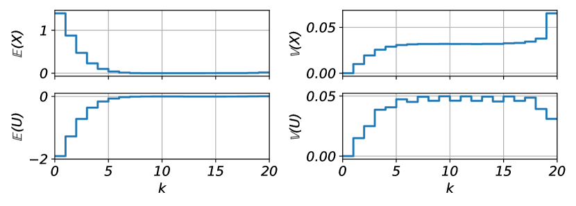
(a) Mean and variance obtained via PCE coefficients.

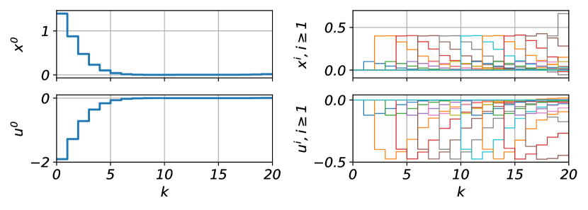
(b) PCE coefficient trajectories.

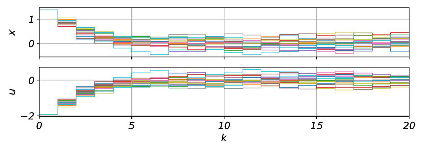
(c) $20$ different realizations trajectories.

Figure 6: Results for the scalar example.

8.2 Descriptor Example

We consider a stochastic extension of the fourth-order linear descriptor system considered in Schmitz et al. [2022b]. The system matrices read

$$E=\begin{bmatrix}0&0&1&0\\ 1&2&0&2\\ 2&3&1&3\\ 1&2&0&2\end{bmatrix},~{}A=\begin{bmatrix}\phantom{-}1&1&0&2\\ \phantom{-}0&2&1&1\\ \phantom{-}1&4&2&3\\ -1&1&1&0\end{bmatrix},~{}B=\begin{bmatrix}-1\\ \phantom{-}2\\ \phantom{-}2\\ \phantom{-}3\end{bmatrix},~{}F=\begin{bmatrix}1\\ 2\\ 3\\ 2\end{bmatrix},$$

$$C=\begin{bmatrix}1&2&1&2\\ 0&1&0&1\end{bmatrix},~{}D=H=0_{2\times 1}.$$

The system can be transformed into quasi-Weierstraß form with $n_{J}=\delta=2$ via the matrices

$$P=\begin{bmatrix}\phantom{-}0&-1&\phantom{-}0&\phantom{-}1\\ -1&\phantom{-}0&\phantom{-}1&\phantom{-}1\\ \phantom{-}1&\phantom{-}0&\phantom{-}0&-1\\ \phantom{-}1&\phantom{-}1&-1&-1\end{bmatrix},~{}S=\begin{bmatrix}\phantom{-}0&-1&\phantom{-}1&\phantom{-}0\\ \phantom{-}1&\phantom{-}2&-1&\phantom{-}0\\ -1&-1&\phantom{-}1&0\\ \phantom{-}0&\phantom{-}1&\phantom{-}0&-1\end{bmatrix}.$$

R-controllability and R-observability are easily verified via Remark 24. Note that in this example we have $F_{N}=0$, which is a special case of $NF_{N}=0$ and hence tightens the causality condition of the input. Thus, causality with respect to the disturbance $W$ is easily obtained in the PCE problem formulation as sketched in Remark 38. For all $k\in\mathds{I}_{[0,N-1]}$, the disturbance $W_{k}$ is modelled as i.i.d. Gaussian random variables with distribution $\mathcal{N}(0,0.1^{2})$.

We want to steer the system to the point $(y,u)=([20,0]^{\top},0)$ and solve the OCP in form of (30) with horizon $N=20$. The weighting matrices in the objective function are chosen to be $Q=I_{2}$ and $R=1$.

In the data collection phase, we record $160$ output-input-noise measurements to construct the Hankel matrices. With respect to the initial condition, we assume no noise measurement is available at run-time. Thus, we model the noise in OCP (30) via its PCE. Moreover, the input applied to the system is randomly sampled from a uniform distribution with support $[-1,1]$. In sum, we obtain the uncertain initial condition (30c) which is modelled via PCE.

Slack variables are added to the initial condition as (31), while we penalize them via the $1$-norm with a weighting parameter. Moreover, since the PCE coefficient of $W$ is known, we employ the null-space method to reduce the dimension of $\mathsf{g}^{i}$ and thus accelerate the computation. For further details we refer to Pan et al. [2022b].

The trajectories of first two moments of $Y$ and $U$ are depicted in Figure 7a while the trajectories of $Y$ and $U$ for $20$ different noise realizations are shown in Figure 7b. Note that in the figure we plot the solution on the horizon length $N=20$ and leave out the additional time steps of the initial condition. Furthermore, we sample a total of 1000 initial conditions as well as the noise realization sequences and compute the corresponding output/input trajectories. The evolution of the normalized histograms of output realizations $y_{1}$ at $k=0,4,9,14,19$ is illustrated in Figure 7c. As one can see, the proposed data-driven optimal control achieves a narrow distribution of $Y_{1}$ around $y_{1}=20$.

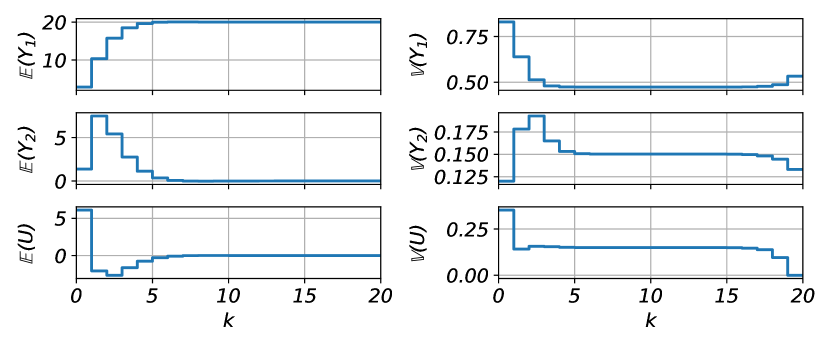
(a) Mean and variance obtained via PCE coefficients.

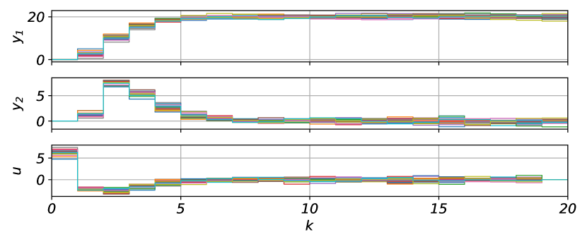
(b) $20$ different realizations trajectories.

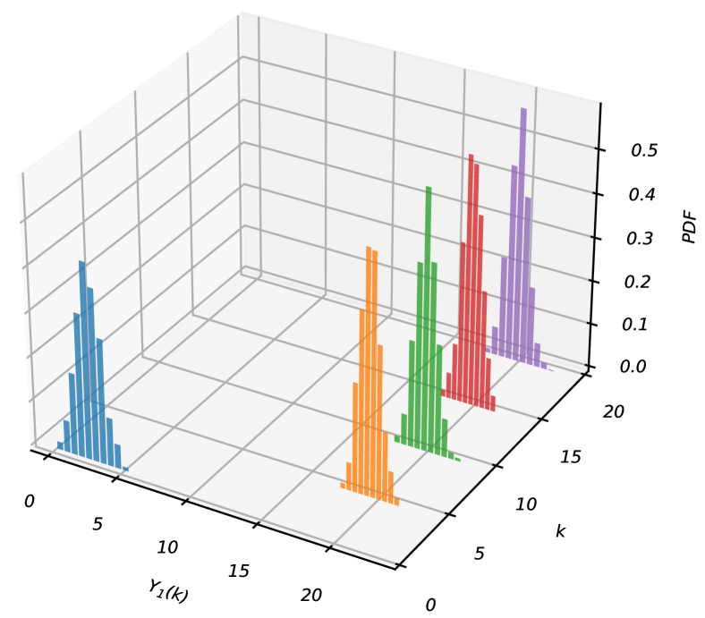
(c) Histograms of the output $Y_{1}$ from $1000$ sampled trajectories.

Figure 7: Results for the descriptor example.

9 Discussion and Open Problems

As discussed in Section 2 the fundamental lemma as such has deep roots in behavioral systems theory. In this tutorial-style paper we proposed extensions of the fundamental lemma to stochastic settings. To this end, we formalized concepts for behavioral characterizations of stochastic systems. We introduced the stochastic $L^{2}$-behavior and its counterpart in terms of series expansion coefficients (which for suitable polynomial chaos expansions can be shown to be finite dimensional). We have analyzed how these behaviors relate to the behavior of sampled trajectories (i.e. the realization behavior). We have also shown that the description in stochastic moments is structurally limited: (i) moments are by their very construction nonlinear projections of random variables, and (ii) this projection, especially if limited to the first two moments, is subject to a substantial loss of information.

Moreover, we remark that the stochastic behavioral description as such does not necessitate the existence of a finite series expansion. Yet, finite-dimensional parametrization of the random-variables fosters numerical tractability in applications.

Coarse $\sigma$-Algebras underlying Stochastic Behaviors. The careful reader has surely recognized that going for PCE as a specific and numerically favourable series expansion of $L^{2}$-random variables is subject to a subtle loss of information in the underlying $\sigma$-algebra, which may potentially jeopardize the equivalence in description established by the lift between the expansion coefficient behavior $\mathfrak{C}_{\infty}$ and the random variable behavior $\mathfrak{S}_{\infty}$, cf. Remark 11. However, as pointed out by Willems [2013] and Baggio & Sepulchre [2017], from a behavioral point of view—and actually also from a dynamical-systems perspective—it is advisable to consider coarse $\sigma$-algebras instead of finer ones. Besides the structure discussed by Willems [2013], Baggio & Sepulchre [2017], where the coarse $\sigma$-algebra is given along the directions perpendicular to the underlying (deterministic) behavior, the loss of information in the context of PCE seems to result in coarseness of a different nature. Hence, two issues arise:

1. To which extent is the information loss in the $\sigma$-algebras induced by the orthogonal PCE basis of major concern?

2. How is this loss related to the coarse algebras suggested by Willems [2013] and Baggio & Sepulchre [2017]?

Indeed, from an engineering perspective, issue (i) appears very much non-critical. Moreover, one may argue that considering the $\sigma$-algebra $\sigma(\mathfrak{F})$, i.e. the one induced by a family $\mathfrak{F}$ of random variables in the context of PCE (cf. Subsection 3.2), instead of the full $\sigma$-algebra $\mathcal{F}$ is a straightforward way of coarsening. Hence, considering $\sigma(\mathfrak{F})$ as the $\sigma$-algebra underlying the considered $L^{2}$-probability space ensures behavioral equivalence. Yet, there may exist other tractable approaches to construct coarse(r) $\sigma$-algebras. Thus issue (ii) calls for further investigations.

Data-driven Output Feedback Predictive Control. While the fundamental lemma has already been published in 2005  [Willems et al., 2005], its impact and reception peaked upon realizing that is opens a path towards data-driven output-feedback predictive control [Yang & Li, 2015, Coulson et al., 2019a] and towards direct data-driven control. Not only does the data-driven approach alleviate the need for explicit identification of a state-space model—it also works with input-output data. Recall that (as per the leading M) MPC as such is traditionally a model-based state-feedback strategy, i.e., observer design is an inevitable step in almost all implementations. The data-driven approach allows to overcome this burden.

In view of the contributions of this tutorial-style paper our developments pave the road towards data-driven output-feedback stochastic predictive control. First steps towards data-driven stochastic MPC, i.e., problem formulation and stability analysis for the case of usual LTI systems with state feedback, have been done by Pan et al. [2022b, d]. At the time of writing these lines, first result on the analysis for the output-feedback case with terminal constraints are available as preprints [Pan et al., 2022a, c]. The extension to the stochastic descriptor case and to closed-loop guarantees without terminal ingredients is completely open.

Another dimension, which will be key for the success of data-driven MPC, are tailored numerical methods. While for model-based MPC powerful codes enable computation times down to a few micro-seconds (depending on the problem size and the computational platform), the results on multiple-shooting formulations of the OCP [Ou et al., 2023]—which we commented on in Section 6—are first steps in this direction. Yet, they leave substantial room for further refinements and improvements.

Robustness. Robustness analysis for data-driven description of deterministic systems has been subject to widespread research efforts, see [Coulson et al., 2019b, Yin et al., 2023, Berberich et al., 2022b, Huang et al., 2023] and the overview [Markovsky & Dörfler, 2021]. We expect that due to the close relation between the realization behavior and the coefficient behavior, cf. Theorem 13, these results can be transferred to the stochastic setting.

Data-driven Analysis of Descriptor Systems. The data-driven approach can be used beyond feedback design. Indeed it also allows analysis of system properties, see, e.g., [Romer et al., 2019b, a] for passivity and dissipativity. When it comes to descriptor systems much less has been done. Specifically, the verification of structural properties besides the dimension of $z^{J}$ in Lemma 31 (nilpotency index, regularity of the matrix pencil, etc.) would be appealing.

Nonlinear Systems. Data-driven control of nonlinear systems is a topic, which has seen substantial progress. One can mention the recent work on data-driven prediction of so-called observables, i.e., real- or complex-valued functions of the state, in the Koopman framework by means of (extended) Dynamic Mode Decomposition (DMD), see [Brunton & Kutz, 2022] as well as the recent surveys by Bevanda et al. [2021] and Brunton et al. [2022] as well as the references therein, or SINDy  [Brunton et al., 2016]. The Koopman framework can also be applied for control. To this end, Proctor et al. [2016] augmented the state dimension $n_{x}$ by the number of input variables $n_{u}$ to set up a surrogate model, see, e.g., [Arbabi et al., 2018, Korda & Mezić, 2018, Mauroy et al., 2020]. To alleviate the curse of dimensionality, Williams et al. [2016], Surana [2016], Klus et al. [2020] proposed a bilinear approach for control-affine systems which shows a superior performance for systems with coupling between state and control, see also [Mauroy et al., 2020, Section 4]. Moreover, Schaller et al. [2023] provide rigorous bounds on the prediction error for control explicitly depending on the dictionary size (projection) and the number of employed data points (estimation). The analysis of the estimation error can be extended to the setting based on stochastic differential equations and ergodic sampling, see [Nüske et al., 2023]. However, data-driven control and fundamental-lemma-type results for nonlinear stochastic systems are not known yet. Similarly, there is substantial prospect of deriving fundamental-lemma-like results for infinite dimensional systems.

10 Conclusions

This paper has taken a fresh look at behavioral theory for stochastic systems. We have constructed equivalent behavioral characterizations of stochastic linear time-invariant systems in terms of $L^{2}$-random variables and in terms of series expansions of these variables. In other words, we have connected the seminal contributions of Jan C. Willems and co-workers with classic concepts put forward by Norbert Wiener.

Importantly, our developments show that there is a synergy of linearity of system structures and the linearity of series expansions of random variables, and of polynomial chaos expansions in particular. This synergy enabled the introduction of novel concepts such as behavioral lifts between different behavioral representations of stochastic systems. The series expansion approach allows to extend the celebrated fundamental lemma to stochastic systems in explicit form and in descriptor form. Crucially, these extensions are built on Hankel matrices comprising realizations of stochastic variables, i.e., they rely on measurement data only.

Thus, the presented contributions open up new perspectives on data-driven control of stochastic systems, on data-driven uncertainty quantification, and on data-driven uncertainty propagation without being restricted to the Gaussian setting.

Appendix

Explicit Reformulation of Descriptor Systems. It is known that descriptor systems allow an equivalent representation in terms of explicit LTI systems—at least in the sense of their manifest behaviors, cf. [Willems, 1986a, Theorem 3] and [Willems, 1991, Section IX.]. However, attaining an explicit LTI representation comes at the expense of inevitable reinterpretation (permutation) of input and output signals which may be unfavorable if chosen inputs and outputs have physical interpretations reflecting on the technical possibilities to measure and to actuate.

Given a manifest behavior $\mathfrak{B}_{\infty}^{\text{i/o}}$ realized by a regular descriptor system (32) we show in the following that there exists a realization $\mathfrak{B}_{\infty}^{\text{i/o}}$ in terms of an explicit LTI system up to some permutation of the input and output variables. Since we consider the manifest behavior, we assume without loss of generality that the descriptor system is in quasi-Weierstraß from (33). We have $(u,y)\in\mathfrak{B}_{\infty}^{\text{i/o}}$ if and only if there is $x^{J}:\mathds{N}\rightarrow\mathds{R}^{n_{J}}$ such that

$$x_{k+1}^{J} =Jx_{k}^{J}+B_{J}u_{k}$$ (56a)

$$y_{k} =C_{J}x^{J}_{k}+Du_{k}-\sum_{i=0}^{\delta-1}C_{N}N^{i}B_{N}u_{k+i}$$ (56b)

for all $k\in\mathds{N}$, cf. (34b) and (36). Observe that it may happen because of the output matrix that $C_{N}N^{\delta-1}B_{N}=0$. Thus deviating from the definition of the structured nilpotency index here we take $\delta$ as the smallest positive integer such that $C_{N}N^{\delta-1}B_{N}\neq 0$ and $C_{N}N^{\delta}B_{N}=0$, or when $C_{N}B_{N}=0$ we set $\delta=1$. In the case $\delta=1$ one sees that (56) is already an explicit LTI system.

Suppose that $\delta>1$ and let $r\doteq\operatorname{rk}(C_{N}N^{\delta-1}B_{N})\geq 1$. We find permutation matrices $T\in\mathds{R}^{n_{y}\times n_{y}}$, $S\in\mathds{R}^{n_{u}\times n_{u}}$ such that for

$$T(D-C_{N}B_{N})S=\begin{bmatrix}\Phi_{0}&\Gamma_{0}\\ F_{0}&G_{0}\end{bmatrix},\quad-TC_{N}N^{i}B_{N}S=\begin{bmatrix}\Phi_{i}&\Gamma_{i}\\ F_{i}&G_{i}\end{bmatrix},$$ (57)

with $\Phi_{0},\Phi_{i}\in\mathds{R}^{r\times r}$ and $i=1,\dots,\delta-1$, the matrix $\Phi_{\delta-1}$ is invertible. As $\operatorname{rk}(C_{N}N^{\delta-1}B_{N})=\operatorname{rk}(\Phi_{\delta-1})=r$ the Schur complement of $-TC_{N}N^{\delta-1}B_{N}S$ with respect to $\Phi_{\delta-1}$ satisfies

$$G_{\delta-1}-F_{\delta-1}\Phi_{\delta-1}^{-1}\Gamma_{\delta-1}=0.$$ (58)

Let $T^{\top}=\begin{bmatrix}T_{1}^{\top}&T_{2}^{\top}\end{bmatrix}$ and $S=\begin{bmatrix}S_{1}&S_{2}\end{bmatrix}$ with $T_{1}\in\mathds{R}^{r\times n_{y}}$, $S_{1}\in\mathds{R}^{n_{u}\times r}$ and decompose the (permuted) input and output signals accordingly,

$$u_{k}=SS^{-1}u_{k}=\begin{bmatrix}S_{1}&S_{2}\end{bmatrix}\begin{bmatrix}\vartheta_{k}\\ \hat{u}_{k}\end{bmatrix},\quad\begin{bmatrix}\eta_{k}\\ \hat{y}_{k}\end{bmatrix}=\begin{bmatrix}T_{1}\\ T_{2}\end{bmatrix}y_{k}=Ty_{k}.$$

Then (56b) is equivalent to

$$\eta_{k} =T_{1}C_{J}x_{k}^{J}-\sum_{i=0}^{\delta-1}\bigl{(}\Phi_{i}\vartheta_{k+i}+\Gamma_{i}\hat{u}_{k+i}\bigr{)}$$ (59a)

$$\hat{y}_{k} =T_{2}C_{J}x_{k}^{J}-\sum_{i=0}^{\delta-1}\bigl{(}F_{i}\vartheta_{k+i}+G_{i}\hat{u}_{k+i}\bigr{)}$$ (59b)

Solving equation (59a) for $\vartheta_{k+\delta-1}$ and plugging this into (59b) one obtains together with (58)

$$\vartheta_{k+\delta-1}={} \Phi_{\delta-1}^{-1}\left(\eta_{k}-T_{1}C_{J}x_{k}^{J}-\sum_{i=0}^{\delta-2}\Phi_{i}\vartheta_{k+i}-\sum_{i=0}^{\delta-1}\Gamma_{i}\hat{u}_{k+i}\right)$$ (60a)

$$\begin{split}\hat{y}_{k}={}&(T_{2}-F_{\delta-1}\Phi_{\delta-1}^{-1}T_{1})C_{J}x_{k}^{J}+F_{\delta-1}\Phi_{\delta-1}^{-1}\eta_{k}\\ &-\sum_{i=0}^{\delta-2}(F_{i}-F_{\delta-1}\Phi_{\delta-1}^{-1}\Phi_{i})\vartheta_{k+i}\\ &-\sum_{i=0}^{\delta-2}(G_{i}-F_{\delta-1}\Phi_{\delta-1}^{-1}\Gamma_{i})\hat{u}_{k+i}\end{split}$$ (60b)

We introduce the augmented state variable

$$\tilde{x}_{k}=\begin{bmatrix}x_{k}^{J}\\ \vartheta_{k}\\ \vdots\\ \vartheta_{k+\delta-2}\end{bmatrix}$$

and the matrix

$$\mathcal{A}=\begin{bmatrix}J&B_{J}S_{1}&0\\ 0&0&I_{r(\delta-2)}\\ -\Phi_{\delta-1}^{-1}T_{1}C_{J}&\Phi_{\delta-1}^{-1}\Phi_{0}&\Phi\end{bmatrix}$$ (61)

with $\Phi=\begin{bmatrix}\Phi_{\delta-1}^{-1}\Phi_{1}&\dots&\Phi_{\delta-1}^{-1}\Phi_{\delta-2}\end{bmatrix}$. The idea of augmentation is borrowed from the continuous-time setting [Ilchmann et al., 2018, 2019], where the state is augmented by derivatives of the control input. Further, let

$$B=\begin{bmatrix}0\\ 0\\ \Phi_{\delta-1}^{-1}\end{bmatrix},\quad\widetilde{B}_{i}=\begin{bmatrix}0\\ 0\\ -\Phi_{\delta-1}^{-1}\Gamma_{i}\end{bmatrix},$$ (62)

$$\mathcal{C}=\begin{bmatrix}0&I_{r}&0\\ (T_{2}-F_{\delta-1}\Phi_{\delta-1}^{-1}T_{1})C_{J}&\Psi_{0}&\Psi\end{bmatrix}$$ (63)

with $\Psi=\begin{bmatrix}\Psi_{1}&\dots&\Psi_{\delta-2}\end{bmatrix}$, where $\Psi_{i}=-(F_{i}-F_{\delta-1}\Phi_{\delta-1}^{-1}\Phi_{i})$. The equations in (60) can be reformulated as

$$\tilde{x}_{k+1} =\mathcal{A}\tilde{x}_{k}+B\eta_{k}+\sum_{i=0}^{\delta-1}\tilde{B}_{i}\hat{u}_{k+i}$$ (64a)

$$\vartheta_{k} =\begin{bmatrix}0&I_{r}&0\end{bmatrix}\tilde{x}_{k}$$ (64b)

$$\hat{y}_{k} =\mathcal{C}\tilde{x}_{k}+F_{\delta-1}\Phi_{\delta-1}^{-1}\eta_{k}-\sum_{i=0}^{\delta-2}(G_{i}-F_{\delta-1}\Phi_{\delta-1}^{-1}\Gamma_{i})\hat{u}_{k+i}.$$ (64c)

We adjust the augmented state variable in order to eliminate of the non-causality in (64a),

$$\hat{x}_{k}\doteq\tilde{x}_{k}-\sum_{i=1}^{\delta-1}\sum_{j=1}^{i}\mathcal{A}^{j-1}\widetilde{B}_{i}\hat{u}_{k+i-j}=\tilde{x}_{k}-\sum_{\gamma=0}^{\delta-2}\sum_{i=\gamma+1}^{\delta-1}\mathcal{A}^{i-\gamma-1}\widetilde{B}_{i}\hat{u}_{k+\gamma},$$ (65)

where the second equality results from a reordering of the summands. We obtain

$$\begin{split}&\tilde{x}_{k+1}-\hat{x}_{k+1}=\sum_{i=1}^{\delta-1}\sum_{j=1}^{i}\mathcal{A}^{j-1}\widetilde{B}_{i}\hat{u}_{k+i-j+1}\\ &=\sum_{i=1}^{\delta-1}\sum_{j=2}^{i}\mathcal{A}^{j-1}\widetilde{B}_{i}\hat{u}_{k+i-j+1}+\sum_{i=1}^{\delta-1}\widetilde{B}_{i}\hat{u}_{k+i}\\ &=\mathcal{A}\sum_{i=1}^{\delta-1}\sum_{j=1}^{i-1}\mathcal{A}^{j-1}\widetilde{B}_{i}\hat{u}_{k+i-j}+\sum_{i=1}^{\delta-1}\widetilde{B}_{i}\hat{u}_{k+i}\\ &=\mathcal{A}\sum_{i=1}^{\delta-1}\sum_{j=1}^{i}\mathcal{A}^{j-1}\widetilde{B}_{i}\hat{u}_{k+i-j}+\sum_{i=1}^{\delta-1}\widetilde{B}_{i}\hat{u}_{k+i}-\sum_{i=1}^{\delta-1}\mathcal{A}^{i}\widetilde{B}_{i}\hat{u}_{k}.\end{split}$$ (66)

Together with (64a) this shows

$$\hat{x}_{k+1}=\mathcal{A}\hat{x}_{k}+B\eta_{k}+\sum_{i=0}^{\delta-1}\mathcal{A}^{i}\widetilde{B}_{i}\hat{u}_{k}$$ (67)

Further, ones sees from (64b) that

$$\vartheta_{k}=\begin{bmatrix}0&I_{r}&0\end{bmatrix}\tilde{x}_{k}=\begin{bmatrix}0&I_{r}&0\end{bmatrix}\left(\hat{x}_{k}+\sum_{i=1}^{\delta-1}\sum_{j=1}^{i}\mathcal{A}^{j-1}\widetilde{B}_{i}\hat{u}_{k+i-j}\right).$$

As $\begin{bmatrix}0&I_{r}&0\end{bmatrix}\mathcal{A}^{j-1}\widetilde{B}_{i}=0$ for $j<\delta-1$ and all $i=0,\dots,\delta-1$ this simplifies to

$$\vartheta_{k}=\begin{bmatrix}0&I_{r}&0\end{bmatrix}\left(\hat{x}_{k}+\mathcal{A}^{\delta-2}\widetilde{B}_{\delta-1}\hat{u}_{k}\right)$$ (68)

Consequently, (64), (67) and (68) yield

$$\hat{x}_{k+1} =\mathcal{A}\hat{x}_{k}+\mathcal{B}\begin{bmatrix}\eta_{k}\\ \hat{u}_{k}\end{bmatrix}$$ (69a)

$$\begin{bmatrix}\vartheta_{k}\\ \hat{y}_{k}\end{bmatrix} =\mathcal{C}\hat{x}_{k}+\mathcal{D}\begin{bmatrix}\eta_{k}\\ \hat{u}_{k}\end{bmatrix}+\sum_{i=1}^{\delta-2}\begin{bmatrix}0&0\\ 0&\Lambda_{i}\end{bmatrix}\begin{bmatrix}\eta_{k+i}\\ \hat{u}_{k+i}\end{bmatrix}$$ (69b)

with $\mathcal{A}$ and $\mathcal{C}$ as in (Appendix) and (63), respectively and

$$\mathcal{B}=\begin{bmatrix}B&\sum_{i=0}^{\delta-1}\mathcal{A}^{i}\widetilde{B}_{i}\end{bmatrix},\quad\mathcal{D}=\begin{bmatrix}0&\mathcal{A}^{\delta-2}\widetilde{B}_{\delta-1}\\ F_{\delta-1}\Phi_{\delta-1}^{-1}&\Lambda_{0}\end{bmatrix},$$

$$\Lambda_{i}=-(G_{i}-F_{\delta-1}\Phi_{\delta-1}^{-1}\Gamma_{i})+\mathcal{C}\sum_{\gamma=i+1}^{\delta-1}A^{\gamma-i-1}\widetilde{B}_{\gamma}.$$

Observe that the manifest variables, that are inputs and outputs jointly together, of (60) are up to some permutation the same as for (69). Moreover, (60) and (69) are structural similar, but in contrast the (60) the highest order of future inputs in (69) is $\delta-2$, and, thus reduces by one order. Although, (69) may still not be in explicit LTI form, further repetitions of the preceding steps, i.e. partially exchanging the role of inputs and outputs variables regarding the rank of $\Lambda_{\delta-2}$ followed by augmentation and adjustment of the state variable, leads to a further decrease in the order. At least after $\delta-2$ additional iterations this results in an explicit LTI realization for $\mathfrak{B}_{\infty}^{\text{i/o}}$ (up to permutation of variables).

References

- AIw [2005] (2005). AI Newsletter. URL: http://www.ainewsletter.com/newsletters/aix_0501.htm#w archived newsletter, accessed 2022-10-10.
- Ahbe et al. [2020] Ahbe, E., Iannelli, A., & Smith, R. S. (2020). Region of attraction analysis of nonlinear stochastic systems using polynomial chaos expansion. Automatica, 122, 109187.
- Alsalti et al. [2021] Alsalti, M., Berberich, V. G., J.and Lopez, Allgöwer, F., & Müller, M. A. (2021). Data-based system analysis and control of flat nonlinear systems. In Proc. 2021 60th IEEE Conference on Decision and Control (pp. 1484–1489). IEEE.
- Arbabi et al. [2018] Arbabi, H., Korda, M., & Mezić, I. (2018). A data-driven Koopman model predictive control framework for nonlinear partial differential equations. In Proc. 2018 57th IEEE Conference on Decision and Control (pp. 6409–6414). IEEE.
- Axehill [2015] Axehill, D. (2015). Controlling the level of sparsity in MPC. Systems & Control Letters, 76, 1–7.
- Baggio & Sepulchre [2017] Baggio, G., & Sepulchre, R. (2017). LTI stochastic processes: A behavioral perspective. IFAC-PapersOnLine, 50(1), 2806–2811.
- Ball & Staffans [2006] Ball, J. A., & Staffans, O. J. (2006). Conservative state-space realizations of dissipative system behaviors. Integral Equations and Operator Theory, 54(2), 151–213.
- Baudin et al. [2017] Baudin, M., Dutfoy, A., Iooss, B., & Popelin, A.-L. (2017). OpenTURNS: An industrial software for uncertainty quantification in simulation. In Handbook of Uncertainty Quantification (pp. 2001–2038). Cham: Springer International Publishing.
- Belov et al. [2018] Belov, A. A., Andrianova, O. G., & Kurdyukov, A. P. (2018). Control of Discrete-Time Descriptor Systems. An Anisotropy-Based Approach volume 157. Cham: Springer. doi:10.1007/978-3-319-78479-3.
- Berberich & Allgöwer [2020] Berberich, J., & Allgöwer, F. (2020). A trajectory-based framework for data-driven system analysis and control. In Proc. 2020 European Control Conference (pp. 1365–1370). IEEE.
- Berberich et al. [2022a] Berberich, J., Köhler, J., Müller, M. A., & Allgöwer, F. (2022a). Linear tracking MPC for nonlinear systems Part II: The data-driven case. IEEE Transactions on Automatic Control, 67(9), 4406–4421. doi:10.1109/tac.2022.3166851.
- Berberich et al. [2022b] Berberich, J., Scherer, C. W., & Allgöwer, F. (2022b). Combining prior knowledge and data for robust controller design. IEEE Transactions on Automatic Control, (pp. 1–16). doi:10.1109/TAC.2022.3209342.
- Berger et al. [2012] Berger, T., Ilchmann, A., & Trenn, S. (2012). The quasi-Weierstrass form for regular matrix pencils. Linear Algebra and its Applications, 436(10), 4052–4069. doi:10.1016/j.laa.2009.12.036.
- Berger & Reis [2013] Berger, T., & Reis, T. (2013). Controllability of linear differential-algebraic systems – A survey. In Surveys in Differential-Algebraic Equations I (pp. 1–61). Berlin: Springer.
- Bevanda et al. [2021] Bevanda, P., Sosnowski, S., & Hirche, S. (2021). Koopman operator dynamical models: Learning, analysis and control. Annual Reviews in Control, 52, 197–212.
- Biegler et al. [2012] Biegler, L. T., Campbell, S. L., & Mehrmann, V. (2012). Control and optimization with differential-algebraic constraints. SIAM.
- Bienstock et al. [2014] Bienstock, D., Chertkov, M., & Harnett, S. (2014). Chance-constrained optimal power flow: Risk-aware network control under uncertainty. SIAM Review, 56(3), 461–495. doi:10.1137/130910312.
- Bilgic et al. [2022] Bilgic, D., Koch, A., Pan, G., & Faulwasser, T. (2022). Toward data-driven predictive control of multi-energy distribution systems. Electric Power Systems Research, 212, 108311. doi:https://doi.org/10.1016/j.epsr.2022.108311.
- Bock & Plitt [1984] Bock, H. G., & Plitt, K.-J. (1984). A multiple shooting algorithm for direct solution of optimal control problems. IFAC Proceedings Volumes, 17(2), 1603–1608.
- Brezis [2011] Brezis, H. (2011). Functional Analysis, Sobolev Spaces and Partial Differential Equations volume 2. Springer.
- Brunton et al. [2022] Brunton, S. L., Budišić, M., Kaiser, E., & Kutz, J. N. (2022). Modern Koopman theory for dynamical systems. SIAM Review, 64(2), 229–340. doi:10.1137/21M1401243.
- Brunton & Kutz [2022] Brunton, S. L., & Kutz, J. N. (2022). Data-driven science and engineering: Machine learning, dynamical systems, and control. Cambridge University Press.
- Brunton et al. [2016] Brunton, S. L., Proctor, J. L., & Kutz, J. N. (2016). Discovering governing equations from data by sparse identification of nonlinear dynamical systems. Proceedings of the National Academy of Sciences, 113(15), 3932–3937.
- Calafiore & Ghaoui [2006] Calafiore, G. C., & Ghaoui, L. E. (2006). On distributionally robust chance-constrained linear programs. Journal of Optimization Theory and Applications, 130(1), 1–22.
- Cameron & Martin [1947] Cameron, R. H., & Martin, W. T. (1947). The orthogonal development of non-linear functionals in series of fourier-hermite functionals. Annals of Mathematics, (pp. 385–392).
- Campbell et al. [2019] Campbell, S., Ilchmann, A., Mehrmann, V., Reis, T. et al. (2019). Applications of differential-algebraic equations: examples and benchmarks. Springer.
- Campi & Garatti [2018] Campi, M. C., & Garatti, S. (2018). Introduction to the Scenario Approach. SIAM. doi:10.1137/1.9781611975444.
- Campi et al. [2009] Campi, M. C., Garatti, S., & Prandini, M. (2009). The scenario approach for systems and control design. Annual Reviews in Control, 33(2), 149–157.
- Carlet et al. [2020] Carlet, P. G., Favato, A., Bolognani, S., & Dörfler, F. (2020). Data-driven predictive current control for synchronous motor drives. In Proc. 2020 IEEE Energy Conversion Congress and Exposition (ECCE) (pp. 5148–5154). IEEE.
- Coulson et al. [2019a] Coulson, J., Lygeros, J., & Dörfler, F. (2019a). Data-enabled predictive control: In the shallows of the DeePC. In Proc. 2019 European Control Conference (pp. 307–312). IEEE.
- Coulson et al. [2019b] Coulson, J., Lygeros, J., & Dörfler, F. (2019b). Regularized and distributionally robust data-enabled predictive control. In Proc. 2019 58th IEEE Conference on Decision and Control (pp. 2696–2701). IEEE.
- Cremer et al. [2018] Cremer, J. L., Konstantelos, I., Tindemans, S. H., & Strbac, G. (2018). Data-driven power system operation: Exploring the balance between cost and risk. IEEE Transactions on Power Systems, 34(1), 791–801.
- Dai [1989] Dai, L. (1989). Singular Control Systems volume 118. Berlin etc.: Springer-Verlag.
- De Persis & Tesi [2019] De Persis, C., & Tesi, P. (2019). Formulas for data-driven control: Stabilization, optimality, and robustness. IEEE Transactions on Automatic Control, 65(3), 909–924.
- Deisenroth et al. [2013] Deisenroth, M. P., Fox, D., & Rasmussen, C. E. (2013). Gaussian processes for data-efficient learning in robotics and control. IEEE Transactions on Pattern Analysis and Machine Intelligence, 37(2), 408–423.
- Dörfler et al. [2022] Dörfler, F., Coulson, J., & Markovsky, I. (2022). Bridging direct & indirect data-driven control formulations via regularizations and relaxations. IEEE Transactions on Automatic Control, (pp. 1–1). doi:10.1109/TAC.2022.3148374.
- Dörfler et al. [2021] Dörfler, F., Tesi, P., & De Persis, C. (2021). On the certainty-equivalence approach to direct data-driven LQR design. ArXiv preprint arXiv:2109.06643.
- Ernst et al. [2012] Ernst, O. G., Mugler, A., Starkloff, H.-J., & Ullmann, E. (2012). On the convergence of generalized polynomial chaos expansions. ESAIM: Mathematical Modelling and Numerical Analysis, 46(2), 317–339.
- Fagiano & Khammash [2012] Fagiano, L., & Khammash, M. (2012). Nonlinear stochastic model predictive control via regularized polynomial chaos expansions. In Proc. 2012 51st IEEE conference on decision and control (pp. 142–147). IEEE.
- Farina et al. [2016] Farina, M., Giulioni, L., & Scattolini, R. (2016). Stochastic linear model predictive control with chance constraints–A review. Journal of Process Control, 44, 53–67.
- Faulwasser & Grüne [2022] Faulwasser, T., & Grüne, L. (2022). Turnpike properties in optimal control: An overview of discrete-time and continuous-time results. In E. Zuazua, & E. Trelat (Eds.), Handbook of Numerical Analysis chapter 11. (pp. 367–400). Elsevier volume 23. doi:10.1016/bs.hna.2021.12.011 arxiv: 2011.13670.
- Favoreel et al. [1999] Favoreel, W., De Moor, B., & Gevers, M. (1999). SPC: Subspace predictive control. IFAC Proceedings Volumes, 32(2), 4004–4009.
- Feinberg & Langtangen [2015] Feinberg, J., & Langtangen, H. P. (2015). Chaospy: An open source tool for designing methods of uncertainty quantification. Journal of Computational Science, 11, 46–57.
- Fiedler & Lucia [2021] Fiedler, F., & Lucia, S. (2021). On the relationship between data-enabled predictive control and subspace predictive control. In Proc. 2021 European Control Conference (pp. 222–229). IEEE.
- Field & Grigoriu [2004] Field, R. V., & Grigoriu, M. (2004). On the accuracy of the polynomial chaos approximation. Probabilistic Engineering Mechanics, 19(1), 65–80. doi:https://doi.org/10.1016/j.probengmech.2003.11.017.
- Fisher & Bhattacharya [2008] Fisher, J., & Bhattacharya, R. (2008). On stochastic LQR design and polynomial chaos. In Proc. 2008 American Control Conference (ACC) (pp. 95–100). IEEE.
- Ghanem & Spanos [2003] Ghanem, R. G., & Spanos, P. D. (2003). Stochastic Finite Elements: A Spectral Approach. (Revised ed.). Springer New York.
- Givens & Shortt [1984] Givens, C. R., & Shortt, R. M. (1984). A class of Wasserstein metrics for probability distributions. Michigan Mathematical Journal, 31(2), 231–240.
- Groß et al. [2016] Groß, T., Trenn, S., & Wirsen, A. (2016). Solvability and stability of a power system dae model. Systems & Control Letters, 97, 12–17.
- Heirung et al. [2018] Heirung, T. A. N., Paulson, J. A., O’Leary, J., & Mesbah, A. (2018). Stochastic model predictive control—how does it work? Computers & Chemical Engineering, 114, 158–170.
- Huang et al. [2019] Huang, L., Coulson, J., Lygeros, J., & Dörfler, F. (2019). Data-enabled predictive control for grid-connected power converters. In Proc. 2019 58th IEEE Conference on Decision and Control (pp. 8130–8135). IEEE.
- Huang et al. [2021] Huang, L., Coulson, J., Lygeros, J., & Dörfler, F. (2021). Decentralized data-enabled predictive control for power system oscillation damping. IEEE Transactions on Control Systems Technology, 30(3), 1065–1077.
- Huang et al. [2022] Huang, L., Lygeros, J., & Dörfler, F. (2022). Robust and kernelized data-enabled predictive control for nonlinear systems. ArXiv preprint arXiv:2206.01866.
- Huang et al. [2023] Huang, L., Zhen, J., Lygeros, J., & Dörfler, F. (2023). Robust data-enabled predictive control: Tractable formulations and performance guarantees. IEEE Transactions on Automatic Control, .
- Hüllermeier & Waegeman [2021] Hüllermeier, E., & Waegeman, W. (2021). Aleatoric and epistemic uncertainty in machine learning: An introduction to concepts and methods. Machine Learning, 110(3), 457–506.
- Ilchmann et al. [2019] Ilchmann, A., Leben, L., Witschel, J., & Worthmann, K. (2019). Optimal control of differential-algebraic equations from an ordinary differential equation perspective. Optimal Control Applications and Methods, 40(2), 351–366.
- Ilchmann et al. [2018] Ilchmann, A., Witschel, J., & Worthmann, K. (2018). Model predictive control for linear differential-algebraic equations. IFAC-PapersOnLine, 51(20), 98–103.
- Katayama [2006] Katayama, T. (2006). A system theoretic interpretation of LQ decomposition in subspace identification methods. In Proc. 2006 17th Int. Symposium on Mathematical Theory of Networks and Systems (MTNS). Kyoto, Japan (pp. 1089–1095).
- Kerz et al. [2021] Kerz, S., Teutsch, J., Brüdigam, T., Wollherr, D., & Leibold, M. (2021). Data-driven stochastic model predictive control. ArXiv preprint arXiv:2112.04439.
- Kim et al. [2013] Kim, K.-K. K., Shen, D. E., Nagy, Z. K., & Braatz, R. D. (2013). Wiener’s polynomial chaos for the analysis and control of nonlinear dynamical systems with probabilistic uncertainties [historical perspectives]. IEEE Control Systems Magazine, 33(5), 58–67.
- Klenke [2013] Klenke, A. (2013). Probability Theory: A Comprehensive Course. Springer Science & Business Media.
- Klus et al. [2020] Klus, S., Nüske, F., Peitz, S., Niemann, J.-H., Clementi, C., & Schütte, C. (2020). Data-driven approximation of the Koopman generator: Model reduction, system identification, and control. Physica D: Nonlinear Phenomena, 406, 132416.
- Koekoek & Swarttouw [1998] Koekoek, R., & Swarttouw, R. F. (1998). The Askey-scheme of hypergeometric orthogonal polynomials and its q-analogue. Technical Report 98-17 Department of Technical Mathematics and Informatics, Delft University of Technology Delft, The Netherlands.
- Korda & Mezić [2018] Korda, M., & Mezić, I. (2018). Linear predictors for nonlinear dynamical systems: Koopman operator meets model predictive control. Automatica, 93, 149–160.
- Kuehn [2016] Kuehn, C. (2016). Moment Closure—A Brief Review. Control of Self-Organizing Nonlinear Systems, (pp. 253–271).
- Kunkel & Mehrmann [2006] Kunkel, P., & Mehrmann, V. (2006). Differential-algebraic equations: Analysis and numerical solution volume 2. European Mathematical Society.
- Lefebvre [2020] Lefebvre, T. (2020). On moment estimation from polynomial chaos expansion models. IEEE Control Systems Letters, 5(5), 1519–1524.
- Lian & Jones [2021] Lian, Y., & Jones, C. N. (2021). Nonlinear data-enabled prediction and control. In Proc. 3rd Conference on Learning for Dynamics and Control (pp. 523–534). PMLR volume 144 of Proceedings of Machine Learning Research.
- Lian et al. [2021] Lian, Y., Shi, J., Koch, M. P., & Jones, C. N. (2021). Adaptive robust data-driven building control via bi-level reformulation: an experimental result. ArXiv preprint arXiv:2106.05740.
- Malliavin et al. [1995] Malliavin, P., Airault, H., Kay, L., & Letac, G. (1995). Integration and Probability volume 157. Springer Science & Business Media.
- Markovsky [2021] Markovsky, I. (2021). Data-driven simulation of nonlinear systems via linear time-invariant embedding. Vrije Universiteit Brussel, . Technical Report.
- Markovsky & Dörfler [2021] Markovsky, I., & Dörfler, F. (2021). Behavioral systems theory in data-driven analysis, signal processing, and control. Annual Reviews in Control, 52, 42–64.
- Markovsky et al. [2006] Markovsky, I., Willems, J. C., Van Huffel, S., & De Moor, B. (2006). Exact and Approximate Modeling of Linear Systems. A Behavioral Approach volume 11 of Math. Model. Comput.. Philadelphia, PA: Society for Industrial and Applied Mathematics (SIAM). doi:10.1137/1.9780898718263.
- Martinelli et al. [2022] Martinelli, A., Gargiani, M., Draskovic, M., & Lygeros, J. (2022). Data-driven optimal control of affine systems: A linear programming perspective. IEEE Control Systems Letters, 6, 3092–3097. doi:10.1109/LCSYS.2022.3180898.
- Mauroy et al. [2020] Mauroy, A., Susuki, Y., & Mezić, I. (2020). Koopman operator in systems and control. Springer.
- Mesbah [2016] Mesbah, A. (2016). Stochastic model predictive control: An overview and perspectives for future research. IEEE Control Systems, 36(6), 30–44.
- Mesbah & Streif [2015] Mesbah, A., & Streif, S. (2015). A probabilistic approach to robust optimal experiment design with chance constraints. IFAC-PapersOnLine, 48(8), 100–105.
- Milano & Zárate-Miñano [2013] Milano, F., & Zárate-Miñano, R. (2013). A systematic method to model power systems as stochastic differential algebraic equations. IEEE Transactions on Power Systems, 28(4), 4537–4544.
- Mohajerin Esfahani & Kuhn [2018] Mohajerin Esfahani, P., & Kuhn, D. (2018). Data-driven distributionally robust optimization using the Wasserstein metric: Performance guarantees and tractable reformulations. Mathematical Programming, 171(1), 115–166.
- Moonen et al. [1989] Moonen, M., De Moor, B., Vandenberghe, L., & Vandewalle, J. (1989). On- and off-line identification of linear state-space models. International Journal of Control, 49(1), 219–232.
- Muandet et al. [2017] Muandet, K., Fukumizu, K., Sriperumbudur, B., Schölkopf, B. et al. (2017). Kernel mean embedding of distributions: A review and beyond. Foundations and Trends® in Machine Learning, 10(1-2), 1–141.
- Mühlpfordt et al. [2018a] Mühlpfordt, T., Faulwasser, T., & Hagenmeyer, V. (2018a). A generalized framework for chance-constrained optimal power flow. Sustainable Energy, Grids and Networks, 16, 231–242. doi:10.1016/j.segan.2018.08.002. ArXiv:1803.08299.
- Mühlpfordt et al. [2017] Mühlpfordt, T., Faulwasser, T., Roald, L., & Hagenmeyer, V. (2017). Solving optimal power flow with non-Gaussian uncertainties via polynomial chaos expansion. In Proc. 2017 56th IEEE Conference on Decision and Control (pp. 4490–4496). doi:10.1109/CDC.2017.8264321.
- Mühlpfordt et al. [2018b] Mühlpfordt, T., Findeisen, R., Hagenmeyer, V., & Faulwasser, T. (2018b). Comments on quantifying truncation errors for polynomial chaos expansions. IEEE Control Systems Letters, 2(1), 169–174. doi:10.1109/LCSYS.2017.2778138.
- Mühlpfordt et al. [2020] Mühlpfordt, T., Zahn, F., Hagenmeyer, V., & Faulwasser, T. (2020). PolyChaos.jl—A julia package for polynomial chaos in systems and control. IFAC-PapersOnLine, 53(2), 7210–7216. doi:10.1016/j.ifacol.2020.12.552. 21th IFAC World Congress.
- Nagy & Braatz [2007] Nagy, Z. K., & Braatz, R. D. (2007). Distributional uncertainty analysis using power series and polynomial chaos expansions. Journal of Process Control, 17(3), 229–240.
- Nortmann & Mylvaganam [2021] Nortmann, B., & Mylvaganam, T. (2021). Direct data-driven control of linear time-varying systems. ArXiv preprint arXiv:2111.02342.
- Nüske et al. [2023] Nüske, F., Peitz, S., Philipp, F., Schaller, M., & Worthmann, K. (2023). Finite-data error bounds for Koopman-based prediction and control. Journal of Nonlinear Science, 33, 14.
- Ou et al. [2021] Ou, R., Baumann, M. H., Grüne, L., & Faulwasser, T. (2021). A simulation study on turnpikes in stochastic LQ optimal control. IFAC-PapersOnLine, 54(3), 516–521. doi:https://doi.org/10.1016/j.ifacol.2021.08.294.
- Ou et al. [2023] Ou, R., Pan, G., & Faulwasser, T. (2023). Data-driven multiple shooting for stochastic optimal control. IEEE Control Systems Letters, 7, 313–318. doi:10.1109/LCSYS.2022.3185841.
- O’Dwyer et al. [2022] O’Dwyer, E., Kerrigan, E. C., Falugi, P., Zagorowska, M., & Shah, N. (2022). Data-driven predictive control with improved performance using segmented trajectories. IEEE Transactions on Control Systems Technology, (pp. 1–11). doi:10.1109/TCST.2022.3224330.
- O’Hagan [2013] O’Hagan, A. (2013). Polynomial chaos: A tutorial and critique from a statistician’s perspective. SIAM/ASA J. Uncertainty Quantification, 20, 1–20.
- Pan et al. [2022a] Pan, G., Ou, R., & Faulwasser, T. (2022a). Data-driven stochastic output-feedback predictive control: Recursive feasibility through interpolated initial conditions. ArXiv preprint arXiv:2212.07661.
- Pan et al. [2022b] Pan, G., Ou, R., & Faulwasser, T. (2022b). On a stochastic fundamental lemma and its use for data-driven optimal control. IEEE Transactions on Automatic Control, (pp. 1–16). doi:10.1109/TAC.2022.3232442.
- Pan et al. [2022c] Pan, G., Ou, R., & Faulwasser, T. (2022c). On data-driven stochastic output-feedback predictive control. ArXiv preprint arXiv:2211.17074.
- Pan et al. [2022d] Pan, G., Ou, R., & Faulwasser, T. (2022d). Towards data-driven stochastic predictive control. ArXiv preprint arXiv:2212.10663.
- Petzke et al. [2020] Petzke, F., Mesbah, A., & Streif, S. (2020). PoCET: a polynomial chaos expansion toolbox for Matlab. IFAC-PapersOnLine, 53(2), 7256–7261.
- Pillai & Shankar [1999] Pillai, H. K., & Shankar, S. (1999). A behavioral approach to control of distributed systems. SIAM Journal on Control and Optimization, 37(2), 388–408.
- Pillai & Willems [1999] Pillai, H. K., & Willems, J. C. (1999). The behavioural approach to distributed systems. In Procc 1999 38th IEEE Conference on Decision and Control (pp. 626–630). IEEE.
- Pillai & Willems [2002] Pillai, H. K., & Willems, J. C. (2002). Lossless and dissipative distributed systems. SIAM Journal on Control and Optimization, 40(5), 1406–1430.
- Pola [2017] Pola, G. (2017). On achievable behavior of stochastic descriptor systems. In Proc. 2017 56th IEEE Conference on Decision and Control (pp. 3164–3169). IEEE.
- Pola et al. [2016] Pola, G., Manes, C., & Di Benedetto, M. D. (2016). On external behavior equivalence of continuous-time stochastic linear control systems. In Proc. 2016 IEEE 55th Conference on Decision and Control (pp. 6583–6588). IEEE.
- Pola et al. [2015] Pola, G., Manes, C., van der Schaft, A. J., & Di Benedetto, M. D. (2015). On equivalence notions for discrete-time stochastic control systems. In Proc. 2015 54th IEEE Conference on Decision and Control (pp. 1180–1185). IEEE.
- Polderman & Willems [1997] Polderman, J. W., & Willems, J. C. (1997). Introduction to Mathematical Systems Theory. A Behavioral Approach volume 26. New York, NY: Springer.
- Proctor et al. [2016] Proctor, J. L., Brunton, S. L., & Kutz, J. N. (2016). Dynamic mode decomposition with control. SIAM J. Applied Dynamical Systems, 15(1), 142–161.
- Rainville [1960] Rainville, E. (1960). Special functions. Macmillan.
- Romer et al. [2019a] Romer, A., Berberich, J., Köhler, J., & Allgöwer, F. (2019a). One-shot verification of dissipativity properties from input–output data. IEEE Control Systems Letters, 3(3), 709–714.
- Romer et al. [2019b] Romer, A., Trimpe, S., & Allgöwer, F. (2019b). Data-driven inference of passivity properties via Gaussian process optimization. In Proc. 2019 European Control Conference (pp. 29–35). IEEE.
- Rueda-Escobedo et al. [2022] Rueda-Escobedo, J. G., Fridman, E., & Schiffer, J. (2022). Data-driven control for linear discrete-time delay systems. IEEE Transactions on Automatic Control, 67(7), 3321–3336. doi:10.1109/TAC.2021.3096896.
- Rueda-Escobedo & Schiffer [2020] Rueda-Escobedo, J. G., & Schiffer, J. (2020). Data-driven internal model control of second-order discrete volterra systems. In Proc. 2020 59th IEEE Conference on Decision and Control (pp. 4572–4579). IEEE.
- Schaller et al. [2023] Schaller, M., Worthmann, K., Philipp, F., Peitz, S., & Nüske, F. (2023). Towards reliable data-based optimal and predictive control using extended DMD. IFAC-PapersOnLine, 56(1), 169–174.
- Schmitz et al. [2022a] Schmitz, P., Engelmann, A., Faulwasser, T., & Worthmann, K. (2022a). Data-driven MPC of descriptor systems: A case study for power networks. IFAC PapersOnLine, 55(30), 359–364.
- Schmitz et al. [2022b] Schmitz, P., Faulwasser, T., & Worthmann, K. (2022b). Willems’ fundamental lemma for linear descriptor systems and its use for data-driven output-feedback MPC. IEEE Control Systems Letters, 6, 2443–2448. doi:10.1109/LCSYS.2022.3161054.
- Seiler & Zerz [2015] Seiler, W. M., & Zerz, E. (2015). Algebraic theory of linear systems: A survey. In Surveys in Differential-Algebraic Equations II (pp. 287–333). Springer.
- Singh & Hespanha [2010] Singh, A., & Hespanha, J. P. (2010). Approximate moment dynamics for chemically reacting systems. IEEE Transactions on Automatic Control, 56(2), 414–418.
- Sontag [1998] Sontag, E. (1998). Mathematical Control Theory: Deterministic Finite Dimensional Systems volume 6. Springer.
- Stykel [2002] Stykel, T. (2002). Analysis and numerical solution of generalized Lyapunov equations. dissertation TU Berlin.
- Sullivan [2015] Sullivan, T. J. (2015). Introduction to Uncertainty Quantification volume 63. Springer.
- Surana [2016] Surana, A. (2016). Koopman operator based observer synthesis for control-affine nonlinear systems. In Proc. 2016 55th IEEE Conference Decision Control (CDC) (pp. 6492–6499).
- Umlauft et al. [2020] Umlauft, J., Lederer, A., Beckers, T., & Hirche, S. (2020). Real-time uncertainty decomposition for online learning control. ArXiv preprint arXiv:2010.02613.
- Venzke et al. [2021] Venzke, A., Molzahn, D. K., & Chatzivasileiadis, S. (2021). Efficient creation of datasets for data-driven power system applications. Electric Power Systems Research, 190, 106614.
- Verhaegen [2015] Verhaegen, M. (2015). Subspace techniques in system identification. In Encyclopedia of Systems and Control (pp. 1386–1396). Springer. doi:10.1007/978-1-4471-5058-9_107.
- Verhoek et al. [2021] Verhoek, C., Tóth, R., Haesaert, S., & Koch, A. (2021). Fundamental lemma for data-driven analysis of linear parameter-varying systems. In Proc. 2021 60th IEEE Conference on Decision and Control (pp. 5040–5046). IEEE.
- van Waarde et al. [2022] van Waarde, H. J., Camlibel, M. K., & Mesbahi, M. (2022). From noisy data to feedback controllers: non-conservative design via a matrix S-lemma. IEEE Transactions on Automatic Control, 67(1), 162–175. doi:10.1109/TAC.2020.3047577.
- van Waarde et al. [2020] van Waarde, H. J., De Persis, C., Camlibel, M. K., & Tesi, P. (2020). Willems’ fundamental lemma for state-space systems and its extension to multiple datasets. IEEE Control Systems Letters, 4(3), 602–607.
- Wan et al. [2023] Wan, Y., Shen, D., Lucia, S., Findeisen, R., & Braatz, R. D. (2023). A polynomial chaos approach to robust H_infinity static output-feedback control with bounded truncation error. IEEE Transactions on Automatic Control, 68(1), 470–477. doi:10.1109/TAC.2022.3140275.
- Wan et al. [2021] Wan, Y., Shen, D. E., Lucia, S., Findeisen, R., & Braatz, R. D. (2021). Polynomial chaos-based H2 output-feedback control of systems with probabilistic parametric uncertainties. Automatica, 131, 109743.
- Wang et al. [2022] Wang, J., Zheng, Y., Li, K., & Xu, Q. (2022). DeeP-LCC: Data-enabled predictive leading cruise control in mixed traffic flow. ArXiv preprint arXiv:2203.10639.
- Wiener [1938] Wiener, N. (1938). The homogeneous chaos. American Journal of Mathematics, (pp. 897–936).
- Willems [1986a] Willems, J. C. (1986a). From time series to linear system—Part I. Finite dimensional linear time invariant systems. Automatica, 22(5), 561–580.
- Willems [1986b] Willems, J. C. (1986b). From time series to linear system—Part II. Exact modelling. Automatica, 22(6), 675–694.
- Willems [1987] Willems, J. C. (1987). From time series to linear system—Part III: Approximate modelling. Automatica, 23(1), 87–115.
- Willems [1991] Willems, J. C. (1991). Paradigms and puzzles in the theory of dynamical systems. IEEE Transactions on Automatic Control, 36(3), 259–294.
- Willems [2007] Willems, J. C. (2007). The behavioral approach to open and interconnected systems. IEEE Control Systems Magazine, 27(6), 46–99.
- Willems [2013] Willems, J. C. (2013). Open stochastic systems. IEEE Transactions on Automatic Control, 58(2), 406–421.
- Willems et al. [2005] Willems, J. C., Rapisarda, P., Markovsky, I., & De Moor, B. L. M. (2005). A note on persistency of excitation. Systems & Control Letters, 54(4), 325–329. doi:10.1016/j.sysconle.2004.09.003.
- Williams et al. [2016] Williams, M. O., Hemati, M. S., Dawson, S. T., Kevrekidis, I. G., & Rowley, C. W. (2016). Extending data-driven Koopman analysis to actuated systems. IFAC-PapersOnLine, 49(18), 704–709.
- Wood & Zerz [1999] Wood, J., & Zerz, E. (1999). Notes on the definition of behavioural controllability. Systems & Control Letters, 37(1), 31–37.
- Xiu [2010] Xiu, D. (2010). Numerical Methods for Stochastic Computations. Princeton University Press.
- Xiu & Karniadakis [2002] Xiu, D., & Karniadakis, G. E. (2002). The Wiener–Askey polynomial chaos for stochastic differential equations. SIAM Journal on Scientific Computing, 24(2), 619–644.
- Yamamoto & Willems [2008] Yamamoto, Y., & Willems, J. C. (2008). Behavioral controllability and coprimeness for a class of infinite-dimensional systems. In Proc. 2008 47th IEEE Conference on Decision and Control (pp. 1513–1518). IEEE.
- Yan et al. [2018] Yan, L., Duan, X., Liu, B., & Xu, J. (2018). Gaussian processes and polynomial chaos expansion for regression problem: linkage via the RKHS and comparison via the KL divergence. Entropy, 20(3), 191.
- Yang & Li [2015] Yang, H., & Li, S. (2015). A data-driven predictive controller design based on reduced Hankel matrix. In 2015 10th Asian Control Conference (ASCC) (pp. 1–7). IEEE.
- Yin et al. [2022] Yin, M., Iannelli, A., & Smith, R. S. (2022). Data-driven prediction with stochastic data: Confidence regions and minimum mean-squared error estimates. In Proc. 2022 European Control Conference (pp. 853–858). doi:10.23919/ECC55457.2022.9838046.
- Yin et al. [2023] Yin, M., Iannelli, A., & Smith, R. S. (2023). Maximum likelihood estimation in data-driven modeling and control. IEEE Transactions on Automatic Control, 68(1), 317–328. doi:10.1109/TAC.2021.3137788.
- Yu et al. [2021] Yu, Y., Talebi, S., van Waarde, H. J., Topcu, U., Mesbahi, M., & Açıkmeșe, B. (2021). On controllability and persistency of excitation in data-driven control: Extensions of Willems’ fundamental lemma. In Proc. 2021 60th IEEE Conference on Decision and Control (pp. 6485–6490). IEEE.
- Yuan & Cortés [2022] Yuan, Z., & Cortés, J. (2022). Data-driven optimal control of bilinear systems. IEEE Control Systems Letters, 6, 2479–2484.
- Zavala [2014] Zavala, V. M. (2014). Stochastic optimal control model for natural gas networks. Computers & Chemical Engineering, 64, 103–113.
- Zhang et al. [2020] Zhang, H., Harlim, J., & Li, X. (2020). Estimating linear response statistics using orthogonal polynomials: An RKHS formulation. Foundations of Data Science, 2(4), 443–485.