Distributed algorithm for continuous-type Bayesian Nash Equilibrium in Subnetwork Zero-sum Games††This work was supported by the National Natural Science Foundation of China (No. 62173250), and by Shanghai Municipal Science and Technology Major Project (No. 2021SHZDZX0100).
Abstract
In this paper, we consider a continuous-type Bayesian Nash equilibrium (BNE) seeking problem in subnetwork zero-sum games, which is a generalization of deterministic subnetwork zero-sum games and discrete-type Bayesian zero-sum games. In this continuous-type model, because the feasible strategy set is composed of infinite-dimensional functions and is not compact, it is hard to seek a BNE in a non-compact set and convey such complex strategies in network communication. To this end, we design two steps to overcome the above bottleneck. One is a discretization step, where we discretize continuous types and prove that the BNE of the discretized model is an approximate BNE of the continuous model with an explicit error bound. The other one is a communication step, where we adopt a novel compression scheme with a designed sparsification rule and prove that agents can obtain unbiased estimations through compressed communication. Based on the above two steps, we propose a distributed communication-efficient algorithm to practicably seek an approximate BNE, and further provide an explicit error bound and an convergence rate.
Keywords: Bayesian game, subnetwork zero-sum game, distributed algorithm, equilibrium approximation, communication compression
1 Introduction
In recent years, distributed design for decision and control has become more and more important, and distributed algorithms have been proposed for various games [1, 4, 11, 13, 36, 38]. With the rapid development of multi-agent systems nowadays, subnetwork zero-sum games, as extensions of zero-sum games, have attracted the attention of researchers. For example, [13] provided a continuous-time distributed equilibrium seeking algorithm for both undirected and directed graphs, while [25] proposed a discrete-time algorithm for equilibrium seeking, and analyzed its convergence. Moreover, [20] considered an online learning scheme and provided a distributed mirror descent algorithm.
Because of the uncertainties in reality, Bayesian games have attracted a large amount of attention in engineering, computer science, and social science [1, 9, 14, 21]. In Bayesian games, players cannot obtain complete information about the characteristics of the other players, and these characteristics are called types. The distribution of all players’ types are public knowledge, while each player knows its own type [17]. Due to the broad applications, the existence and computation of the Bayesian Nash equilibrium (BNE) are thus fundamental problems in the study of various Bayesian games. To this end, many works have investigated BNE with discrete types [1, 33, 38] by fixing the types and converting the games to complete-information ones. On this basis, Bayesian zero-sum games, describing a class of zero-sum games with uncertainty, have drawn extensive concerns [6, 14, 24]. In addition to the centralized algorithms, there are also many works on distributed Bayesian games [1, 33, 38], where players make decisions based on their own types, local data, and incoming communication through networks.
However, most of the aforementioned works concentrate on discrete-type Bayesian games. In fact, continuous-type Bayesian games are also widespread in engineering and economics [8, 21]. The continuity of types poses challenges in seeking and verifying BNE. Specifically, in continuous-type games, the feasible strategy sets lie in infinite-dimensional spaces which are not compact [27]. Due to the lack of the compactness, we cannot apply the fixed point theorem to guarantee the existence of BNE, let alone seek a BNE. To this end, many pioneers have tried to demonstrate the existence of continuous-type BNE and design its computation. For instance, [27] analyzed the existence of BNE in virtue of equicontinuous payoffs and absolutely continuous information, while [26] investigated the situation when best responses are equicontinuous. Afterwards, [15] provided an equivalent condition of the equicontinuity and proposed an approximation algorithm for finding a continuous-type BNE. Also, [34] regarded the BNE as the solution to the variational inequality and gave a sufficient condition for the existence of BNE, while [16] gave two variational-inequality-based algorithms when the forms of strategies are prior knowledge.
Considering the development of subnetwork zero-sum games and Bayesian games, it is significant to explore distributed algorithms for seeking BNE in continuous-type Bayesian zero-sum games, since they can be regarded as generalizations of both discrete-type Bayesian zero-sum games [18, 24] and deterministic subnetwork zero-sum games [13, 20, 25]. Nevertheless, the continuous-type models are more challenging to handle than the discrete-type ones in distributed subnetwork zero-sum games. Actually, the challenges come from both continuous types and communication through networks. On the one hand, to seek a continuous-type BNE in a distributed manner, we need an effective method to convert the infinite-dimensional BNE seeking problem into a finite-dimensional one, and the method should be friendly to distributed design. On the other hand, since players need to exchange their strategies with their neighbors, the according strategies, which are infinite-dimensional functions, are hard to be conveyed directly under limited communication capabilities, and we need an effective method to handle the exchange of complex continuous-type strategies under limited communication capabilities.
Therefore, we consider seeking a continuous-type BNE in distributed subnetwork zero-sum games in this paper, where agents in each subnetwork cooperate against the adversarial subnetwork and the two subnetworks are engaged in a zero-sum game. Each subnetwork has its own type following a continuous joint distribution, and each agent knows the type of its own subnetwork. The challenges lie in how to seek a BNE in this continuous-type model and how to efficiently exchange information through the networks. To this end, we introduce a discretization step and a communication compression step to carry forward correspondingly, and propose a distributed BNE seeking algorithm. The contributions are summarized as follows:
(1) We design a distributed algorithm for seeking a BNE in subnetwork zero-sum games. This game model can be regarded as a generalization of discrete-type Bayesian zero-sum games [18, 24] and deterministic subnetwork zero-sum games [13, 20, 25]. With discretizing continuous types and compressing network communication, the algorithm leads to an approximate BNE with an explicit error bound. We show the convergence of the communication-efficient algorithm, as well as its convergence rate.
(2) In the discretization step, to approximate a BNE of continuous-type models, we discretize continuous types in order to make the algorithm implementable. By conducting a distributed-friendly discretization, we prove that the derived BNE sequence in the discretized model converges to the BNE of the continuous model. Moreover, compared with existing works on continuous-type Bayesian games, our method provides an explicit error bound by taking into account of the zero-sum condition [15, 19], and serves as a practicable method beyond heuristics [14, 16].
(3) In the communication step, we adopt compression in the distributed algorithm design to reduce the communication complexity. For this purpose, we design a novel sparsification rule to reduce the communication burden to an acceptable level, since the existing compression methods for optimization [10, 35] can hardly be directly applied due to players’ interactions here. Correspondingly, we propose a communication scheme to handle the complex interactions of players, which can thus be well adapted to time-varying networks in subnetwork zero-sum games. On this basis, we show that agents can get unbiased estimations of both subnetworks.
The paper is organized as follows. Section 2 summarizes preliminaries. Section 3 formulates the continuous-type BNE seeking problem in subnetwork zero-sum games. Section 4 outlines a distributed algorithm for seeking BNE. Section 5 provides the technical details of the algorithm, involving the discretization step and the communication step. Section 6 gives the detailed algorithm, while Section 7 provides convergence analysis. Then Section 8 provides numerical simulations for illustration. Finally, Section 9 concludes the paper.
2 Preliminaries
In this section, we give notations and preliminaries about convex analysis, Bayesian games, and graph theory.
2.1 Notations
Denote the -dimensional real Euclidean space by . For , is the greatest integer less than or equal to , and is the least integer greater than or equal to . is a ball with the center and the radius . Denote as the column vector stacked with column vectors and as the identity matrix. For column vectors , denotes the inner product, and denotes the 2-norm. For a vector , denotes the -th element of (). For a matrix , denotes the element in the -th row and -th column of (). A function is piecewise continuous if it is continuous except at finite points in its domain. For a differentiable function , denote as its gradient with respect to .
2.2 Convex analysis
A set is convex if for any and . A point is an interior point of if for some . For a closed convex set , a projection map is defined as , and holds for any . A function is (strictly) convex if for any and . For a convex function , is a subgradient of at point if , . The set of all subgradients of convex function at is denoted by , which is called the subdifferential of at . For a convex function , denote as the subdifferential of with respect to . A function is -strongly convex () if where . Moreover, if is convex, then is -strongly convex.
2.3 Bayesian game
Consider a Bayesian game with a set of players , denoted by . Player has its action set . The incomplete information of player is referred to the type, that is, a random variable . Denote as the type vectors of all players except player . The joint distribution density of types over is denoted by , with the positive marginal density Define the conditional probability density , whose expectation is normalized, i.e.,
Here, each player only knows its own type but not those of its rivals. As in Bayesian games [17], the joint probability distribution over type sets is public information. The cost function of player is defined as , depending on all players’ actions and types. Each player adopts a strategy , which is a measurable function mapping from the type set to the action set . Denote the set of player ’s possible strategies by , consisting of all measurable functions mapping from to . Define Hilbert spaces consisting of functions with the inner product Thus, the strategy set lies in the Hilbert space . If player adopts the strategy , its conditional expectation of the cost according to its conditional probability density is where is the profile of all players’ strategies except for player .
2.4 Graph theory
A digraph (or directed graph) consists of a node set and an edge set . Node is a neighbor of if , and take . A path in from to is an alternating sequence of nodes such that for . The (weighted) associated adjacency matrix is composed of nonnegative adjacency elements , which is positive if and only if . is bipartite if can be partitioned into two disjoint parts and such that . Digraph is strongly connected if there is a path in from to for any pair nodes .
Consider a multi-agent network consisting of two subnetworks and , whose agents are and , respectively. is described by a digraph, denoted as , where . can be partitioned into four digraphs: with , , and two bipartite graphs with , . The set of neighbors in subnetwork () for agent is denoted by .
3 Distributed subnetwork zero-sum games
In this section, we formulate a distributed Bayesian Nash equilibrium seeking problem in subnetwork zero-sum games, and demonstrate the challenges in the study of the proposed problem.
3.1 Problem formulation
Consider a Bayesian game between subnetworks and . For , the action set, type set, joint probability density function, and cost function of are denoted by , , , and , respectively. Denote the strategy sets by . Each agent in has a cost function , which satisfies At time , agents exchange information with neighbors in via , and obtain information about via . For , each subnetwork aims to choose a strategy to minimize the following global expectation for every .
| (1) |
The subnetworks are engaged in a zero-sum game, namely, for any and ,
Remark 1
Existing works have investigated Bayesian zero-sum games where all players share the same environment state type [6, 18, 22] called nature-state. In our model, we consider that the cost functions are dependent on both players’ implicit types, which was also widely discussed in [17, 24] and can turn to the nature-state case by taking a distribution with .
In Bayesian games, researchers are most concerned about the optimal strategies for players and the equilibria for the whole game. Thus, we introduce the best response strategy and the Bayesian Nash equilibrium666There are two different definitions of BNE. In [15, 26], a strategy pair is a BNE when each strategy in the pair is a best response at each type, while in [3, 27], a BNE satisfies that each strategy in the pair is a best response at almost every type. In this paper, we use the latter definition., referring to [17].
Definition 1.
Considering the subnetwork zero-sum Bayesian game ,
-
(a)
for subnetwork , a strategy is a best response with respect to the adversarial subnetwork’s strategy if
where the set of best responses is denoted by ;
-
(b)
a strategy pair is a Bayesian Nash equilibrium (BNE) of if
In Definition 1, a best response with respect to a given strategy means that it is an optimal solution for when adopts . Moreover, reaching a BNE profile means that there is no strategy that a subnetwork can adopt to yield a lower cost, when the adversarial subnetwork keeps its strategy.
We make the following assumptions for .
Assumption 2
For ,
-
(i)
is nonempty, compact and convex;
-
(ii)
is compact. Without loss of generality, take ;
-
(iii)
is strictly convex in , and is continuously differentiable and -strongly convex in ;
-
(iv)
for , is -Lipschitz continuous in for each , , and , and is -Lipschitz continuous in for each , , and ;
-
(v)
is -Lipschitz continuous in for each , and is positive for every ;
-
(vi)
the digraphs are -jointly strongly connected, i.e., is strongly connected for . Moreover, each agent has at least a neighbor in in a finite time interval, i.e., there exists an integer that agent ’s neighbor set in satisfies for .
Assumption 2 was widely used in studying Bayesian games and distributed equilibrium seeking problems [15, 16, 19, 18]. Assumption 2(i) and (iii) ensure that the expectation is well defined for each and . Assumption 2(v) guarantees the atomless property777A distribution is atomless if the probability of any given value is zero , and probability density functions of all atomless distributions over the interval are Lipschitz continuous., which is a common assumption in Bayesian games [15, 19, 27]. Assumption 2(vi) holds over a variety of network structures and ensures the connectivity of the network, which was also used in [19, 25].
In continuous-type Bayesian games, we cannot apply the fixed point theorem to ensure the existence of BNE as in the discrete cases [27]. Fortunately, the pioneers have provided the existence condition for the continuous-type BNE using infinite-dimensional variational inequalities [16, 34], which is summarized as follows.
Lemma 1.
Under Assumption 2(i)-(iii), there exists a unique BNE of .
With the above guarantee of the existence, our goal is to compute the BNE of the proposed model, and we formulate our problem as follows.
Problem
Seek the BNE in the continuous-type Bayesian game via distributed computation through time-varying graphs.
3.2 Challenges in seeking BNE
In Bayesian games, the continuity of types brings difficulties in computation, since the strategies lie in the infinite-dimensional space . Due to the continuous types in Bayesian games, the strategies are functions defined over the continuous type set rather than finite-dimensional vectors in the discrete cases. As Riesz’s Lemma shows [31], any infinite-dimensional normed space contains a sequence of unit vectors with for any and . Thus, the closed set is not compact, which present challenges for seeking BNE. There are only a few attempts to seek a BNE of continuous-type games, and usually these methods are difficult to implement or use heuristic approximations. For example, [16] considered the situation that the forms could be represented by finite parameters, which may not be practical since the forms are usually unavailable, while [15] utilized polynomial approximation to estimate a continuous BNE without an explicit estimation error. Moreover, [19] adopted a heuristic approximation in a discrete-action Bayesian game, but their algorithm was NP-hard, which is not practical to be implemented in the continuous-action cases.
Thus, since directly seeking a BNE is hard, we introduce the following concept.
Definition 2.
For any , a strategy pair is an -Bayesian Nash equilibrium (-BNE) of if for any and ,
Note that the information is distributed among agents in subnetwork zero-sum games. When seeking a BNE in a distributed manner, agents exchange their strategies with each other through the networks. However, it is difficult to convey complex strategies in the network under the limited communication capabilities. Specifically, if we approximate a BNE with discretization, the dimension of the strategies depends on the number of discrete points. Provided that we select more points to achieve higher accuracy, the dimension of the strategies can be explosively large. It is impractical to convey such complex strategies through networks. Thus, we also need to handle the exchange of information between agents and reduce the communication loads.
4 Outline of BNE seeking algorithm
In this section, we outline a distributed algorithm with two main steps for seeking BNE. Via efficient communication, the algorithm can obtain an approximate BNE with an explicit error bound.
Firstly, we approximate the BNE of the continuous-type model with discretization. For , we select points from , which satisfy and for every . By discretization, the algorithm generates a discretized model, whose strategies can be expressed with finite parameters. On this basis, we use the finite-dimensional strategies in the discretized model to approximate the infinite-dimensional strategies in the continuous model. We will show the detailed implementation of the discretization and its approximation result in Section 5.1.
Secondly, we adopt a compression method to reduce the communication loads. Although the strategies in the discretized model are restricted to finite-dimensional functions rather than the infinite-dimensional ones in the continuous model, discretization still results in high-dimensional strategies, and the network is unable to afford such a large amount of communication. To handle this, we use sparsification operators to reduce the dimension of strategies by compressing the data from -dimensional vectors to -dimensional ones (), and thus reduce the communication loads. Define the compression ratio as . Specifically, we design a sparsification rule to adapt to time-varying networks, and a new communication scheme to guide agents how to exchange information and estimate states of both subnetworks. The details on communication are presented in Section 5.2.
Thus, we summarize the above procedures and outline the according algorithm in the following, whose detailed version is presented in Section 6.
Based on Algorithm 1, we provide the main result of this paper, whose proof is presented in Section 7.
Theorem 3.
Theorem 3 provides the convergence of Algorithm 1 to an approximate BNE with an explicit error bound between the generated result and the BNE of .
Remark 4
Note that for any atomless distributions, the convergence of a function sequence in is equivalent to its pointwise convergence for almost every , i.e., is equivalent to for almost every , where is a sequence in , and .
Theorem 3 shows that the sequence converges to the equilibrium . Different from existing heuristic approximations [15, 16], we provide both the convergence and an explicit error bound by taking full advantage of the zero-sum condition.
In Algorithm 1, we should set up the number of discrete points and the compression ratio of the sparsification operator according to the actual situation. To achieve high accuracy of the approximation, we need to take more discrete points. However, this brings an excessive communication burden. Although the compression tool can reduce the burden, too small compression ratios will significantly slow down the convergence. Therefore, we need to take appropriate and to reach a trade-off between the accuracy of the approximation and the communication burdens.
5 Technical details of Algorithm 1
Note that there are two main steps in the algorithm, that is, the discretization step and the communication step. In the following, we discuss the two steps in details.
5.1 Discretization step
In this subsection, we provide the discretization step in Algorithm 1, with its effectiveness in approximating best responses and BNE of the continuous-type model .
Denote the discrete type set of by . If we regard all types lying in the interval as , then the discrete types follow the discrete distribution
Correspondingly, the marginal distribution and the conditional distribution .
To be specific, here we select the discrete points , which satisfy
| (2) |
According to Assumption 2(v) that for every , as and tends to infinity, tends to 0. Since we use to represent , we choose the length of such interval as small as possible, which can effectively reduce the error. Moreover, our choice of discrete points is friendly to distributed algorithms. If the marginal distributions are not uniform, agents need to additionally share the marginal distributions with the rivals, and do more computation when updating the strategies.
On this basis, we formulate a discretized model, denoted by . In this model, strategies are restricted to -dimensional vectors. Denote the strategy sets in by for . For any and , the expectation of the cost function is
| (3) |
Correspondingly, denote the expectation of agent in by . As Definition 1, we define the following best response and BNE in .
Definition 3.
For the subnetwork , a strategy is a best response with respect to the rivals’ strategy in if for any ,
| (4) |
Denote the set of best responses in by . Moreover, a strategy pair is a BNE of the discretized model , or a DBNE if
The existence of DBNE can be guaranteed by variational inequalities [16] or Browner fixed point theorem [27]. We summarize the result as follows.
Lemma 2.
Under Assumption 2(i)-(iii), there exists a unique DBNE of the discretized model .
To approximate the strategies in with the strategies in , we extend the domains of the strategies from to the continuous type set . For , define the strategies in at any type as
| (5) |
Thus, the strategies in can make a response to any type in .
Then we estimate the best response of in . In fact, a best response needs to respond to any strategies in , while Definition 3 only considers the responses to strategies in . Since we adopt the discrete distribution in computing in Definition 3 and we cannot compute for any feasible strategy outside , we modify the best response as follows.
Definition 4.
For the subnetwork , a strategy is a best response with respect to the rivals’ strategy in if for any ,
The following result shows the relation between the best responses in the discretized model and in the continuous model, whose proof can be found in Apendix Appendix A.
Lemma 3.
With , if all the best responses in of are piecewise continuous, then the best responses in of are almost surely the best responses of , as tends to infinity. Specifically, for any , there exists such that
Proposition 3 shows that each subnetwork can use the discretized model to approximate its best response. On this basis, each subnetwork believes that the best response of is a near-optimal strategy of as the response to any rival’s strategy. With such a belief, both subnetworks adopt the best responses of , and thus the best responses form a DBNE. The next result gives a relation between the derived DBNE of and the BNE of , whose proof can be found in Apendix Appendix B.
Lemma 4.
Let be a DBNE obtained from , and be the BNE of . Under Assumption 2(i), (ii), (iv), and (v),
-
(a)
is an -BNE of , where ;
-
(b)
for ,
that is to say, as and tend to infinity,
Lemma 4 shows the relation between the DBNE of and BNE of , and provides an explicit error bound, compared with heuristic approximations [15, 16]. With this relation, we can approximate the BNE of using the DBNE of .
Remark 5
We make a few comments on Lemma 4.
-
(i)
Here we utilize the zero-sum condition to compute the error between the DBNE and the BNE, and obtain the above convergence result. For general cases, Lemma 4(a) still holds. However, since the strategy sets are not compact according to Subsection 3.2, we cannot obtain Lemma 4(b) that the DBNE in general cases converges to the BNE of .
-
(ii)
Since the conditions in Lemma 4 do not require the continuity of types, we can also apply our discretization to games with countable types in order to simplify these infinite-dimensional models and get an approximate BNE.
5.2 Communication step
In this subsection, we provide the communication step in the algorithm by compressing communication to reduce communication burdens. As discussed in Section 4, the strategy dimension may be explosively large owing to high accuracy. Due to the limited communication capabilities, it is hard to convey such large-dimensional data [2, 5, 10, 32, 36]. Therefore, our goal in this step is to reduce the communication loads while ensuring that agents can get unbiased estimation of both subnetworks. Here we provide a designed sparsification operator and a novel communication scheme to adapt to time-varying digraphs, and show that agents can get unbiased estimations through our designed efficient communication.
Communication compression is a practical technique for reducing the amount of data. Although communication compression will slow down the convergence and increase the computation, it can still considerably improve the performance by greatly reducing the communication loads. Motivated by [10], we use sparsification to reduce the size of data in order to meet the limited communication capabilities.
Remark 6
Existing communication compression focused on how to eliminate the bias from compression [2, 5, 32]. In their works, to keep the estimations unbiased, each agent (in a static network [2, 5]) or a center server (in a centralized network [32]) had to record other agents’ states. Besides, such an imperfect communication situation was also investigated in [11, 23, 37]. However, in a time-varying network, because agents cannot receive neighbors’ updates every iteration, the above methods are not practical in our model and we need a novel one to ensure unbiased estimations.
Following the discretization step, we take a sparsification operator for in our algorithm. Each agent selects and sends out of entries of a -dimensional vector to its neighbors, while sending empty messages in the other entries to its neighbors. Denote the compression ratio by . By reducing the dimension of data in communication, the sparsification operator can reduce the communication loads to an affordable level, which is necessary for designing distributed algorithms. Here we provide a simple illustrative example.
Example 1. Given . In order to achieve a certain accuracy, we take . Thus, the dimension of agents’ strategies are 10000. We adopt two different communication rules to solve the DBNE: (i) take , i.e., without compression; (ii) take . Clearly, the amount of communication in (ii) is of (i). Details on the communication data size can be found in Section 8.
Since the sparsification operator can destroy the symmetry of the adjacency matrices, following the works on distributed algorithms with asymmetric adjacency matrices [7, 10], we introduce a surplus vector for each agent , denoted by . When exchanging information, agent compresses both state vector (strategy) and surplus vector and sends the compressed message to current neighbors in , and then send compressed states of to current neighbors in .
Because the incoming messages are high-dimensional vectors and hard to analyze, we split the vector-valued communication problem each entry by entry into individual scale-valued sub-problems. In each sub-problem, agents regard those who send nonempty messages as their neighbors. Denote the graph sequence for the -th entry by , . For , define the in-neighbor adjacency matrix of for the -th entry () of the sparsified vectors at time as
| (6) |
where is the in-neighbor set of in . Similarly, for , define the out-neighbor adjacency matrix of for the -th entry of () as
| (7) |
where is the out-neighbor set of in .
Then each agent compresses the estimation of and send it to neighbors in . For , define the in-neighbor adjacency matrix of for the -th entry () of at time as
| (8) |
where is the in-neighbor set of in .
Considering the difficulties of communication in time-varying networks, we provide an effective sparsification rule to satisfy the connectivity of . For and , when , take the sparsification as
while is empty for other . Define and . Under the above sparsification, we have the following proposition for the connectivity of , whose proof is presented in Apendix Appendix C.
Proposition 1.
Under Assumption 2(vi), for ,
-
(a)
there exists an integer that for each , the digraph is -jointly strongly connected, i.e., is strongly connected for any ;
-
(b)
there exists an integer that for each , each agent’s neighbor set in satisfies for any .
Different from general sparsification operators [10] that randomly select entries, our sparsification is deterministic and can better adapt to time-varying networks in our model. Note that our sparsification design is to satisfy the worst case. For specific networks, we can improve the sparsification to get smaller and . Based on the above sparsification, we design the following communication scheme to show how agents communicate and make estimations of both subnetworks.
Communication scheme.
-
1.
Send compressed state vector to neighbors in .
-
2.
Estimate the -th entry () of ’s states based on
(9) -
3.
Send compressed estimation to neighbors in .
-
4.
Estimate the -th entry () of ’s states based on
(10)
Since agents might receive empty messages at some entries in inter-subnetwork communication, we use historical information to supplement the estimations in (10). Define the average state . The following result reveals that the estimations are unbiased, whose proof is presented in Apendix Appendix D.
Lemma 5.
Let Assumption 2(vi) hold. For given , suppose that there exists an integer , such that for any , and . On this basis, for ,
-
(a)
, for any ;
-
(b)
for any .
Note that the conditions in Proposition 5 will be guaranteed by the convergence of Algorithm 1. Proposition 5 provides explicit error bounds between the estimations and the average states, which means that the designed sparsification rule and the communication scheme are effective in exchanging information.
6 Distributed algorithm
Due to the special update rule of surplus-based algorithms, we cannot employ widely-used constraint methods, such as projection and Lagrange multiplier. Denote strategy at type by . Thus, we give the following penalty function to ensure the generated results lie in the action set .
| (11) |
where is a constant.
Proposition 2.
For , , and ,
-
(a)
is convex and -Lipschitz continuous in ;
-
(b)
is a subgradient of ;
-
(c)
all the minimizers of are in the action set .
The proof of Proposition 2 is presented in Apendix Appendix E. Since for , by Proposition 2(c), all the equilibria of game with the expectation of cost are DBNE. Thus, we take instead of and ignore the constrains to seek a DBNE.
With the estimation , agent evaluates its subgradient by
| (12) |
where and is a subgradient of according to
and , . Define
Denote the state of subnetwork in the -th sub-problem by . Here we give a detailed version of Algorithm 1.
Define , and (). The parameters and in Algorithm 1 satisfy the following properties.
-
(a)
is a positive non-increasing sequence satisfying and ;
-
(b)
, where , and is the third largest eigenvalue of when .
The above parameter settings are also similarly investigated in distributed subgradient algorithms [28, 30] and distributed surplus-based algorithms [7, 10].
Note that the stepsize we adopt in Algorithm 1 is . Following the subgradient method [28], we adjust the stepsize to in the following theorem to obtain the convergence rate. Since the stepsize which decays faster usually brings slower convergence rate, the adjustment can help us analyze the convergence rate, even though the algorithm at this stepsize does not converge.
Theorem 7 (Convergence rate).
7 Convergence analysis
In this section, we prove the convergence of Algorithm 1 and provide its convergence rate, namely we present the detailed proof of Theorem 3 and Theorem 7. We first provide the following lemmas on surplus-based algorithms and convergence analysis.
Lemma 6.
Lemma 7.
[29]. Let , , and be non-negative sequences satisfying . If for any , then converges to a finite number and .
With the above two lemmas and the results developed in Section 5, we can carry forward the proof of the main results in the following.
Proof (Proof of Theorem 3).
Recalling Lemma 4 that the DBNE of is an approximate BNE of the continuous model with an explicit error bound, we only need to prove that Algorithm 1 generates a sequence that converges to the DBNE of . To this end, we show that agents reach consensus through compressed communication and the average state converges to the equilibrium strategy of .
Firstly, we show that agents can reach consensus, i.e., agents’ states converge to the average state and the surplus vectors vanish. From the update rule (13), for each , , , and , the vector can be reconstructed as
| i | |||
Because the column sum in equal to 1 for any , the average state can be represented as
Note that and . According to Lemma 6, we combine the above two equations as
Define . The subgradient satisfies . Since for and , we obtain
where . Similarly,
Furthermore, denote and for all . Then
Applying the inequality , for any ,
Then
| (14) | ||||
Similarly,
Since and , as tends to infinity, the sequence converges to the average state , while the surplus vector vanishes.
We have analyzed the consensus for , and in the following we consider the case for any . For there exists a matrix such that where for any . Moreover, the average state remains unchanged for , . Then
Similarly, for , . Therefore, as tends to infinity, the sequence converges to the average state , and the surplus vectors vanish.
Secondly, we show that the average state converges to the DBNE in the zero-sum condition. So far, we have obtained an error bound between each agent’s state and the average state . Since the average state remains unchanged for , , we only need to show the convergence of . According to the update rule, the update of the average state is
Thus,
Consider the following Lyapunov candidate function
Then
| (15) |
With Lemma 7, we only need to show that terms in (15) satisfy the conditions in Lemma 7. It follows from that the first term satisfies
Based on the property of subgradients, for ,
Moreover, by the Lipschitz continuity of in ,
Since , we can rewrite the last term of (15) as
| (16) | ||||
According to Proposition 5,
Because and ,
Then we show that the remaining part of (16) is nonpositive. Based on the choice of the discrete points (2), the zero-sum condition in is equivalent to
| (17) |
According to (17), denote the expectation of the cost function by
Thus, the last two terms of (16) are expressed as
| (18) | ||||
According to the definition of the penalty function, . From Proposition 2(c), a minimizer of in is also the minimizer of in , i.e., for all and ,
Up to now, we have proved that (18) is negative. Therefore, with Lemma 7, the Lyapunov function converges to a finite number. Furthermore,
Then we prove the convergence to the DBNE by the strict convexity of . Because , there exists a subsequence such that
Denote the limit point by . As a result,
By the strict convexity of and Proposition 2(c), Similarly, With ,
which implies that there exists a subsequence that converges to the DBNE. According to Lemma 4, the error between the DBNE of and the BNE of is bounded by . Thus, we complete the proof of Theorem 3.
8 Numerical simulations
In this section, we provide numerical simulations to illustrate the effectiveness of Algorithm 1 on subnetwork zero-sum Bayesian games.
Consider a symmetric rent-seeking game with two subnetworks who aim to choose a level of costly effort in order to obtain a share of a prize [12, 16]. Each subnetwork consists of three agents. The feasible action sets satisfy and . Also, and are independent and uniformly distributed over and , respectively. For , the cost functions of agents are as follows.
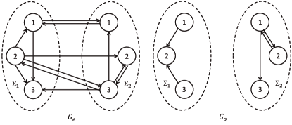
The communication graph switches periodically over the two graphs given in Fig. 1, where and , .
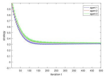
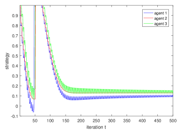
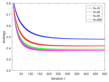
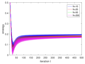
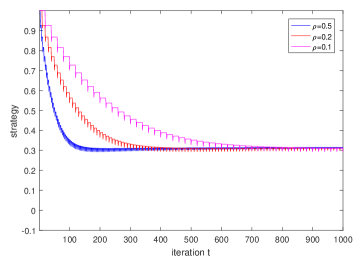
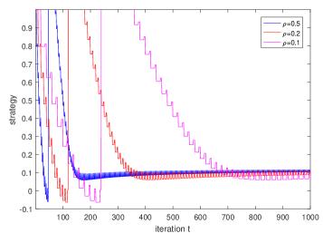
We take the number of discrete points and the compression ratio in Algorithm 1. Firstly, we illustrate the convergence of Algorithm 1. We present the trajectories of strategies in for types and under and in Fig. 2. We can see that the agents’ strategies reach consensus and converge. Fig. 3 shows strategy trajectories of agent 1 in for types and under different . We find that the limit point of converges as tends to infinity, which is consistent with Theorem 3.
Then we demonstrate the effectiveness of compression. In the communication, each agent sends -dimensional compressed strategies (8 bytes per element) and the index of those strategies (4 bytes per element) to their current neighbors. Thus, the communication data size of an iteration can be calculated by
| (21) |
| Data (kb) | ||||
|---|---|---|---|---|
| 19.92 | 9.96 | 3.98 | 1.99 | |
| 99.61 | 49.80 | 19.92 | 9.96 |
We can see that our compression considerably reduce the communication loads. Fig. 4 demonstrates the convergence of strategies in for specific types and under different with . As Fig. 4, the compression does not affect the convergence, which means that whatever we choose, Algorithm 1 remains convergent.
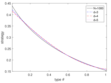
Next, we verify the approximation of the BNE generated by Algorithm 1. Here we compare the equilibrium obtained from Algorithm 1 and the equilibria obtained by polynomial approximation in [15] in Fig. 5. Compared with results by polynomial approximations, we believe that the DBNE is close to the true equilibrium.
9 Conclusion
In this paper, we proposed a distributed algorithm for seeking a continuous-type BNE in subnetwork zero-sum games. We showed that the algorithm could obtain an approximate BNE with an explicit error bound via communication-efficient computation. Our algorithm involved two main steps. In the discretization step, we established a discretized model and provided the relation between the DBNE of the discretized model and the BNE of the continuous model with the explicit error bound. Then in the communication step, we provided a novel communication scheme with a designed sparsification rule, which could effectively reduce the amount of communication and adapt well to time-varying networks, and we proved that agents could obtain unbiased estimations through such communication. Finally, we provided convergence analysis of the algorithm and its convergence rate in the considered settings.
Appendix Appendix A Proof of Lemma 3
For any and , according to L’Hospital’s rule,
Thus, by the best responses in and , for any and , there exists a strategy such that, as , Since is piecewise continuous, for any , there exists a such that, for any except for finite points and , . As , ,
| (22) |
As , (22) implies for almost every .
Appendix Appendix B Proof of Lemma 4
To estimate the BNE of with strategies in , we first convert the continuous model to the discretized model , and then estimate the error between and for strategies in .
From Assumption 2(iv), for each and , is continuous in for any , and . For any and ,
where . Note that a strategy in is a constant for the types lying in . For any and ,
| (23) | ||||
Then, according to the definition of the DBNE in (4), for any ,
| (24) |
Our purpose is to convert the term on the left hand of (24) from the discretized form to the continuous form. To get the relation between the discretized form and the continuous form, we adopt the distribution used in Definition 4. For any ,
| (25) | ||||
Due to the Lipschitz continuity of ,
| (26) | ||||
According to the Lipschitz continuity of and the compactness of , , , and , there exists a constant such that . Applying (26) to (25),
Thus, for any , (24) can be rewritten as
| (27) | ||||
where . Then applying (27) to (23), for any ,
namely , where . Similarly, for any , . Hence, a DBNE is an -BNE with .
Next, we prove that the DBNE converges to the BNE. By the zero-sum condition,
Thus, . Since is -strongly convex, for any and ,
Because for any , ,
namely . Similarly, . As and tend to infinity, tends to 0, and thus the DBNE converges to the BNE .
Appendix Appendix C Proof of Proposition 1
According to Assumption 2(vi), each agent is able to communicate with agents in once every iterations and have access to messages from every iterations, which means that can receive nonempty messages () at each entry from in iterations and nonempty messages () at each entry from in iterations. Thus, the generated graph sequences satisfy Proposition 1 with and .
Appendix Appendix D Proof of Lemma 5
Due to Jensen’s inequality,
At time , denote the last time agent receive nonempty messages from its rivals at the entry () by . From Proposition 1(b), . For any ,
Appendix Appendix E Proof of Proposition 2
For any and , denote the projection by and . Since is convex, for . Therefore, for any .
Thus, is convex. Moreover,
Similarly, . Therefore, is -Lipschitz continuous in .
By the properties of projection, for any . Then
Thus, is a subgradient of .
Fix . Denote the optimal strategy of by when adopts , which satisfies for . For any ,
Then we obtain a similar result for . Therefore, for , the minimizer of in lies in .
References
- [1] K. Akkarajitsakul, E. Hossain, and D. Niyato, Distributed resource allocation in wireless networks under uncertainty and application of Bayesian game, IEEE Communications Magazine, 49 (2011), pp. 120–127.
- [2] D. Alistarh, D. Grubic, J. Li, R. Tomioka, and M. Vojnovic, QSGD: Communication-efficient SGD via gradient quantization and encoding, Advances in Neural Information Processing Systems, 30 (2017), pp. 1709–1720.
- [3] S. Athey, Single crossing properties and the existence of pure strategy equilibria in games of incomplete information, Econometrica, 69 (2001), pp. 861–889.
- [4] T. Başar and S. Li, Distributed computation of Nash equilibria in linear-quadratic stochastic differential games, SIAM Journal on Control and Optimization, 27 (1989), pp. 563–578.
- [5] J. Bernstein, Y.-X. Wang, K. Azizzadenesheli, and A. Anandkumar, signSGD: Compressed optimisation for non-convex problems, in International Conference on Machine Learning, PMLR, 2018, pp. 560–569.
- [6] U. Bhaskar, Y. Cheng, Y. K. Ko, and C. Swamy, Hardness results for signaling in Bayesian zero-sum and network routing games, in Proceedings of the 2016 ACM Conference on Economics and Computation, 2016, pp. 479–496.
- [7] K. Cai and H. Ishii, Average consensus on arbitrary strongly connected digraphs with time-varying topologies, IEEE Transactions on Automatic Control, 59 (2014), pp. 1066–1071.
- [8] A. Chakraborti, D. Challet, A. Chatterjee, M. Marsili, Y. C. Zhang, and B. K. Chakrabarti, Statistical mechanics of competitive resource allocation using agent-based models, Physics Reports-Review Section of Physics Letters, 552 (2015), pp. 1–25.
- [9] G. Chen, K. Cao, and Y. Hong, Learning implicit information in Bayesian games with knowledge transfer, Control Theory and Technology, 18 (2020), pp. 315–323.
- [10] Y. Chen, A. Hashemi, and H. Vikalo, Decentralized optimization on time-varying directed graphs under communication constraints, in ICASSP 2021-2021 IEEE International Conference on Acoustics, Speech and Signal Processing (ICASSP), IEEE, pp. 3670–3674.
- [11] X. Fang, G. Wen, J. Zhou, and W. X. Zheng, Distributed adaptive Nash equilibrium seeking over multi-agent networks with communication uncertainties, in 2021 60th IEEE Conference on Decision and Control (CDC), pp. 3387–3392.
- [12] M. Fey, Rent-seeking contests with incomplete information, Public Choice, 135 (2008), pp. 225–236.
- [13] B. Gharesifard and J. Cortés, Distributed convergence to Nash equilibria in two-network zero-sum games, Automatica, 49 (2013), pp. 1683–1692.
- [14] M. Großhans, C. Sawade, M. Brückner, and T. Scheffer, Bayesian games for adversarial regression problems, in International Conference on Machine Learning, PMLR, pp. 55–63.
- [15] S. Guo, H. Xu, and L. Zhang, Existence and approximation of continuous Bayesian Nash equilibria in games with continuous type and action spaces, SIAM Journal on Optimization, 31 (2021), pp. 2481–2507.
- [16] W. Guo, M. I. Jordan, and T. Lin, A variational inequality approach to Bayesian regression games, in 2021 60th IEEE Conference on Decision and Control (CDC), IEEE, pp. 795–802.
- [17] J. C. Harsanyi, Games with incomplete information played by “Bayesian” players, I–III part I. the basic model, Management science, 14 (1967), pp. 159–182.
- [18] I. Hogeboom-Burr and S. Yüksel, Comparison of information structures for zero-sum games and a partial converse to Blackwell ordering in standard Borel spaces, SIAM Journal on Control and Optimization, 59 (2021), pp. 1781–1803.
- [19] L. Huang and Q. Zhu, Convergence of Bayesian Nash equilibrium in infinite Bayesian games under discretization, (2021), https://arxiv.org/abs/2102.12059.
- [20] S. Huang, J. Lei, Y. Hong, and U. V. Shanbhag, No-regret distributed learning in two-network zero-sum games, in 2021 60th IEEE Conference on Decision and Control (CDC), pp. 924–929.
- [21] V. Krishna, Auction Theory, Academic press, 2009.
- [22] S. Lakshmivarahan and K. S. Narendra, Learning algorithms for two-person zero-sum stochastic games with incomplete information: A unified approach, SIAM Journal on Control and Optimization, 20 (1982), pp. 541–552.
- [23] J. Lei, H.-F. Chen, and H.-T. Fang, Asymptotic properties of primal-dual algorithm for distributed stochastic optimization over random networks with imperfect communications, SIAM Journal on Control and Optimization, 56 (2018), pp. 2159–2188.
- [24] L. Li, C. Langbort, and J. Shamma, An LP approach for solving two-player zero-sum repeated Bayesian games, IEEE Transactions on Automatic Control, 64 (2018), pp. 3716–3731.
- [25] Y. Lou, Y. Hong, L. Xie, G. Shi, and K. H. Johansson, Nash equilibrium computation in subnetwork zero-sum games with switching communications, IEEE Transactions on Automatic Control, 61 (2015), pp. 2920–2935.
- [26] A. Meirowitz, On the existence of equilibria to Bayesian games with non-finite type and action spaces, Economics Letters, 78 (2003), pp. 213–218.
- [27] P. R. Milgrom and R. J. Weber, Distributional strategies for games with incomplete information, Mathematics of Operations Research, 10 (1985), pp. 619–632.
- [28] A. Nedić and A. Olshevsky, Distributed optimization over time-varying directed graphs, IEEE Transactions on Automatic Control, 60 (2015), pp. 601–615.
- [29] B. T. Polyak, Introduction to Optimization, Optimization Software, New York, 1987.
- [30] S. S. Ram, A. Nedić, and V. V. Veeravalli, Incremental stochastic subgradient algorithms for convex optimization, SIAM Journal on Optimization, 20 (2009), pp. 691–717.
- [31] B. Rynne and M. A. Youngson, Linear Functional Analysis, Springer Science & Business Media, 2007.
- [32] F. Sattler, S. Wiedemann, K.-R. Müller, and W. Samek, Robust and communication-efficient federated learning from non-i.i.d. data, IEEE Transactions on Neural Networks and Learning Systems, 31 (2020), pp. 3400–3413.
- [33] M. Sola and G. M. Vitetta, Demand-side management in a smart micro-grid: A distributed approach based on Bayesian game theory, in 2014 IEEE International Conference on Smart Grid Communications (SmartGridComm), pp. 656–661.
- [34] T. Ui, Bayesian Nash equilibrium and variational inequalities, Journal of Mathematical Economics, 63 (2016), pp. 139–146.
- [35] J. Wangni, J. Wang, J. Liu, and T. Zhang, Gradient sparsification for communication-efficient distributed optimization, Advances in Neural Information Processing Systems, 31 (2018).
- [36] G. Xu, G. Chen, H. Qi, and Y. Hong, Efficient algorithm for approximating Nash equilibrium of distributed aggregative games, IEEE Transactions on Cybernetics, (2022), pp. 1–13.
- [37] Z. Yu, D. W. C. Ho, D. Yuan, and J. Liu, Distributed stochastic constrained composite optimization over time-varying network with a class of communication noise, IEEE Transactions on Cybernetics, (2021), pp. 1–13.
- [38] Y. Zeng, E. Gunawan, and Y. L. Guan, Distributed power allocation for network MIMO with a Bayesian game-theoretic approach, in 2011 8th International Conference on Information, Communications & Signal Processing, pp. 1–5.