TSFool: Crafting Highly-imperceptible Adversarial Time Series through Multi-objective Black-box Attack to Fool RNN Classifiers

Abstract

Neural network (NN) classifiers are vulnerable to adversarial attacks. Although the existing gradient-based attacks achieve state-of-the-art performance in feed-forward NNs and image recognition tasks, they do not perform as well on time series classification with recurrent neural network (RNN) models. This is because the cyclical structure of RNN prevents direct model differentiation and the visual sensitivity of time series data to perturbations challenges the traditional local optimization objective of the adversarial attack. In this paper, a black-box method called TSFool is proposed to efficiently craft highly-imperceptible adversarial time series for RNN classifiers. We propose a novel global optimization objective named Camouflage Coefficient to consider the imperceptibility of adversarial samples from the perspective of class distribution, and accordingly refine the adversarial attack as a multi-objective optimization problem to enhance the perturbation quality. To get rid of the dependence on gradient information, we also propose a new idea that introduces a representation model for RNN to capture deeply embedded vulnerable samples having otherness between their features and latent manifold, based on which the optimization solution can be heuristically approximated. Experiments on 10 UCR datasets are conducted to confirm that TSFool averagely outperforms existing methods with a 46.3% higher attack success rate, 87.4% smaller perturbation and 25.6% better Camouflage Coefficient at a similar time cost.

I Introduction

Advanced NN classifiers can automatically extract key features from datasets and generate accurate predictions. However, researchers have found that such models are vulnerable to adversarial attacks [1], which means imperceptible perturbations added to the input can cause the output change significantly [2]. A rich body of adversarial attack technologies has been proposed to deal with this problem by generating adversarial samples to enhance the robustness of the models. For instance, the commonly used methods based on model gradient [3, 5, 4, 6] have achieved impressive performance in the context of feed-forward NN classifiers and image recognition tasks.

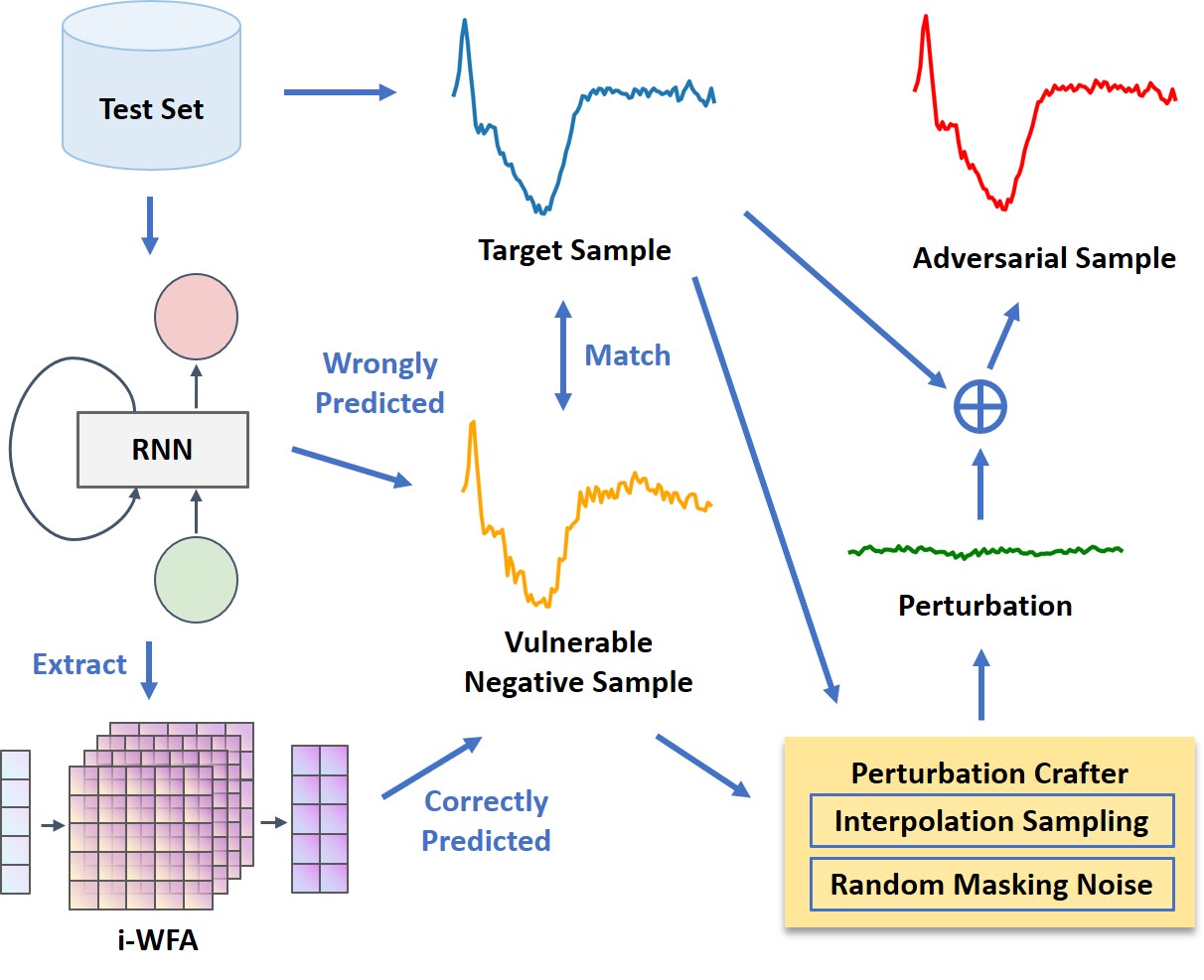
Figure 1: The sketch map of TSFool. With the representation model i-WFA extracted from RNN, the vulnerable sample having otherness between features and latent manifold is captured. Then the target is matched and accordingly perturbed through two steps namely interpolation sampling and noise adding.

However, those gradient-based adversarial attacks always assume that the target model is directly differentiable, while the unique time recurrent structure of RNN prevents such computation [7]. On the other hand, existing attacks always follow a traditional local optimization objective to minimize the perturbation amount for every single sample. Nevertheless, for time series which is far more visually sensitive to perturbation than image data, the reasonability and effectiveness of this approach that seems to be tailored for image data are questionable. To date, while time series classification is implemented in various real-world safety-critical applications ranging from health care to food safety [8], and RNN is commonly adopted by the state-of-the-art models in such areas [9], the existing methods do not work well to generate adversarial time series for RNN classifiers. Some efforts have been made to deal with this problem, yet the idea to make RNN differentiable by cyclical computational graph unfolding [7] is not efficient and scalable enough in practice, and the black-box attacks relying on the adversarial transferability to avoid RNN like [8] only get very limited success.

In this paper, we propose a black-box method named TSFool to efficiently craft highly-imperceptible adversarial time series for RNN classifiers. With an argument that the local optimal perturbation defined under the traditional objective does not always lead to imperceptible adversarial attacks, we propose a novel global optimization objective named Camouflage Coefficient, and add it to make the adversarial attack a multi-objective optimization problem. In this way, we take the relative position between adversarial samples and class clusters into consideration, to measure the imperceptibility of adversarial samples from the perspective of class distribution. To heuristically and efficiently approximate the optimization solution, we capture the misclassified samples deeply embedded in specific positive classes as the guide, and accordingly pick target samples to perturb in the direction of their interpolation to imperceptibly cross the classification hyperplane. Given the RNN without gradient information available, we propose a new black-box idea to introduce a representation model constructed based on output predictions only, which can fit the manifold hyperplane of a classifier but distinguish samples by their features like humans, to find the guide sample having otherness between latent manifold and features.

With five basic or state-of-the-art adversarial attacks as the benchmark, our evaluation on 10 UCR time series datasets and LSTM classifiers demonstrates that TSFool has significant advantages in effectiveness and imperceptibility under considerable efficiency. Specifically, TSFool averagely outperforms the benchmark methods with a 46.3% higher attack success rate, 87.4% smaller local perturbation and 25.6% better global Camouflage Coefficient.

II Background and Related Work

II-A Basics of Adversarial Attack

The concept of adversarial attack is firstly introduced by [1], in which an adversarial sample $\vec{x}^{*}$ crafted from a legitimate sample $\vec{x}$ is defined by an optimization problem:

$$\vec{x}^{*}=\vec{x}+\delta_{\vec{x}}=\vec{x}+\text{min}\hskip 1.00006pt\|\vec{z}\|\text{ s.t.}\hskip 1.49994ptf(\vec{x}+\vec{z})\neq f(\vec{x})$$ (1)

where $f:\mathbb{R}^{n}\rightarrow\vec{y}$ is the target classifier and $\delta_{\vec{x}}$ is the smallest perturbation according to a norm appropriate for the input domain. Since exactly solving this problem by an optimization method is time-consuming [4] and not always possible, especially in NNs with complex non-convexity and non-linearity [7], the common practice is to find the approximative solutions to estimate adversarial examples.

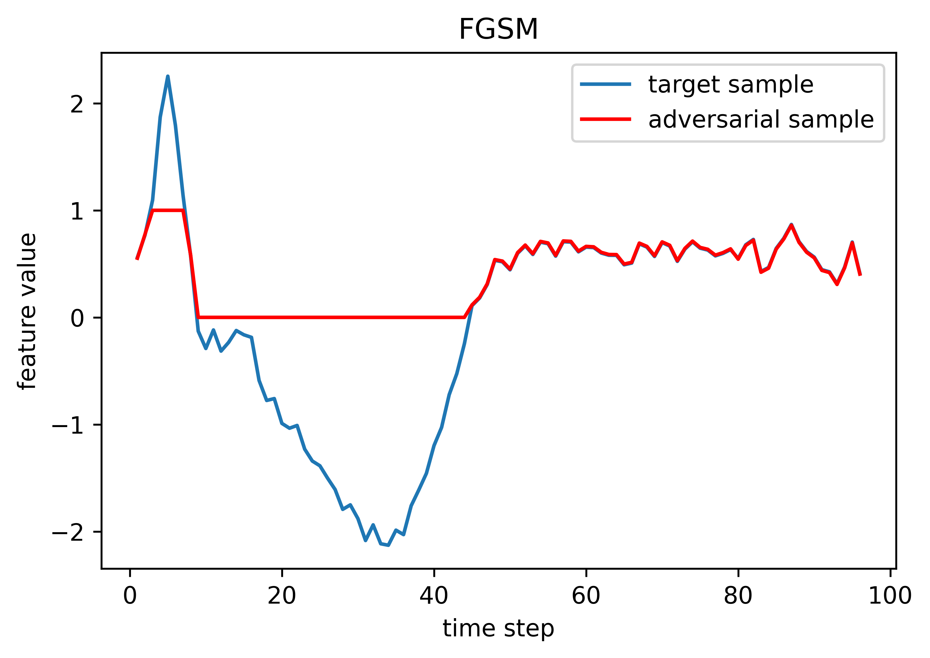
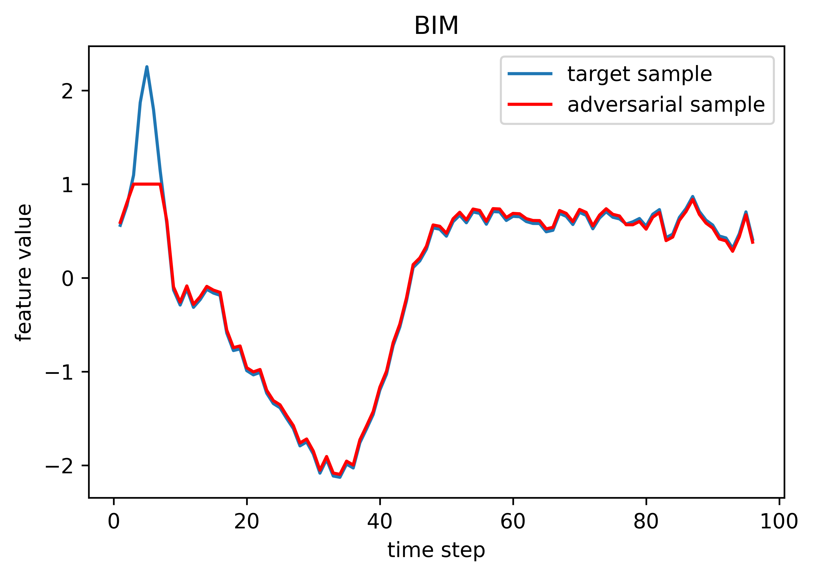
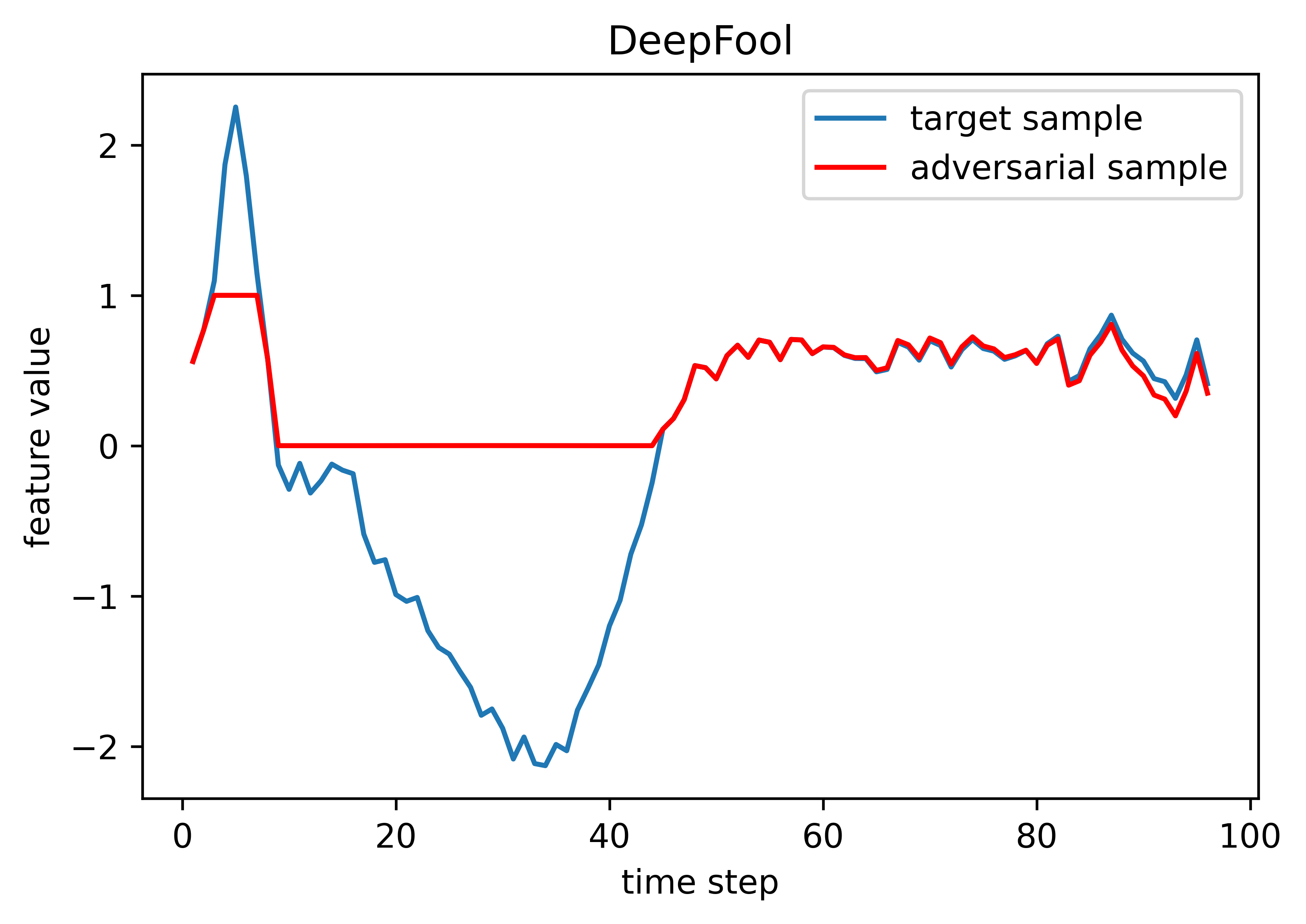
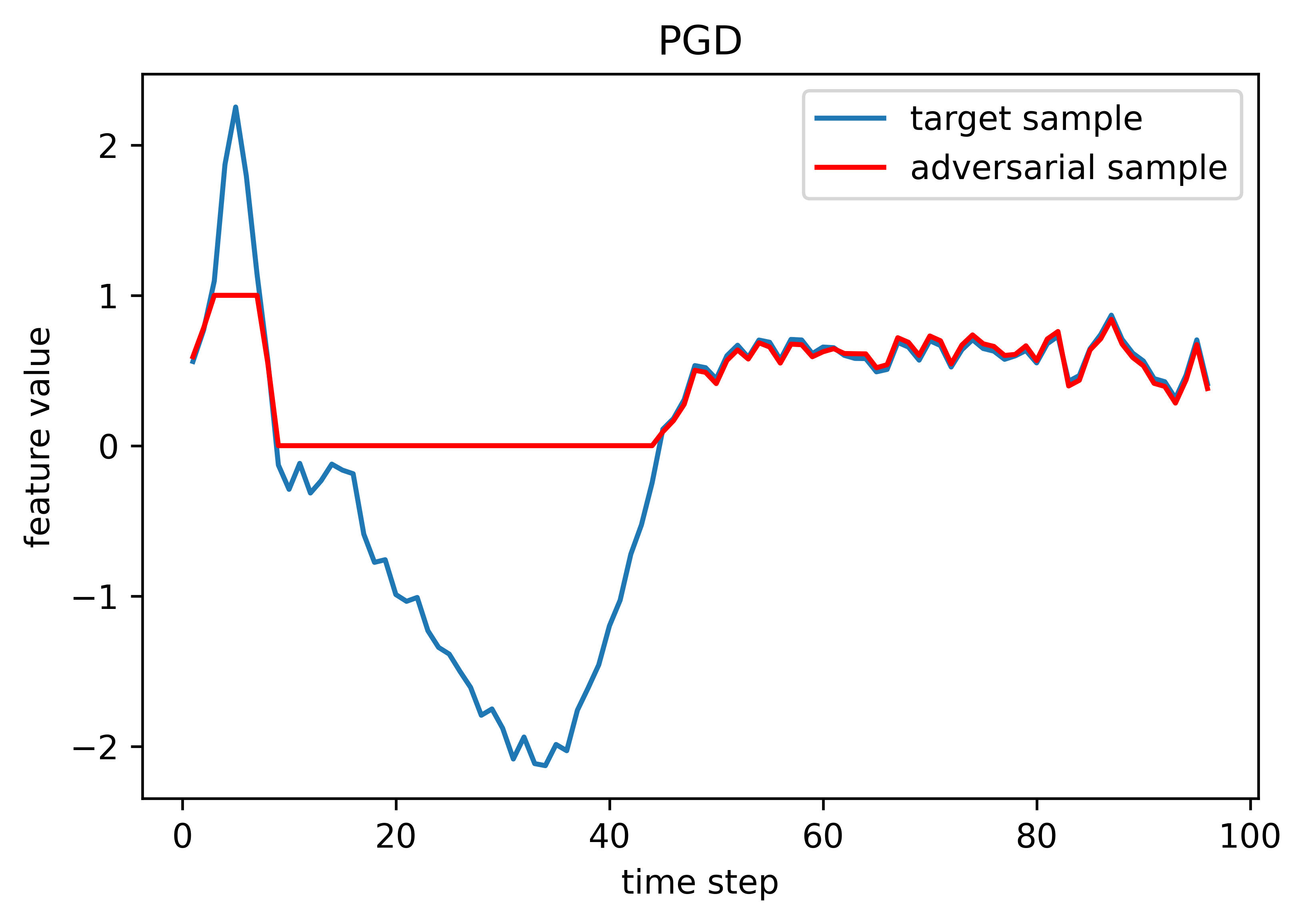
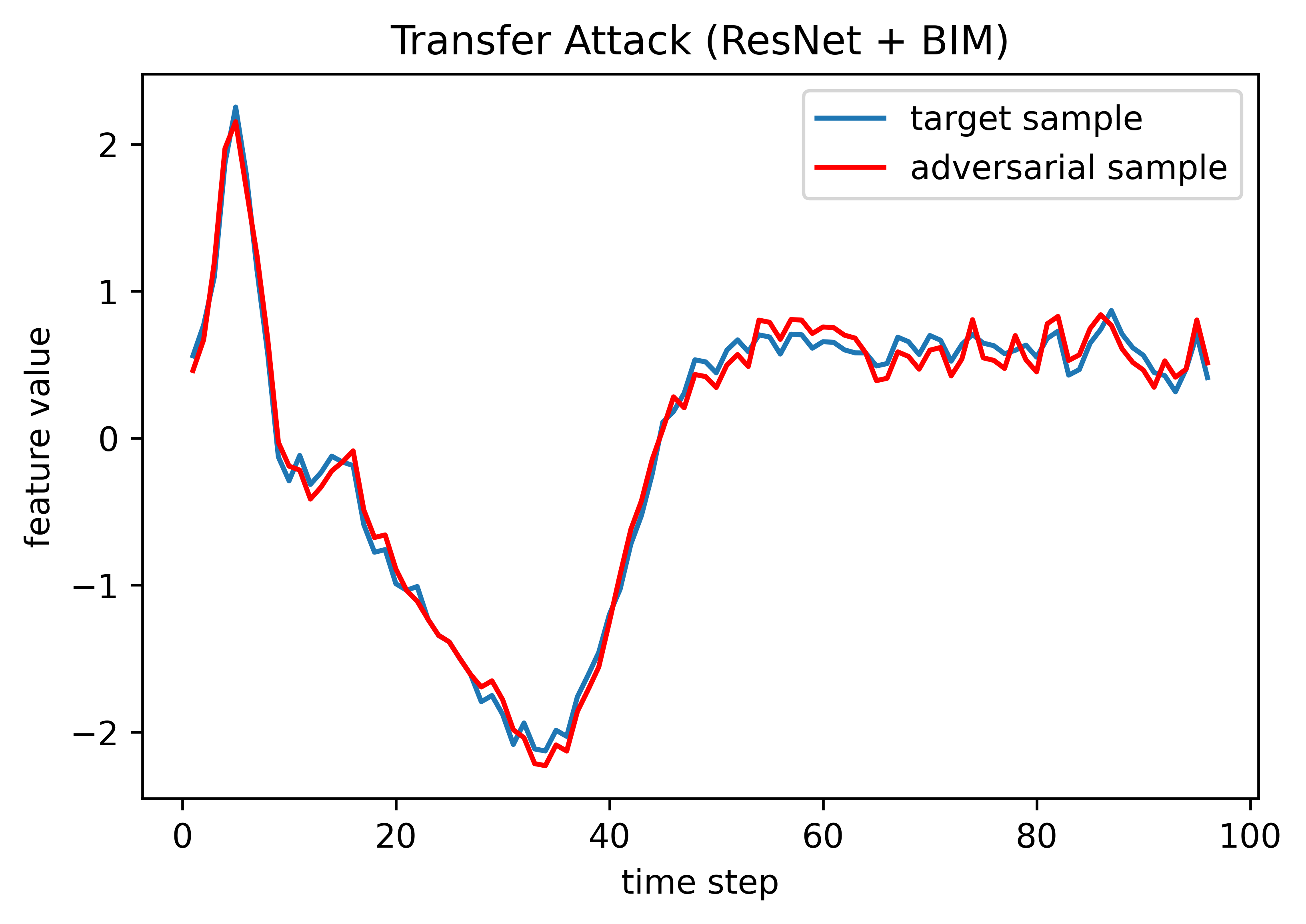
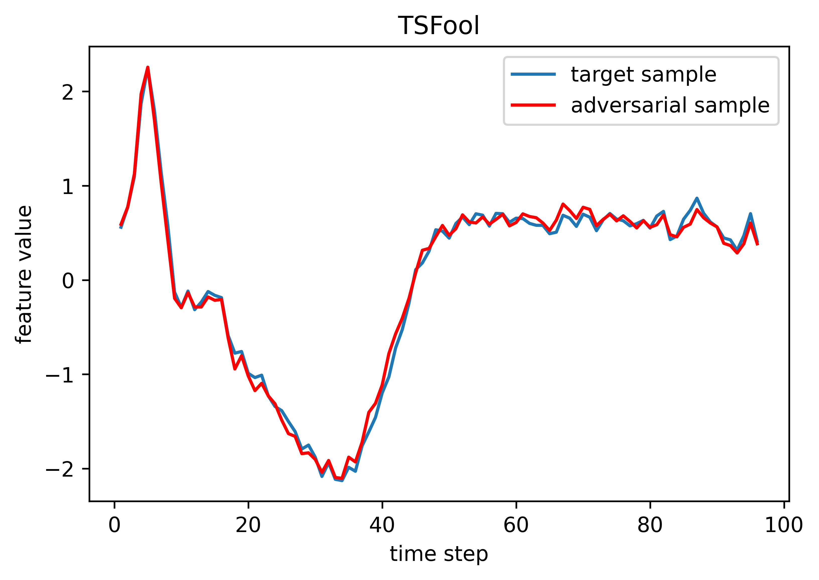
Figure 2: The figures show the instances of adversarial attacks through TSFool and the benchmark methods in a UCR dataset named ECG200. The unsatisfying results of FGSM, DeepFool and PGD are similar with only slight differences in the latter time steps. BIM performs better than them, but still heavily changes several features. The transfer attack basically achieves small perturbation, while TSFool realizes the most imperceptible attack here.

The most commonly used adversarial attacks to date are gradient-based methods under white-box setting [10], which means all the information of the target classifier is available and the perturbation is guided by the differentiating functions defined over model structure and parameters. For instance, the fast gradient sign method (FGSM) [3] implements the perturbation according to the gradient of cost function $\mathcal{L}$ with respect to the input $\vec{x}$:

$$\delta_{\vec{x}}=\varepsilon\hskip 1.00006pt\text{sign}(\nabla_{\vec{x}}\hskip 1.49994pt\mathcal{L}(f,\vec{x},\vec{y}))$$ (2)

where $\varepsilon$ denotes the magnitude of the perturbation. Then a following work named basic iterative method (BIM) [5] extends FGSM by applying it iteratively with a small step size and clipping the obtained samples after each step. On the other hand, the DeepFool [4] introduces a greedy idea to determine the perturbation direction of specific samples according to their closest classification hyperplane. Both of them are expected to make the perturbation smaller. Finally, as one of the most frequently used state-of-the-art benchmark [11], the projected gradient descent attack (PGD) [6] can be viewed as a further variant of FGSM. It crafts samples iteratively by getting the perturbation through FGSM and projecting it to the $\epsilon$-ball of input at each step. To be specific, given $\vec{x}^{t}$ as the intermediate input from step $t$, the PGD updates as:

$$\vec{x}^{t+1}=\Pi_{\epsilon}\left\{\hskip 1.49994pt\vec{x}^{t}+\varepsilon\cdot\text{sign}(\nabla_{\vec{x}}\hskip 1.49994pt\mathcal{L}(f,\vec{x}^{t},\vec{y})),\hskip 2.5pt\vec{x}\hskip 1.49994pt\right\}$$ (3)

II-B Drawbacks of Existing Methods in RNN and Time Series

While the existing methods achieve great success on feed-forward NNs and image data, it has not carried over to RNN-based time series classification. There are two main reasons for this dilemma. For one thing, the presence of cyclical computations in the architecture of RNN prevents direct model differentiation [7], which means the full gradient information is no longer available through the chain rule. This problem seriously challenges the effectiveness of all the gradient-based methods. For another, in practice, image data can tolerate respectively considerable perturbation without being noticed by humans, while time series data are so visually sensitive to the perturbation that it is more difficult to ensure their imperceptibility [9]. This problem exposes the drawback of existing methods in perturbation quality control.

An intuitive solution for the first problem is to make the model differentiable through cyclical computational graph unfolding technology to fit the gradient-based methods [7]. However, as the length of the time series is considerable in most real-world cases, the practical efficiency and scalability of the unfolding computation cannot be guaranteed. Another idea is to craft adversarial time series based on other acyclic NN models built for the same task, and then rely on the transferability of the adversarial sample to implement black-box attack [8]. Unfortunately, although the transfer attack avoids the difficulty of specialized design for RNN and is expected to realize small perturbation, its effectiveness in practice is unpredictable (as to be shown in our experiment). Besides, for the perturbation quality, it is surprising that the only current measure of time series data is the number of time steps perturbed [7], while the specific perturbation amount which is even more important is still absent. All in all, the problems brought by the recurrent structure of RNN and perturbation sensitivity of time series remain to be further explored.

III Motivation

III-A Reconsider Highly-imperceptible Adversarial Sample

The sensitivity of time series data prompts us to rethink the imperceptibility of perturbation. Firstly, existing methods always implement perturbations to all of the test data, while according to the specific class distribution, there must be individuals among them that are easier or harder to be perturbed respectively. Without taking this difference into account and picking target samples appropriately, it is almost impossible for the attack method to stably control the perturbation amount by itself. on the contrary, it has to heavily depend on the specific dataset. Secondly, we argue that the approximation to the optimal perturbation $\delta_{\vec{x}}$ in (1) does not always lead to a highly-imperceptible adversarial attack, while all of the existing methods view it as the basic target. This is because when we jump out of a single sample and consider it from the perspective of class distribution, it can be found that even the minimal perturbation is not necessarily the most imperceptible one. For instance, in Fig. 3, the adversarial sample $x_{1}$ is generated from $x_{0}$ through a minimal perturbation that crosses the closest classification hyperplane like DeepFool, while another adversarial sample $x_{2}$ is obviously more dangerous as it is visually closer to and even belong to the original class. Such cases are commonly seen in our experiments.

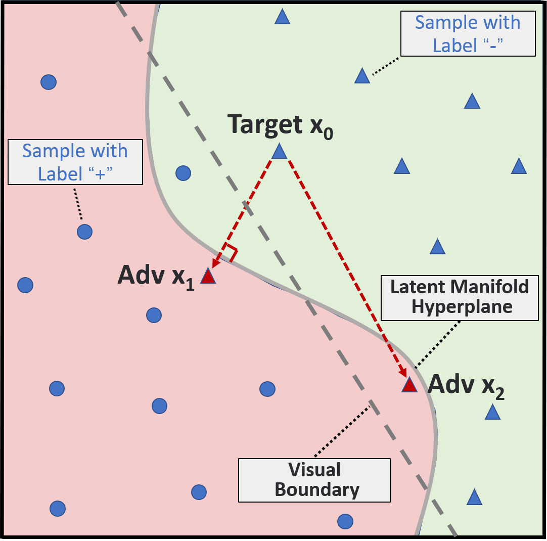
Figure 3: An intuitive instance that the minimal perturbation (i.e. $\|x_{1}-x_{0}\|$) is not necessarily the most imperceptible in the global perspective. Notice that the visual boundary and latent manifold hyperplane are different classification boundaries respectively from the human and the learned model.

This inspired us to introduce a new definition of the quality of an adversarial sample from the global view. Given a $k$-class classification task and the label $i,j\in\{0,1,...,k-1\}$, $\mathcal{X}_{i}$ is the set of all the samples belonging to class $i$ in the test set. For $\vec{x}\in\mathcal{X}_{i}$ and the corresponding adversarial sample $\vec{x}^{*}$ which is wrongly predicted as $f(\vec{x}^{*})=j\hskip 3.99994pt(j\neq i)$, the Camouflage Coefficient $\mathcal{C}$ of $\vec{x}^{*}$ is defined as:

$$\mathcal{C}({\vec{x}^{*}})=\frac{\|\vec{x}^{*}-\vec{m}_{i}\|/d_{i}}{\hskip 0.50003pt\|\vec{x}^{*}-\vec{m}_{j}\|/d_{j}}$$ (4)

where $m_{i}$ is the center of mass of class $i$ which is also built in the form of a legal sample:

$$m_{i}=\frac{1}{|\mathcal{X}_{i}|}\sum_{x_{t}\in\mathcal{X}_{i}}x_{t}$$ (5)

and $d_{i}$ is the average norm distance between $m_{i}$ and all the samples in $\mathcal{X}_{i}$, which is used to eliminate the potential bias from the different cluster sizes of the two classes:

$$d_{i}=\frac{1}{|\mathcal{X}_{i}|}\sum_{x_{t}\in\mathcal{X}_{i}}\|x_{t}-m_{i}\|$$ (6)

Just as the saying goes, “the best place to hide a leaf is in the woods”. The Camouflage Coefficient represents the proportion of the relative distance between adversarial sample $\vec{x}^{*}$ and the original class to the relative distance between $\vec{x}^{*}$ and the class to which it is misclassified. As a result, the measure can reveal to what extent an adversarial sample can hide in the original class without being noticed. The smaller the value, the higher the global imperceptibility of the adversarial sample. While if the value exceeds one, the attack fails from the perspective of imperceptibility. Because in this case, the misclassification of the adversarial sample is no longer surprising as it already looks more like the samples in that wrong class instead of the original class. In our approach, we introduce the Camouflage Coefficient as another optimization objective along with (1) to craft highly-imperceptible adversarial samples considering local perturbation and global camouflage at the same time.

III-B Adversarial Attack through Multi-objective Perturbation

After adding the Camouflage Coefficient, the adversarial attack becomes a multi-objective optimization problem. Just as the existing methods, considering the efficiency, we do not solve it directly, but find the approximate solution in a logical and practical way. Separately speaking, to optimize (4), we can just make $\vec{x}^{*}$ closer to the $\vec{m}_{i}$, which also means farther away from the $\vec{m}_{j}$ in general. And to approximate the objective in (1), perturbing in the direction of the closest classification hyperplane is proven to be a successful approach in DeepFool. So as a compromise to take them into account together, a reasonable idea is to cross a hyperplane that is relatively near the target sample $\vec{x}$ on an appropriate place that is relatively close to the $\vec{m}_{i}$.

To realize this idea in practice, we can find a sample $\vec{x}_{v}$ from $\mathcal{X}_{i}$ which is misclassified to class $j$ but deeply embedded in class $i$ as a guide, and accordingly pick a correctly classified sample that is the closest to $\vec{x}_{v}$ in class $i$ as the target $\vec{x}$. Then when we perturb $\vec{x}$ in the direction of $\vec{x}_{v}$ to cross the classification hyperplane between them, we can not only acquire a considerable value of Camouflage Coefficient as the $\vec{x}_{v}$ itself is a sample embedded closer to $\vec{m}_{i}$ than to $\vec{m}_{j}$, but also expect the hyperplane is relatively a close one to $\vec{x}$ as this sample is the closest to $\vec{x}_{v}$ among class $i$. In this way, the $\vec{x}$ is not perturbed to be adversarial along the shortest path, but the more imperceptible one under the multi-objective definition. We define the $\vec{x}_{v}$ and $\vec{x}$ respectively as Vulnerable Negative Sample (VNS) and Target Positive Sample (TPS), with which the perturbation can be denoted as:

$$\delta_{\vec{x}}=\lambda_{\varepsilon}\|\vec{x}_{v}-\vec{x}\|+\vec{x}_{\varepsilon}$$ (7)

where $\lambda_{\varepsilon}\|\vec{x}_{v}-\vec{x}\|$ is the maximum interpolation that makes $\vec{x}$ approach $\vec{x}_{v}$ under a given step size $\varepsilon$ without changing its prediction result, and $\vec{x}_{\varepsilon}$ is a micro random noise under the same $\varepsilon$ added to cross the classification hyperplane.

III-C Capture Vulnerable Sample by Manifold Hypothesis

Now the only problem left is how to capture the VNS, and our idea to solve it comes from the manifold hypothesis. It is one of the generally accepted explanations for the effectiveness of NNs, which holds that many high-dimensional data in the real world are actually distributed along low-dimensional manifolds embedded in the high-dimensional space [12]. This explains why NNs can find latent key features as complex functions of a large number of original features in the data. And it is through learning the manifold of the latent key features of training data that NNs can realize manifold interpolation between input samples and generate accurate predictions of unseen samples [13]. So what matters in NN classification is how to distinguish the latent manifolds instead of the original features of samples with different labels.

However, due to the limitation of sampling technologies and human cognitive ability, practical label construction and model evaluation usually have to rely on a specific form of data with features in a high-dimensional space. Accordingly, a possible explanation for the existence of the adversarial sample is that, the features of input data cannot always fully and visually reflect the latent manifold, which makes it possible for the samples considered to be similar in features to have dramatically different latent manifolds. As a consequence, even a small perturbation in human cognition added to a correctly predicted sample may completely change the perception of NN to its latent manifold, and result in a significantly different prediction result.

So if there is a kind of representation model that can imitate the mechanism of a specific NN classifier to predict input data, but distinguish different inputs by their features in the original high-dimensional space just like a human, then it can be introduced to capture the otherness between the latent manifold and features of specific samples. Such otherness can serve as a guide to capture the VNS. Specifically, when the prediction of the representation model is correct while that of the NN classifier is wrong, it means that compared with other samples that are similar in features and belong to the same class in fact, the current sample is perceived by NN as a different latent manifold, so as to be wrongly predicted. It is obvious that such samples meet the definition of VNS.

IV Approach

Based on the ideas in section III, we propose a black-box approach named TSFool to efficiently craft highly-imperceptible adversarial time series for RNN classifiers. The sketch map is shown in Fig. 1. In this section, we detailed describe the establishment of the representation model and the crafting of perturbation including the capture of VNS and the implementation of interpolation sampling and random masking noise.

IV-A Establish Representation Model

To model the special recurrent computation of RNN, we introduce weighted finite automaton (WFA) [14] that can imitate the execution of RNN based on its hidden state updated at each time step. Nevertheless, WFA also relies on existing clustering methods like $k\text{-}means$ to abstract input data, while another requirement of the representation model is to distinguish different inputs directly by original features as a human. So we improve WFA by changing its input from data clusters to domain intervals.

An Intervalized Weighted Finite Automaton (i-WFA) extracted from a $k$-class RNN classifier $\mathcal{N}$ is defined as a tuple $\mathcal{A}=(Z,S,\mathcal{I},(E_{\zeta})_{\zeta\in Z},\mathcal{T})$, where $Z$ is a finite set of intervals that covers the whole input domain, $S$ is a finite set of states abstracted from the hidden states of $\mathcal{N}$, $\mathcal{I}$ is the initial state vector of dimension $|S|$, and $\mathcal{T}$ is the probabilistic output matrix with size $|S|\times k$. For each interval $\zeta\in Z$, the corresponding probabilistic transfer matrix $E_{\zeta}$ with size $|S|\times|S|$ is built according to the hidden transfer of all the samples having features that fall into this interval. In the execution of i-WFA, the $\mathcal{I}$ is iteratively updated to represent the current state with the transfer under different inputs imitated by the corresponding $E_{\zeta}$ at each time step, followed by the $\mathcal{T}$ to imitate the computation of probabilistic predictions finally.

For instance, in a two-class classification task, given an input time series $X=[x_{1},x_{2},x_{3}]_{(x_{i}\in\zeta_{i})}$ with three time steps and the input $x_{i}$ of each time step falls into the input intervals $\zeta_{i}$. Given $S=[s_{0},s_{1},s_{2}]$, an initial $\mathcal{I}=\left[\hskip 3.00003pt1\hskip 6.99997pt0\hskip 6.99997pt0\hskip 3.00003pt\right]$,

$$E_{\zeta_{1}}=\left[\begin{array}[]{ccc}1/4&0&3/4\\ 0&0&0\\ 0&0&0\end{array}\right],\hskip 3.00003ptE_{\zeta_{2}}=\left[\begin{array}[]{ccc}1/4&1/4&1/2\\ 1&0&0\\ 1/2&1/2&0\end{array}\right],$$

$$E_{\zeta_{3}}=\left[\begin{array}[]{ccc}0&1&0\\ 0&1/4&3/4\\ 1/4&1/2&1/4\end{array}\right],\hskip 3.00003ptand\hskip 3.00003pt\mathcal{T}=\left[\begin{array}[]{cc}1/2&1/2\\ 0&1\\ 3/4&1/4\end{array}\right],$$

the execution of i-WFA can be illustrated as:

$$\mathcal{I}\cdot\left(\prod_{i=1}^{|X|}E_{\zeta_{i}}\right)\cdot\mathcal{T}=\mathcal{I}\cdot E_{\zeta_{1}}\cdot E_{\zeta_{2}}\cdot E_{\zeta_{3}}\cdot\mathcal{T}\hskip 60.00009pt$$

$$=\left[\hskip 3.00003pt1\hskip 6.99997pt0\hskip 6.99997pt0\hskip 3.00003pt\right]\cdot\left[\begin{array}[]{ccc}1/4&0&3/4\\ 0&0&0\\ 0&0&0\end{array}\right]\cdot E_{\zeta_{2}}\cdot E_{\zeta_{3}}\cdot\mathcal{T}$$

$$\hskip 8.00003pt=\left[\hskip 3.00003pt1/4\hskip 6.99997pt0\hskip 6.99997pt3/4\hskip 3.00003pt\right]\cdot\left[\begin{array}[]{ccc}1/4&1/4&1/2\\ 1&0&0\\ 1/2&1/2&0\end{array}\right]\cdot E_{\zeta_{3}}\cdot\mathcal{T}$$

$$\hskip 8.00003pt=\left[\hskip 3.00003pt7/16\hskip 6.99997pt7/16\hskip 6.99997pt1/8\hskip 3.00003pt\right]\cdot\left[\begin{array}[]{ccc}0&1&0\\ 0&1/4&3/4\\ 1/4&1/2&1/4\end{array}\right]\cdot\mathcal{T}$$

$$\hskip 3.99994pt=\left[\hskip 3.00003pt1/32\hskip 6.99997pt39/64\hskip 6.99997pt23/64\hskip 3.00003pt\right]\cdot\left[\begin{array}[]{cc}1/2&1/2\\ 0&1\\ 3/4&1/4\end{array}\right]\hskip 20.00003pt$$

$$\hskip 16.00008pt=\left[\hskip 3.00003pt73/256\hskip 6.99997pt183/256\hskip 3.00003pt\right],\hskip 110.00017pt$$

where the first operators updated are the current states of i-WFA with the same size of $\mathcal{I}$ and elements summing to one, and the probabilistic output is just in the form of the original classifier. Such i-WFA can also be visualized as Fig. 4.

Figure 4: The visualization of the given i-WFA instance.

Algorithm 1 Establishment of i-WFA

Input: RNN $\mathcal{N}=(X,Y,H,f,g)$, Test Set $\mathcal{X}$, Hyper-parameters $K$, $T$ and $F$
Output: i-WFA $\mathcal{A}=(Z,S,\mathcal{I},(E_{\zeta})_{\zeta\in Z},\mathcal{T})$

1:  Initialize $Z\leftarrow[]$, $S^{\prime}\leftarrow[]$, $S\leftarrow[]$, $E\leftarrow[]$, $\mathcal{T}\leftarrow[]$

2:  $d\leftarrow\textit{ImperceptibleDistance}(\mathcal{X},F)$

3:  $\mathcal{X}^{\prime}\leftarrow\textit{FeaturesNormalization}(\mathcal{X})$

4:  while $X^{\prime}\in\mathcal{X}^{\prime}$ do

5:     while $x^{\prime}\in X^{\prime}$ do

6:        $\zeta\leftarrow\textit{floor}(x^{\prime})\times d$

7:        $Z.\textit{add}(\zeta)$

8:     end while

9:  end while

10:  while $X\in\mathcal{X}$ do

11:     $S^{\prime\prime}\leftarrow[g(f^{(i)}(X))]_{i=0}^{|X|}$

12:     $S^{\prime}.\textit{extend}(S^{\prime\prime})$

13:  end while

14:  while $s^{\prime}\in S^{\prime}$ do

15:     $s_{\textit{pred}}\leftarrow\textit{argsort}(-s^{\prime})[:K]$

16:     $s_{\textit{conf}}\leftarrow\textit{floor}((-\textit{sort}(-s^{\prime}[:K])\times T)$

17:     $s\leftarrow\textit{concat}(s_{\textit{pred}},s_{\textit{conf}})$

18:     $S.\textit{add}(s)$

19:  end while

20:  $\mathcal{I}\leftarrow\textit{zeros}(|S|+1)$

21:  $\mathcal{I}[0]\leftarrow 1$

22:  while $\zeta\in Z$ do

23:     $E_{\zeta}\leftarrow\textit{RecordingTransition}^{x^{\prime}\in\zeta}(\mathcal{X}^{\prime})$

24:     while $E_{\zeta}[i]\in E_{\zeta}$ do

25:        if $\textit{sum}(E_{\zeta}[i])\neq 0$ then

26:           $E_{\zeta}[i]\leftarrow E_{\zeta}[i]/\textit{sum}(E_{\zeta}[i])$

27:        end if

28:     end while

29:     $E.\textit{append}(E_{\zeta})$

30:  end while

31:  while $s\in S$ do

32:     $\mathcal{T}_{s}\leftarrow\textit{RecordingPrediction}^{s^{\prime}\in s}(S^{\prime})$

33:     $\mathcal{T}_{s}\leftarrow\mathcal{T}_{s}/\textit{sum}(\mathcal{T}_{s})$

34:     $\mathcal{T}.\textit{append}(\mathcal{T}_{s})$

35:  end while

36:  return  $\mathcal{A}=(Z,S,\mathcal{I},(E_{\zeta})_{\zeta\in Z},\mathcal{T})$

The process of i-WFA establishment is given in Algorithm 1. To determine the interval size, for each of the input samples, we calculate the average $\ell_{2}$ distance between its features in adjacent time steps, and then reduce the result by an order of magnitude as an “imperceptible distance”. In this way, when the size of the input interval is smaller than this distance, it is almost impossible for features that belong to different input clusters in the original WFA to be assigned to the same interval, so as to ensure that the domain interval is a reasonable substitute of input cluster. We further provide a hyper-parameter $F$ to allow the adjusting of the specific size used in practice under this constraint (line 2). The rest part of Algorithm 1 is similar to the establishment of the original WFA. Due to the limited space, we do not further describe them here, but recommend [14] for more details.

IV-B Craft Highly-imperceptible Adversarial Time Series

IV-B1 Capture Vulnerable Negative Sample

As mentioned in section III-C, after building the i-WFA, we use it as the representation model of the RNN classifier and make a comparison between them to capture the VNS. As shown in Algorithm 2, we get the prediction results in the test set respectively from the RNN classifier and i-WFA (lines 3-4), followed by the comparison of their prediction results in function CaptureVNS (line 5).

IV-B2 Interpolation Sampling

As argued in section III-A, different from the existing methods that attack all the test samples, TSFool picks specific TPS according to the SNS captured. Given that a pair of SNS and TPS are similar in features and with the same label, while they are predicted differently by the classifier, there must be a hyperplane to be discovered between them that divides the latent manifold of the two classes. So we can approximate that hyperplane by the interpolation of their features as the first part of the perturbation (i.e. $\lambda_{\varepsilon}\|\vec{x}_{v}-\vec{x}\|$). In Algorithm 2, we pick TPS for each of the SNS by the function PickTPS (lines 6-7). Then with the function UpdateSamplingRange which updates the sampling range each turn by the two currently sampled adjacent examples with different prediction results respectively the same as SNS and TPS (lines 10-11), we do average sampling (line 9) to approximate the maximum feature interpolation iteratively until the step size of sampling is smaller than a given limitation of noise (lines 12-13).

IV-B3 Add Random Masking Noise

Since the first part of perturbation already approaches the hyperplane of the latent manifold at a given step size, a micro noise $\vec{x}_{\varepsilon}$ of the same size can be added to easily cross the hyperplane. In other words, the adversarial character of the perturbed samples is guaranteed by the first part of perturbation, and the only requirement for $\vec{x}_{\varepsilon}$ is that it must be micro enough that the visual consistency between VNS and TPS can also be inherited by the perturbed sample. We implement random masking to generate $\vec{x}_{\varepsilon}$ in batches, and add it to finish the attack. Specifically, we firstly build a complete noise in the direction of interpolation with the specific size calculated by ImperceptibleNoise under the same constraint as the ImperceptibleDistance in Algorithm 1 (line 2), and then randomly mask its value in some time steps $n$ times according to a given probability $p$ (line 16).

Algorithm 2 Craft Highly-imperceptible Adversarial Sample

Input: RNN $\mathcal{N}=(X,Y,H,f,g)$, i-WFA $\mathcal{A}=(Z,S,\mathcal{I},$ $(E_{\zeta})_{\zeta\in Z},\mathcal{T})$, Test Set $\mathcal{X}$, Test Labels $\mathcal{Y}$, Hyper-parameters $\varepsilon$, $n$ and $p$
Output: Adversarial Time Series Set $\mathcal{X}_{\textit{adv}}$

1:  Initialize $\mathcal{X}_{adv}\leftarrow[]$

2:  $\epsilon\leftarrow\textit{ImperceptibleNoise}(\varepsilon)$

3:  $Y_{\mathcal{N}}\leftarrow\mathcal{N}(\mathcal{X})$

4:  $Y_{\mathcal{A}}\leftarrow\mathcal{A}(\mathcal{X})$

5:  $X_{v}\leftarrow\textit{CaptureVNS}(\mathcal{X},\mathcal{Y},Y_{\mathcal{N}},Y_{\mathcal{A}})$

6:  while $x_{\textit{neg}}\in X_{v}$ do

7:     $x_{\textit{pos}}\leftarrow\textit{PickTPS}(\mathcal{X},x_{\textit{neg}})$

8:     while $x_{m}\textbf{ not exist}$ do

9:        $X_{s}\leftarrow\textit{InterpolationSampling}(x_{\textit{neg}},x_{\textit{pos}})$

10:        $Y_{s}\leftarrow\mathcal{N}(X_{s})$

11:        $x_{\textit{neg}},x_{\textit{pos}}\leftarrow\textit{UpdateSamplingRange}(X_{s},Y_{s})$

12:        if $\|x_{\textit{pos}}-x_{\textit{neg}}\|<\epsilon$ then

13:           $x_{m}\leftarrow x_{\textit{pos}}$

14:        end if

15:     end while

16:     $X_{\textit{adv}}\leftarrow\textit{AddRandomMaskingNoise}(x_{m},\epsilon,n,p)$

17:     $\mathcal{X}_{\textit{adv}}.\textit{append}(X_{adv})$

18:  end while

19:  return  $\mathcal{X}_{\textit{adv}}$

V Evaluation

In this section, we evaluate the effectiveness, efficiency and imperceptibility of the TSFool attack to illustrate its advantages compared with existing methods. The Python module of TSFool, the pre-trained RNN classifiers, the detailed experiment records and the crafted adversarial sets are available on our Github repository: https://github.com/FlaAI/TSFool.

Figure 5: An intuitive illustration for the crafting of highly-imperceptible adversarial time series. The ① and ② respectively correspond to the two steps of perturbation crafting described in sections IV-B2 and IV-B3.

V-A Experimental Setup

In our experiments, the Long Short-Term Memory (LSTM) is adopted to establish the target RNN classifiers, and the 10 datasets are derived from the public UCR time series archive [15]. We select them following the UCR briefing document strictly to make sure there is no cherry-picking. The benchmarks cover both basic and state-of-the-art existing methods, including the FGSM, BIM, DeepFool, PGD and transfer attack mentioned in section II. The public adversarial set used for transfer attack is from [8], which is generated from a residual network (ResNet) by BIM attack. The implementations of other benchmarks come from Torchattacks [16]. To ensure the fairness of comparison, all the methods including TSFool are only allowed to use their default hyper-parameters.

Figure 6: The model accuracy under TSFool and the benchmark attacks on all the datasets, with the “None” representing the original accuracy before attacks.

TABLE I: The table shows the average performance of the experimental methods in the 10 UCR datasets, including the model accuracy before and after attacks, the number of samples generated, the time cost and the two measures $\rho^{*}$ and $\mathcal{C}$ for imperceptibility.

Method	Classification Accuracy		Generation	Average	Perturbation	Camouflage
	Original	Attacked	Number	Time Cost (s)	Ratio ($\rho^{*}$)	Coefficient
FGSM	0.7872	0.5200	353.5	0.0032	68.10%	1.1992
BIM		0.7410		0.0450	14.87%	1.0825
DeepFool		0.2640		1.7963	59.48%	1.1732
PGD		0.5030		0.0317	68.63%	1.2006
Transfer Attack		0.7852	467.5	-	8.05%	1.2215
TSFool		0.0993	322	0.0495	5.52%	0.8742

V-B Adopted Measures

There are mainly four measures adopted for the evaluation. Firstly, we report the classification accuracy before and after attacks to evaluate the effectiveness. Secondly, we record the average time for crafting a single adversarial sample as the measure of efficiency. Finally, the imperceptibility is considered from two perspectives namely the global Camouflage Coefficient (4) and the local perturbation. Although the commonly used measure for the latter is the perturbation ratio:

$$\rho=\frac{\hskip 1.00006pt\|\delta_{\vec{x}}\|\hskip 1.00006pt}{\|\vec{x}\|}$$ (8)

we propose a variant $\rho^{*}$ named Domain Perturbation Ratio replacing the original denominator by the specific input domain. This is because typical time series usually have features with large values but a narrow distribution range. In this case, the input domain would be a better denominator than the absolute value. Given that $\mathcal{X}^{(i)}$ denotes the set of feature values at the time step $i$ of all the samples in $\mathcal{X}$, the $\rho^{*}$ is defined as:

$$\rho^{*}=\frac{\|\delta_{\vec{x}}\|}{\hskip 1.00006pt\sum_{i=1}^{|\vec{x}|}\|max(\mathcal{X}^{(i)})-min(\mathcal{X}^{(i)})\|\hskip 1.00006pt}$$ (9)

which always provides similar information as $\rho$ but reflects the relative size of perturbation better for time series data.

V-C Evaluation Results

V-C1 Effectiveness

In Fig. 6, we illustrate the model accuracy under experimental adversarial attacks on all the 10 UCR datasets. It can be found that all the methods except the transfer attack can steadily reduce model accuracy, while the success rate of the TSFool attack is significantly higher than the benchmark methods in general. To be specific, TSFool is better than them respectively by 42.07%, 64.17%, 16.47%, 40.37% and 68.59% on average, which confirms its great effectiveness in the RNN time series classifier. Notice that the original accuracy of experimental classifiers is from 0.639 to 0.965, which covers most common cases in practice regarding the model quality, so the results are of general significance. DeepFool is the only benchmark that can slightly outperform TSFool on three specific datasets, but the expensive price behind this is to be revealed by the following measures.

V-C2 Efficiency

To evaluate the efficiency, we record the number of samples generated in the adversarial set and the total execution time of TSFool and the benchmark methods on all the experimental datasets, and accordingly calculate the average time cost for crafting a single sample. As shown in Table I, the efficiency of BIM, PGD and TSFool are basically at the same level, while compared with them, FGSM is faster by one order of magnitude and DeepFool is slower by two orders of magnitude. This is not surprising since FGSM is the only method here without iterative computation, and the complexity of DeepFool is quite high due to the additional consideration of neighboring classification hyperplanes. Notice that for the transfer attack based on ResNet and BIM, as the time cost is not reported in the original paper [8], we just leave the position empty but do not expect it to be better than BIM since ResNet is typically complex than the RNN we used. Given the only significantly faster benchmark method FGSM is a basic method that is not outstanding in other measures, we state the efficiency of TSFool is respectively considerable.

V-C3 Imperceptibility

As the evaluation of imperceptibility, we report both the local Domain Perturbation Ratio (9) and the global Camouflage Coefficient (4) of the experimental methods in Table I, and further illustrate the distribution of the specific values on the 10 UCR datasets in Fig. 7. For local perturbation, it can be found that the values of FGSM, DeepFool and PGD are extremely large, which means the generated perturbations may be easily detected. And although the results of BIM and transfer attack is relatively acceptable, TSFool performs the smallest perturbation among them. At the same time, the result distribution of TSFool is significantly the tightest, which reflects its stability in perturbation control. Then from the global perspective, there is even a one-sided situation that the Camouflage Coefficient values of all the benchmark methods exceed one on average. As argued in section III-A, this means the majority of samples are already perturbed to be closer to the adversarial class instead of the original one, in which they should have been hidden. On the contrary, the result of TSFool does not exceed one in general, so it is also confirmed to be imperceptible considering class distribution. In short, no matter under the traditional perturbation measure or the newly proposed Camouflage Coefficient, TSFool can craft the most imperceptible adversarial time series outperforming all the benchmark methods. An intuitive example of attack results of TSFool and the benchmark methods is given in Fig. 2.

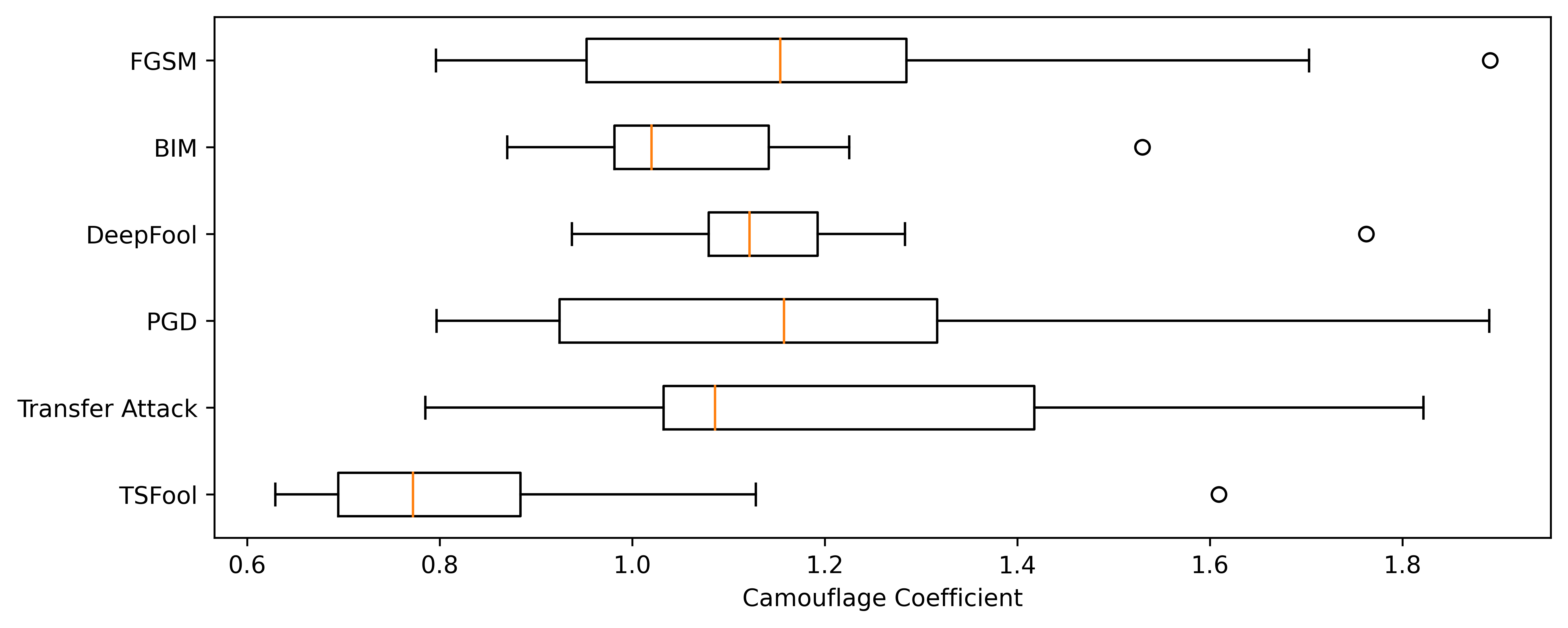
Figure 7: The distribution of Domain Perturbation Ratio $\rho^{*}$ and Camouflage Coefficient $\mathcal{C}$ of the experimental methods on the 10 UCR datasets.

VI Conclusion

In this paper, we propose the black-box TSFool attack to efficiently craft adversarial time series for RNN classifiers, significantly outperforming existing methods in effectiveness and imperceptibility. Although part of the reason for this result is the specificity of the RNN model and time series data mentioned, it also reflects the fact that the general consideration beyond image data and the feed-forward models is still lacking in the existing knowledge. For adversarial attack technology which is dedicated to opening a way toward the more robust and trustworthy model instead of just fooling some specific applications, such theoretical incompleteness would be a serious problem. This paper aims to introduce this situation to the community, and contribute some ideas for dealing with it.

The main contributions of this paper are as follows. Firstly, we propose a novel global optimization objective named Camouflage Coefficient to refine the adversarial attack as a multi-objective optimization problem, which may be instructive for crafting more imperceptible perturbation. Secondly, for the first time, we introduce the concept of the latent manifold to explain and directly guide the adversarial attack. Specifically, we build the representation model to capture potentially vulnerable samples having otherness between features and latent manifold. In this way, we can not only reduce the number of candidate target samples, but also heuristically approximate the optimal perturbation direction, so as to improve the efficiency and imperceptibility of adversarial attacks. Notice that our ideas can also be easily transferred to other types of models and data, which are expected to provide a new feasible way for the community to craft highly-imperceptible adversarial samples.

For future works, further exploring the newly defined multi-objective optimization problem to find better approximation solutions is an interesting topic, and the attempts to realize our idea in other kinds of adversarial attacks are in progress at present.

References

- [1] C. Szegedy, W. Zaremba, I. Sutskever, J. Bruna, D. Erhan, I. Goodfellow, and R. Fergus, “Intriguing properties of neural networks,” arXiv preprint arXiv:1312.6199, 2013.
- [2] X. Huang, D. Kroening, W. Ruan, J. Sharp, Y. Sun, E. Thamo, M. Wu, and X. Yi, “A survey of safety and trustworthiness of deep neural networks: Verification, testing, adversarial attack and defence, and interpretability,” Computer Science Review, vol. 37, p. 100270, 2020.
- [3] I. J. Goodfellow, J. Shlens, and C. Szegedy, “Explaining and harnessing adversarial examples,” arXiv preprint arXiv:1412.6572, 2014.
- [4] S.-M. Moosavi-Dezfooli, A. Fawzi, and P. Frossard, “Deepfool: a simple and accurate method to fool deep neural networks,” in Proceedings of the IEEE conference on computer vision and pattern recognition, 2016, pp. 2574–2582.
- [5] A. Kurakin, I. J. Goodfellow, and S. Bengio, “Adversarial examples in the physical world,” in Artificial intelligence safety and security. Chapman and Hall/CRC, 2018, pp. 99–112.
- [6] A. Madry, A. Makelov, L. Schmidt, D. Tsipras, and A. Vladu, “Towards deep learning models resistant to adversarial attacks,” arXiv preprint arXiv:1706.06083, 2017.
- [7] N. Papernot, P. McDaniel, A. Swami, and R. Harang, “Crafting adversarial input sequences for recurrent neural networks,” in MILCOM 2016-2016 IEEE Military Communications Conference. IEEE, 2016, pp. 49–54.
- [8] H. I. Fawaz, G. Forestier, J. Weber, L. Idoumghar, and P.-A. Muller, “Adversarial attacks on deep neural networks for time series classification,” in 2019 International Joint Conference on Neural Networks (IJCNN). IEEE, 2019, pp. 1–8.
- [9] T. Wu, X. Wang, S. Qiao, X. Xian, Y. Liu, and L. Zhang, “Small perturbations are enough: Adversarial attacks on time series prediction,” Information Sciences, vol. 587, pp. 794–812, 2022.
- [10] Y. Li, M. Cheng, C.-J. Hsieh, and T. C. Lee, “A review of adversarial attack and defense for classification methods,” The American Statistician, pp. 1–17, 2022.
- [11] A. Athalye, N. Carlini, and D. Wagner, “Obfuscated gradients give a false sense of security: Circumventing defenses to adversarial examples,” in International conference on machine learning. PMLR, 2018, pp. 274–283.
- [12] C. Fefferman, S. Mitter, and H. Narayanan, “Testing the manifold hypothesis,” Journal of the American Mathematical Society, vol. 29, no. 4, pp. 983–1049, 2016.
- [13] F. Chollet, Deep learning with Python. Simon and Schuster, 2021.
- [14] X. Zhang, X. Du, X. Xie, L. Ma, Y. Liu, and M. Sun, “Decision-guided weighted automata extraction from recurrent neural networks.” in AAAI, 2021, pp. 11 699–11 707.
- [15] H. A. Dau, A. Bagnall, K. Kamgar, C.-C. M. Yeh, Y. Zhu, S. Gharghabi, C. A. Ratanamahatana, and E. Keogh, “The ucr time series archive,” IEEE/CAA Journal of Automatica Sinica, vol. 6, no. 6, pp. 1293–1305, 2019.
- [16] H. Kim, “Torchattacks: A pytorch repository for adversarial attacks,” arXiv preprint arXiv:2010.01950, 2020.