The effects of surface fossil magnetic fields on massive star evolution: IV. Grids of models at Solar, LMC, and SMC metallicities

Abstract

Magnetic fields can drastically change predictions of evolutionary models of massive stars via mass-loss quenching, magnetic braking, and efficient angular momentum transport, which we aim to quantify in this work. We use the mesa software instrument to compute an extensive main-sequence grid of stellar structure and evolution models, as well as isochrones, accounting for the effects attributed to a surface fossil magnetic field. The grid is densely populated in initial mass (3-60 M_⊙), surface equatorial magnetic field strength (0-50 kG), and metallicity (representative of the Solar neighbourhood and the Magellanic Clouds). We use two magnetic braking and two chemical mixing schemes and compare the model predictions for slowly-rotating, nitrogen-enriched ("Group 2") stars with observations in the Large Magellanic Cloud. We quantify a range of initial field strengths that allow for producing Group 2 stars and find that typical values (up to a few kG) lead to solutions. Between the subgrids, we find notable departures in surface abundances and evolutionary paths. In our magnetic models, chemical mixing is always less efficient compared to non-magnetic models due to the rapid spin-down. We identify that quasi-chemically homogeneous main sequence evolution by efficient mixing could be prevented by fossil magnetic fields. We recommend comparing this grid of evolutionary models with spectropolarimetric and spectroscopic observations with the goals of i) revisiting the derived stellar parameters of known magnetic stars, and ii) observationally constraining the uncertain magnetic braking and chemical mixing schemes.

1 Introduction

Magnetism is ubiquitously present in the Universe, from the scale of sub-atomic particles up to the scale of galaxy clusters (e.g., Neronov & Vovk, 2010). For example, magnetic fields play a vital role in regulating star formation as molecular clouds collapse (e.g., Commerçon et al., 2011; Mackey & Lim, 2011; Crutcher, 2012; Hennebelle, 2013; Körtgen & Soler, 2020; Seifried et al., 2020), and in the formation and physics of neutron stars (e.g., Reisenegger, 2009; Beloborodov, 2009; Takiwaki et al., 2009; Takiwaki & Kotake, 2011; Mösta et al., 2015; Kuroda et al., 2020; Aloy & Obergaulinger, 2021; Reboul-Salze et al., 2021; Masada et al., 2022). In the phase between star formation and stellar end products, massive star evolution remains uncertain in part due to the incomplete understanding of stellar magnetic fields.

Spectropolarimetric surveys revealed that a subset (about 10%) of hot ($\gtrsim$ 10 kK), massive (8 - 60 M_⊙) and intermediate-mass (2 - 8 M_⊙) stars in the Galaxy with spectral types O, B, and A host large-scale, globally-organised surface magnetic fields (Morel et al., 2015; Fossati et al., 2016; Wade et al., 2016; Alecian et al., 2016; Grunhut et al., 2017; Shultz et al., 2018; Sikora et al., 2019a; Petit et al., 2019). Surface magnetic fields are detected both in chemically peculiar Bp/Ap stars, as well as in O, B, and A stars without observed chemical peculiarities (e.g., Donati & Landstreet, 2009; Henrichs et al., 2013; Neiner et al., 2015; Grunhut et al., 2017; Shultz et al., 2018; Sikora et al., 2019a). In addition, all known Of?p stars (showing variable emission in the Ciii$~{}\lambda$4647-4650-4652 complex, of comparable strength at its maximum to emission in the Niii$~{}\lambda$4634-4640-4642 complex, Walborn 1972) in the Galaxy are observed to be magnetic. Alongside spectropolarimetric observations, several properties may be used to identify magnetic candidates from photometric and spectroscopic studies, including multi-wavelength diagnostics (e.g., Babel & Montmerle, 1997; Cohen et al., 2003; Marcolino et al., 2012; Rivinius et al., 2013; Nazé et al., 2014; Oksala et al., 2015; Buysschaert et al., 2018; Walborn et al., 2015; Leto et al., 2021). Most recently, TESS photometric data is being used to identify candidate magnetic stars based on characteristic light-curve variations and subsequently observe them via spectropolarimetry (David-Uraz et al., 2019; Sikora et al., 2019b; Shultz et al., 2019c; David-Uraz et al., 2021b; Shultz et al., 2021a).

The observed surface magnetic fields of hot, massive and intermediate-mass stars do not show any apparent correlation with stellar and rotational parameters unlike in lower-mass ($<$2 M_⊙), cool stars ($<$10 kK), where magnetism due to surface convection and differential rotation ubiquitously produce dynamo activity (Donati & Landstreet, 2009; Neiner et al., 2015). Consequently, the organised, large-scale magnetic fields of hot stars are expected to be of fossil origin (Cowling, 1945; Spitzer, 1958; Mestel, 1967, 2003; Moss, 2003; Mestel & Moss, 2010; Ferrario et al., 2015; Braithwaite & Spruit, 2004, 2017). The exact origin of observed magnetic fields remains debated. In about 10% of intermediate-mass Herbig Be/Ae stars (which 10% is thought to be the precursors of main sequence Bp/Ap stars), large-scale surface magnetic fields are already observed on the pre-main sequence (Stȩpień, 2000; Alecian et al., 2009, 2013; Villebrun et al., 2019; Lavail et al., 2020), which may be acquired from the star-forming disk or generated via a dynamo action inside the star during a fully convective pre-main sequence phase (e.g. Moss, 2003; Braithwaite, 2012). In addition to magnetic fields possibly remaining from the star formation or pre-main sequence phases, stellar mergers could also amplify seed magnetic fields to a strength sufficient to be detectable (Ferrario et al., 2009; Wickramasinghe et al., 2014; Schneider et al., 2016; Schneider et al., 2019; Schneider et al., 2020), suggesting that there may exist multiple channels to generate globally-organised, large-scale fossil magnetic fields. Merger events of compact remnants have also been proposed to explain strongly magnetised white dwarfs and neutron stars (e.g., Tout et al., 2008; Giacomazzo et al., 2015; Ferrario et al., 2020; Caiazzo et al., 2021; Shultz et al., 2021b).

The nature of fossil fields is fundamentally different from contemporaneously generated dynamo fields by a mechanical source (such as convection or differential rotation). Fossil field evolution is purely dissipative with no active field generation counteracting its slow dissipation (Braithwaite & Spruit, 2017). In stellar layers where large-scale fossil fields spread through, it is expected that solid-body rotation will develop (e.g. Mestel, 1999). In those stellar layers the mechanical source of differential rotation is absent, and consequently small-scale dynamo fields in radiative stellar layers cannot be induced (Spruit, 2004). The Tayler instability (Tayler, 1973; Goldstein et al., 2019), for example, cannot develop if the radial rotation profile is completely flat, which means that the Tayler-Spruit (or "$\Omega$-type") dynamo cannot be induced in the presence of a fossil field (e.g., Spruit, 2004). In fact, while this type of dynamo mechanism in radiative stellar layers was proposed by Spruit (2002), there remains ongoing debate about the necessary electromotive force to operate the dynamo cycle (Fuller et al., 2019). The simulations of Zahn et al. (2007) suggest that this dynamo cycle does not operate. Despite the contradictory numerical results and the lack of direct observational evidence, dynamos in radiative stellar layers are commonly accounted for in evolutionary models (e.g., Spruit, 2002; Maeder & Meynet, 2003, 2004, 2005; Maeder, 2009; Heger et al., 2005; Yoon et al., 2006; Denissenkov & Pinsonneault, 2007; Potter et al., 2012b; Quentin & Tout, 2018; Fuller et al., 2019; Fuller & Ma, 2019; Takahashi & Langer, 2021). We emphasise that these implementations are not suitable (at least directly) to model stars that are known to host fossil fields.

The time evolution of fossil magnetic fields also remains an unresolved problem. Observed samples of magnetic A-type stars and compact remnants are consistent with the magnetic flux being conserved over time (e.g., Landstreet et al., 2007, 2008; Wickramasinghe & Ferrario, 2005; Neiner et al., 2017; Martin et al., 2018; Sikora et al., 2019a), whereas other observational evidence (including that for OB stars) suggests magnetic flux decay (e.g., Fossati et al., 2016; Shultz et al., 2019b). Fossil magnetic fields are expected to evolve only by Ohmic dissipation (Wright, 1969; Spruit, 2004; Duez & Mathis, 2010; Braithwaite & Spruit, 2017), which has a longer timescale than the main sequence nuclear timescale (Cowling, 1945; Spitzer, 1958). However, Ohmic dissipation remains riddled with uncertainties depending on the exact value of magnetic diffusivity (e.g., Charbonneau & MacGregor, 2001) and the geometry of the magnetic field since more complex fields dissipate faster.

Despite the uncertainties regarding the origin and evolution of fossil magnetic fields, it is now well established that they lead to various changes in stellar structure and evolution (e.g., Mestel, 1989, 1999; Duez & Mathis, 2010; MacDonald & Petit, 2019; Jermyn & Cantiello, 2020). Two main surface effects, mass-loss quenching and magnetic braking (discussed in detail below), have been shown to drastically modify evolutionary model predictions (e.g., Meynet et al., 2011; Keszthelyi et al., 2017a; Keszthelyi et al., 2019; Keszthelyi et al., 2020; Keszthelyi et al., 2021). For instance, heavy stellar-mass black holes and pair-instability supernovae could be formed from magnetic progenitors even at solar metallicity (Petit et al., 2017; Georgy et al., 2017).

Thus far, surface magnetic fields have only been detected in Galactic stars. Currently, high-resolution spectropolarimeters used for stellar magnetometry are employed on 4m-class telescopes, which limits observations to bright nearby stars. Using low-resolution spectropolarimetry, Bagnulo et al. (2017, 2020) searched for strong magnetic fields in the Magellanic Clouds through the Zeeman effect, which did not lead to definite detections in any of the targets. While high-resolution spectropolarimetry remains largely limited to a Galactic environment, very extensive spectroscopic campaigns in the Magellanic Clouds – in addition to the identified Of?p stars (e.g., Walborn et al., 2015; Munoz et al., 2020) – suggest that the nature of some stars may be explained by invoking surface magnetic fields (Hunter et al., 2008; Brott et al., 2011a; Rivero González et al., 2012; Potter et al., 2012b; Grin et al., 2017; Dufton et al., 2018; Dufton et al., 2020; Ramachandran et al., 2021). Observations of known magnetic stars in the Galaxy are often compared to evolutionary models that do not include fossil field effects (e.g., those of Brott et al. 2011a; Ekström et al. 2012; Chieffi & Limongi 2013; Choi et al. 2016; Costa et al. 2021; Grasha et al. 2021), possibly making inferences of stellar parameters rather uncertain. In turn, this can largely impact the derived ages of individual stars and bias isochrone fitting of stellar clusters. Therefore, there is a need for stellar evolution models (and model grids), which take into account mass-loss quenching and magnetic braking (although see Potter et al. 2012b for the latter), thereby affecting detailed evolutionary model predictions and population synthesis studies in both Galactic and extragalactic environments.

The motivation of this study is to help to resolve these issues by presenting and studying an extensive grid of stellar structure and evolution models with metallicities typical of environments in the Solar neighbourhood, Large Magellanic Cloud (LMC), and Small Magellanic Cloud (SMC) that include the effects of surface fossil magnetic fields. The model computations are open source and the entire library of models is available to the community via Zenodo at https://doi.org/10.5281/zenodo.7069766.

This paper is part of a series in which we aim to explore the effects of surface fossil magnetic fields on massive star evolution. In the first paper of the series (Keszthelyi et al., 2019, hereafter Paper I), we used the Geneva stellar evolution code (Eggenberger et al., 2008; Ekström et al., 2012; Georgy et al., 2013; Groh et al., 2019; Murphy et al., 2021) and discussed the mutual impact of magnetic mass-loss quenching, magnetic braking, and field evolution on a typical massive star of initially 15 M_⊙ at solar metallicity. We studied both solid-body and differentially-rotating models and evaluated their key evolutionary characteristics, showing that strong surface nitrogen enrichment is expected for magnetic models with differential rotation. In the second paper (Keszthelyi et al., 2020, hereafter Paper II), we elaborated on the implementation of massive star magnetic braking in the mesa software instrument (Paxton et al., 2011; Paxton et al., 2013, 2015, 2018, 2019) and detailed the magnetic and rotational evolution of the models by performing a parameter test in initial mass, magnetic field strength, and rotational velocity space with 35 models. Then, 72 tailored models were compared with a sample of observed magnetic B-type stars from Shultz et al. (2018); Shultz et al. (2019a); Shultz et al. (2019b). A key finding of Paper II is that magnetic stars could originate from ZAMS progenitors with a variety of parameter combinations. In Paper III (Keszthelyi et al. 2021) we focused on the scenario that some magnetic stars may originate from rapidly-rotating progenitors at the ZAMS, and specifically applied it to the case of the magnetic early B-type star $\tau$ Sco. We found that for this star the simultaneous nitrogen enrichment and slow rotation poses a significant challenge for single-star evolution.

The paper is organised as follows. In Section 2, we detail the assumptions and input physics used in the models. In Section 3, we present and scrutinise the stellar structure and evolution models from our computations. In Section 4, we discuss implications and future work. Finally, we conclude our findings in Section 5.

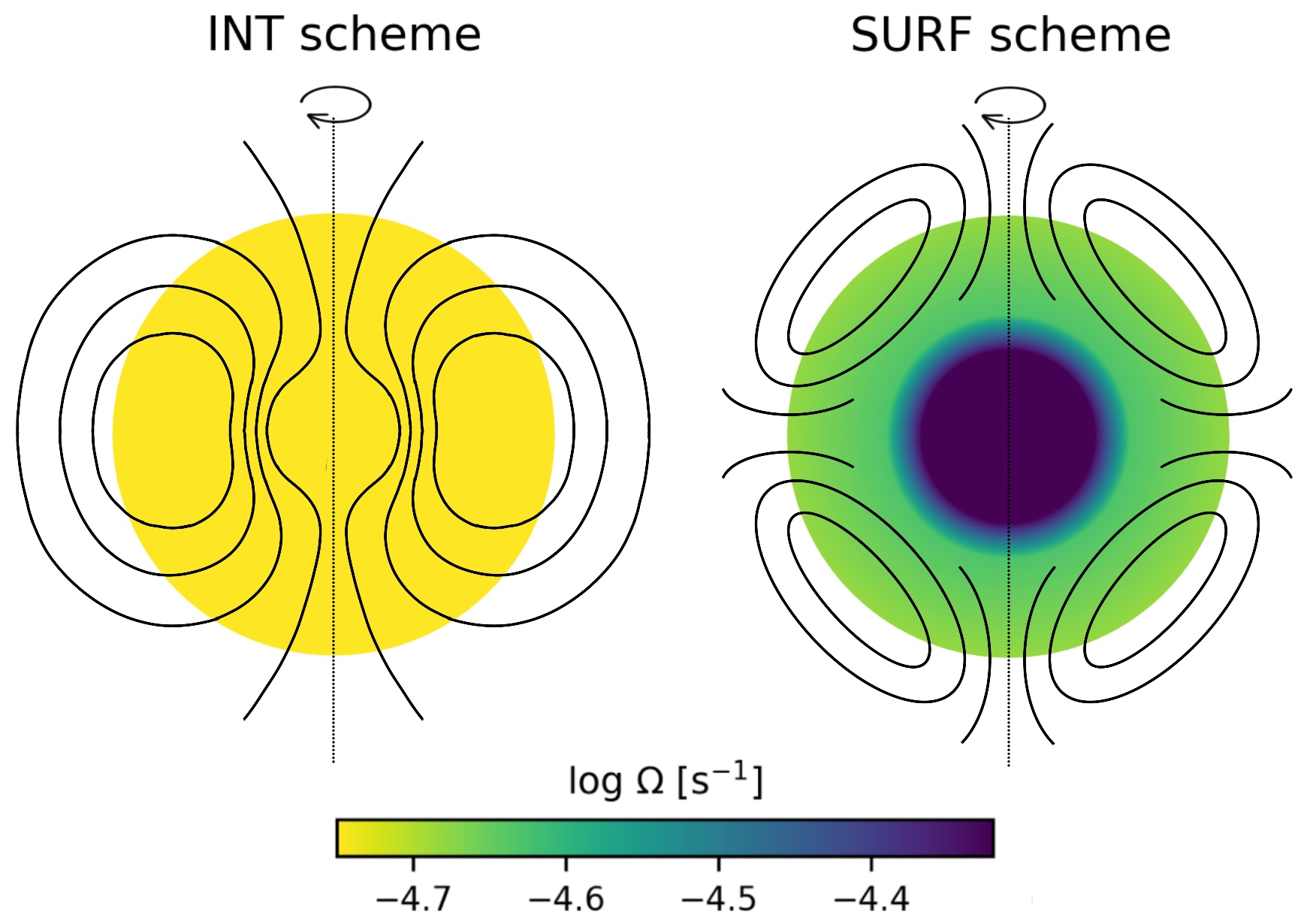
Figure 1: Schematic illustration of the magnetic field geometries (solid lines) considered in this study. These geometries are not directly implemented in our 1D models, instead they are used to constrain the corresponding scaling relations. Colours indicate the logarithmic angular velocity; the rotation axis is shown with dotted lines. Left: INT scheme, representative of a dipolar field configuration leading to internal magnetic braking, spinning down all layers of the star. As a phenomenological picture, we assume that convective expulsion (see Appendix C) would not allow the field to relax in the stellar core; however, we assume that the braking can propagate uniformly (including the core). The angular rotation is uniform throughout the star, enforced by a high diffusivity attributed to the dipole field. Right: SURF scheme, representative of a more complex field geometry leading to surface magnetic braking. The magnetic energy can be stored in higher-order spherical harmonics, and twisted field lines only penetrate to some extent of the envelope which we assume to be 20 per cent of the mass fraction. In those layers efficient angular momentum transport is present but we assume that core-envelope coupling is not achieved. Magnetic braking is only applied to those upper layers (see Section 2.6.1). To be able to incorporate the effects of such fields into 1D models, we assume that a quadrupole scaling may be used for calculating the Alfvén radius.

2 Modelling assumptions and setup

2.1 General strategy

In this work, we follow the general strategy of adopting suitable parametric prescriptions to model the effects of fossil magnetic fields, similar to the approaches presented in Paper I, Paper II, Paper III and references therein. While one-dimensional magnetohydrodynamic (MHD) approaches are possible, they have mostly been developed for dynamo models (e.g., Potter et al., 2012b; Feiden & Chaboyer, 2012, 2013; Quentin & Tout, 2018; Takahashi & Langer, 2021) and as such are not directly applicable to model fossil fields of intermediate-mass and massive stars. In particular, magnetic transport equations have been developed and used previously in the context of dynamo-generated fields (e.g., Spruit, 2002; Maeder & Meynet, 2003, 2004, 2005; Heger et al., 2005; Yoon et al., 2006; Potter et al., 2012b; Kissin & Thompson, 2018; Quentin & Tout, 2018; Fuller et al., 2019; Fuller & Ma, 2019; Takahashi & Langer, 2021). Although the characteristics (for example, the scale and time evolution) of dynamo models are incompatible with those of fossil fields (see Section 1), the transport equations may follow similar implementations. Here, we opt to artificially increase the diffusivity instead of testing "magnetic" transport equations (Section 2.6.2). Such equations would introduce more free parameters and further assumptions regarding the geometry, structure, and radial dependence of the magnetic field. Clearly, further research and observational verification is required before an appropriate one-dimensional magnetic transport process could be reliably incorporated to model stellar evolution with fossil magnetic fields (however, see Duez & Mathis 2010; Schneider et al. 2020). Duez & Mathis (2010) and Duez et al. (2010) presented a comprehensive approach applicable for fossil fields, showing however that the impact on hydrodynamic equilibrium and energy transport are modest even for strong magnetic fields. To this extent, it is indeed appropriate to use parametric prescriptions and focus on the major, measurable effects that fossil magnetic fields have, namely changing the mass loss (Section 2.5) and rotation (Section 2.6) of the star, affecting chemical mixing and angular momentum transport.

One of the major modelling challenges is that the geometry and alignment of the magnetic field play a significant role in the corresponding physical description. It has been demonstrated that a seed magnetic field can relax into a stable axisymmetric (around the magnetic axis) configuration if the magnetic flux is centrally concentrated, or into a non-axisymmetric (around the magnetic axis) configuration otherwise (Braithwaite & Spruit, 2004; Braithwaite & Nordlund, 2006; Braithwaite, 2008). In both cases, the latitudinal averaging is inappropriate to model the magnetic field in 1D.

For simplicity, we assume that the field is aligned with the rotation axis of the star since appropriate scaling relations for oblique fields (tilted with respect to the rotation axis) are still in development. However, the obliquity angles inferred from observations appear to follow a random distribution, which suggests that, apart from a few possible exceptions, massive stars generally possess magnetic fields that are inclined with respect to the rotation axis (e.g., Khalack et al., 2003; Shultz et al., 2019a; Sikora et al., 2019a). Recent work from ud-Doula (2020) suggests that oblique rotation leads to decreasing the efficiency of magnetic braking. This effect could be incorporated in our models via a suitable scaling factor in future studies. However, the efficiency of magnetic braking, in the evolutionary context, is also largely dependent on magnetic field evolution, which still needs to be better constrained (e.g., Paper III).

In fact, magnetic field evolution is closely tied to the question of the field geometry and, in this regard, new insights are gained from extensive monitoring campaigns, which can reveal the surface properties of magnetic fields. Although a purely dipolar field geometry generally matches observations (Grunhut et al., 2017; Shultz et al., 2018), modest deviations from pure dipolar geometries are now identified (Leto et al., 2018; Das et al., 2020; David-Uraz et al., 2021a). In other cases, contributions from higher-order harmonics are also identified (e.g., Shultz et al. 2018; Kochukhov et al. 2019); however, the dipole is the strongest component, which consequently drives the main physical effects. In a few cases, observations have also identified stars with uniquely complex magnetic fields, which cannot be described with a dominant dipole component (e.g., $\tau$ Sco, Donati et al., 2006; Kochukhov & Wade, 2016; Shultz et al., 2018). In these cases, most of the magnetic energy is stored in higher-order spherical harmonics, although a weak dipole contribution may still be present.

Since the structure of large-scale magnetic fields in stellar interiors is still considerably uncertain, we aim to test two limiting cases - illustrated in Figure 1 - to apply depth-dependent magnetic braking (c.f. Paper II). In the models with internal magnetic braking (INT, described in detail below), we assume that the magnetic field is dipolar. We further assume that the field is present in the entire stellar envelope and is able to achieve core-envelope coupling (however, only as a phenomenological picture, we assume that it is excluded from the stellar core). In nature, the stellar envelope must also have a closed toroidal field for a stable configuration (Wright, 1969, 1973; Braithwaite & Spruit, 2004; Braithwaite & Nordlund, 2006; Akgün et al., 2013), which we cannot directly take into account in our 1D models. The magnetic field is curl-free above the stellar surface; any toroidal field diffuses to a poloidal structure. We also introduce a set of models with surface magnetic braking (SURF, see also below) as a limiting scenario to contrast the INT models with. The complex magnetic field geometries clearly cannot be translated to our 1D models, therefore we make various simplifying assumptions (discussed in detail throughout Section 2). We reiterate that the field geometry cannot be directly included in our models, only via the scaling relations. The limitations related to the 1D parametrisation can likely only be resolved once 2D stellar evolution modelling becomes feasible (Espinosa Lara & Rieutord, 2011; Lovekin, 2020; Reese et al., 2021).

Angular momentum is always lost from the outermost layers of the star. We use the INT/SURF schemes to control the propagation of this loss to the stellar interiors along with efficient angular momentum transport. In the INT models, all stellar layers efficiently transport and lose specific angular momentum. Motivated by the simulations of Braithwaite (2008), we assume that in the SURF models the magnetic-field driven angular momentum transport and rotational braking only affect the upper 20% of stellar mass. Although even for complex surface magnetic fields there may be weak dipole contributions, we neglect here any possible magnetic angular momentum transport in the deep stellar interiors so that we are able to test a limiting case in which radial differential rotation may develop in regions of the star where the magnetic flux is assumed to be negligible. Furthermore, to generalise from the range of possible field configurations deduced from observations, we assume that at least the Alfvén radius (see section 2.4) has to be smaller in the SURF models than in the INT models for a given surface field strength. For this reason, we use a quadrupole scaling in the SURF models to obtain the Alfvén radius. This results in less efficient magnetic braking for complex fields compared to dipole-dominated geometries. The field geometry defines the wind flow and mass flux from the stellar surface. We evaluate in Appendix B how an actual quadrupole field geometry would affect mass-loss quenching; however, since this effect only concerns the highest-mass models, for simplicity we adopt a formalism where only the Alfvén radius is changed in the SURF models compared to the INT models (see Section 2.5).

2.2 General model setup

We use the software instrument Modules for Experiments in Stellar Astrophysics mesa release 15140 (Paxton et al., 2011; Paxton et al., 2013, 2015, 2018, 2019) and Software Development Kit (SDK) version 20.12.1 (Townsend, 2020), and carry out our computations on the Dutch supercomputers Cartesius and Snellius. In this study, we consider main sequence models with initial masses from 3 to 60 M_⊙ (Table 1). This choice is made since there are still considerable uncertainties in stellar evolution, as well as in magnetic field evolution on the post-main sequence. The computations begin by relaxing the initial model and we consider the Zero Age Main Sequence (ZAMS) to begin at the time when the initial abundance of core hydrogen has decreased by 0.3 percent. The endpoint of the models is the Terminal Age Main Sequence (TAMS), which we consider at the time when the core hydrogen mass fraction drops below $10^{-5}$.

The mesa microphysics are summarised in Appendix A. To calculate the nuclear reaction rates, we use mesa’s default "basic.net" option. To model convective mixing, we assume a mixing length parameter of $\alpha_{\rm MLT}=1.8$ (e.g., Canuto & Mazzitelli, 1992; Canuto et al., 1996) and the Henyey formalism (Henyey et al., 1965) in mesa. Common values of $\alpha_{\rm MLT}$ range from 1.5 to 2.0, mostly based on solar and solar-type star calibrations (e.g., Bonaca et al., 2012). For simplicity, we assume the same value in all models, although some studies predict mass dependence (e.g., Yıldız et al., 2006). Semiconvective and thermohaline mixing are not used. Convective boundaries are determined via the Ledoux criterion. Core overshooting is applied in the exponential scheme with parameters $f_{\rm ov}=0.015$ and $f_{0}=0.005$, which roughly corresponds to a step overshoot parameter $\alpha_{\rm ov}$ of 10 percent of the local pressure scale height (Ekström et al., 2012, see further discussion in Appendix C). $\alpha_{\rm ov}$ may be mass dependent (Castro et al., 2014). Commonly used values of $\alpha_{\rm ov}$ range from 0.1 to 0.335, (Schaller et al., 1992; Brott et al., 2011a). Exponential overshooting at non-burning convective regions is adopted with $f_{\rm ov}=0.0010$ and $f_{0}=0.0005$. mesa’s MLT++ scheme is not applied (see e.g., Poniatowski et al. 2021).

We employ high spatial and temporal resolution by setting mesh_delta_coeff = 1. and time_delta_coeff = 1., in addition to setting varcontrol_target = 1.d-4. This results in an average of 2000-3000 zones for our stellar structure models, and the evolutionary models consist of a hundred to a few thousand structure models (each corresponding to one time step), mostly depending on the initial mass.

We consider one initial rotation rate in all models by relaxing an initial ratio of $\Omega/\Omega_{\rm crit}=0.5$. In our models with solar metallicity, this approximately corresponds to an initial equatorial surface rotational velocity (surf_avg_vrot in mesa) of 300 to 370 km s^-1 in the initial stellar mass range from 3 to 60 M_⊙. The critical angular velocity is adopted as defined in mesa star_utils.f90:

$$\Omega_{\rm crit}=\sqrt{(1-\Gamma)\frac{Gm}{r^{3}}}\,,$$ (1)

where the Eddington parameter is $\Gamma=L_{\rm rad}/L_{\rm Edd}$, G is the gravitational constant, and $m$ and $r$ are the mass and radius taken at the photosphere. This definition only plays a role in setting the initial rotational velocity. The initial model relaxes from solid-body rotation to a new configuration constrained by angular momentum distribution and transport.

In Paper II we found that a lower rotation rate (initially $\Omega/\Omega_{\rm crit}=0.2$) leads to smaller differences between models with and without magnetic fields. This is simply because magnetic braking is less efficient when the rotation is slow. In Paper II, we showed that at least a few magnetic stars were best matched with models that had an initial rotation rate of $\Omega/\Omega_{\rm crit}=0.8$. If the initial rotation rate was higher than considered in this study, it would i) alter the early evolution of the models on the Hertzsprung-Russell diagram (HRD, as shown in Figure 3 of Paper II), and ii) impact the quantitative predictions regarding the surface chemical enrichment. It is worth noting that the most rapidly rotating (presumably young) magnetic stars have present-day surface rotational velocities of about 300 km s^-1, which is close to 50% of the critical rotation defined in our Equation 1 (e.g., Oksala et al., 2010; Grunhut et al., 2012; Shultz et al., 2019b; Song et al., 2021). Nevertheless it remains unknown what initial rotation rates could characterise the entire sample of magnetic massive stars.

Finally, given the supporting observational evidence by some studies (Kochukhov & Bagnulo, 2006; Wickramasinghe & Ferrario, 2005; Neiner et al., 2017; Martin et al., 2018; Sikora et al., 2019a), we assume magnetic flux conservation (Alfvén’s theorem, Alfvén 1942) such that the surface magnetic field strength is obtained from:

$$B_{\rm eq}=B_{\rm eq,ini}\left(\frac{R_{\rm\star,ini}}{R_{\star}}\right)^{2}$$ (2)

with $B_{\rm eq,ini}$ being the initial surface equatorial magnetic field strength (which is assumed in the models at the ZAMS), while $R_{\rm\star,ini}$ and $R_{\star}$ are the initial and current stellar radii. For further discussions on magnetic field evolution, we refer the reader to Paper I, Paper II, Paper III and references therein. We adopt a large range of initial equatorial magnetic field strengths (from 0 to 50 kG; Donati & Landstreet 2009, e.g.,; Shultz et al. 2019b, e.g.,.)

The run_star_extras file (available as part of a full reproduction package on Zenodo at https://doi.org/10.5281/zenodo.7069766) is used to modify the wind, torque, angular momentum transport, and chemical element transport routines. The parameters varied in the models are summarised in Tables 1, 2, and 3, and are discussed below.

Table 1: Comprehensive grid of 8,748 mesa evolutionary models including the effects of surface fossil magnetic fields, covering a large parameter space in initial mass and magnetic field strength (see below) for 3 metallicities (Table 2) and for 2 braking schemes and 2 mixing schemes (Table 3).

$M_{\rm\star,ini}$ [M⊙]	3, 4, 5, 6, 7, 8, 9, 10, 11, 12, 13, 14, 15, 16, 17, 18, 19, 20, 21, 22, 23, 24, 25, 30, 40, 50, 60
$B_{\rm eq,ini}$ [kG]	0, 0.25, 0.50, 0.75, 1.0, 1.5, 2.0, 2.5, 3.0, 3.5, 4.0, 4.5, 5.0, 5.5, 6.0, 6.5, 7.0, 7.5, 8.0, 8.5, 9.0, 9.5, 10, 15, 20, 30, 50

Table 2: Key initial elemental abundances (in mass fractions and compared to the adopted solar value) included in our models.

	Xini	$\frac{\mathrm{X_{ini}}}{\mathrm{X_{\odot,ini}}}$	Yini	$\frac{\mathrm{Y_{ini}}}{\mathrm{Y_{\odot,ini}}}$	Zini	$\frac{\mathrm{Z_{ini}}}{\mathrm{Z_{\odot,ini}}}$	Cini	$\frac{\mathrm{C_{ini}}}{\mathrm{C_{\odot,ini}}}$	Nini	$\frac{\mathrm{N_{ini}}}{\mathrm{N_{\odot,ini}}}$	Oini	$\frac{\mathrm{O_{ini}}}{\mathrm{O_{\odot,ini}}}$
Solar	0.72000	1	0.26600	1	1.40000 $\cdot$10-2	1	1.84720 $\cdot$10-3	1	6.21528 $\cdot$10-4	1	6.62907 $\cdot$10-3	1
LMC	0.73685	1.02	0.25671	0.97	6.43605 $\cdot$10-3	0.46	9.25898 $\cdot$10-4	0.50	1.45717 $\cdot$10-4	0.24	2.96143 $\cdot$10-3	0.45
SMC	0.74840	1.04	0.24900	0.94	2.60758 $\cdot$10-3	0.19	2.15433 $\cdot$10-4	0.12	6.76488 $\cdot$10-5	0.11	1.34354 $\cdot$10-3	0.20

2.3 Metallicity

We compute models for 3 different metallicities (the key elements are summarised in Table 2 – the full list of abundances is available via the model files shared on Zenodo) that are representative of the Solar neighbourhood, LMC, and SMC. For the Solar composition, we assume the hydrogen and helium mass fractions along with a metallicity of $Z=0.014$ (Asplund et al., 2009). The metal fractions are adopted following the works of Przybilla et al. (2008); Przybilla et al. (2013) and Nieva & Przybilla (2012), which updated some elements compared to the Asplund et al. (2005); Asplund et al. (2009) abundances, considering B-type stars in the solar neighbourhood. The baseline values for the Magellanic Clouds are still subject to ongoing investigations (e.g., Dufton et al., 2020; Bouret et al., 2021). For the helium and metal abundances in the LMC and SMC, we adopt the mean values listed in Tables 5 and 6 of Dopita et al. (2019). These mean values are a result of 9 separate investigations using different approaches, which include atmospheric determinations of hot stars, supernova remnants, and H  ii regions. In all 3 metallicities, we use the Lodders (2003) isotopic ratios. The metallicity adopted for the chemical composition is fully consistent with the metallicity used for the opacity tables.

2.4 Alfvén radius

The Alfvén radius characterises a critical distance at which the magnetic energy density and the gas kinetic energy density are equal. Alternatively, it can also be cast as the inverse square of the Alfvénic Mach number. Its definition plays an important role in both mass-loss quenching (Equations 7-8) and magnetic braking (Equations 9-10). For a dipolar field configuration, ud-Doula et al. (2009) use a numerical fitting for a quartic equation to obtain:

$$\frac{R_{\rm A}}{R_{\star}}\approx 1+(\eta_{\star}+0.25)^{1/4}-(0.25)^{1/4}\,,$$ (3)

with $\eta_{\star}$ the equatorial magnetic confinement parameter, defined as:

$$\eta_{\star}=\frac{B_{\rm eq}^{2}R_{\star}^{2}}{\dot{M}_{B=0}v_{\infty}}\,,$$ (4)

with $B_{\rm eq}$ the equatorial magnetic field strength, $\dot{M}_{B=0}$ the mass-loss rate in absence of a magnetic field, and $v_{\infty}$ the terminal velocity (ud-Doula et al., 2009). Observations typically reconstruct a polar field strength $B_{\rm p}$ from the line-of-sight disc-integrated (so called longitudinal) magnetic field strength (Donati & Landstreet, 2009). The equatorial field strength is exactly one half of the polar field strength. We use Equation 3 to obtain the Alfvén radius in the INT models, which we assume to be characterised by a predominantly dipolar field configuration (Figure 1). In the SURF models we assume the field to be more complex, in which case the definition of the Alfvén radius is non trivial. For the sake of simplicity we assume that the Alfvén radius takes the form of a scaling appropriate for a quadrupole field geometry, such that:

$$\frac{R_{\rm A}}{R_{\star}}\approx 1+(\eta_{\star}+0.25)^{1/6}-(0.25)^{1/6}\,,$$ (5)

following the parametrisation in Equation 9 of ud-Doula et al. (2008). This ensures that for a given field strength $R_{\rm A}$ is less in the SURF case than in the INT case, leading to less efficient magnetic braking.

2.5 Stellar winds

2.5.1 Mass-loss schemes and terminal velocities

The models include mass loss. Even though this is modest for the lower-mass stars (and the driving mechanism is not unambiguously identified as for more massive stars), it can impact their rotational evolution given the longer nuclear timescale. For this reason, we apply commonly used mass-loss rates of hot massive stars also to lower mass main sequence stars in our grid. While the higher-mass stars typically reach the TAMS at $T_{\rm eff}>20$ kK, we describe here the detailed treatment implemented in our mesa extension for completeness and to aid further studies focusing on complementing this work with post-main sequence models. For massive stars with $T_{\rm eff}>10$ kK, the mass loss is powered by radiative line driving (e.g., Lucy & Solomon, 1970; Castor et al., 1975; Puls et al., 2008). In this regime, we apply the rates derived by Vink et al. (2000, 2001), decreased by a factor of 2 for all models in the 3 - 60 M_⊙ range for consistency. The choice to reduce the nominal mass-loss rates is motivated by the growing evidence both from observations, suggesting that mass-loss rates are lower when accounting for wind clumping (e.g., Bouret et al., 2005; Fullerton et al., 2006; Trundle & Lennon, 2005; de Almeida et al., 2019; Brands et al., 2022), and from new modelling approaches (e.g., Muijres et al., 2012; Krtička, 2014; Krtička & Kubát, 2017; Krtička et al., 2021; Sundqvist et al., 2019; Björklund et al., 2021). When using these rates, we apply metallicity-dependent winds with a scaling of $\dot{M}\sim Z^{0.85}$ (e.g., Vink et al., 2001; Mokiem et al., 2007).

Similarly to Keszthelyi et al. (2017b) and Paper II, we implement the partitioning in effective temperature related to the bi-stability jump at 20 kK in agreement with observational and new theoretical works (Prinja et al., 1990; Prinja & Massa, 1998; Lamers et al., 1995; Petrov et al., 2016), rather than adopting it at 25-27 kK as in evolutionary models of e.g., Brott et al. (2011a), Ekström et al. (2012), and Choi et al. (2016). This is further supported by measurements of projected rotational velocities that suggest a lack of bi-stability braking (Crowther et al., 2006; Vink et al., 2010; Keszthelyi et al., 2017b; Gagnier et al., 2019a, b; Krtička et al., 2021; Vink & Sander, 2021) at least until about 20 kK (Howarth et al., 1997; Huang et al., 2010). Although we adopt an increase in mass-loss rates at the bi-stability jump, we note that this prediction still lacks empirical evidence in typical B-type supergiants (Crowther et al., 2006; Markova & Puls, 2008; Rubio-Díez et al., 2022) and is challenged by new numerical simulations (Sundqvist et al., 2019; Driessen et al., 2019b; Björklund et al., 2021).

Below approximately 10 kK the nature of wind-driving remains poorly understood. We opt to use the rates of van Loon et al. (2005) for all models in this domain, which only concerns a few lower-mass models in the present grid. New modelling approaches have confirmed that the second bi-stability jump due to Fe iii recombining to Fe ii is expected at $T_{\rm eff}\sim$ 9 kK (Petrov et al., 2016) in contrast with earlier indications of $\sim$ 12.5 kK (Vink et al., 1999, 2000), and implementations in evolutionary models of $\sim$ 17-15 kK (Ekström et al., 2012; Brott et al., 2011a). Therefore we avoid the use of the second bi-stability jump that is typically included in other grids of models (for further details see, e.g., Figure 3 of Keszthelyi et al. 2017b). If the effective temperature is higher than 10 kK and the surface hydrogen mass fraction becomes less than 0.4, we apply the Wolf-Rayet rates of Nugis & Lamers (2002). This concerns some of our most massive models with efficient mixing.

In agreement with the partitionings in effective temperature, we estimate the terminal wind velocity $v_{\infty}$ via:

$$v_{\infty}=f_{\infty}\cdot\,v_{\rm esc}=f_{\infty}\,\sqrt{\frac{2GM_{\star}}{R_{\star}}\left(1-\Gamma_{e}\right)}\,,$$ (6)

where $G$, $M_{\star}$, $R_{\star}$, and $\Gamma_{e}$ are respectively the gravitational constant, the stellar mass, the stellar radius, and the Eddington parameter for pure electron scattering. The terminal wind velocity is obtained from the escape velocity as a simple step function by adopting $f_{\infty}=2.6,1.3,0.7$ at $T_{\rm eff}>20$ kK, $20\,\mathrm{kK}>T_{\rm eff}>10$ kK, and $T_{\rm eff}<10$ kK, respectively (Lamers et al., 1995; Vink et al., 2000; Kudritzki & Puls, 2000). The typical terminal velocities at the ZAMS range from 800 to 3000 km s^-1 for models with initial masses from 3 to 60 M_⊙, respectively. We calculate the rotational enhancement on the mass-loss rates as described by Maeder & Meynet (2000). This requires defining the difference of the force multiplier parameters $\alpha^{\prime}$ ($=\alpha-\delta$, that is, the exponent related to the line-strength distribution function minus the exponent quantifying the change in ionisation balance), which we adopt as a simple step function with values of 0.6, 0.5, 0.4, corresponding to the above-mentioned effective temperature ranges (see Pauldrach et al., 1986; Lamers et al., 1995; Puls et al., 2000). The alternative calculation of rotational enhancement built into mesa is not used (see Paper II Section 3.9 for details).

2.5.2 Magnetic mass-loss quenching

The overall field configuration that extends into the wind outflow is governed by the competition between the kinetic energy of the wind and the magnetic energy of the field. The ionised stellar wind material is forced to flow along magnetic field lines. However, as the wind kinetic energy density has a shallower decline than the magnetic energy density, the field loops can only confine wind material up to a certain radius. Within closed field loops, material becomes trapped and eventually falls back onto the surface (unless centrifugally supported). To account for the global, time-averaged effect of the magnetosphere, the mass-loss rates are systematically reduced. Following the works of ud-Doula et al. (2008, 2009), the mass-loss quenching parameter $f_{\rm B}$ is defined as:

$$f_{\rm B}=\,\frac{\dot{M}}{\dot{M}_{B=0}}=\,1-\sqrt{1-\frac{1}{R_{\rm c}}}\quad\mathrm{if}\quad R_{\rm A}<R_{\rm K}$$ (7)

and

$$f_{\rm B}=\,\frac{\dot{M}}{\dot{M}_{B=0}}\,=2-\sqrt{1-\frac{1}{R_{\rm c}}}-\sqrt{1-\frac{0.5}{R_{\rm K}}}\quad\mathrm{if}\quad R_{\rm K}<R_{\rm A}$$ (8)

where $R_{\rm A}$, $R_{\rm K}$, and $R_{\rm c}$ are the Alfvén radius, the Kepler co-rotation radius, and the closure radius in units of the stellar radius, respectively (see Petit et al. 2017, Paper I, Paper II, Paper III, and references therein). The closure radius, defining the distance from the stellar surface to the last closed magnetic loop, is approximated as $R_{\rm c}~{}\sim~{}R_{\star}~{}+~{}0.7~{}(R_{\rm A}~{}-~{}R_{\star}~{})$, see ud-Doula et al. (2008). $\dot{M}$ is the mass-loss rate that a non-rotating magnetic star would have. $\dot{M}$ is further scaled by the rotational enhancement $f_{\rm rot}$ (specified in Section 3.9 of Paper II) such that the effective mass-loss rate is obtained from $\dot{M}_{\rm eff}=f_{\rm B}\cdot f_{\rm rot}\cdot\dot{M}_{B=0}$. The magnetic mass-loss quenching parameter (equivalent to the escaping wind fraction) can take values between 0 and 1, depending on the magnetic field strength. A strong magnetic field (with a strength of tens of kG) may lead to only a few percent of the wind material actually escaping the star (Petit et al. 2017; Georgy et al. 2017, Paper I). Let us also note that the conditions in the above equations are equivalent to distinguishing between dynamical magnetospheres (if $R_{\rm A}<R_{\rm K}$) and centrifugal magnetospheres (if $R_{\rm K}<R_{\rm A}$), a classification introduced by Petit et al. (2013).

The use of Equation 8 is a refinement compared to previous implementations. For situations when the Alfvén radius is larger than the Kepler co-rotation radius (centrifugal magnetospheres), the magnetosphere is expected to be less efficient at quenching wind mass-loss compared to dynamical magnetospheres (ud-Doula et al., 2008, 2009). This is because material injected by the wind into the centrifugal magnetosphere is not returned to the stellar surface by gravity, but is instead ejected away from the star once the critical centrifugal breakout density is exceeded (Shultz et al., 2020; Owocki et al., 2020). This can lead to substantially larger values of $f_{\rm B}$ for a rotating as compared to a non-rotating star, however in practice rapid spin-down means that centrifugal magnetospheres are relatively short-lived and the incorporation of this modification to the mass-quenching prescription does not have a strong effect on evolution. It is generally expected that the evolution proceeds from centrifugal to dynamical magnetospheres (Shultz et al. 2019b, Paper I, Paper II).

In this approach, the magnetic mass-loss quenching parameter is an average quantity. MHD simulations of non-rotating magnetospheres predict up- and down-flows of material varying on short dynamical timescales (ud-Doula & Owocki, 2002), which can manifest as stochastic variability in magnetospheric emission lines (ud-Doula et al., 2013), however time-averaged models provide a good reproduction of emission line properties (e.g. Sundqvist et al., 2012; Owocki et al., 2016; Erba et al., 2021) and these short-term, stochastic variations can therefore be confidently neglected over evolutionary timescales. In the case of rapid rotators, 2D MHD simulations led to the expectation that breakout events would be similarly stochastic, leading to emptying of the centrifugal magnetosphere and large-scale magnetospheric reorganisation (ud-Doula et al., 2006, 2008). However, no indication of large-scale changes has been observed (Townsend et al., 2013; Shultz et al., 2020), leading Shultz et al. (2020) and Owocki et al. (2020) to infer that breakout events are characterised by small spatial scales and occur more or less continuously, such that the centrifugal magnetosphere is maintained nearly continuously at the breakout density. As a result, it is therefore appropriate to treat magnetospheric mass-drainage via breakout as an effectively continuous process over evolutionary timescales and apply Equations 7 and 8.

Table 3: Magnetic braking and chemical mixing schemes

INT:	solid-body rotation, braking the rotation of the entire star
SURF:	differential rotation, braking the rotation of the surface
Mix1:	$D_{\rm chem}$ defined by Equation 16 with $f_{\rm c}=0.033,f_{\mu}=0.1$
Mix2:	$D_{\rm chem}$ defined by Equation 22 with $f_{\rm c}=1,f_{\mu}=1$

2.6 Angular momentum transport and loss

Magnetic fields are much more efficient at transporting angular momentum than purely hydrodynamic processes such as meridional currents and shear instabilities (e.g., Mestel, 1999; Spruit, 1999, 2002; Kulsrud, 2005; Braithwaite & Spruit, 2017). The rotation of the star leads to Maxwell stresses, which result in losing angular momentum from the star.

In Paper I, genec models were used, where magnetic braking is adopted as a boundary condition to internal angular momentum transport, directly affecting the uppermost layer of the stellar models. In Paper II, two kinds of models were introduced to account for the uncertainty regarding how deeply fossil magnetic fields are anchored in massive stars. In the INT models, magnetic braking was applied to the entire star, decreasing uniformly the specific angular momentum in all layers. In the SURF models, magnetic braking was set to remove specific angular momentum from a very near-surface reservoir. In Paper III, genec models were contrasted with a mesa implementation where magnetic braking was applied to most of the stellar envelope. In genec, two configurations were used to model internal angular momentum transport: one with only hydrodynamic instabilities correctly accounted for via an advecto-diffusive equation (allowing for shears to develop in deeper layers), and one with a purely diffusive equation, in which solid-body rotation was established. In mesa, we relied on the nominal hydrodynamic transport processes since they are used in a purely diffusive assumption, leading to nearly solid-body rotation on the magnetic braking timescale. Here, we make some further refinements and adjustments compared to these approaches, particularly accounting (indirectly) for the field geometry as depicted in Figure 1.

2.6.1 Magnetic braking

Stellar rotation bends and twists magnetic field lines in the azimuthal direction. Magnetic field lines can transport and store angular momentum, and the associated Maxwell stresses are very efficient at transferring angular momentum to the surrounding plasma. Once the angular momentum is imparted from the field to the gas, the wind material carries it away, leading to a spin-down of the star. This process is commonly referred to as (wind) magnetic braking.

In a pioneering series of works, analytical and numerical MHD simulations were developed, confirming that the Weber & Davis (1967) model (see also, Parker 1958; Mestel 1968) leads to an appropriate scaling relation also for massive stars (ud-Doula & Owocki, 2002; ud-Doula et al., 2008, 2009; Owocki & ud-Doula, 2004; Townsend & Owocki, 2005). Following the work of ud-Doula et al. (2009), the total – wind and magnetic field induced – loss of angular momentum can be expressed via:

$$\frac{\mathrm{d}J_{\rm B}}{\mathrm{d}t}=\frac{2}{3}\dot{M}_{B=0}\,\Omega_{\star}R_{A}^{2}\,,$$ (9)

with $\mathrm{d}J_{\rm B}/\mathrm{d}t$ the rate of angular momentum loss from the system, $\Omega_{\star}$ the surface angular velocity, and $R_{A}$ the Alfvén radius (defined in Equations 3 and 5). As this equation accounts for the gas and field driven angular momentum loss (ud-Doula et al., 2009), it yields the angular momentum loss resulting purely from mass loss when $B_{\rm surf}=0$. As specified in Paper II, we have adjusted the angular momentum lost via mass loss to avoid double counting. In Equation 9, the numerical term 2/3 arises from integrating over latitudes. We note that this equation is not applicable when the effective mass-loss rate, as introduced above, is exactly zero (this situation does not happen in our models). In the strong confinement limit, when $f_{\rm B}\rightarrow 0$, the effective mass-loss rate can become very small. In this case, a strong magnetic braking can still be achieved since the Maxwell stresses driving the angular momentum transport are independent of the plasma flow. As long as there is wind material at a radial distance larger than the last closed magnetic field line, i.e., the star is not surrounded by vacuum, the field can impart angular momentum to the plasma. In Paper II and Paper III, Equation 9 was implemented into mesa via changing the specific angular momentum in given layers of the star, such that a summation over mass yields the total rate of angular momentum loss as defined in Equation 9. It is coded as:

$$\frac{\mathrm{d}J_{\rm B}}{\mathrm{d}t}=\sum_{k=1}^{k=x}\frac{\mathrm{dj_{\rm B}}}{\mathrm{d}t}=-\frac{\mathrm{d}J_{\rm B}}{J_{\rm INT/SURF}}\sum_{k=1}^{k=x}\frac{\mathrm{d}j}{\mathrm{d}t}\,,$$ (10)

where $\mathrm{d}j_{\rm B}/\mathrm{d}t$ is the rate of specific angular momentum change (dubbed as "extra_jdot" in mesa). The negative sign is added to reduce the reservoir (i.e., to account for loss), $\mathrm{d}J_{\rm B}=(\mathrm{d}J_{\rm B}/\mathrm{d}t)\cdot\mathrm{d}t$ is the total angular momentum lost per time $\mathrm{d}t$, $J_{\rm INT/SURF}$ is the angular momentum reservoir of the entire star (INT) or of defined layers in the stellar envelope (SURF; see Figure 1 and discussion below), $j$ is the specific angular momentum of a layer (called "j_rot" in mesa), d$t$ is one timestep in the computation, $k$ is an index running through all layers, and $x$ is the index of the last layer where magnetic braking is applied. Therefore, Equation 10 indicates how to distribute the total angular momentum lost per unit time ($\mathrm{d}J_{\rm B}/\mathrm{d}t$ given by Equation 9) in given stellar layers. Taking the sum of the specific angular momentum lost per unit time $\mathrm{d}j_{\rm B}/\mathrm{d}t$ with respect to mass, we recover the left-hand side term.

To distribute the total angular momentum lost per unit time, the summation goes over the layers of the entire star in the INT case ($x\approx 3000$ zones), whereas in the SURF case it goes from the photosphere to a lower boundary. This boundary is always in the radiative stellar envelope of our models. However, more massive models have larger convective cores, and thus for very massive stars ($>60$ M_⊙), this condition may need to be revised as we do not expect the fossil field to be able to penetrate into the convective core. In the SURF models, $x\approx 200$ zones undergo magnetic braking. Here, we chose the boundary layer where $q=m/M_{\star}=0.8$ (the enclosed mass is 80% of the total mass) since Braithwaite (2008) demonstrated that complex, non-axisymmetric fields (around the magnetic axis) can form if the magnetic flux is initially not centrally concentrated, leading to a stable magnetic field configuration in which twisted magnetic field lines spread throughout the stellar surface layers. In the simulations of Braithwaite (2008), a strong toroidal field (enclosed by poloidal field lines) is present in approximately 20% of the upper mass fraction and this motivates our choice for this parameter.

2.6.2 Angular momentum transport

The main impact of the angular momentum transport equation in stellar interiors is to change the angular velocity profile $\Omega(r)$, which is also measurable via modern asteroseismology (see, e.g., Aerts et al. 2019 for a comprehensive review). In mesa, angular momentum transport is modelled in a fully diffusive scheme. Note that this approach inadequately models the meridional currents, which are an advective process by nature. mesa solves the angular momentum transport equation following Equation 46 of Heger et al. (2000), which is based on the works by Endal & Sofia (1978) and Pinsonneault et al. (1989), that is:

$$\frac{\partial\Omega}{\partial t}=\frac{\partial}{\partial m}\left[(4\pi r^{2}\rho)^{2}\,D_{\rm AM}\,\frac{\partial\Omega}{\partial m}\right]\,,$$ (11)

where $D_{\rm AM}$ is the total diffusion coefficient responsible for angular momentum transport, while $r$, $\rho$, and $m$ are the radius, density, and enclosed mass, respectively, and $t$ is the time.

In the non-magnetic models, we assume that $D_{\rm AM}$ is constructed as a sum of four diffusion coefficients (resulting from dynamical and secular shear, meridional circulation, and GSF instability), which are the same as used for the Mix1 chemical mixing scheme in Equation 16; however, not scaled by any efficiency parameters for angular momentum transport. For simplicity and a consistent treatment of angular momentum transport, we also use these diffusion coefficients for angular momentum transport when a different chemical mixing scheme is adopted (Mix2, see below).

In the INT models (see also Figure 1), we assume that the magnetic field is capable of establishing radially uniform (solid-body) rotation throughout the entire star. This is representative of an axisymmetric magnetic field that "freezes" rotation along the poloidal field lines following Ferraro’s theorem (Ferraro, 1937). We model this by using the mesa controls set_uniform_am_nu_non_rot = .true. and uniform_am_nu_non_rot = 1.d16 such that a high diffusivity ($D_{\rm AM}=10^{16}$ cm² s^-1) leads to efficient angular momentum transport and hence solid-body rotation throughout the entire star. Unfortunately, the naming conventions here are somewhat confusing as these controls are applied to the entire star regardless of the convective/radiative nature of given layers. Otherwise "am_nu_non_rot" refers to layers of the star with convective mixing. The precise value of this quantity is not crucial so long as it achieves solid-body rotation. Above a critical value, the diffusivity can saturate, meaning that an already flat $\Omega$ profile will remain unchanged if an even higher diffusivity is applied. The mesa "default" value for this control is $D_{\rm AM}=10^{20}$ cm² s^-1. Such a high diffusivity would mean a diffusion timescale ($\tau_{\rm D}\approx r^{2}/D_{\rm AM}$) of a few hours, which is physically not justified. The saturation, i.e., solid-body rotation for a given diffusivity may happen for diffusivities $>10^{10}$ cm² s^-1, depending on model specifics such as mass and evolutionary stage.

In the SURF models, we distinguish between three regions of the star i) the stellar core, ii) the envelope from $q=0.8$ to the stellar core, and iii) the envelope above $q=0.8$ in which magnetic braking is applied (see above). On the main sequence, the cores of massive stars are convective, dominated by strong turbulent mixing. In mesa, this is modelled by a high diffusion coefficient (relying on mixing-length theory) that establishes a constant angular velocity profile, that is, the core is rigidly rotating. In the radiative layers between the stellar core and the boundary of $q=0.8$, the usual hydrodynamical instabilities (dynamical and secular shear, meridional circulation, GSF instability) transport angular momentum. More directly, the assumption here is that there is no magnetic coupling between the stellar core and the envelope. While even for complex surface fields there may be weak dipole components in the deep stellar layers which may contribute to angular momentum transport, we neglect those here to be able to test a limiting, boundary case, in which differential rotation may develop between the core and the surface. For a consistent comparison, in both Mix1/Mix2 chemical mixing schemes (see below), we apply the same treatment of angular momentum transport in this region.

The fossil magnetic field may relax into a non-axisymmetric configuration, strongly impacting the upper stellar layers (Braithwaite, 2008). In these layers (with 20 per cent of the stellar mass in our models), we apply a high diffusion coefficient of $D_{\rm AM}=10^{16}$ cm² s^-1 via the other_am_mixing subroutine to account for the expected effect of the magnetic field.

In both INT and SURF cases, for layers with increased angular momentum transport attributed to the magnetic field, the angular momentum transport equations are of secondary importance in the sense that we expect an appropriate transport equation to result in a flat angular velocity profile, thereby deviating from non-magnetic models. One would also expect that in those layers where the fossil magnetic field is present, hydrodynamical instabilities could not transport angular momentum.

Further guidance regarding the internal rotation profile and magnetic field properties can also be obtained observationally using (magneto-)asteroseismology (see recently Lecoanet et al. 2022). For instance, radial differential rotation was observed in several massive stars using the rotational splitting of gravity modes (e.g. Aerts et al. 2003; Triana et al. 2015). On the other hand, the nearly identical surface and core rotation of red giant stars requires very efficient transport (e.g., Moyano et al., 2022). Using asteroseismic analysis of Kepler data, it has indeed been attributed to magnetic fields (Fuller et al., 2015). Due to possible mode suppression by strong magnetic fields, magnetoasteroseismology remains an elusive target, having been performed for only a few massive stars (e.g. HD 43317 and V2052 Oph; Briquet et al. 2012; Buysschaert et al. 2018). However, the advent of nearly all-sky high-precision space-based photometry can help further this line of inquiry, with large asteroseismic target lists of OB stars already being assembled (e.g. Burssens et al. 2020).

2.7 Rotational mixing of chemical elements

Following Pinsonneault et al. (1989), rotational mixing of chemical elements is commonly applied via the diffusion equation in one-dimensional stellar evolution models:

$$\frac{\partial X_{i}}{\partial t}=\frac{\partial}{\partial m}\left[(4\pi r^{2}\rho)^{2}\,D_{\rm chem}\,\frac{\partial X}{\partial m}\right]+\left(\frac{\mathrm{d}X_{i}}{\mathrm{d}t}\right)_{\rm nuc}\,,$$ (12)

where $X_{i}$ is the mass fraction of a given element $i$, $t$ is the time, $m$ and $\rho$ are the mass coordinate and mean density at a given radius $r$, $D_{\rm chem}$ is the sum of individual diffusion coefficients contributing to chemical mixing (see also Salaris & Cassisi 2017), and the last term accounts for nuclear burning.

In this approach, the central question is how to encapsulate inherently three-dimensional physical processes and apply them via a single parameter $D_{\rm chem}$. In this study, we contrast two commonly used approaches. Spectroscopic studies of massive stars often find discrepancies between the observed and predicted surface abundances from rotating stellar evolution models computed with a given scheme of chemical mixing (e.g., Trundle et al., 2004; Martins et al., 2017; Markova et al., 2018). Recent works suggest that such discrepancies may be resolved by including additional processes in the calculations, for example, internal gravity waves (and magnetic fields) lead to a more complex physical interplay between various processes and a variety of mixing profiles (Aerts et al., 2019; Bowman et al., 2020; Michielsen et al., 2021; Pedersen et al., 2021).

2.7.1 Basic thermodynamic quantities

Before introducing the diffusion coefficients, we briefly outline the most important thermodynamic quantities that enter into those equations. The thermal diffusivity is defined as:

$$K=\frac{4ac}{3\kappa}\frac{T^{4}\nabla_{\rm ad}}{\rho P\delta}=\frac{4acT^{3}}{3\kappa\rho^{2}c_{P}}\,,$$ (13)

where $a$ is the radiation constant, $c$ the speed of light, $\kappa$ the mean radiative opacity, $c_{P}$ the specific heat capacity per unit mass at constant pressure, $T$ the temperature, $\rho$ the density, and $P$ the pressure. The different $\nabla$-s below denote the adiabatic, radiative, and chemical composition ($\mu$) gradients:

$$\nabla_{\rm ad} =\left(\frac{\partial\ln T}{\partial\ln P}\right)_{S,\mu}=\frac{P\delta}{T\rho c_{P}}$$ (14)

$$\nabla_{\rm rad} =\left(\frac{\partial\ln T}{\partial\ln P}\right)_{\rm rad}=\frac{3}{16acG}\frac{\kappa LP}{mT^{4}}$$

$$\nabla_{\rm\mu} =\frac{\partial\ln\mu}{\partial\ln P}\,,$$

where $S$ is the entropy, $\mu$ the mean molecular weight, and $G$ the gravitational constant. The local luminosity $L$ is the rate of energy transported outward through a sphere of radius $r$, and $m$ is the enclosed mass. From Equation 4.22 of Maeder & Zahn (1998), the derivatives from the equation of state are:

$$\delta =-(\partial\ln\rho/\partial\ln T)_{P,\mu}$$ (15)

$$\phi =(\partial\ln\rho/\partial\ln\mu)_{P,T}\,.$$

2.7.2 Mix1 scheme

A commonly used scheme of rotational mixing in stellar evolution models was developed by Kippenhahn (1974), Endal & Sofia (1978), and Pinsonneault et al. (1989) and applied subsequently by several authors. This scheme (the "default" mesa scheme, "Mix1" hereafter) is typically used in mesa models (e.g., Paxton et al., 2013; Choi et al., 2016). $D_{\rm chem}$ is constructed as the sum of 6 individual diffusion coefficients, describing dynamical shear instability (DS), Solberg-Høiland instability (SH), secular shear instability (SS), Goldreich-Schubert-Fricke instability (GSF), Eddington-Sweet circulation (ES), and Tayler-Spruit dynamo (ST) (see Endal & Sofia 1978; Pinsonneault et al. 1989; Eddington 1925; Sweet 1950; Solberg 1936; Høiland 1941; Goldreich & Schubert 1967; Fricke 1968; Tayler 1973; Spruit 2002).

To be able to compare our results to common model grids, in the Mix1 scheme we adopt the diffusion coefficient applied in Equation 12 as:

$$D_{\rm chem}^{\rm Mix1}=f_{\rm c}(D_{\rm ES}+D_{\rm SS}+D_{\rm DS}+D_{\rm GSF})$$ (16)

where the individual diffusion coefficients are described according to Heger et al. (2000). Transport by dynamo mechanisms and by the Solberg-Høiland instability are not considered as their contribution to chemical mixing has been debated (e.g., Yoon et al., 2006; Brott et al., 2011a). Of particular interest is the meridional circulation term, which was described via the circulation velocity in the radial direction by Kippenhahn (1974) and constructed into a diffusion coefficient by Endal & Sofia (1978). However, the base formulation of the problem in terms of a steady-state circulation by Vogt (1925), Eddington (1925) and Sweet (1950) has been disputed by, e.g., Busse (1981, 1982); Zahn (1992) – see further discussion by Rieutord (2006).

The simple summation of the various processes by Heger et al. (2000, 2005) is often criticised on theoretical grounds as the various processes are not independent of one another (e.g., recently Chang & Garaud, 2021, and references therein). For example, the dynamical and secular shears act on different timescales, and therefore their mutual use is physically contradictory. Maeder et al. (2013) proposed a diffusion coefficient accounting for the interactions between the different physical processes. While several studies have scrutinised these instabilities and resulting diffusion coefficients (e.g., Caleo et al., 2016; Goldstein et al., 2019; Barker et al., 2019, 2020; Chang & Garaud, 2021; Park et al., 2021, and references therein), a unified description of instabilities in rotating stars is still not fully complete.

In fully diffusive approaches as described above, two arbitrary scaling factors $f_{\rm c}$ and $f_{\mu}$, introduced by Pinsonneault et al. (1989), are commonly adopted. If chemical gradients $\nabla_{\mu}$ (Equation 14) develop, they may inhibit the efficiency of mixing. This is primarily due to $\nabla_{\mu}$ serving as a stability criterion for the development of rotational instabilities (see e.g., Maeder, 1997) since it appears directly in several of the individual diffusion coefficients used in Equation 16. To alter the effect of chemical gradients on mixing, the scaling factor $f_{\mu}$ is introduced such that $\nabla_{\mu}$ is replaced by $f_{\rm\mu}\cdot\nabla_{\rm\mu}$ when calculating stability criteria for various instabilities.

The parameter $f_{\rm c}$, multiplying all individual diffusion coefficients in Equation 16, was first calibrated to $f_{\rm c}=0.046$ by Pinsonneault et al. (1989). This reduction in the efficiency of chemical mixing (compared to angular momentum transport) was needed to explain the observed lithium depletion in the Sun. However, recent studies (e.g., Prat et al. 2016) found that, at least, for the shear instability, both chemical mixing and angular momentum transport should have similar efficiencies when using the same diffusion coefficient.

Heger et al. (2000) found that $f_{\rm c}=0.033$ with $f_{\mu}=0.05$ (which were the default mesa options until recently) best reproduce the observed nitrogen enrichment in the $10-20$ M_⊙ mass range at Solar metallicity. Yoon et al. (2006) concluded that when the angular momentum transport is very efficient (by using the magnetic term $D_{\rm ST}$ accounting for the Tayler-Spruit dynamo), then $f_{\rm c}=0.033$ should be used with $f_{\mu}=0.1$ instead of $f_{\mu}=0.05$. Using similar physical assumptions as Heger et al. (2000) and Yoon et al. (2006), Brott et al. (2011a) calibrated $f_{\rm c}=0.0228$ for a 13 M_⊙ model based on the surface enrichment of early B stars in the LMC and adopted $f_{\mu}=0.1$ from Yoon et al. (2006). Recently, Markova et al. (2018) found that this calibration produces insufficient mixing for more massive stars to be compatible with observations. Some subsequent modelling approaches even adopt a mixing efficiency parameter $f_{\rm c}$ that is a factor of 10 higher (Aguilera-Dena et al., 2020).

When using similar physics (assuming a purely diffusive equation to model angular momentum transport), Chieffi & Limongi (2013) obtained calibrations for $f_{\rm c}=0.07$ with $f_{\mu}=0.03$ and $f_{\rm c}=0.2$ with $f_{\mu}=1.0$ (correctly noting the degeneracy between these parameters). They also performed calibrations with different physics (using the advecto-diffusive equation of angular momentum transport) which yielded $f_{\rm c}=1$ with $f_{\mu}=0.03$ for chemical mixing. Recently, also using a physical approach different from the above mentioned ones, Costa et al. (2019) used intermediate-mass binary systems and constrained $f_{\rm c}=0.17$ with $f_{\mu}=0.47$.

To be able to compare to previous works which used the same physics, we adopt $f_{\rm c}=0.033$ and $f_{\mu}=0.1$ (am_D_mix_factor = 0.033, am_gradmu_factor = 0.1) when using the Mix1 scheme .

2.7.3 Mix2 scheme

Another commonly used mixing scheme ("Mix2" hereafter) was developed by Zahn (1992), Chaboyer & Zahn (1992), Maeder (1997); Maeder & Zahn (1998), Maeder & Meynet (2000). This scheme has been applied in the Geneva stellar evolution code (genec, Eggenberger et al. 2008; Ekström et al. 2012; Georgy et al. 2013; Meynet et al. 2013; Groh et al. 2019; Keszthelyi et al. 2019; Murphy et al. 2021), as well as in modelling approaches using the rose (Potter et al., 2012a, b) and franec codes (Chieffi & Limongi, 2013). Here, we adopt it in mesa, which treats angular momentum transport in a fully diffusive scheme, unlike the above mentioned approaches. Therefore, a direct comparison to previous works is not possible. The major difference is that given the efficient diffusive angular momentum transport, strong shear mixing cannot develop. Consequently, in our models with the Mix2 scheme, the main chemical element transport is via meridional currents during most of the main sequence evolution. This is not the case in the models of Ekström et al. (2012), where the advective treatment of angular momentum transport allows for shears, which may also become the dominant process of transporting chemical elements. As we will see (Section 3.1, Section E), the Mix2 scheme leads to quasi-chemically homogeneous evolution for the entire main sequence of our non-magnetic models. Since such a behaviour is expected to be rare, we may consider the adaptation of this mixing scheme in our models as a limiting case for very efficient mixing.

The effective diffusion coefficient for chemical mixing combines the effects of meridional currents and horizontal turbulence,

$$D_{\rm eff}=\frac{1}{30}\frac{\left\lvert\ rU(r)\right\rvert^{2}}{D_{h}}\,,$$ (17)

where the radial component of the meridional circulation is

$$U(r) \,=\frac{P}{\rho gC_{P}T}\quad\frac{1}{\nabla_{\rm ad}-\nabla_{\rm rad}+\frac{\phi}{\delta}\nabla_{\mu}}$$ (18)

$$\times\left(\frac{L}{M^{\prime}}[E_{\Omega}^{\star}+E_{\mu}]+\frac{c_{P}}{\delta}\frac{\partial\vartheta}{\partial t}\right)\,,$$

with $P$ the pressure, $\rho$ the density, $g$ the gravitational acceleration, $T$ the temperature, $L$ the luminosity, $M^{\prime}=M_{\star}(1-\Omega^{2}/2\pi g\rho_{\rm m})$, $E_{\Omega}^{\star}$ and $E_{\mu}$ terms which depend on the distribution of angular velocity and mean molecular weight, and $\vartheta$ the ratio of the variation of the density to the mean density $\rho_{\rm m}$. The horizontal turbulence is adopted as:

$$D_{h}=\frac{1}{c_{h}}\ r\ \lvert 2V(r)-\alpha U(r)\rvert\,,$$ (19)

where $c_{\rm h}$ is a constant set to unity (see Chaboyer & Zahn 1992), and $V(r)$ expresses the radial dependence of the horizontal component of the meridional circulation. The horizontal component is expressed as $V(r)P2(\cos\Theta)$, where $P2$ is the second Legendre polynomial and $\Theta$ is the co-latitude. We set $V(r)=U(r)$ as a reasonable approximation. Then,

$$\alpha=\frac{1}{2}\frac{\mathrm{d}\ln\ (r^{2}\Omega)}{\mathrm{d}\ln\ r}\,.$$ (20)

The diffusion coefficient accounting for vertical shear mixing is derived by Maeder (1997) as:

$$D_{\rm shear}=f_{\rm energ}\frac{H_{P}}{g\delta}\frac{K}{\left[\frac{\phi}{\delta}\nabla_{\mu}+(\nabla_{\rm ad}-\nabla_{\rm rad})\right]}\left(\frac{9\pi}{32}\ \Omega\ \frac{\mathrm{d}\ln\ \Omega}{\mathrm{d}\ln\ r}\right)^{2}\,,$$ (21)

where $f_{\rm energ}$ is a free parameter set to unity. $H_{P}$ is the local pressure scale height, $g$ the gravitational acceleration, $\Omega$ the angular velocity, and $r$ the radius. Finally, in the Mix2 scheme, the diffusion coefficient applied in Equation 12 is:

$$D_{\rm chem}^{\rm Mix2}=D_{\rm eff}+D_{\rm shear}\,.$$ (22)

In this case, the free parameters $f_{\rm c}$ and $f_{\mu}$ are not used in genec calculations. Consequently, we do not apply them in our mesa Mix2 model calculations either (am_D_mix_factor = 1, am_gradmu_factor = 1). To our knowledge this mixing scheme is implemented in mesa for the first time. The sum of diffusion coefficients, dominated by meridional currents ($D_{\rm eff}$, Equation 17) in the solid-body rotating case are comparable in shape to the default mesa approach which uses $D_{\rm ES}$ as derived by Kippenhahn (1974) and Pinsonneault et al. (1989). However, the amplitudes are not equal (as shown in Figure 3).

We note here that there is some confusion in the literature regarding the work of Chaboyer & Zahn (1992). Heger et al. (2000) (and following publications) state that Chaboyer & Zahn (1992) found $f_{\rm c}=1/30$ based on a theoretical approach. The work of Chaboyer & Zahn (1992) does not introduce any scaling factors. $D_{\rm eff}$, describing the transport resulting from the interaction between meridional currents and the strong horizontal turbulence is obtained by integrating the equation for the transport of chemical elements over latitudes. This integration gives rise to the numerical term of 1/30 (in their Equation 16 and our Equation 17), resulting from the decomposition of the meridional velocity in Legendre polynomials. This is not a scaling factor to match observations and it does not apply to any other diffusion coefficient. Similarly, in Equation 9 the numerical term 2/3 is not an arbitrary scaling factor that one would tailor to observations.

3 Results

In this section, we first consider non-magnetic models, and then a fiducial model with $M_{\rm ini}=$ 20 M_⊙, $\Omega_{\rm ini}/\Omega_{\rm crit,ini}=0.5$, $Z_{\rm ini}=~{}0.014$, and $B_{\rm eq,ini}=~{}3$ kG within the INT/Mix1 scheme, and follow changes in its stellar structure and evolution. In particular, we will first vary the mixing and braking schemes to investigate the impact on stellar structure models in Section 3.1.1 and abundances in Section 3.1.2 and in evolutionary models in Section 3.2.1. Then, a typical HRD evolution of the INT and SURF magnetic models in the full mass range (3 – 60 M_⊙) will be addressed in Section 3.2.2, followed by predictions for the Kiel diagram in Section 3.2.3. Nitrogen abundances and other schemes are also shown in Appendix E. Finally, the initial magnetic field strength and metallicity will be varied within the evolutionary models in Sections 3.2.5 and 3.2.6.

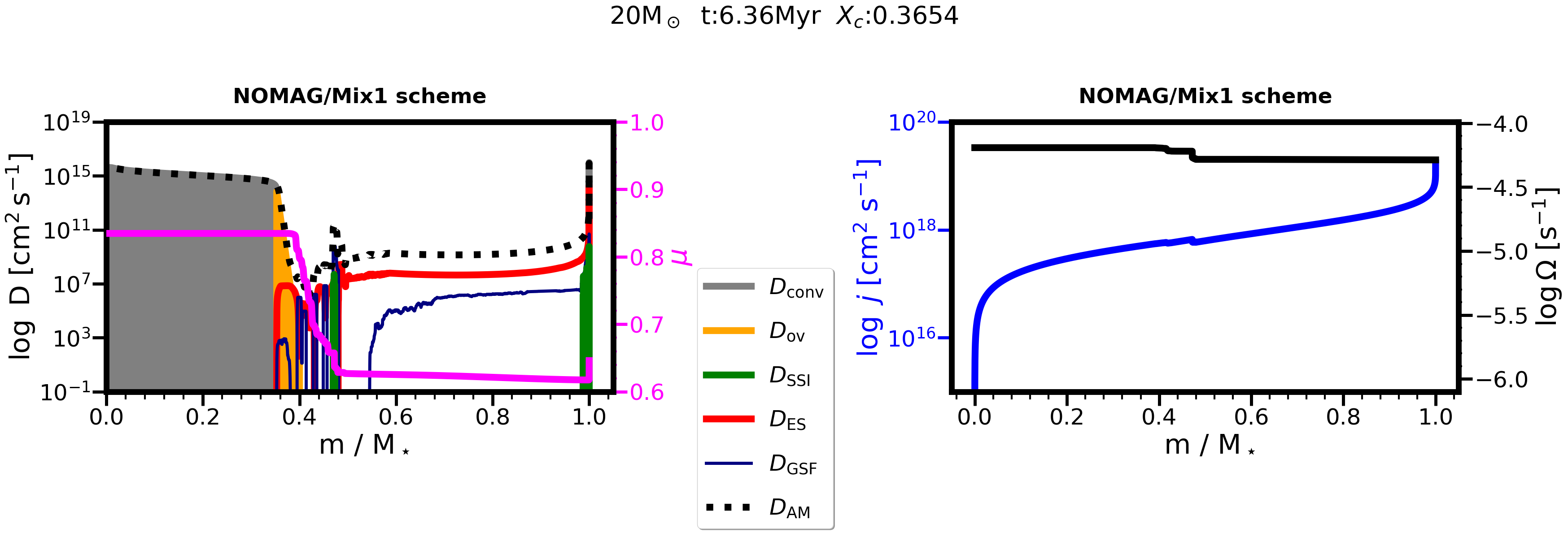
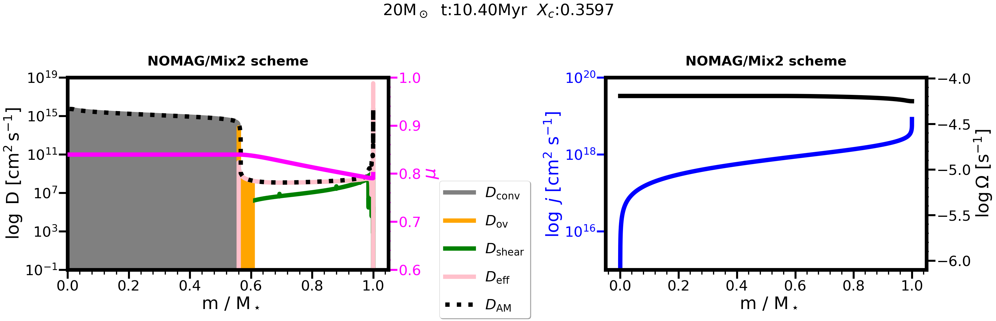
Figure 2: We show a non-magnetic model of $M_{\rm ini}$ = 20 M_⊙ (at $Z=0.014$) within the NOMAG/Mix1 scheme (top panel) and an initially identical model within the NOMAG/Mix2 scheme (lower panel) at half-way through its core hydrogen burning phase (with core hydrogen mass fraction of $X_{\rm c}/X_{\rm c,init}\approx 50\%$). Left: diffusion coefficients for chemical mixing (solid lines for rotational mixing and shaded grey and orange for convective core mixing and overshooting, respectively; all entering via $D_{\rm chem}$ in Equation 12) and diffusion coefficient for angular momentum transport (dotted line, entering Equation 11). The right ordinate and magenta line show the mean molecular weight. Due to the stochastic nature of mixing processes and, in some cases, numerical noise, here and hereafter we apply a moderate smoothing of some diffusion coefficients for visualisation purposes. Right: Specific angular momentum (left ordinate, blue line) and angular velocity (right ordinate, black line).

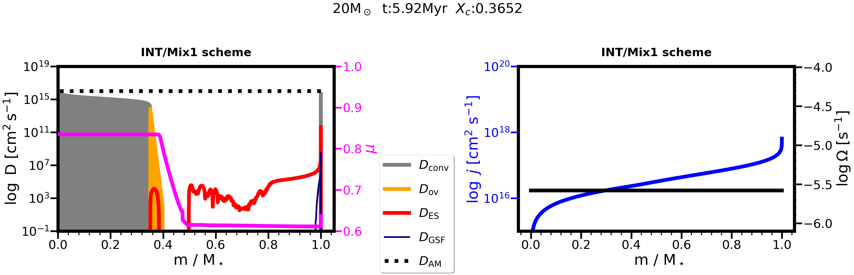
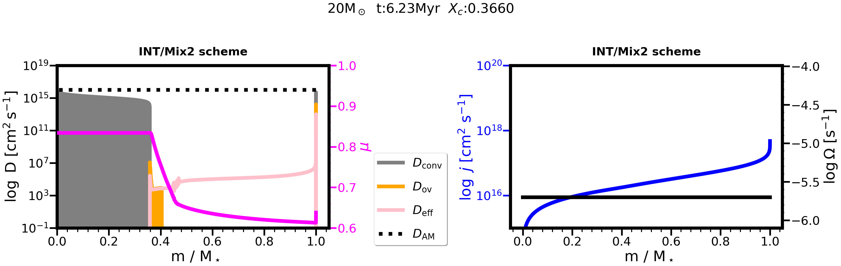
Figure 3: Same as Figure 2 but for magnetic models within the INT magnetic braking scheme.

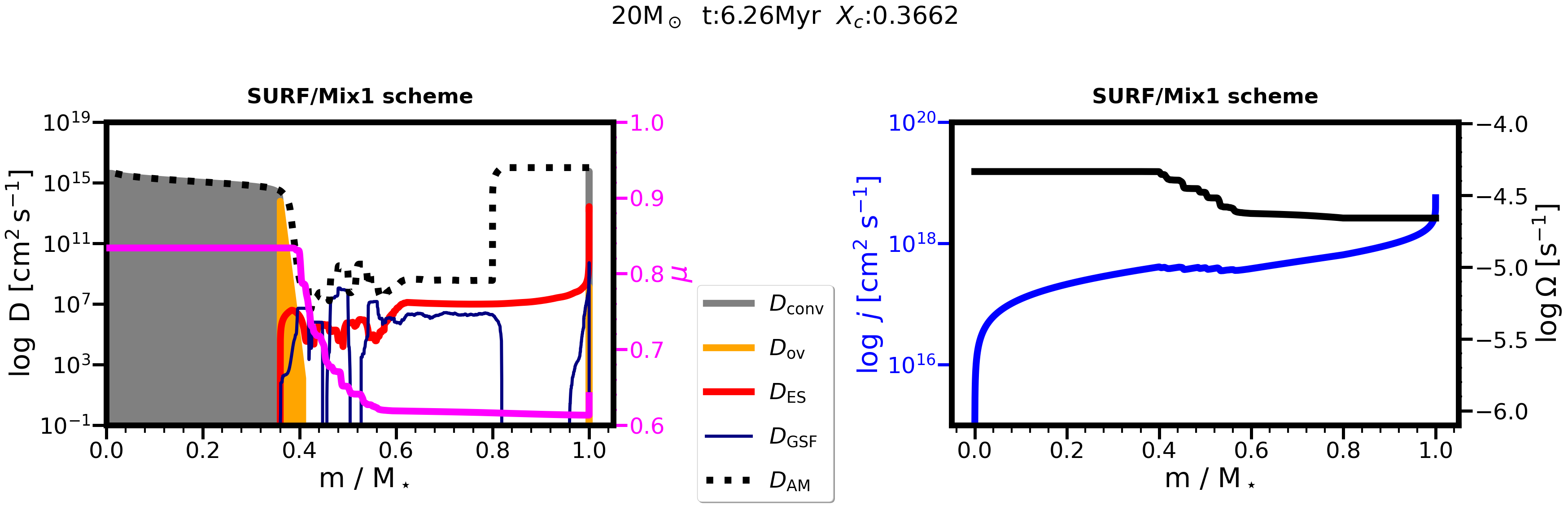
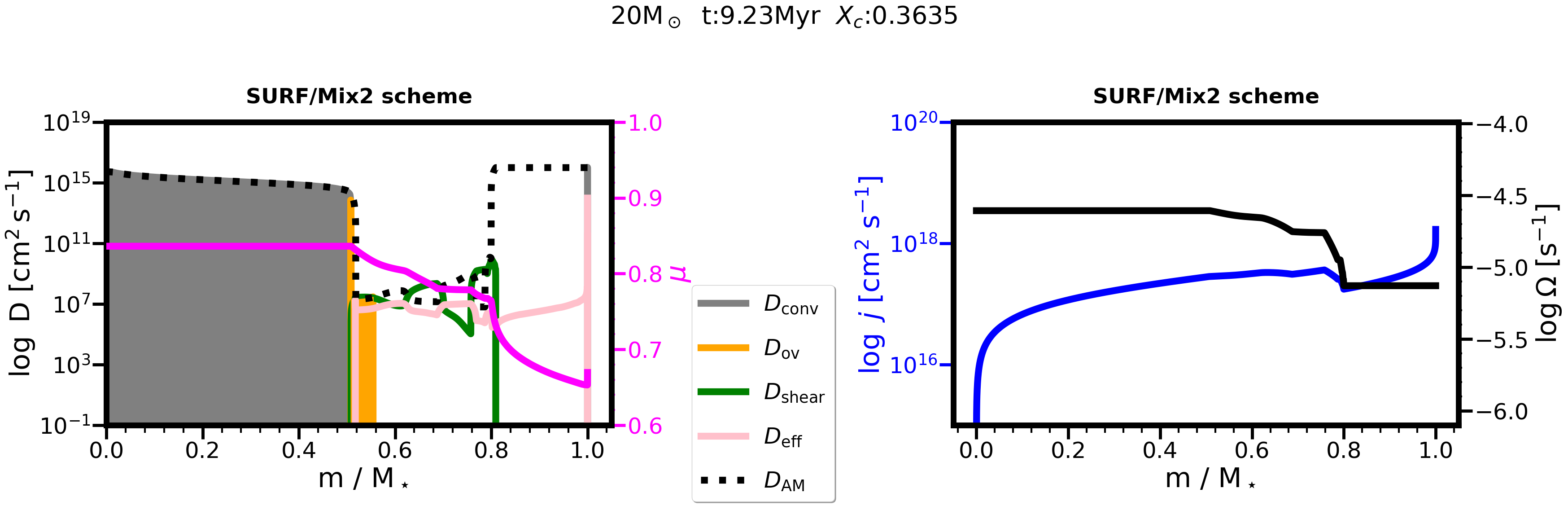
Figure 4: Same as Figure 2 but for magnetic models within the SURF magnetic braking scheme.

3.1 Stellar structure models

3.1.1 Chemical mixing and angular momentum transport

Figures 2, 3, and 4 show 20 M_⊙ models at solar metallicity. These structure models are at half-way through their core hydrogen burning phase (defined as $X_{\rm core}/X_{\rm core,init}=0.5$). In Figure 2, we show non-magnetic models in the Mix1 (top panel) and Mix2 (lower panel) chemical mixing schemes. (Since magnetic braking is not applied, there is no braking scheme in these cases, hence we refer to these models as "NOMAG".) In Figure 3, the fiducial model (INT/Mix1, top panel) as well as an otherwise initially identical model but within the INT/Mix2 scheme (lower panel) is shown. Models with the SURF/Mix1 and SURF/Mix2 schemes are shown in Figure 4. Note that the models with the adopted braking and mixing schemes correspond to different stellar ages when the core hydrogen is half-way depleted in each model (indicated in the title of the panels), given the different evolution resulting from the change in physical assumptions.

When fossil magnetic fields are not considered in the models (NOMAG case; $B_{\rm eq}=0$), the Mix1 and Mix2 chemical mixing schemes produce drastically different results. In the Mix1 scheme, the mean molecular weight (shown with magenta line and on the right ordinate) drops rapidly at the convective core boundary (the zones with convective overshooting are shown with orange in Figure 2). Near this region the GSF instability dominates (see, e.g., the recent studies of Caleo et al. 2016; Barker et al. 2019, 2020; Chang & Garaud 2021). Once the chemical composition is stabilised, meridional circulation drives chemical mixing (red line) and angular momentum transport (dotted line). Note that the assumption of $f_{\rm c}=0.033$ reduces the efficiency of all instabilities considered for chemical mixing compared to the efficiency of the same instabilities used for angular momentum transport. The angular velocity profile (right panel) remains completely flat in the stellar envelope, with a small break at the core boundary. Thus the model is very close to solid-body rotation. The NOMAG/Mix2 model reveals a very efficient mixing, with an almost flat mean molecular weight profile indicating close-to chemically homogeneous evolution. The dominant transport is via the effective diffusion coefficient (Equation 17). Importantly, the diffusion coefficients at the core-envelope boundary are smooth. This is a critical region that allows for mixing up material from the core to the surface. Note the much larger convective core (in grey) compared to the Mix1 model. The specific angular momentum (blue line, right panel) and angular velocity profiles are smooth throughout the star. $\Omega$ slightly decreases near the surface as a result of mass loss, however, this model is also very close to solid-body rotation.

In the INT braking scheme (Figure 3) the angular velocity profile is completely flat. The star is rigidly rotating due to the assumed high diffusivity for transporting angular momentum attributed to the magnetic field, albeit the angular rotation is much lower than in the NOMAG model due to magnetic braking (uniformly) lowering the specific angular momentum. The rigid rotation does not allow shears to develop and transport angular momentum or chemical elements. Therefore in these models the chemical enrichment is entirely driven by meridional currents. In the "standard" mesa description (Mix1 scheme) a gap in the transport develops above the overshooting region, corresponding to steep chemical gradients, as seen from the large drop of the mean molecular weight (magenta line, right ordinate) at the core boundary. Despite the mitigating effect of $f_{\mu}=0.1$ in these models, the inefficient mixing above the core boundary will prevent a very efficient surface enrichment and overall mixing inside the star. If the gap existed throughout the entire early evolution, it would completely inhibit surface enrichment. However, the gap is not present initially – see top panels of Figures 14 and 15 –, when the mixing and corresponding enrichment are prominent. With internal magnetic braking, all layers of the star lose angular momentum, therefore the shape of the specific angular momentum profile remains unchanged whereas its overall value decreases over time. In the Mix2 scheme, $D_{\rm eff}$ never becomes zero close to the convective core. This allows for a smoother composition gradient and more overall mixing, therefore differences in surface abundances are expected. On the other hand, the specific angular momenta are not so different between the Mix1 and Mix2 schemes in the INT models. $\Omega$ is smaller in the Mix2 model, but this quantity also depends on the radius of the star. Since the model in the INT/Mix2 scheme takes more time than the INT/Mix1 to deplete hydrogen in its core due to the more efficient chemical mixing, at half-way through its core burning stage it has a larger radius. We also note that the NOMAG/Mix2 model produces a more efficient mixing than the INT/Mix2 model. As a consequence, the INT/Mix2 model results in a smaller convective core than the non-magnetic case.

In the SURF braking scheme (Figure 4), one major difference is that there is no overall solid-body rotation. Let us recall that in the SURF models only the outer layers enclosing the top 20% of the total mass of the star are assumed to lose angular momentum (see Equation 10) and have an increased diffusivity for angular momentum transport (via Equation 11). In a 1D diffusive scheme, angular momentum flows from inner to outer layers. The angular velocity profile is flat in those layers where the diffusivity is increased. Depending on the mixing scheme, the composition and also the mixing processes are rather different. The magnitude and radial dependence of the diffusion coefficient for angular momentum transport also determines the angular velocity in the rest of the stellar envelope. We see that in the SURF/Mix1 model the angular velocity is also roughly constant between 0.6 and 0.8 $m/M_{\star}$, and it gradually changes closer to the boundary of the stellar core, as it is the case for $D_{\rm AM}$ (left panel, dotted line). In the SURF/Mix2 model, $D_{\rm AM}$ changes more abruptly at around 0.8 $m/M_{\star}$, whereas it is roughly constant again closer to the stellar core. Braking for a given magnetic field strength is less efficient in the SURF scheme than in the INT scheme since the Alfvén radius is smaller for a quadrupole field than for a dipole field as defined by Equations 3-5. Given the shape of the specific angular momentum profile (right panel, blue line), the SUFR/Mix1 model has a break closer to the stellar core, while the SURF/Mix2 model has a break closer to 0.8 $m/M_{\star}$. This means that the SURF/Mix2 model can more easily exhaust its surface reservoir of angular momentum.

Certainly, further research is required to investigate how angular momentum transport and magnetic braking work for more complex magnetic field configurations and how they could be implemented in 1D stellar evolution models. Overall, the results from the SURF approach may be considered similar to the works of Meynet et al. (2011) and Paper I, where magnetic braking was only applied to the uppermost stellar layer.

In the SURF/Mix1 scheme, the GSF instability can efficiently transport chemical elements near the core boundary. This instability acts on a dynamical timescale and therefore can vary from timestep to timestep. In the upper envelope meridional currents remain efficient. In the Mix2 scheme, the free parameters controlling mixing efficiency are not applied ($f_{\mu}=1$, $f_{\rm c}=1$), and the SURF/Mix2 scheme is thus the most efficient in chemical mixing. This is also evidenced by the larger convective core size compared to the three models in the other magnetic schemes. In fact, the convective core size of the SURF/Mix2 model is similar to that of the NOMAG/Mix2 model. Strong gradients of chemical elements do not develop near the core boundary. Shear mixing remains efficient in the entire envelope to transport chemical elements.

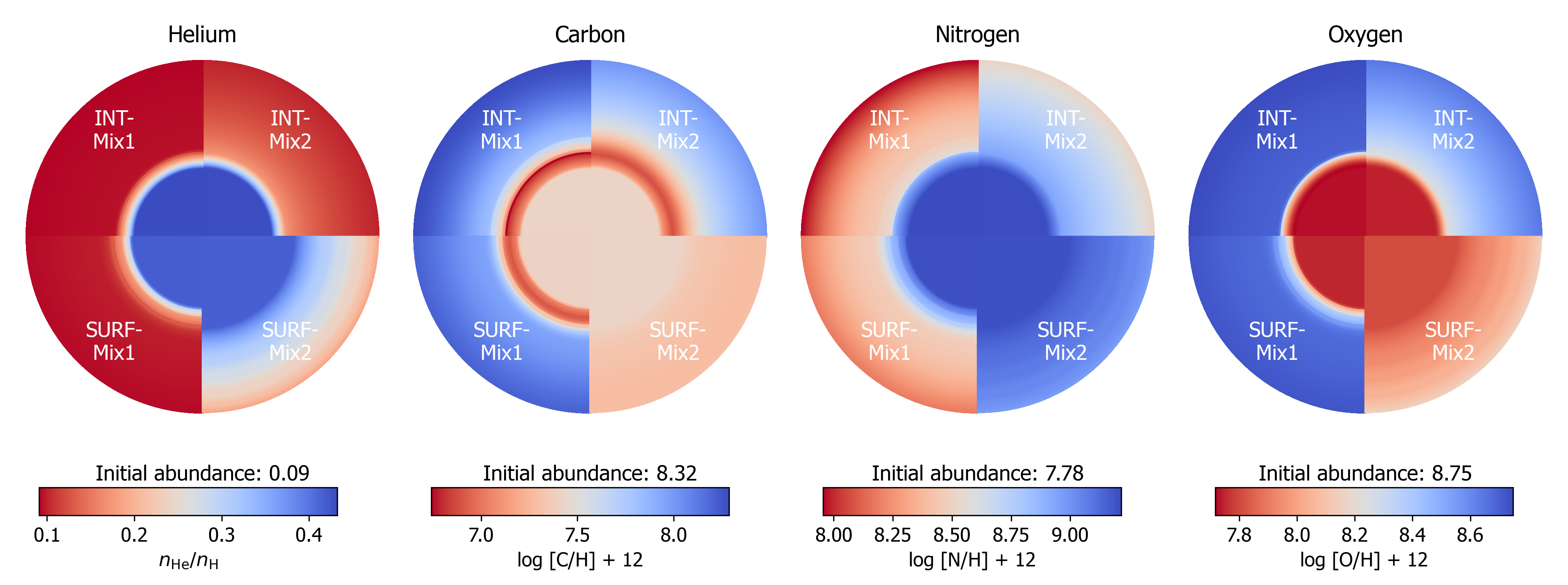
Figure 5: He, C, N and O abundances for the same models as in Figures 3 and 4 at $X_{\rm c}\approx 0.36$. In each circle, colour maps show the abundance of one element as a function of stellar mass coordinate, where the distance from the centre of the circle corresponds linearly to the mass enclosed within that radius. Each quarter circle contains the abundance profiles of one model. He abundance is in number fraction, the other elements in logarithmic number fractions. These profiles are prepared using tulips (Laplace, 2021).

3.1.2 Abundances of He, C, N, O

Figure 5 shows the abundances of helium, carbon, nitrogen, and oxygen. For three models (INT/Mix1, INT/Mix2, SURF/Mix1) the convective hydrogen core sizes are comparable. The SURF/Mix2 scheme, which is the most efficient in mixing, leads to a much larger core. In this model, the average helium content in the stellar envelope is much higher and the surface will also show this increased abundance already on the main sequence. Carbon is slightly depleted during the CNO-cycle (it becomes most depleted in a thin layer close to the core boundary), however the surface carbon abundance is minimally changed in the first three models. In contrast, the SURF/Mix2 model produces an almost uniform distribution of carbon inside the star, it is completely mixed in the envelope without any gradients. Nitrogen excess is produced during the CNO-cycle, and therefore, its surface abundance is a crucial measurement to infer the efficiency of internal mixing. All models produce a surface nitrogen enrichment, except the INT/Mix1 scheme. Here a strong gradient develops between the core and the surface. While a core-surface gradient is also present in the INT/Mix2 and SURF/Mix1 models, their envelopes have a somewhat higher mean nitrogen abundance and their surfaces are slightly enriched in nitrogen. The SURF/Mix2 model has an almost homogeneous nitrogen distribution in its envelope. Oxygen is depleted during the CNO-cylce. Similar to carbon, oxygen can still remain abundant in the envelope in the first three models. The SURF/Mix2 model yields a close-to-homogeneous oxygen distribution throughout the star. In contrast to carbon, in all four models oxygen is depleted in the entire stellar core. For example, the core to surface oxygen abundance can differ by an order of magnitude in the INT/Mix1 model.

The reason why strong gradients can develop (and remain in most models) near the core boundary is related to the drop in chemical mixing, identifiable by drops and gaps in the diffusion coefficients (c.f. Figures 3-4), which in turn depend on the composition gradients. The velocity of the diffusion is zero when there is no composition gradient and it increases when the gradient increases. This is another effect that leads to reducing the diffusion coefficient. For helium, the difference between the core and the envelope grows gently, while for nitrogen it grows faster because nitrogen is enhanced very rapidly in the core. Thus for a given diffusion coefficient, nitrogen will diffuse more rapidly than helium. In the Mix2 scheme, the key differences between the INT and SURF models result from their different angular velocity profiles. The INT models lose angular momentum in all layers and thus mixing becomes less efficient overall. The SURF/Mix2 model has a more massive convective core at the same evolutionary stage (c.f. Figure 4), and the envelope closely reflects on the core composition as this model has an almost homogeneous distribution of chemical elements. In both INT/Mix1 and INT/Mix2 schemes, envelope mixing has a similar overall efficiency. However, in the INT/Mix2 scheme, the near core mixing is more efficient (see above), greatly impacting the measurable surface abundances of carbon, nitrogen and oxygen. The surface abundances, especially of nitrogen, are sensitive to the chosen braking and mixing schemes, especially with the Mix2 scheme reflecting more closely the core composition than the Mix1 scheme.

3.2 Evolutionary tracks

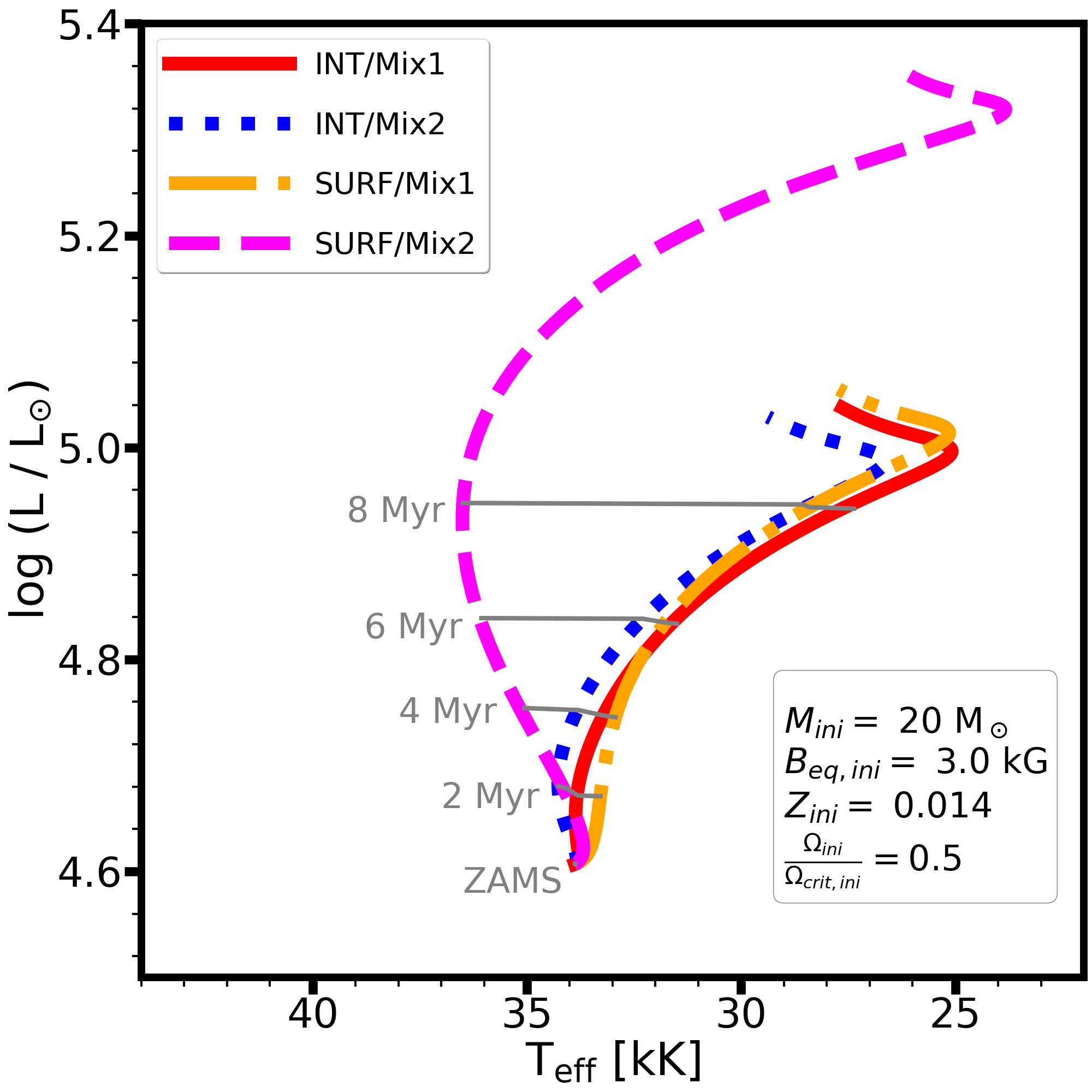
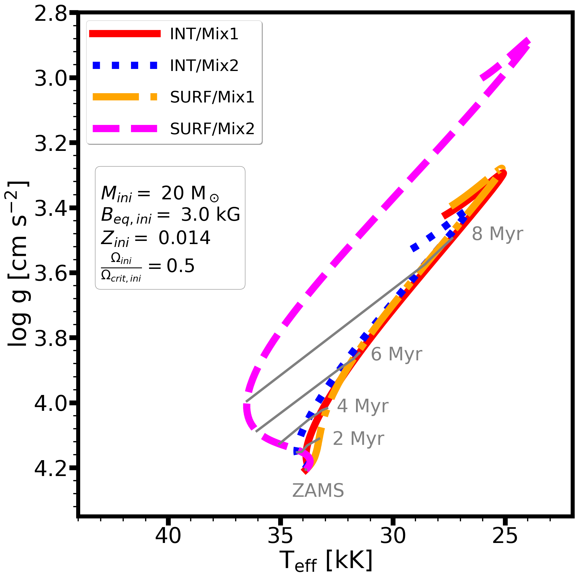
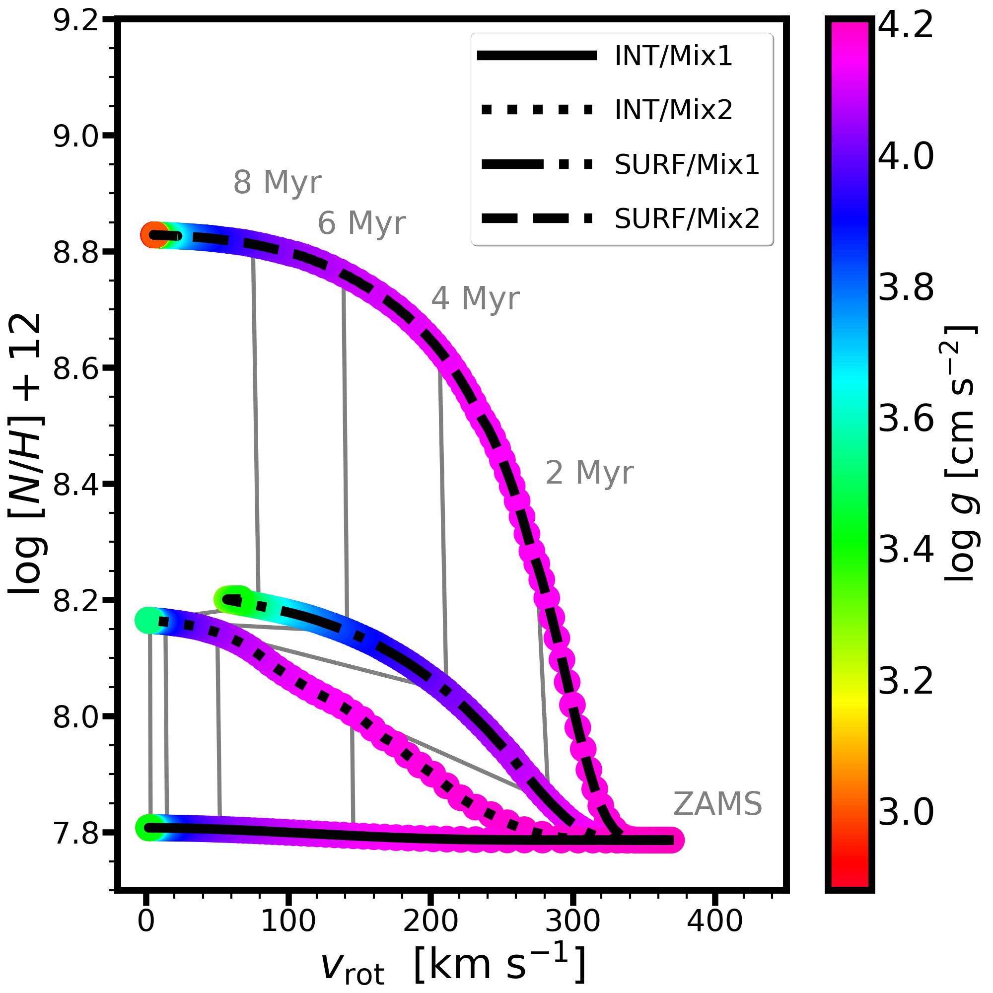
Figure 6: Fiducial evolutionary model with $M_{\rm ini}=$  20 M_⊙ at $Z=0.014$ with $B_{\rm eq,ini=}$ 3 kG within the INT/Mix1 scheme and the 3 other schemes, indicated with different colours and line-style. Grey lines connect equal ages. Panels from left to right show the HR, Kiel, and Hunter diagrams, respectively. The colour-coding shows the logarithmic surface gravity on the Hunter diagram.

3.2.1 Impact of magnetic braking and chemical mixing schemes for 20 M_⊙ models

Figure 6 shows the fiducial 20 M_⊙ model (INT/Mix1) as well as initially identical models but in the other 3 schemes in the HRD, Kiel diagram, and Hunter diagram (Hunter et al., 2008, 2009). Here we address the impact of using the different braking and mixing schemes for otherwise identical models with the same initial mass and initial magnetic field strength.

The models within the Mix1 chemical mixing scheme result in closely overlapping tracks on the HRD and Kiel diagrams. However, as evidenced from the Hunter diagram (right panel of Figure 6), the spin-down and chemical enrichment are different when considering the different magnetic braking schemes. The 20 M_⊙ INT/Mix1 model (solid line) produces essentially no observable surface nitrogen enrichment in this configuration. The SURF/Mix1 model (dashed-dotted line), on the other hand, maintains a higher angular velocity in the inner regions of the star by braking only the upper layers (see Section 3.1). This is why mixing remains more efficient and a larger amount of nitrogen is mixed to the stellar surface (0.45 dex). Model predictions within the Mix2 chemical mixing scheme produce a much more efficient chemical mixing than the Mix1 scheme. However, the differences between the INT/Mix2 and INT/Mix1 schemes are relatively modest on the HRD and Kiel diagrams, while the Hunter diagram shows large deviations. The INT/Mix2 model reaches a surface nitrogen abundance that is about 0.4 dex higher than the baseline value.

Contrary to the first three cases, the SURF/Mix2 model has an extended blueward evolution, shown on the HRD and Kiel diagrams. Such a feature is commonly associated with blue stragglers, merger products, and quasi-chemically homogeneous evolution (e.g., Maeder, 1987; Yoon et al., 2006; Knigge et al., 2009). Given the very efficient mixing in this model, it is nearly chemically homogeneous (c.f. Figure 5). Indeed, the SURF/Mix2 model produces the highest nitrogen enrichment, more than 1 dex compared to the baseline in this configuration.

Even without considering magnetic braking, the two mixing schemes are considerably different, which leads to different evolutionary tracks. The assumptions regarding the mutual effect of the magnetic field and chemical mixing allow for a range of behaviours (see also Paper III). Models within the Mix1 scheme have modest differences as a result of using the different braking schemes (INT/SURF). Models within the Mix2 scheme produce very efficient mixing, which is more easily quenched in the INT models than in the SURF models. The INT braking scheme, in contrast to the SURF, decreases the overall rotation rate, and the INT/Mix2 models do not evolve significantly blueward on the HRD. However, quasi-chemically homogeneous evolution is achieved in the case of non-magnetic Mix2 models, as well as in some magnetic SURF/Mix2 models depending on the initial field strength and stellar mass (see Figs. 20 and 21, in the Appendix). For example, the magnetic model in the SURF/Mix2 scheme leads to quasi-chemically homogeneous evolution for most of the main sequence ($\approx 9$ Myr out of 12 Myr) of a 20 M_⊙ model at solar metallicity with a 3 kG magnetic field. However, for the same initial field strength, the initially 60 M_⊙ model only experiences a brief phase of quasi-chemically homogeneous evolution and then evolves redwards (Figure 21).

In summary, the braking and mixing schemes can drastically change the main observable characteristics. For example, the 8 Myr isochrone spans over a 10 kK effective temperature range (left panel of Figure 6) despite the models being initially completely identical. (When the "extreme" case of SURF/Mix2, which is assumed to represent stars with complex magnetic fields and very efficient mixing, is not considered the difference is less, around 2 kK.) Thus the uncertainties associated with braking and mixing schemes in evolutionary model predictions are significant. From the Hunter diagram we can conclude that various braking and mixing schemes can cover a wide range of rotation rates and surface nitrogen abundances. Three models already reach slow rotation ($<50$ km s^-1) with high surface gravities. Both INT models take less than 6 Myr to achieve this, while it is slightly over 8 Myr for the SURF/Mix2 model. The SURF/Mix1 model reaches the TAMS with a somewhat higher rotation rate than the other models.

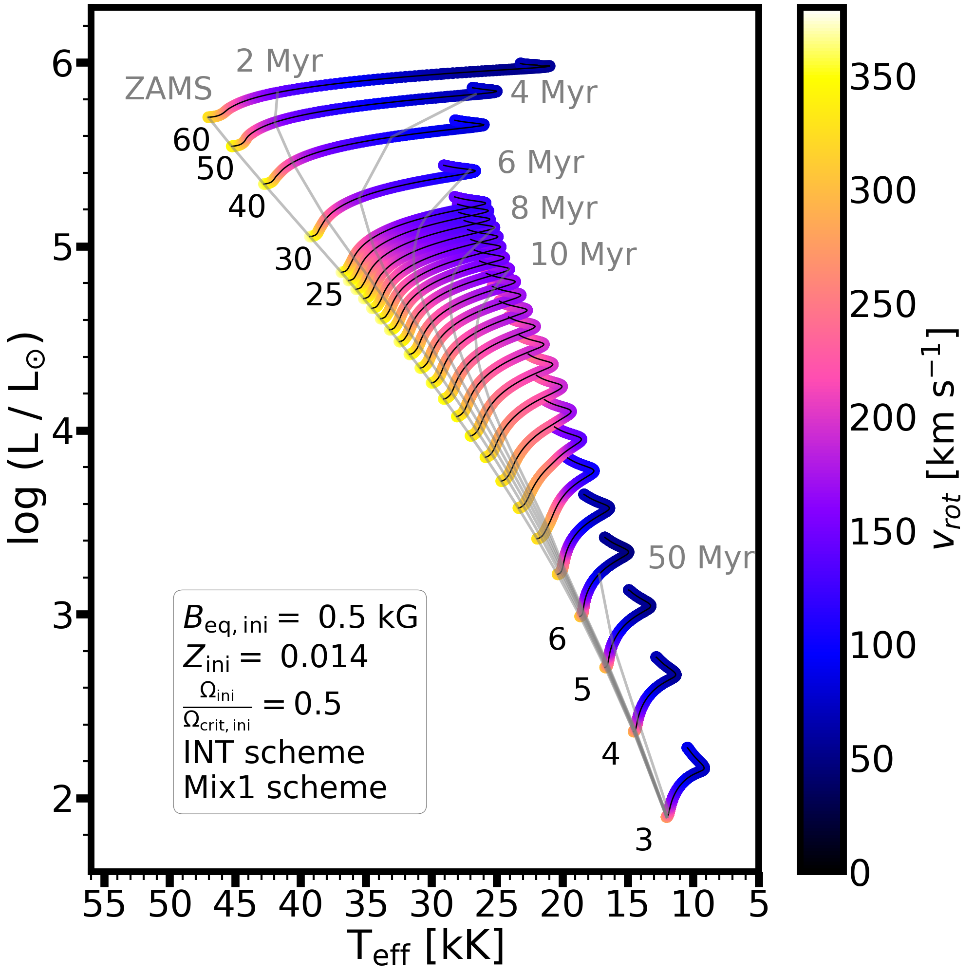
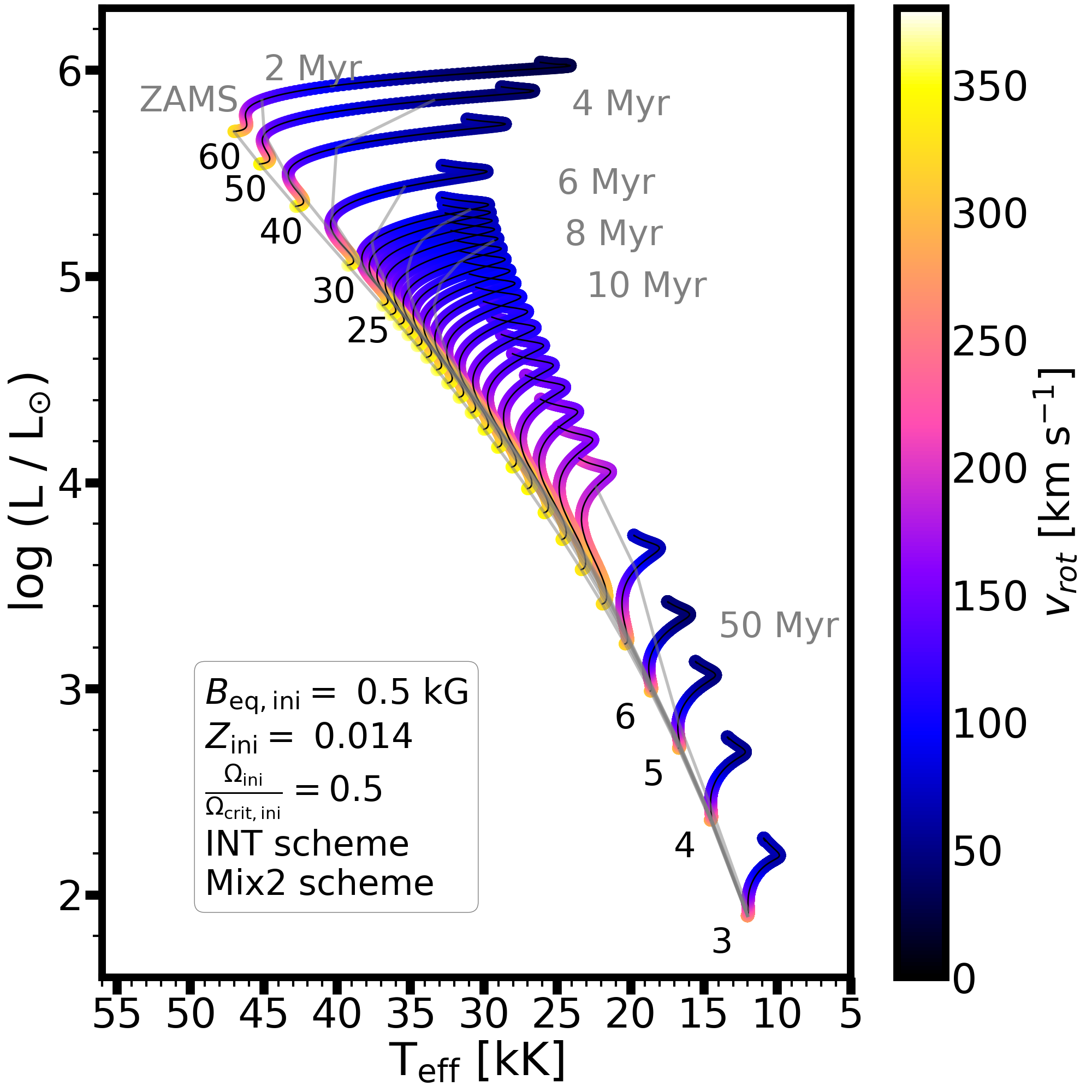
Figure 7: Hertzsprung-Russell diagram of magnetic single-star evolutionary models with initial magnetic field strength $B_{\rm eq,ini}=0.5$ kG, initial rotation rates of $\Omega_{\rm ini}/\Omega_{\rm ini,crit}=0.5$ at solar $Z_{\rm ini}=0.014$ metallicity within the INT/Mix1 scheme (left) and INT/Mix2 scheme (right). The SURF schemes are shown in Figs. 19 and 21 in the Appendix. Isochrones with grey lines indicate the time evolution from ZAMS to 50 Myr. The initial masses in solar units are given next to the ZAMS of the models (between 6 and 25M_⊙, the increment is 1 M_⊙). The colour-bar shows how the equatorial rotational velocity evolves.

3.2.2 HRD evolution of a grid of magnetic models

Figure 7 shows the model predictions on the HRD colour-coded by the surface equatorial rotational velocity. Here the INT/Mix1 and INT/Mix2 schemes are displayed (see Figs. 19 and 21 in the Appendix for the SURF schemes) and we demonstrate the impact of a magnetic field with an initial equatorial field strength of 500 G.

In the INT models, strong magnetic braking leads to a rapid decrease of surface rotational velocity in the entire mass range from 3 to 60 M_⊙. This implies that rapidly-rotating (single) magnetic massive stars are expected to be young and close to the ZAMS on the HRD. Some quantitative differences arise from the assumptions of the chemical mixing schemes. Nonetheless, within the INT magnetic braking scheme these differences are small on the HRD, albeit it could affect the parameter determination (current age and mass) of known magnetic stars.

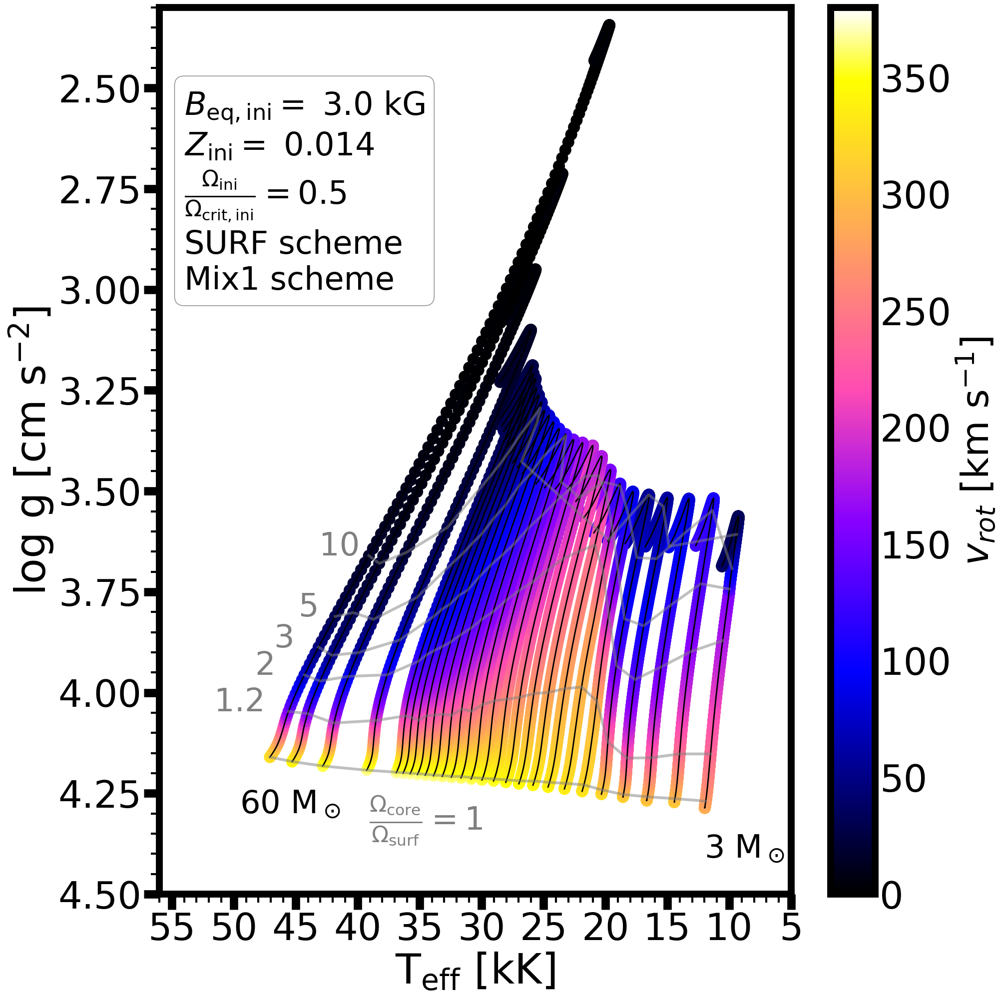
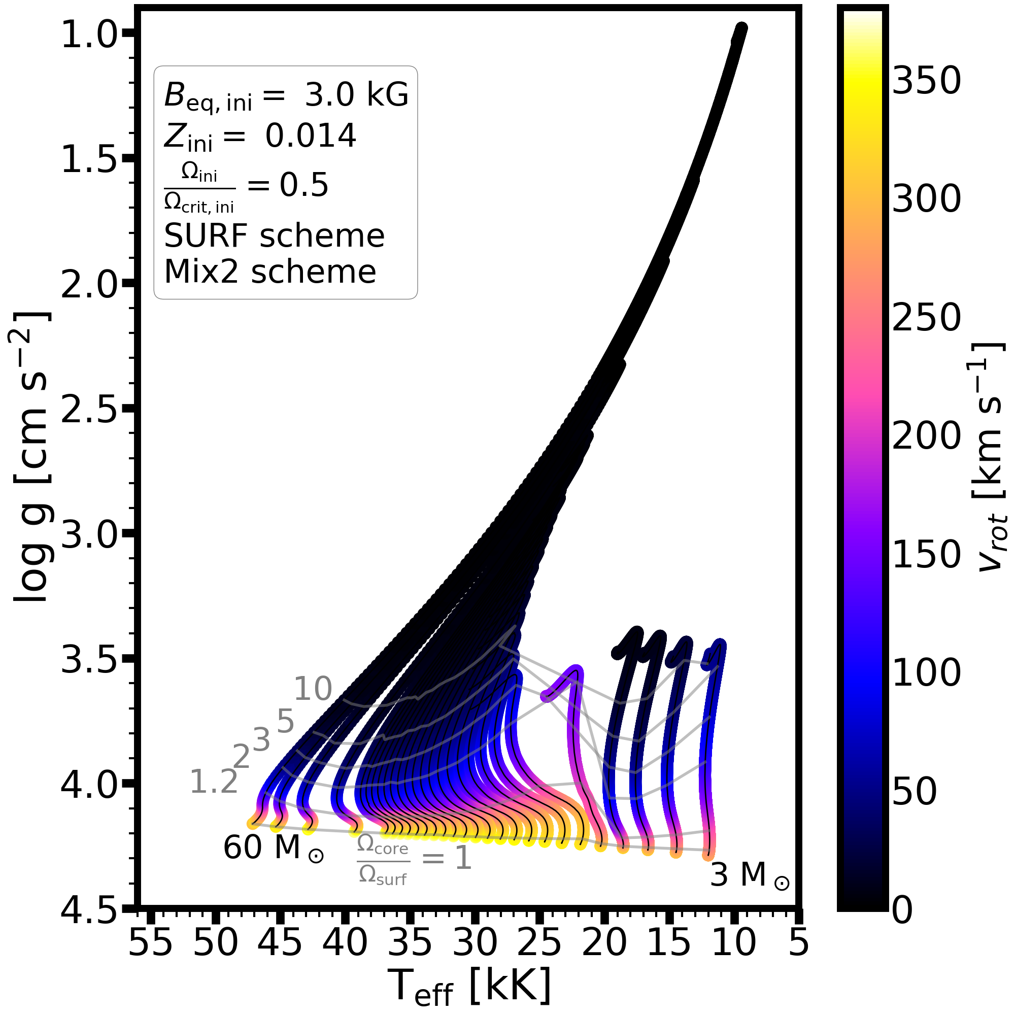
Figure 8: Kiel diagram of magnetic evolutionary models with $B_{\rm eq,ini}=3$ kG, $\Omega_{\rm ini}/\Omega_{\rm ini,crit}=0.5$ at solar metallicity $Z_{\rm ini}=0.014$. within the SURF/Mix1 (left) and SURF/Mix2 (right) schemes. Grey contour lines indicate the unitless degree of differential rotation, quantified as the ratio of core to surface angular velocity. Note that Figure 7 shows INT models where solid-body rotation ($\Omega_{\rm core}/\Omega_{\rm surf}=1$) is achieved throughout the main sequence (see also Figure 14). The initial masses of the models decrease from left to right. The colour-coding shows the surface equatorial rotational velocity.

3.2.3 Differential rotation on the Kiel diagram

Figure 8 shows the Kiel diagram. In the SURF models, radial differential rotation develops between the stellar core and surface, as indicated with the grey contour lines. This is because we assume that a magnetic field with a complex geometry would only exert a strong torque on the near-surface layers by considering that organised, strong magnetic flux is not present in deeper stellar layers (see also Braithwaite & Nordlund 2006; Braithwaite 2008). Thus angular momentum transport in the deepest layers of the stellar envelope is dominated by – less efficient – hydrodynamical instabilities. On the other hand, in the INT models complete solid-body rotation is maintained throughout the main sequence. Similar to Figure 6, where the 20 M_⊙ models are discussed, we see that the Mix1 and Mix2 chemical mixing schemes (within the SURF braking scheme here) result in notable differences in observable stellar parameters, which are the most prominent in the 5-10 M_⊙ range.

If the assumed magnetic field geometry remained unchanged throughout the main-sequence evolution, the prediction for magnetic massive stars is that differential rotation could be best identified in hotter, more massive, and more evolved (lower $\log g$) stars. An important caveat nevertheless is the time evolution of complex magnetic fields. According to Braithwaite (2008), complex fields may simplify to a dipolar form since higher-order harmonics diffuse more rapidly. Indeed, Shultz et al. (2019b) finds that evolved magnetic stars tend to have simpler geometries (however, see also Kochukhov et al. 2019). Insofar it remains unclear what the exact diffusion time of complex magnetic flux tubes would be (perhaps still longer than the main-sequence lifetime) and whether the corresponding effects which are modelled in evolutionary codes (angular momentum transport, magnetic braking, mass-loss quenching) would change significantly. We evaluated the models with different initial field strengths and found that a stronger magnetic field is able to achieve a higher degree of differential rotation in comparison to models with lower field strengths. It would therefore be of great importance to obtain seismic data of a sample of magnetic massive stars.

3.2.4 Mass-dependent rotational evolution

Both the HRD and Kiel diagrams presented above show the same distinctive feature. Namely, irrespective of how fast the spin-down per given scheme is, the mid-mass range models ($\approx$ 5-10 M_⊙, the transition typically taking place at around 5-7 M_⊙ depending on model assumptions) always maintain a higher rotational velocity than models with other masses. This is the most striking on the left panel of Figure 8 for the SURF/Mix1 scheme. (The exact model behaviour was also recognised for a 5 and 10 M_⊙ model in Paper II.) The distinctive feature is a consequence of the spin-down of the models, which does not scale linearly with mass. For higher-mass models, wind mass loss contributes to the spin-down. The spin-down time to reach a given surface rotation takes a lower fractional age when the mass increases for initial masses higher than 10 M_⊙. Since stars below about 5 M_⊙ have much longer nuclear timescales than higher-mass stars, even if magnetic braking is less efficient due to weaker winds, the available timescale allows for braking the rotation at a lower fractional main-sequence age. This results in stars below 5 M_⊙ rotating more slowly at the TAMS than in the 5-10 M_⊙ range. We emphasise that the extent of the tracks on the HRD is not linear with stellar age: a significant time evolution can take place in a narrow location on the HRD close to the ZAMS as demonstrated by the isochrones. For example, the 50 M_⊙ model spends the first 2 Myr of its evolution while decreasing its $T_{\rm eff}$ by only about 5 kK, whereas in the second 2 Myr of its evolution, its $T_{\rm eff}$ decreases by about 15 kK (Figure 7). Moreover, from 0 to 4 Myr, the 25 M_⊙ track evolves roughly 0.2 dex in luminosity and a few kK in $T_{\rm eff}$, which is a typical range of observational uncertainties depending on data quality and knowledge of distance and extinction. The precise age determination of young stars especially at initial masses below 25 M_⊙ becomes rather challenging with uncertainties well exceeding 1 Myr.

In summary, stars evolve slowly in the HRD at the beginning of the main sequence phase, and thus suffer strong magnetic braking while not evolving away from the ZAMS (in effective temperature and luminosity). However the interplay between the dependence on the initial mass of the meridional current velocity, the evolutionary timescale near the ZAMS and the evolution of the radius produces a small bump of the surface rotational velocity in the initial mass range of 5-10 M_⊙ (see also Paper II). At the TAMS, this gives rise to a slower rotational velocity in models below 5 M_⊙ than models in the mid-mass range.

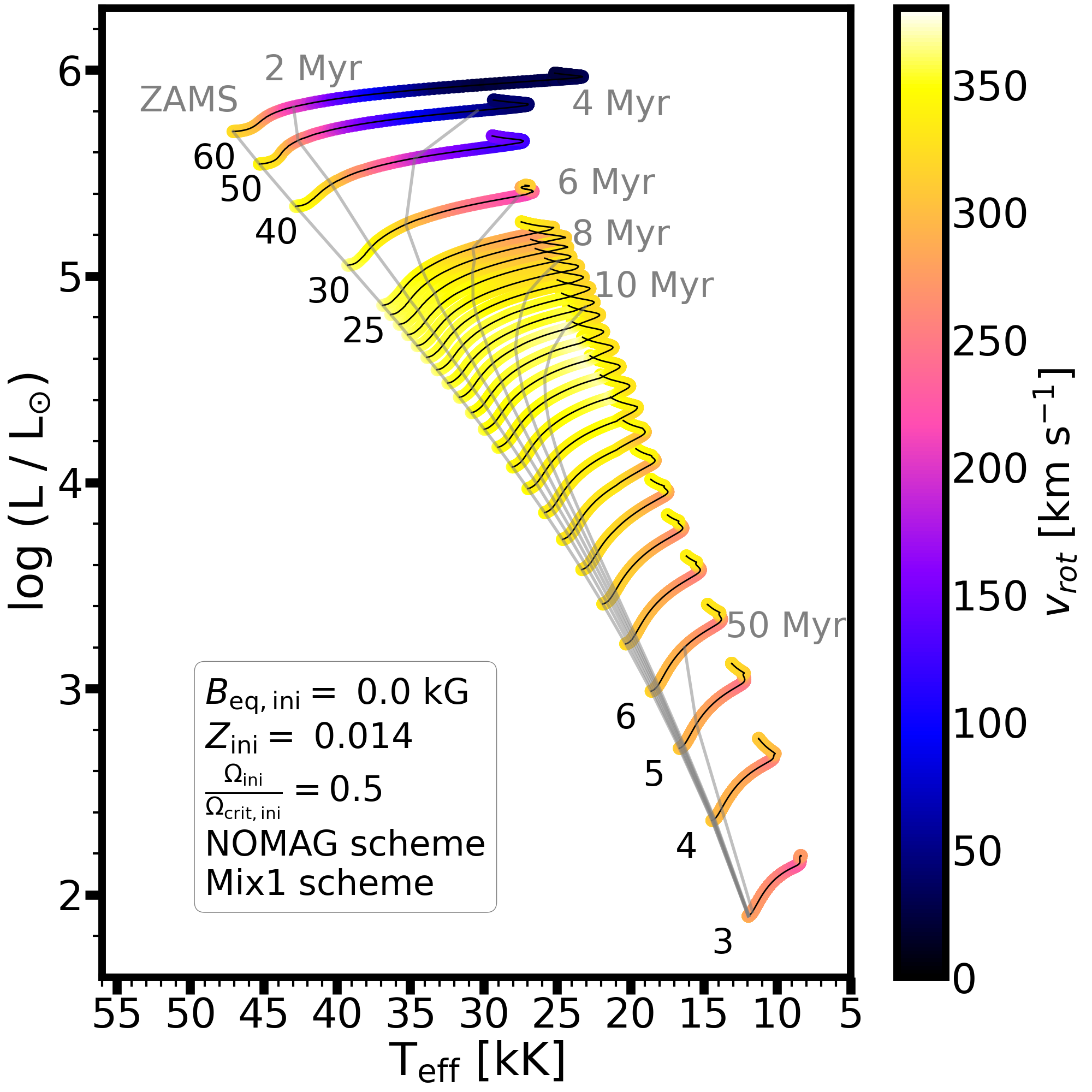
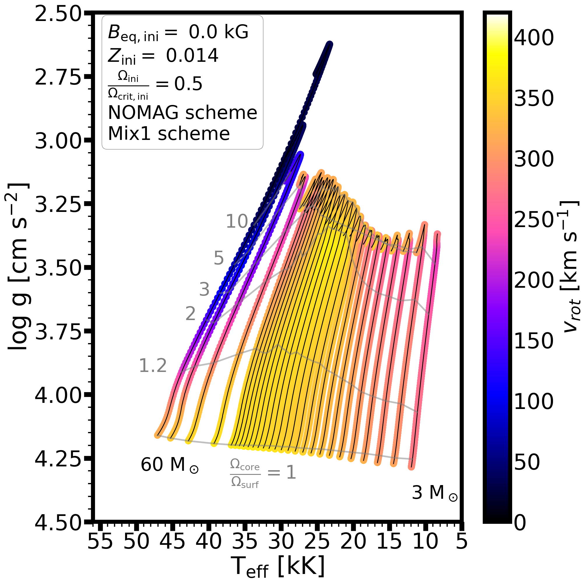
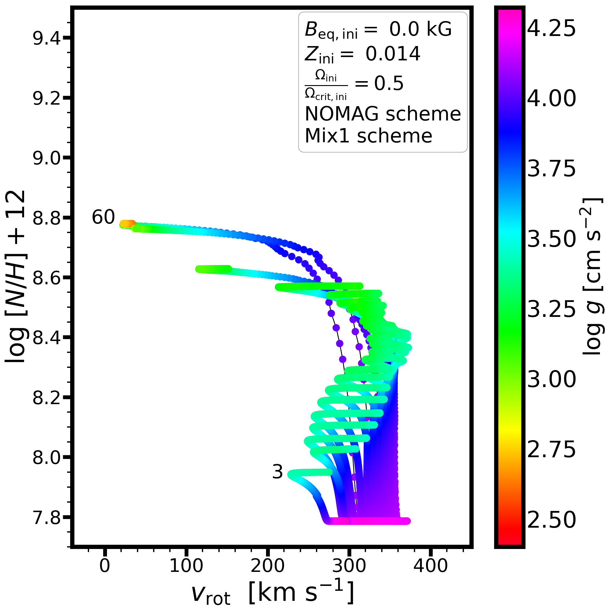
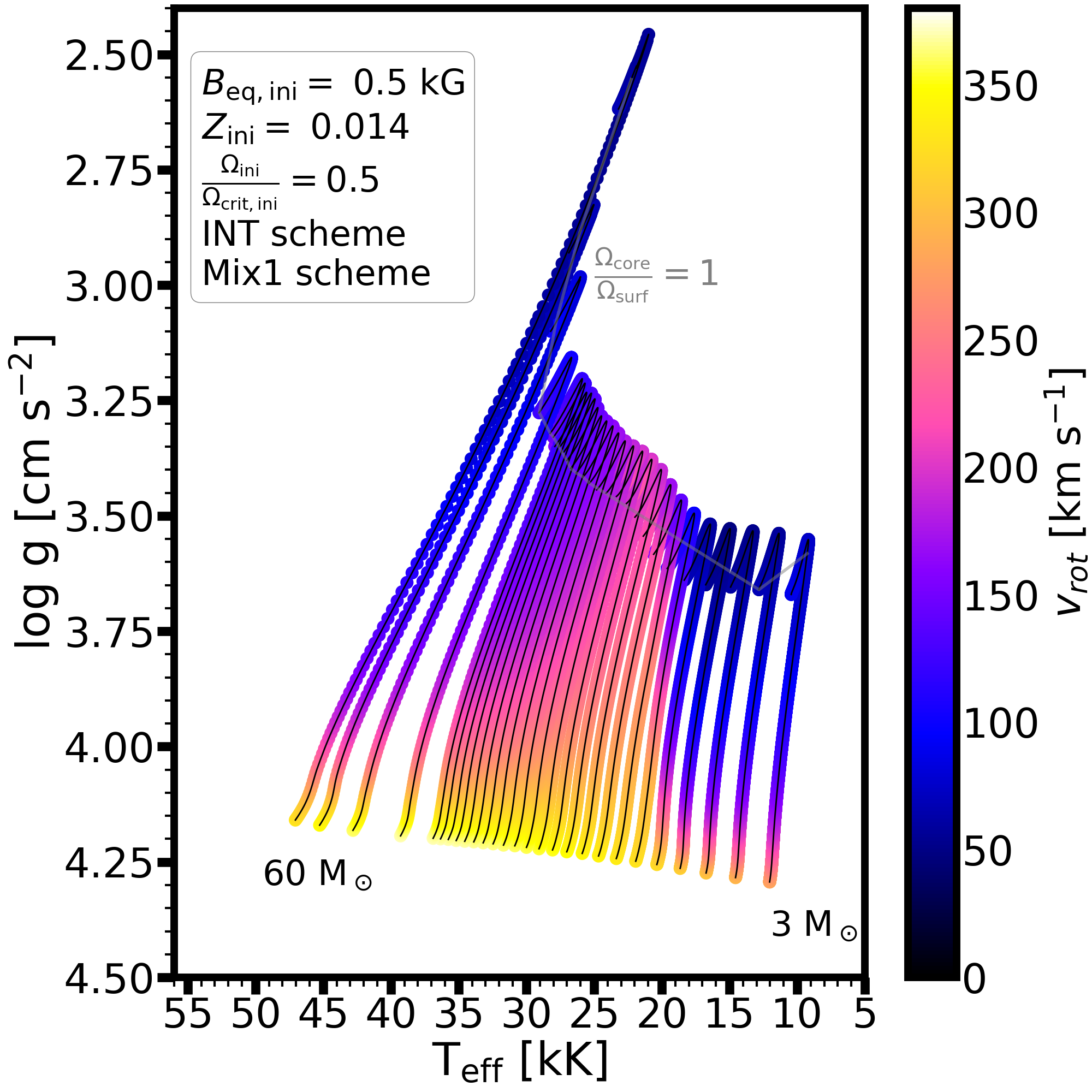
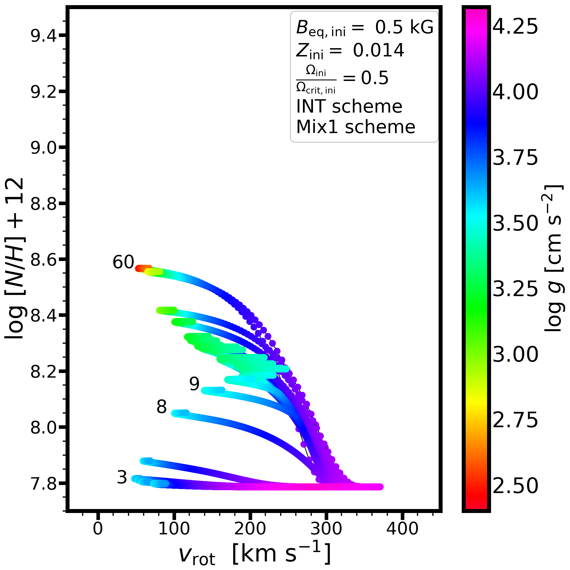
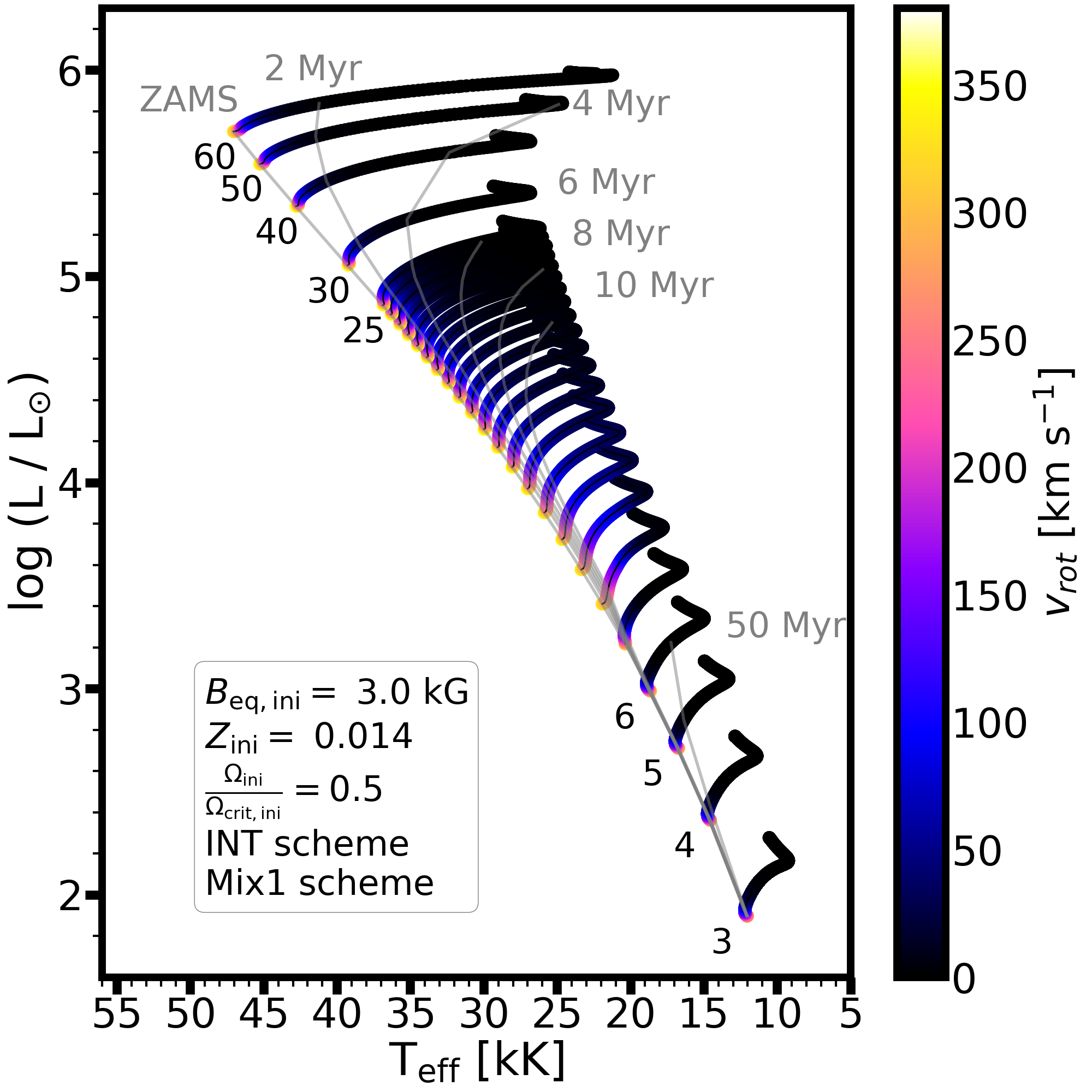
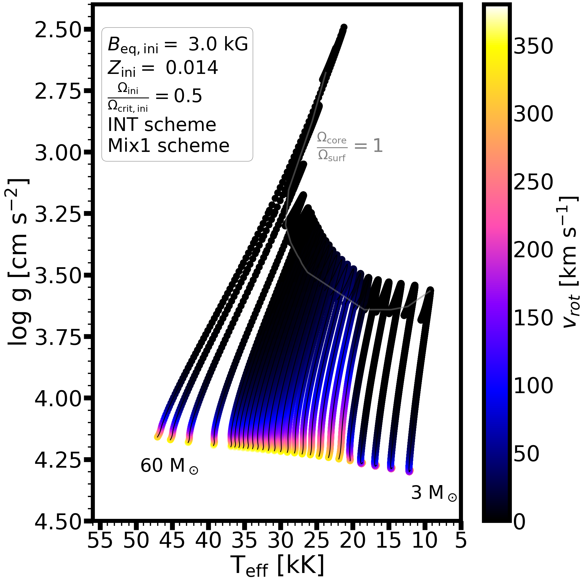
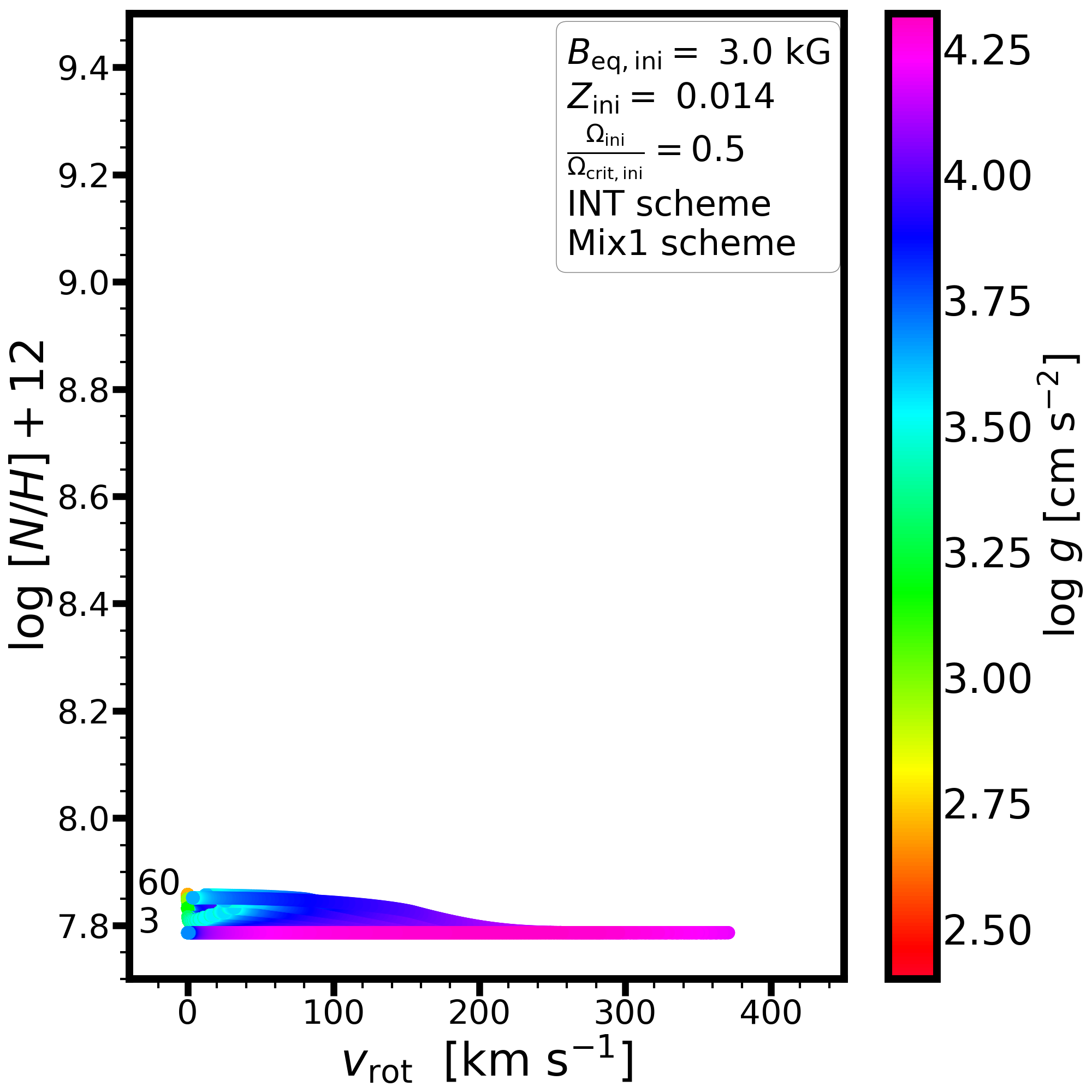
Figure 9: Evolutionary models from 3 to 60 M_⊙ at $Z=0.014$ with varying the initial equatorial magnetic field strength (0, 0.5, 3 kG from top to bottom), within the INT/Mix1 magnetic braking and chemical mixing schemes. Panels from left to right show the HRD, Kiel, and Hunter diagrams. The colour-coding denotes surface rotational velocity on the first two panels, while it denotes the logarithmic surface gravity on the right panel.

3.2.5 Impact of varying the initial equatorial magnetic field strength

Figure 9 shows the impact of the initial equatorial magnetic field strength within the INT/Mix1 scheme on the HRD, Kiel, and Hunter diagrams for models from 3 to 60 M_⊙. The colour-coding of the surface rotational velocity on the HRD and Kiel diagrams show that for initial masses above 30 M_⊙, stellar winds play a significant role in depleting the angular momentum reservoir, and thus even without magnetic fields those stars can significantly spin down on the main sequence. However, in the mass range from 3 to 30 M_⊙ single-star models would not undergo a dramatic angular momentum loss unless they were strongly magnetised. As demonstrated in the figure, the stronger the magnetic field, the more rapidly the surface rotation brakes. In particular, already a 3 kG equatorial field would produce a (sub)population of stars whose surface rotation is less than 50 km s^-1 throughout essentially the entire main sequence.

The Kiel diagram shows yet another consequence of magnetic fields. Apart from the highest-mass models ($>$ 30M_⊙), the models with stronger magnetic fields tend to reach the end of the main sequence with higher surface gravities. For example, for a 10 M_⊙ model, the TAMS value of $\log g$ increases from 3.3 to 3.4 and to 3.5 from the 0 kG to the 0.5 kG and to the 3 kG models, respectively. Non-magnetic models maintain a higher rotation and thus the mixing remains more efficient. This mixing (if not too strong to keep the star in a bluer position in the HRD) tends to enlarge the convective core and consequently, extend the width of the main sequence towards lower effective temperatures and higher surface gravities.

The Hunter diagram reveals that the magnetic models may strongly deviate from non-magnetic model predictions. The stronger the magnetic field, the more rapidly rotation brakes, and the less nitrogen can be mixed to the stellar surface. We identify and demonstrate that there exists a cutoff magnetic field strength, above which no surface enrichment is expected given that it leads to a shorter magnetic braking timescale compared to the rotational mixing timescale. However, this cutoff field strength is strongly model and parameter dependent, and thus the exact value varies for given stellar mass, initial rotation, metallicity, and mixing scheme, amongst others. We evaluate this in Section 4.2.

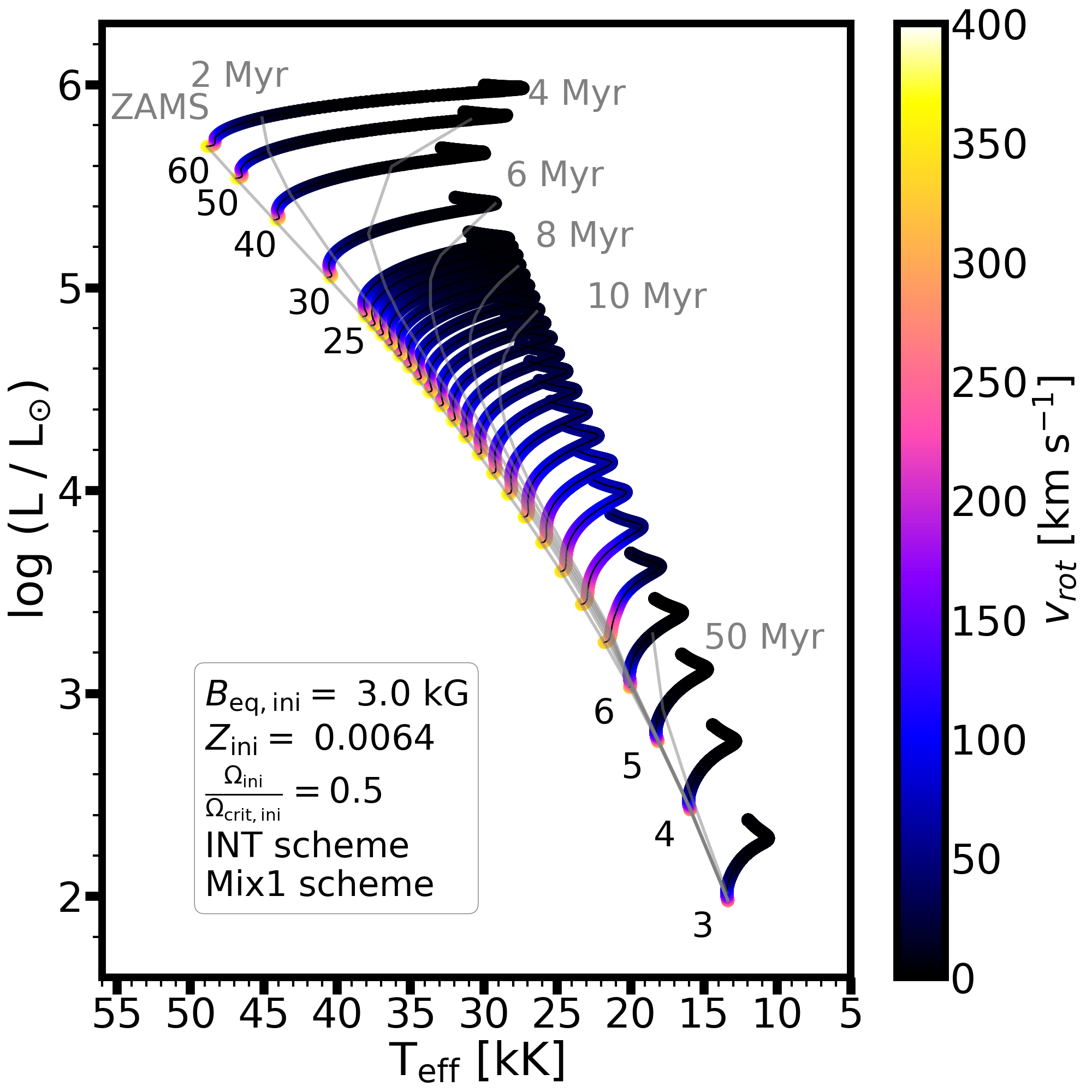
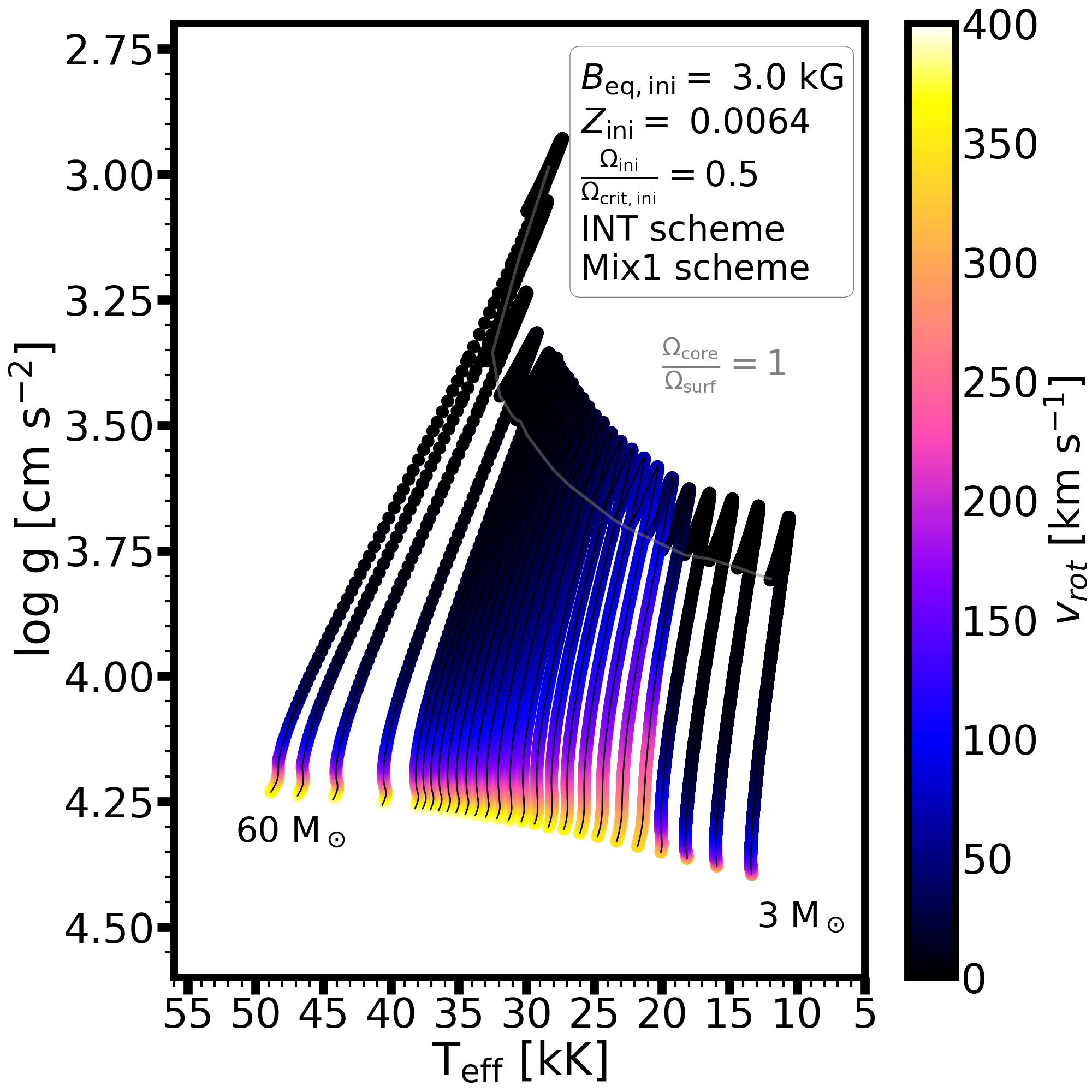
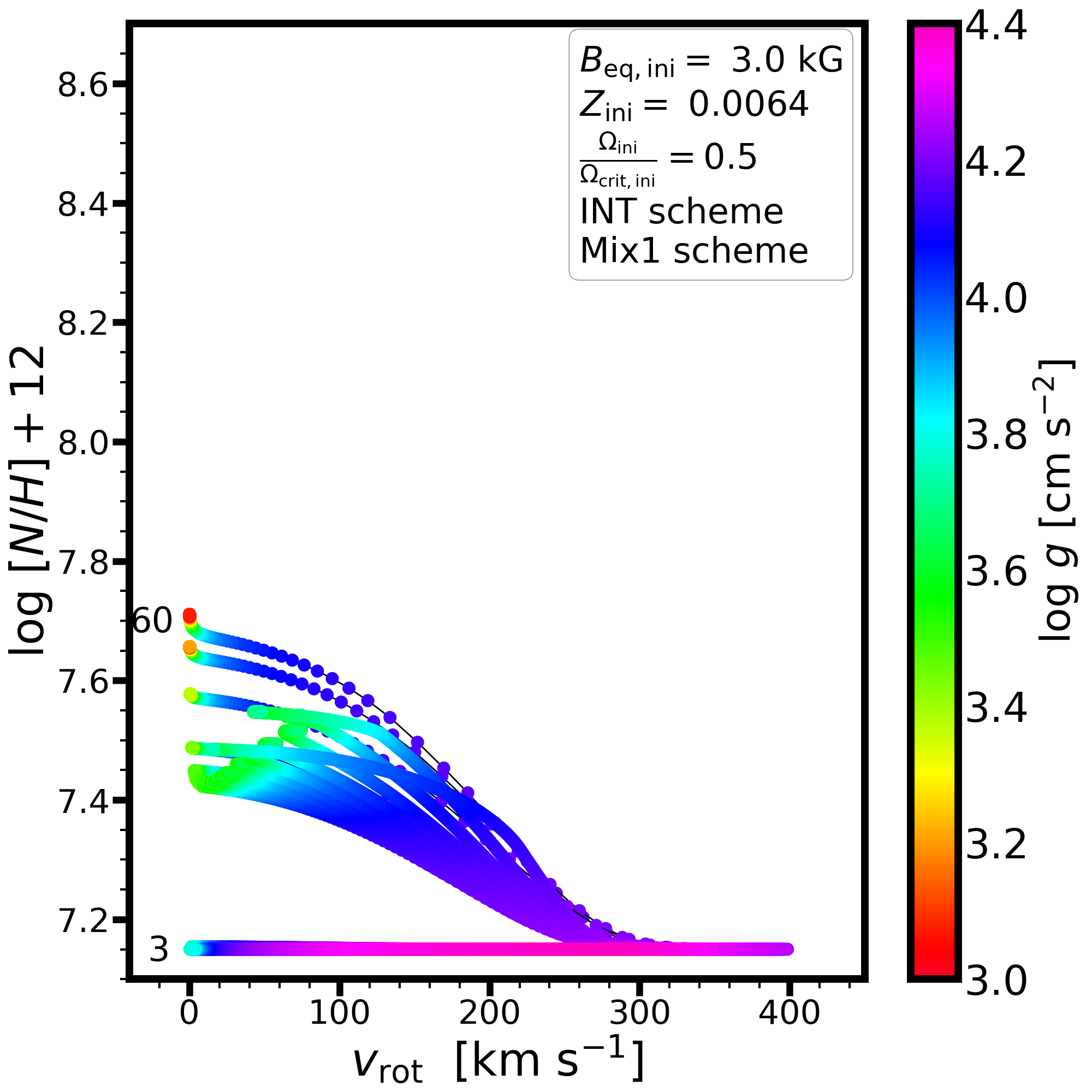
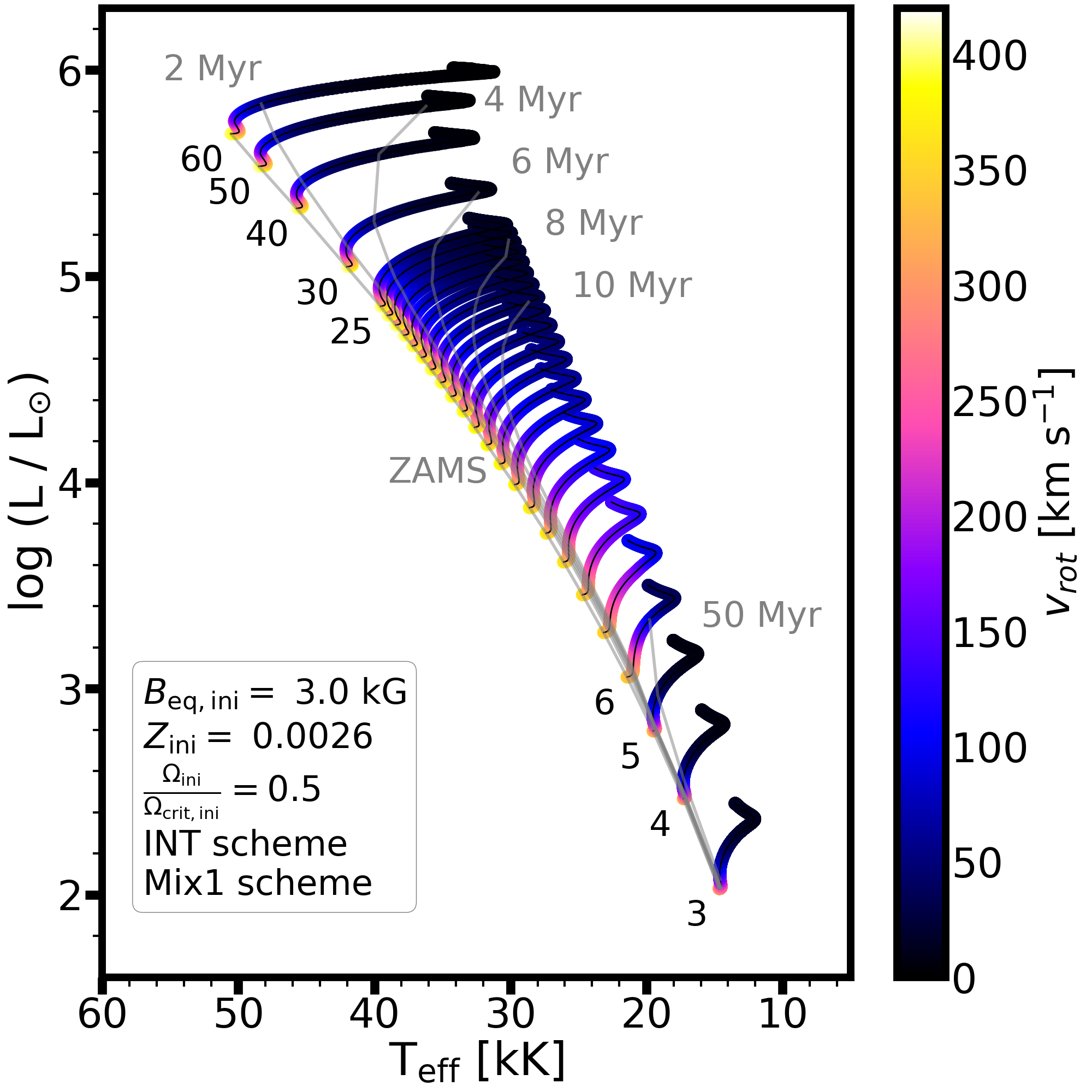
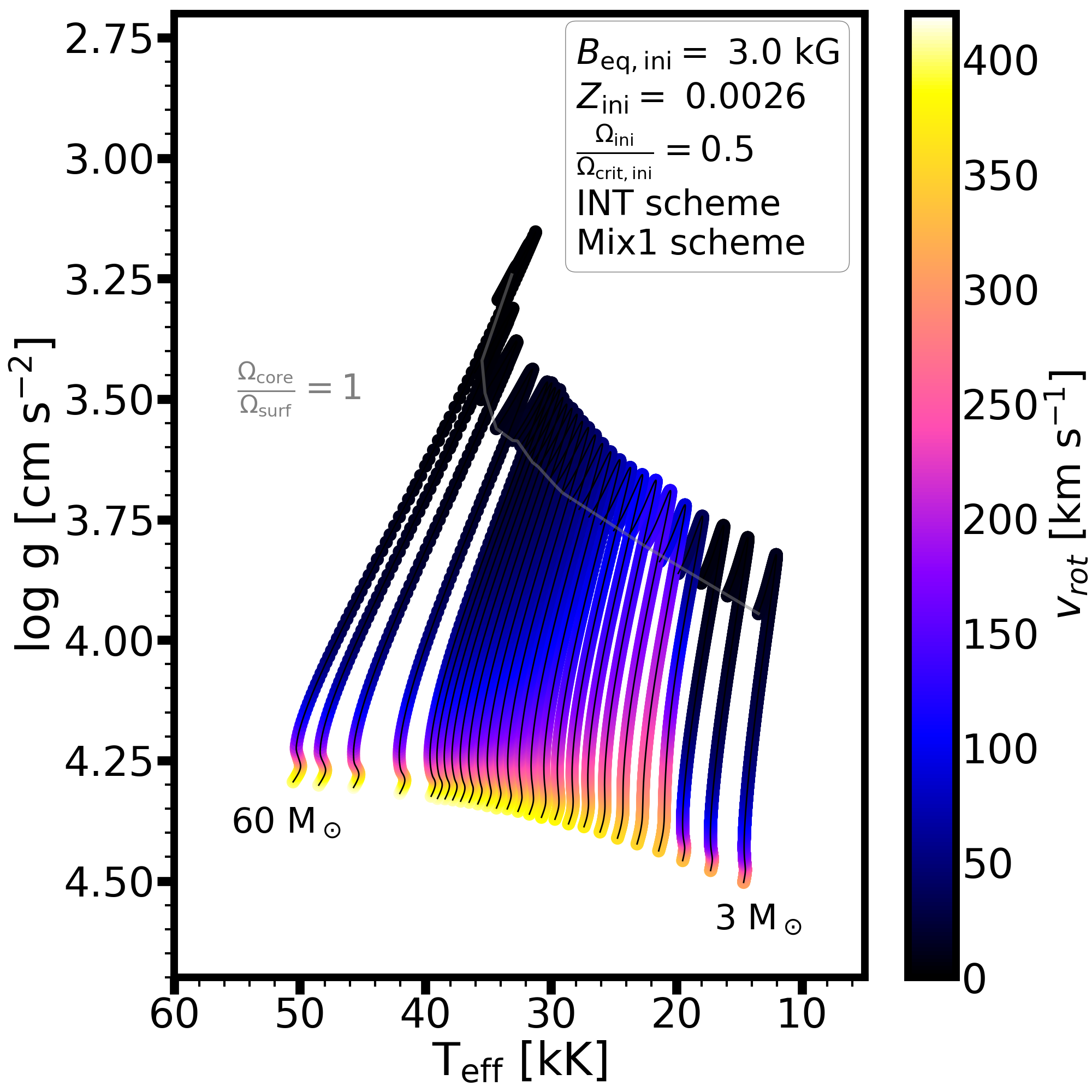
Figure 10: Same as Figure 9 but varying the metallicity (upper - LMC, lower - SMC), within the INT/Mix1 scheme for an initial equatorial magnetic field strength of 3 kG.

3.2.6 Impact of metallicity

Figure 10 shows the impact of the initial metallicity (here, for LMC and SMC values; the Solar metallicity models with the same input are shown in the lower panels of Figure 9) for 3 to 60 M_⊙ models with initial equatorial magnetic field strengths of 3 kG within the INT/Mix1 scheme on the HRD, Kiel, and Hunter diagrams. At lower metallicity, the ZAMS is shifted to higher effective temperatures given that the stellar models are more compact due to the lower opacity and lower mean molecular weight. Specifically, the lower CNO abundances impose further contraction of a star to initiate core burning.

Magnetic braking, in our formalism, is metallicity independent. However, rotational mixing is not. The various mixing prescriptions depend on chemical composition and their gradients, which in turn affects the evolution of surface rotational velocity as most prominently revealed on the Kiel diagrams. For example, for a given value of a diffusion coefficient, the mixing timescale is $\tau\approx R^{2}/D_{\rm chem}$. Since stars are more compact in lower $Z$, the timescale becomes shorter. Consequently, the changes in rotation and surface abundances can be more impacted in lower metallicity stars.

Similarly, the highest relative nitrogen enrichment is seen when metallicity is the lowest (see also e.g. Brott et al. 2011a; Georgy et al. 2013). Let us recall that Figure 10 shows the INT/Mix1 models, which – in our approach – are the lowest estimates for the surface enrichment (c.f. Figure 6). The other schemes predict higher surface nitrogen enrichment when combining the effects with low metallicity. The trends produced in magnetic massive star models are unique since they lead to simultaneous surface nitrogen enrichment and a rapid spin-down of the stellar surface (c.f. Paper I, Paper II). The rapid spin-down could otherwise only be expected for very massive stars with extremely strong stellar winds.

4 Discussion

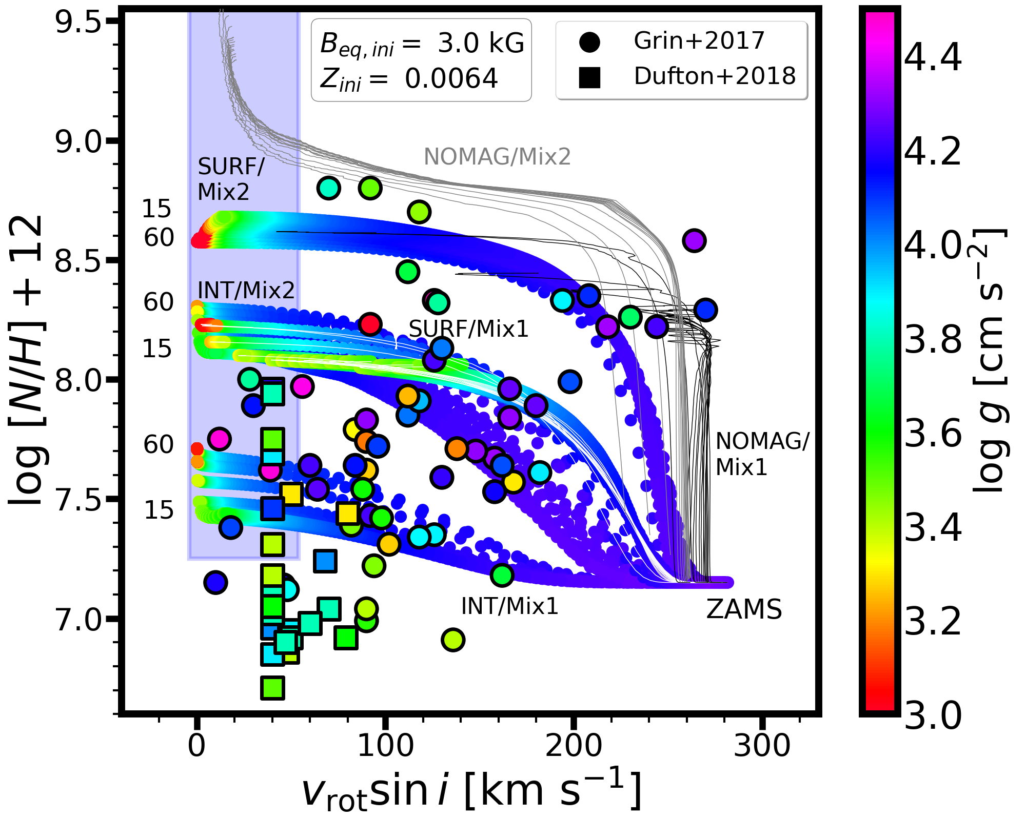
Figure 11: Hunter diagram of magnetic single-star evolutionary models with $B_{\rm eq,ini}=3$ kG, $\Omega_{\rm ini}/\Omega_{\rm ini,crit}=0.5$ at LMC ($Z_{\rm ini}=0.0064$) metallicity within the four schemes. Models within the SURF/Mix1 scheme are also shown with white lines since they overlap with the INT/Mix2 models. Additionally, two sets of non-magnetic (NOMAG) models are shown within the Mix1 (grey) and Mix2 (black) schemes. For visualisation purposes, we reduced the numerical noise in the latter case. Models with initial masses from 15 to 60 M_⊙ are shown. The actual surface equatorial rotational velocity of the models is scaled by $\sin(\pi/4)$ to account for an average inclination angle. The coloured area corresponds to our definition of Group 2 stars. The colour-coding of the models shows the logarithmic surface gravity. Observations are shown with circles and squares, respectively. A typical reported uncertainty in the observed nitrogen abundances is about 0.1 dex.

4.1 Slowly-rotating nitrogen enriched stars in the LMC

The projected rotational velocities of massive stars in the Magellanic Clouds appear to follow a bi-modal distribution (e.g., Dufton et al., 2013, 2018; Dufton et al., 2019, 2020; Rivero González et al., 2012; Ramírez-Agudelo et al., 2013, 2015). The bi-modality is also observed for intermediate-mass stars up to about 5 M_⊙ (e.g., Bastian et al., 2020; Sun et al., 2021). The observed slowly-rotating red main sequence stars and rapidly-rotating blue main sequence stars are thought to be evidence for main sequence splitting (e.g., Bastian et al., 2020) and an extended main sequence turn-off (e.g., D’Antona et al., 2015). It has been suggested that the low-velocity peak might be caused by magnetic braking (e.g., Wolff et al., 1982; Sun et al., 2021). Shultz et al. (2018) demonstrated that the dichotomy in $v\sin i$ between Galactic B-type stars with and without magnetic fields is at least qualitatively consistent with the lower $v\sin i$ values observed in the magnetic population. For observed massive stars in the Magellanic Clouds, a notable fraction of slow-rotators were found to show measurable nitrogen enrichment, which challenges typical, non-magnetic single-star evolutionary models Lennon et al. (1996); Lennon et al. (2003); Dufton et al. (2006); Dufton et al. (2013, 2018); Dufton et al. (2019, 2020); Rivero González et al. (2012); Ramírez-Agudelo et al. (2013, 2015); McEvoy et al. (2015); Grin et al. (2017).

The nitrogen-enriched slow-rotators (also known as "Group 2" stars, Hunter et al. 2008) correspond to roughly 20% of the population in the LMC (e.g., Hunter et al., 2008; Brott et al., 2011b; Grin et al., 2017; Dufton et al., 2018). In the Galaxy, the observed incidence rate of fossil magnetism is found to be $\approx 10\%$ (e.g., Fossati et al., 2016; Grunhut et al., 2017; Sikora et al., 2019a) and it has previously been suggested that at least some of the Group 2 stars could be explained by magnetism (Meynet et al. 2011; Potter et al. 2012b, Paper I). This would require an incidence rate of fossil magnetism in the LMC that is likely higher than the 10% observed in the Galaxy. In addition, the (initial) magnetic field strength distribution is not yet known in our galaxy or in other metallicity environments; however, see Petit et al. (2019) and Cerrahoğlu et al. (2020) for theoretical models. It could also be that the Group 2 stars require an additional channel to explain all observations. In fact, binarity has been suggested by, e.g., Song et al. (2018b).

Figure 11 shows the Hunter diagram with models representative of LMC metallicity ($Z=0.0064$). Let us recall that we specifically adopted an initial nitrogen abundance in our models of $\log(N/H)+12=7.15$ from Dopita et al. (2019) to produce evolutionary models guided by available empirical baseline abundance determinations. Here we demonstrate some of the complex parameter-space dependences that magnetic single-star models produce, albeit strongly depending on the model assumptions, especially the mixing and braking schemes (see also Meynet et al. 2011; Potter et al. 2012b, Paper I, Paper III). We display the non-magnetic models as well as magnetic models in the two braking and two mixing schemes. The initial equatorial magnetic field strength is 3 kG and the initial rotation is set by $\Omega_{\rm ini}/\Omega_{\rm ini,crit}=0.5$. These assumptions produce evolutionary models, which over time reasonably approximate mean values measured from observations (magnetic field strengths from, e.g., Shultz et al. 2018 for Galactic magnetic B-type stars, and rotational velocities from, e.g., Dufton et al. 2013 for massive stars in the Magellanic Clouds). For example, the 3 kG initial ZAMS magnetic field strength weakens by roughly an order of magnitude (since $B_{\rm eq}\propto R_{\star}^{-2}$ over time) at the TAMS to 300 G. Only models with initial masses from 15 to 60 M_⊙ are shown given that the available instrumentation allows magnitude limited observation of bright LMC stars that are more massive than $\approx$ 15 M_⊙ (e.g., Schneider et al., 2018). Thus the models are the most representative of O (and early B-type) stars.

Non-magnetic models (black and grey lines for the Mix1 and Mix2 schemes, respectively) mostly show high rotational velocities. Close to the TAMS, the NOMAG/Mix2 models spin down efficiently and yield a high N/H ratio. However, this prediction is associated with producing Helium stars since these models experience Wolf-Rayet type mass loss due to their quasi-chemically homogeneous main sequence evolution (see Section 15). This helps to decrease the surface hydrogen abundance significantly, and hence the N/H ratio can further increase. Given the high effective temperatures that these models show close to the TMAS, we do not expect that the non-magnetic models should match the observations of typical Group 2 stars.

Chemical mixing remains challenging to constrain. The schemes that we assume in this work cover a large area on the Hunter diagram, which represents modelling uncertainties. In our models, for a given initial rotation and initial magnetic field strength, the INT/Mix1 and SURF/Mix2 models lead to the smallest and highest amount of nitrogen enrichment, respectively (see also Figure 6). The INT/Mix2 and SURF/Mix1 models produce similar results, although the latter models cover a narrower domain. In this sense, the Mix1 and Mix2 schemes are limiting cases in terms of the produced nitrogen enrichment from our models. In nature, the situation might be much more complex since, for example, the study of slowly-pulsating B-type stars reveals a diverse range of mixing profiles (Pedersen et al., 2021). The variation of these profiles over time is not yet quantified.

The magnetic properties of stars in the LMC remain unknown. For this reason, the INT and SURF braking schemes represent assumptions and uncertainties that could only be resolved if, at least, upper limits on the magnetic field strengths were constrained. From the models we see that for a given initial magnetic field strength, the INT models produce less enrichment than the SURF models in a given mixing scheme.

In Figure 11 we show abundance measurements of observed massive stars at the LMC made by Grin et al. (2017) and Dufton et al. (2018). Since the observations only allow derivation of the projected rotational velocity $v~{}\sin~{}i$, we scale the actual rotational velocity in our models with $\sin(\pi/4)$ to account for an average inclination angle. We only consider here observations with $v\sin i<300$ km s^-1.

The observations reveal a large scatter, which likely represents a range of initial conditions (mass, rotation rates, magnetic field strength, binarity, etc.) and current age. The data from Grin et al. (2017) and Dufton et al. (2018) indicate stars in their main sequence evolutionary stages with surface gravities systematically decreasing towards lower rotation rates. Our models show that magnetic braking typically yields slowly-rotating stars early on in the evolution, still with high surface gravities. Once the rotation is slow (and $\log g$ is still $\approx$ 4.0), chemical mixing becomes inefficient and no further surface enrichment may be expected on the main sequence. This is the primary reason why magnetic models produce less surface enrichment than non-magnetic models with the same mixing assumptions (see also Figure 18). However, at this point, the magnetic models still evolve further in time, albeit their location does not change in the Hunter diagram. Thus the magnetic models decrease their surface gravities (to $\log g\approx$ 3.0) in a narrow region in the Hunter diagram, when their (assumed projected) surface rotational velocities are below 50 km s^-1 in all cases, except for the SURF/Mix1 models where the spin-down is the least efficient (c.f. Section 3.2.1).

There are several other caveats, which hamper a quantitative comparison between the models and observations. For example, the mass determinations are uncertain and often rely on (non-magnetic) evolutionary models. As we demonstrate in Figure 11, even for an idealised situation where the braking and mixing schemes were known for a given magnetic field strength, the produced nitrogen enrichment is still a function of initial mass (see also Aerts et al. 2014; Maeder et al. 2014). In the INT/Mix1 scheme, the final nitrogen abundance becomes a factor of 2.5 higher when increasing the stellar mass from 15 to 60 M_⊙. This difference is less in the INT/Mix2 and SURF/Mix1 schemes (factor of $\approx$1.5), while this trend reverses for the SURF/Mix2 scheme.

Despite all these uncertainties, the models incorporating the effects of surface fossil magnetic fields can cover the region on the Hunter diagram where the "anomalous" Group 2 stars (slow rotation along with surface nitrogen enrichment, see Hunter et al. 2008) are located, which is not possible with standard main sequence evolutionary models of single stars (see Martins et al. 2017 for non-magnetic $\approx$ 30 M_⊙ models in the Galaxy). In particular, for the slowly-rotating non-magnetic Mix2 models the produced nitrogen enrichment seems to be larger than indicated by observations, whereas the non-magnetic Mix1 models do not spin down sufficiently.

Since the parameter space is degenerate, not only the mixing and braking scheme could produce results that cover Group 2 stars but also the variation of initial magnetic field strength in a given scheme. A stronger initial field would yield less enrichment (Figure 9), possibly explaining the less nitrogen enriched stars, whereas a weaker initial field could be compatible with the most highly enriched stars (see Figure 18). To quantify this, we introduce and discuss the cutoff magnetic field strength in the next section.

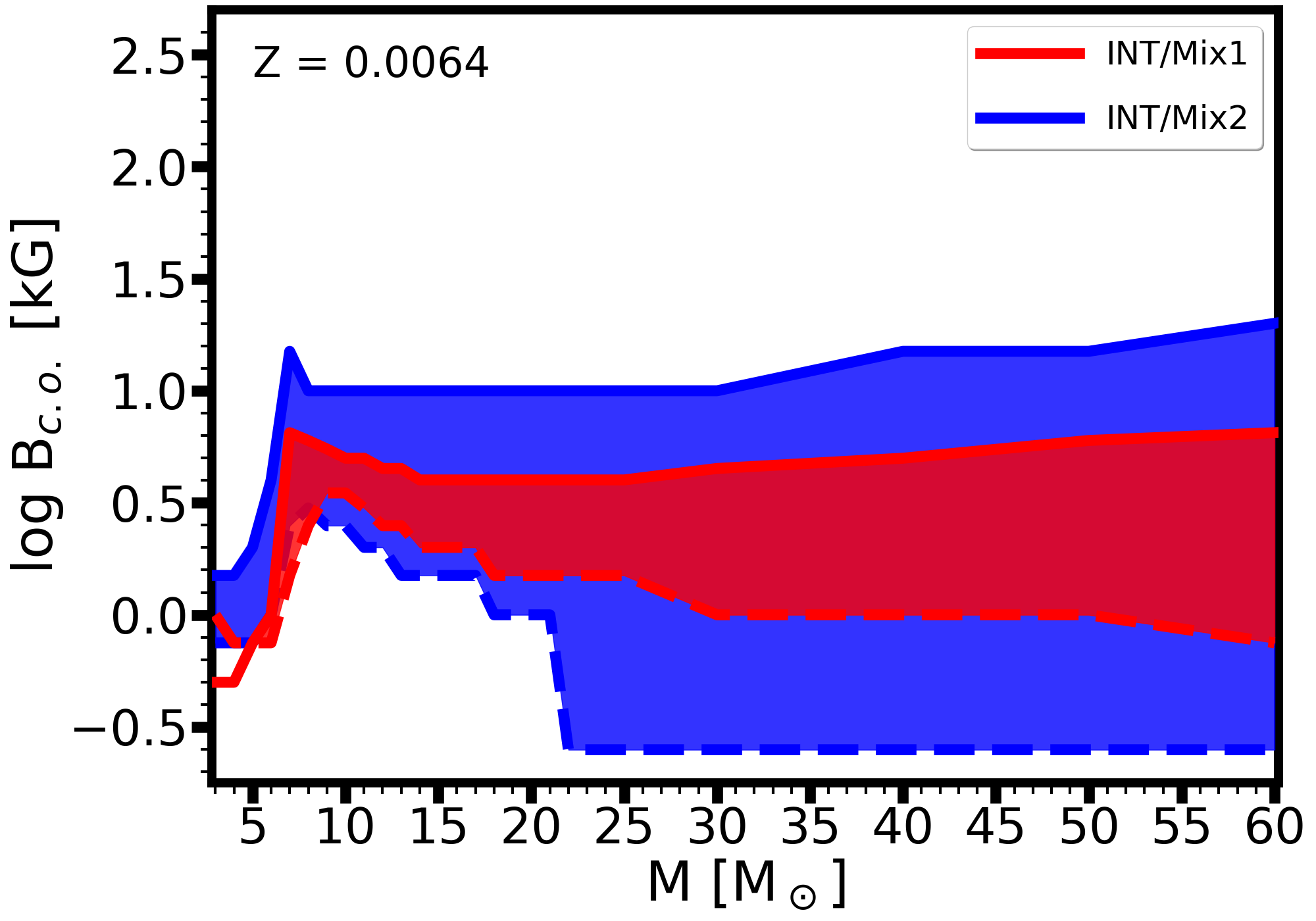
Figure 12: Cutoff magnetic field strengths as a function of mass to produce surface nitrogen enrichment ($B_{\rm max,N}$, solid line) and slow rotation ($B_{\rm min,v}$, dashed line). Values above $B_{\rm max,N}$ will inhibit surface nitrogen enrichment, whereas values below $B_{\rm min,v}$ will not spin down the star sufficiently. Left/right panels show the INT/SURF models. The models are considered for initially $\Omega/\Omega_{\rm crit}=0.5$ at LMC ($Z=0.0064$) metallicity.

4.2 Cutoff magnetic field strengths in the LMC

It is of interest to evaluate a critical value of the magnetic field that strongly impacts observable properties. In particular, what range of initial magnetic field strengths allow for producing Group 2 stars? To this extent, we define a cutoff (maximum) field strength $B_{\rm max,N}$ as the initial equatorial magnetic field strength in a given model that allows for producing more than 0.1 dex of surface nitrogen enrichment (in spectroscopic units) during its main sequence evolution. If the initial magnetic field strength is higher than $B_{\rm max,N}$, then the mixing is inefficient due to the magnetic spin-down, and no nitrogen enrichment can be observed. Similar to the above definition, we may also define a cutoff (minimum) magnetic field strength that is the initial equatorial magnetic field strength needed to produce sufficiently slow rotators ($v_{\rm rot}<71$ km s^-1) by the end of the main sequence evolution. Any value higher than $B_{\rm min,v}$ will yield slow-rotating models; however, values below $B_{\rm min,v}$ will still result in considerable rotational velocities at the TAMS. Figure 12 shows the range of possible initial equatorial magnetic field strengths that are able to produce Group 2 stars given the constraints given above. $B_{\rm max,N}$ is shown with solid line and $B_{\rm min,v}$ with dashed line. The range is shown as a function of initial mass for the LMC (the Solar and SMC metallicity models are discussed in Appendix F). The cutoff field strengths depend on the initial rotation rates, metallicity, mass, and chemical mixing and magnetic braking schemes. We discuss now the latter three.

Models within the INT/Mix1 scheme result in the lowest value of $B_{\rm max,N}$ since this scheme is the least efficient in chemical mixing. However, stronger magnetic fields would brake the rotation faster than the timescale of rotational mixing. In contrast, models within the SURF/Mix2 scheme have such strong mixing that even a 50 kG equatorial field strength is insufficient to inhibit mixing. A particular feature, a jump in $B_{\rm min,v}$ around 5 to 10 M_⊙, can be explained by the mass-dependent rotational behaviour of the models discussed in Section 3.2.4. In most models, the decreasing value of $B_{\rm min,v}$ for stars more massive than 10 M_⊙ implies that stronger stellar winds aid the spin-down thus a weaker magnetic field is sufficient to achieve slow-rotating stars.

We find that equatorial magnetic fields of initially a few kG are able to produce Group 2 stars in the INT/Mix1 scheme. Nevertheless, the range of allowed initial field strengths is the most limited in this case. In fact, models below 6 M_⊙ are in a "forbidden" range where the minimum field strengths needed to brake rotation are higher than the maximum field strengths allowed to produce nitrogen enrichment. In the INT/Mix2 scheme, a much larger range of initial field strengths are allowed to produce Group 2 stars, particularly from 22 M_⊙, where the lower limit drops to 250 G. For initial masses higher than 7 M_⊙, the upper limit is of the order of 10 kG to produce Group 2 stars.

Models within the SURF/Mix1 and SURF/Mix2 schemes (right panel of Figure 12) cover a wide range of possible initial field strengths. The SURF/Mix1 scheme produces a similar mass-dependent pattern as the models in the INT scheme. Namely, models from 10 M_⊙ have systematically decreasing values of $B_{\rm min,v}$. However, for initial masses lower than 17 M_⊙ a 10 kG initial equatorial field strength is still needed to achieve slow rotation. Interestingly, for initial masses $\geq$ 19 M_⊙ there is a dip in $B_{\rm max,N}$, staying constant at 30 kG in contrast to the mass range of 7-18 M_⊙, where the 50 kG initial equatorial field strength still allows for producing nitrogen enrichment. The SURF/Mix2 models have a constant upper limit given by $B_{\rm max,N}$, meaning that even the strongest initial magnetic field strength we considered in this study is not sufficient to prevent nitrogen enrichment on the main sequence. The lower limit given by $B_{\rm min,v}$ is constant for initial masses higher than 6 M_⊙. In general, we can conclude that the INT scheme favours lower values for the cutoff magnetic field strengths of $B_{\rm max,N}$ to produce Group 2 stars and the SURF scheme allows for higher values of $B_{\rm max,N}$. It is quite remarkable that the upper limit remains roughly constant in the INT cases for stars more massive than about 10 M_⊙. In the SURF/Mix2 case, likely an unrealistically strong magnetic field would be needed to prevent nitrogen enrichment (as the 50 kG field is still insufficient). The Mix1 scheme tends to allow for a narrow range of values and Mix2 scheme covers a wide range of possible solutions.

In the LMC, both quantities used in our criteria, surface nitrogen abundance and (projected) rotational velocity, can be measured. Large-scale surveys dedicated to magnetic field measurements are not yet available in lack of high-resolution spectropolarimetry (however, see Bagnulo et al. 2017, 2020). This means that our predictions can be used as constraints on the strengths of magnetic fields that might exist in slowly-rotating nitrogen-enriched ("Group 2") stars in the Magellanic Clouds. An initial equatorial magnetic field strength above $B_{\rm min,v}$ and below $B_{\rm max,N}$ will produce stars that can be identified as Group 2 stars.

4.3 Future work

The models presented in this work cover the main sequence phase of single stars. Logical extensions include calculating pre-main sequence models and continuing the computations to the post-main sequence phase to be able to scrutinise connections with end-products of stellar evolution, such as strongly magnetised white dwarfs and neutron stars (magnetars). The recently discovered link between magnetars and fast-radio bursts (CHIME/FRB Collaboration et al., 2020; Bochenek et al., 2020) further supports investigations of the magnetic field origin of magnetars (e.g., Spruit, 2009; Makarenko et al., 2021). Our grid of models could be further extended to cover initial masses below 3 M_⊙ and thus to compare with, for example, Ap stars. This requires some further considerations about the winds of these objects and the inclusion of atomic diffusion in the models. We assumed single-star models in this work. Some magnetic massive stars, such as $\tau$ Sco (Schneider et al., 2016; Schneider et al., 2019; Schneider et al., 2020; Keszthelyi et al., 2021), may challenge this scenario. Nonetheless, the vast majority of OBA stars with fossil fields have characteristics that do not require invoking a merger event. In particular, fossil magnetic fields are detected in young massive stars, for example, in $\sigma$ Ori E (Landstreet & Borra, 1978; Townsend et al., 2010; Oksala et al., 2012; Song et al., 2021). Certain binary systems also present challenges to the merger scenario, such as the doubly-magnetic binary $\epsilon$ Lupi (Shultz et al., 2015) and the eclipsing late B-type binary HD 62658, which comprises two young nearly-identical stars in a circularised orbit, only one of which is magnetic (Shultz et al., 2019c). Thus single-star models presented in this work are a reasonable first approach; however, future work remains to address binarity and mergers in combination with fossil field effects. In particular, multiplicity is common among massive stars (Sana et al., 2012, 2014; de Mink et al., 2013, 2014) and while close magnetic binary systems are rare (e.g., Alecian et al., 2013; Shultz et al., 2018), the mutual impact of magnetism and tidal interactions need to be further studied (e.g., Song et al., 2018a; Vidal et al., 2018).

The models computed in this work can be confronted with observations of known magnetic massive stars. They will complement previous approaches which relied on grids of stellar evolution models that did not include surface magnetic field effects (e.g., Brott et al., 2011a; Ekström et al., 2012; Chieffi & Limongi, 2013; Choi et al., 2016) to infer stellar parameters and ages of magnetic stars. The differences are expected to be most pronounced for higher-mass stars (Petit et al., 2017), whereas – within the framework considered here – the lower-mass, A-type stars should be less impacted (Deal et al., 2021). Nonetheless, the available TESS data and continuous spectropolarimetric monitoring can be used to constrain accurate rotation periods of such stars and directly compare with evolutionary models incorporating magnetic braking.

The INT models represent stars with strong, predominantly dipolar fields that are commonly identified in the sample of known magnetic massive stars. The SURF models are a limiting case motivated by stars with complex magnetic fields. In the future, the implementation of different magnetic field configurations and their time evolution could be considered to improve the present models.

The internal mixing efficiency remains uncertain in evolutionary modelling. In our models, quasi-chemically homogeneous evolution during the main sequence develops in the non-magnetic Mix2 case. In the INT/Mix2 models this behaviour is prevented by the efficient overall spin-down already when initially weak magnetic fields are considered, whereas in the SURF/Mix2 models a very efficient mixing still remains. The occurrence and duration of quasi-chemical evolution depends on the initial field strength and stellar mass; some SURF/Mix2 models evolve significantly bluewards, whereas some models turn to a redward evolution after mixing becomes less efficient (see Figure 17). Quasi-chemically homogeneous evolution is expected to be rare in nature; however, it may be a crucial channel, for example, for some supernova events, gamma-ray bursts, or gravitational wave sources (e.g., Georgy et al., 2012; Martins et al., 2013; de Mink & Mandel, 2016; Szécsi, 2017).

Observational studies should help constrain the mixing efficiency and ultimately the physical mixing processes. As such, it would be beneficial to further study our models and confront them with measurements of surface nitrogen abundances in magnetic massive stars (Morel et al., 2008, 2015; Aerts et al., 2014; Martins et al., 2012; Martins et al., 2015), as well as studies which identified anomalous trends on the Hunter diagram in the LMC and SMC (e.g., Dufton et al., 2020, and see Section 4.1).

Finally, our current understanding of magnetic field evolution is still incomplete and, in particular, how different field geometries evolve over time is largely unconstrained. It will therefore be valuable to explore various field evolution scenarios, for example, magnetic flux decay (Shultz et al. 2019b, Paper III). This might also lead to a time-dependent magnetic braking scheme depending on the relative dissipation timescales of various complex field components.

5 Conclusions

In this work we present the most extensive grid of stellar structure and evolution models taking into account the effects of surface fossil magnetic fields. The grid is publicly available on Zenodo and we recommend that, while acknowledging the uncertainties, it could be used to infer stellar parameters of known magnetic massive stars. No particular braking (INT/SURF) or mixing (Mix1/Mix2) scheme can be preferred at this time, although we do assume that if the field geometry is known, the INT case is applicable for dipolar fields and the SURF case for more complex geometries. Thus we consider the four schemes as limiting cases and, as we demonstrate in this work, the differences between these subgrids can substantially impact the determination of stellar parameters. It is therefore essential to confront the Mix1/Mix2 mixing schemes with spectroscopic studies even for stars where surface magnetic fields are not detected. In all cases (2 mixing schemes and 3 metallicities), we provide a subgrid of non-magnetic evolutionary models. Furthermore, the grid of models is suitable for population synthesis studies, which thus far have neglected magnetic field effects and magnetic massive stars within stellar populations (however, see Potter et al., 2012b). The impact of magnetic fields nonetheless may have important consequences on stellar populations and stellar-end products, for example, considering progenitors of magnetars (e.g., Schneider et al., 2019).

We demonstrate that magnetic braking by a fossil field leads to efficient spin-down. For example, an initial equatorial field of 3 kG strength at solar metallicity is sufficient in most models to decrease an initial surface equatorial rotational velocity of 300 km s^-1 below 50 km s^-1 within the early stages of the main sequence evolution (e.g., Figure 8). For a given magnetic field strength, the spin-down of high-mass stars (> 10 M_⊙) is further aided by mass-loss, whereas the spin-down of lower-mass stars in our grid (< 5 M_⊙) is identifiable due to the long nuclear timescale. The intermediate-mass range (5-10 M_⊙) has the least efficient spin-down over the main sequence evolution.

The "magnetic population" is thus far only identified within the Galaxy by spectropolarimetry and it is unknown what fraction of massive stars possesses strong, surface magnetic fields in extragalactic environments. Generally, the spin-down of the stellar surface for a given magnetic field strength is the most rapid at high metallicity (due to stronger winds), whereas the measurable surface nitrogen abundances are more impacted at lower metallicity (as chemical mixing effects are more pronounced). In the Large Magellanic Cloud, about 20% of stars follow an anomalous pattern on the Hunter diagram, which can be covered with magnetic stellar evolution models. We identify the existence of a range of initial magnetic field strengths (the exact values depending on metallicity, mixing schemes, etc.) that allow for producing slowly-rotating nitrogen enriched Group 2 stars. The lower limit is constrained by a field strength that is needed to brake rotation and produce slow rotators. The upper limit is constrained by a field strength that is needed to allow for rotational mixing and still produce nitrogen enrichment. The range of possible field strengths for the INT models is much narrower than for the SURF models, however, it is compatible with typically measured values. In the LMC and SMC almost all (except some of the lowest mass) models lead to a solution. Contrary, we find that in the Galaxy the formation of Group 2 stars may essentially be prevented for initial masses from 6 to 23 M_⊙ in the INT/Mix1 scheme (Figure 31).

Overall, we find significant differences between the braking and mixing schemes. With internal magnetic braking caused by a strong dipolar field, differential rotation cannot develop. With surface magnetic braking caused by a complex magnetic field the physical scenario remains much less clear; the results strongly depend on the chosen assumptions regarding chemical mixing.

Data Availability

A full reproduction package is available on Zenodo at https://doi.org/10.5281/zenodo.7069766, in accordance with the Research Data Management Plan of the Anton Pannekoek Institute for Astronomy at the University of Amsterdam.

The data used in this paper amounts to the order of 1/3 TB. A typical evolutionary model ("history" file in mesa nomenclature) is a few MBs, whereas a typical structure model ("profile" file in mesa nomenclature) is 10 MB. Each evolutionary model has three structure models saved at the ZAMS, mid-MS, and TAMS, respectively. In addition to the evolutionary and structure files, we save and provide the ".mod" files of each run when available. This allows for continuing the computations on the post-main sequence. We also generated isochrones for each sub-grid, these are included in the Zenodo record.

Given the large range of covered parameter space, the output data in this paper is particularly useful for stellar evolution and population synthesis studies, as well as to compare with observational results of even individual stars. However, we emphasise that when interpreting observational results the modelling assumptions and uncertainties should be considered.

Appendix A mesa microphysics

The MESA EOS is a blend of the OPAL (Rogers & Nayfonov, 2002), SCVH (Saumon et al., 1995), FreeEOS (Irwin, 2004), HELM (Timmes & Swesty, 2000), PC (Potekhin & Chabrier, 2010), and Skye (Jermyn et al., 2021) EOSes.

Radiative opacities are primarily from OPAL (Iglesias & Rogers, 1993, 1996), with low-temperature data from Ferguson et al. (2005) and the high-temperature, Compton-scattering dominated regime by Poutanen (2017). Electron conduction opacities are from Cassisi et al. (2007).

Nuclear reaction rates are from JINA REACLIB (Cyburt et al., 2010), NACRE (Angulo et al., 1999) and additional tabulated weak reaction rates; Fuller et al. (1985); Oda et al. (1994); Langanke & Martínez-Pinedo (2000). Screening is included via the prescription of Chugunov et al. (2007). Thermal neutrino loss rates are from Itoh et al. (1996).

Appendix B Mass-loss quenching for quadrupole field geometries

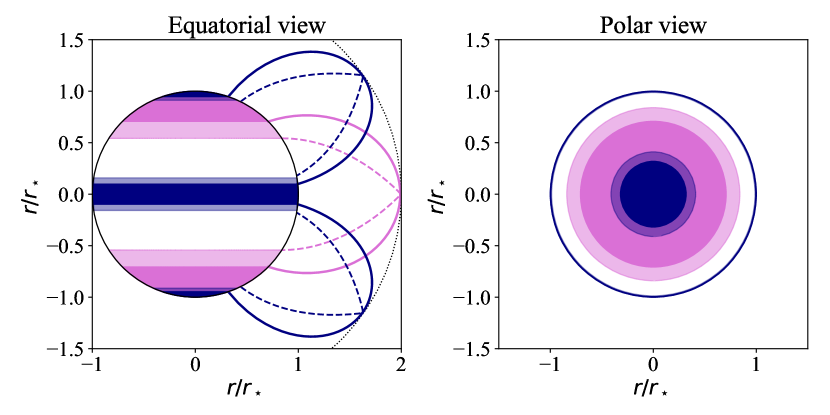
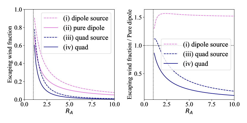
Figure 13: Top: illustration of the surface area covered by open field loops for (i) a dipole extrapolated with a source radius ($2R_{\star}$), (ii) a pure dipole, (iii) a quadrupole extrapolated with a source radius ($2R_{\star}$), and (iv) a pure quadrupole. The radial extent of the largest closed loop is $2R_{\star}$ (grey dotted circle) in all cases. Bottom Left: Escaping wind fraction as a function of closure radius (which is of the order of the Alfvén radius) for the 4 cases above. Bottom right: Same as Left panel, but normalised to the escaping wind fraction of a purely dipolar configuration.

As a simplifying assumption, we consider that even for more complex magnetic fields (represented by the SURF models), a scaling based on the Alfvén radius of a quadrupole field may be adopted to calculate the mass-loss quenching effect via $f_{\rm B}$ (Equations 7-8). Here, we outline the actual geometrical effects of a quadrupolar magnetic field configuration.

Following ud-Doula et al. (2008), the escaping wind fraction is the fraction of the stellar surface covered with open field loops. For a purely dipolar geometry, the region of open field loops corresponds to a polar cap extending from $\mu=1$ to $\mu=\mu_{m}$, where $\mu$ is the cosine of the co-latitude $\theta$, and $\mu_{m}=\cos\theta_{m}$ is the location at which the largest loop connects to the stellar surface (see pink shaded regions in Fig 13).

This assumes that the magnetic field lines retain their pure dipolar geometry, even though in principle the field gets distorted by the outflowing stellar wind. Another approach is to solve for the magnetic field in the magnetosphere using a force-free extrapolation (e.g. Jardine et al., 1999). Assuming that the magnetic field can be expressed as the gradient of a potential $\Phi$ such that $\nabla^{2}\Phi(r,\theta,\varphi)=0$, the magnetic field can be found by imposing a dipolar (or quadrupolar, see below) boundary condition at the surface and imposing that the magnetic field must become radial at a certain distance from the stellar surface (at the so-called source radius, $r_{s}$). Following the description of Gregory (2011) (their Equation 32 with $l=1$), in this case the largest field loops (illustrated in the top left panel of 13 with dashed curves) are connected to the surface at:

$$\sin^{2}\theta_{m}=\frac{1}{r_{m}}\frac{3r_{m}^{3}}{1+2r_{m}^{3}}\,.$$ (23)

For a quadrupolar configuration, open field loops are located in two polar caps ($\mu_{\mathrm{cap}}$) and an equatorial belt ($\mu_{\mathrm{belt}}$) (see 13 top panels in blue shading). Thus the total fractional area of open field lines is:

$$f_{B}=[1-\mu_{\mathrm{cap}}]+[\mu_{\mathrm{belt}}]\,.$$ (24)

For a purely quadrupolar configuration, these footpoints of the largest closed loop can be found by solving for the $\mu_{m}$ roots of:

$$\mu_{m}^{3}-\mu_{m}+\left[\frac{2}{3^{3/2}}\frac{1}{r_{m}^{2}}\right]=0\,,$$ (25)

and for a quadrupole extrapolated with a source radius:

$$\mu_{m}^{3}-\mu_{m}+\left(\frac{1}{r_{m}^{2}}\frac{5r_{m}^{4}}{2+3r_{m}^{4}}\frac{2}{3\sqrt{3}}\right)=0\,.$$ (26)

In general, for the same closure radius the escaping wind fraction (surface covered by open field loops) decreases from extrapolated dipole $\rightarrow$ pure dipole $\rightarrow$ extrapolated quadrupole $\rightarrow$ pure quadrupole. We also recall that for a given field strength the closure radius is smaller for a quadrupole field than for a dipole. The lower panels of Fig 13 display the corresponding change in magnetic mass-loss quenching between the dipolar and quadrupolar geometries as a function of closure radius. In a future work we will implement and study magnetic mass-loss quenching for field geometries that deviate from a pure dipole. As shown here, we expect that a quadrupole field will result in a lower escaping wind fraction, i.e., stronger mass-loss quenching for a given magnetic field strength at a given time. However, the time evolution may sensitively impact the results in the evolutionary context.

Appendix C Convective expulsion and magnetic suppression of convective layers

"Magneto-convection", the interaction between the magnetic field and turbulent motions in convectively unstable stellar layers, has been extensively studied and recent progress warrants a brief discussion of this topic. Modifying Schwarzschild’s criterion for convection, the stability criterion for magneto-convection was first given by Gough & Tayler (1966) and recently revised by MacDonald & Petit (2019), specifically considering radiation pressure to account for sub-surface layers of massive stars, in the form of:

$$Q(\nabla-\nabla_{\rm ad})<\frac{v_{A}^{2}}{v_{A}^{2}+c_{s}^{2}}\left(1+\frac{\mathrm{d}\ln\Gamma_{1}}{\mathrm{d}\ln P}\right)\,,$$ (27)

where $Q$ is the thermal expansion coefficient, $v_{A}$ and $c_{s}$ are the Alfvén and sound speeds, $\Gamma_{1}$ is the first adiabatic exponent, and $P$ is the local pressure. This criterion leads to a critical magnetic field strength, which, if reached, suppresses convection (e.g., Lydon & Sofia, 1995; Feiden & Chaboyer, 2012), whereas, if it is not reached, the field lines are prevented from reconnecting by strong convective turbulence, which over time leads to diffusing the magnetic flux out of those regions (e.g., Parker, 1963). In the one-dimensional stellar evolution models presented in this study, we refrained from using Equation 27. Both MacDonald & Petit (2019) and Jermyn & Cantiello (2020) showed that the key (surface) characteristics during main sequence evolution are not expected to change significantly – when using Equation 27 – for the stellar mass domain considered in this work, except for the 50-60 M_⊙ models. We anticipate that, in general, the post-main sequence evolution needs particular attention due to the structural changes which could lead to the development of extended convection zones.

The cores of main sequence massive stars are strongly convective, such that a critical magnetic field strength, which is needed to suppress convection (according to the stability criterion given in Equation 27) may not be reached. In this case, if the magnetic field strength is below its critical strength throughout the core, it is expected that convection will destroy any large scale, organised magnetic flux. This is commonly known as convective expulsion (Parker, 1963; Weiss, 1966; Spruit, 1979; Tao et al., 1998; Schüssler & Knölker, 2001). While the convective core should expel any fossil magnetic fields, the development of small-scale magnetic fields via convective dynamos (e.g., Stello et al., 2016; Augustson et al., 2016) may lead to a complex physical picture near the core boundary (Featherstone et al., 2009). It is possible that the fossil magnetic field has a strong impact, for example, by suppressing the radiatively unstable overshooting regions (or even the stellar core, to some extent, see, e.g., Petermann et al. 2015). Thus far, magneto-asteroseismology of two magnetic intermediate-mass stars are consistent with a low value of overshooting (Briquet et al., 2012; Buysschaert et al., 2018). This gives some support of using a modest overshooting, at least, in our INT models, where we assume dipoles embedded deep in the stellar radiative zone. However, this question needs to be studied in more detail in a future work.

A domain of interest is the sub-surface layer of massive stars where inefficient convection (accounting for a few percent of the total luminosity transport) is predicted to arise due to the increase in the opacity of iron, known as iron opacity bumps (Cantiello et al., 2009; Cantiello & Braithwaite, 2011; Gräfener et al., 2012). In these radiation-dominated layers, some excess luminosity is transported by convective flux. Using equipartition arguments, Aurière et al. (2007) and Sundqvist et al. (2013) argue that sub-surface convection in radiation-dominated stellar layers can be suppressed by a critical magnetic field when the magnetic pressure reaches the thermal pressure. The exact value of the critical field strength needed to suppress or even inhibit convection remains somewhat uncertain – a problem that is mostly explored for the dynamo fields of low-mass stars (Mullan & MacDonald, 2001; Feiden & Chaboyer, 2012, 2013, 2014; Feiden, 2016; MacDonald & Mullan, 2017). Nevertheless, observations clearly show that the Ap phenomenon disappears for stars less massive than about 1.5 M_⊙, coinciding with the development of efficient convection (due to the hydrogen opacity bump) in the stellar envelope (Landstreet, 1991; Braithwaite & Spruit, 2017). We might therefore assume that extended convective zones cannot develop in regions of massive stars where the fossil field (which reaches the critical strength) permeates through. A fossil magnetic field, observable at the stellar surface, should certainly reach sufficient critical strength in these near-surface layers to inhibit convection. All OB stars show evidence for measurable macroturbulent broadening (Simón-Díaz et al., 2017), including magnetic OB stars (Grunhut et al. 2017; Shultz et al. 2018, with the only exception of NGC 1624-2, see Sundqvist et al. 2013), making them a valuable laboratory to further our understanding regarding the origin of macroturbulence. The observed macroturbulence and the putative lack of subsurface convection in magnetic OB stars would support an origin of macroturbulence (at least, in magnetic stars) that is unrelated to sub-surface convection, and could be due to, for example, wave-propagation from the stellar core (Aerts et al., 2009; Bowman et al., 2020).

Appendix D ZAMS and TAMS stellar structure models

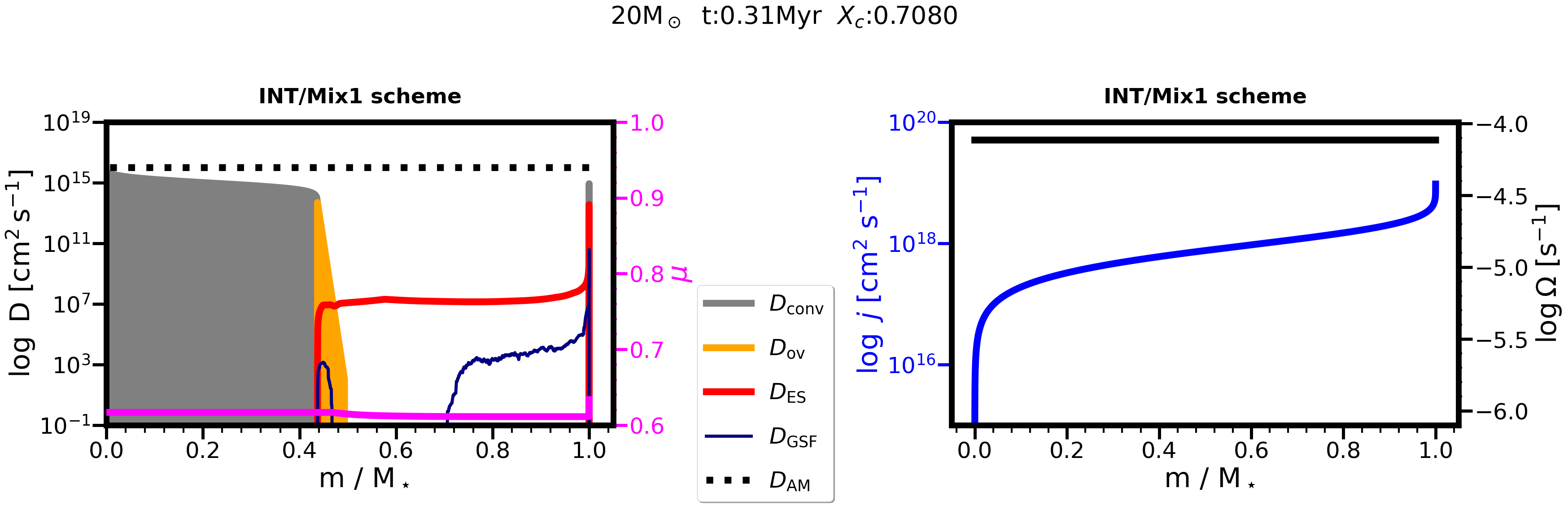
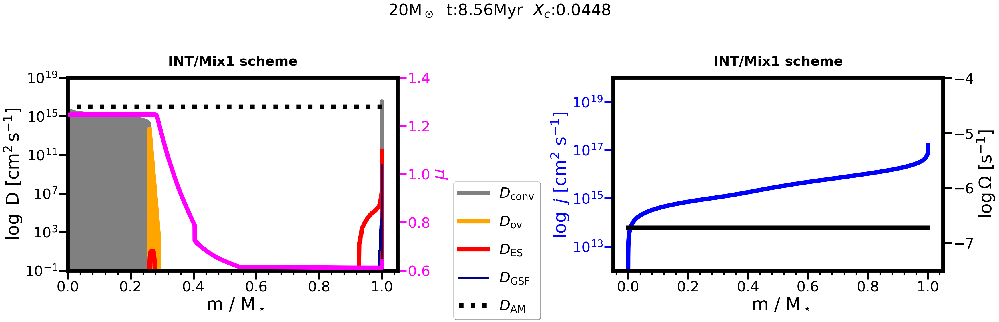
Figure 14: Fiducial model with initial mass of $M_{\rm ini}$ = 20 M_⊙ (and initial equatorial magnetic field strength of 3 kG at $Z=0.014$) in the INT/Mix1 scheme. Left and Right panels are as described in Figure 2. Top: near ZAMS. Bottom: near TAMS.

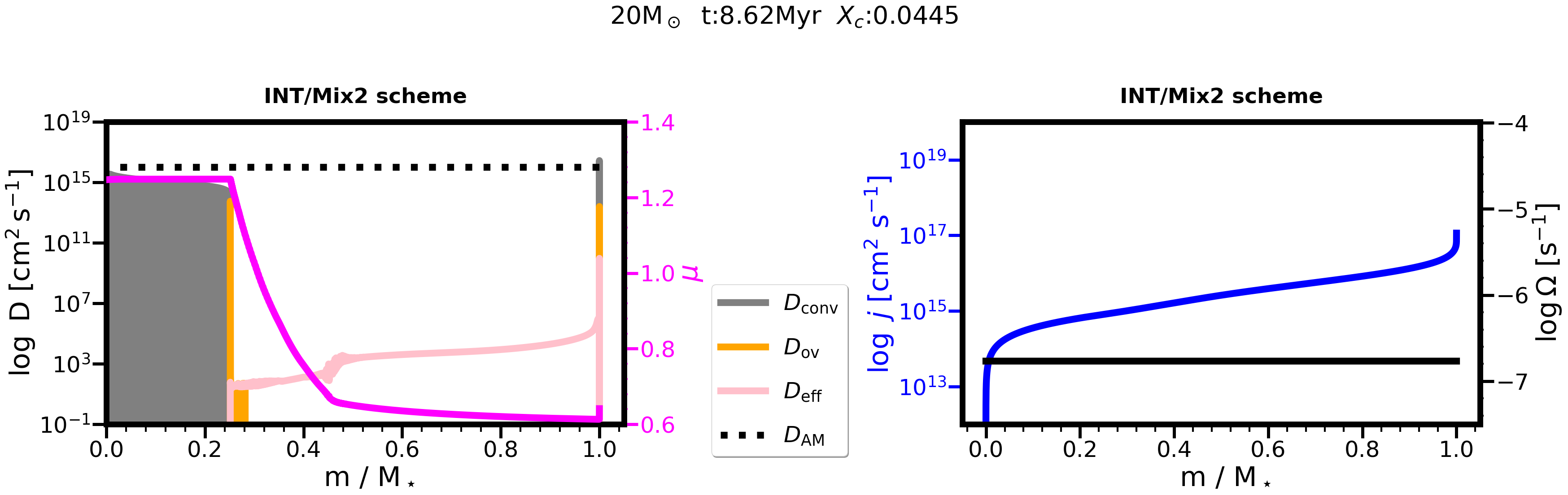
Figure 15: Same as Figure 14 but for the INT/Mix2 scheme.

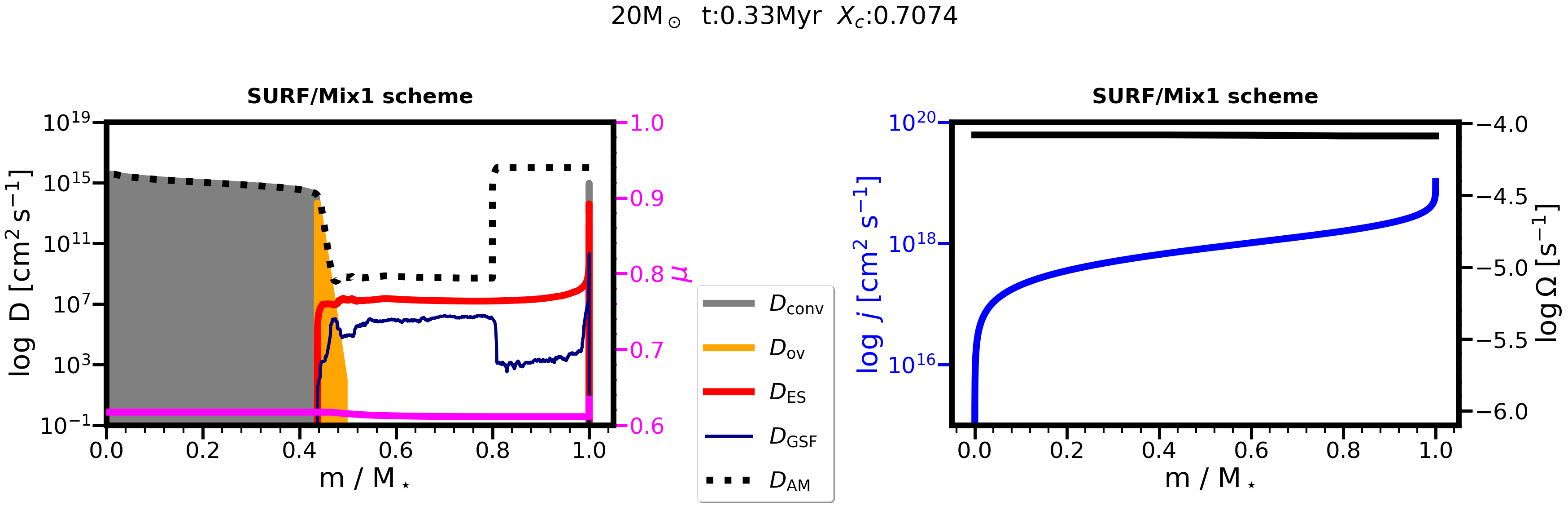
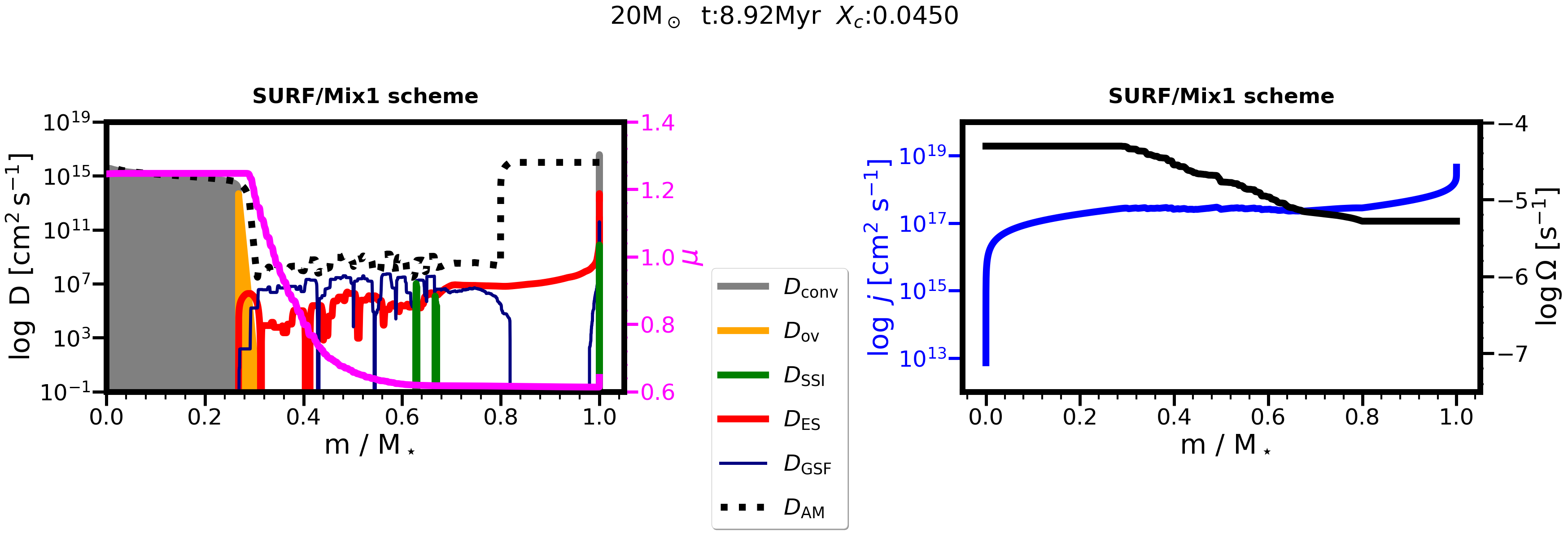
Figure 16: Same as Figure 14 but for the SURF/Mix1 scheme.

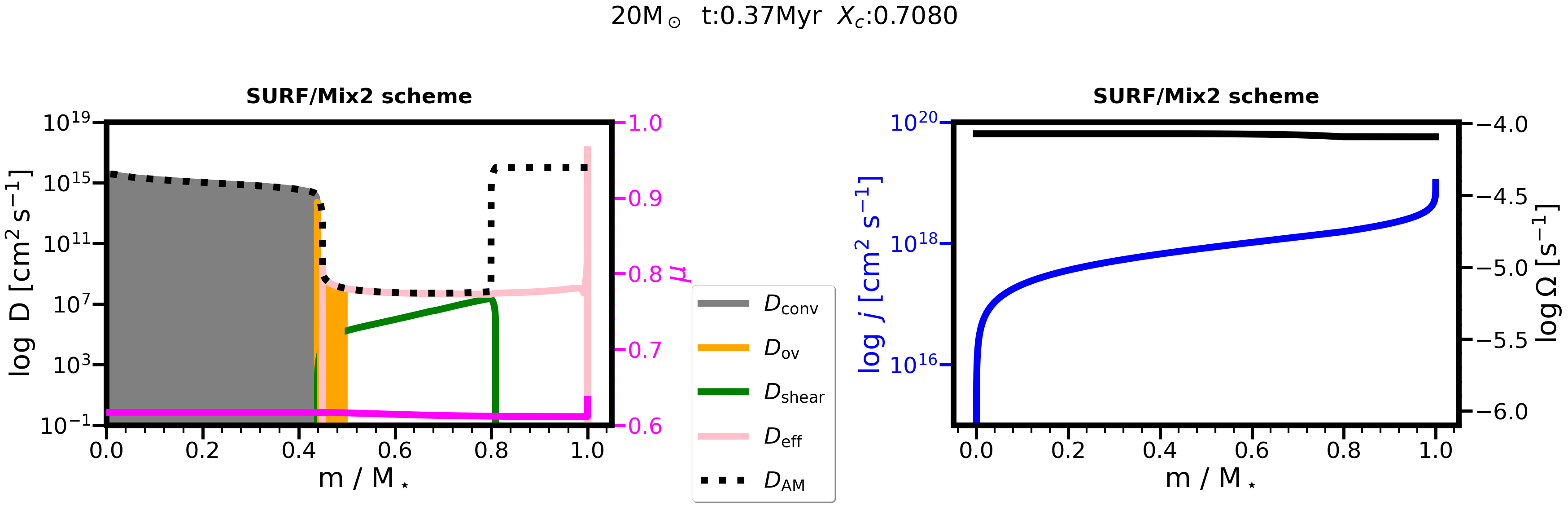
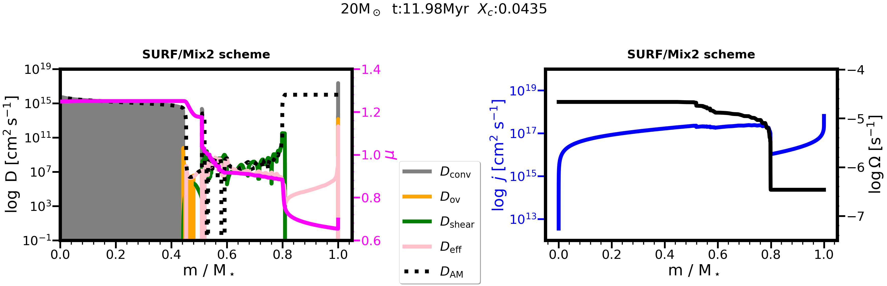
Figure 17: Same as Figure 14 but for the SURF/Mix2 scheme.

Here, we describe the stellar structure models of the fiducial model and the corresponding models with initial masses of 20 M_⊙ in the other braking and mixing schemes at times close to the ZAMS and TAMS. In Figure 14 the INT/Mix1 models are shown. Initially, meridional currents dominate chemical mixing. Given the very efficient magnetic braking in all layers and the solid-body rotation, the angular velocity decreases more than an order of magnitude in all stellar layers from ZAMS to TAMS. Correspondingly, chemical mixing becomes drastically inefficient, leaving a gap between the stellar core and the surface. In Figure 15 the INT/Mix2 models are shown. The results are similar to the INT/Mix1 scheme; however, at the TAMS the effective diffusion coefficient (combining meridional currents and horizontal turbulence) remains to transport chemical elements, although with relatively low values ($D\approx 10^{2}$ cm²s^-1) at the core boundary.

In Figure 16 the SURF/Mix1 models are shown. Similar to the INT/Mix1 scheme, at the ZAMS meridional circulation is the most efficient process driving chemical mixing, while the GSF instability is also present throughout the radiative envelope of the star. At the TAMS, this instability takes over and becomes the dominant process for chemical mixing. Unlike in the INT models, the SURF models show a break in the angular velocity profile, and correspondingly a change in the distribution of specific angular momentum. The stellar core has much more angular momentum (close to its initial value) than in the INT models at the TAMS. In Figure 17 the SURF/Mix2 models are shown. Similarly to the SURF/Mix1 scheme, chemical mixing is initially dominated by meridional circulation before becoming mostly driven by another instability, here by shear mixing. In this scheme, magnetic braking changes the angular momentum profile, and the surface layers have much less angular momentum than the other models. Consequently, the surface rotation of these models at the TAMS is very slow, while again the core maintains a significant fraction of angular momentum. Finally, let us note how the stellar age systematically increases in the TAMS models from the INT/Mix1 (8.56 Myr) to SURF/Mix2 (11.98 Myr) schemes as a consequence of the different braking and mixing assumptions.

Appendix E Evolutionary models

E.1 Fiducial model on the Hunter diagram

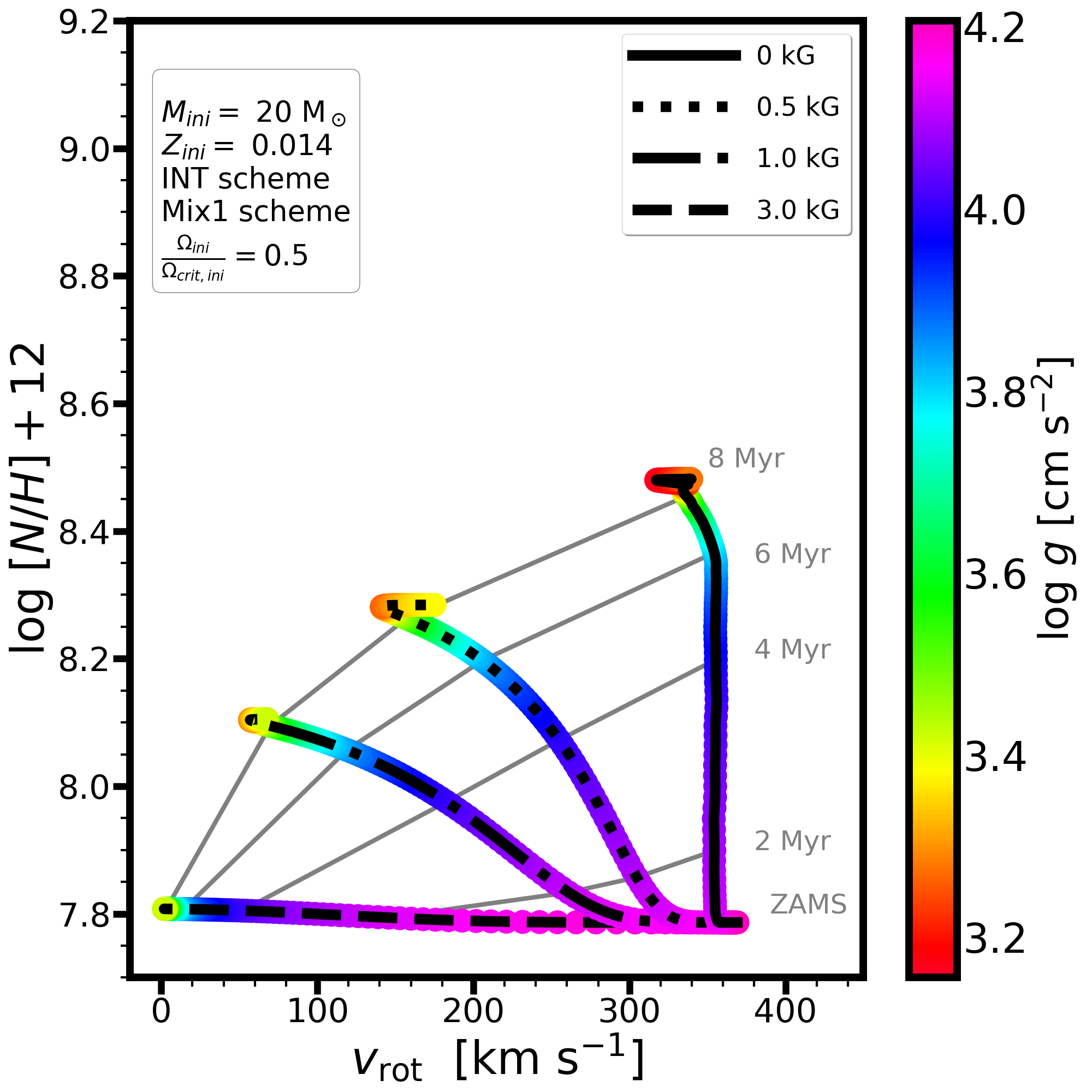
Figure 18: Hunter diagrams of the fiducial 20 M_⊙ models. Left: varying the initial magnetic field strength for given metallicity, braking, and mixing schemes. Right: varying the initial metallicity representative of solar, LMC, and SMC environments for 1 kG initial field strength.

In Figure 18, we follow the evolution of our 20 M_⊙ fiducial models on the Hunter diagram (Hunter et al., 2008, 2009), showing surface nitrogen abundance against the rotational velocity. The ZAMS is at the lower right corner of the diagrams with high surface gravities (colour-coded).

First, we demonstrate how a competition between magnetic braking and rotational mixing alters the evolutionary tracks (see also Paper III). The left panel of Figure 18 shows how the magnetic field strength results in drastic changes of the model predictions. The stronger the magnetic field, the more rapidly rotation brakes, and the less nitrogen can be mixed to the stellar surface. Above a given magnetic field strength, which strongly depends on other stellar and mixing parameters, the braking is efficient enough that nitrogen is not mixed to the surface and the observable nitrogen abundance remains the initial value throughout the main sequence. For the case of the 20 M_⊙ solar-metallicity model with the INT/Mix1 scheme shown in Figure 18, this threshold occurs roughly at 3 kG.

The right panel of Figure 18 reveals the impact of the initial metallicity on the evolution of the 20 M_⊙ INT/Mix1 models in the Hunter diagram. The initial equatorial magnetic field strength is chosen to be 1 kG. Consistently with previous findings (see Section 3.2.6), we obtain that chemical mixing is easier to trace in lower metallicity environments where the fractional change between the initial and final abundances are much larger (factor of $\sim~{}8$ at SMC metallicity) than at higher metallicity (factor of $\sim~{}2$ at solar metallicity) for the same fiducial model.

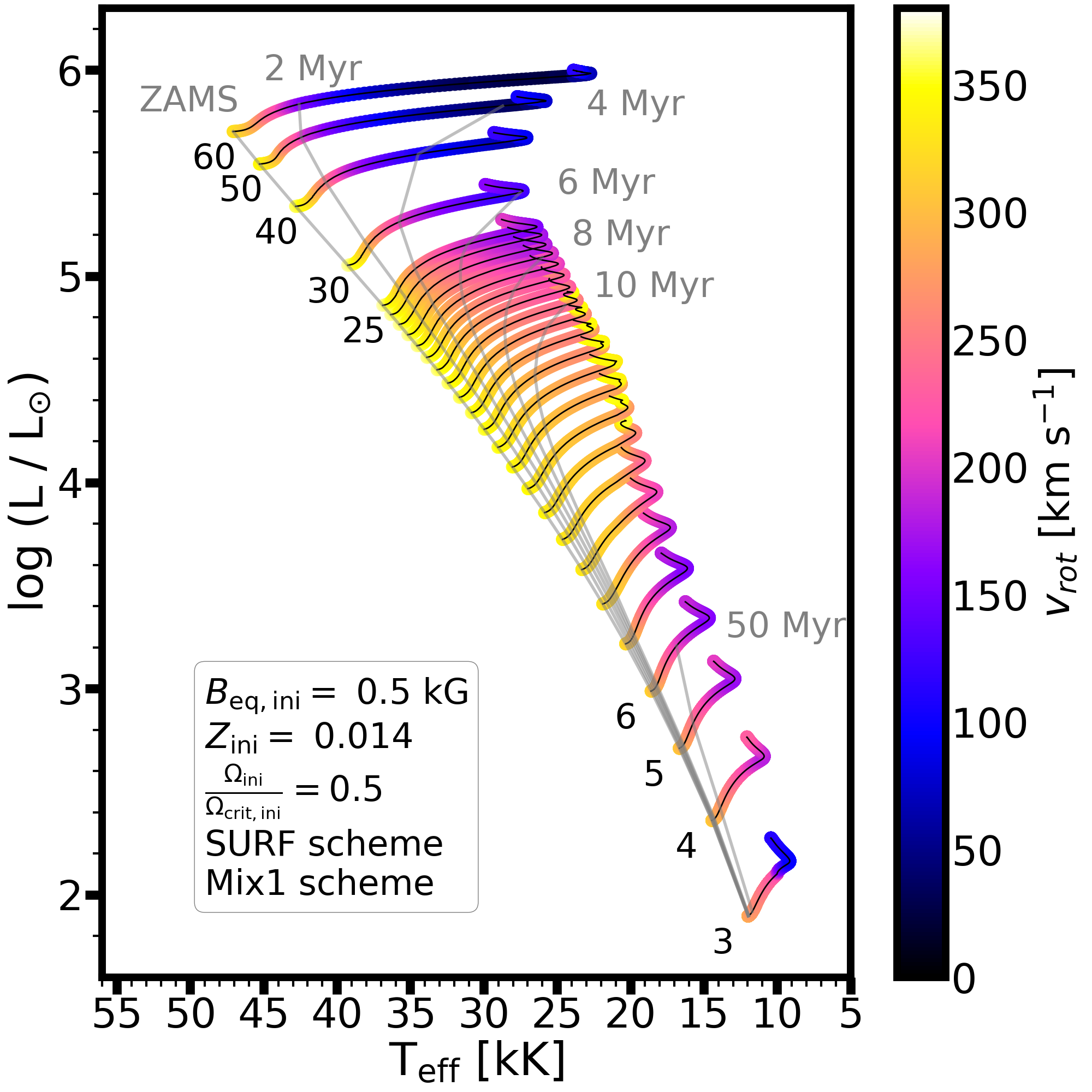
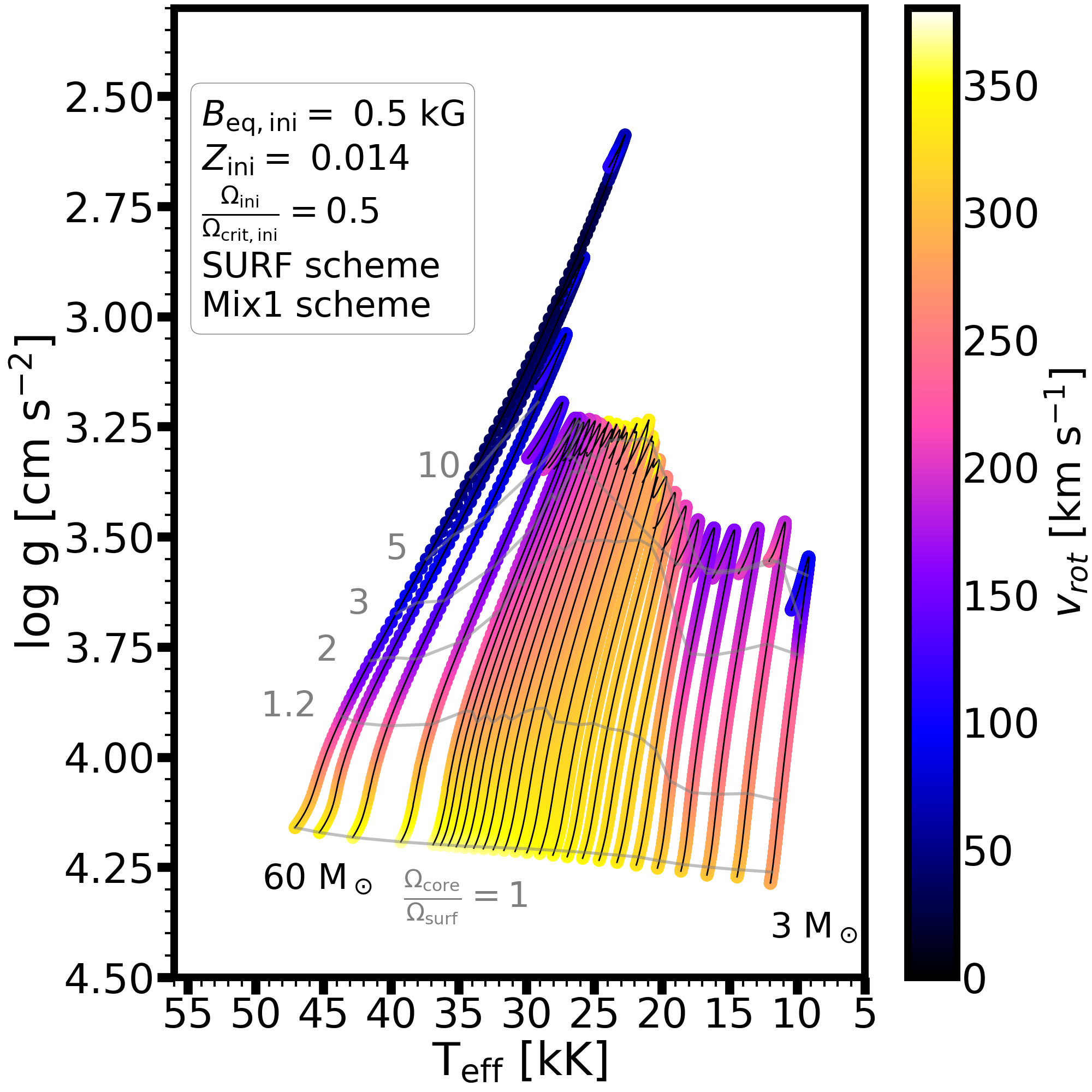
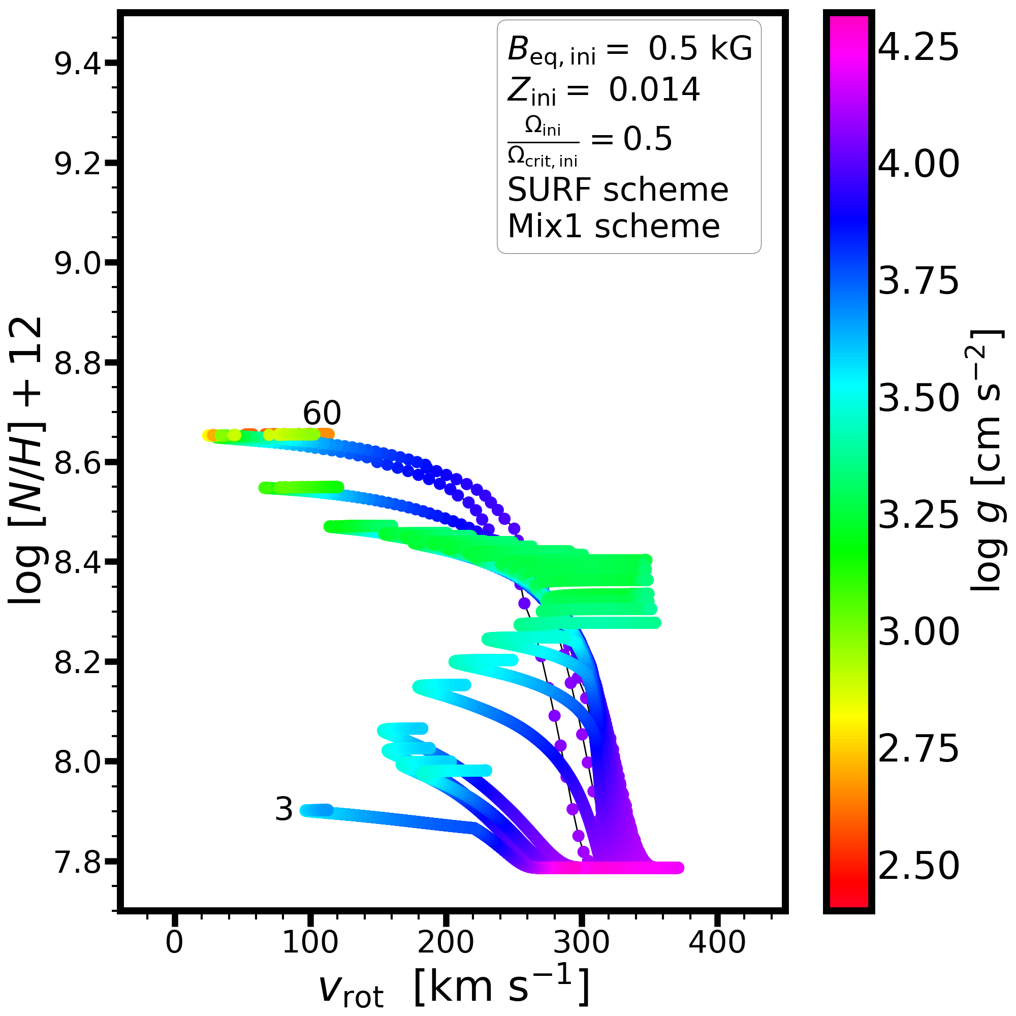
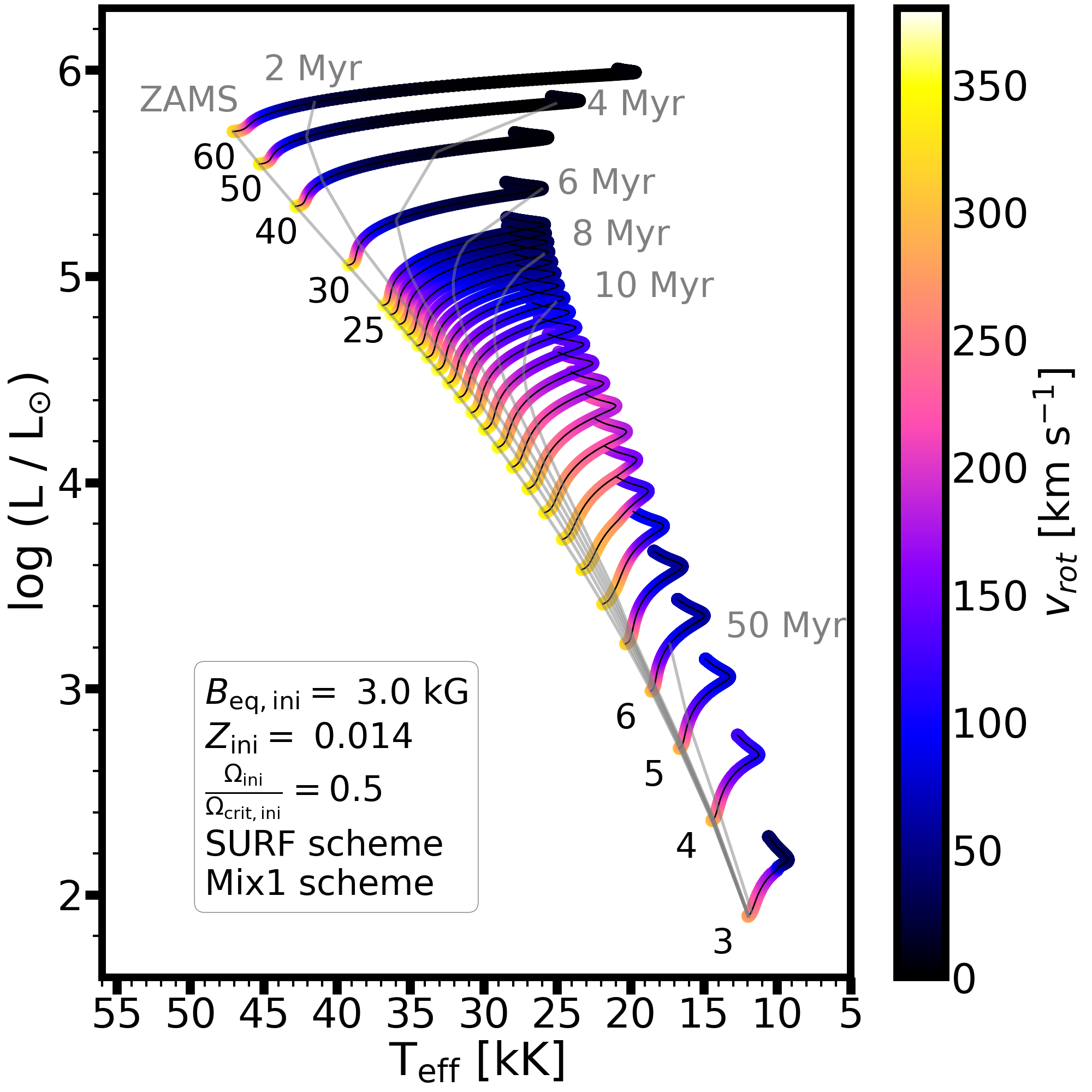
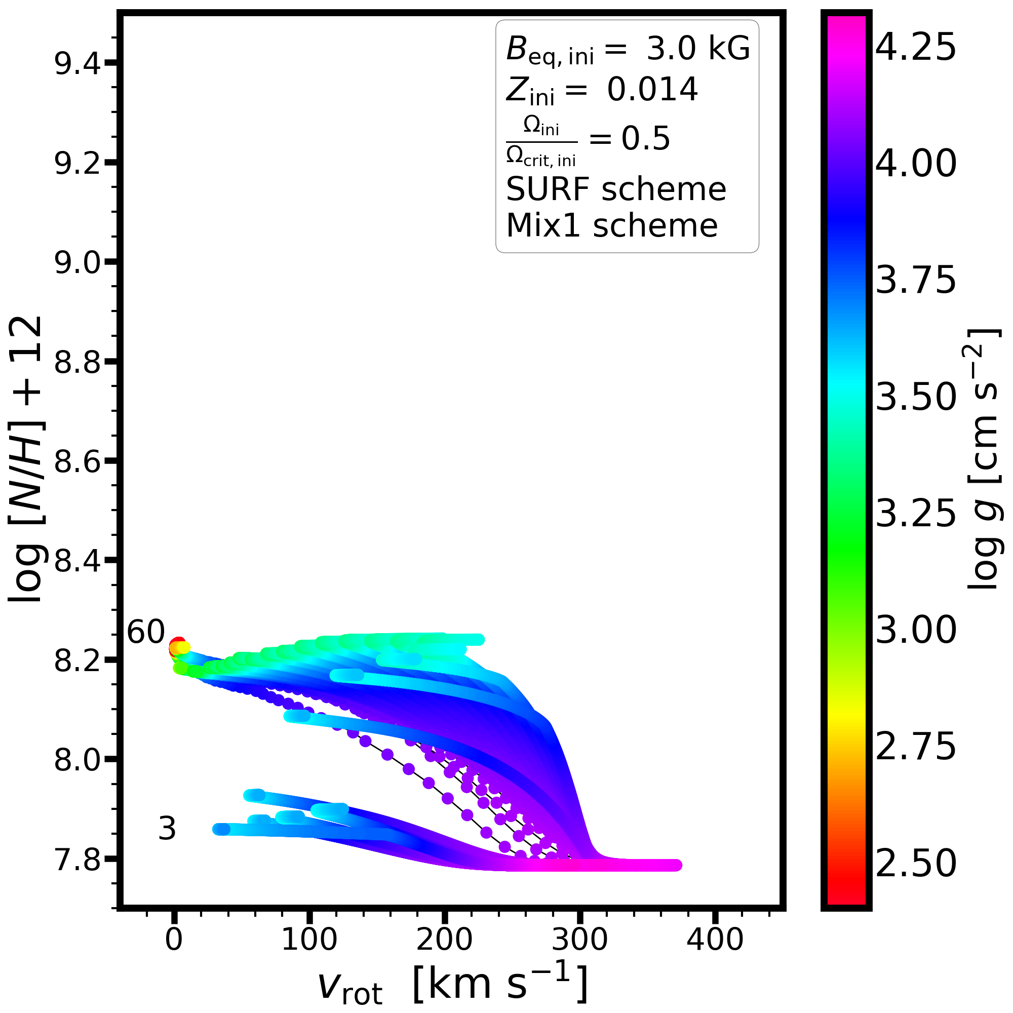
Figure 19: Same as Figure 9 but for the SURF/Mix1 scheme. Top panels show models with an initial equatorial magnetic field strength of 0.5 kG, whereas the lower panels show models with 3 kG. The NOMAG/Mix1 model is presented in Figure 9.

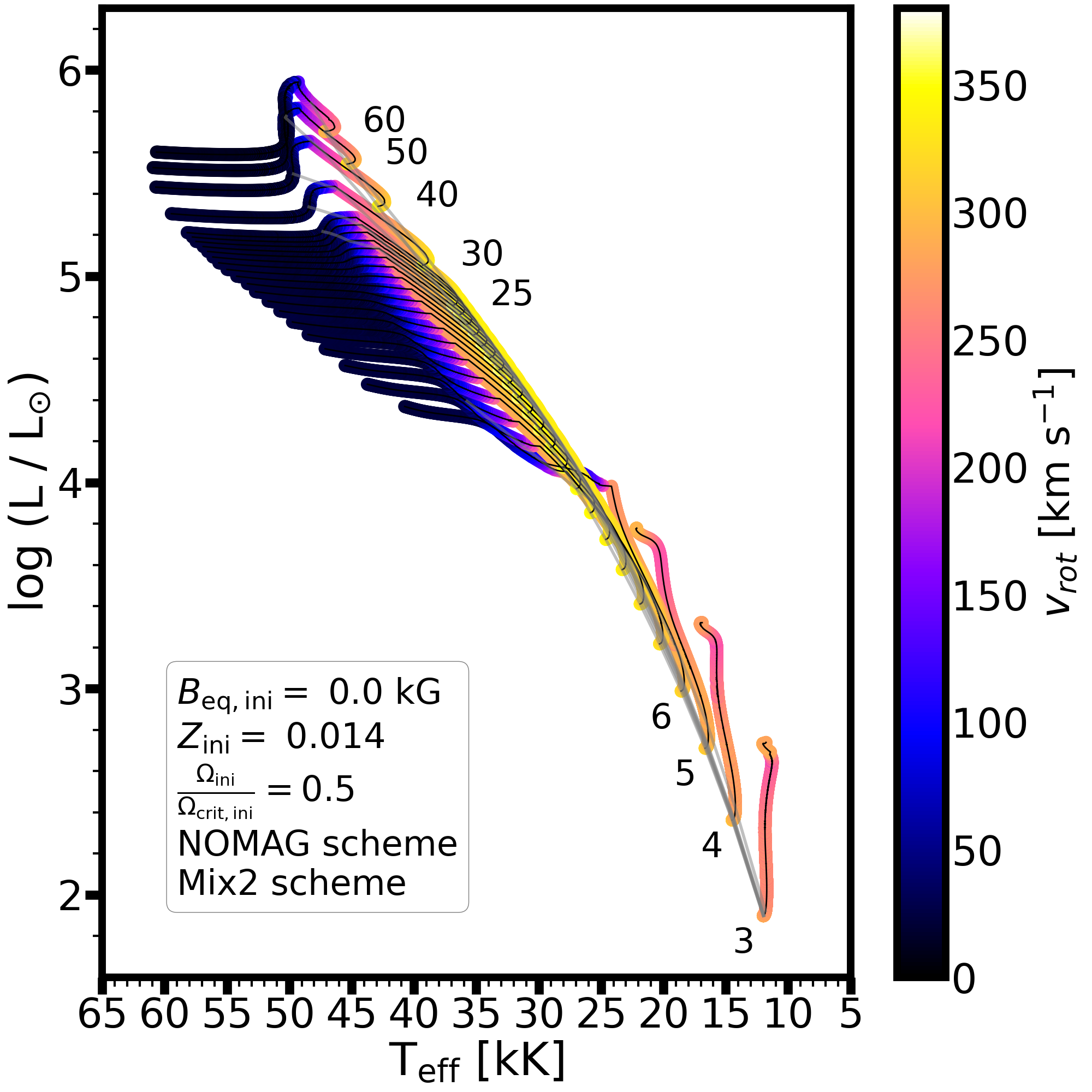
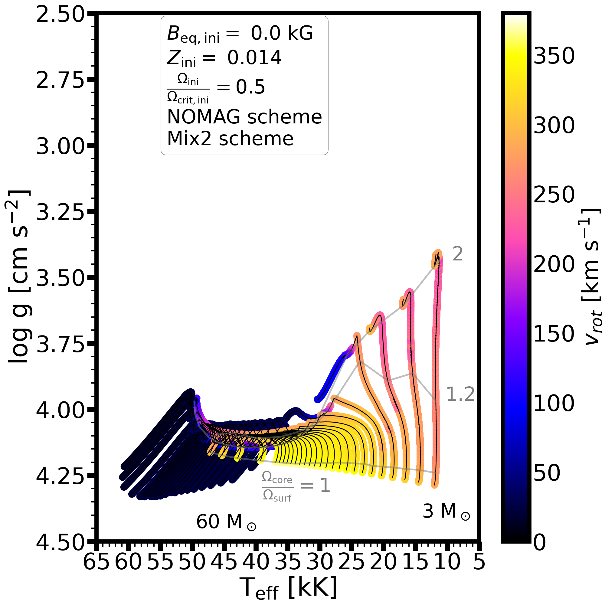
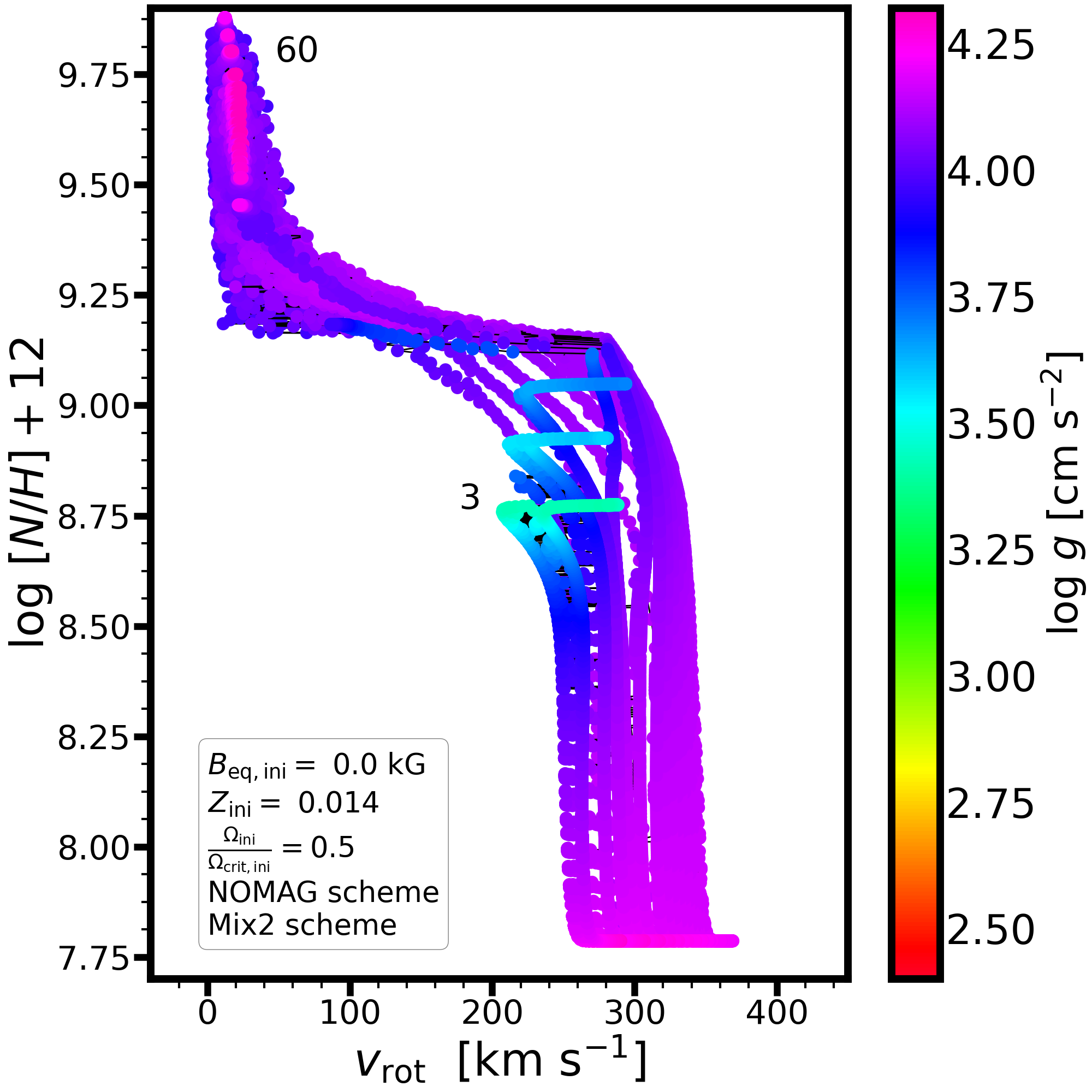
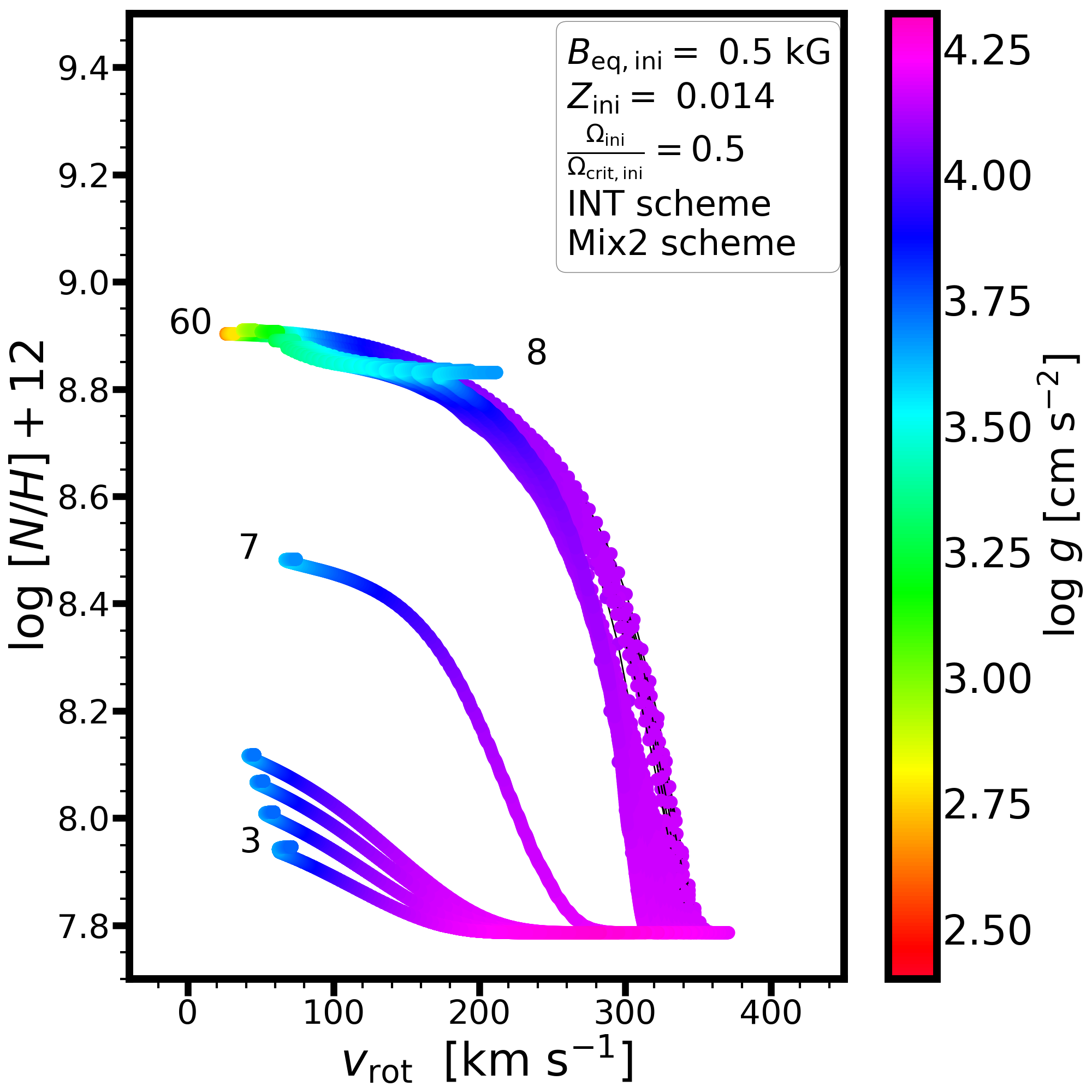
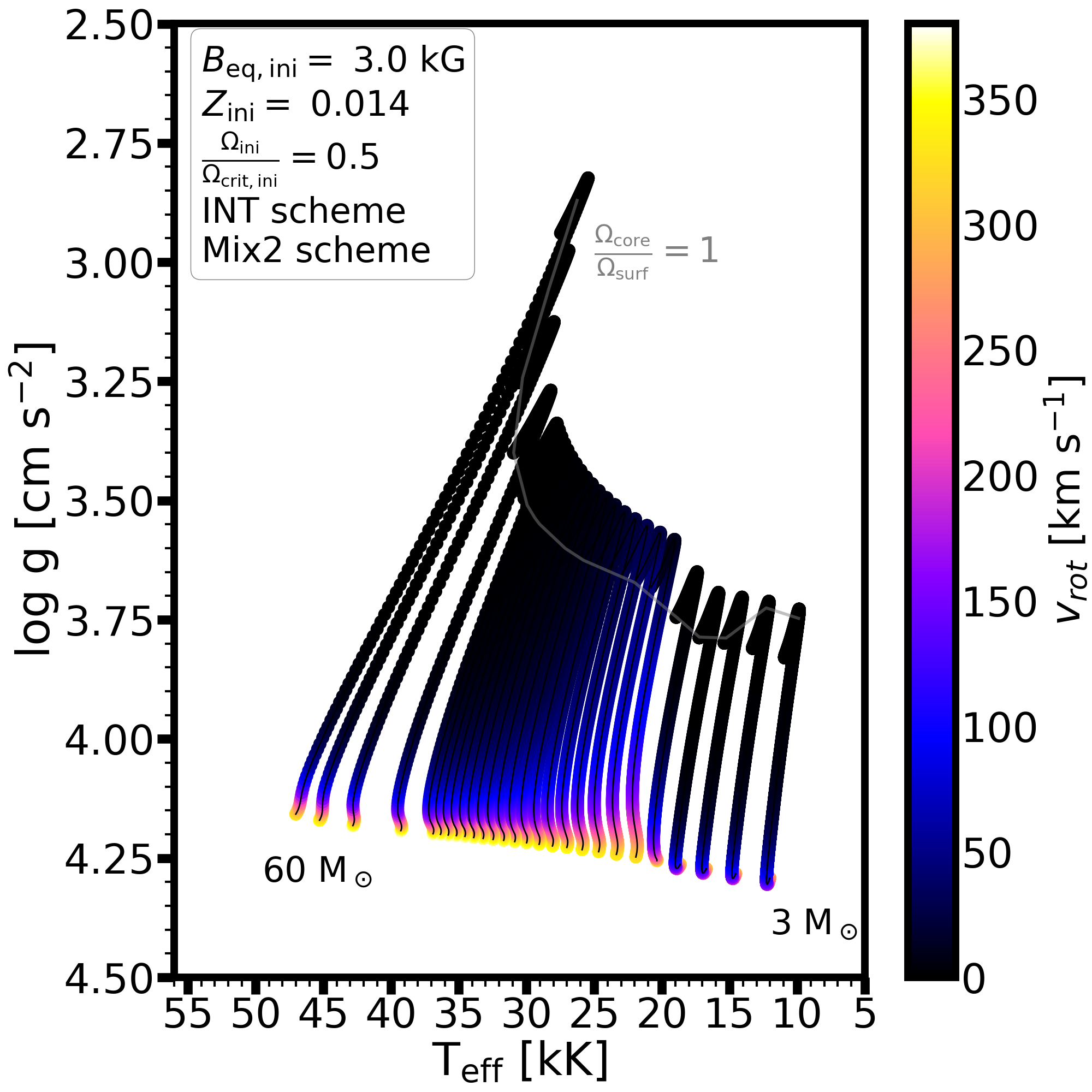
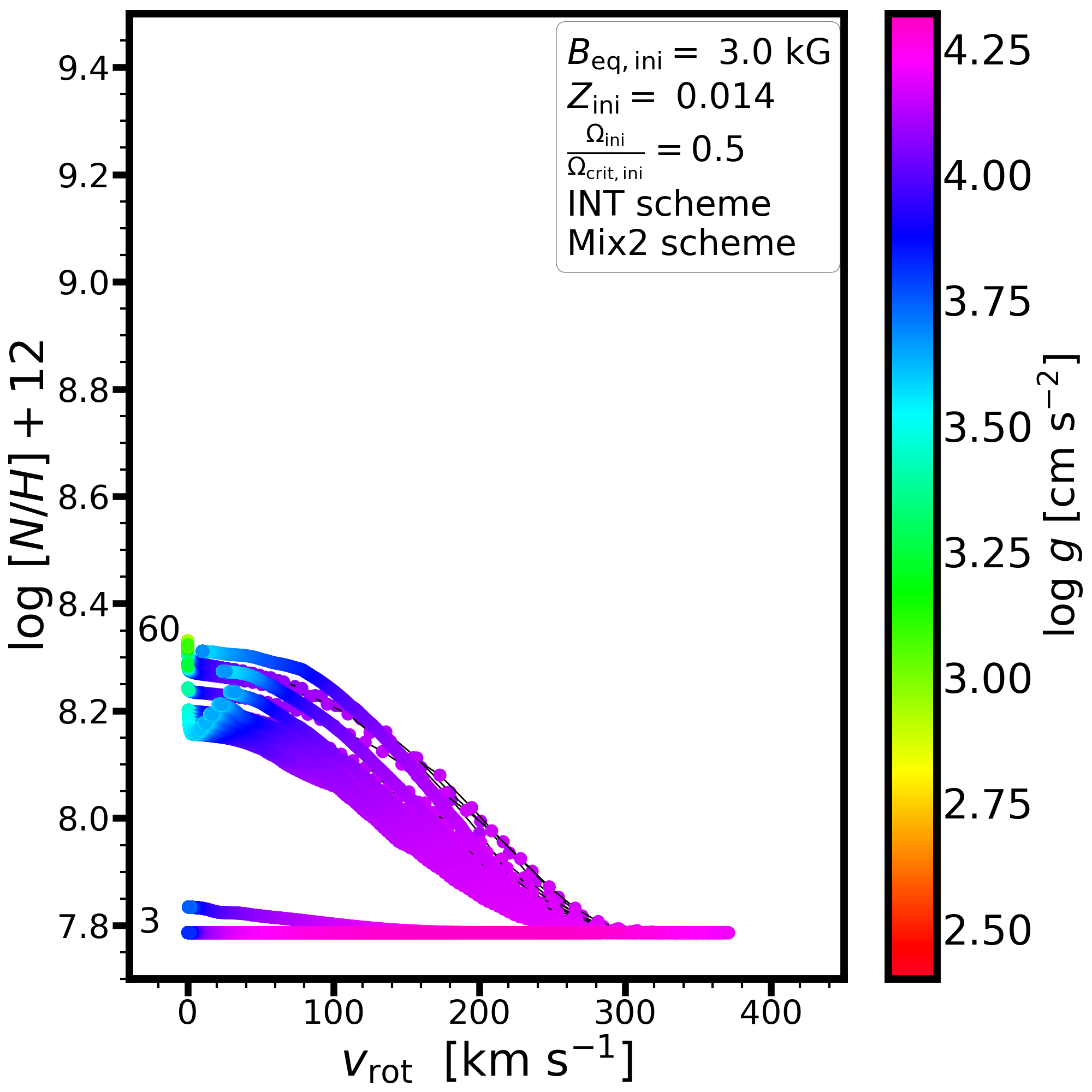
Figure 20: Same as Figure 9 but for the NOMAG/Mix2 (top panels) and INT/Mix2 (middle and lower panels) schemes.

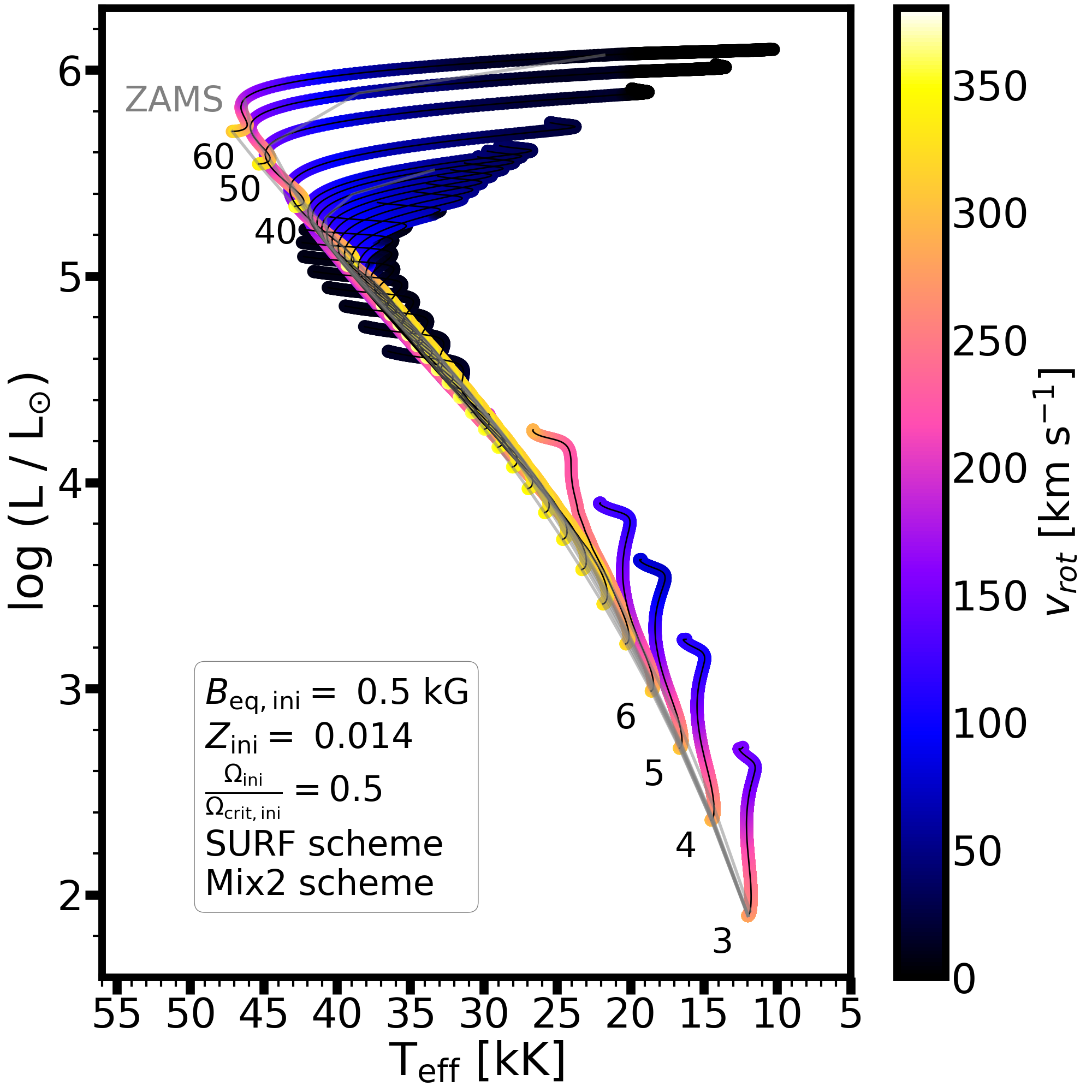
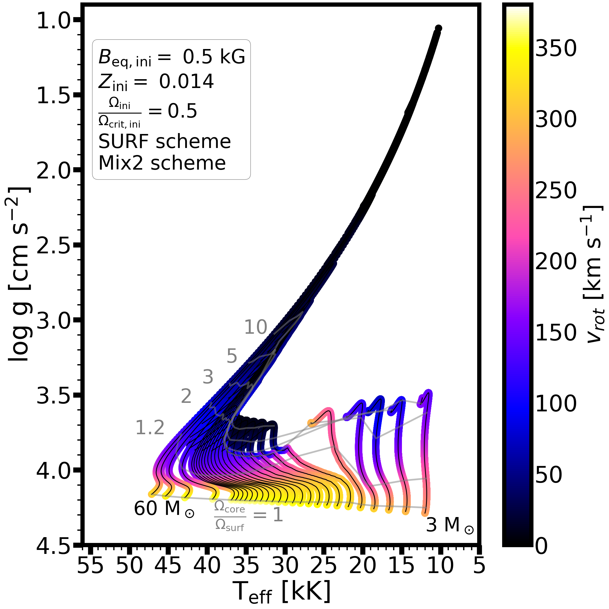
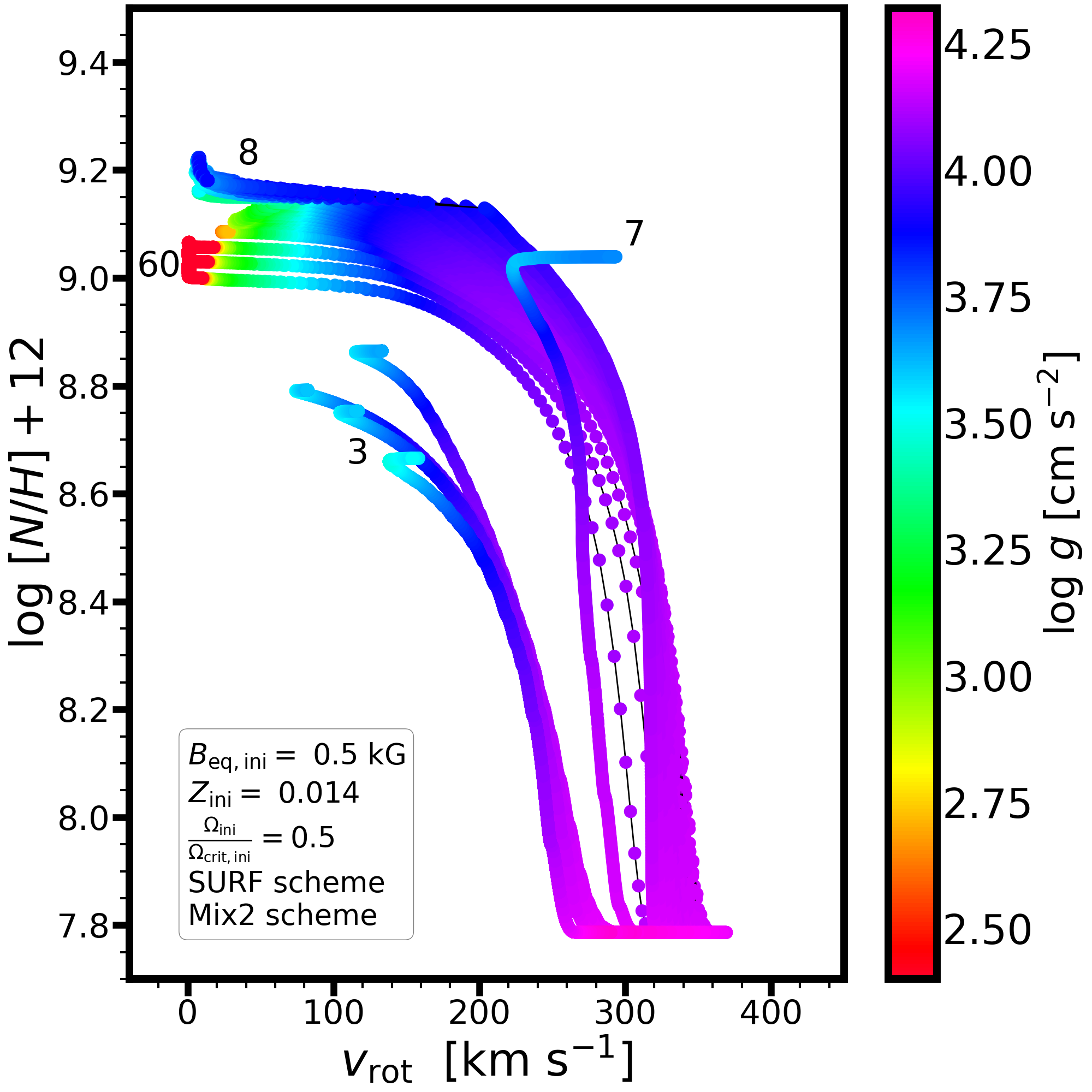
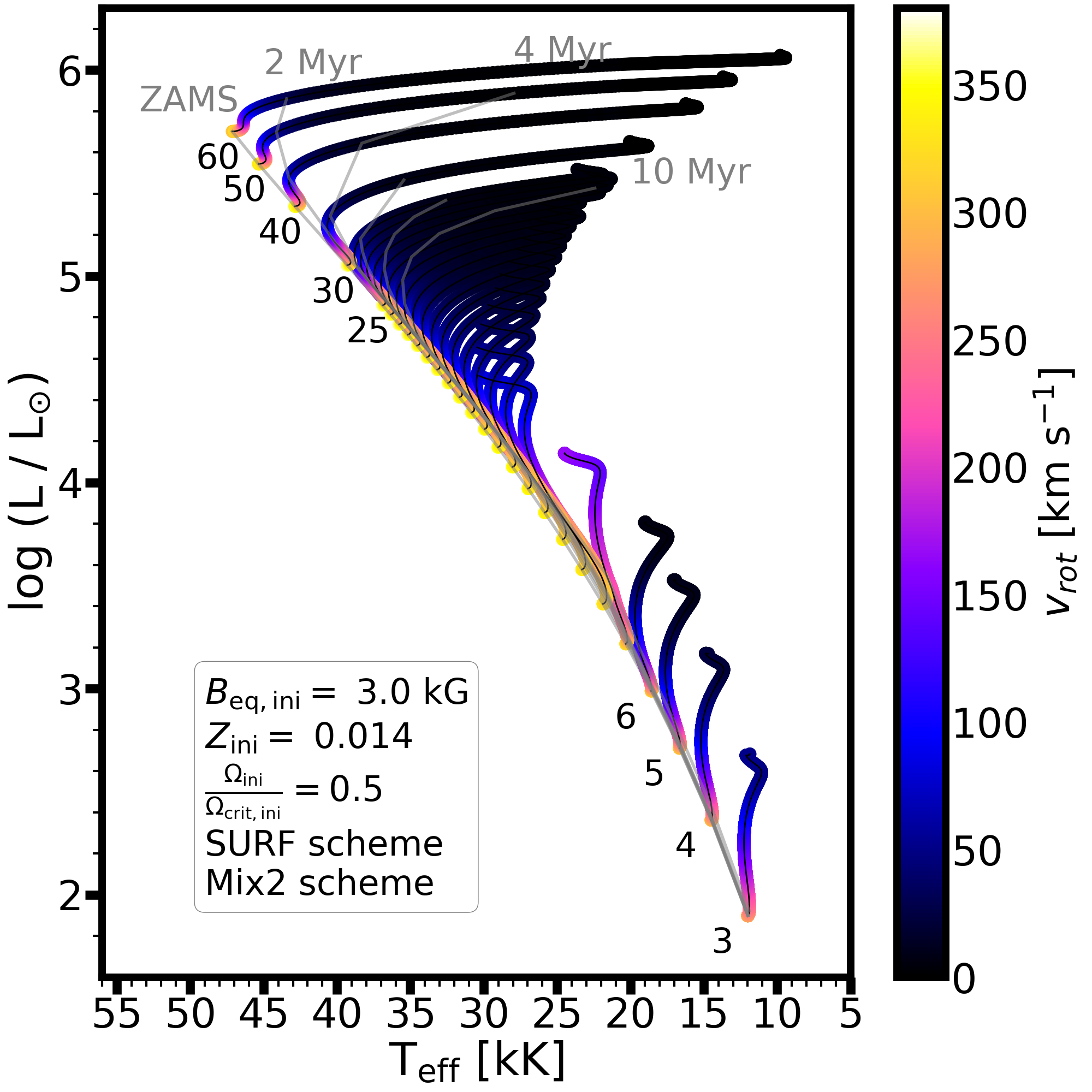
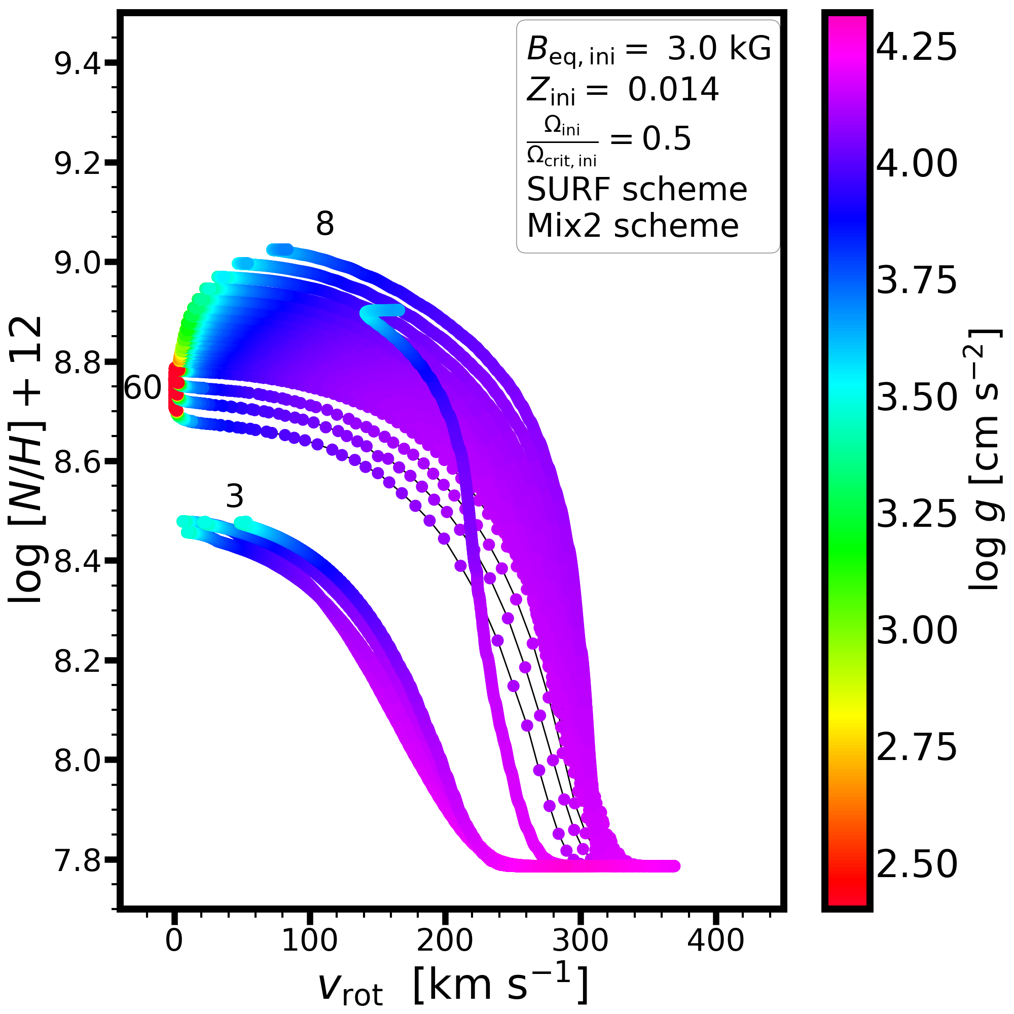
Figure 21: Same as Figure 9 but for the SURF/Mix2 scheme. See top panels of Figure 20 for the NOMAG/Mix2 models.

E.2 Impact of varying magnetic field strength within the other braking and mixing schemes at solar metallicity

Here, we describe the effect of varying the magnetic field strength for the stellar evolution when accounting for the INT magnetic braking scheme in combination with the Mix2 chemical mixing scheme and the SURF magnetic braking scheme in combination with both the Mix1 and Mix2 chemical mixing schemes at solar metallicity. We display the evolutionary tracks for these models with initial magnetic field strengths of 0.5 and 3 kG in Figures 19, 20, and 21. The NOMAG/Mix1 models are shown in Figure 9 and the NOMAG/Mix2 models are shown in Figure 19. This is complementary to the description in Section 3.2.5 and Figure 9 for varying the magnetic field strength when using the INT magnetic braking scheme and the Mix1 chemical mixing scheme. Below, we first describe how the stellar evolution is affected by accounting for magnetic fields for each of the SURF/Mix1, INT/Mix2, and SURF/Mix2 cases.

E.2.1 SURF/Mix1

As described in Section 3.2 and seen from Figure 9, when the Mix1 rotational mixing scheme is used without including magnetic fields, the stars with initial masses $<30$ M_⊙ remain rapidly rotating ($>200$ km s^-1) until the end of the main sequence. The nitrogen abundance increases smoothly (compared to the initial value, see Table 2) with the initial mass, stretching from $\log(N/H)+12=8.0$ up to $8.8$. The stars develop mild differential rotation as the main sequence progresses, resulting in cores spinning roughly twice as fast as their envelopes towards the end of the main sequence.

When treating magnetic fields using the SURF scheme, angular momentum is very efficiently transported in the outermost 20% of the mass. In deeper layers of these models efficient shear mixing is invoked by differential rotation (see Section 3.1). As a result, mixing is enhanced in magnetic models treated with the SURF scheme compared to those treated with the INT scheme, which in contrast are rigidly rotating. Nitrogen is mixed out more efficiently, reaching surface abundances up to $\log(N/H)+12=8.7$ in the SURF models compared to 8.6 in the INT models of stars with initial equatorial magnetic field strength of 0.5 kG. This can be seen when comparing the middle row of Figure 9 with the top row of 19. In fact, for stars with initial equatorial magnetic field strength of 0.5 kG in the SURF/Mix1 scheme, the surface enrichment of nitrogen is very similar throughout the main-sequence as for the corresponding non-magnetic models. However, the stars spin down somewhat more when magnetic fields are implemented.

In the bottom row of Figure 19, models with initial equatorial magnetic field strength of 3 kG are displayed. From these models it is even more evident that the SURF scheme gives rise to slower spin-down than the INT scheme does (cf. the bottom row of Figure 9). While some stars still have a considerable rotational velocity at the end of the main-sequence, magnetic braking is sufficient to produce less enriched stars with nitrogen abundances of $\log(N/H)+12=8.3$. When the INT scheme is implemented instead, none of the models with initial magnetic field strength of 3 kG exhibit nitrogen-enriched surfaces.

E.2.2 INT/Mix2

The Mix2 chemical mixing scheme is an efficient rotational mixing scheme, resulting in quasi-chemically homogeneous main-sequence evolution when magnetic fields are not taken into account (see Section 3.1 and Figure 5). The evolution of the non-magnetic models is displayed in the upper row of panels of Figures 20. We can see that non-magnetic stars are expected to experience modest differential rotation (since a high diffusivity, which we attributed to the magnetic field, is not assumed in these models). All of the non-magnetic models efficiently mix nitrogen out to the surface, reaching values of $\log(N/H)+12$ of 8.8-9.5. All but the most massive stellar models remain rapidly rotating throughout most of the main sequence, with surface rotation speeds of $\sim 200-350$ km s^-1.

In the middle row of Figure 20, we display models initialised with 0.5 kG magnetic field strengths according to the INT scheme. This magnetic field strength is sufficient to brake the rotation of the stars, but only after a significant amount of nitrogen has been mixed out to the surface. As a result, all stars rotate slower than $\sim 50$ km s^-1 once the TAMS is reached, and stars with initial masses above 7 $M_{\odot}$ have surface nitrogen abundances of $\log(N/H)+12\sim 8.9$. As visible from the colour-coding in the Kiel diagram, both the most massive and least massive stars spin down early during the main-sequence evolution, while the models in the intermediate-mass range of $\sim 5-10$ M_⊙ spin down later during the main-sequence evolution (see Section 3.2.4).

As seen from Figure 20, a modest initial magnetic field strength of 0.5 kG is sufficient to completely alter the evolution in the Hertzsprung-Russell diagram. If magnetic fields are not accounted for, the stars are expected to evolve quasi-chemically homogeneously during the entire main sequence, which is not the case when magnetic fields are taken into account. In the Kiel diagrams, the ratios of the core to envelope spins are shown. When magnetic field effects are accounted for in the INT scheme, the models rotate rigidly throughout the main sequence (cf. Section 3.2.3).

In the case of models with initial magnetic field strength of 3 kG (bottom row of Figure 20), magnetic braking is even more efficient compared to the case of the 0.5 kG models. As a result, rotational mixing can only act briefly before the stars have spun down, leading to slow rotation rates of $\lesssim 50$ km s^-1 already in the beginning of the main sequence (for example when $\log g~{}\sim~{}4.0$). The maximum surface nitrogen abundances reached are also correspondingly low in comparison to the non-magnetic and weakly magnetic cases, reaching $\log(N/H)+12\sim 8.4$.

E.2.3 SURF/Mix2

Since stars spin down slower when the SURF scheme is used compared to the INT scheme to implement magnetic fields, the quasi-chemically homogeneous main sequence evolution that the non-magnetic models in the Mix2 rotational mixing scheme exhibit is not as easily quenched by the implementation of magnetic fields in the SURF/Mix2 combination. The effect of the weaker magnetic braking is evident when comparing Figures 20 and 21.

As a result of the slower spin-down, even stars with initial magnetic field strength of 3 kG still substantially enrich their surfaces with nitrogen ($\log(N/H)+12=8.7-9.2$). They also reach rotation rates close to zero at the end of the main sequence. As seen in Figure 5, the combination of SURF and Mix2 results in such efficient mixing that even the surface helium abundance significantly increases during the main sequence.

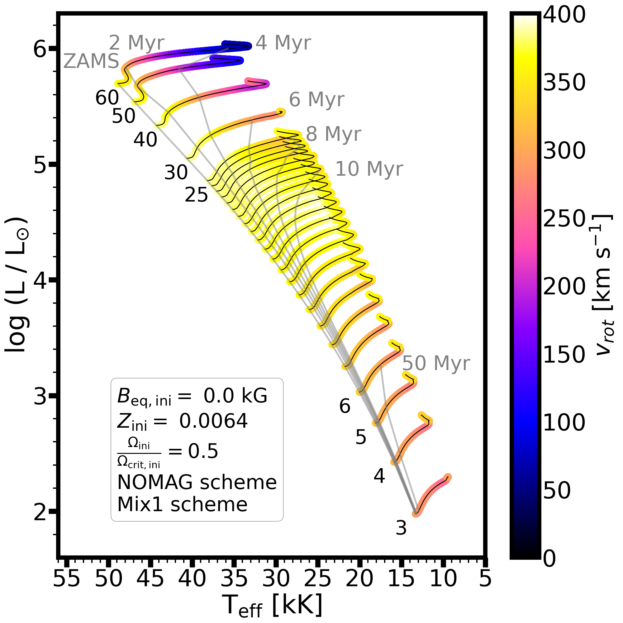
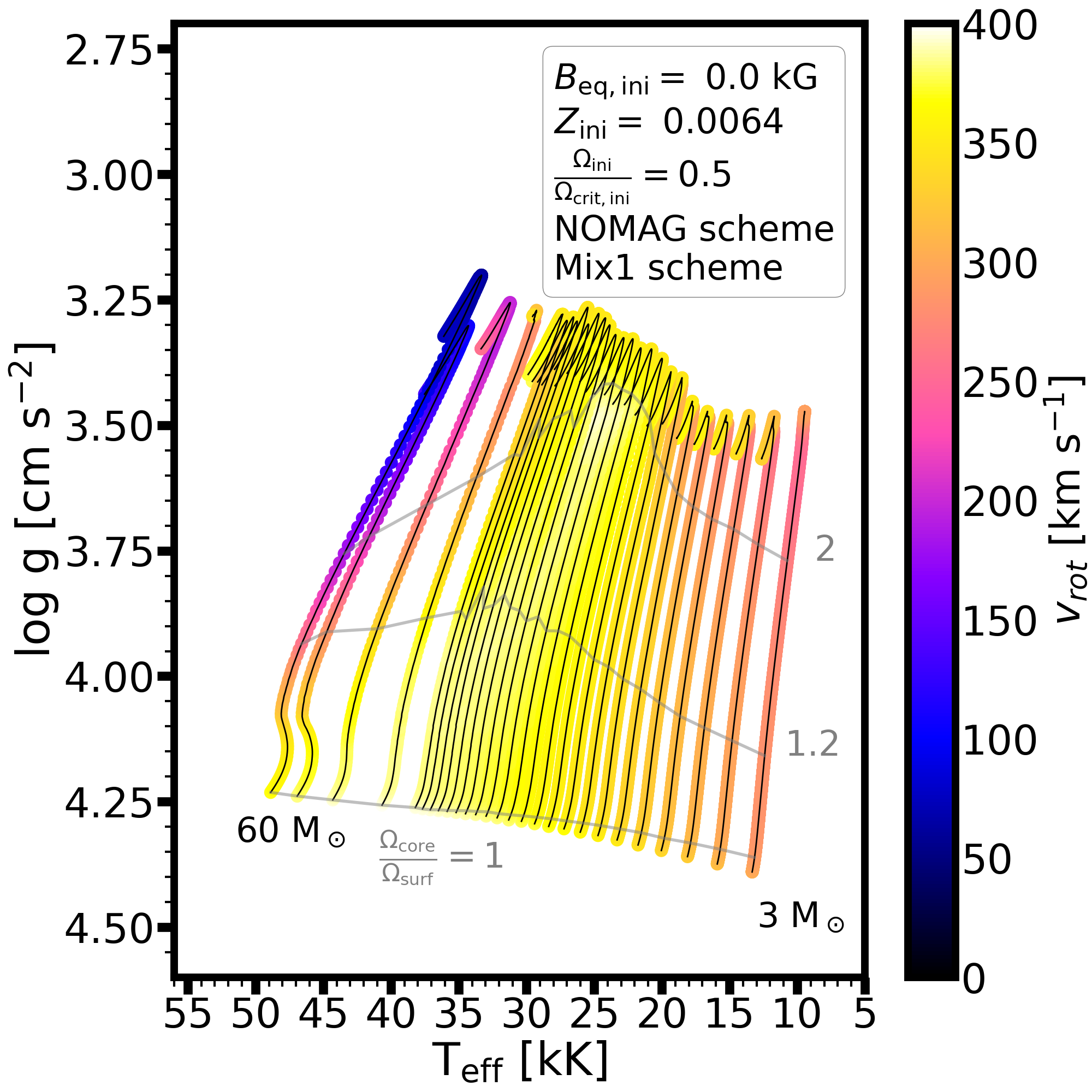
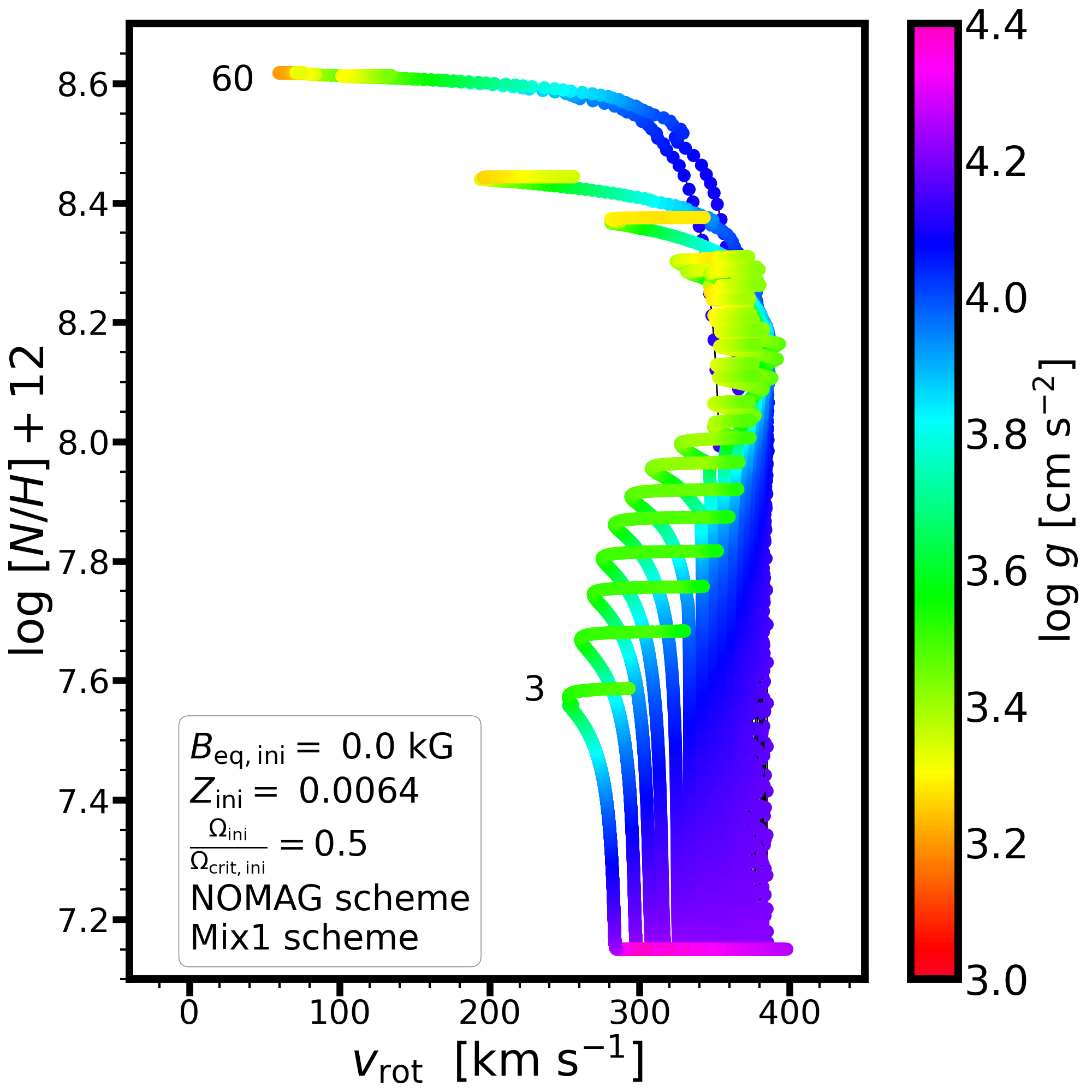
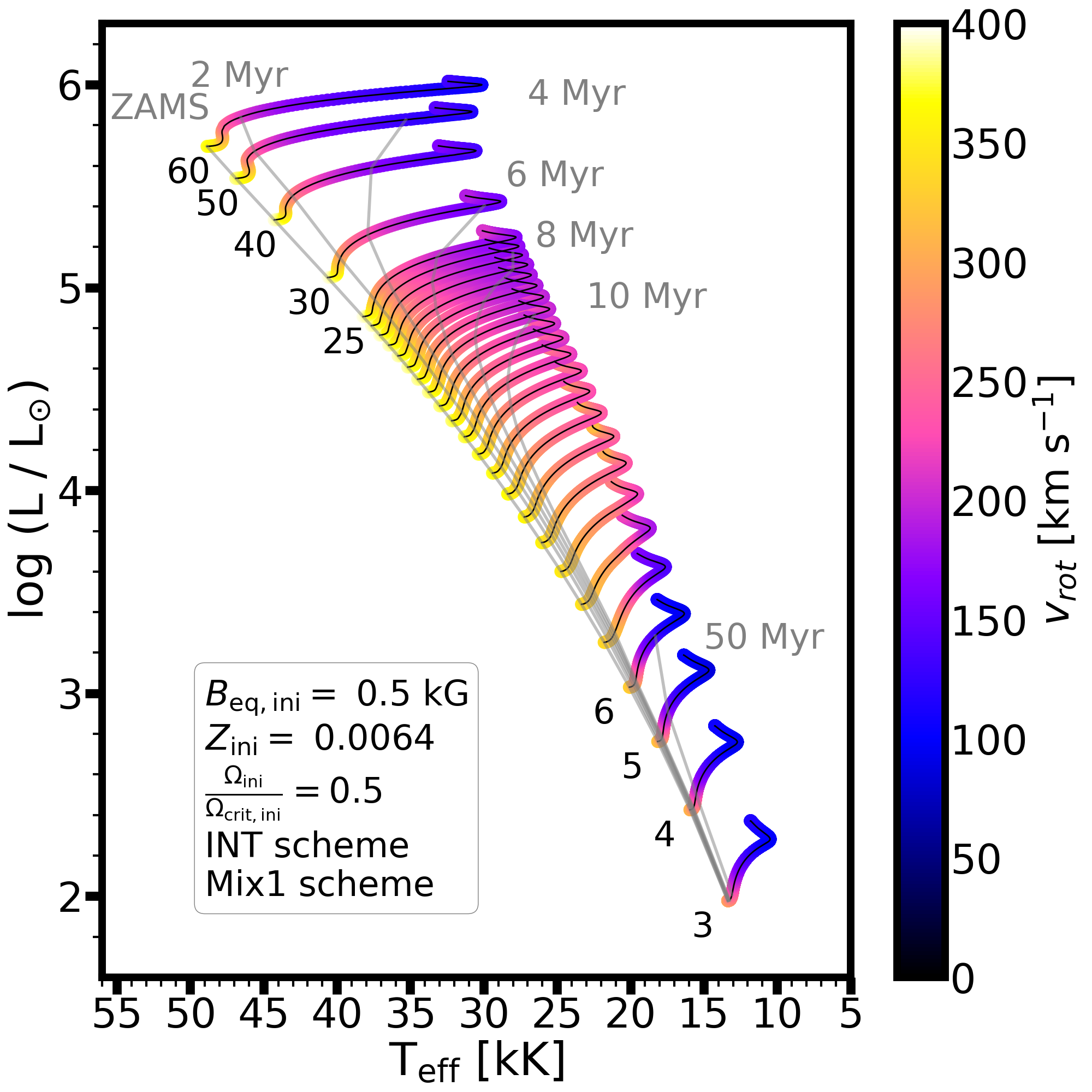
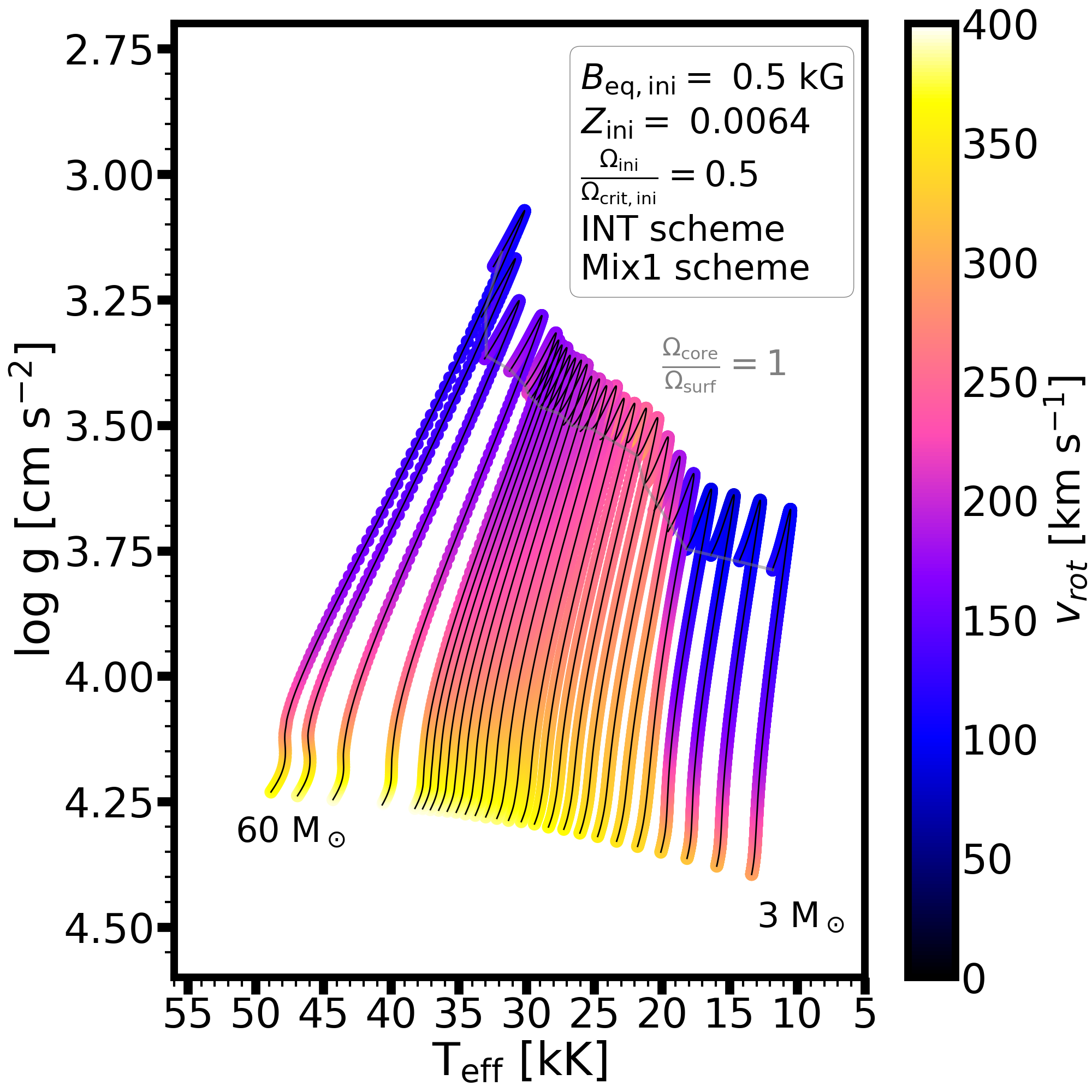
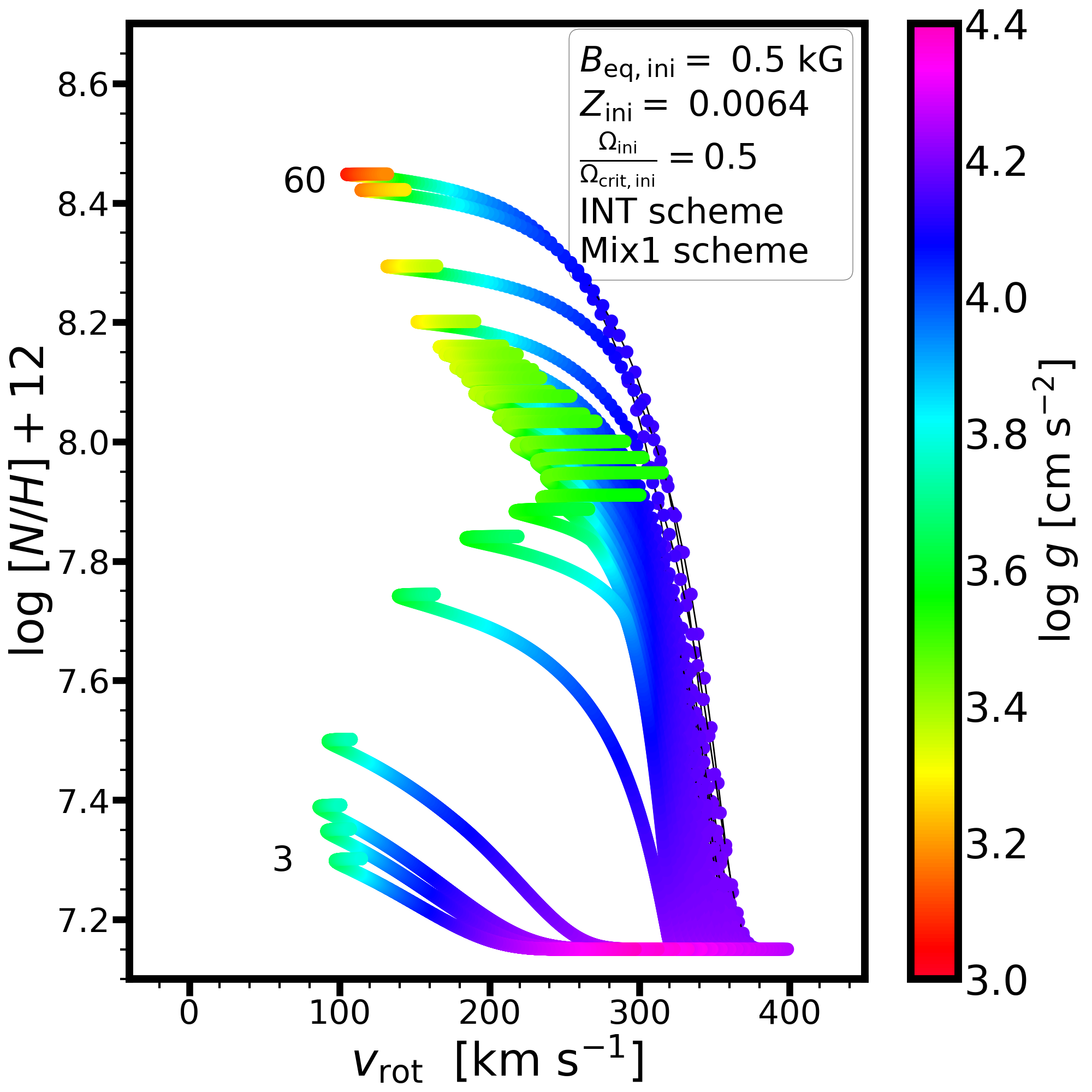
Figure 22: Same as Figure 9 but for the NOMAG/Mix1 scheme (top) and INT/Mix1 scheme with an initial equatorial magnetic field strength of 0.5 kG (lower panel) at $Z=0.0064$. The INT/Mix1 model with initial equatorial magnetic field strength of 3 kG is presented in Figure 10.

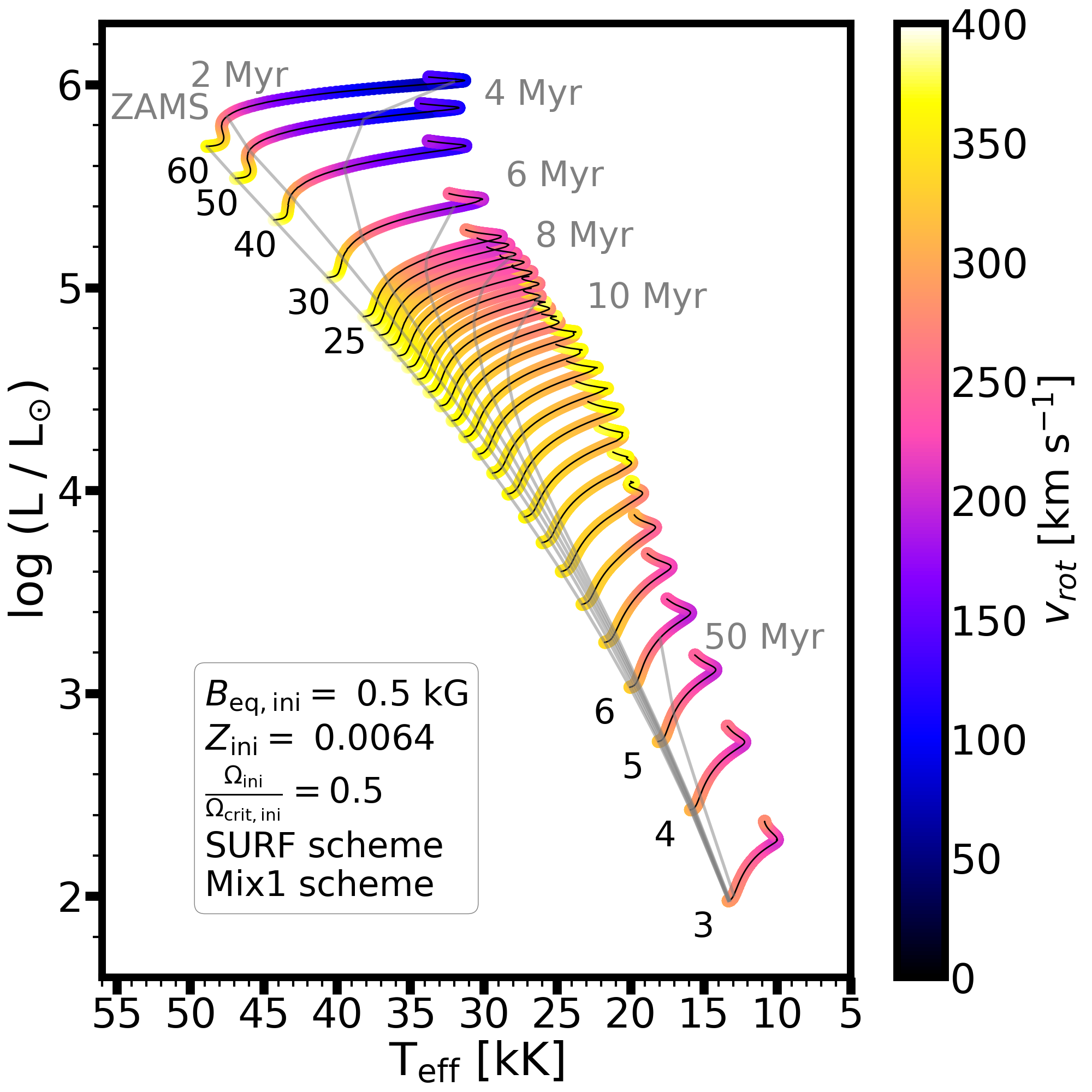
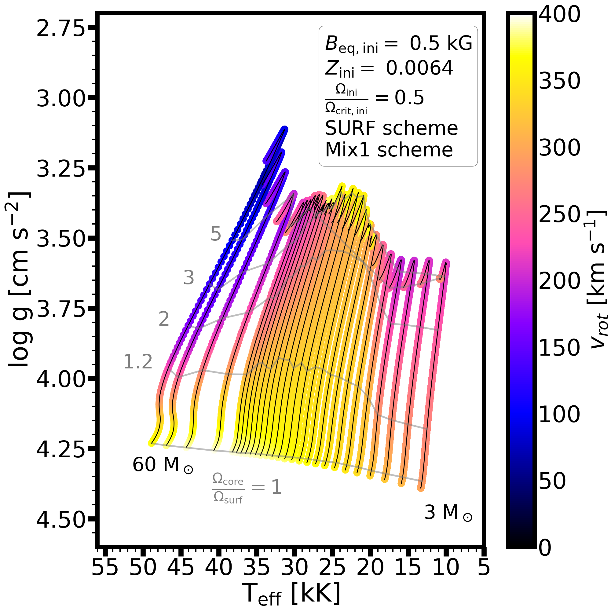
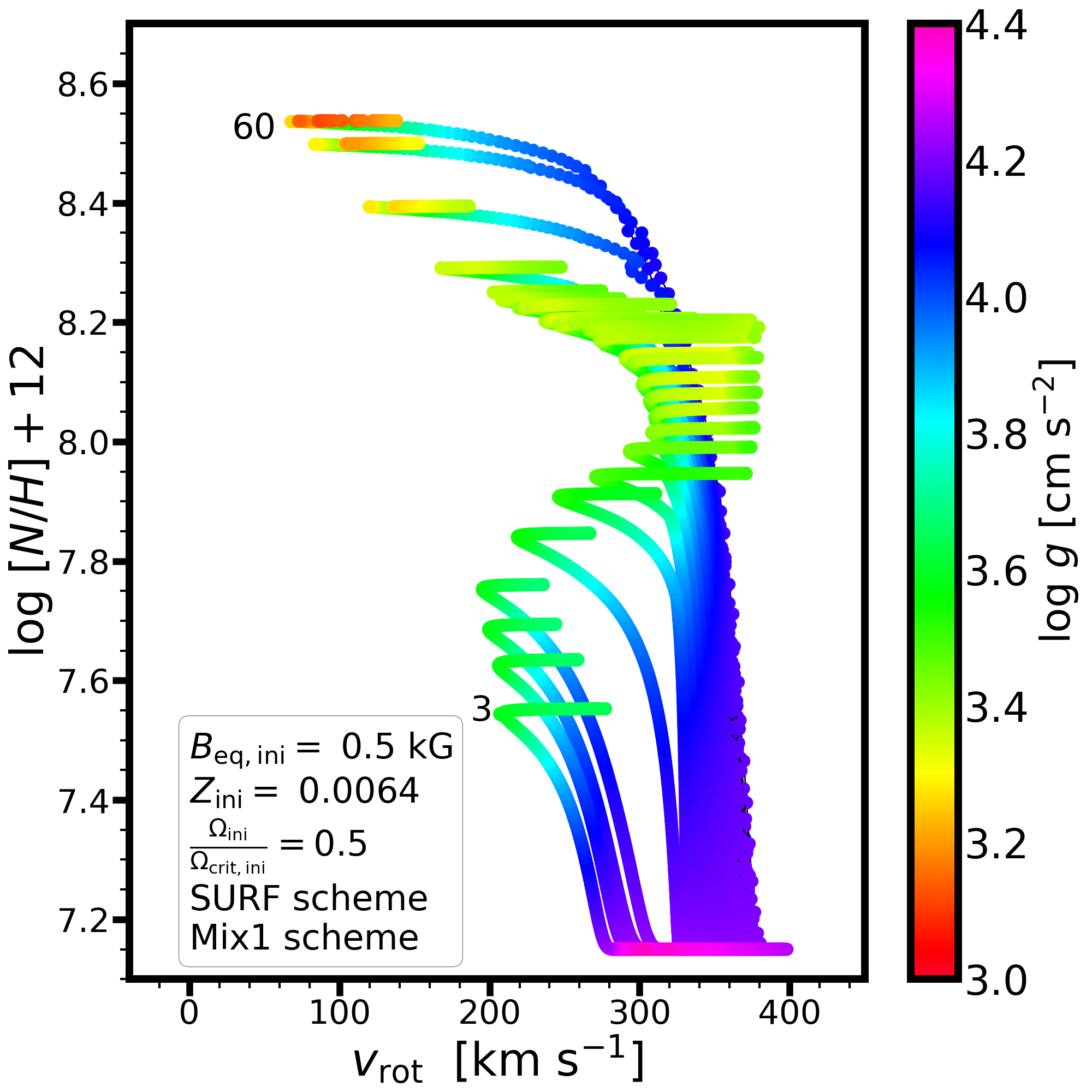
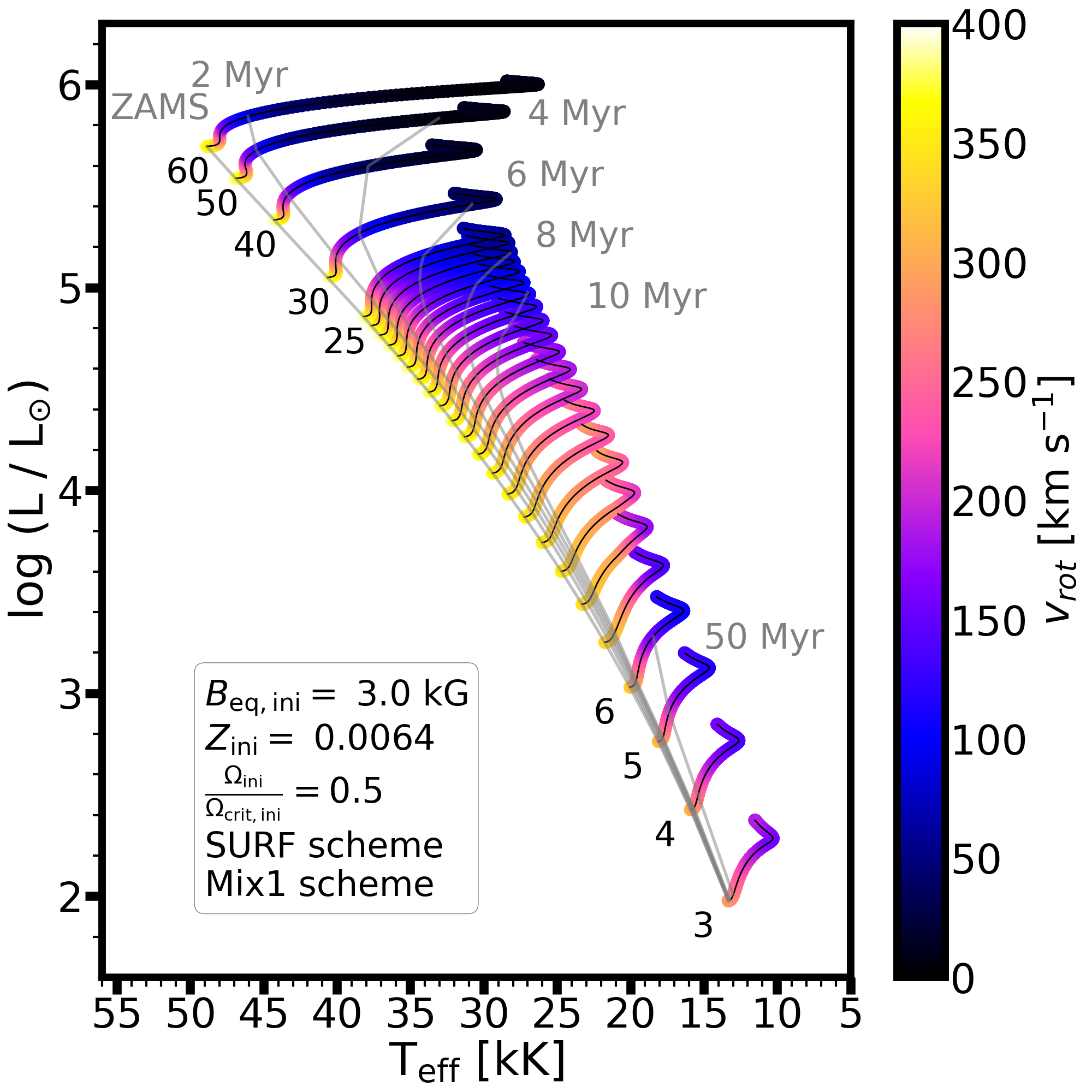
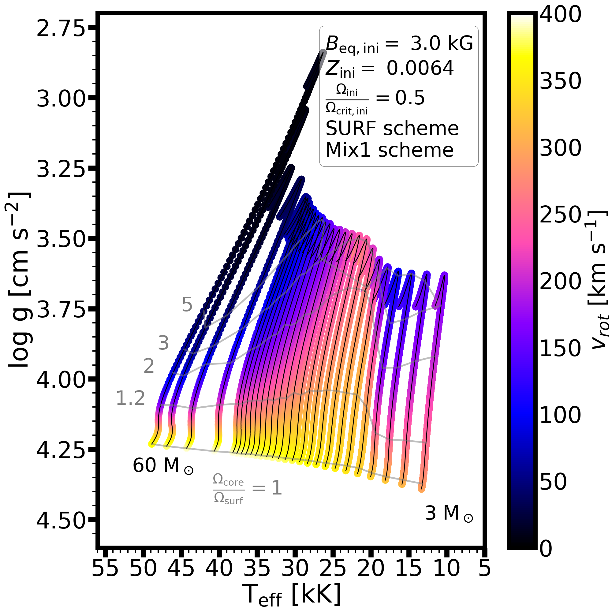
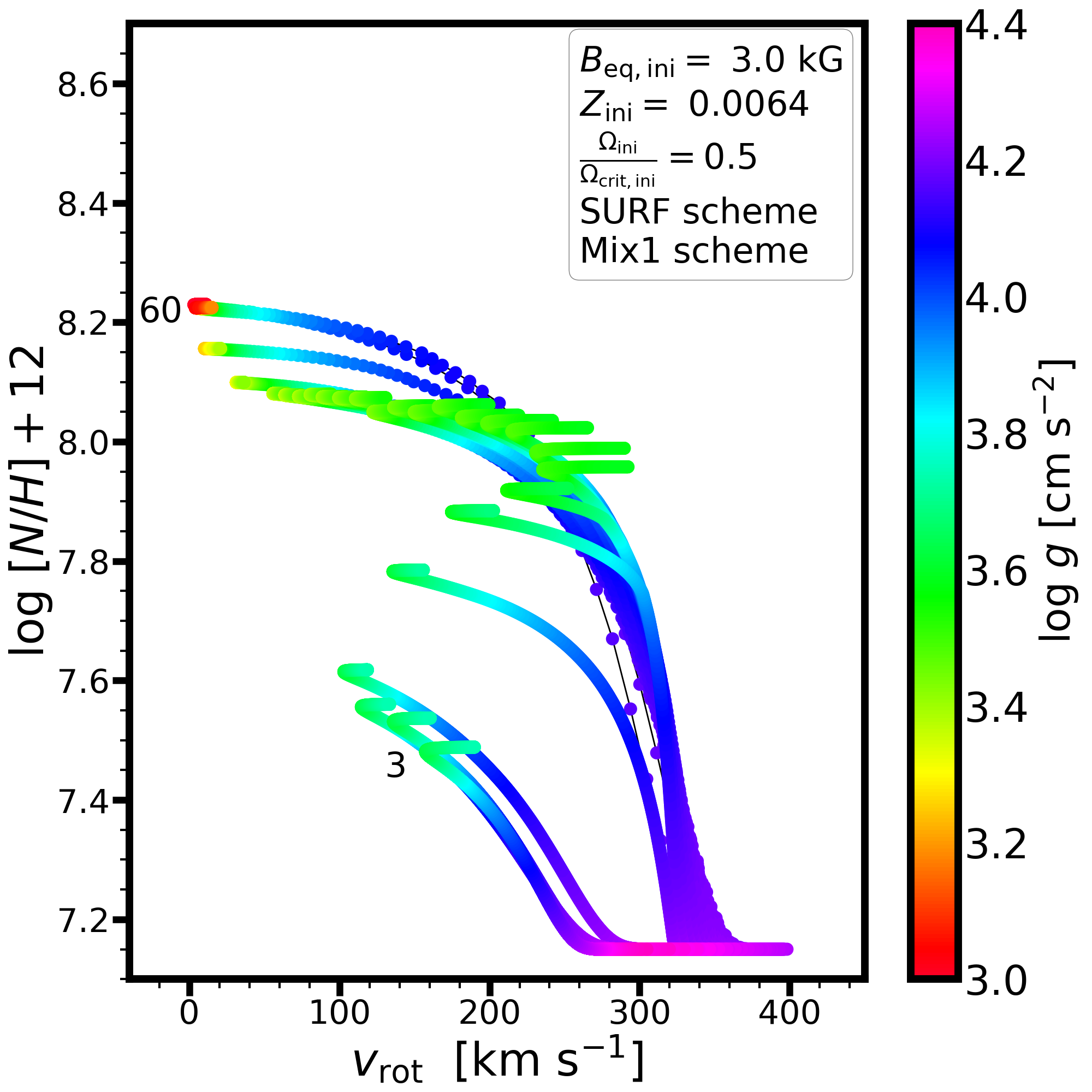
Figure 23: Same as Figure 22 but for the SURF/Mix1 scheme. Top panels show models with an initial equatorial magnetic field strength of 0.5 kG, whereas the lower panels show models with 3 kG. The NOMAG/Mix1 model is presented in Figure 22.

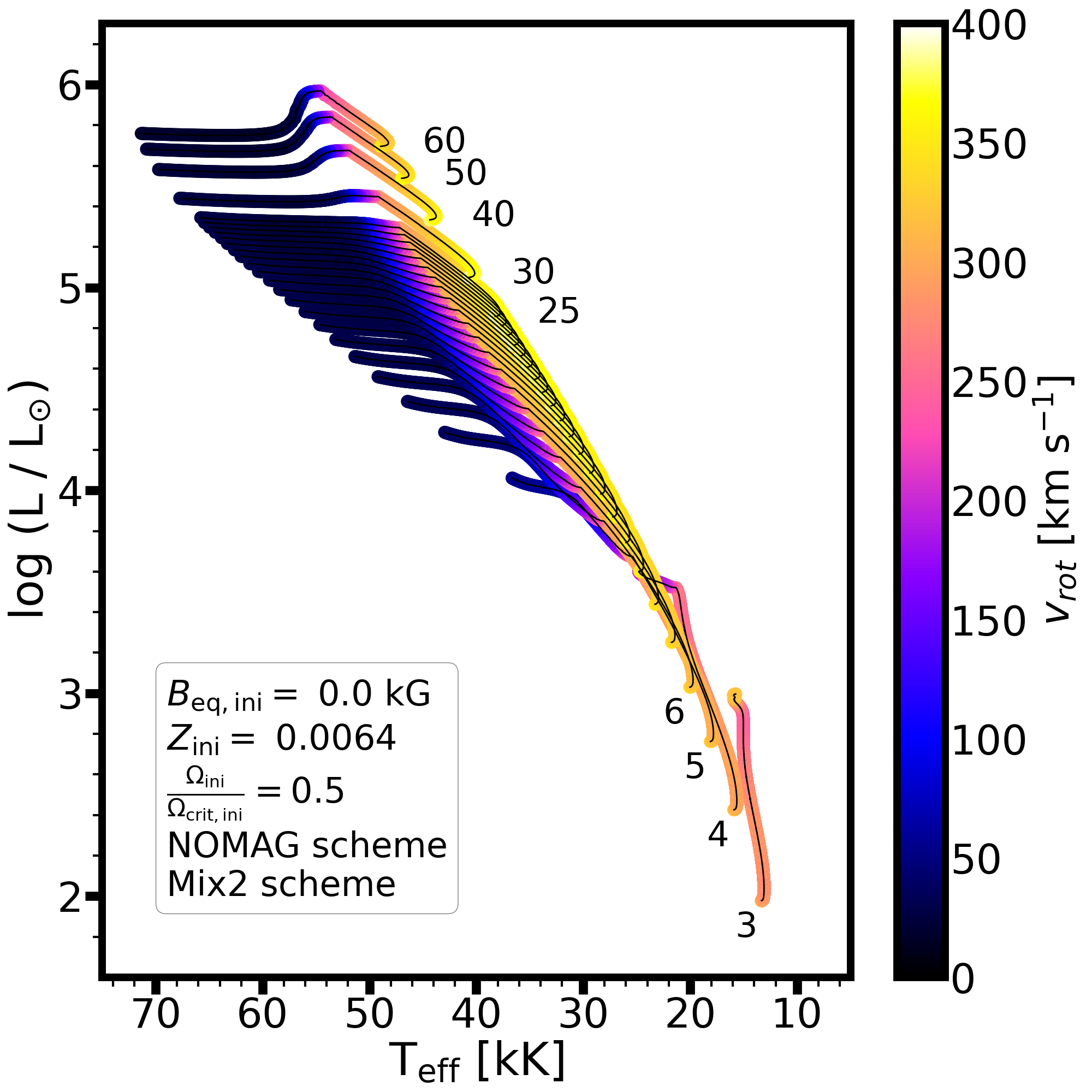
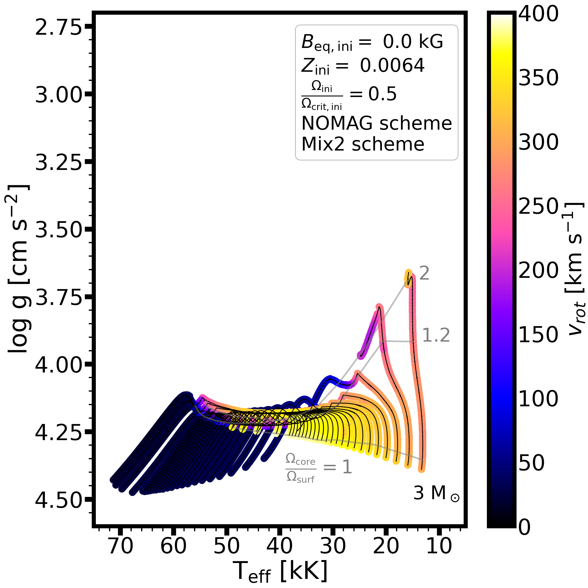
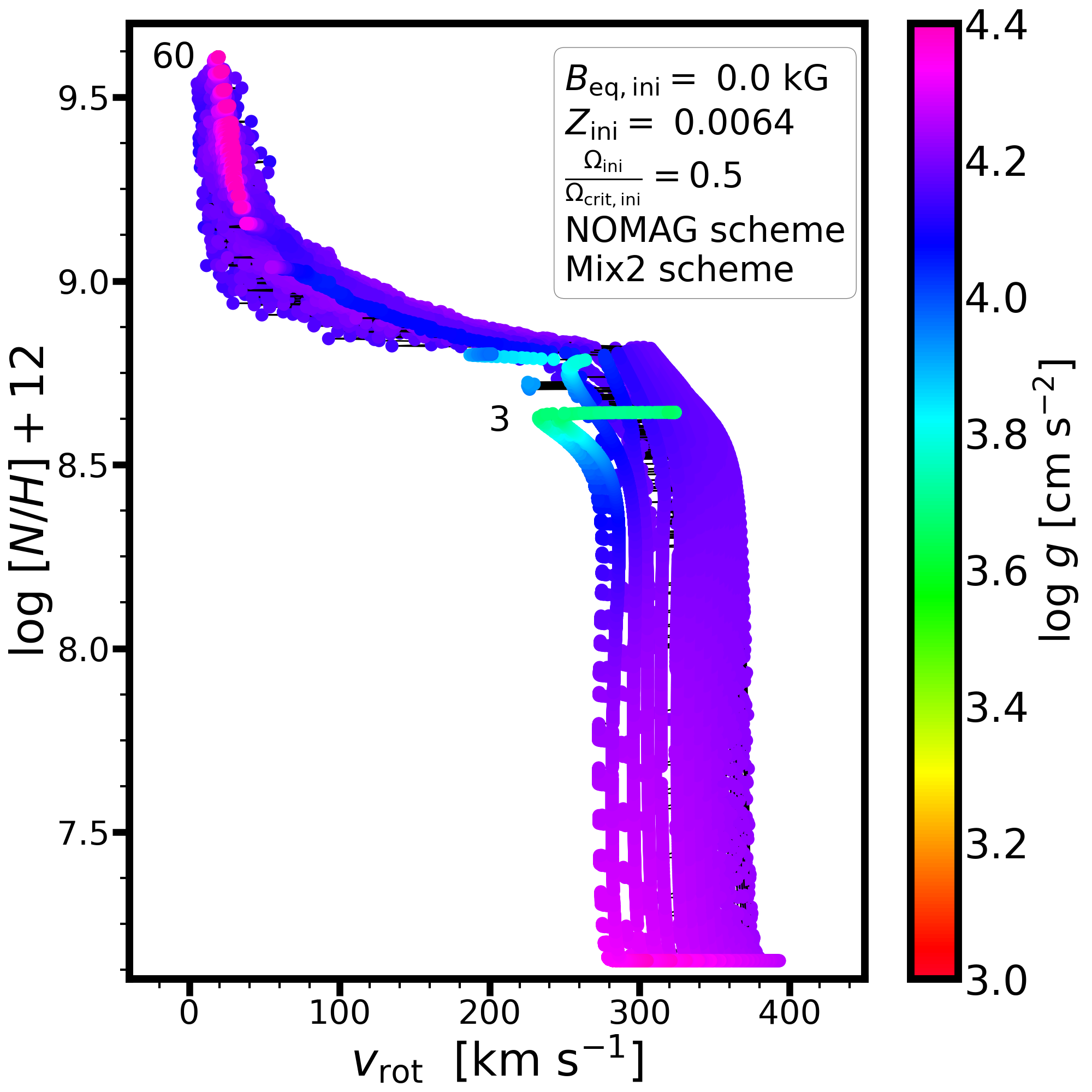
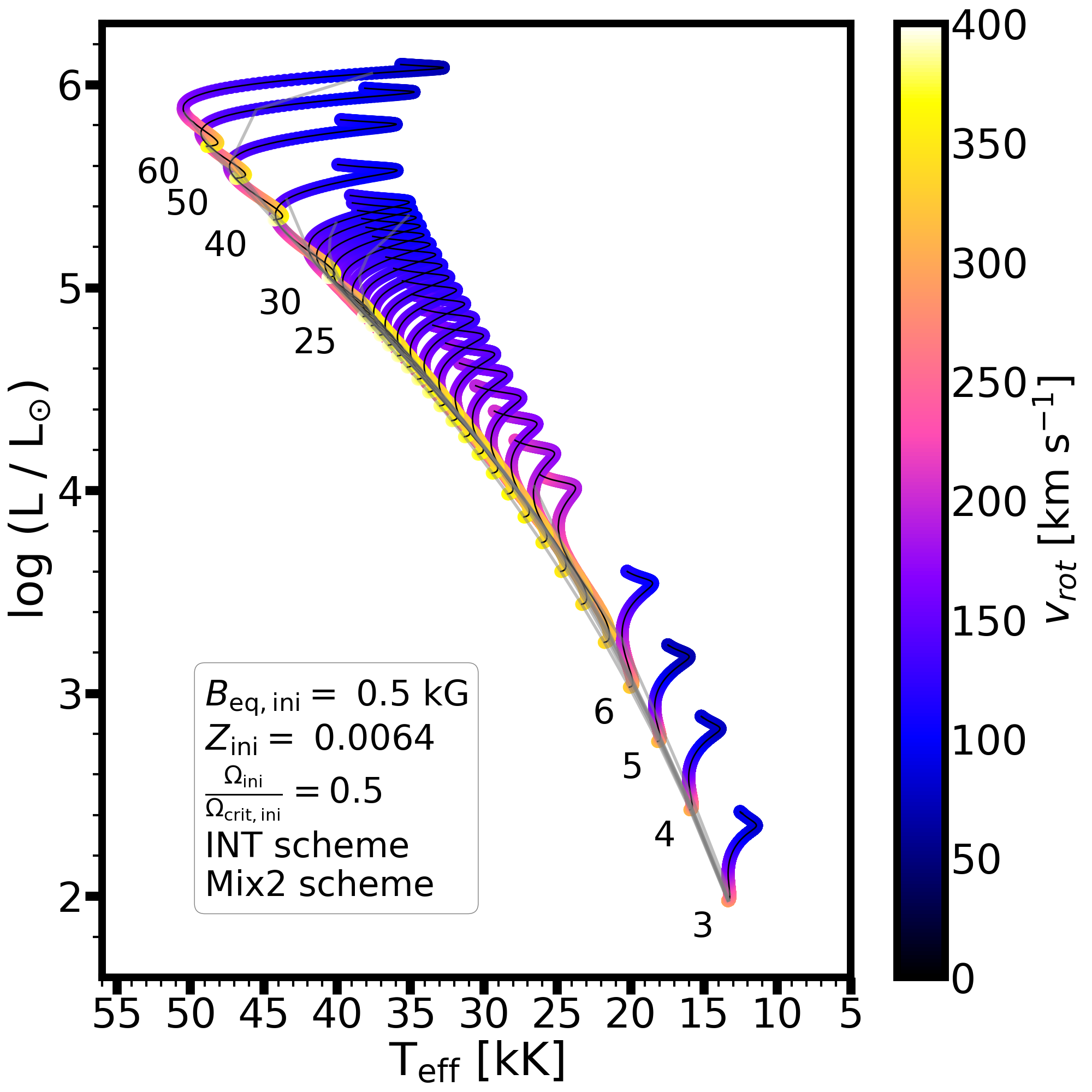
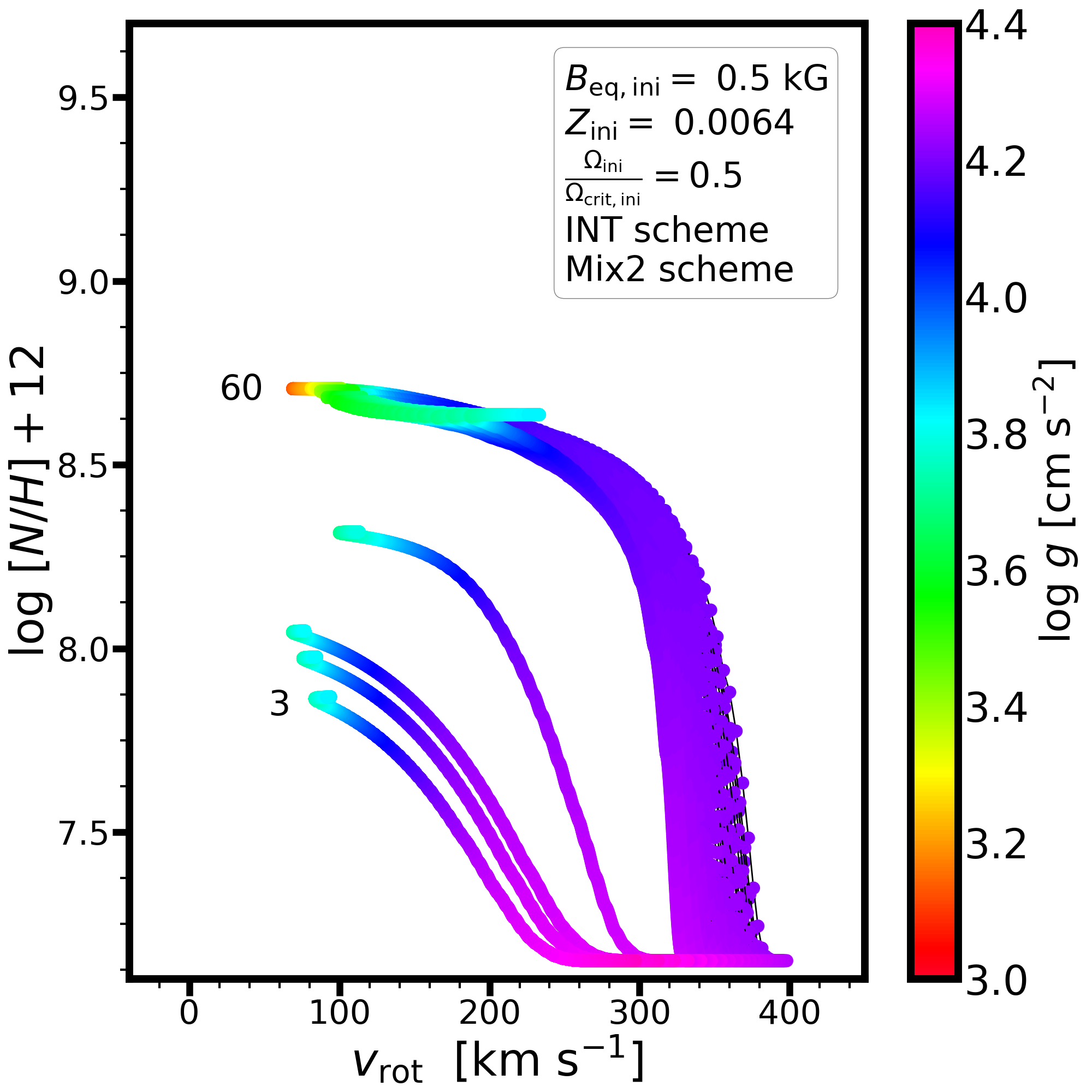
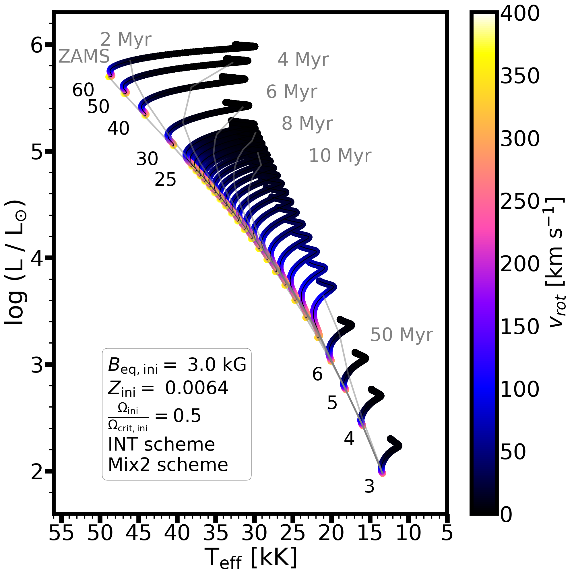
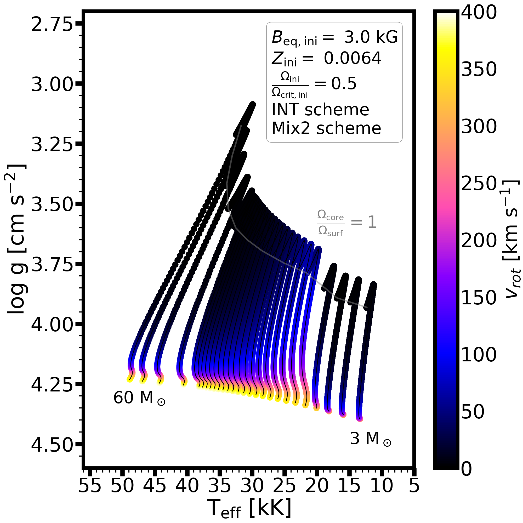
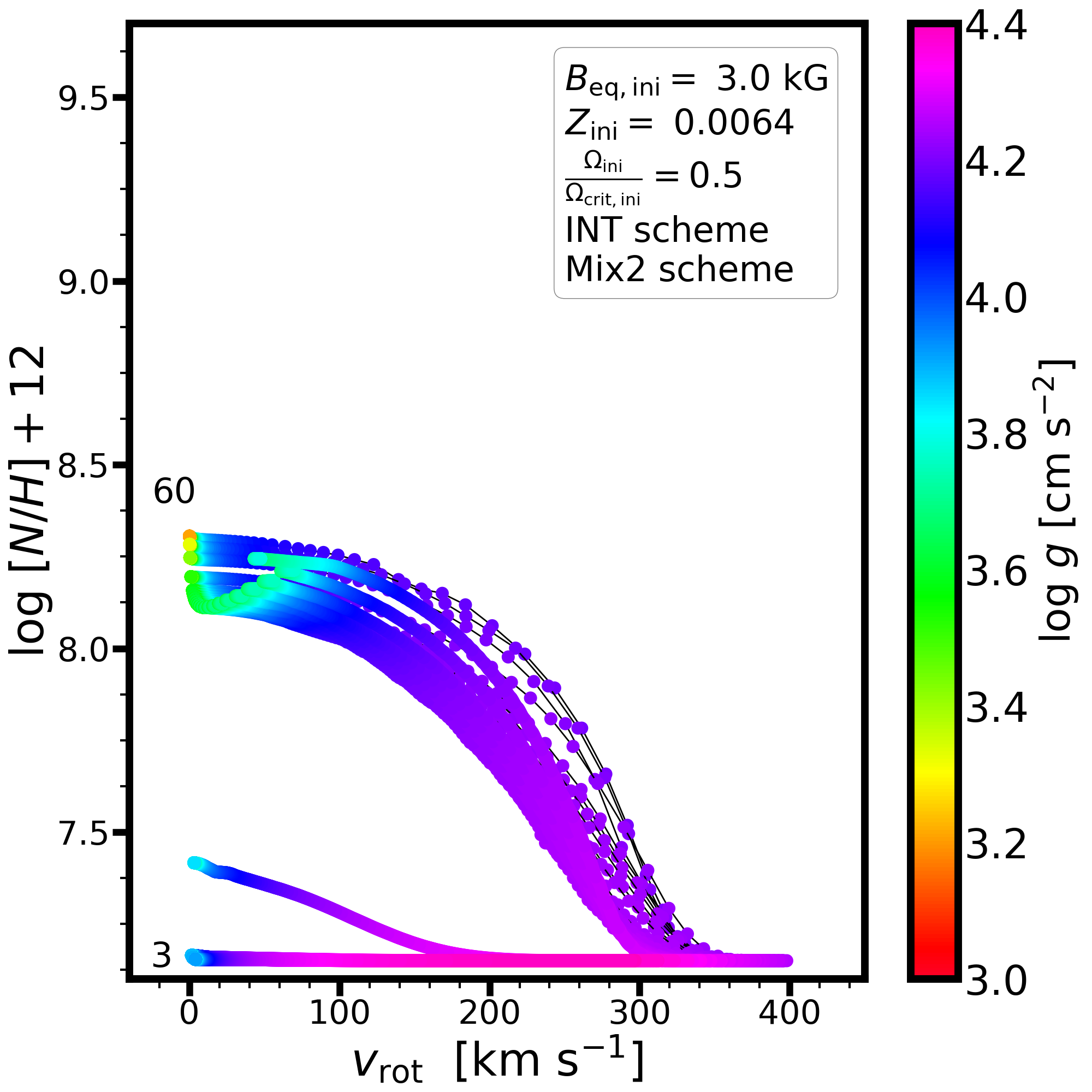
Figure 24: Same as Figure 22 but for the NOMAG/Mix2 (top panels) and INT/Mix2 (middle and lower panels) schemes.

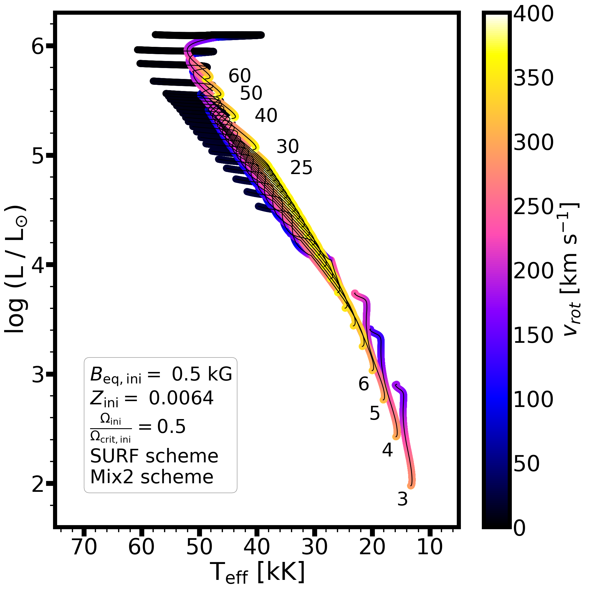
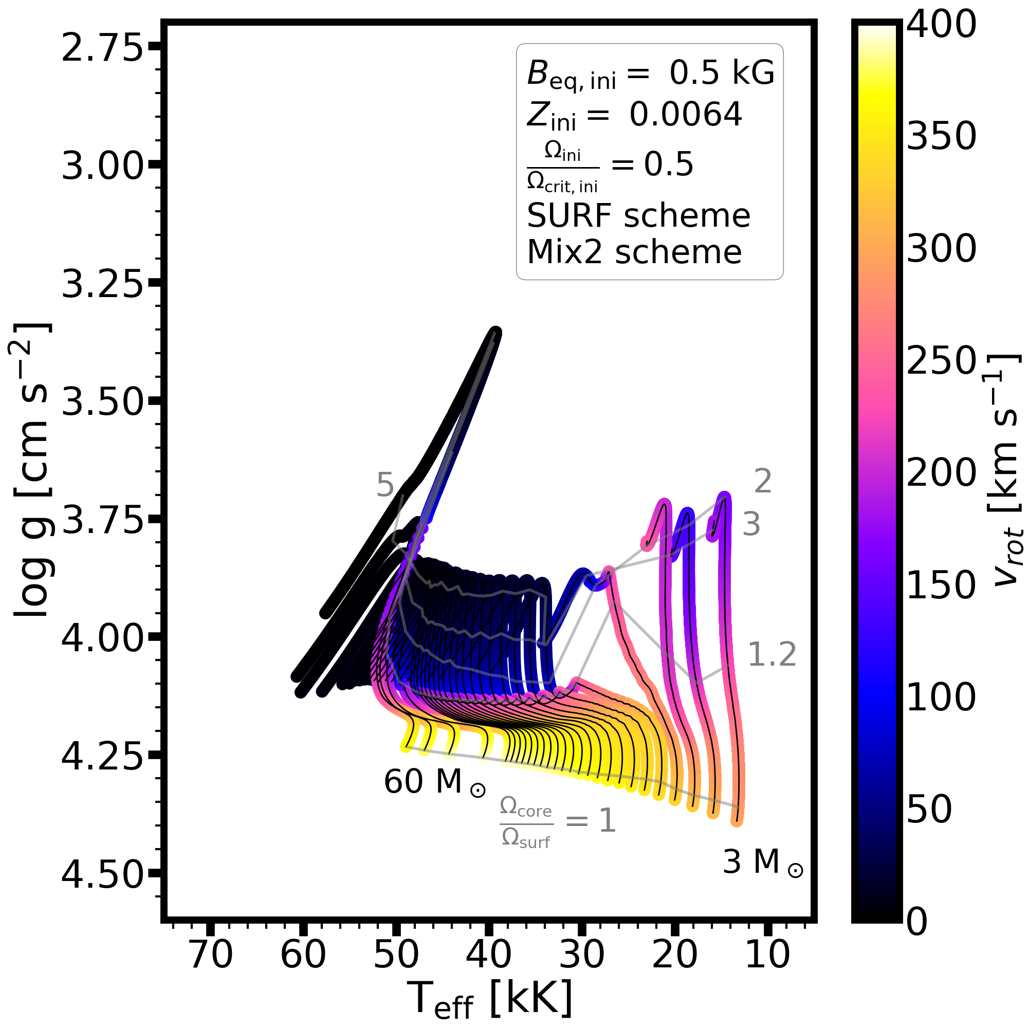
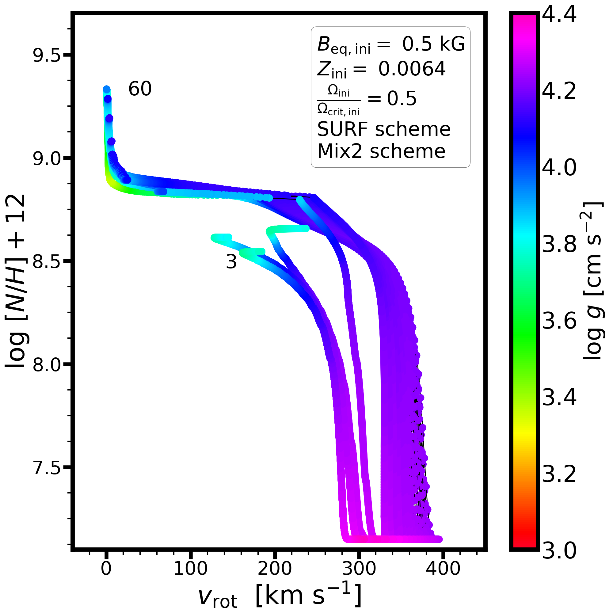
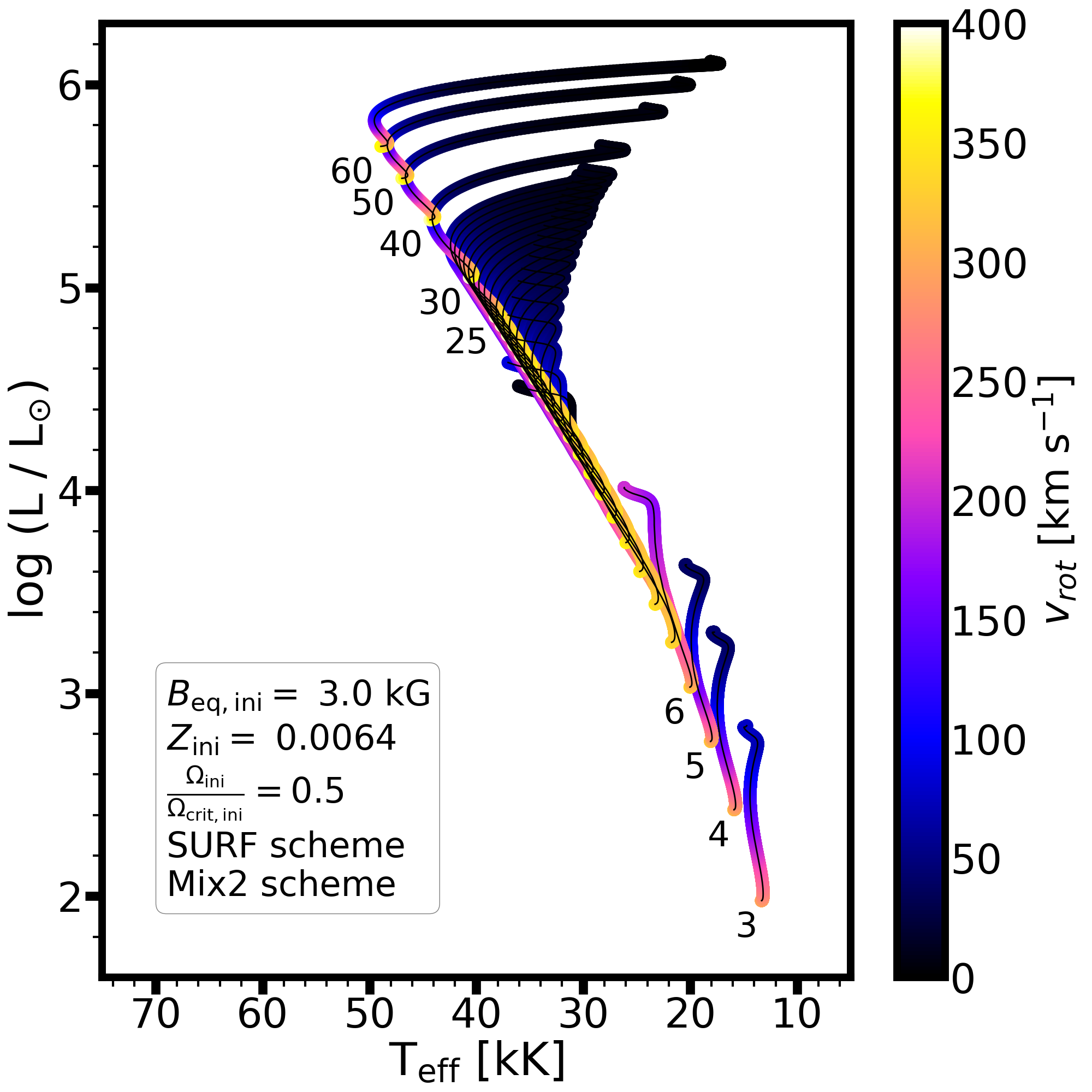
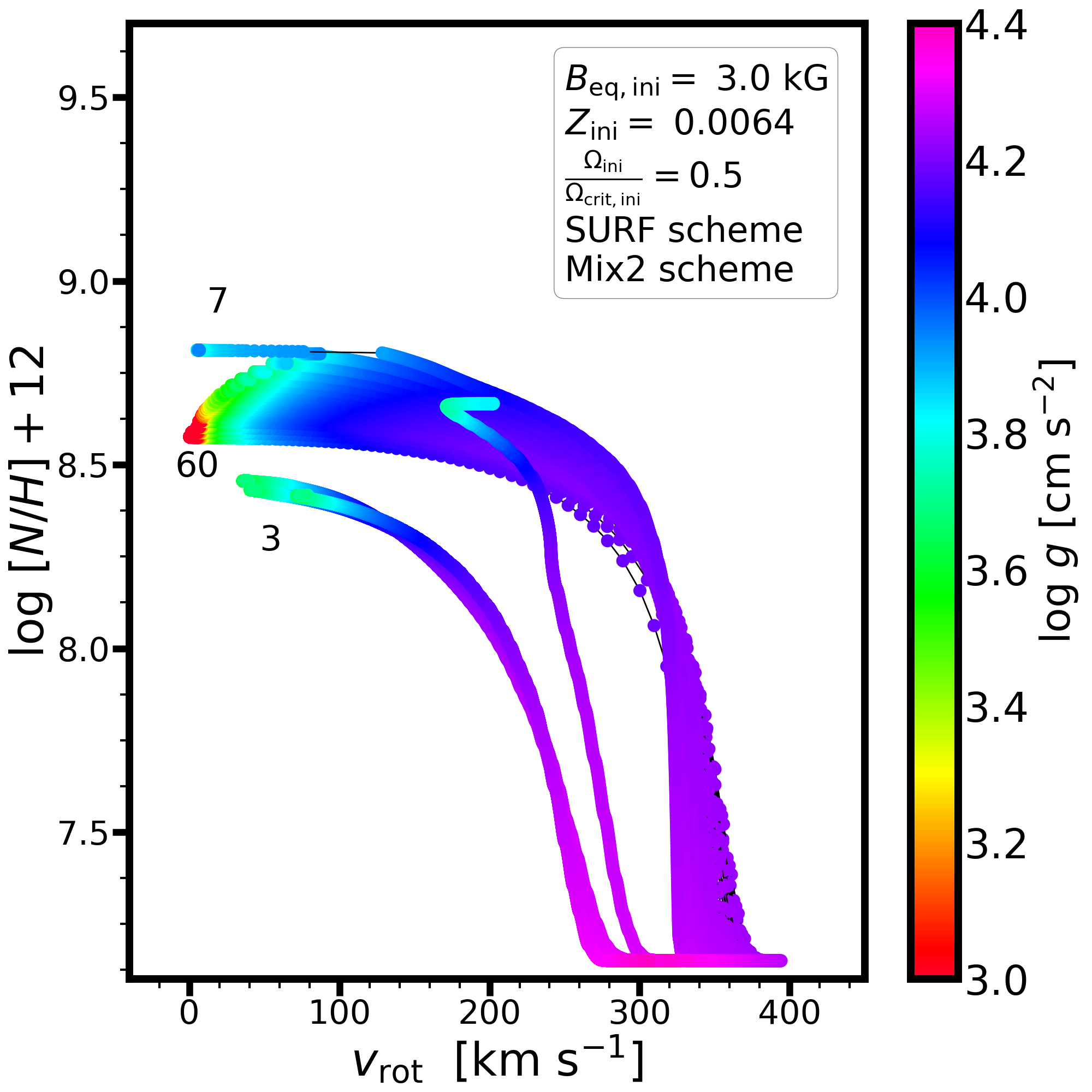
Figure 25: Same as Figure 24 but for the SURF/Mix2 scheme. See top panels of Figure 24 for the NOMAG/Mix2 models.

E.3 Impact of varying magnetic field strength at $Z=0.0064$

E.3.1 INT/Mix1

At LMC metallicity, the non-magnetic models have several main differences compared to solar metallicity models. First, at lower metallicity the position of the ZAMS is shifted to higher effective temperatures. Second, the relative amount of surface nitrogen enrichment is much higher. For comparison, the 60 M_⊙ model in the Mix1 chemical mixing scheme at solar metallicity produces an order of magnitude enrichment in its surface nitrogen to hydrogen ratio over its main sequence evolution, whereas the LMC model produces almost a factor of 30 (see Figure 22).

With a 0.5 kG initial equatorial magnetic field strength within the INT/Mix1 scheme, the surface equatorial rotational velocity is reduced in the models due to magnetic braking. This produces slight differences in the evolutionary tracks on the HR and Kiel diagrams. As a consequence of the reduced rotation in the star, chemical mixing is also somewhat less efficient compared to the non-magnetic case.

E.3.2 SURF/Mix1

With a 0.5 kG initial equatorial magnetic field strength within the SURF/Mix1 scheme (Figure 23), the overall reduction in surface equatorial rotational velocities is somewhat less than in the INT/Mix1 case. On the other hand, the most massive models in this configuration tend to achieve lower rotational velocities at the TAMS.

With a stronger, 3 kG initial equatorial magnetic field strength, the numerical simulations show that the position of the models on HR and Kiel diagram are similar to the non-magnetic and 0.5 kG cases, except for the most massive stars, which can reach much lower surface gravities towards the end of their main sequence evolution. As expected, the evolution of surface equatorial rotational velocities is also impacted, showing that a spin-down is achieved in all models. (However, see Section 3.2.4 for the discussion on models in the mass range of 8-15 M_⊙.) Consequently, the surface nitrogen enrichment is more modest compared to the non-magnetic case but still notable in these models.

E.3.3 INT/Mix2

When chemical mixing is assumed in the Mix2 scheme, the non-magnetic models at LMC metallicity evolve bluewards, quasi-chemically homogeneously for their entire main sequence evolution. Within this configuration the $[N/H]$ ratio reaches extremely high values (Figure 24). This is in part due to the efficient mixing of nitrogen, and in part due to losing a significant amount of hydrogen from the stellar surface via winds. In this case, the low surface rotational velocities at the TAMS are achieved due to Wolf-Rayet type mass loss taking away angular momentum from the star.

When a 0.5 kG initial equatorial magnetic field strength is considered within the INT/Mix2 scheme the models return to a redward evolution on the main sequence following a rapid blueward evolution. This is because the spin-down due to magnetic braking reduces the overall efficiency of chemical mixing and prevents a quasi-chemically homogeneous evolution for the entire main sequence. Note that in this case the TAMS surface rotational velocities are actually higher than in the non-magnetic case as magnetic braking weakens over time and stellar winds are less efficient compared to the non-magnetic case.

With a 3 kG initial equatorial magnetic field strength, the main differences result from a stronger magnetic braking. This almost immediately prevents a blueward evolution, producing slowly-rotating tracks in which the surface nitrogen enrichment is significantly reduced compared to the non-magnetic case.

E.3.4 SURF/Mix2

In the SURF/Mix2 scheme both set of models with 0.5 and 3 kG initial equatorial magnetic field strength undergo a rapid initial blueward evolution as in the INT/Mix2 case (Figure 25). With weaker initial magnetic fields, the models above 1̃0 M_⊙ turn to a short redward evolution before spinning down and reaching their TAMS again at hotter effective temperatures. With stronger initial magnetic fields, the spin-down leads to preventing the models from turning back to a blueward evolution by the end of their main sequence. Similarly to the SURF/Mix1 case, the most massive models with 3 kG initial equatorial magnetic field strength may reach low surface gravities. In this configuration, it is also possible that the most massive models produce a final $[N/H]$ ratio that is lower than that of lower mass models (see also Figure 11). However, given the very efficient Mix2 scheme, the predicted surface nitrogen enrichment is still expected to be observable as it is over an order of magnitude compared to the baseline.

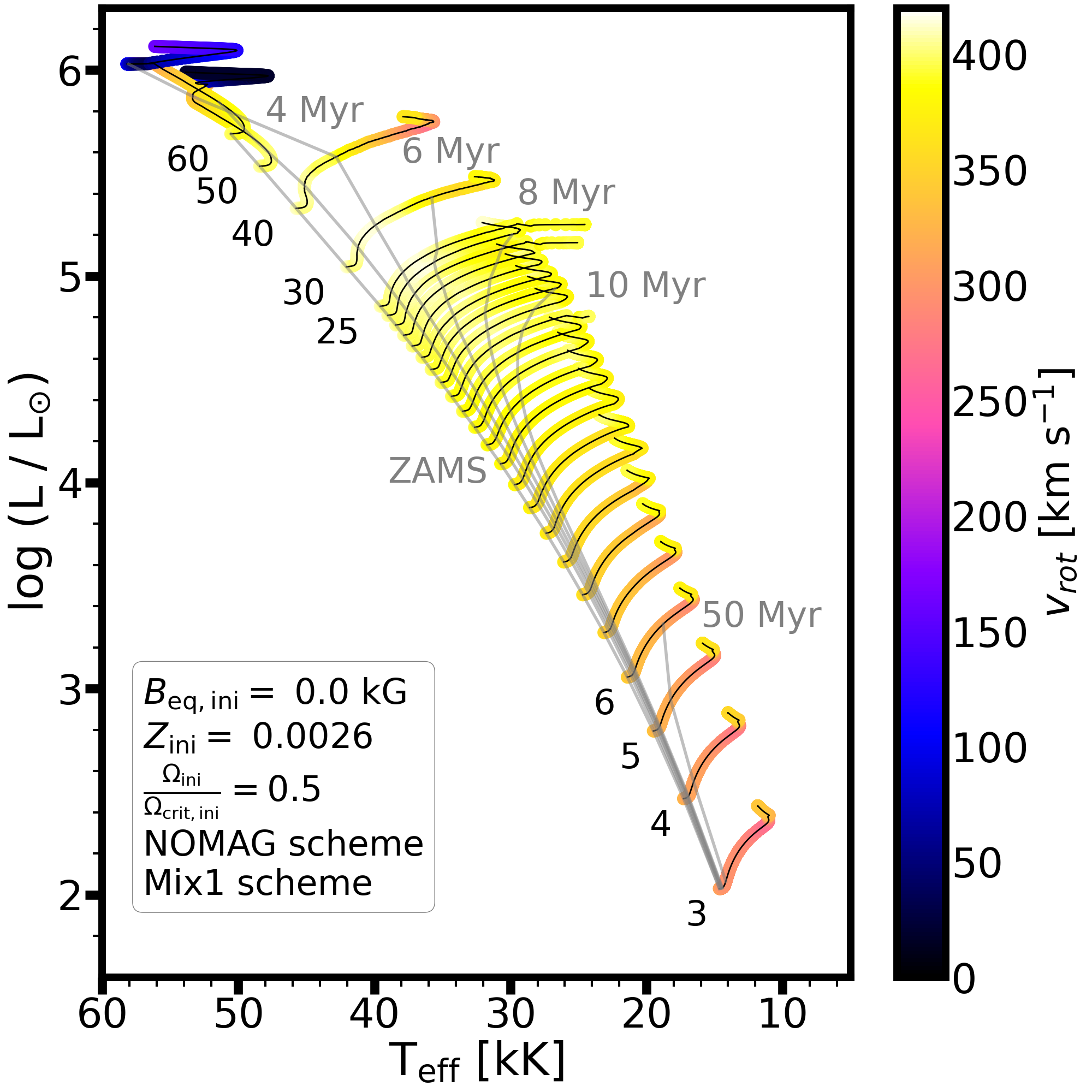
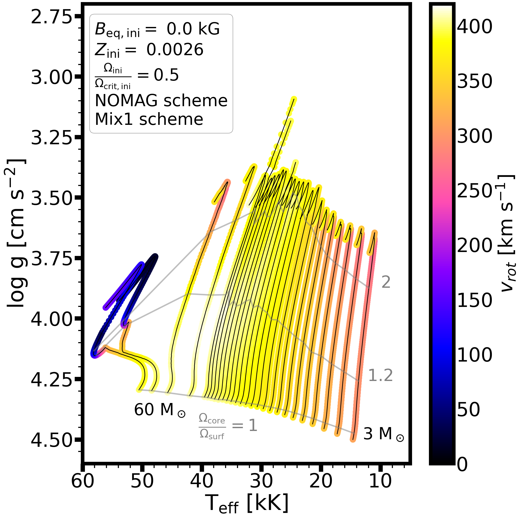
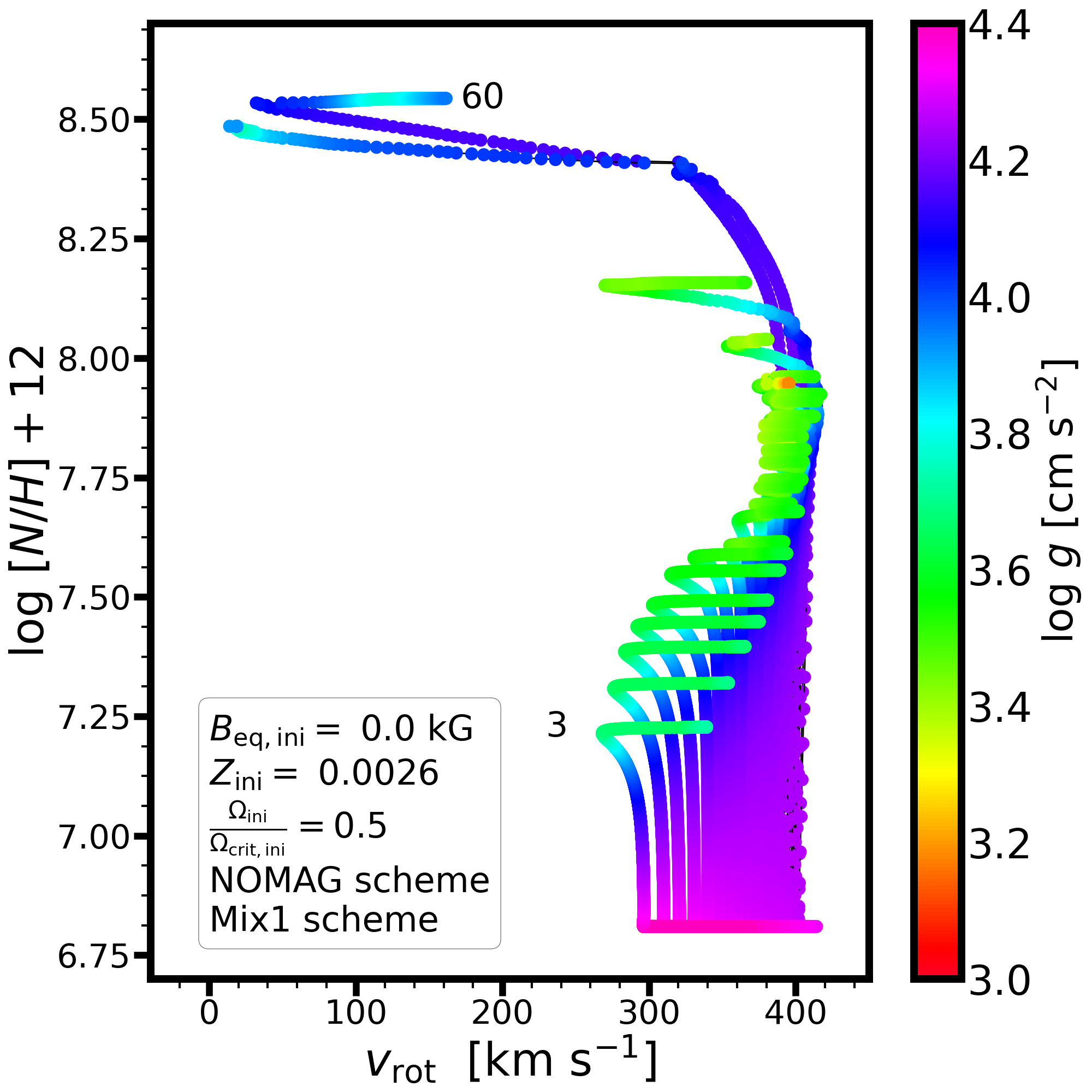
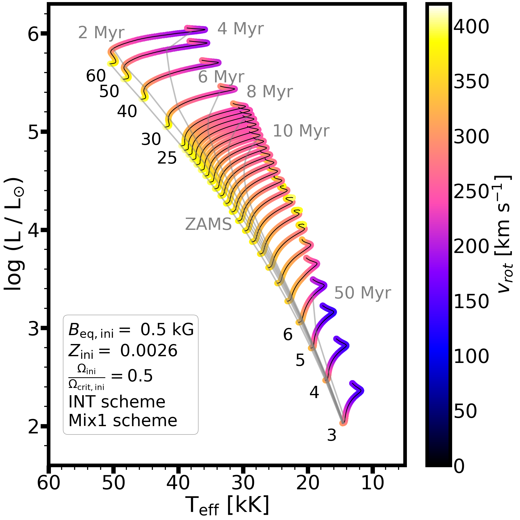
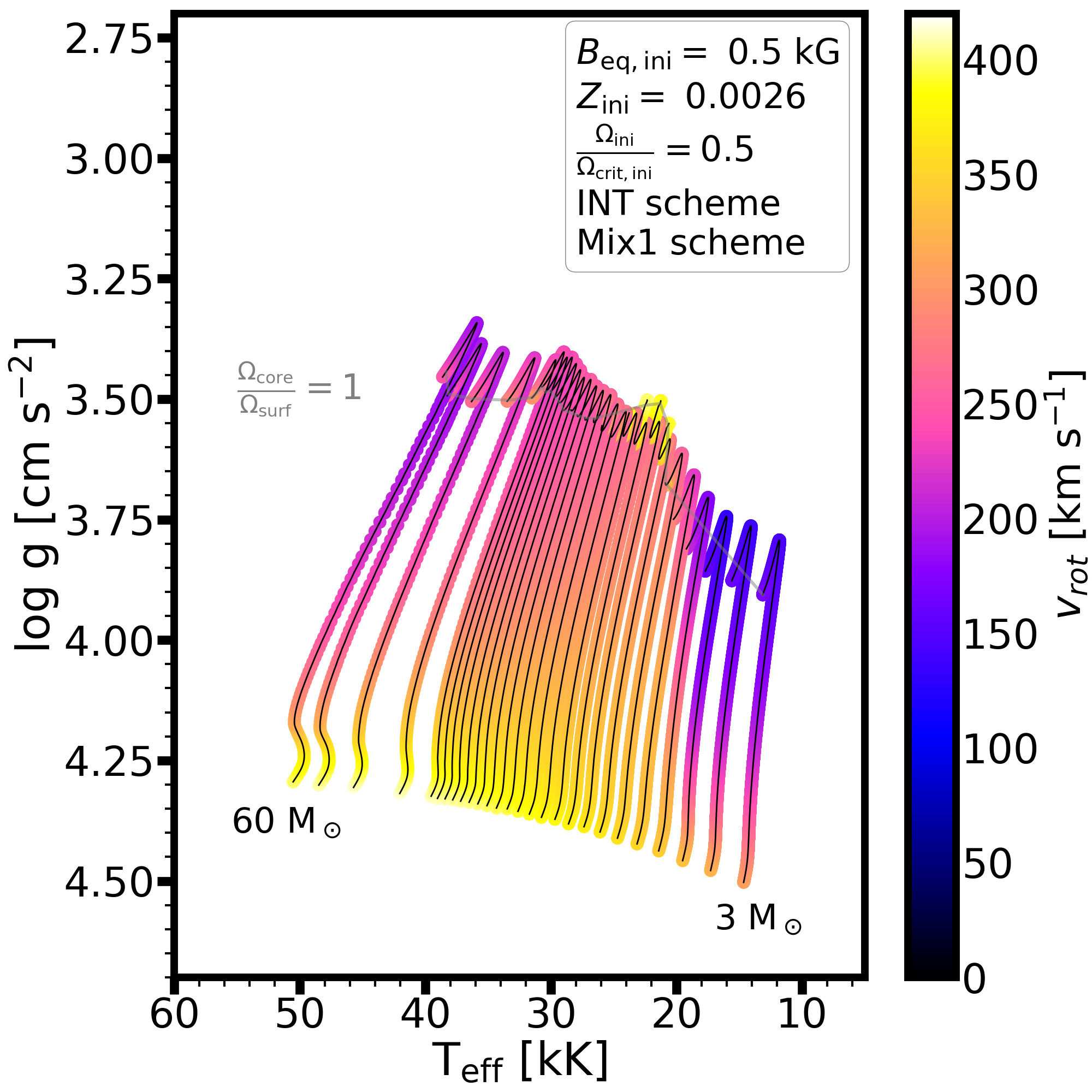
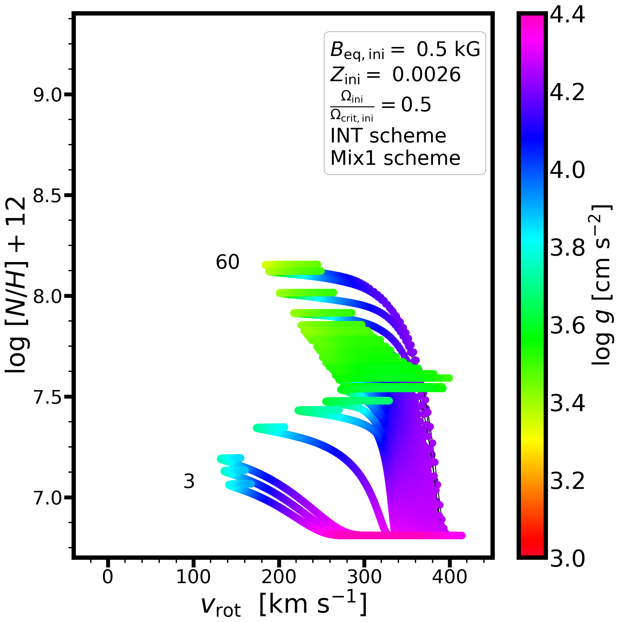
Figure 26: Same as Figure 10 but for the NOMAG/Mix1 scheme (top) and INT/Mix1 scheme with an initial equatorial magnetic field strength of 0.5 kG (lower panel) at $Z=0.0026$. The INT/Mix1 model with initial equatorial magnetic field strength of 3 kG is presented in Figure 10.

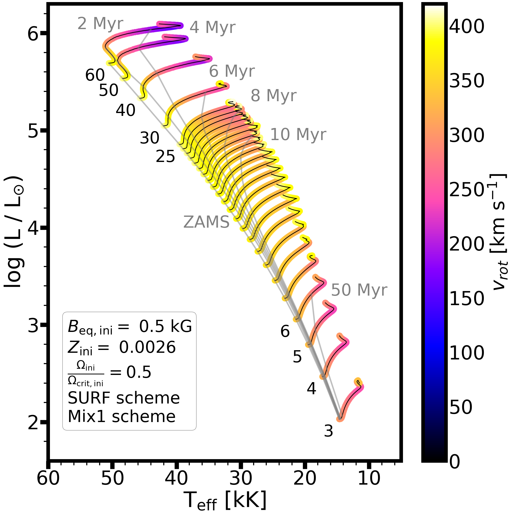
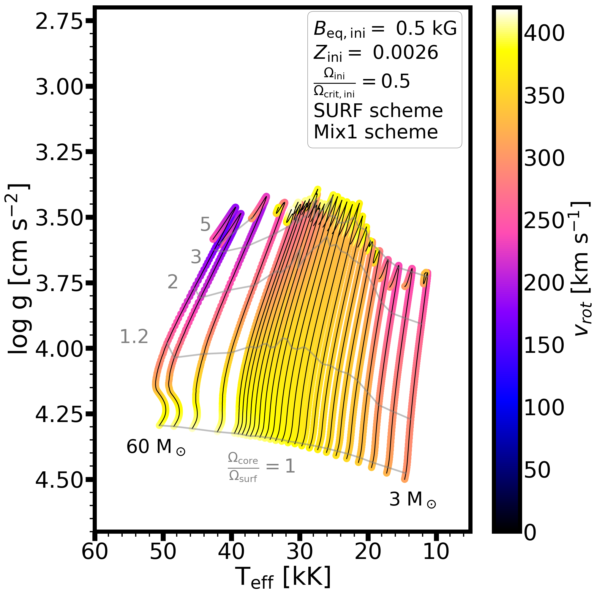
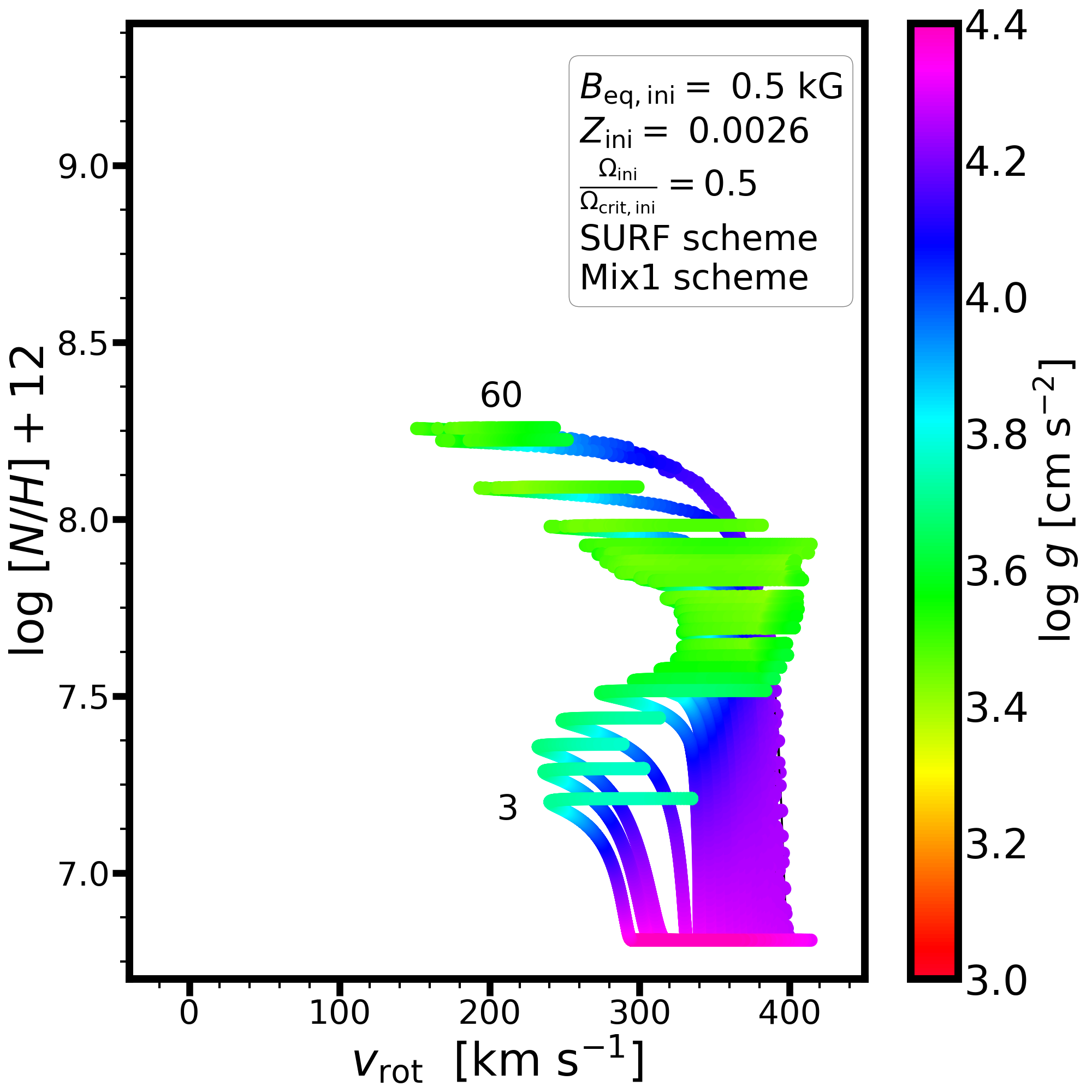
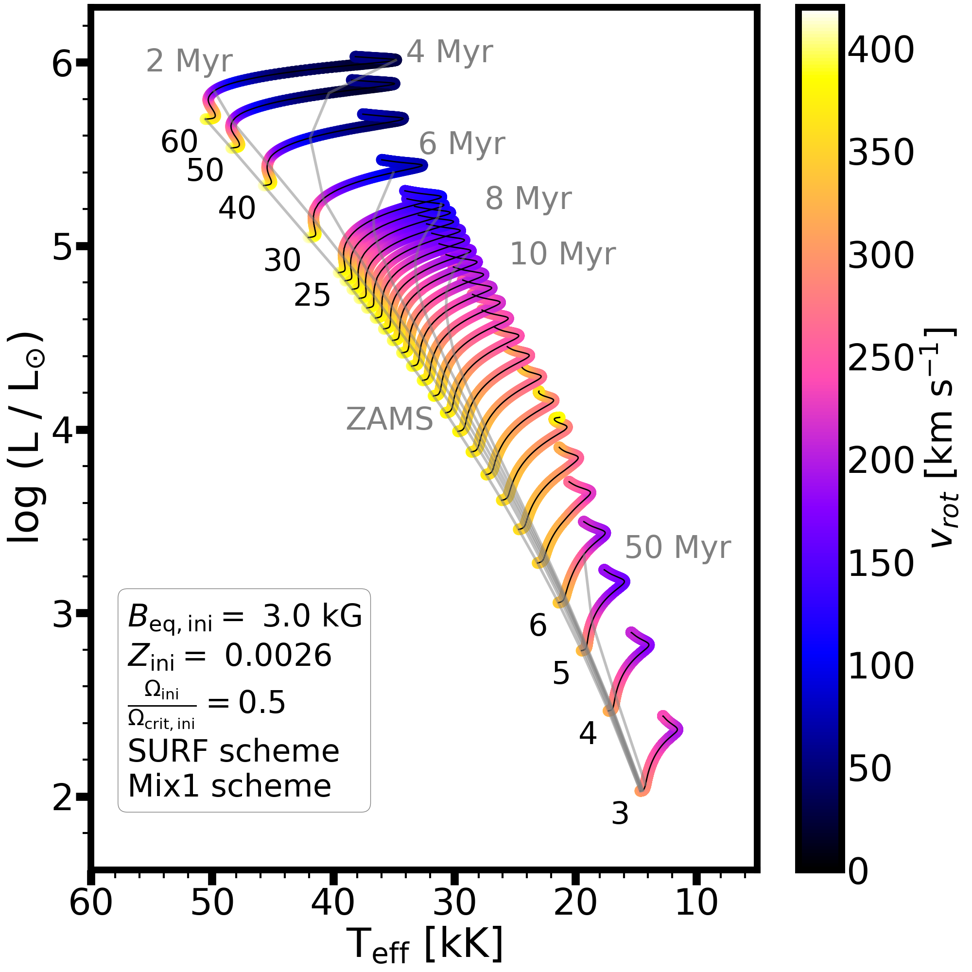
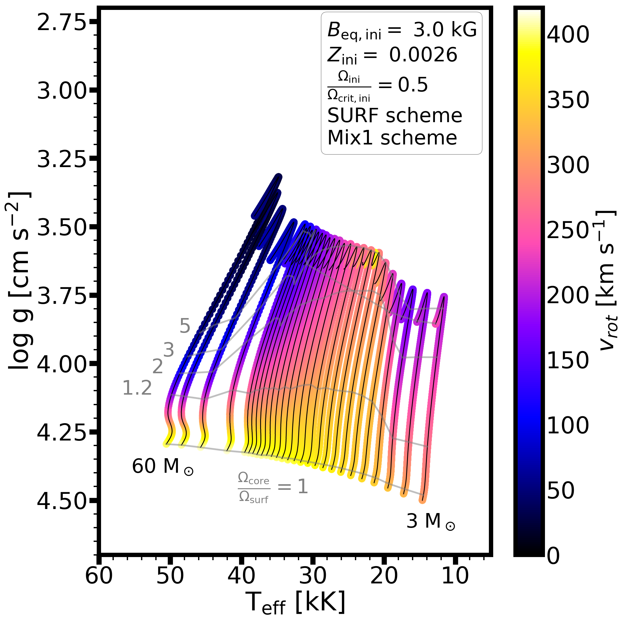
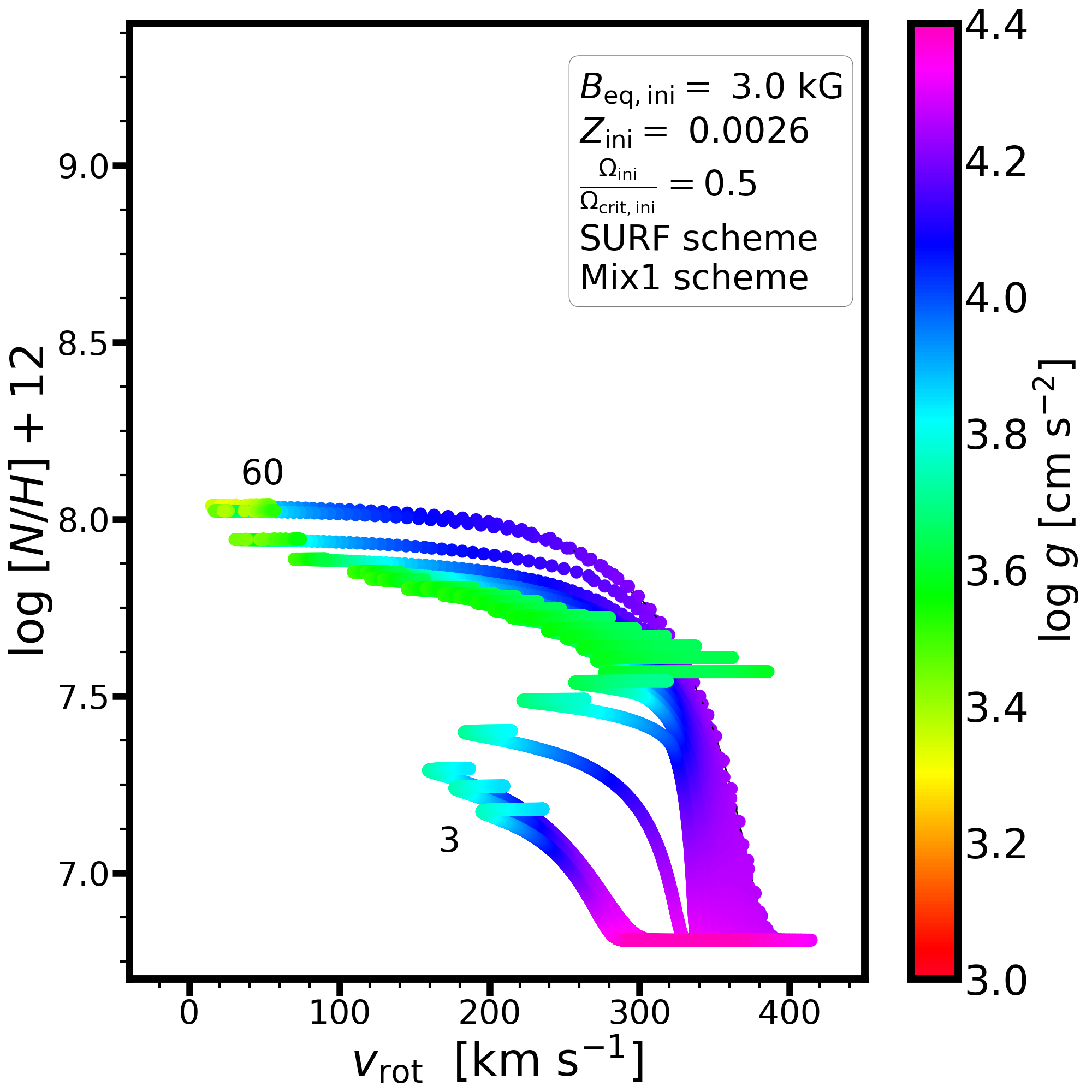
Figure 27: Same as Figure 26 but for the SURF/Mix1 scheme. Top panels show models with an initial equatorial magnetic field strength of 0.5 kG, whereas the lower panels show models with 3 kG. The NOMAG/Mix1 model is presented in Figure 26.

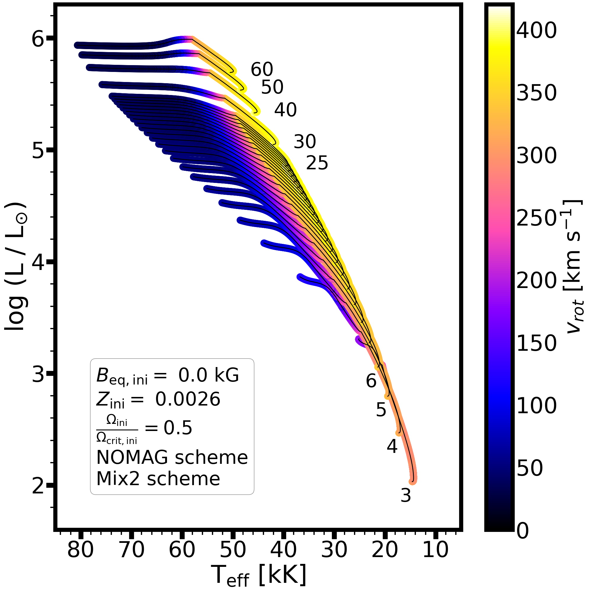
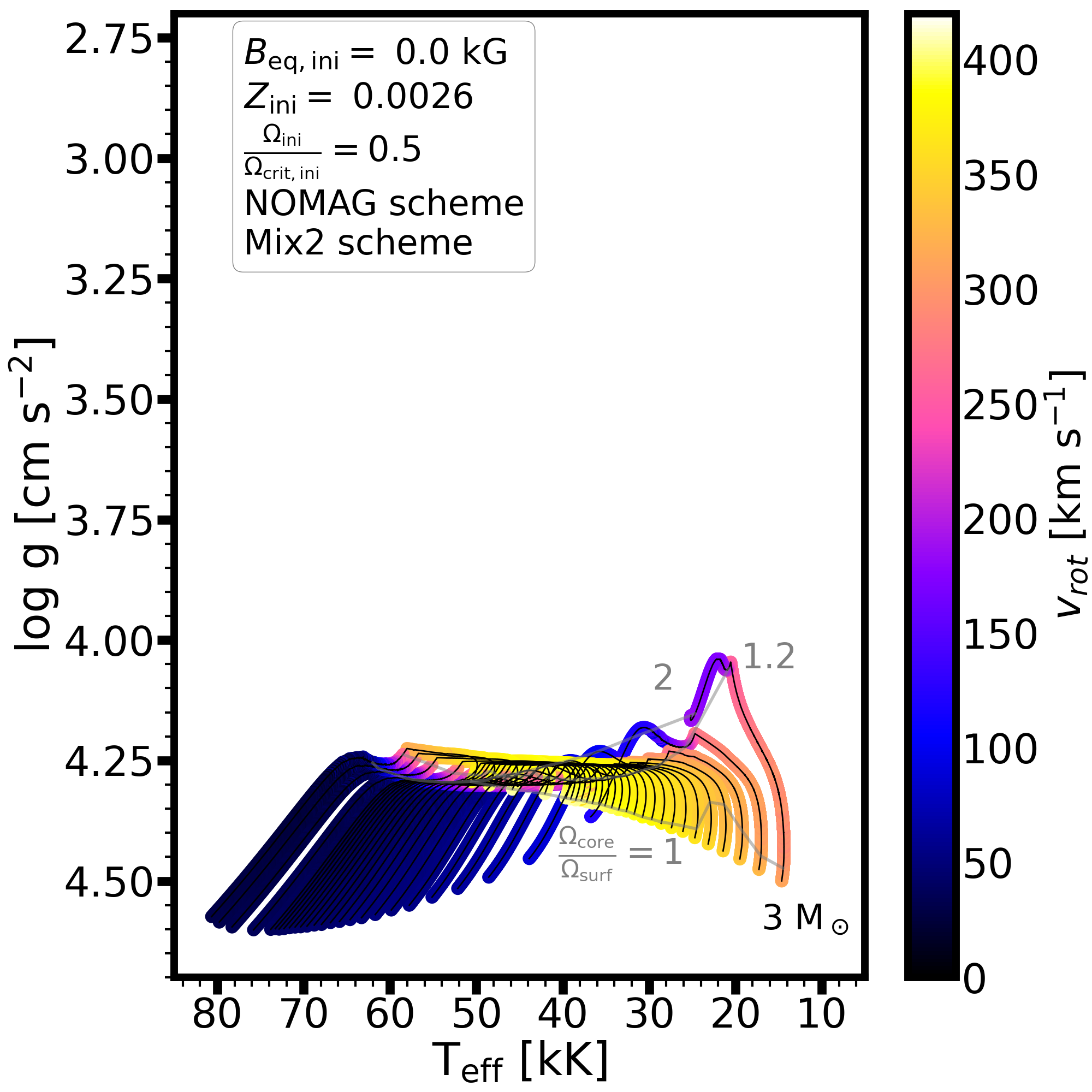
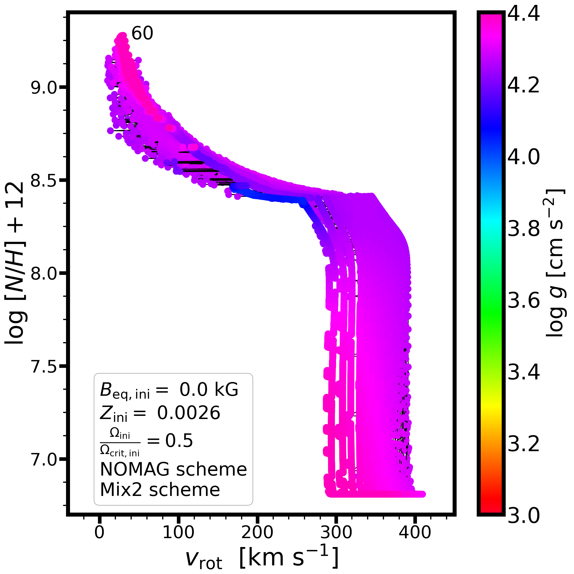
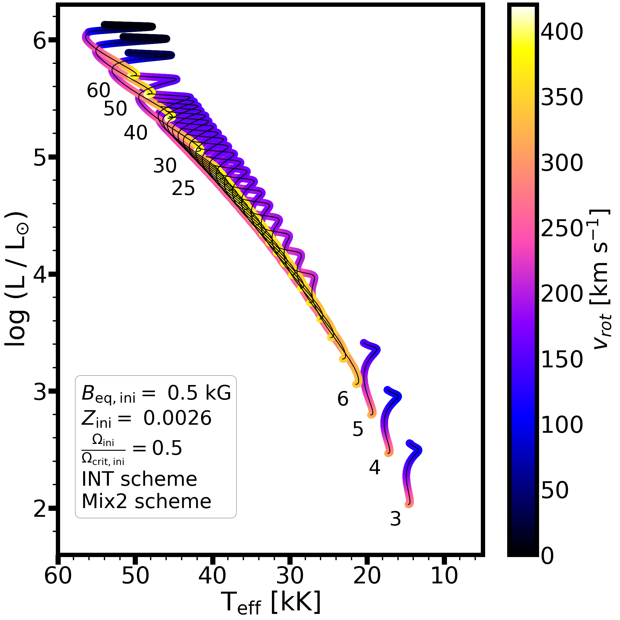
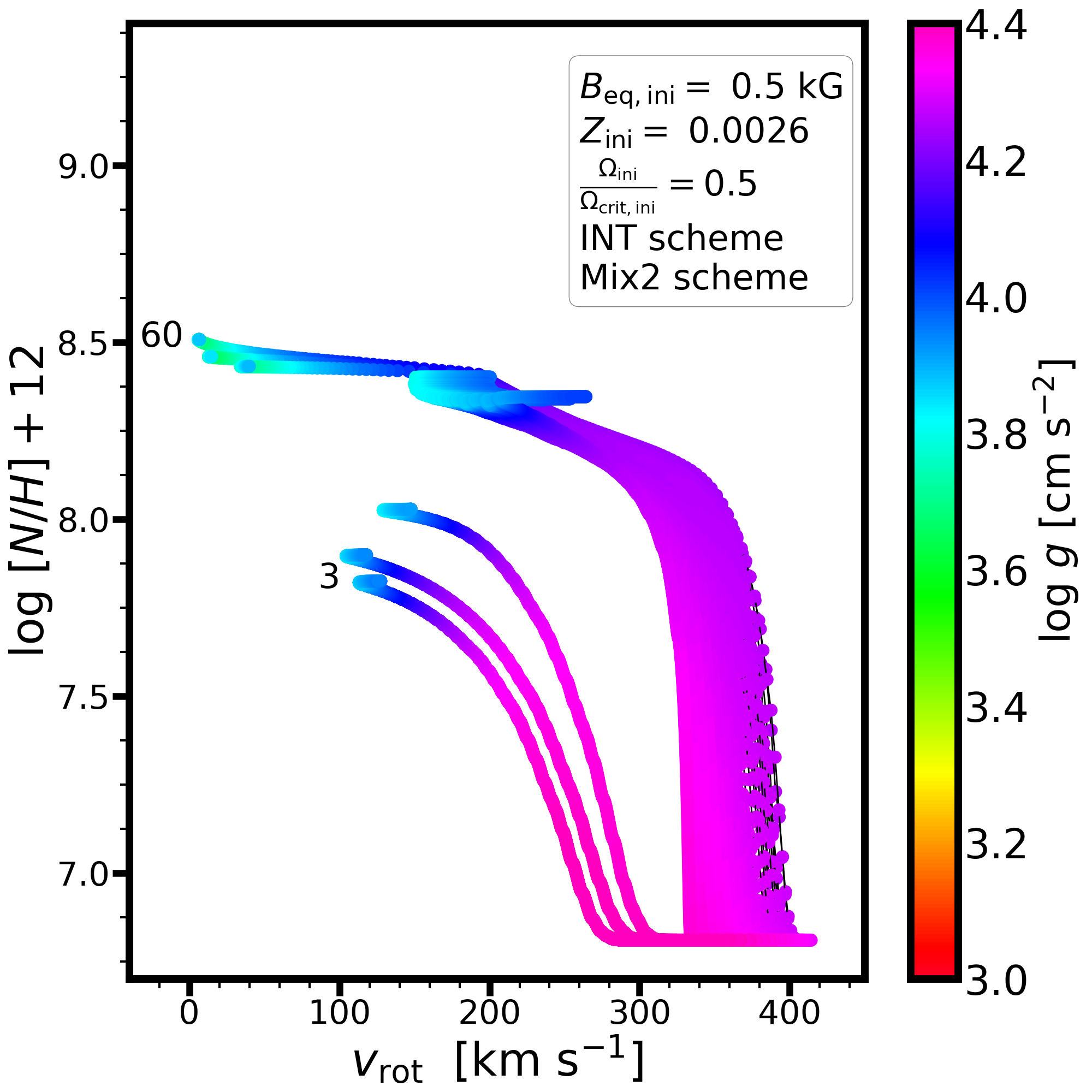
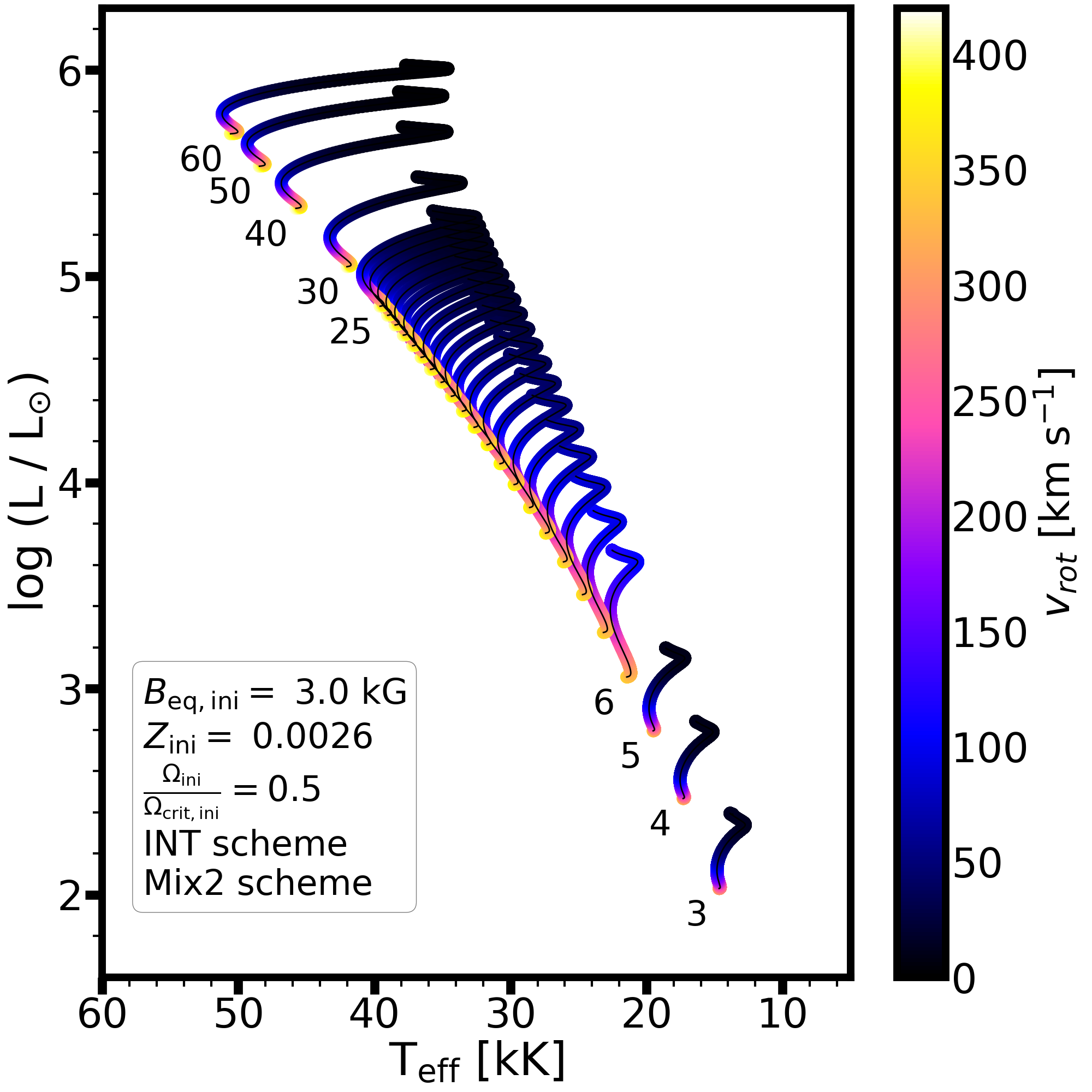
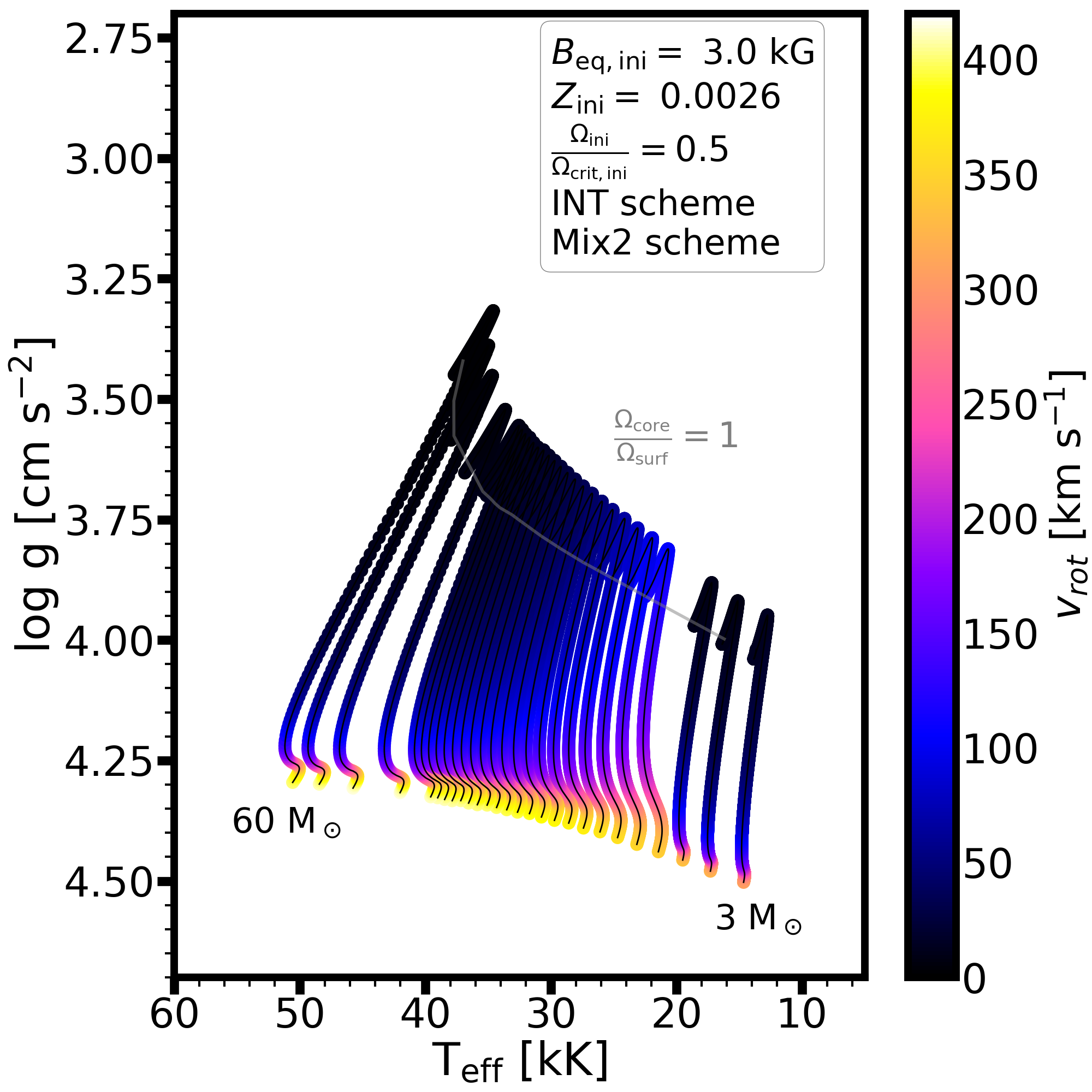
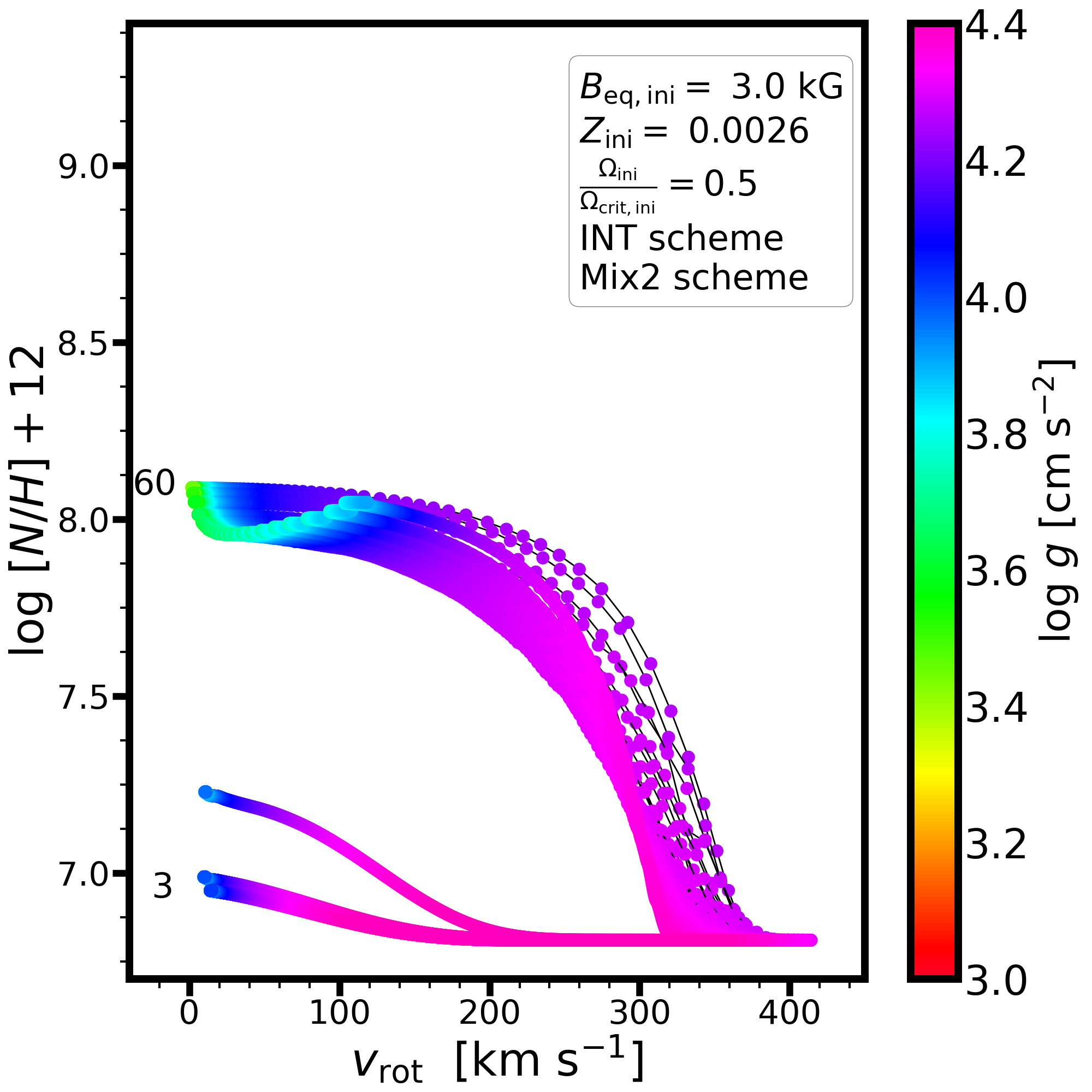
Figure 28: Same as Figure 26 but for the NOMAG/Mix2 (top panels) and INT/Mix2 (middle and lower panels) schemes.

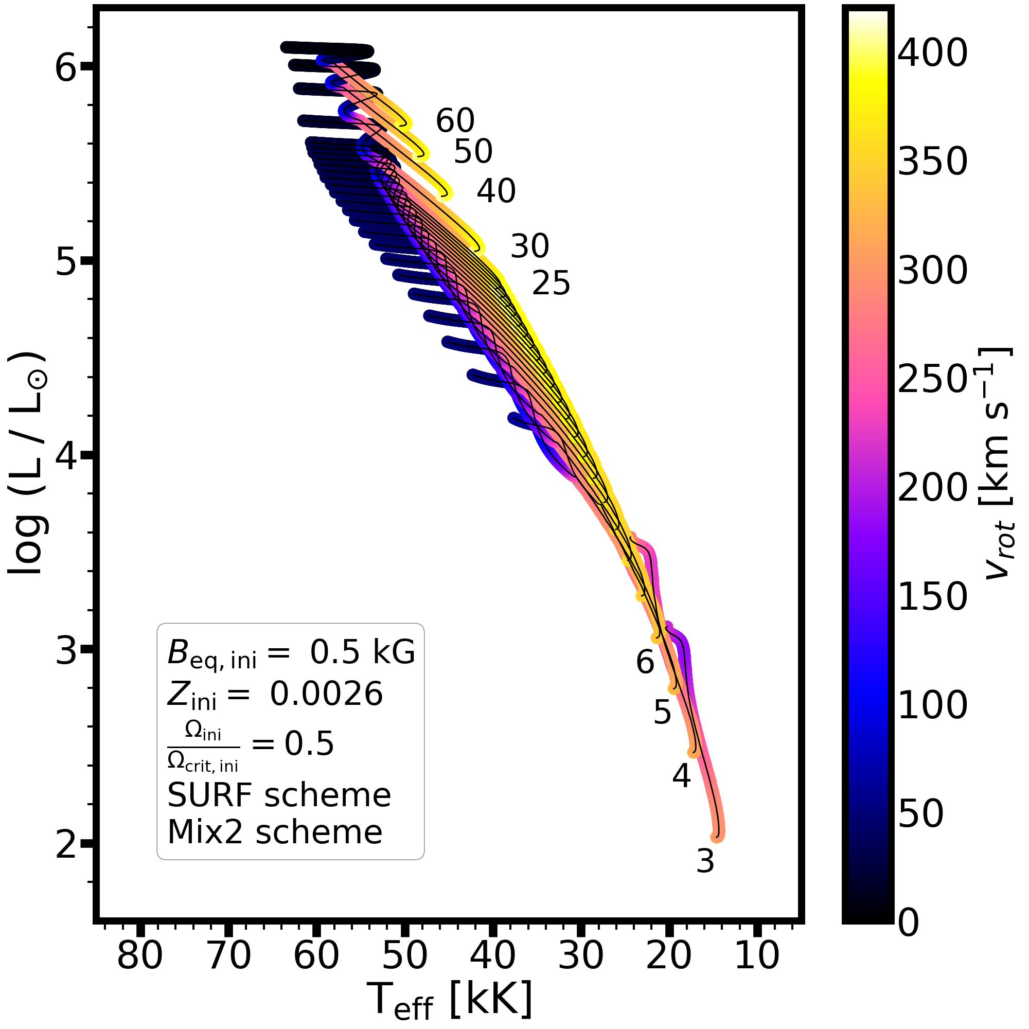
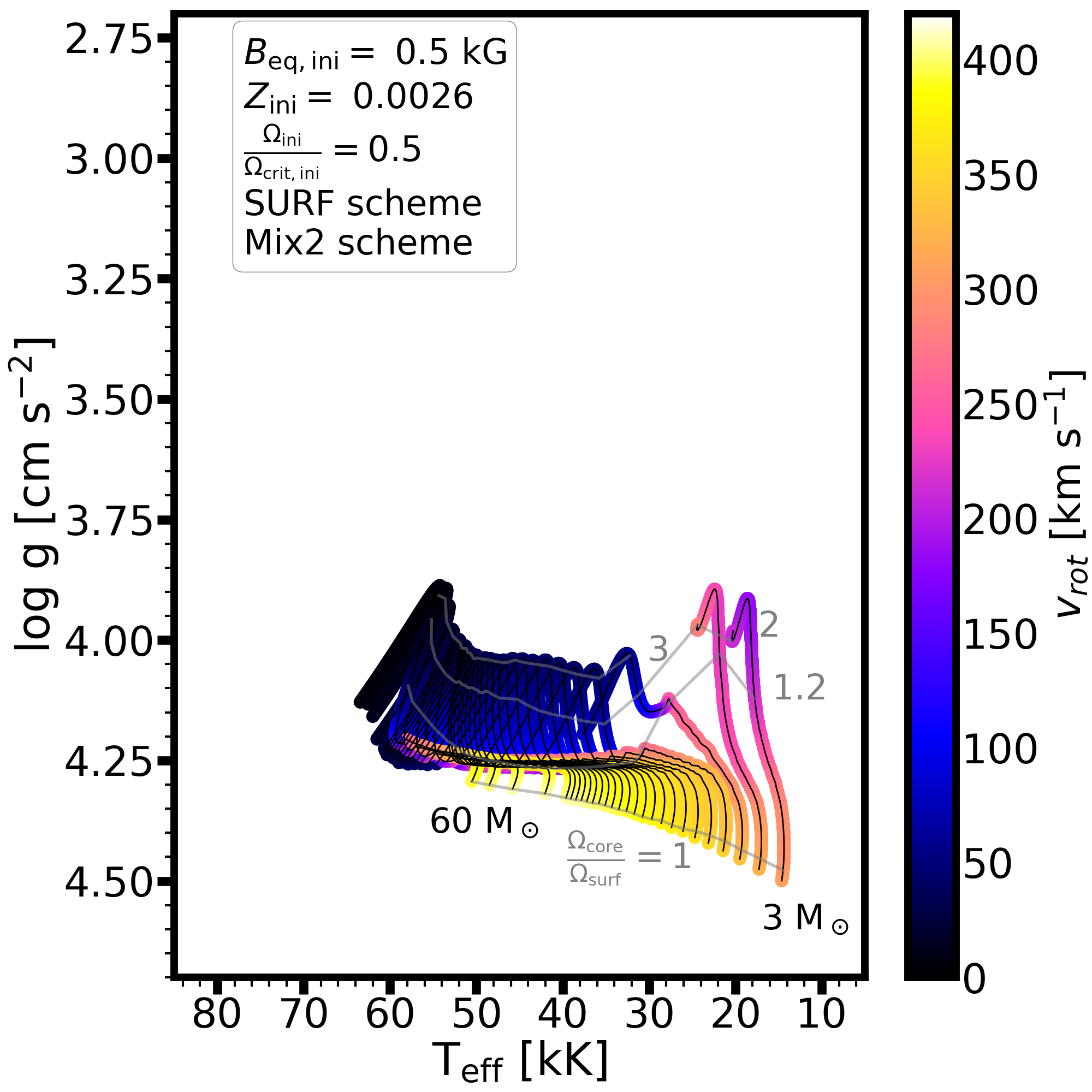
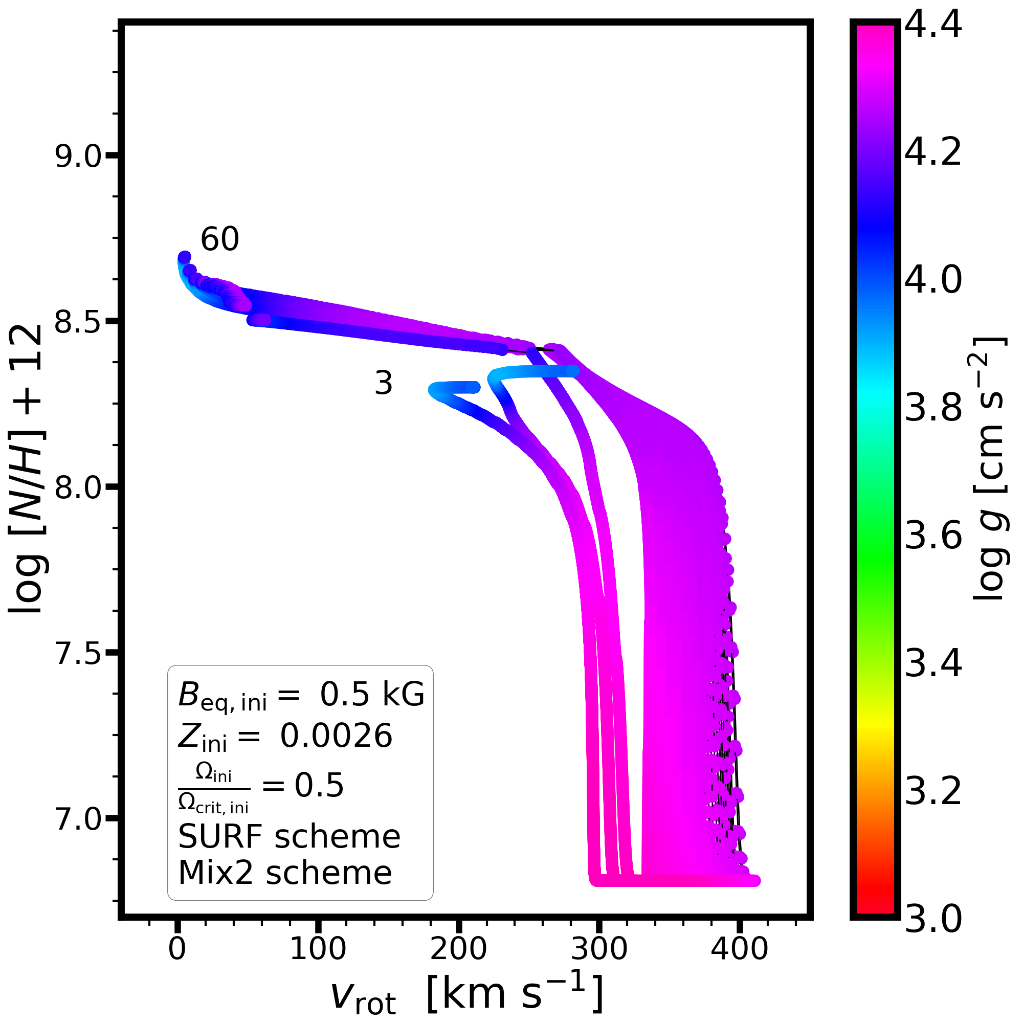
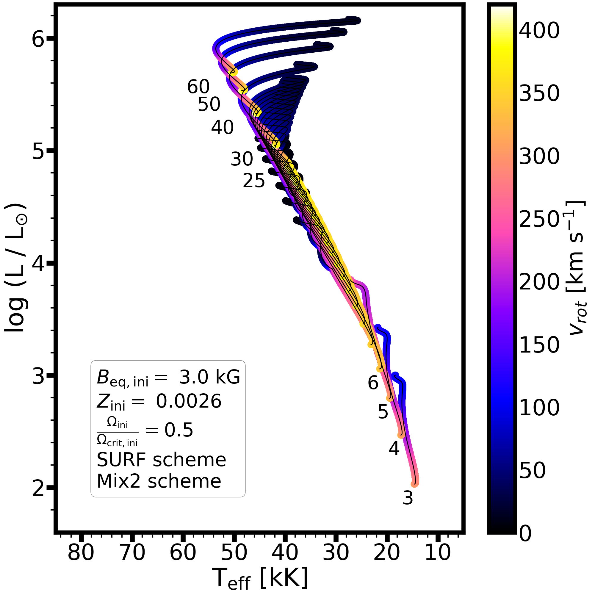
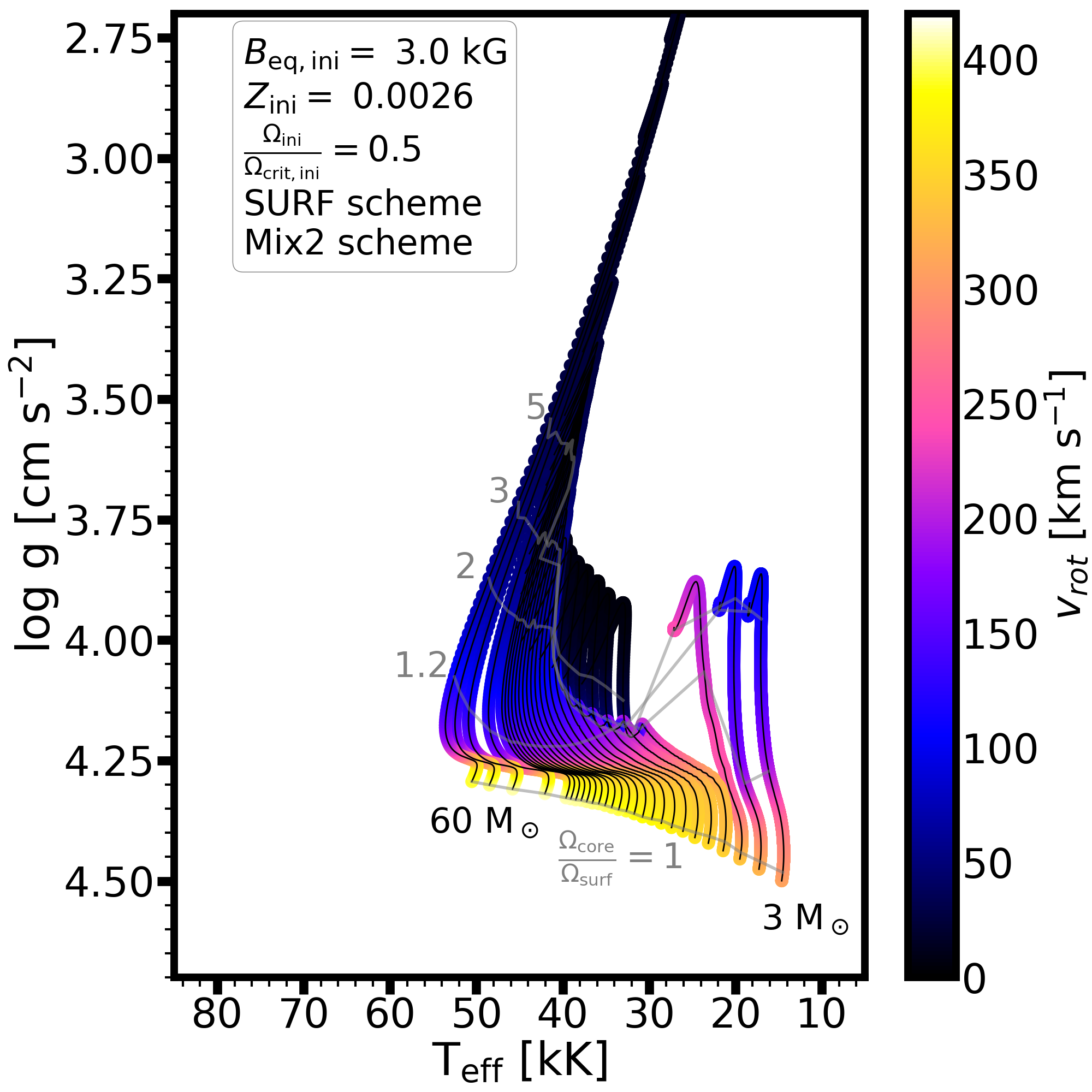
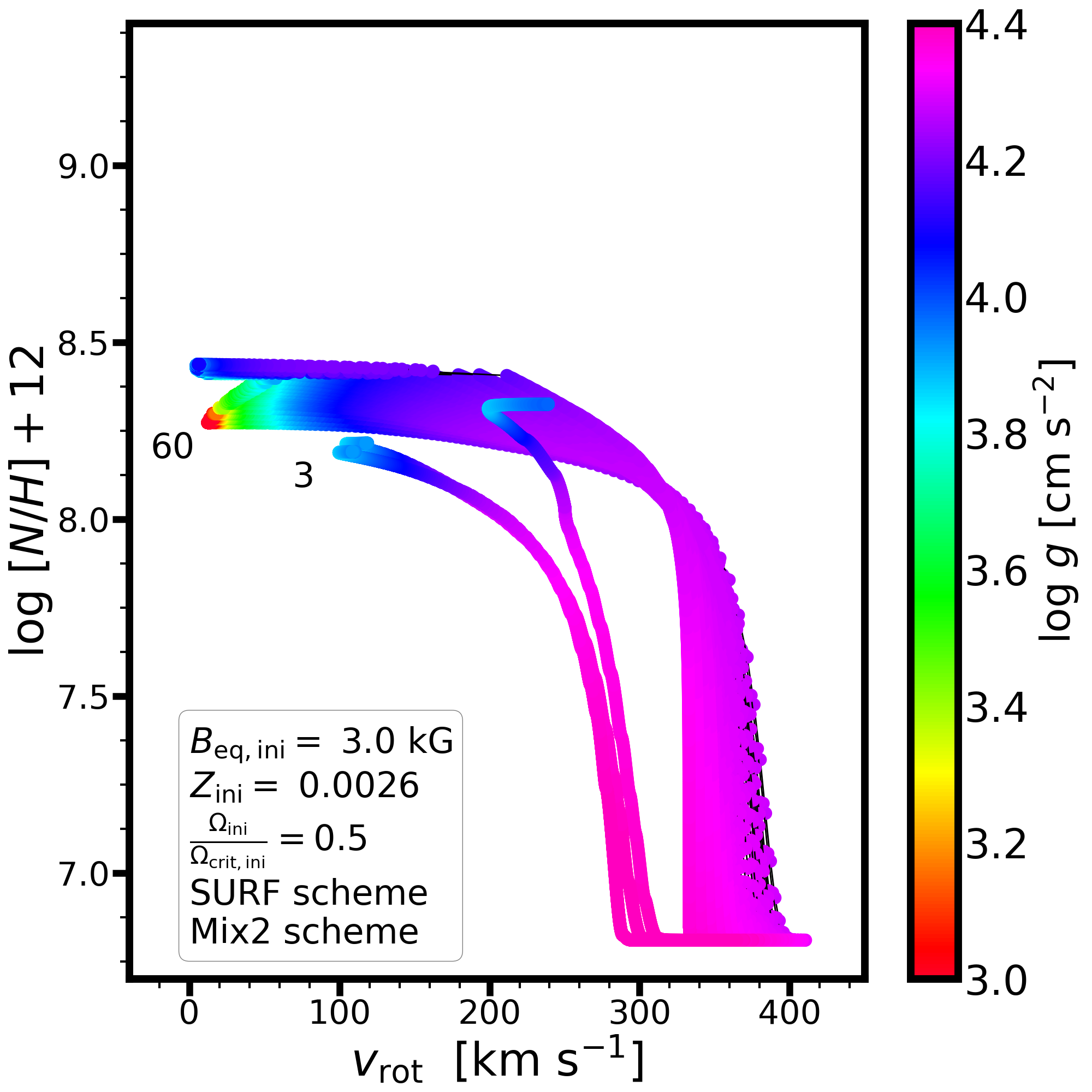
Figure 29: Same as Figure 28 but for the SURF/Mix2 scheme. See top panels of Figure 28 for the NOMAG/Mix2 models.

E.4 Impact of varying magnetic field strength at $Z=0.0026$

E.4.1 INT/Mix1

At SMC metallicity, the ZAMS position of the non-magnetic models is further shifted to higher effective temperatures compared to solar and LMC metallicity models (Figure 26). For the 50 and 60 M_⊙ models, we note major differences in comparison to models at higher metallicity. The highest mass non-magnetic models at SMC metallicity are able to undergo a blueward evolutionary phase for some fraction of their main sequence. This results from the relatively rapid rotation of the models, the efficient core-envelope coupling (assumed via hydrodynamic processes in a diffusive scheme), and the effects of stellar winds. These models can enhance their surface $[N/H]$ ratio by about a factor of 50 compared to the initial baseline value.

When a 0.5 kG initial equatorial magnetic field strength is considered, the effects of the spin-down are more pronounced than in higher metallicity models. We see that the blueward evolution of the most massive models is prevented. The impact on the nitrogen abundances is also notable as less enrichment is predicted compared to non-magnetic models. However, we should also note that in contrast to the most massive models in the INT/Mix1 scheme at higher metallicities, the rotational velocities of these models at SMC metallicity is actually less impacted. This is because stellar winds are less efficient at lower metallicity. Thus the combination of magnetic braking by a "weak" field (initially 0.5 kG) and weaker stellar winds allows for maintaining higher surface rotational velocities.

E.4.2 SURF/Mix1

In the SURF magnetic braking scheme we notice small differences compared to the INT scheme when keeping chemical mixing the same in the Mix1 scheme (Figure 27). For the same initial mass the SURF models tend to maintain a somewhat higher rotational velocity than the INT models. As expected, when increasing the value of the initial equatorial magnetic field strength from 0.5 to 3 kG, the spin-down is stronger, and consequently lower surface rotational velocities can be reached in conjunction with a reduction in the surface nitrogen enrichment. Nonetheless, the most massive models in this configuration with a 3 kG initial equatorial magnetic field strength are able to produce slowly-spinning, nitrogen-enriched Group 2 stars.

E.4.3 INT/Mix2

In the NOMAG/Mix2 at SMC metallicity, the most extended blueward evolution is produced, reaching 80 kK for the most massive stellar models (Figure 28). The behaviour of these models is qualitatively similar to those of solar and LMC metallicity. The predicted increase in $[N/H]$ is first a factor of about 50 related to mixing nitrogen, and then further almost a factor of 10 related to losing hydrogen from the stellar surface. Due to the blueward evolution of the models the surface gravities are expected to remain high.

In the INT/Mix2 case, a 0.5 and 3 kG initial equatorial magnetic field strength can prevent the extensive blueward evolution of the models. However, in contrast to some previous cases, the most massive models do not reach low surface gravities. Although for the non-magnetic case, all models are predicted to show a very large increase in their surface nitrogen abundance, the magnetic models show a more moderate enrichment. In this particular setup we also see that models less massive than initially 6 M_⊙ tend to produce much lower $[N/H]$ ratios, whereas models with higher initial masses are closely grouped together.

E.4.4 SURF/Mix2

In the SURF/Mix2 scheme at SMC metallicity the 0.5 kG initial magnetic field strength is not quite strong enough to prevent the quasi-chemically homogeneous evolution of the models (Figure 29). On the other hand, a 3 kG initial equatorial magnetic field strength leads to a more pronounced redward evolution of the most massive models after their spin-down. In this case, we again observe that the most massive models can reach low surface gravities along with low surface rotational velocities. In all cases, the predicted enrichment in $[N/H]$ remains over an order of magnitude compared to the baseline.

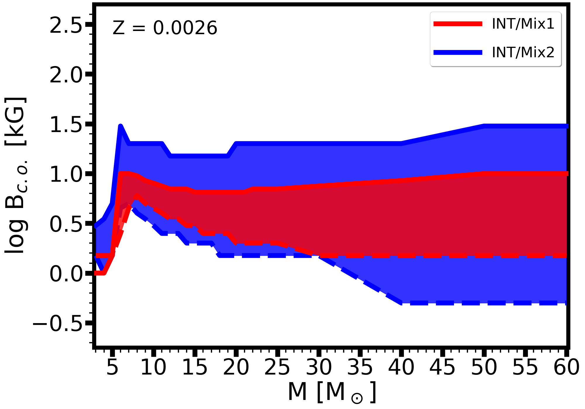
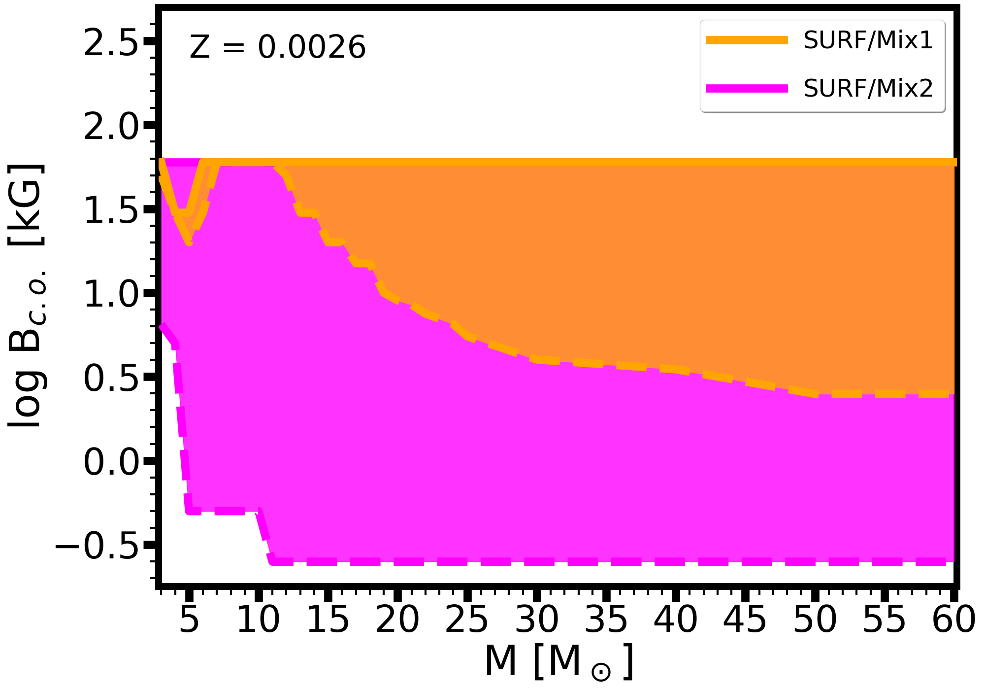
Figure 30: Cutoff magnetic field strengths in the Small Magellanic Cloud to produce slowly-rotating nitrogen enriched stars as a function of mass. Left/right panels show the INT/SURF schemes. The models are considered for an initial rotation of $\Omega/\Omega_{\rm crit}=0.5$ at SMC ($Z=0.0026$) metallicity.

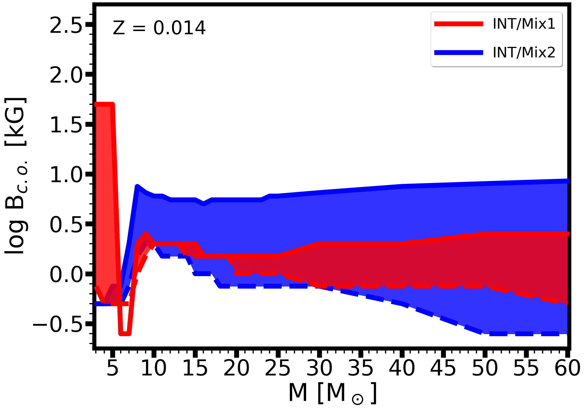
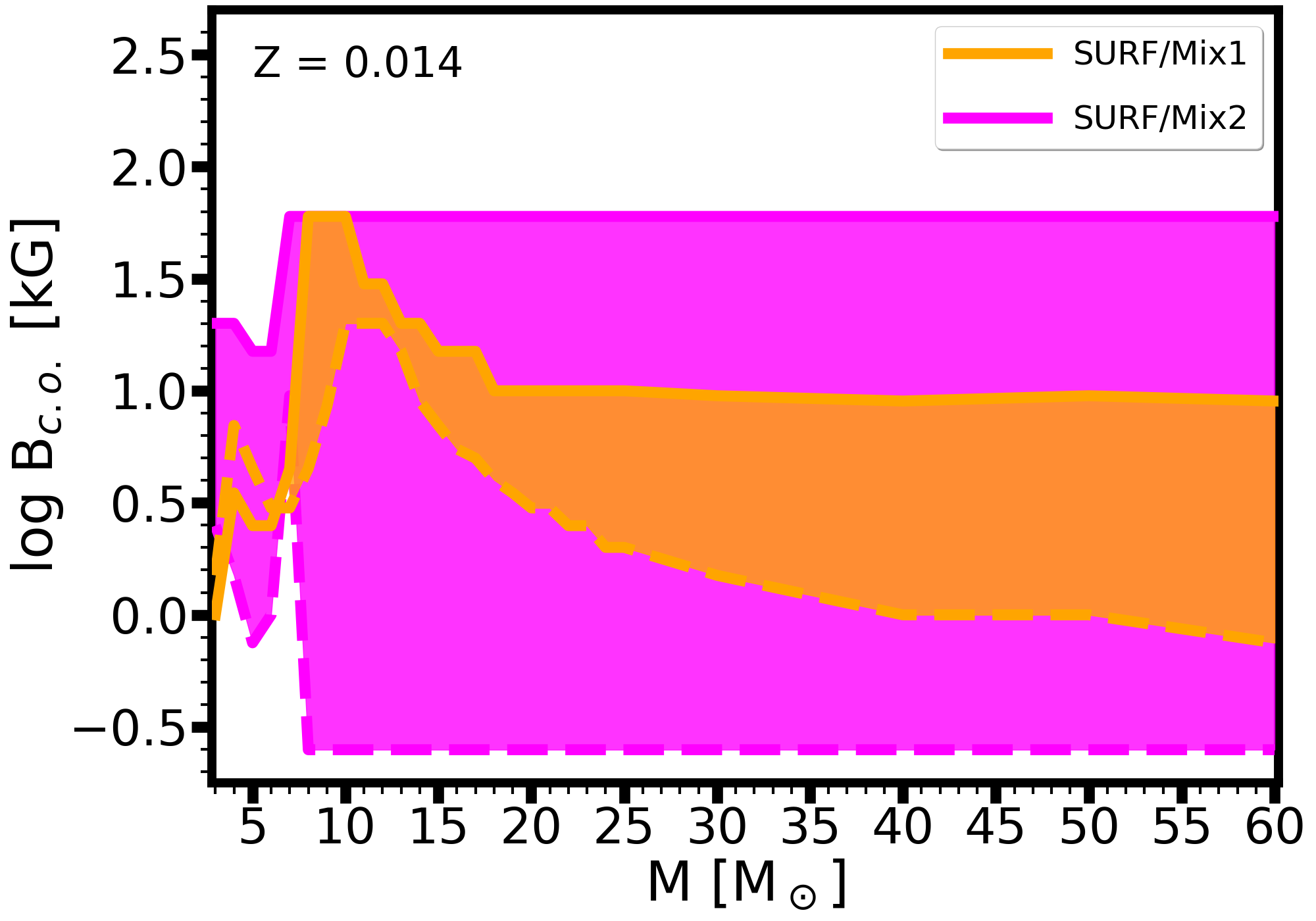
Figure 31: Same as Figure 30 but for Solar metallicity models.

Appendix F Cutoff magnetic field strength in the SMC and Solar neighbourhood

As in Section 4.2, we can quantify the cutoff magnetic field strengths in other metallicity environments needed to achieve slow-rotating, nitrogen-enriched stars. First, let us turn our attention to models at the SMC, shown in Figure 30. The four schemes predict essentially constant values for $B_{\rm max,N}$ for masses higher than about 10 M_⊙. The INT/Mix1 scheme is the most limiting scenario from the four schemes. The other schemes predict a wider range of magnetic field strengths that allow for producing Group 2 stars. Since nitrogen abundances and rotation rates are measurable in the SMC, the identified Group 2 stars (Dufton et al., 2020) could be explained with a limited range of magnetic field strengths. Typically, the magnetic field strength decreases roughly by an order of magnitude on the main sequence (cf. Equation 2). Thus depending on the age and evolutionary state of observed Group 2 stars, their observable fields will be weaker than the ZAMS field strengths. A sort of minimum range of their putative magnetic field strength could evolve from the range of initially 250 G to 7.5 kG (equatorial strength) at the ZAMS to 25 G to 750 G at the TAMS if the INT/Mix1 scheme is considered. For massive star models, the SURF/Mix1 and SURF/Mix2 schemes allow for an upper limit of initially 50 kG, which we expect to weaken to a 5 kG equatorial field strength by the TAMS.

Figure 31 shows models with an initial metallicity of $Z=~{}0.014$ (representative of the Solar neighbourhood). Consistently with previous findings, the INT/Mix1 is the most restrictive to produce Group 2 stars. In fact, in this case there are more forbidden regions than in models with lower metallicities. For example, the INT/Mix1 scheme essentially does not allow for producing Group 2 stars in the 6 - 23 M_⊙ range. In contrast, the SURF/Mix2 scheme allows for strong magnetic fields to brake the rotation and still produce nitrogen excess at the surface. Since high-resolution spectropolarimetric observations in the Galaxy have allowed for measuring the magnetic field strengths of massive stars, these model predictions allow for more direct comparison with observations than in the Magellanic Clouds. While the nitrogen abundance and (projected) rotational velocity are also measurable, a comprehensive study still needs to assess these three quantities jointly in comparison to magnetic stellar evolution models (however, see Morel et al. 2008; Martins et al. 2012; Martins et al. 2015; Aerts et al. 2014). Our single-star models provide testable predictions for these parameters, and such an investigation could help disentangle between the uncertain braking and mixing schemes. In particular, nitrogen-enriched slow rotators with strong magnetic fields favour efficient mixing.

References

- Aerts et al. (2003) Aerts C., Thoul A., Daszyńska J., Scuflaire R., Waelkens C., Dupret M. A., Niemczura E., Noels A., 2003, Science, 300, 1926
- Aerts et al. (2009) Aerts C., Puls J., Godart M., Dupret M. A., 2009, A&A, 508, 409
- Aerts et al. (2014) Aerts C., Molenberghs G., Kenward M. G., Neiner C., 2014, ApJ, 781, 88
- Aerts et al. (2019) Aerts C., Mathis S., Rogers T. M., 2019, ARA&A, 57, 35
- Aguilera-Dena et al. (2020) Aguilera-Dena D. R., Langer N., Antoniadis J., Müller B., 2020, ApJ, 901, 114
- Akgün et al. (2013) Akgün T., Reisenegger A., Mastrano A., Marchant P., 2013, MNRAS, 433, 2445
- Alecian et al. (2009) Alecian E., Wade G. A., Catala C., 2009, in Strassmeier K. G., Kosovichev A. G., Beckman J. E., eds, Vol. 259, Cosmic Magnetic Fields: From Planets, to Stars and Galaxies. pp 445–446 (arXiv:0812.3805), doi:10.1017/S1743921309031081
- Alecian et al. (2013) Alecian E., Wade G. A., Catala C., Grunhut J. H., Landstreet J. D., Böhm T., Folsom C. P., Marsden S., 2013, MNRAS, 429, 1027
- Alecian et al. (2016) Alecian E., Tkachenko A., Neiner C., Folsom C. P., Leroy B., 2016, A&A, 589, A47
- Alfvén (1942) Alfvén H., 1942, Nature, 150, 405
- Aloy & Obergaulinger (2021) Aloy M. Á., Obergaulinger M., 2021, MNRAS, 500, 4365
- Angulo et al. (1999) Angulo C., et al., 1999, Nuclear Phys. A, 656, 3
- Asplund et al. (2005) Asplund M., Grevesse N., Sauval A. J., 2005, in Barnes III T. G., Bash F. N., eds, Astronomical Society of the Pacific Conference Series Vol. 336, Cosmic Abundances as Records of Stellar Evolution and Nucleosynthesis. p. 25
- Asplund et al. (2009) Asplund M., Grevesse N., Sauval A. J., Scott P., 2009, ARA&A, 47, 481
- Augustson et al. (2016) Augustson K. C., Brun A. S., Toomre J., 2016, ApJ, 829, 92
- Aurière et al. (2007) Aurière M., et al., 2007, A&A, 475, 1053
- Babel & Montmerle (1997) Babel J., Montmerle T., 1997, A&A, 323, 121
- Bagnulo et al. (2017) Bagnulo S., et al., 2017, A&A, 601, A136
- Bagnulo et al. (2020) Bagnulo S., et al., 2020, A&A, 635, A163
- Barker et al. (2019) Barker A. J., Jones C. A., Tobias S. M., 2019, MNRAS, 487, 1777
- Barker et al. (2020) Barker A. J., Jones C. A., Tobias S. M., 2020, MNRAS, 495, 1468
- Bastian et al. (2020) Bastian N., Kamann S., Amard L., Charbonnel C., Haemmerlé L., Matt S. P., 2020, MNRAS, 495, 1978
- Beloborodov (2009) Beloborodov A. M., 2009, ApJ, 703, 1044
- Björklund et al. (2021) Björklund R., Sundqvist J. O., Puls J., Najarro F., 2021, A&A, 648, A36
- Bochenek et al. (2020) Bochenek C. D., Ravi V., Belov K. V., Hallinan G., Kocz J., Kulkarni S. R., McKenna D. L., 2020, Nature, 587, 59
- Bonaca et al. (2012) Bonaca A., et al., 2012, ApJ, 755, L12
- Bouret et al. (2005) Bouret J. C., Lanz T., Hillier D. J., 2005, A&A, 438, 301
- Bouret et al. (2021) Bouret J. C., Martins F., Hillier D. J., Marcolino W. L. F., Rocha-Pinto H. J., Georgy C., Lanz T., Hubeny I., 2021, A&A, 647, A134
- Bowman et al. (2020) Bowman D. M., Burssens S., Simón-Díaz S., Edelmann P. V. F., Rogers T. M., Horst L., Röpke F. K., Aerts C., 2020, A&A, 640, A36
- Braithwaite (2008) Braithwaite J., 2008, MNRAS, 386, 1947
- Braithwaite (2012) Braithwaite J., 2012, MNRAS, 422, 619
- Braithwaite & Nordlund (2006) Braithwaite J., Nordlund Å., 2006, A&A, 450, 1077
- Braithwaite & Spruit (2004) Braithwaite J., Spruit H. C., 2004, Nature, 431, 819
- Braithwaite & Spruit (2017) Braithwaite J., Spruit H. C., 2017, Royal Society Open Science, 4, 160271
- Brands et al. (2022) Brands S. A., et al., 2022, arXiv e-prints, p. arXiv:2202.11080
- Brinkman et al. (2021) Brinkman H. E., den Hartogh J. W., Doherty C. L., Pignatari M., Lugaro M., 2021, arXiv e-prints, p. arXiv:2109.05842
- Briquet et al. (2012) Briquet M., et al., 2012, MNRAS, 427, 483
- Brott et al. (2011a) Brott I., et al., 2011a, A&A, 530, A115
- Brott et al. (2011b) Brott I., et al., 2011b, A&A, 530, A116
- Burssens et al. (2020) Burssens S., et al., 2020, A&A, 639, A81
- Busse (1981) Busse F. H., 1981, Geophysical and Astrophysical Fluid Dynamics, 17, 215
- Busse (1982) Busse F. H., 1982, ApJ, 259, 759
- Buysschaert et al. (2018) Buysschaert B., Aerts C., Bowman D. M., Johnston C., Van Reeth T., Pedersen M. G., Mathis S., Neiner C., 2018, A&A, 616, A148
- CHIME/FRB Collaboration et al. (2020) CHIME/FRB Collaboration et al., 2020, Nature, 587, 54
- Caiazzo et al. (2021) Caiazzo I., et al., 2021, Nature, 595, 39
- Caleo et al. (2016) Caleo A., Balbus S. A., Tognelli E., 2016, MNRAS, 460, 338
- Cantiello & Braithwaite (2011) Cantiello M., Braithwaite J., 2011, A&A, 534, A140
- Cantiello et al. (2009) Cantiello M., et al., 2009, A&A, 499, 279
- Canuto & Mazzitelli (1992) Canuto V. M., Mazzitelli I., 1992, ApJ, 389, 724
- Canuto et al. (1996) Canuto V. M., Goldman I., Mazzitelli I., 1996, ApJ, 473, 550
- Cassisi et al. (2007) Cassisi S., Potekhin A. Y., Pietrinferni A., Catelan M., Salaris M., 2007, ApJ, 661, 1094
- Castor et al. (1975) Castor J. I., Abbott D. C., Klein R. I., 1975, ApJ, 195, 157
- Castro et al. (2014) Castro N., Fossati L., Langer N., Simón-Díaz S., Schneider F. R. N., Izzard R. G., 2014, A&A, 570, L13
- Cerrahoğlu et al. (2020) Cerrahoğlu P., Petit V., Keszthelyi Z., David-Uraz A., 2020, in Wade G., Alecian E., Bohlender D., Sigut A., eds, Vol. 11, Stellar Magnetism: A Workshop in Honour of the Career and Contributions of John D. Landstreet. pp 178–182 (arXiv:2001.10564)
- Chaboyer & Zahn (1992) Chaboyer B., Zahn J.-P., 1992, A&A, 253, 173
- Chang & Garaud (2021) Chang E., Garaud P., 2021, MNRAS, 506, 4914
- Charbonneau & MacGregor (2001) Charbonneau P., MacGregor K. B., 2001, ApJ, 559, 1094
- Charbonnel & Zahn (2007) Charbonnel C., Zahn J. P., 2007, A&A, 476, L29
- Chieffi & Limongi (2013) Chieffi A., Limongi M., 2013, ApJ, 764, 21
- Choi et al. (2016) Choi J., Dotter A., Conroy C., Cantiello M., Paxton B., Johnson B. D., 2016, ApJ, 823, 102
- Chugunov et al. (2007) Chugunov A. I., Dewitt H. E., Yakovlev D. G., 2007, Phys. Rev. D, 76, 025028
- Cohen et al. (2003) Cohen D. H., de Messières G. E., MacFarlane J. J., Miller N. A., Cassinelli J. P., Owocki S. P., Liedahl D. A., 2003, ApJ, 586, 495
- Commerçon et al. (2011) Commerçon B., Hennebelle P., Henning T., 2011, ApJ, 742, L9
- Costa et al. (2019) Costa G., Girardi L., Bressan A., Marigo P., Rodrigues T. S., Chen Y., Lanza A., Goudfrooij P., 2019, MNRAS, 485, 4641
- Costa et al. (2021) Costa G., Bressan A., Mapelli M., Marigo P., Iorio G., Spera M., 2021, MNRAS, 501, 4514
- Cowling (1945) Cowling T. G., 1945, MNRAS, 105, 166
- Crowther et al. (2006) Crowther P. A., Lennon D. J., Walborn N. R., 2006, A&A, 446, 279
- Crutcher (2012) Crutcher R. M., 2012, Annual Review of Astronomy and Astrophysics, 50, 29
- Cyburt et al. (2010) Cyburt R. H., et al., 2010, ApJS, 189, 240
- D’Antona et al. (2015) D’Antona F., Di Criscienzo M., Decressin T., Milone A. P., Vesperini E., Ventura P., 2015, MNRAS, 453, 2637
- Das et al. (2020) Das B., Chandra P., Wade G. A., 2020, MNRAS, 499, 702
- David-Uraz et al. (2019) David-Uraz A., et al., 2019, MNRAS, 487, 304
- David-Uraz et al. (2021a) David-Uraz A., Petit V., Shultz M. E., Fullerton A. W., Erba C., Keszthelyi Z., Seadrow S., Wade G. A., 2021a, MNRAS, 501, 2677
- David-Uraz et al. (2021b) David-Uraz A., et al., 2021b, MNRAS, 504, 4841
- Deal et al. (2021) Deal M., Cunha M. S., Keszthelyi Z., Perraut K., Holdsworth D. L., 2021, A&A, 650, A125
- Denissenkov & Pinsonneault (2007) Denissenkov P. A., Pinsonneault M., 2007, ApJ, 655, 1157
- Denissenkov et al. (2009) Denissenkov P. A., Pinsonneault M., MacGregor K. B., 2009, ApJ, 696, 1823
- Donati & Landstreet (2009) Donati J.-F., Landstreet J. D., 2009, ARA&A, 47, 333
- Donati et al. (2002) Donati J. F., Babel J., Harries T. J., Howarth I. D., Petit P., Semel M., 2002, Monthly Notices of the Royal Astronomical Society, 333, 55
- Donati et al. (2006) Donati J. F., et al., 2006, MNRAS, 370, 629
- Dopita et al. (2019) Dopita M. A., Seitenzahl I. R., Sutherland R. S., Nicholls D. C., Vogt F. P. A., Ghavamian P., Ruiter A. J., 2019, AJ, 157, 50
- Driessen et al. (2019a) Driessen F. A., Sundqvist J. O., Wade G. A., 2019a, IAU Symposium, 346, 45
- Driessen et al. (2019b) Driessen F. A., Sundqvist J. O., Kee N. D., 2019b, A&A, 631, A172
- Duez & Mathis (2010) Duez V., Mathis S., 2010, A&A, 517, A58
- Duez et al. (2010) Duez V., Mathis S., Turck-Chièze S., 2010, MNRAS, 402, 271
- Dufton et al. (2006) Dufton P. L., Ryans R. S. I., Simón-Díaz S., Trundle C., Lennon D. J., 2006, A&A, 451, 603
- Dufton et al. (2013) Dufton P. L., et al., 2013, A&A, 550, A109
- Dufton et al. (2018) Dufton P. L., et al., 2018, A&A, 615, A101
- Dufton et al. (2019) Dufton P. L., Evans C. J., Hunter I., Lennon D. J., Schneider F. R. N., 2019, A&A, 626, A50
- Dufton et al. (2020) Dufton P. L., Evans C. J., Lennon D. J., Hunter I., 2020, A&A, 634, A6
- Eddington (1925) Eddington A. S., 1925, The Observatory, 48, 73
- Eggenberger et al. (2008) Eggenberger P., Meynet G., Maeder A., Hirschi R., Charbonnel C., Talon S., Ekström S., 2008, Ap&SS, 316, 43
- Ekström et al. (2012) Ekström S., et al., 2012, A&A, 537, A146
- Endal & Sofia (1978) Endal A. S., Sofia S., 1978, ApJ, 220, 279
- Erba et al. (2021) Erba C., et al., 2021, MNRAS, 506, 5373
- Espinosa Lara & Rieutord (2011) Espinosa Lara F., Rieutord M., 2011, A&A, 533, A43
- Featherstone et al. (2009) Featherstone N. A., Browning M. K., Brun A. S., Toomre J., 2009, ApJ, 705, 1000
- Feiden (2016) Feiden G. A., 2016, A&A, 593, A99
- Feiden & Chaboyer (2012) Feiden G. A., Chaboyer B., 2012, ApJ, 761, 30
- Feiden & Chaboyer (2013) Feiden G. A., Chaboyer B., 2013, ApJ, 779, 183
- Feiden & Chaboyer (2014) Feiden G. A., Chaboyer B., 2014, ApJ, 789, 53
- Ferguson et al. (2005) Ferguson J. W., Alexander D. R., Allard F., Barman T., Bodnarik J. G., Hauschildt P. H., Heffner-Wong A., Tamanai A., 2005, ApJ, 623, 585
- Ferrario et al. (2009) Ferrario L., Pringle J. E., Tout C. A., Wickramasinghe D. T., 2009, MNRAS, 400, L71
- Ferrario et al. (2015) Ferrario L., Melatos A., Zrake J., 2015, Space Sci. Rev., 191, 77
- Ferrario et al. (2020) Ferrario L., Wickramasinghe D., Kawka A., 2020, Advances in Space Research, 66, 1025
- Ferraro (1937) Ferraro V. C. A., 1937, MNRAS, 97, 458
- Fossati et al. (2016) Fossati L., et al., 2016, A&A, 592, A84
- Fricke (1968) Fricke K., 1968, Z. Astrophys., 68, 317
- Fuller & Ma (2019) Fuller J., Ma L., 2019, ApJ, 881, L1
- Fuller et al. (1985) Fuller G. M., Fowler W. A., Newman M. J., 1985, ApJ, 293, 1
- Fuller et al. (2015) Fuller J., Cantiello M., Stello D., Garcia R. A., Bildsten L., 2015, Science, 350, 423
- Fuller et al. (2019) Fuller J., Piro A. L., Jermyn A. S., 2019, MNRAS, 485, 3661
- Fullerton et al. (2006) Fullerton A. W., Massa D. L., Prinja R. K., 2006, ApJ, 637, 1025
- Gagnier et al. (2019a) Gagnier D., Rieutord M., Charbonnel C., Putigny B., Espinosa Lara F., 2019a, A&A, 625, A88
- Gagnier et al. (2019b) Gagnier D., Rieutord M., Charbonnel C., Putigny B., Espinosa Lara F., 2019b, A&A, 625, A89
- Georgy et al. (2012) Georgy C., Ekström S., Meynet G., Massey P., Levesque E. M., Hirschi R., Eggenberger P., Maeder A., 2012, A&A, 542, A29
- Georgy et al. (2013) Georgy C., et al., 2013, A&A, 558, A103
- Georgy et al. (2017) Georgy C., Meynet G., Ekström S., Wade G. A., Petit V., Keszthelyi Z., Hirschi R., 2017, A&A, 599, L5
- Giacomazzo et al. (2015) Giacomazzo B., Zrake J., Duffell P. C., MacFadyen A. I., Perna R., 2015, ApJ, 809, 39
- Goldreich & Schubert (1967) Goldreich P., Schubert G., 1967, ApJ, 150, 571
- Goldstein et al. (2019) Goldstein J., Townsend R. H. D., Zweibel E. G., 2019, ApJ, 881, 66
- Gough & Tayler (1966) Gough D. O., Tayler R. J., 1966, MNRAS, 133, 85
- Gräfener et al. (2012) Gräfener G., Owocki S. P., Vink J. S., 2012, A&A, 538, A40
- Grasha et al. (2021) Grasha K., Roy A., Sutherland R. S., Kewley L. J., 2021, ApJ, 908, 241
- Gregory (2011) Gregory S. G., 2011, American Journal of Physics, 79, 461
- Grin et al. (2017) Grin N. J., et al., 2017, A&A, 600, A82
- Groh et al. (2019) Groh J. H., et al., 2019, A&A, 627, A24
- Grunhut et al. (2012) Grunhut J. H., et al., 2012, MNRAS, 419, 1610
- Grunhut et al. (2017) Grunhut J. H., et al., 2017, MNRAS, 465, 2432
- Harrington & Garaud (2019) Harrington P. Z., Garaud P., 2019, ApJ, 870, L5
- Heger et al. (2000) Heger A., Langer N., Woosley S. E., 2000, ApJ, 528, 368
- Heger et al. (2005) Heger A., Woosley S. E., Spruit H. C., 2005, ApJ, 626, 350
- Hennebelle (2013) Hennebelle P., 2013, A&A, 556, A153
- Henrichs et al. (2013) Henrichs H. F., et al., 2013, A&A, 555, A46
- Henyey et al. (1965) Henyey L., Vardya M. S., Bodenheimer P., 1965, ApJ, 142, 841
- Høiland (1941) Høiland K., 1941, Avhandliger Norske Videnskaps-Akademi i Oslo, I,math.-naturv. Klasse, 11, 1
- Holgado et al. (2022) Holgado G., Simón-Díaz S., Herrero A., Barbá R. H., 2022, arXiv e-prints, p. arXiv:2207.12776
- Howarth et al. (1997) Howarth I. D., Siebert K. W., Hussain G. A. J., Prinja R. K., 1997, MNRAS, 284, 265
- Huang et al. (2010) Huang W., Gies D. R., McSwain M. V., 2010, ApJ, 722, 605
- Hunter et al. (2008) Hunter I., et al., 2008, ApJ, 676, L29
- Hunter et al. (2009) Hunter I., et al., 2009, A&A, 496, 841
- Iglesias & Rogers (1993) Iglesias C. A., Rogers F. J., 1993, ApJ, 412, 752
- Iglesias & Rogers (1996) Iglesias C. A., Rogers F. J., 1996, ApJ, 464, 943
- Irwin (2004) Irwin A. W., 2004, The FreeEOS Code for Calculating the Equation of State for Stellar Interiors, http://freeeos.sourceforge.net/
- Itoh et al. (1996) Itoh N., Hayashi H., Nishikawa A., Kohyama Y., 1996, ApJS, 102, 411
- Jardine et al. (1999) Jardine M., Barnes J. R., Donati J.-F., Collier Cameron A., 1999, MNRAS, 305, L35
- Jermyn & Cantiello (2020) Jermyn A. S., Cantiello M., 2020, ApJ, 900, 113
- Jermyn et al. (2021) Jermyn A. S., Schwab J., Bauer E., Timmes F. X., Potekhin A. Y., 2021, ApJ, 913, 72
- Keszthelyi et al. (2017a) Keszthelyi Z., Wade G. A., Petit V., 2017a, in Eldridge J. J., Bray J. C., McClelland L. A. S., Xiao L., eds, IAU Symposium Vol. 329, The Lives and Death-Throes of Massive Stars. pp 250–254 (arXiv:1702.04460), doi:10.1017/S1743921317002745
- Keszthelyi et al. (2017b) Keszthelyi Z., Puls J., Wade G. A., 2017b, A&A, 598, A4
- Keszthelyi et al. (2019) Keszthelyi Z., Meynet G., Georgy C., Wade G. A., Petit V., David-Uraz A., 2019, MNRAS, 485, 5843
- Keszthelyi et al. (2020) Keszthelyi Z., et al., 2020, MNRAS, 493, 518
- Keszthelyi et al. (2021) Keszthelyi Z., Meynet G., Martins F., de Koter A., David-Uraz A., 2021, MNRAS, 504, 2474
- Khalack et al. (2003) Khalack V. R., Zverko J., Žižňovský J., 2003, A&A, 403, 179
- Kippenhahn (1974) Kippenhahn R., 1974, in Tayler R. J., Hesser J. E., eds, IAU Symposium, No. 66 Vol. 66, Late Stages of Stellar Evolution. p. 20
- Kissin & Thompson (2018) Kissin Y., Thompson C., 2018, ApJ, 862, 111
- Knigge et al. (2009) Knigge C., Leigh N., Sills A., 2009, Nature, 457, 288
- Kochukhov & Bagnulo (2006) Kochukhov O., Bagnulo S., 2006, A&A, 450, 763
- Kochukhov & Wade (2016) Kochukhov O., Wade G. A., 2016, A&A, 586, A30
- Kochukhov et al. (2019) Kochukhov O., Shultz M., Neiner C., 2019, A&A, 621, A47
- Körtgen & Soler (2020) Körtgen B., Soler J. D., 2020, Monthly Notices of the Royal Astronomical Society, 499, 4785
- Krtička (2014) Krtička J., 2014, A&A, 564, A70
- Krtička & Kubát (2017) Krtička J., Kubát J., 2017, A&A, 606, A31
- Krtička et al. (2021) Krtička J., Kubát J., Krtičková I., 2021, A&A, 647, A28
- Kudritzki & Puls (2000) Kudritzki R.-P., Puls J., 2000, ARA&A, 38, 613
- Kulsrud (2005) Kulsrud R. M., 2005, Plasma physics for astrophysics. Princeton University Press
- Kuroda et al. (2020) Kuroda T., Arcones A., Takiwaki T., Kotake K., 2020, ApJ, 896, 102
- Lamers et al. (1995) Lamers H. J. G. L. M., Snow T. P., Lindholm D. M., 1995, ApJ, 455, 269
- Landstreet (1991) Landstreet J. D., 1991, The Boundary Between the Magnetic Fields of Ap-Stars and the Fields of Solar-Type Stars. p. 342, doi:10.1007/3-540-53955-7_153
- Landstreet & Borra (1978) Landstreet J. D., Borra E. F., 1978, ApJ, 224, L5
- Landstreet et al. (2007) Landstreet J. D., Bagnulo S., Andretta V., Fossati L., Mason E., Silaj J., Wade G. A., 2007, A&A, 470, 685
- Landstreet et al. (2008) Landstreet J. D., et al., 2008, A&A, 481, 465
- Langanke & Martínez-Pinedo (2000) Langanke K., Martínez-Pinedo G., 2000, Nuclear Physics A, 673, 481
- Laplace (2021) Laplace E., 2021, arXiv e-prints, p. arXiv:2111.05346
- Lavail et al. (2020) Lavail A., Kochukhov O., Hussain G. A. J., Argiroffi C., Alecian E., Morin J., BinaMIcS Collaboration 2020, MNRAS, 497, 632
- Lecoanet et al. (2022) Lecoanet D., Bowman D. M., Van Reeth T., 2022, arXiv e-prints, p. arXiv:2202.03440
- Lennon et al. (1996) Lennon D. J., Dufton P. L., Mazzali P. A., Pasian F., Marconi G., 1996, A&A, 314, 243
- Lennon et al. (2003) Lennon D. J., Dufton P. L., Crowley C., 2003, A&A, 398, 455
- Leto et al. (2018) Leto P., et al., 2018, MNRAS, 476, 562
- Leto et al. (2021) Leto P., et al., 2021, MNRAS, 507, 1979
- Lodders (2003) Lodders K., 2003, ApJ, 591, 1220
- Lovekin (2020) Lovekin C. C., 2020, Frontiers in Astronomy and Space Sciences, 6, 77
- Lucy & Solomon (1970) Lucy L. B., Solomon P. M., 1970, ApJ, 159, 879
- Lydon & Sofia (1995) Lydon T. J., Sofia S., 1995, ApJS, 101, 357
- MacDonald & Mullan (2017) MacDonald J., Mullan D. J., 2017, ApJ, 850, 58
- MacDonald & Petit (2019) MacDonald J., Petit V., 2019, MNRAS, 487, 3904
- Mackey & Lim (2011) Mackey J., Lim A. J., 2011, MNRAS, 412, 2079
- Maeder (1987) Maeder A., 1987, A&A, 178, 159
- Maeder (1997) Maeder A., 1997, A&A, 321, 134
- Maeder (2009) Maeder A., 2009, Physics, Formation and Evolution of Rotating Stars, doi:10.1007/978-3-540-76949-1.
- Maeder & Meynet (2000) Maeder A., Meynet G., 2000, A&A, 361, 159
- Maeder & Meynet (2003) Maeder A., Meynet G., 2003, A&A, 411, 543
- Maeder & Meynet (2004) Maeder A., Meynet G., 2004, A&A, 422, 225
- Maeder & Meynet (2005) Maeder A., Meynet G., 2005, A&A, 440, 1041
- Maeder & Zahn (1998) Maeder A., Zahn J.-P., 1998, A&A, 334, 1000
- Maeder et al. (2013) Maeder A., Meynet G., Lagarde N., Charbonnel C., 2013, A&A, 553, A1
- Maeder et al. (2014) Maeder A., Przybilla N., Nieva M.-F., Georgy C., Meynet G., Ekström S., Eggenberger P., 2014, A&A, 565, A39
- Makarenko et al. (2021) Makarenko E. I., Igoshev A. P., Kholtygin A. F., 2021, Monthly Notices of the Royal Astronomical Society, 504, 5813
- Marcolino et al. (2012) Marcolino W. L. F., et al., 2012, MNRAS, 422, 2314
- Markova & Puls (2008) Markova N., Puls J., 2008, A&A, 478, 823
- Markova et al. (2018) Markova N., Puls J., Langer N., 2018, A&A, 613, A12
- Martayan et al. (2006) Martayan C., Frémat Y., Hubert A. M., Floquet M., Zorec J., Neiner C., 2006, A&A, 452, 273
- Martayan et al. (2007) Martayan C., Frémat Y., Hubert A. M., Floquet M., Zorec J., Neiner C., 2007, A&A, 462, 683
- Martin et al. (2018) Martin A. J., et al., 2018, MNRAS, 475, 1521
- Martins et al. (2012) Martins F., Escolano C., Wade G. A., Donati J. F., Bouret J. C., Mimes Collaboration 2012, A&A, 538, A29
- Martins et al. (2013) Martins F., Depagne E., Russeil D., Mahy L., 2013, A&A, 554, A23
- Martins et al. (2015) Martins F., et al., 2015, A&A, 575, A34
- Martins et al. (2017) Martins F., Simón-Díaz S., Barbá R. H., Gamen R. C., Ekström S., 2017, A&A, 599, A30
- Masada et al. (2022) Masada Y., Takiwaki T., Kotake K., 2022, ApJ, 924, 75
- McEvoy et al. (2015) McEvoy C. M., et al., 2015, A&A, 575, A70
- Mestel (1967) Mestel L., 1967, in Cameron R. C., ed., Magnetic and Related Stars. p. 101
- Mestel (1968) Mestel L., 1968, MNRAS, 138, 359
- Mestel (1989) Mestel L., 1989, QJRAS, 30, 239
- Mestel (1999) Mestel L., 1999, Stellar magnetism
- Mestel (2003) Mestel L., 2003, in Balona L. A., Henrichs H. F., Medupe R., eds, Astronomical Society of the Pacific Conference Series Vol. 305, Magnetic Fields in O, B and A Stars: Origin and Connection to Pulsation, Rotation and Mass Loss. p. 3
- Mestel & Moss (2010) Mestel L., Moss D., 2010, MNRAS, 405, 1845
- Meynet et al. (2011) Meynet G., Eggenberger P., Maeder A., 2011, A&A, 525, L11
- Meynet et al. (2013) Meynet G., Ekstrom S., Maeder A., Eggenberger P., Saio H., Chomienne V., Haemmerlé L., 2013, in Goupil M., Belkacem K., Neiner C., Lignières F., Green J. J., eds, Lecture Notes in Physics, Berlin Springer Verlag Vol. 865, Lecture Notes in Physics, Berlin Springer Verlag. p. 3 (arXiv:1301.2487), doi:10.1007/978-3-642-33380-4_1
- Michielsen et al. (2021) Michielsen M., Aerts C., Bowman D. M., 2021, A&A, 650, A175
- Mokiem et al. (2007) Mokiem M. R., et al., 2007, A&A, 473, 603
- Morel et al. (2008) Morel T., Hubrig S., Briquet M., 2008, A&A, 481, 453
- Morel et al. (2015) Morel T., et al., 2015, in Meynet G., Georgy C., Groh J., Stee P., eds, IAU Symposium Vol. 307, New Windows on Massive Stars. pp 342–347 (arXiv:1408.2100), doi:10.1017/S1743921314007054
- Moss (2003) Moss D., 2003, A&A, 403, 693
- Mösta et al. (2015) Mösta P., Ott C. D., Radice D., Roberts L. F., Schnetter E., Haas R., 2015, Nature, 528, 376
- Moyano et al. (2022) Moyano F. D., Eggenberger P., Meynet G., Gehan C., Mosser B., Buldgen G., Salmon S. J. A. J., 2022, arXiv e-prints, p. arXiv:2205.03490
- Muijres et al. (2012) Muijres L. E., Vink J. S., de Koter A., Müller P. E., Langer N., 2012, A&A, 537, A37
- Mullan & MacDonald (2001) Mullan D. J., MacDonald J., 2001, ApJ, 559, 353
- Munoz et al. (2020) Munoz M. S., Wade G. A., Nazé Y., Puls J., Bagnulo S., Szymański M. K., 2020, MNRAS, 492, 1199
- Murphy et al. (2021) Murphy L. J., et al., 2021, MNRAS, 501, 2745
- Nazé et al. (2014) Nazé Y., Petit V., Rinbrand M., Cohen D., Owocki S., ud-Doula A., Wade G. A., 2014, ApJS, 215, 10
- Neiner et al. (2015) Neiner C., Mathis S., Alecian E., Emeriau C., Grunhut J., BinaMIcS MiMeS Collaborations 2015, in Nagendra K. N., Bagnulo S., Centeno R., Jesús Martínez González M., eds, IAU Symposium Vol. 305, Polarimetry. pp 61–66 (arXiv:1502.00226), doi:10.1017/S1743921315004524
- Neiner et al. (2017) Neiner C., et al., 2017, MNRAS, 471, 1926
- Neronov & Vovk (2010) Neronov A., Vovk I., 2010, Science, 328, 73
- Nieva & Przybilla (2012) Nieva M.-F., Przybilla N., 2012, A&A, 539, A143
- Nugis & Lamers (2002) Nugis T., Lamers H. J. G. L. M., 2002, A&A, 389, 162
- Oda et al. (1994) Oda T., Hino M., Muto K., Takahara M., Sato K., 1994, Atomic Data and Nuclear Data Tables, 56, 231
- Oksala et al. (2010) Oksala M. E., Wade G. A., Marcolino W. L. F., Grunhut J., Bohlender D., Manset N., Townsend R. H. D., Mimes Collaboration 2010, MNRAS, 405, L51
- Oksala et al. (2012) Oksala M. E., Wade G. A., Townsend R. H. D., Owocki S. P., Kochukhov O., Neiner C., Alecian E., Grunhut J., 2012, MNRAS, 419, 959
- Oksala et al. (2015) Oksala M. E., Grunhut J. H., Kraus M., Borges Fernandes M., Neiner C., Condori C. A. H., Campagnolo J. C. N., Souza T. B., 2015, A&A, 578, A112
- Owocki & ud-Doula (2004) Owocki S. P., ud-Doula A., 2004, ApJ, 600, 1004
- Owocki et al. (2016) Owocki S. P., ud-Doula A., Sundqvist J. O., Petit V., Cohen D. H., Townsend R. H. D., 2016, MNRAS, 462, 3830
- Owocki et al. (2020) Owocki S. P., Shultz M. E., ud-Doula A., Sundqvist J. O., Townsend R. H. D., Cranmer S. R., 2020, MNRAS, 499, 5366
- Park et al. (2021) Park J., Prat V., Mathis S., Bugnet L., 2021, A&A, 646, A64
- Parker (1958) Parker E. N., 1958, ApJ, 128, 664
- Parker (1963) Parker E. N., 1963, Interplanetary dynamical processes.
- Pauldrach et al. (1986) Pauldrach A., Puls J., Kudritzki R. P., 1986, A&A, 164, 86
- Paxton et al. (2011) Paxton B., Bildsten L., Dotter A., Herwig F., Lesaffre P., Timmes F., 2011, ApJS, 192, 3
- Paxton et al. (2013) Paxton B., et al., 2013, ApJS, 208, 4
- Paxton et al. (2015) Paxton B., et al., 2015, ApJS, 220, 15
- Paxton et al. (2018) Paxton B., et al., 2018, ApJS, 234, 34
- Paxton et al. (2019) Paxton B., et al., 2019, ApJS, 243, 10
- Pedersen et al. (2021) Pedersen M. G., et al., 2021, Nature Astronomy, 5, 715
- Petermann et al. (2015) Petermann I., Langer N., Castro N., Fossati L., 2015, A&A, 584, A54
- Petit et al. (2013) Petit V., et al., 2013, MNRAS, 429, 398
- Petit et al. (2017) Petit V., et al., 2017, MNRAS, 466, 1052
- Petit et al. (2019) Petit V., et al., 2019, MNRAS, 489, 5669
- Petrov et al. (2016) Petrov B., Vink J. S., Gräfener G., 2016, MNRAS, 458, 1999
- Pinsonneault et al. (1989) Pinsonneault M. H., Kawaler S. D., Sofia S., Demarque P., 1989, ApJ, 338, 424
- Poniatowski et al. (2021) Poniatowski L. G., et al., 2021, A&A, 647, A151
- Potekhin & Chabrier (2010) Potekhin A. Y., Chabrier G., 2010, Contributions to Plasma Physics, 50, 82
- Potter et al. (2012a) Potter A. T., Tout C. A., Eldridge J. J., 2012a, MNRAS, 419, 748
- Potter et al. (2012b) Potter A. T., Chitre S. M., Tout C. A., 2012b, MNRAS, 424, 2358
- Poutanen (2017) Poutanen J., 2017, ApJ, 835, 119
- Prat et al. (2016) Prat V., Guilet J., Viallet M., Müller E., 2016, A&A, 592, A59
- Prinja & Massa (1998) Prinja R. K., Massa D. L., 1998, in Howarth I., ed., Astronomical Society of the Pacific Conference Series Vol. 131, Properties of Hot Luminous Stars. p. 218
- Prinja et al. (1990) Prinja R. K., Barlow M. J., Howarth I. D., 1990, ApJ, 361, 607
- Przybilla et al. (2008) Przybilla N., Nieva M.-F., Butler K., 2008, ApJ, 688, L103
- Przybilla et al. (2013) Przybilla N., Nieva M. F., Irrgang A., Butler K., 2013, in Alecian G., Lebreton Y., Richard O., Vauclair G., eds, EAS Publications Series Vol. 63, EAS Publications Series. pp 13–23, doi:10.1051/eas/1363002
- Puls et al. (2000) Puls J., Springmann U., Lennon M., 2000, A&AS, 141, 23
- Puls et al. (2008) Puls J., Vink J. S., Najarro F., 2008, A&ARv, 16, 209
- Quentin & Tout (2018) Quentin L. G., Tout C. A., 2018, MNRAS, 477, 2298
- Ramachandran et al. (2021) Ramachandran V., Oskinova L. M., Hamann W. R., 2021, A&A, 646, A16
- Ramírez-Agudelo et al. (2013) Ramírez-Agudelo O. H., et al., 2013, A&A, 560, A29
- Ramírez-Agudelo et al. (2015) Ramírez-Agudelo O. H., et al., 2015, A&A, 580, A92
- Reboul-Salze et al. (2021) Reboul-Salze A., Guilet J., Raynaud R., Bugli M., 2021, A&A, 645, A109
- Reese et al. (2021) Reese D. R., Mirouh G. M., Espinosa Lara F., Rieutord M., Putigny B., 2021, A&A, 645, A46
- Reisenegger (2009) Reisenegger A., 2009, A&A, 499, 557
- Rieutord (2006) Rieutord M., 2006, in Rieutord M., Dubrulle B., eds, EAS Publications Series Vol. 21, EAS Publications Series. pp 275–295 (arXiv:astro-ph/0608431), doi:10.1051/eas:2006117
- Rivero González et al. (2012) Rivero González J. G., Puls J., Najarro F., Brott I., 2012, A&A, 537, A79
- Rivinius et al. (2013) Rivinius T., Townsend R. H. D., Kochukhov O., Štefl S., Baade D., Barrera L., Szeifert T., 2013, MNRAS, 429, 177
- Rogers & Nayfonov (2002) Rogers F. J., Nayfonov A., 2002, ApJ, 576, 1064
- Rubio-Díez et al. (2022) Rubio-Díez M. M., Sundqvist J. O., Najarro F., Traficante A., Puls J., Calzoletti L., Figer D., 2022, A&A, 658, A61
- Salaris & Cassisi (2017) Salaris M., Cassisi S., 2017, Royal Society Open Science, 4, 170192
- Sana et al. (2012) Sana H., et al., 2012, Science, 337, 444
- Sana et al. (2014) Sana H., et al., 2014, ApJS, 215, 15
- Saumon et al. (1995) Saumon D., Chabrier G., van Horn H. M., 1995, ApJS, 99, 713
- Schaller et al. (1992) Schaller G., Schaerer D., Meynet G., Maeder A., 1992, A&AS, 96, 269
- Schneider et al. (2016) Schneider F. R. N., Podsiadlowski P., Langer N., Castro N., Fossati L., 2016, MNRAS, 457, 2355
- Schneider et al. (2018) Schneider F. R. N., et al., 2018, A&A, 618, A73
- Schneider et al. (2019) Schneider F. R. N., Ohlmann S. T., Podsiadlowski P., Röpke F. K., Balbus S. A., Pakmor R., Springel V., 2019, Nature, 574, 211
- Schneider et al. (2020) Schneider F. R. N., Ohlmann S. T., Podsiadlowski P., Röpke F. K., Balbus S. A., Pakmor R., 2020, MNRAS, 495, 2796
- Schüssler & Knölker (2001) Schüssler M., Knölker M., 2001, in Mathys G., Solanki S. K., Wickramasinghe D. T., eds, Astronomical Society of the Pacific Conference Series Vol. 248, Magnetic Fields Across the Hertzsprung-Russell Diagram. p. 115
- Seifried et al. (2020) Seifried D., Walch S., Weis M., Reissl S., Soler J., Klessen R., Joshi P., 2020, Monthly Notices of the Royal Astronomical Society, 497, 4196
- Shultz et al. (2015) Shultz M., Wade G. A., Alecian E., BinaMIcS Collaboration 2015, MNRAS, 454, L1
- Shultz et al. (2018) Shultz M. E., et al., 2018, MNRAS, 475, 5144
- Shultz et al. (2019a) Shultz M. E., Wade G. A., Rivinius T., Alecian E., Neiner C., Petit V., Wisniewski J. P., 2019a, MNRAS, 485, 1508
- Shultz et al. (2019b) Shultz M. E., et al., 2019b, MNRAS, 490, 274
- Shultz et al. (2019c) Shultz M. E., et al., 2019c, MNRAS, 490, 4154
- Shultz et al. (2020) Shultz M. E., et al., 2020, MNRAS, 499, 5379
- Shultz et al. (2021a) Shultz M. E., Rivinius T., Wade G. A., Kochukhov O., Alecian E., David-Uraz A., Sikora J., 2021a, MNRAS, 504, 4850
- Shultz et al. (2021b) Shultz M. E., Kochukhov O., Labadie-Bartz J., David-Uraz A., Owocki S. P., 2021b, MNRAS, 507, 1283
- Sikora et al. (2019a) Sikora J., Wade G. A., Power J., Neiner C., 2019a, MNRAS, 483, 3127
- Sikora et al. (2019b) Sikora J., et al., 2019b, MNRAS, 487, 4695
- Simón-Díaz & Herrero (2014) Simón-Díaz S., Herrero A., 2014, A&A, 562, A135
- Simon-Diaz et al. (2016) Simon-Diaz S., Godart M., Castro N., Herrero A., Aerts C., Puls J., Telting J., Grassitelli L., 2016, VizieR Online Data Catalog, pp J/A+A/597/A22
- Simón-Díaz et al. (2017) Simón-Díaz S., Godart M., Castro N., Herrero A., Aerts C., Puls J., Telting J., Grassitelli L., 2017, A&A, 597, A22
- Solberg (1936) Solberg H., 1936, Astrophysica Norvegica, 1, 237
- Song et al. (2018a) Song H. F., et al., 2018a, A&A, 609, A3
- Song et al. (2018b) Song H., Wang J., Song F., Zhang R., Li Z., Peng W., Zhan Q., Jing J., 2018b, ApJ, 859, 43
- Song et al. (2021) Song H. F., et al., 2021, arXiv e-prints, p. arXiv:2108.13734
- Spitzer (1958) Spitzer L. J., 1958, in Lehnert B., ed., Vol. 6, Electromagnetic Phenomena in Cosmical Physics. p. 169
- Spruit (1979) Spruit H. C., 1979, Sol. Phys., 61, 363
- Spruit (1999) Spruit H. C., 1999, A&A, 349, 189
- Spruit (2002) Spruit H. C., 2002, A&A, 381, 923
- Spruit (2004) Spruit H. C., 2004, in Maeder A., Eenens P., eds, Vol. 215, Stellar Rotation. p. 356
- Spruit (2009) Spruit H. C., 2009, in Strassmeier K. G., Kosovichev A. G., Beckman J. E., eds, Vol. 259, Cosmic Magnetic Fields: From Planets, to Stars and Galaxies. pp 61–74, doi:10.1017/S1743921309030075
- Stȩpień (2000) Stȩpień K., 2000, A&A, 353, 227
- Stello et al. (2016) Stello D., Cantiello M., Fuller J., Huber D., García R. A., Bedding T. R., Bildsten L., Silva Aguirre V., 2016, Nature, 529, 364
- Sun et al. (2021) Sun W., Duan X.-W., Deng L., de Grijs R., 2021, ApJ, 921, 145
- Sundqvist et al. (2012) Sundqvist J. O., ud-Doula A., Owocki S. P., Townsend R. H. D., Howarth I. D., Wade G. A., 2012, MNRAS, 423, L21
- Sundqvist et al. (2013) Sundqvist J. O., Petit V., Owocki S. P., Wade G. A., Puls J., MiMeS Collaboration 2013, MNRAS, 433, 2497
- Sundqvist et al. (2019) Sundqvist J. O., Björklund R., Puls J., Najarro F., 2019, A&A, 632, A126
- Sweet (1950) Sweet P. A., 1950, MNRAS, 110, 548
- Szécsi (2017) Szécsi D., 2017, Contributions of the Astronomical Observatory Skalnate Pleso, 47, 108
- Takahashi & Langer (2021) Takahashi K., Langer N., 2021, A&A, 646, A19
- Takiwaki & Kotake (2011) Takiwaki T., Kotake K., 2011, ApJ, 743, 30
- Takiwaki et al. (2009) Takiwaki T., Kotake K., Sato K., 2009, ApJ, 691, 1360
- Tao et al. (1998) Tao L., Weiss N. O., Brownjohn D. P., Proctor M. R. E., 1998, ApJ, 496, L39
- Tayler (1973) Tayler R. J., 1973, MNRAS, 161, 365
- Timmes & Swesty (2000) Timmes F. X., Swesty F. D., 2000, ApJS, 126, 501
- Tout et al. (2008) Tout C. A., Wickramasinghe D. T., Liebert J., Ferrario L., Pringle J. E., 2008, MNRAS, 387, 897
- Townsend (2020) Townsend R., 2020, MESA SDK for Linux, doi:10.5281/zenodo.4587206, https://doi.org/10.5281/zenodo.4587206
- Townsend & Owocki (2005) Townsend R. H. D., Owocki S. P., 2005, MNRAS, 357, 251
- Townsend et al. (2010) Townsend R. H. D., Oksala M. E., Cohen D. H., Owocki S. P., ud-Doula A., 2010, ApJ, 714, L318
- Townsend et al. (2013) Townsend R. H. D., et al., 2013, ApJ, 769, 33
- Triana et al. (2015) Triana S. A., Moravveji E., Pápics P. I., Aerts C., Kawaler S. D., Christensen-Dalsgaard J., 2015, ApJ, 810, 16
- Trundle & Lennon (2005) Trundle C., Lennon D. J., 2005, A&A, 434, 677
- Trundle et al. (2004) Trundle C., Lennon D. J., Puls J., Dufton P. L., 2004, A&A, 417, 217
- Vidal et al. (2018) Vidal J., Cébron D., Schaeffer N., Hollerbach R., 2018, MNRAS, 475, 4579
- Villebrun et al. (2019) Villebrun F., et al., 2019, A&A, 622, A72
- Vink & Sander (2021) Vink J. S., Sander A. A. C., 2021, MNRAS, 504, 2051
- Vink et al. (1999) Vink J. S., de Koter A., Lamers H. J. G. L. M., 1999, A&A, 350, 181
- Vink et al. (2000) Vink J. S., de Koter A., Lamers H. J. G. L. M., 2000, A&A, 362, 295
- Vink et al. (2001) Vink J. S., de Koter A., Lamers H. J. G. L. M., 2001, A&A, 369, 574
- Vink et al. (2010) Vink J. S., Brott I., Gräfener G., Langer N., de Koter A., Lennon D. J., 2010, A&A, 512, L7
- Vogt (1925) Vogt H., 1925, Astronomische Nachrichten, 223, 229
- Wade et al. (2016) Wade G. A., et al., 2016, MNRAS, 456, 2
- Walborn (1972) Walborn N. R., 1972, AJ, 77, 312
- Walborn et al. (2015) Walborn N. R., et al., 2015, AJ, 150, 99
- Weber & Davis (1967) Weber E. J., Davis Jr. L., 1967, ApJ, 148, 217
- Weiss (1966) Weiss N. O., 1966, Proceedings of the Royal Society of London Series A, 293, 310
- Wickramasinghe & Ferrario (2005) Wickramasinghe D. T., Ferrario L., 2005, MNRAS, 356, 1576
- Wickramasinghe et al. (2014) Wickramasinghe D. T., Tout C. A., Ferrario L., 2014, MNRAS, 437, 675
- Wolff et al. (1982) Wolff S. C., Edwards S., Preston G. W., 1982, ApJ, 252, 322
- Wright (1969) Wright G. A. E., 1969, MNRAS, 146, 197
- Wright (1973) Wright G. A. E., 1973, MNRAS, 162, 339
- Yıldız et al. (2006) Yıldız M., Yakut K., Bakış H., Noels A., 2006, MNRAS, 368, 1941
- Yoon et al. (2006) Yoon S. C., Langer N., Norman C., 2006, A&A, 460, 199
- Zahn (1992) Zahn J.-P., 1992, A&A, 265, 115
- Zahn et al. (2007) Zahn J. P., Brun A. S., Mathis S., 2007, A&A, 474, 145
- de Almeida et al. (2019) de Almeida E. S. G., Marcolino W. L. F., Bouret J. C., Pereira C. B., 2019, A&A, 628, A36
- de Mink & Mandel (2016) de Mink S. E., Mandel I., 2016, MNRAS, 460, 3545
- de Mink et al. (2013) de Mink S. E., Langer N., Izzard R. G., Sana H., de Koter A., 2013, ApJ, 764, 166
- de Mink et al. (2014) de Mink S. E., Sana H., Langer N., Izzard R. G., Schneider F. R. N., 2014, ApJ, 782, 7
- ud-Doula (2020) ud-Doula A., 2020, in Wade G., Alecian E., Bohlender D., Sigut A., eds, Vol. 11, Stellar Magnetism: A Workshop in Honour of the Career and Contributions of John D. Landstreet. pp 140–147
- ud-Doula & Owocki (2002) ud-Doula A., Owocki S. P., 2002, ApJ, 576, 413
- ud-Doula et al. (2006) ud-Doula A., Townsend R. H. D., Owocki S. P., 2006, ApJl, 640, L191
- ud-Doula et al. (2008) ud-Doula A., Owocki S. P., Townsend R. H. D., 2008, MNRAS, 385, 97
- ud-Doula et al. (2009) ud-Doula A., Owocki S. P., Townsend R. H. D., 2009, MNRAS, 392, 1022
- ud-Doula et al. (2013) ud-Doula A., Sundqvist J. O., Owocki S. P., Petit V., Townsend R. H. D., 2013, MNRAS, 428, 2723
- van Loon et al. (2005) van Loon J. T., Cioni M. R. L., Zijlstra A. A., Loup C., 2005, A&A, 438, 273