Sharing Genomic Datasets for GWAS Outcome Validation

Abstract

As genomic research has become increasingly widespread in recent years, few studies share datasets due to the sensitivity in privacy of genomic records. This hinders the reproduction and validation of research outcomes, which are crucial for catching errors (e.g., miscalculations) during the research process. To the best of our knowledge, we are the first to propose a method of sharing genomic datasets in a privacy-preserving manner for GWAS outcome reproducibility. In this work, we introduce a differential privacy-based scheme for sharing genomic datasets to enhance the reproducibility of genome-wide association studies (GWAS) outcomes. The scheme involves two stages. In the first stage, we generate a noisy copy of the target dataset by applying the XOR mechanism on the binarized (encoded) dataset, where the binary noise generation considers biological features. However, the initial step introduces significant noise, making the dataset less suitable for direct GWAS validation. Thus, in the second stage, we implement a post-processing technique that adjusts the Minor Allele Frequency (MAF) values in the noisy dataset to align more closely with those in a publicly available dataset using optimal transport and decode it back to genomic space. We evaluated the proposed scheme on three real-life genomic datasets and compared it with a baseline approach and two synthesis-based solutions with regard to detecting errors of GWAS outcomes, data utility, and resistance against membership inference attacks (MIAs). Our scheme outperforms all the comparing methods in detecting GWAS outcome errors, achieves better utility and provides higher privacy protection against membership inference attacks (MIAs). By utilizing our method, genomic researchers will be inclined to share a differentially private, yet of high quality version of their datasets.

1 Introduction

Recent advancements in genome sequencing have unlocked significant research opportunities in genomics. Through computational and statistical methods, such as genome-wide association studies (GWAS), researchers have identified numerous associations between diseases/traits and genes. The statistical significance of GWAS is aimplified when it is done over large datasets. However, acquiring such extensive datasets, including necessary case/control populations for specific diseases or traits, is a complex task. This has led to a situation where large consortiums or research centers run GWAS and share the research outcomes with other medical professionals.

Unintentional errors may occur while researchers are conducting the research or reporting the outcomes. Thus, medical professionals, who often rely on GWAS results for clinical applications such as treatment procedures, need to ensure that these results are accurately computed. However, validating these results is challenging as they typically lack access to the original datasets due to privacy concerns of genomic datasets [30]. As a result, the inability to validate the outcomes compromises the assessment of their quality and correctness, which in turn hampers the progress of genomic research.

This issue underscores the critical role of reproducibility in scientific research, particularly in the field of genomics. Formally, reproducibility refers to the ability to obtain consistent experiment results using the same input data, methods, and tools. Over the past decades, thanks to the promotion by researchers [19, 7, 42] and the government [32], there has been a growing awareness of the importance of reproducibility, and more researchers are willing to share the datasets along with their research outcomes. However, the sharing of genomic datasets poses significant challenges due to the sensitive nature of the data involved [30]. For instance, if a genomic dataset is shared publicly, an attacker might analyze the GWAS statistics of the shared genomic records and infer, with high confidence, whether a victim has a specific trait or disease [48]. This kind of exposure represents a significant threat to personal privacy and could result in severe consequences, such as discrimination or safety risks.

Hence, there is a crucial need for a novel approach to reproducibility-oriented sharing of genomic datasets. This approach should (i) ensure the privacy of individuals included in the dataset, safeguarding against state-of-the-art inference attacks, and (ii) enable validation of the related research outcomes by maintaining the integrity and statistical accuracy of the data in the shared datasets. This will enable recipients (verifiers) to reproduce research outcomes and detect even minor miscalculations made by researchers.

Several works have been proposed for sharing privacy-preserving datasets under differential privacy, a state-of-the-art privacy guarantee technique, yet they fall short in the context of genomic datasets. For instance, synthetic methods [47, 28] generate synthetic datasets by using differentially private query results. However, these methods are limited by feature dimensions and thus become impractical while dealing with thousands of features in genomic datasets. Other researchers aim to share perturbed datasets [25, 24, 44] instead. Nevertheless, these methods introduce excessive noise, and as a result, the shared copies retain insufficient GWAS properties en enable reproducibility of GWAS outcomes in practice.

In this paper, we propose a novel approach that shares genomic datasets in a privacy-preserving manner for reproducibility of GWAS outcomes. We focus on datasets of point mutations in DNA, namely Single Nucleotide Polymorphisms (SNPs, introduced in Section 2.1), as they are the most popular ones in biomedical research [33] and genome-wide association studies (GWAS) [11]. Note that the shared dataset is not designed for the primary use (e.g., conducting research) by medical experts, due to the noise introduced by differentially-private mechanisms. In this work, we focus on the secondary use of genomic datasets, i.e., the reproducibility and validation of GWAS outcomes by other researchers, where noise in the shared dataset can be tolerated.

The overall procedure of the proposed scheme can be described as two stages: data perturbation and utility restoration. In the data perturbation stage, genomic data is initially encoded into binary values and then perturbed by XORing the it with a binary noise matrix. The probability distribution used for generating the noise matrix is carefully calibrated by leveraging the column-wise correlation of the SNPs from publicly available datasets. The core part of the data perturbation process is the efficient binary noise generation (EBNG) (see Definition 3), which is an adaptation and improvement of the XOR mechanism initially proposed in [24]. The noise sampling of the original XOR mechanism is extremely time-consuming, making it impractical for large datasets such as genomic datasets. In contrast, our method addresses this limitation by analyzing the upper bounds of the marginal probabilities of each noise element. Notably, this efficient approach is not exclusive to binarized genomic data; it can be adapted for other relational datasets with intercorrelated entries, especially where sampling noise directly from joint distributions is computationally challenging. In the utility restoration stage, we introduce a post-processing scheme aimming to improve the GWAS utility distorted by the noise introduced in the first stage. We adjust the Minor Allele Frequencies (MAFs) in our dataset to align with those in a publicly available dataset by modifying certain values in our dataset. This process significantly improves the GWAS outcomes derived from the noisy dataset, thereby enabling reliable GWAS outcome validation with the final shared dataset.

We evaluated our proposed scheme on three genomic datasets from the OpenSNP project [4] with regard to detecting errors of GWAS outcomes, data utility, and resistance against membership inference attacks. For comparison, we implemented three existing differentially private dataset sharing methods, that is, local differential privacy [25], DPSyn [28], and PrivBayes [47]. We show that our scheme can identify slight errors of GWAS outcomes, while others cannot even detect significant errors during the research process. In terms of data utility (e.g., point-wise error and statistical errors) and robustness against several membership inference attacks (MIAs), our scheme outperforms all the existing methods.

Our contributions can be summerized as follows.

• To the best of our knowledge, we are the first to address GWAS outcome reproducibility and also the first to share genomic datasets in a privacy-preserving manner.

• We propose an innovative two-stage scheme under differential privacy that enables detection of errors in GWAS outcomes.

• We have improved the XOR mechanism proposed in [24] and significantly decreased the time complexity of the noise generation process.

• We evaluated our scheme on three real-life genomic datasets and showed that it outperforms the existing methods.

Roadmap. We provide the preliminaries in Section 2 and the system settings in Section 3. In Section 4, we introduce our proposed approach in detail and show our evaluation results in Section 5. In Section 6, we review the related work and conclude the paper in Section 7.

2 Preliminaries

In this section, we cover some preliminary knowledge of the paper, including genomic basics, differential privacy and its applications.

2.1 Genomic Data

Genes, segments of DNA sequences, determine traits or characteristics, while alleles represent different versions of the same gene. In a population, the major allele is the more commonly occurring version of a gene, whereas the minor allele is less frequent. The most common type of genetic variation is Single Nucleotide Polymorphism (SNP). Each SNP indicates a variation in a single nucleotide at a specific position in the genome. For a genetic variation to be classified as a SNP, it must be present in at least 1% of the population [2]. Over 600 million SNPs have been identified across global populations. The value of a SNP indicates the count of minor alleles at a particular position, which can be 0, 1, or 2, reflecting the double-helix structure of DNA [34]. SNPs are crucial in genetic research, particularly in Genome-Wide Association Studies (GWAS), as they help identify genetic variations linked to specific diseases or traits. For a more detailed discussion on SNP data and its encoding in consideration of biological properties, please refer to Section 4.1.

2.2 Genome-Wide Association Studies

Genome-wide association studies (GWAS) are a popular method for exploring correlations between genetic variations and specific traits or phenotypes [16, 41, 26, 10]. In typical GWAS, individuals are categorized into case and control groups based on the presence of a certain characteristic, where the case group exhibits the characteristic and the control group does not. A contingency table is constructed to represent the statistical SNP information between the case and control groups, as illustrated in Table I. Here, $S_{i}$ represents the number of individuals in the case group with a SNP value equal to $i$ at a specific SNP position, while $R_{i}$ indicates the count in the control group. $n$ is the total number of individuals across both groups. For instance, in the context of lactose intolerance, $S_{2}=10$ means $10$ individuals with lactose intolerance possess two minor alleles at that position. Common analytical measures in GWAS, such as the $\chi^{2}$ test and the odds ratio test, are discussed in Section 5.3.

TABLE I: A contingency table.

	Genotype
	0	1	2	Total
Case	$S_{0}$	$S_{1}$	$S_{2}$	$S$
Control	$R_{0}$	$R_{1}$	$R_{2}$	$R$
Total	$n_{0}$	$n_{1}$	$n_{2}$	$n$

2.3 Differential Privacy

Differential privacy offers strong privacy guarantees for personal sensitive information within datasets. An attacker cannot infer specific details about the original, unperturbed data. In the realm of differential privacy, neighboring datasets $D$ and $\hat{D}$ are defined as two datasets differing by only one data record through insertion, deletion, or modification.

Definition 1 (differential privacy).

[17] For any neighboring datasets $D,\hat{D}$ that differ in one data record, a randomized algorithm $\mathcal{M}$ is $\epsilon$-differentially private if for any subset of the outputs $\mathcal{S}\subseteq Range(\mathcal{M})$

$$\Pr[\mathcal{M}(D)\in\mathcal{S}]\leq e^{\epsilon}\Pr[\mathcal{M}(\hat{D}\in\mathcal{S}].$$

The parameter $\epsilon$, known as the privacy budget, quantifies the degree of privacy leakage by the algorithm $\mathcal{M}$. A smaller $\epsilon$ value signifies less privacy loss and thus higher level of protection, while $\epsilon=\infty$ means no privacy protection at all.

Proposition 1 (immunity to post-processing).

[17] Let $\mathcal{M}$ be an algorithm operating on a dataset $D$ that satisfies $\epsilon$-differential privacy. Any mapping function $\mathcal{F}$, applied to the output of $\mathcal{M}$ and not utilizing the private dataset $D$, also holds $\epsilon$-differential privacy.

2.4 The XOR Mechanism

For completeness, we revisit the definition and privacy guarantee of the XOR mechanism [24].

Definition 2 (XOR Mechanism).

Given a binary- and matrix-valued query $\eta_{x}$ mapping a dataset to a binary matrix, i.e., $\eta_{x}:D\rightarrow\{0,1\}^{N\times P}$, the XOR mechanism is defined as

$$\mathbb{XOR}(\eta_{x}(D),\operatorname{\mathcal{B}})=\eta_{x}(D)\oplus\operatorname{\mathcal{B}},$$

where $\oplus$ is the XOR operator, and $\operatorname{\mathcal{B}}\in\{0,1\}^{N\times P}$ is a binary matrix noise attributed to the matrix-valued Bernoulli distribution with quadratic exponential dependence structure, i.e., $\operatorname{\mathcal{B}}\sim{\rm{Ber}}_{N,P}(\operatorname{\bm{\Theta}},\operatorname{\bm{\Lambda}}_{1,2},\cdots,\operatorname{\bm{\Lambda}}_{N-1,N}).$

2.4.1 PDF of Matrix-valued Bernoulli Distribution

The PDF of this matrix-valued Bernoulli distribution with quadratic exponential dependency, i.e., $\operatorname{\mathcal{B}}\sim{\rm{Ber}}_{N,P}(\operatorname{\bm{\Theta}},\operatorname{\bm{\Lambda}}_{1,2},\cdots,\operatorname{\bm{\Lambda}}_{N-1,N})$ is parameterized by matrices $\operatorname{\bm{\Theta}},\operatorname{\bm{\Lambda}}_{1,2},\cdots,\operatorname{\bm{\Lambda}}_{N-1,N}\in\mathcal{R}^{P\times P}$ and is expressed as

$$\begin{aligned} &f_{\operatorname{\mathcal{B}}}(\operatorname{\mathbf{B}})=C(\operatorname{\bm{\Theta}},\operatorname{\bm{\Lambda}}_{1,2},\cdots,\operatorname{\bm{\Lambda}}_{N-1,N})\\ \times&\exp\big{\{}\operatorname{Tr}[\operatorname{\mathbf{B}}\operatorname{\bm{\Theta}}\operatorname{\mathbf{B}}^{T}]+\sum_{i=1}^{N}\sum_{j\neq i}^{N}\operatorname{Tr}[\operatorname{\mathbf{J}}_{ij}\operatorname{\mathbf{B}}\operatorname{\bm{\Lambda}}_{i,j}\operatorname{\mathbf{B}}^{T}]\big{\}},\end{aligned}$$ (1)

where

$$\begin{aligned} &C(\operatorname{\bm{\Theta}},\operatorname{\bm{\Lambda}}_{1,2},\cdots,\operatorname{\bm{\Lambda}}_{N-1,N})\\ =&\leavevmode\resizebox{460.35788pt}{}{$\Big{[}\sum_{\operatorname{\mathbf{B}}_{k}}\exp\Big{\{}\operatorname{Tr}[\operatorname{\mathbf{B}}_{k}\operatorname{\bm{\Theta}}\operatorname{\mathbf{B}}_{k}^{T}]+\textstyle\sum_{i=1}^{N}\sum_{j\neq i}^{N}\operatorname{Tr}[\operatorname{\mathbf{J}}_{ij}\operatorname{\mathbf{B}}_{k}\operatorname{\bm{\Lambda}}_{i,j}\operatorname{\mathbf{B}}_{k}^{T}]\Big{\}}\Big{]}^{-1},$}\end{aligned}$$

is the normalization constant, $\operatorname{\mathbf{B}}_{k}\in\{0,1\}^{N\times P}$, and $\operatorname{\mathbf{J}}_{ij}$ is the matrix of order $N\times N$ with $1$ at the $(i,j)$-th position and 0 elsewhere.

Remark 1.

In the context of our study, $\eta_{x}(D)$ can be interpreted as encoding the genomic dataset into binary values, thus, each row of $\eta_{x}(D)$ is the binary representation of the SNP sequence of a specific individual. The benefits of adopting the matrix-valued Bernoulli distribution in (1) arise from that it can characterize various dependency of genomic data. In particular, entries in the parametric matrix $\operatorname{\bm{\Theta}}$ can be used to model the dependency among individuals (e.g., due to kinship), and entries in $\operatorname{\bm{\Lambda}}_{ij}$ can model the dependency among SNPs (e.g., due to inherent correlation) (more detailed discussion is deferred to Section 4.1). In fact, this distribution has been adopted in quite a few bioinformatics studies, e.g., family members are examined for the presence of multiple diseases (model as correlated multivariate binary data) in epidemiology [8], and in toxicology, it is utilized to study the probability of offspring of treated pregnant animals become teratogenic [27].

Similar to the classical differentially privacy output perturbation mechanisms (like Gaussian or Laplace mechanisms), which attain privacy guarantee by constraining the parameter of the considered distributions (i.e., Gaussian or Laplace distribution), the XOR mechanism also achieves privacy guarantee by controlling the parameters in the distribution in (1). The sufficient condition for the XOR mechanism to achieve $\epsilon$-differential privacy is recalled as follows.

Theorem 2.1.

The XOR mechanism achieves $\epsilon$-differential privacy of a matrix-valued binary query if $\operatorname{\bm{\Theta}}$ and $\operatorname{\bm{\Lambda}}_{i,j}$ satisfy

$$s_{f}\Big{(}||\boldsymbol{\lambda}(\operatorname{\bm{\Theta}})||_{2}+\textstyle\sum_{i=1}^{N-1}\sum_{j=i+1}^{N}||\boldsymbol{\lambda}(\operatorname{\bm{\Lambda}}_{i,j})||_{2}\Big{)}\leq\epsilon,$$ (2)

where $s_{f}$ is the sensitivity of the binary- and matrix-valued query, and $||\boldsymbol{\lambda}(\operatorname{\bm{\Theta}})||_{2}$ and $||\boldsymbol{\lambda}(\operatorname{\bm{\Lambda}}_{i,j})||_{2}$ are the $l_{2}$ norm of the vectors composed of eigenvalues of $\operatorname{\bm{\Theta}}$ and $\operatorname{\bm{\Lambda}}_{i,j}$, respectively.

In Section 4.1, we will discuss how to obtain $s_{f}$ when considering a binarized genomic dataset. In practice, it is computationally prohibitive to evaluate the normalization constant (see (1)) in the PDF of the matrix-valued Bernoulli distribution; thus, to generate a sample from it, [24] resorts to the Exact Hamiltonian Monte Carlo scheme. However, this scheme is impractical for our study due to its extreme high time complexity. To address this issue, we propose a new noise generation scheme without compromising the privacy of the original XOR mechanism. In particular, each element in the noise matrix is generated using its calibrated marginal distribution. More details are deferred to Section 4.2.

3 System Setting

In this section, we introduce the system model, the threat model, and the general workflow of our genomic data sharing scheme. We show frequent symbols and notations used in the paper in Table II.

TABLE II: Symbols and notations.

Notations	Descriptions
$n$	The number of individuals in the dataset $D$
$m$	The number of SNPs in the dataset $D$
$D^{b}$	The binarized version of $D$
$\tilde{D}^{b}$	The perturbed (binarized) dataset from Stage 1
$\hat{D}^{b}$	The utility-restored (binarized) dataset from Stage 2
$D^{\prime}$	The output dataset
$\epsilon$	Privacy budget

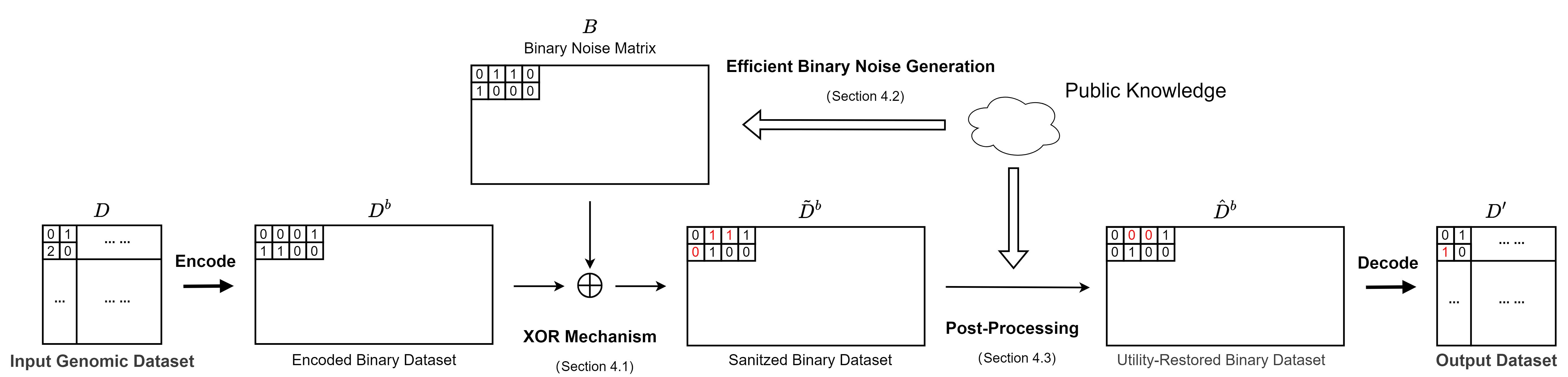
Figure 1: The system workflow. In the first stage, the input genomic dataset $D$ is encoded into a binary form $D^{b}$. This binary dataset is then subjected to an XOR operation with binary noise, generated through Efficient Binary Noise Generation (EBNG) by considering inherited correlations from public reference. In the second stage, we utilize public Minor Allele Frequencies (MAFs) to enhance the data utility of the noisy dataset $\hat{D^{b}}$ and finally share the decoded dataset $D^{\prime}$.

3.1 System Model

In our system, we consider two key parties: the researcher and the verifier. The researcher, discovering GWAS research findings from a local genomic dataset, faces the challenge of potentially reporting incorrect results due to unintentional errors, such as computational errors, during experiments. The researcher would share the entire research dataset along with the findings for external validation; however, direct sharing of genomic datasets raises privacy concerns. Thus, the researcher opts to sanitize the dataset using a privacy-preserving scheme before sharing it.

The verifier, who may be a reviewer in a peer review process or any other researcher seeking to validate results, aims to reproduce the researcher’s experiments using the sanitized dataset. The verifier may utilize public information during the GWAS validation. Aware that the dataset has been distorted with noise for privacy reasons, the verifier anticipates some discrepancies between their and the original results. For instance, if the researcher’s finding suggests that the 100 most significant SNPs are related to a certain trait, determined by the $\chi^{2}$ test or the odds ratio test, the verfier might opt for a more flexible boundary in their analysis. In particular, they might examine the presence of these 100 SNPs exhibiting within the top 120 SNPs in the sanitized dataset instead. This proportion of originally significant SNPs retained within this expanded scope is termed the SNP retention ratio. If this ratio exceeds a certain threshold, the finding is deemed reliable. Otherwise, the verifier might call for further investigation or request more detailed information, subject to IRB approval.

3.2 Genomic Dataset Sharing Workflow

Our proposed workflow, depicted in Figure 1, is motivated by two major concerns. Firstly, we aim to ensure differential privacy and mitigate privacy risks by injecting noise into the original genomic dataset. However, differentially private mechanisms often compromise data utility by distorting an execssive number of data points, which can significantly alter GWAS outcomes and obstruct the verifier’s ability to validate the results. Therefore, we employ a post-processing strategy to restore the data utility of the noisy dataset, rendering it suitable for GWAS outcome validation.

During the data perturbation stage, we first encode the genomic dataset into a binary matrix. Each SNP is represented using two bits while considering the biological property (discussed in Section 4.1). We then implement a noise sampling scheme, an adaptation of the XOR mechanism [24], optimzed for efficient generation of large datasets. This scheme generates a noisy version of the binary matrix while considering inherent correlations among SNPs from publicly available datasets. In the utility restoration stage, we address the utility degradation caused by noise addition. We develop a post-processing technique focused on enhancing the GWAS utility distorted in the first stage. This involves aligning the Minor Allele Frequencies (MAFs) of the noisy dataset with those in a public dataset by selectively flipping allele values. Following this, we decode the altered dataset back into genomic space and make it available to verifiers for validation.

3.3 Threat Model

In our framework, we assume that the researcher is honest yet cautious, holding the original genomic dataset without sharing it directly. Meanwhile, an honest researcher may still unintentionally provide incorrect GWAS outcomes due to computational errors, which could mislead other researchers. Our scheme aims to address this issue by offering a means to reproduce and validate GWAS experiments, enhancing their reliability.

Note that our scope does not extend to scenarios involving a malicious researcher who might intentionally fabricate datasets to report false results. Deliberately creating and using synthetic datasets to produce inaccurate findings poses a challenge that is nearly impossible in most data analysis contexts, not only in GWAS. In this case, only those with direct access to the original data can validate the authenticity of research finding. Moreover, the ethical implications and potential consequence of using fabricated datasets – such as damage to the researcher’s credibility and reputation from funding agencies – serve as strong deterrents against such misconduct.

On the other hand, we assume that the verifier may be malicious and curious about the original dataset. Such a malicious verifier, acting as an attacker, may use membership inference attacks (MIAs) to determine if an individual (the victim) is part of the shared dataset or not. Since individuals in a genomic dataset often share an attribute (e.g., trait or disease), linking the victim to the dataset could also associate them with that attribute. For instance, the researcher shares a dataset consisting of heart disease patients. An attacker could use the published research findings and the shared dataset to predict the target’s presence in the dataset. If the analysis indicates that the target is likely a member, the attacker could infer a potential association of the individual with heart-related diseases.

We assume that the attacker has access to two key piceces of information: (i) the shared dataset from the researcher, and (ii) the specific trait/disease of the individuals in the dataset, e.g., heart disease in the previous example. In addition, the attacker can exploit auxiliary knowledge to launch MIAs by constructing a reference dataset of individuals without the trait/disease (e.g. from the 1000 Genomes project [1]). We consider the following MIAs: 1) Hamming distance-based test (HDT) [21], and a range of machine learning-based attacks including 2) decision tree, 3) random forest, 4) XGBoost [13], and 5) Support Vector Machine [14]. More details will be deferred to Section 5.3.3.

4 Methodology

In this section, we present our scheme in detail. In Section 4.1, we discuss how to generate a noise matrix with inherent correlations among SNPs and apply it to a genomic dataset. In Section 4.2, we present our new noise generation scheme. In Section 4.3, we explain how we restore GWAS reproducibility using statistical information from public sources.

4.1 Genomic Dataset Perturbation

Existing methods are not effective for genomic data due to two primary reasons: they either exhibit high time complexity [28, 47] or fail to appropriately address the inherited correlation among SNPs [25], leading to significant utility loss, as evidenced by our preliminary experiments. We overcome these challenges by converting genomic datasets into binary space. Specifically, we encode each SNP value to 2 bits according to the conversion metric shown in Table III and generate a binary version of the genomic dataset $D^{b}\in\{0,1\}^{n\times 2m}$. It is important to note that this binary representation of SNPs is consistent with their biological characteristics (refer to Section 2.1). As detailed in Section 2.2, SNP data have three values (0, 1 and 2) that indicate the number of minor alleles in a gene. Each allele, inherited from one parent, contributes to the SNP value: ‘00’ for value 0 (no minor allele), ‘01’ for value 1 (one minor allele), and ‘11’ for value 2 (both parents with a minor allele). The binary matrix resulting from this encoding effectively simulates the allele distribution in the geomic sequence. Therefore, flipping one binary value in the binary dataset is analogous to flipping one allele, thus maintaining biological consistency in our data representation.

TABLE III: Encoding SNP Values to Binary Format

Genomic Value	Binary Encoding
0	00
1	01
2	11

After encoding the SNPs into binary bits, we implement the XOR mechanism [24] to perturb the binarized SNP dataset. The perturbation can be represented as $\tilde{D}^{b}=D^{b}\oplus B$, where $D^{b}$ is the original binary SNP dataset, and $\tilde{D}^{b}$ is perturbed outcome. The operator $\oplus$ indicates the XOR operation, and $B\in\{0,1\}^{n\times 2m}$ is the binary noise matrix, sampled from the matrix-valued Bernoulli distribution.

The parameters of this distribution are calibrated with respect to the privacy budget $\epsilon$ and the sensitivity $s_{f}$ of the binary encoding between $D$ and $\hat{D}$ (denoted as $D\sim\hat{D}$), where $D\sim\hat{D}$ implies that the datasets are neighboring genomic datasets differing by one individual’s genomic record. Mathematically, the sensitivity is defined as:

$$s_{f}=\sup_{D,\hat{D}}\|D^{b}\oplus{\hat{D}}^{b}\|_{F}^{2}.$$ (3)

In this context, $\|\cdot\|_{F}^{2}$ represents the Frobenius norm, and $s_{f}$ quantifies the maximum number of differing entries between $D^{b}$ and $\hat{D}^{b}$.

Motivation of Adopting XOR Mechanism. The XOR mechanism is a good fit for our scenario for two main reasons: (i) it can directly generate a binary noise matrix attributed to the matrix-valued Bernoulli distribution with quadratic exponential dependence structure [31]; and (ii) the dependence structure enables the characterization of various correlations among the encoded SNPs. For instance, the entries of $\operatorname{\bm{\Theta}}$ (see the PDF in Equation 1 in Section 2.4.1) are known as the “feature-association” [24, 31]. They model the correlations between columns of $D^{b}\in\{0,1\}^{n\times 2m}$, which represents the inherent correlations between the SNPs [35]. In addition, the entries of $\operatorname{\bm{\Lambda}}_{ij}$ are known as the “object-association”, and they can model the correlations between rows $i$ and $j$ of $D^{b}$, which represents the kinship [23]. If the genomic dataset contains SNP sequences of family members, $\operatorname{\bm{\Lambda}}_{ij}$ can be derived using Mendel’s law. Given the privacy budget $\epsilon$, by determining the parameters of the distribution ($\operatorname{\bm{\Theta}}$ and $\operatorname{\bm{\Lambda}}_{ij}$) based on the correlations that are obtained from some publicly available genomic datasets of the same nature, we can preserve the potential correlations among the SNP data entries in the shared dataset.

Our considered dataset in Section 5.1 does not contain any family members, therefore, we set $\operatorname{\bm{\Lambda}}_{ij}=\mathbf{0}^{2m\times 2m}$. Then, by invoking Theorem 2.1, we have

$$s_{f}||\boldsymbol{\lambda}(\operatorname{\bm{\Theta}})||_{2}\leq\epsilon,$$ (4)

as a sufficient condition to protect the privacy of genomic dataset without kinship correlations. Hence, we only need to calibrate the value of $\operatorname{\bm{\Theta}}$ to satisfy (4).

To preserve the inherent correlations among the SNPs, we consider a publicly available dataset (which has the same set of SNPs as $D$, e.g., the control group in the case-control setup discussed in Section2.2). We use the log-linear association to model such correlation. In particular, we construct a matrix $\widetilde{\operatorname{\bm{\Theta}}}\in\mathcal{R}^{2m\times 2m}$ with diagonal entries $\widetilde{\theta}_{p,p}$ and non-diagonal entries $\widetilde{\theta}_{p,q}$ ($p\neq q$) calculated as

$$\begin{aligned} &\widetilde{\theta}_{p,p}=\log\frac{\Pr(M_{p}=0)}{\Pr(M_{p}=1)},p\in[1,2m]\\ &\widetilde{\theta}_{p,q}=\log\frac{\Pr(M_{p}=0,M_{q}=1)\Pr(M_{p}=1,M_{q}=0)}{\Pr(M_{p}=1,M_{q}=1)\Pr(M_{p}=0,M_{q}=0)},\end{aligned}$$

where $p,q\in[1,2m],p\neq q$ , $M$ is the binarized version of a publicly available dataset, $\Pr(M_{p}=0)$ is the frequency of the entries in the $p$-th column taking value $0$, and similarly $\Pr(M_{p}=0,M_{q}=1)$ is the frequency of the tuples whose value is $0$ in the $p$-th and $1$ in the $q$-th column. Then, by setting

$$\operatorname{\bm{\Theta}}=\frac{\epsilon_{x}}{s_{f}||\widetilde{\operatorname{\bm{\Theta}}}||_{F}}\widetilde{\operatorname{\bm{\Theta}}},$$ (5)

one can verify the sufficient condition of (4) is satisfied. It is noteworthy that in practice, there is an infinite number of ways to generate the value of $\operatorname{\bm{\Theta}}$ and $\operatorname{\bm{\Lambda}}_{ij}$; as long as the sufficient condition in (2) is satisfied, $\epsilon$-differential privacy can be achieved. In [24], the authors assume that $\operatorname{\bm{\Theta}}$ and $\operatorname{\bm{\Lambda}}_{ij}$ are positive definite matrices and propose to generate them by solving a very complex optimization problem. In this work, we lift their assumption and generate $\operatorname{\bm{\Theta}}$ by considering the biological characteristics of SNPs.

4.2 Efficient Binary Noise Generation

Since the original noise generation of the XOR mechanism is time consuming and impractical for genomic datasets, we introduce a novel scheme, named efficient binary noise generation (EBNG). This scheme is designed to enhance the noise generation process, making it feasible and efficient for use with large-scale genomic data.

We first elaborate our novel sampling scheme to generate noise from a given matrix-valued Bernoulli distribution. First, we review the following lemma which connects the matrix-valued Bernoulli distribution with the multivariate Bernoulli distribution.

Lemma 4.1.

[31] If $\operatorname{\mathcal{B}}\sim{\rm{Ber}}_{N,P}(\operatorname{\bm{\Theta}},\operatorname{\bm{\Lambda}}_{1,2},\cdots,\operatorname{\bm{\Lambda}}_{N-1,N})$, then $\operatorname{\mathbf{b}}={\rm{vec}}(\operatorname{\mathcal{B}}^{T})\in\{0,1\}^{NP\times 1}$ is attributed to a multivariate Bernoulli distribution with parameter $\bm{\Pi}$, i.e., ${\rm{vec}}(\operatorname{\mathcal{B}}^{T})\sim{\rm{Ber}}_{NP}(\bm{\Pi})$, and its PDF is

$$f_{{\rm{vec}}(\operatorname{\mathcal{B}}^{T})}({\rm{vec}}(\operatorname{\mathcal{B}}^{T})=\operatorname{\mathbf{b}})=C(\bm{\Pi})\exp\{\operatorname{\mathbf{b}}^{T}\bm{\Pi}\operatorname{\mathbf{b}}\},$$

the parameter $\bm{\Pi}$ and the normalization constant $C(\bm{\Pi})$ are

$$\bm{\Pi} =\mathbf{I}_{N}\otimes\operatorname{\bm{\Theta}}+\sum_{i=1}^{N}\sum_{j\neq i}^{N}\operatorname{\mathbf{J}}_{ij}\otimes\operatorname{\bm{\Lambda}}_{i,j}$$

$$C(\bm{\Pi}) =\Big{[}\sum_{\operatorname{\mathbf{b}}\in\mathcal{S}}\exp\{\operatorname{\mathbf{b}}^{T}\bm{\Pi}\operatorname{\mathbf{b}}\}\Big{]}^{-1},\quad\mathcal{S}=\{0,1\}^{NP\times 1},$$

where $\otimes$ is the Kronecker tensor product.

As discussed in Section  4.1, for genomic datasets without family members, we have $\operatorname{\bm{\Lambda}}_{ij}=\mathbf{0}$. Thus, we can consider a simple form of the multivariate Bernoulli distribution, i.e.,

$$f_{b}(b=\operatorname{\mathbf{b}})=C(\bm{\Pi})\exp\{\operatorname{\mathbf{b}}^{T}\bm{\Pi}\operatorname{\mathbf{b}}\},\ \bm{\Pi}=\mathbf{I}_{N}\otimes\operatorname{\bm{\Theta}}.$$ (6)

Instead of generating matrix-valued binary noise from $\operatorname{\mathcal{B}}\sim{\rm{Ber}}_{N,P}(\operatorname{\bm{\Theta}},\operatorname{\bm{\Lambda}}_{1,2},\cdots,\operatorname{\bm{\Lambda}}_{N-1,N})$, we generate a vectorized version of it from ${\rm{vec}}(\operatorname{\mathcal{B}}^{T})\sim{\rm{Ber}}_{NP}(\bm{\Pi})$ (with PDF shown in (6)), and then reshape the vector noise back into matrix format to perturb the encoded genomic dataset. However, the normalization constant $C(\bm{\Pi})$ (which is a summation of $2^{NP}$ values) is still intractable. Thus, to avoid the time-consuming Hamiltonian Monte Carlo-based sampling scheme (adopted in [24]), we generate each element in the noise vector separately based on its approximated marginal PDF. In what follows, we first present the noise generation scheme along with the privacy guarantee, and then discuss the difference from the sampling scheme proposed in [24]. The detailed theoretical analysis is deferred to Appendix A.

Definition 3 (Efficient Binary Noise Generation).

Given a genomic dataset $D$ without family members (i.e., with independent records), suppose that each individual has $m$ SNPs (i.e., $P=2m$ SNP bits after encoding). The efficient binary noise generation scheme perturbs the $u$th bit ($u\in[1,2m]$) for each individual with a random binary bit $B_{u}$, and $\Pr[B_{u}=1]$ is calibrated based on the correlation among the SNP bits.

The sufficient condition for the above perturbation to preserve $\epsilon$-differential privacy on the entire genomic dataset $D$ is shown below.

Theorem 4.2.

Let $\operatorname{\bm{\Theta}}$ be the parameter determined in (5), ${\rm SUM}(\operatorname{\bm{\Theta}}_{u})$ is the summation of the $u$th row of $\operatorname{\bm{\Theta}}$, and $\operatorname{\bm{\Theta}}_{u,u}$ is the $u$th diagonal entry of $\operatorname{\bm{\Theta}}$. Define

$$\kappa_{u}=2\times{\rm SUM}(\operatorname{\bm{\Theta}}_{u})-\operatorname{\bm{\Theta}}_{u,u},$$

then, Definition 3 achieves $\epsilon$-differential privacy if

$$\Pr[B_{u}=1]=\begin{cases}\frac{1}{2}&\textit{if}\quad\kappa_{u}>||\lambda(\operatorname{\bm{\Theta}})||_{2}\\ \frac{1}{1+\exp(\kappa_{u})}&\textit{if}\quad\kappa_{u}\leq||\lambda(\operatorname{\bm{\Theta}})||_{2}.\end{cases}$$

Proof.

Please refer to Appendix A for the proof. ∎

4.3 Restoring GWAS Utility via Post-Processing

Efficient binary noise generation introduces an excessive amount of noise to the encoded genomic dataset. This poses a significant challenge for verifiers, as the resultant dataset from the XOR mechanism compromises reliable GWAS outcome validation due to substantial utility loss. To address this, we employ a post-processing strategy that leverages publicly available Minor Allele Frequencies (MAFs) to enhance the dataset’s utility.

MAFs, indicating the frequency of the less common allele in a given population, are crucial in genomic research for understanding genentic diversity and are widly utilized in association studies. These values related to a specific phenotype can be readily obtained from public sources like Allele Frequency Aggregator (ALFA) [38] or calculated from public genomic datasets such as 1000Genome [1] and OpenSNP [4]. Importantly, it is not necessary for these MAF values to exactly match those of the original dataset; our primary goal is to boost utility rather than to recover the original dataset in its entirety.

In our approach, the MAFs from public reference are represented as $\mathcal{M^{r}}=\{\mathcal{M^{r}}_{0},\mathcal{M^{r}}_{1},\dots,\mathcal{M^{r}}_{m}\}$, where $\mathcal{M^{r}}_{j}$ is the MAF of the j-th SNP in objective dataset. We also calculate the MAFs, denoted as $\tilde{\mathcal{M}}$, from the dataset generated in the first stage.

To align the MAF distribution of the noisy dataset $\tilde{D}$ with the publicly available MAFs, we employ an optimal transport approach using the earth moving distance [39]. This method calculates the number of the allele (binary) values in $\tilde{D^{b}}$ that needs to be flipped to closely match $\mathcal{M^{r}}$. After that, we randomly select the corresponding number of values in $\tilde{D^{b}}$ and perform the flipping, thereby aligning the MAF distribution while maintaining the integrity of the dataset.

End-to-end Privacy Guarantee. The efficient binary noise generation satisfies $\epsilon$-differential privacy based on Theorem 4.2. According to Proposition 1, differential privacy is immune to post-processing if the post-processing step does not utilize the private dataset $D$. Therefore, our approach of restoring GWAS utility does not compromise the differential privacy guarantees, and our entire sharing scheme is $\epsilon$-differential privacy.

5 Evaluation

We conducted a comprehensive evaluation of our proposed scheme using three real-life genomic datasets from the OpenSNP project [4]. Since we are the first to share a genomic dataset under privacy-preserving techniques, we introduced a local differential privacy approach using randomized response [25] as a baseline approach for comparison. Our approach’s performance was analyzed from four perspectives: GWAS outcome validation, data utility, privacy analysis against membership inference attacks (MIAs), and time complexity.

Additionally, to provide more data points for utility evaluation, we implemented two existing synthetic approaches: DPSyn [28] and PrivBayes [47]. These methods, recognized as winners of the NIST Differential Privacy Synthetic Data Challenge [3], remain state-of-the-art in dataset sharing. We excluded the championship solution (from Team RMcKenna) due to its hard-coded nature and inapplicability to genomic datasets. However, as discussed, these synthetic methods suffer from high time complexity and are unable to share the entire genomic datasets. Therefore, we set up a relaxed scenario in which only 100 SNPs in each dataset are shared for comparison, allowing us to assess the utility performance of our method compared to these approaches.

5.1 Dataset

We leverage the OpenSNP project [4] to construct sample datasets for evaluation. We select three phenotypes, i.e., lactose intolerance, hair color, and eye color. The lactose intolerance dataset includes $9091$ SNPs of $60$ individuals with lactose intolerance. The hair color dataset contains $9686$ SNPs of $60$ individuals who has dark hair. The eye color data set is larger with $28396$ SNPs among $401$ individuals with brown eyes. we build a reference dataset for each phenotype in which the SNPs align with the target dataset to be shared. Additionally, a reference dataset for each phenotype was built from the rest of the OpenSNP project.

5.2 Ethical Considerations

In our study, we utilize existing public genomic datasets to extract inherent correlations between SNPs in the noise generation step (Section 4.2) and leverage the publicly available minor allele frequencies (MAFs) to perform utility restoration (Section 4.3). While these datasets are public accessible and have been previously cleared for use in research, we recognize the importance of addressing ethical considerations in our work.

In particular, we ensure that the use of these datasets aligns with their intended purposes as defined by the original data providers. Our methodologies and objectives are consistent with the terms under which these datasets were made public. Our approach, focused on maintaining the anonymity intergral to these datasets, avoids any attempts at reidentification and strictly follows protocols to prevent de-anonymization. Meanwhile, our work does not involve direct interaction with human participants, thus significantly reducing ethical risks commonly associated with primary data collection. We adhere to recognized standards for secondary data usage, and continually stay informed about ethical guidelines and best practices in genomic research to ensure ongoing compliance.

5.3 Evaluation Metrics

Here, we introduce the evaluation metrics used in the experiments, i.e., GWAS outcome validation, data utility, and robustness against MIAs.

5.3.1 GWAS Outcome Validation

A researcher, in a honest setting, may unintentionally report inaccurate SNPs as GWAS outcomes. We model this error using column shifting, where a correct GWAS finding reports the most significant $\omega\cdot m$ SNPs in the dataset, with $\omega$ being the percentage of interest and $m$ the total number of SNPs. When column shifting occurs, the researcher, instead of reporting the top significant $\omega\cdot m$ SNPs, claims the top $\left\lfloor{\omega\cdot m\cdot\delta+1}\right\rfloor$ to $\left\lfloor{\omega\cdot m\cdot(1+\delta)}\right\rfloor$ SNPs to be the research finding. Here, $\delta$ signifies the shifting factor that models the degree of column shifting. For instance, consider a list $[SNP_{1},SNP_{2},\cdots,SNP_{10}]$ of $10$ SNPs, ranked by statistical significance from highest to lowest), with $\omega=0.2$. Under correct conditions, the significant findings would be $[SNP_{1},SNP_{2}]$. However, with a column shift of $\delta=0.5$, the actual research result would become $[SNP_{2},SNP_{3}]$. For a shift of $\delta=1.0$, the findings would be $[SNP_{3},SNP_{4}]$. The larger the $\delta$, the greater the shift, with $\delta\geq 1.0$ indicating that none of the truly significant SNPs are reported.

The validiation setup is outlined as follows. As detailed in Section 3.1, a verifier acknowledges that the noise introduce during the scheme inevitably causes deviations from the original results, and thus a relaxed metric is employed to validate research findings reported by the researcher. we replicate the GWAS experiments conducted by the researcher, obtain the ranking of SNPs based on statistical significance, and then assess the proportion of the original top $\left\lfloor{\omega\times m}\right\rfloor$ SNPs that remain among the top $\left\lfloor{\frac{\omega}{\zeta}\times m}\right\rfloor$ most significant SNPs in the shared dataset, where $\zeta$ represents the tolerance factor. This proportion is referred as the SNP retention ratio. During validation, if the retention ratio is high, the verifier, trusting the researcher, considers the reported GWAS findings to be accurately reproducible. Conversely, a low retention ratio raises suspicion and may prompt further investigation. Ideally, the verifier should be capable of identifying even minor discrepancies (i.e., small shifts) with high confidence. In Section 5.5, we demonstrate that our proposed scheme effectively identifies such minor errors more accurately than other existing methods.

For GWAS, we focus on two statistics, i.e., the $\chi^{2}$ test and the odds ratio test. The $\chi^{2}$ test, a statistical method, assesses the significance of differences in frequencies between two groups. Specifically, it computes a $\chi^{2}$ statistic that reflects the discrepancy between observed and expected frequencies, i.e., in the shared dataset and the reference dataset, respectively, under the null hypothesis of no association between the phenotype/disease and the SNP position. A higher $\chi^{2}$ value indicates a greate deviation from the null hypothesis, suggesting a significant association.

The odds ratio test, on the other hand, quantifies associations between a phenotype/disease and a specific SNP position using the ratio of the odds. We first calculate the odds ratio as shown in Equation 7.

$$OR=\frac{(S_{1}+S_{2})/(R_{1}+R_{2})}{S_{0}/R_{0}}=\frac{R_{0}(S_{1}+S_{2})}{S_{0}(R_{1}+R_{2})}.$$ (7)

Next, we calculate the $95\%$ confidence interval as $\exp(\ln{(OR)}\pm 1.96\times SE\{\ln{(OR)}\})$, where $SE\{\ln{(OR)}\}$ is defined as $\sqrt{\frac{1}{S_{1}+S_{2}}+\frac{1}{S_{0}}+\frac{1}{R_{1}+R_{2}}+\frac{1}{R_{0}}}$. In this context, $\exp(\cdot)$ represents the exponential function and $SE(\cdot)$ is the standard error of the log odds ratio. Following this, the standard normal deviation, or $z$-value, is computed as $\frac{\ln{(OR)}}{SE\{\ln{(OR)}\}}$, and the $p$-value is the area of the normal distribution outside $\pm z$.

5.3.2 Data Utility

In addition to our primary goal, we evaluate the performance of the proposed scheme using data utility metrics for various data analysis tasks. We employ metrics such as average point error, average sample error, mean error, and variance error. These metrics indicate the extent to which the integrity and statistical properties of the original dataset are maintained when shared with other researchers. The following details each metric.

Average Point Error

Average point error denotes the entry-level discrepancy between two datasets. Given two datasets $D$ and $D^{*}$ of the same dimensions $n\times m$, we determine the number of mismatched entries and define the point error as

$$Error_{p}=\left({{\sum}_{i}^{n}{\sum}_{j}^{m}\textbf{1}_{D_{ij}\neq D^{*}_{ij}}}\right)\Bigg{/}{(n\times m)}.$$ (8)

Average Sample Error

Average sample error measures the distance between each corresponding samples in two datasets. We calculate this using the $l_{1}$ norm, which represents the sum of absolute differences between each sample pair, normalized by the number of SNPs in the datasets, i.e.,

$$Error_{s}=\left({\sum_{i}^{n}\sum_{j}^{m}|D_{ij}-D^{*}_{ij}|}\right)\Bigg{/}{(n\times m)}.$$ (9)

Mean and Variance Error

In addition to the previous metrics, we assess the mean and variance error between the datasets, which are crucial indicators of data fidelity. These errors are measured as the absolute differences in mean and variance values within the SNP domain, compromising values $\{0,1,2\}$.

5.3.3 Robustness against against MIAs

To evaluate privacy protection against MIAs, we adhere to the threat model in Section 3.3 and employed multiple attacks, including the Hamming distance test, likelihood ratio test, and various machine learning-based MIAs. We use recall as the accuracy metric since we only focus on protecting the individuals with a trait/disease in the shared dataset. For each machine learing-based MIA, we train a separate model using a balanced sample of individuals from both the shared dataset and a reference dataset. Recall is then evaluated using the remaining individual in the original, unperturbed version of the shared dataset. The details of the attack strategies employed are outlined below.

5.3.4 Hamming Distance Test (HDT)

The Hamming distance test (HDT) is considered one of the most powerful MIAs against genomic datasets [21]. It leverages the pairwise Hamming distance between genomic sequences in the case group (received from the researcher and subjected to perturbation for privacy guarantees) and in the control group (i.e., constructed from publicly available datasets). Specifically, for each individual $i$ in the shared dataset (i.e., the case group), the malicious client calculates the Hamming distances between individual $i$’ and all individuals in the reference dataset (i.e., the control group), then records the minimum Hamming distance for individual $i$. The malicious client collects all these minimum Hamming for individuals in the case group and selects a threshold $\gamma_{h}$ following $5\%$ false positive rate. When identifying a victim, the malicious client calculates the minimum Hamming distance between the victim’s sequences and all individuals in the control group. If the minimum Hamming distance is lower than the threshold $\gamma_{h}$, the target victim is deemed a member of the case group, and otherwise not.

5.3.5 Machine Learning (ML)-based MIAs

We assume that the attacker uses the following machine learning-based MIAs to perform inference: decision tree (DT), random forest (RF) [37], support vector machine (SVM) [36], and XGBoost [13]. However, considering the limited sample size in two datasets (i.e., lactose intolerance and hair color, each with only 60 samples), we have decided to exclude support vector machine and XGBoost from the analysis for these smaller datasets. This decision is based on the recognition that SVM and XGBoost typically require larger datasets to achieve optimally performance and may not be as effective in scenarios where data availability is limited.

5.4 Experiment Setup

Unless specified otherwise, the following parameters are consistently employed in our experiments. We have set the privacy budget $\epsilon$ to range from $\{1,10,100,1000,10000\}$ for our approach and all comparative methods. It is important to note that, as we are sharing a genomic dataset containing over 9,000 of SNPs, which translates to a sensitivity of 18,000 after encoding, the privacy budget allocated to each SNP is relatively small, thereby satisfying corresponding privacy requirements. The detailed experimental validation of this aspect is presented in Section 5.7.

For the GWAS outcomes, we consider the top $\omega=0.01$ SNPs as significant. The tolerance factor $\zeta=0.7$ for GWAS validation, and the shifting factor $\delta$ is chosen from the range $[0,1.0]$. To ensure robustness, we generate $10$ copies of each dataset using each dataset sharing scheme. Each experiment is conducted in a single trial, and the average results are reported. In the graphical representations, shadowed regions indicate the $95\%$ confidence interval.

In addressing the high dimensionality of the input features (SNPs) for machine learning-based MIAs, we have implemented dimension reduction using Principal Component Analysis (PCA) and retain only the top 10 principal components. However, it’s important to note that for the Hamming distance test, we still use the shared datasets without PCA as these methods are specifically designed for genomic dastasets and optimally function with the complete data.

5.5 Detecting Errors of GWAS Outcomes

We show the experiment results of detecting GWAS outcome errors.

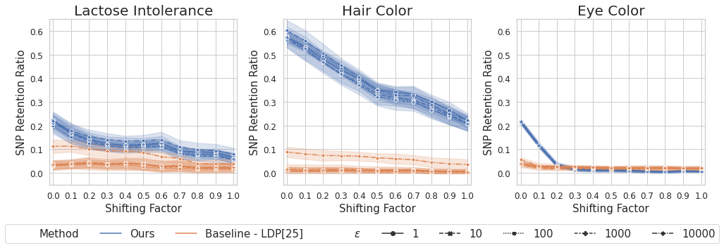
Figure 2: Comparison of error detection of the $\chi^{2}$ test across three phenotypes: lactose intolerance, hair color, and eye color, between our approach and Local Differential Privacy (LDP) [25]. Our scheme shows a better ability to identify slight errors, although results vary by dataset, while LDP shows limited effectiveness in detecting significant errors.

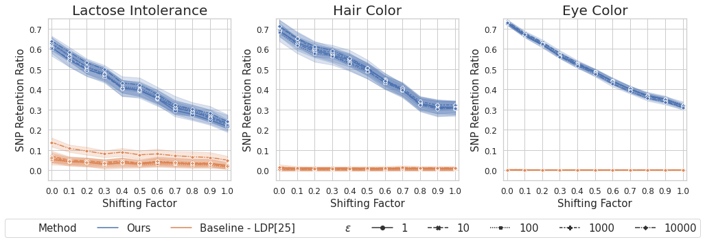
Figure 3: Comparison of error detection of the odds ratio test across three phenotypes: lactose intolerance, hair color, and eye color, between our approach and Local Differential Privacy (LDP) [25]. Our scheme consistently show strong performance in identifying minor errors, whereas LDP fails to identify more significant errors.

5.5.1 $\chi^{2}$ Test

In Figure 2, we copmare our approach with LDP [25] across three datasets. To interpret the figures in our comparison, focus on the difference in SNP retention ratio between the ideal scenario (shifting factor = 0, indicating no error) and situations with varying error levels (modeled by different shifting factors). A greater discrepancy of SNP retention ratio signifies a better capability to detect errors. We demonstrate that our method exhibits a more substantial difference in SNP retention ratios as the shifting factor increases, unlike the nearly flat lines of LDP. However, the results vary by dataset. For instance, the eye color dataset shows a signficant decrease in retention ratios for small shifts, suggesting high sensitivity to errors. Conversely, the lactose intolerance dataset shows small changes and higher variance, presenting challenges in error detection. Acknowledging this limitation, we aim to address it in future research.

5.5.2 Odds Ratio Test

Contrary to the $\chi_{2}$ test, the results of the odds ratio test is more consistent and robust across all datasets. Our scheme demonstrated an ideal SNP retention ratio of around 0.7 for each dataset, with a significant decrease as the shifting factor increases. In contrast, LDP displays limited sensitivity in error detection, characterized by a lower ideal SNP retention ratio and less pronounced slopes in the figures. These observations support our claim that our scheme possesses better capabilities in detecting errors in GWAS outcomes compared to the existing method.

		Point Error		Sample Error		Mean Error		Variance Error
Dataset	$\epsilon$	Proposed	LDP [25]	Proposed	LDP [25]	Proposed	LDP [25]	Proposed	LDP [25]
Lactose Intolerance	1	0.4113	0.4444	0.4686	0.6175	0.0039	0.4376	0.0470	0.3274
	10	0.4111	0.4445	0.4683	0.6176	0.0039	0.4375	0.0470	0.3272
	100	0.4114	0.4425	0.4686	0.6147	0.0039	0.4352	0.0472	0.3266
	1000	0.4093	0.4281	0.4654	0.5950	0.0039	0.4217	0.0471	0.3224
	10000	0.3872	0.2663	0.4311	0.3700	0.0041	0.2619	0.0481	0.2443
Hair Color	1	0.3649	0.4445	0.4136	0.6136	0.0038	0.4324	0.0117	0.3714
	10	0.3647	0.4444	0.4134	0.6138	0.0038	0.4322	0.0117	0.3711
	100	0.3645	0.4430	0.4131	0.6118	0.0038	0.4312	0.0117	0.3710
	1000	0.3630	0.4283	0.4105	0.5915	0.0038	0.4165	0.0119	0.3655
	10000	0.3440	0.2719	0.3808	0.3755	0.0035	0.2648	0.0134	0.2787
Eye Color	1	0.3476	0.4445	0.3948	0.6222	0.0005	0.4647	0.0294	0.3901
	10	0.3476	0.4445	0.3948	0.6222	0.0005	0.4647	0.0294	0.3902
	100	0.3476	0.4439	0.3947	0.6213	0.0005	0.4640	0.0294	0.3900
	1000	0.3473	0.4392	0.3943	0.6147	0.0005	0.4590	0.0294	0.3883
	10000	0.3454	0.3896	0.3910	0.5453	0.0004	0.4072	0.0295	0.3678

TABLE IV: Data utility comparisons across datasets for our approach versus LDP [25]. The confidence intervals for all results presented in the table are less than 0.001.

5.6 Data Utility

Apart from assessing GWAS reproducibility, we evaluated the performance of our proposed scheme against LDP, using metrics detailed in Section 5.3.2. The results, shown in Table IV with better outcomes in bold, indicate that our scheme surpasses LDP in utility metrics in general for $\epsilon<=1000$. However, for $\epsilon=10000$, LDP shows lower average point and sample errors in the lactose intolerance dataset and hair color dataset. Notably, our scheme significantly outperforms LDP in statistical utility under similar point-wise and sample-wise perturbations levels. All confidence intervals are under 0.001 but are omitted due to space constraints and detailed in Figure V in Appendix B. The utility comparison in a 100-SNP setting against DPSyn and PrivBayes is also included in Appendix B.

5.7 Robustness Against Membership Inference Attacks

In this section, we evaluate the robustness of our scheme against membership inference attacks (MIAs) compared with LDP across three datasets. Following the methods outlined in Section 3.3, we evaluate our scheme against Hamming distance test(HDT) [21] and multiple machine learning-based MIAs, including decision tree, random forest, XGBoost [13], and Support Vector Machine [14]. We first show the experiment results by highlighting the maximum attack power among all MIAs in Figure 4. The results reveal LDP’s significant vulnerability, with $100\%$ inference power, while our scheme shows markedly lower vulnerability - 0.55, 0.66, and 0.59 for lactose intolerance, hair color, and eye color datasets, respectively. This indicates our scheme’s better resistance over LDP against membership inference attacks. Detailed analyses of each MIA type follow.

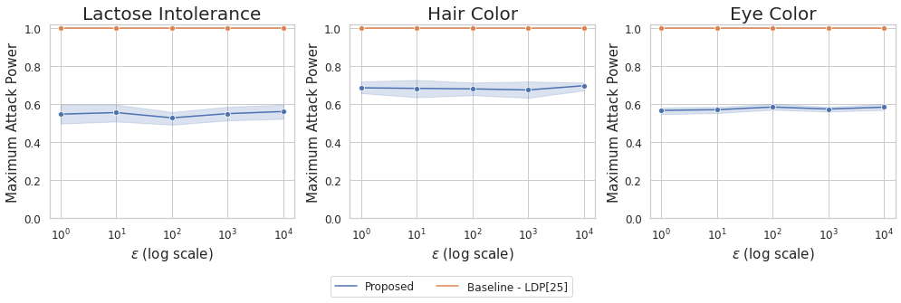
Figure 4: Comparative analysis of maximum attack power in MIAs between our approach and local differential privacy (LDP) [25] across three datasets. Our scheme clearly outperforms LDP in all evaluated datasets.

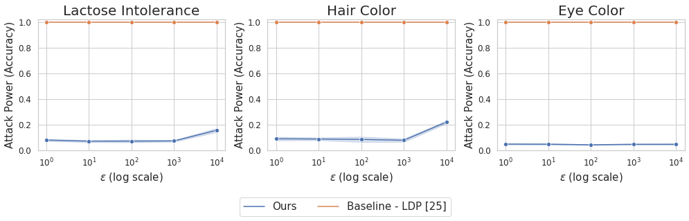
Figure 5: Comparison of our approach and local differential priavcy (LDP) [25] against Hamming distance tests across three datasets. Our scheme maintains attack power below 0.21, while LDP consistently exhibits $100\%$ inference power across in all datasets.

5.7.1 Hamming Distance Test

The experimental findings, illustrated in Figure 5, reveal that our scheme effectively limits the attack power of Hamming Distance Tests to below 0.21, with the peak occurring at $\epsilon=10,000$ in the hair color dataset. In sharp contrast, these tests achieve a consistent $100\%$ inference power against LDP across all tested scenarios. This significant disparity highlights the vulnerability of sensitive genomic datasets when shared using local differential privacy and emphasizes the robustness of our approach in preventing such attacks.

5.7.2 Machine Learning-Based MIAs

In Figure 6, we present our scheme’s performance against machine learning-based MIAs using the eye dataset, chosen for its relatively high sample size of 401, compared to 60 in the other datasets. While acknowledging the limitations of sample size, these results offer insights into our scheme’s protective measures. Both our method and LDP demonstrate robust defense against these MIAs in the eye dataset. Additional results for other datasets are detailed in Appendix B. Notably, in the hair color dataset, SVM-based attacks show a $66\%$ success rate, likely due to the smaller sample size, while other results hover around $60\%$.

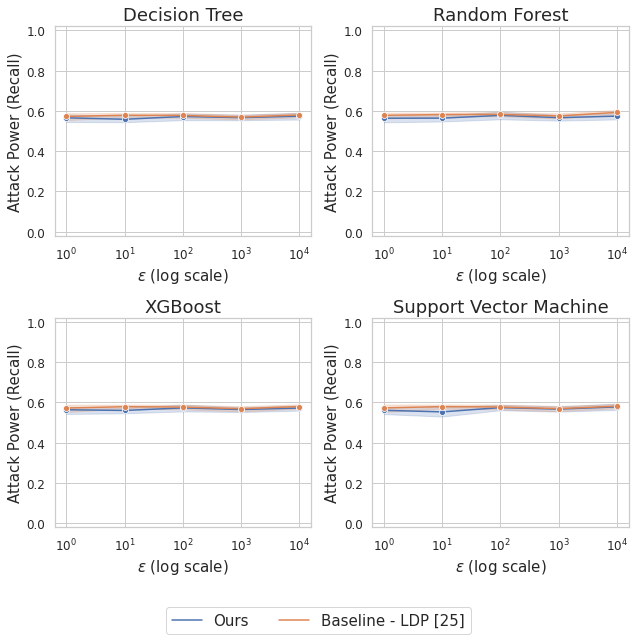
Figure 6: Comparison of robustness of our approach and local differential privacy (LDP) [25] against machine learning-based MIAs on the eye color dataset, with both methods maintaining an attack power of approximately $60\%$.

5.8 Analysis of Time Cost

Figure 7: Comparison of time complexity among our proposed scheme, LDP [25], DPSyn [28], and PrivBayes [47].

We compare the time complexity among our scheme, local differential privacy (LDP) [25], DPSyn [28], and PrivBayes [47], on the lactose intolerance dataset. The results are shown in Figure 7. We observe that our scheme and LDP share similar performance, with our scheme slightly better when number of SNPs is less than 2,000 and LDP outperforms otherwise. The two synthetic methods, i.e., DPSyn and PrivBayes, suffer from high time complexity when the SNP number reaches around 150. This proves that our scheme is time efficient compared with the synthetic methods, while achieving higher privacy protection agains MIAs by combining the results in Section 5.7.

6 Related Work

We discuss related work from three aspects: reproducibility, privacy-preserving dataset sharing, and genomic privacy.

6.1 Reproducibility

Reproducibility ensures that experiment results are consistent in the same setting (e.g., input data and methods), which allows research quality assessment [19] and benefits the development of scientific knowledge [29]. To achieve this, researchers typically share datasets used in their research such that everyone can reconstruct the same experiments and validate their results. Some examples of these datasets include ImageNet [40] and the Iris dataset [18]. However, certain datasets such as genomic and location datasets, may contain sensitive data, and basic anonymization techniques such as hiding identifiable information may not be enough to prevent adversaries from accessing personal information [15]. In this paper, we solve this problem by proposing a differentially-private scheme that shares genomic datasets with high data utility (when the dataset receiver wants to reproduce a GWAS study that has been conducted using the original version of the corresponding dataset) and privacy.

6.2 Privacy-Preserving Dataset Sharing

Differential privacy has become the gold standard for releasing aggregated statistics in a privacy-preserving way. Solutions to achieve differential privacy introduce calibrated noise to the query results, and thus prevent an attacker from gaining excessive information by observing them. Quite a few works have applied differential privacy to share/release datasets. For example, Chanyaswad et al. [12] apply Gaussian noises in matrix format to sanitize a numerical dataset represented as a table. Ji et al. [24] develop the XOR mechanism to release a binary dataset by using noise attributed to the matrix-valued Bernoulli distribution. Andrés et al. [5] consider the release of geolocation datasets by using Laplace noises and achieving geo-indistinguishability (a variant of differential privacy).

Meanwhile, there are also attempts to share datasets by synthesizing them under differential privacy guarantees. For example, Li et al. [28] propose a scheme that generates synthetic datasets by concerning pairwise marginal distribution of features and auxiliary information. Zhang et al. [47] synthesize datasets using Bayesian networks, where conditional probabilities are noisy and protected under differential privacy. Gursoy et al. [20] release synthetic datasets of location trajectories by designing an algorithm that combines four noisy features extracted from the original dataset.

6.3 Genomic Privacy

Genomic privacy has become one of the most interesting topics after several papers reveal privacy concerns for genomic data. Lin et al. [30] claim that $75$ independent SNPs are enough to distinguish one individual from others. Homer et al. [22] successfully determine the presence of a victim in a group (e.g. having the same phenotype) by analyzing aggregate statistics and victim genomic data. Encryption-based approaches[6, 9] are often inefficient concerning computational and communication costs, so the implementation of such approaches is hardly practical. Instead, differential privacy is heavily adopted. Uhler et al. [43] propose a method to release GWAS statistics (e.g., $\chi^{2}$), and Yu et al. [46] improve this work by allowing an arbitrary number of case and control individuals while considering auxiliary information. Yilmaz et al. [45] consider the correlations between SNPs and propose dependent local differential privacy to release individual genomic records. Yet, it only works for individual genomic sequences and cannot be extended to dataset sharing. Our approach publishes entire genomic datasets under differential privacy with high dataset utility and GWAS statistics.

7 Limitations and Future Work

In this paper, we propose a novel scheme for sharing genomic datasets in a privacy-preserving manner, specifically for GWAS outcome validation. We efficiently adapted the XOR mechanism to generate binary datasets with correlations derived from public references and enhanced data utility using public Minor Allele Frequencies (MAFs). Our approach demonstrates superiority in detecting GWAS outcome errors, data utility, and robustness against membership inference attacks.

However, this work has limitations. It’s tailored only for GWAS reproducibility and not applicable to other genomic studies such as transcriptome-wide association, genetic epidemiology, or gene-environment interaction. Our approach also relies on public reference datasets and MAFs, which may not match exactly or even exist. Additionally, the shared datasets suffer from poor usability due to the added noise. We will explore the feasibility of achieving both privacy and usability in realistic genomic research. Future work will also focus on integrating dataset fingerprinting for liability and privacy assurances in genomic data sharing.

Appendix A Proof of Theorem 4.2

Proof.

In the first step, we bound the marginal probability of each noise bit taking value 1 as follows

$$\Pr[\mathbf{b}_{u}=1] =\sum_{\operatorname{\mathbf{b}}\in\mathcal{S}_{u}}C(\bm{\Pi})\exp\{\operatorname{\mathbf{b}}^{T}\bm{\Pi}\operatorname{\mathbf{b}}\}$$

$$=\frac{\sum_{\operatorname{\mathbf{b}}\in\mathcal{S}_{u}}\exp\{\operatorname{\mathbf{b}}^{T}\bm{\Pi}\operatorname{\mathbf{b}}\}}{\sum_{\operatorname{\mathbf{b}}\in\mathcal{S}}\exp\{\operatorname{\mathbf{b}}^{T}\bm{\Pi}\operatorname{\mathbf{b}}\}}$$

$$\stackrel{{\scriptstyle(a)}}{{=}}\leavevmode\resizebox{328.82706pt}{}{$\frac{\sum_{\operatorname{\mathbf{b}}\in\mathcal{S}_{u}}\exp\{\operatorname{\mathbf{b}}^{T}\bm{\Pi}\operatorname{\mathbf{b}}\}}{\sum_{\operatorname{\mathbf{b}}\in\mathcal{S}_{u}}\exp\{\operatorname{\mathbf{b}}^{T}\bm{\Pi}\operatorname{\mathbf{b}}\}+\sum_{\operatorname{\mathbf{b}}\in\overline{\mathcal{S}_{u}}}\exp\{\operatorname{\mathbf{b}}^{T}\bm{\Pi}\operatorname{\mathbf{b}}\}}$}$$

$$=\frac{1}{1+\frac{\sum_{\operatorname{\mathbf{b}}\in\overline{\mathcal{S}_{u}}}\exp\{\operatorname{\mathbf{b}}^{T}\bm{\Pi}\operatorname{\mathbf{b}}\}}{\sum_{\operatorname{\mathbf{b}}\in\mathcal{S}_{u}}\exp\{\operatorname{\mathbf{b}}^{T}\bm{\Pi}\operatorname{\mathbf{b}}\}}}$$

$$\stackrel{{\scriptstyle(b)}}{{=}}\frac{1}{1+\frac{\sum_{\operatorname{\mathbf{b}}\in\overline{\mathcal{S}_{u}}}\exp\{\operatorname{\mathbf{b}}^{T}\bm{\Pi}\operatorname{\mathbf{b}}\}}{\sum_{\operatorname{\mathbf{b}}\in\overline{\mathcal{S}_{u}}}\exp\left\{(\operatorname{\mathbf{b}}+\boldsymbol{j}_{u})^{T}\bm{\Pi}(\operatorname{\mathbf{b}}+\boldsymbol{j}_{u})\right\}}}$$

$$\stackrel{{\scriptstyle(c)}}{{\leq}}\frac{1}{1+\min_{\operatorname{\mathbf{b}}\in\overline{\mathcal{S}_{u}}}\frac{\exp\{\operatorname{\mathbf{b}}^{T}\bm{\Pi}\operatorname{\mathbf{b}}\}}{\exp\left\{(\operatorname{\mathbf{b}}+\boldsymbol{j}_{u})^{T}\bm{\Pi}(\operatorname{\mathbf{b}}+\boldsymbol{j}_{u})\right\}}}$$

$$\leq\frac{1}{1+\max_{\operatorname{\mathbf{b}}\in\overline{\mathcal{S}_{u}}}\exp\left\{2\boldsymbol{j}_{u}^{T}\bm{\Pi}\operatorname{\mathbf{b}}+\bm{\Pi}_{u,u}\right\}},$$

where in $(a)$, $\overline{\mathcal{S}_{u}}$ is the complementary set of $\mathcal{S}_{u}$, i.e., $\overline{\mathcal{S}_{u}}=\big{\{}\operatorname{\mathbf{b}}|\operatorname{\mathbf{b}}_{u}=0,\operatorname{\mathbf{b}}_{v}\in\{0,1\},\forall v\in\{1,2,\cdots,NP\},v\neq u\big{\}}.$ $(b)$ is because by defining the one-hot vector $\boldsymbol{j}_{u}\in\{0,1\}^{NP\times 1}$ that only has 1 at the $u$th position, and 0 at all the other positions. Then, $\forall\operatorname{\mathbf{b}}\in\overline{\mathcal{S}_{u}}$, we have $\operatorname{\mathbf{b}}+\boldsymbol{j}_{u}\in\mathcal{S}_{u}$. $(c)$ is because $\frac{\sum x_{i}}{\sum y_{i}}\geq\min_{i}\frac{x_{i}}{y_{i}}$ for positive sequences $x_{i}$ and $y_{i}$, and in $(c)$ $\bm{\Pi}_{u,u}$ represents the entry of $\bm{\Pi}$ in the $u$th row and $u$th column.

In step 2, we proceed to calculate the maximum value, i.e.,

In particular, we observe that $\boldsymbol{j}_{u}^{T}\bm{\Pi}$ represents the $u$th row of $\bm{\Pi}$, thus $\max_{\operatorname{\mathbf{b}}\in\overline{\mathcal{S}_{u}}}\boldsymbol{j}_{u}^{T}\bm{\Pi}\operatorname{\mathbf{b}}$ corresponds to the summation of all positive values in the $u$th row of $\bm{\Pi}$ except for $\bm{\Pi}_{u,u}$ (since $\operatorname{\mathbf{b}}_{u}=0$). By denoting the maximum value as $\kappa_{u}$, we have

$$\kappa_{u}=2\times{\rm Sum}(\bm{\Pi}_{u})-\bm{\Pi}_{u,u}$$

In step 3, we prove that the probability ratio of the outputs of the efficient genomic dataset perturbation is bounded by $\exp(\epsilon)$. W.l.o.g., suppose $D$ and $D^{\prime}$ only differ by the SNP sequence of the first individual, and let $\boldsymbol{d}$ and $\boldsymbol{d}^{\prime}$ be the encoded SNP sequences of the first individual in $D$ and $D^{\prime}$, respectively.

$$\begin{aligned} &\ln\left(\frac{\prod_{u}\Pr(\boldsymbol{d}_{u}\oplus B_{u}=O_{u})}{\prod_{u}\Pr(\boldsymbol{d}^{\prime}_{u}\oplus B^{\prime}_{u}=O_{u})}\right)\\ =&\sum_{u}\ln\frac{\Pr(B_{u}=O_{u}\oplus\boldsymbol{d}_{u})}{\Pr(B^{\prime}_{u}=O_{u}\oplus\boldsymbol{d}^{\prime}_{u})}\\ =&\sum_{u}\ln\frac{\Pr(B_{u}=1)^{O_{u}\oplus\boldsymbol{d}_{u}}(1-\Pr(B_{u}=1))^{1-(O_{u}\oplus\boldsymbol{d}_{u})}}{\Pr(B_{u}^{\prime}=1)^{O_{u}\oplus\boldsymbol{d}_{u}^{\prime}}(1-\Pr(B_{u}^{\prime}=1))^{1-(O_{u}\oplus\boldsymbol{d}_{u}^{\prime})}}\\ =&\sum_{u}[(O_{u}\oplus\boldsymbol{d}_{u})-(O_{u}\oplus\boldsymbol{d}_{u}^{\prime})]\ln\Pr(B_{u}=1)+\\ &\quad\ \ [(O_{u}\oplus\boldsymbol{d}_{u}^{\prime})-(O_{u}\oplus\boldsymbol{d}_{u})]\ln(1-\Pr(B_{u}=1))\\ =&\Biggl{(}\sum_{\{u:\kappa_{u}>||\lambda(\operatorname{\bm{\Theta}})||\}}[(O_{u}\oplus\boldsymbol{d}_{u})-(O_{u}\oplus\boldsymbol{d}_{u}^{\prime})]\ln\Pr(B_{u}=1)+\\ &\quad\ \ [(O_{u}\oplus\boldsymbol{d}_{u}^{\prime})-(O_{u}\oplus\boldsymbol{d}_{u})]\ln(1-\Pr(B_{u}=1))\Biggl{)}\\ +&\Biggl{(}\sum_{\{u:\kappa_{u}\leq||\lambda(\operatorname{\bm{\Theta}})||\}}[(O_{u}\oplus\boldsymbol{d}_{u})-(O_{u}\oplus\boldsymbol{d}_{u}^{\prime})]\ln\Pr(B_{u}=1)+\\ &\quad\ \ [(O_{u}\oplus\boldsymbol{d}_{u}^{\prime})-(O_{u}\oplus\boldsymbol{d}_{u})]\ln(1-\Pr(B_{u}=1))\Biggl{)}\\ \stackrel{{\scriptstyle(a)}}{{=}}&\sum_{\{u:\kappa_{u}\leq||\lambda(\operatorname{\bm{\Theta}})||\}}[(O_{u}\oplus\boldsymbol{d}_{u})-(O_{u}\oplus\boldsymbol{d}_{u}^{\prime})]\ln\frac{1}{1+\exp(\kappa_{u})}+\\ &\quad\ \ [(O_{u}\oplus\boldsymbol{d}_{u}^{\prime})-(O_{u}\oplus\boldsymbol{d}_{u})]\ln\frac{\exp(\kappa_{u})}{1+\exp(\kappa_{u})}\\ =&\sum_{\{u:\kappa_{u}\leq||\lambda(\operatorname{\bm{\Theta}})||\}}[(O_{u}\oplus\boldsymbol{d}_{u})-(O_{u}\oplus\boldsymbol{d}_{u}^{\prime})]\\ &\qquad\quad\times\left(\ln\frac{1}{1+\exp(\kappa_{u})}-\ln\frac{\exp(\kappa_{u})}{1+\exp(\kappa_{u})}\right)\\ =&\sum_{\{u:\kappa_{u}\leq||\lambda(\operatorname{\bm{\Theta}})||\}}[(O_{u}\oplus\boldsymbol{d}_{u})-(O_{u}\oplus\boldsymbol{d}_{u}^{\prime})]\ln\frac{1}{\exp(\kappa_{u})}\\ \stackrel{{\scriptstyle(b)}}{{=}}&\sum_{\{u:\kappa_{u}\leq||\lambda(\operatorname{\bm{\Theta}})||\}}|2O_{u}-1||\boldsymbol{d}_{u}^{\prime}-\boldsymbol{d}_{u}||\kappa_{u}|\\ \stackrel{{\scriptstyle(c)}}{{<}}&s_{f}||\lambda(\operatorname{\bm{\Theta}})||_{2},\end{aligned}$$

where $(a)$ is because the summation is 0 for $\{u:\kappa_{u}>||\lambda(\operatorname{\bm{\Theta}})||\}$, $(b)$ is because $u\oplus v=(1-u)v+u(1-v)$ for binary $u$ and $v$, and $(c)$ is because the cardinity of set $\{u:\kappa_{u}\leq||\lambda(\operatorname{\bm{\Theta}})||\}$ is at most $s_{f}$. According to (4), we have $s_{f}||\lambda(\operatorname{\bm{\Theta}})||_{2}<\epsilon$. Thus, we complete the proof. ∎

Appendix B Additional Experiment Results on the Lactose Intolerance Dataset and the Hair Color Dataset Against ML-based MIAs

We present the additional experiment results on the lactose intolerance dataset and the hair color dataset against machine learning-based membership inference attacks in Figure 8 and 9.

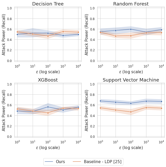
Figure 8: Comparison of robustness of our approach and local differential privacy (LDP) [25] against machine learning-based MIAs on the hair color dataset.

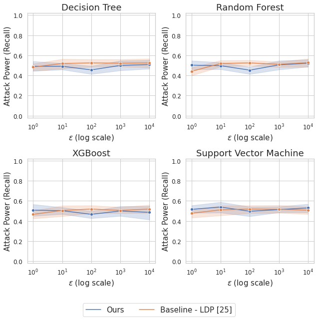
Figure 9: Comparison of robustness of our approach and local differential privacy (LDP) [25] against machine learning-based MIAs on the lactose intolerance dataset.

Appendix C Utility comparison

In our analysis, we present a comprehensive utility comparison of our method alongside DPSyn [28] and PrivBayes [47] across three datasets. This comparison is conducted in two distinct settings: first, by sharing the entire datasets, as detailed in Figure V, and second, by sharing a smaller, toy dataset comprising 100 SNPs, shown in Figure VI.

		Point Error		Sample Error		Mean Error		Variance Error
Dataset	e	Ours	LDP [25]	Ours	LDP [25]	Ours	LDP [25]	Ours	LDP [25]
Lactose	1	0.4113±0.0003	0.4444±0.0004	0.4686±0.0003	0.6175±0.0006	0.0039±0.0000	0.4376±0.0005	0.0470±0.0002	0.3274±0.0003
	10	0.4111±0.0004	0.4445±0.0005	0.4683±0.0004	0.6176±0.0009	0.0039±0.0000	0.4375±0.0008	0.0470±0.0002	0.3272±0.0005
	100	0.4114±0.0002	0.4425±0.0004	0.4686±0.0002	0.6147±0.0008	0.0039±0.0000	0.4352±0.0006	0.0472±0.0002	0.3266±0.0003
	1000	0.4093±0.0003	0.4281±0.0004	0.4654±0.0003	0.5950±0.0006	0.0039±0.0001	0.4217±0.0006	0.0471±0.0002	0.3224±0.0004
	10000	0.3872±0.0004	0.2663±0.0004	0.4311±0.0004	0.3700±0.0006	0.0041±0.0000	0.2619±0.0005	0.0481±0.0002	0.2443±0.0005
Hair	1	0.3649±0.0002	0.4445±0.0005	0.4136±0.0003	0.6136±0.0006	0.0038±0.0001	0.4324±0.0003	0.0117±0.0002	0.3714±0.0003
	10	0.3647±0.0002	0.4444±0.0004	0.4134±0.0003	0.6138±0.0006	0.0038±0.0000	0.4322±0.0007	0.0117±0.0003	0.3711±0.0004
	100	0.3645±0.0003	0.4430±0.0003	0.4131±0.0004	0.6118±0.0004	0.0038±0.0001	0.4312±0.0006	0.0117±0.0001	0.3710±0.0004
	1000	0.3630±0.0002	0.4283±0.0004	0.4105±0.0003	0.5915±0.0006	0.0038±0.0000	0.4165±0.0006	0.0119±0.0002	0.3655±0.0004
	10000	0.3440±0.0003	0.2719±0.0004	0.3808±0.0004	0.3755±0.0006	0.0035±0.0000	0.2648±0.0004	0.0134±0.0003	0.2787±0.0006
Eye	1	0.3476±0.0001	0.4445±0.0001	0.3948±0.0001	0.6222±0.0001	0.0005±0.0000	0.4647±0.0002	0.0294±0.0000	0.3901±0.0000
	10	0.3476±0.0000	0.4445±0.0001	0.3948±0.0001	0.6222±0.0001	0.0005±0.0000	0.4647±0.0001	0.0294±0.0000	0.3902±0.0001
	100	0.3476±0.0000	0.4439±0.0001	0.3947±0.0001	0.6213±0.0001	0.0005±0.0000	0.4640±0.0002	0.0294±0.0001	0.3900±0.0001
	1000	0.3473±0.0000	0.4392±0.0001	0.3943±0.0000	0.6147±0.0002	0.0005±0.0000	0.4590±0.0001	0.0294±0.0000	0.3883±0.0001
	10000	0.3454±0.0000	0.3896±0.0001	0.3910±0.0000	0.5453±0.0001	0.0004±0.0000	0.4072±0.0001	0.0295±0.0001	0.3678±0.0001

TABLE V: Data utility comparisons across datasets for our approach versus LDP [25]. (Full version)

		Point Error			Sample Error			Mean Error			Variance Error
Dataset	e	Ours	DPSyn [28]	PrivBayes [47]	Ours	DPSyn [28]	PrivBayes [47]	Ours	DPSyn [28]	PrivBayes [47]	Ours	DPSyn [28]	PrivBayes [47]
Lactose	1	0.42±0.01	0.65±0.00	0.65±0.01	0.49±0.01	0.88±0.01	0.88±0.01	0.03±0.01	0.61±0.01	0.60±0.01	0.07±0.01	0.30±0.01	0.24±0.02
	10	0.42±0.01	0.65±0.00	0.61±0.01	0.49±0.02	0.88±0.01	0.82±0.01	0.03±0.01	0.61±0.01	0.51±0.01	0.07±0.01	0.30±0.01	0.25±0.01
	100	0.42±0.01	0.65±0.00	0.48±0.01	0.48±0.02	0.88±0.01	0.61±0.01	0.03±0.01	0.61±0.01	0.19±0.01	0.07±0.01	0.30±0.01	0.16±0.01
	1000	0.38±0.06	0.65±0.00	0.42±0.01	0.44±0.07	0.88±0.01	0.50±0.01	0.03±0.01	0.61±0.01	0.03±0.01	0.04±0.01	0.30±0.01	0.03±0.00
	10000	0.36±0.07	0.65±0.00	0.41±0.01	0.43±0.09	0.88±0.01	0.49±0.01	0.03±0.01	0.61±0.01	0.02±0.01	0.03±0.01	0.30±0.01	0.02±0.00
Hair	1	0.44±0.01	0.55±0.02	0.55±0.02	0.51±0.02	0.70±0.02	0.70±0.03	0.03±0.01	0.42±0.02	0.42±0.03	0.01±0.01	0.22±0.01	0.15±0.02
	10	0.44±0.01	0.55±0.02	0.51±0.02	0.51±0.02	0.70±0.02	0.64±0.03	0.03±0.01	0.42±0.02	0.33±0.02	0.02±0.01	0.22±0.01	0.14±0.02
	100	0.44±0.01	0.55±0.02	0.41±0.02	0.51±0.02	0.70±0.02	0.48±0.02	0.03±0.01	0.42±0.02	0.10±0.01	0.01±0.01	0.22±0.01	0.08±0.01
	1000	0.42±0.05	0.55±0.02	0.38±0.02	0.48±0.07	0.70±0.02	0.43±0.02	0.03±0.01	0.42±0.02	0.02±0.01	0.02±0.01	0.22±0.01	0.02±0.01
	10000	0.40±0.08	0.55±0.02	0.37±0.02	0.47±0.09	0.70±0.02	0.43±0.02	0.03±0.01	0.42±0.02	0.01±0.00	0.02±0.01	0.22±0.01	0.01±0.00
Eye	1	0.39±0.01	0.62±0.01	0.60±0.01	0.45±0.02	0.85±0.01	0.81±0.02	0.02±0.01	0.61±0.02	0.56±0.02	0.04±0.01	0.34±0.01	0.28±0.03
	10	0.38±0.01	0.62±0.01	0.44±0.01	0.44±0.02	0.85±0.01	0.56±0.02	0.02±0.01	0.61±0.02	0.22±0.02	0.04±0.01	0.34±0.01	0.21±0.02
	100	0.38±0.02	0.62±0.01	0.35±0.01	0.44±0.02	0.85±0.01	0.42±0.01	0.02±0.01	0.61±0.02	0.03±0.00	0.04±0.01	0.34±0.01	0.03±0.00
	1000	0.37±0.04	0.62±0.01	0.34±0.01	0.42±0.05	0.85±0.01	0.40±0.02	0.02±0.01	0.61±0.02	0.01±0.00	0.05±0.01	0.34±0.01	0.01±0.00
	10000	0.33±0.07	0.62±0.01	0.34±0.01	0.39±0.08	0.85±0.01	0.40±0.01	0.02±0.01	0.61±0.02	0.01±0.00	0.02±0.01	0.34±0.01	0.00±0.00

TABLE VI: Comparison of data utility across datasets with only 100 SNPs for our scheme versus DPSyn [28] and PrivBayes [47].

References

- [1] 1000 genomes. https://www.internationalgenome.org/. [Online; accessed April-12-2023].
- [2] ”what are single nucleotide polymorphisms (snps)?”. https://medlineplus.gov/genetics/understanding/genomicresearch/snp/. [Online; accessed April-12-2023].
- [3] Nist 2018: Differential privacy synthetic data challenge. https://www.nist.gov/ctl/pscr/open-innovation-prize-challenges/past-prize-challenges/2018-differential-privacy-synthetic, 2022. [Online; accessed April-12-2023].
- [4] The opensnp project. https://opensnp.org/, 2022. [Online; accessed April-12-2023].
- [5] Miguel E Andrés, Nicolás E Bordenabe, Konstantinos Chatzikokolakis, and Catuscia Palamidessi. Geo-indistinguishability: Differential privacy for location-based systems. In Proceedings of the 2013 ACM SIGSAC conference on Computer & communications security, pages 901–914, 2013.
- [6] Mikhail J Atallah, Florian Kerschbaum, and Wenliang Du. Secure and private sequence comparisons. In Proceedings of the 2003 ACM Workshop on Privacy in the Electronic Society, pages 39–44, 2003.
- [7] C Glenn Begley and John PA Ioannidis. Reproducibility in science: improving the standard for basic and preclinical research. Circulation research, 116(1):116–126, 2015.
- [8] Rebecca A Betensky and Alice S Whittemore. An analysis of correlated multivariate binary data: Application to familial cancers of the ovary and breast. Journal of the Royal Statistical Society: Series C (Applied Statistics), 45(4):411–429, 1996.
- [9] Marina Blanton, Mikhail J Atallah, Keith B Frikken, and Qutaibah Malluhi. Secure and efficient outsourcing of sequence comparisons. In European Symposium on Research in Computer Security, pages 505–522. Springer, 2012.
- [10] Rita M Cantor, Kenneth Lange, and Janet S Sinsheimer. Prioritizing gwas results: a review of statistical methods and recommendations for their application. The American Journal of Human Genetics, 86(1):6–22, 2010.
- [11] Christopher S Carlson, Michael A Eberle, Mark J Rieder, Joshua D Smith, Leonid Kruglyak, and Deborah A Nickerson. Additional snps and linkage-disequilibrium analyses are necessary for whole-genome association studies in humans. Nature genetics, 33(4):518–521, 2003.
- [12] Thee Chanyaswad, Alex Dytso, H Vincent Poor, and Prateek Mittal. Mvg mechanism: Differential privacy under matrix-valued query. In Proceedings of the 2018 ACM SIGSAC Conference on Computer and Communications Security, pages 230–246, 2018.
- [13] Tianqi Chen and Carlos Guestrin. Xgboost: A scalable tree boosting system. In Proceedings of the 22nd acm sigkdd international conference on knowledge discovery and data mining, pages 785–794, 2016.
- [14] Corinna Cortes and Vladimir Vapnik. Support-vector networks. Machine learning, 20(3):273–297, 1995.
- [15] Yves-Alexandre De Montjoye, César A Hidalgo, Michel Verleysen, and Vincent D Blondel. Unique in the crowd: The privacy bounds of human mobility. Scientific reports, 3(1):1–5, 2013.
- [16] Laramie E Duncan, Michael Ostacher, and Jacob Ballon. How genome-wide association studies (gwas) made traditional candidate gene studies obsolete. Neuropsychopharmacology, 44(9):1518–1523, 2019.
- [17] Cynthia Dwork. Differential privacy: A survey of results. In International conference on theory and applications of models of computation, pages 1–19. Springer, 2008.
- [18] Ronald A Fisher. The use of multiple measurements in taxonomic problems. Annals of eugenics, 7(2):179–188, 1936.
- [19] Steven N Goodman, Daniele Fanelli, and John PA Ioannidis. What does research reproducibility mean? Science translational medicine, 8(341):341ps12–341ps12, 2016.
- [20] Mehmet Emre Gursoy, Ling Liu, Stacey Truex, and Lei Yu. Differentially private and utility preserving publication of trajectory data. IEEE Transactions on Mobile Computing, 18(10):2315–2329, 2018.
- [21] Anisa Halimi, Leonard Dervishi, Erman Ayday, Apostolos Pyrgelis, Juan Ramón Troncoso-Pastoriza, Jean-Pierre Hubaux, Xiaoqian Jiang, and Jaideep Vaidya. Privacy-preserving and efficient verification of the outcome in genome-wide association studies. Proceedings on Privacy Enhancing Technologies, 2022:732–753, 07 2022.
- [22] Nils Homer, Szabolcs Szelinger, Margot Redman, David Duggan, Waibhav Tembe, Jill Muehling, John V Pearson, Dietrich A Stephan, Stanley F Nelson, and David W Craig. Resolving individuals contributing trace amounts of dna to highly complex mixtures using high-density snp genotyping microarrays. PLoS genetics, 4(8):e1000167, 2008.
- [23] Tianxi Ji, Erman Ayday, Emre Yilmaz, and Pan Li. Robust fingerprinting of genomic databases. In 30th International Conference on Intelligent Systems for Molecular Biology, ISMB’21, Oxford, England, 2021. Oxford University Press.
- [24] Tianxi Ji, Pan Li, Emre Yilmaz, Erman Ayday, Yanfang Ye, and Jinyuan Sun. Differentially private binary-and matrix-valued data query: an xor mechanism. Proceedings of the VLDB Endowment, 14(5):849–862, 2021.
- [25] Shiva Prasad Kasiviswanathan, Homin K Lee, Kobbi Nissim, Sofya Raskhodnikova, and Adam Smith. What can we learn privately? SIAM Journal on Computing, 40(3):793–826, 2011.
- [26] Arthur Korte and Ashley Farlow. The advantages and limitations of trait analysis with gwas: a review. Plant methods, 9(1):1–9, 2013.
- [27] Myrto Lefkopoulou, Dirk Moore, and Louise Ryan. The analysis of multiple correlated binary outcomes: application to rodent teratology experiments. Journal of the American Statistical Association, 84(407):810–815, 1989.
- [28] Ninghui Li, Zhikun Zhang, and Tianhao Wang. Dpsyn: Experiences in the nist differential privacy data synthesis challenges. arXiv preprint arXiv:2106.12949, 2021.
- [29] Xihong Lin. Learning Lessons on Reproducibility and Replicability in Large Scale Genome-Wide Association Studies. Harvard Data Science Review, 2(4), dec 16 2020. https://hdsr.mitpress.mit.edu/pub/yosmh9o4.
- [30] Zhen Lin, Art B Owen, and Russ B Altman. Genomic research and human subject privacy, 2004.
- [31] Gianfranco Lovison. A matrix-valued bernoulli distribution. Journal of Multivariate Analysis, 97(7):1573–1585, 2006.
- [32] Wainer Lusoli. Reproducibility of Scientific Results in the EU: Scoping report. Publications Office of the European Union, 2020.
- [33] Adele A Mitchell, Michael E Zwick, Aravinda Chakravarti, and David J Cutler. Discrepancies in dbsnp confirmation rates and allele frequency distributions from varying genotyping error rates and patterns. Bioinformatics, 20(7):1022–1032, 2004.
- [34] Florian Mittag, Michael Römer, and Andreas Zell. Influence of feature encoding and choice of classifier on disease risk prediction in genome-wide association studies. PloS one, 10(8):e0135832, 2015.
- [35] Muhammad Naveed, Erman Ayday, Ellen W Clayton, Jacques Fellay, Carl A Gunter, Jean-Pierre Hubaux, Bradley A Malin, and XiaoFeng Wang. Privacy in the genomic era. ACM Computing Surveys (CSUR), 48(1):1–44, 2015.
- [36] William S Noble. What is a support vector machine? Nature biotechnology, 24(12):1565–1567, 2006.
- [37] Mahesh Pal. Random forest classifier for remote sensing classification. International journal of remote sensing, 26(1):217–222, 2005.
- [38] L Phan, Y Jin, H Zhang, W Qiang, E Shekhtman, D Shao, D Revoe, R Villamarin, E Ivanchenko, M Kimura, et al. Alfa: allele frequency aggregator. National Center for Biotechnology Information, US National Library of Medicine, 10, 2020.
- [39] Yossi Rubner, Carlo Tomasi, and Leonidas J Guibas. A metric for distributions with applications to image databases. In Sixth international conference on computer vision (IEEE Cat. No. 98CH36271), pages 59–66. IEEE, 1998.
- [40] Olga Russakovsky, Jia Deng, Hao Su, Jonathan Krause, Sanjeev Satheesh, Sean Ma, Zhiheng Huang, Andrej Karpathy, Aditya Khosla, Michael Bernstein, Alexander C. Berg, and Li Fei-Fei. ImageNet Large Scale Visual Recognition Challenge. International Journal of Computer Vision (IJCV), 115(3):211–252, 2015.
- [41] Vivian Tam, Nikunj Patel, Michelle Turcotte, Yohan Bossé, Guillaume Paré, and David Meyre. Benefits and limitations of genome-wide association studies. Nature Reviews Genetics, 20(8):467–484, 2019.
- [42] National Academies of Sciences, Engineering, and Medicine et al. Reproducibility and replicability in science. 2019.
- [43] Caroline Uhlerop, Aleksandra Slavković, and Stephen E Fienberg. Privacy-preserving data sharing for genome-wide association studies. The Journal of privacy and confidentiality, 5(1):137, 2013.
- [44] Yonghui Xiao and Li Xiong. Protecting locations with differential privacy under temporal correlations. In Proceedings of the 22nd ACM SIGSAC Conference on Computer and Communications Security, pages 1298–1309, 2015.
- [45] Emre Yilmaz, Tianxi Ji, Erman Ayday, and Pan Li. Genomic data sharing under dependent local differential privacy. In Proceedings of the Twelveth ACM Conference on Data and Application Security and Privacy, pages 77–88, 2022.
- [46] Fei Yu, Stephen E Fienberg, Aleksandra B Slavković, and Caroline Uhler. Scalable privacy-preserving data sharing methodology for genome-wide association studies. Journal of biomedical informatics, 50:133–141, 2014.
- [47] Jun Zhang, Graham Cormode, Cecilia M Procopiuc, Divesh Srivastava, and Xiaokui Xiao. Privbayes: Private data release via bayesian networks. ACM Transactions on Database Systems (TODS), 42(4):1–41, 2017.
- [48] Lu Zhang, Qiuping Pan, Yue Wang, Xintao Wu, and Xinghua Shi. Bayesian network construction and genotype-phenotype inference using gwas statistics. IEEE/ACM transactions on computational biology and bioinformatics, 16(2):475–489, 2017.