Using 1991T/1999aa-like Type Ia Supernovae as Standardizable Candles

Abstract

We present the photometry of 16 91T/99aa-like Type Ia Supernovae (SNe Ia) observed by the Las Cumbres Observatory. We also use an additional set of 21 91T/99aa-like SNe Ia and 87 normal SNe Ia from the literature for an analysis of the standardizability of the luminosity of 91T/99aa-like SNe. We find that 91T/99aa-like SNe are 0.2 mag brighter than normal SNe Ia, even when fully corrected by the light curve shapes and colors. The weighted root-mean-square of 91T/99aa-like SNe (with $z_{CMB}>0.01$) Hubble residuals is $0.25\pm 0.03$ mag, suggesting that 91T/99aa-like SNe are also excellent relative distance indicators to $\pm$12%. We compare the Hubble residuals with the pseudo-equivalent width (pEW) of Si II $\lambda\lambda$6355 around the date of maximum brightness. We find that there is a broken linear correlation in between those two measurements for our sample including both 91T/99aa-like and normal SNe Ia. As the $pEW_{max}$(Si II $\lambda\lambda$6355) increasing, the Hubble residual increases when $pEW_{max}$(Si II $\lambda\lambda$6355)$<55.6$ Å. However, the Hubble residual stays constant beyond this. Given that 91T/99aa-like SNe possess shallower Si II lines than normal SNe Ia, the linear correlation at $pEW_{max}$(Si II $\lambda\lambda$6355)$<55.6$ Å can account for the overall discrepancy of Hubble residuals derived from the two subgroups. Such a systematic effect needs to be taken into account when using SNe Ia to measure luminosity distances.

1 Introduction

Type Ia supernovae (SNe Ia) have played an important role in modern cosmology as cosmological distance indicators which led to the discovery of the accelerating expansion of the Universe and ever-improving values of the Hubble constant (Hamuy et al., 1996a; Riess et al., 1998; Perlmutter et al., 1999; Suntzeff et al., 1999; Freedman et al., 2001; Riess et al., 2021). Although they are not perfect standard candles, their luminosities can be calibrated using light curve shapes and colors of SNe Ia (e.g. see Phillips, 1993; Riess et al., 1996; Hamuy et al., 1996b; Phillips et al., 1999), by means of which the precision of distance determination can be improved to $5\sim 10\%$.

It is generally agreed that SNe Ia result from the thermonuclear runaway of a carbon-oxygen (CO) white dwarf (WD) accreting mass from a companion star in a binary system while the nature of the companion star remains unclear. Potential progenitor systems can be broadly categorized into two groups: single degenerate (SD) where the companion star is a main-sequence, subgiant, red giant, or helium star, and double degenerate (DD) where the companion star is another WD. Within this scheme, three major triggering mechanisms have been proposed. The explosion can be triggered by compressional heating near the WD center as a deflagration front as the WD accretes matter from a degenerate or nondegenerate companion to a mass close to the Chandrasekhar limit (e.g. Whelan & Iben Jr., 1973). The explosion can also be triggered by the heat of the dynamical merging process of two CO WDs in a binary system with angular momentum loss via gravitational radiation (e.g. Iben Jr. & Tutukov, 1984; Webbink, 1984). Another triggering mechanism is through the detonation of a layer of helium on the surface of the WD, which causes a detonation front propagating inwards the WD (e.g. Taam, 1980; Woosley & Weaver, 1994).

Despite the homogeneity assumed for corrected peak luminosities in these supernovae, there remains a persistent intrinsic scatter amongst SNe Ia beyond just photometric error and the uncertainties in the reddening law, both photometrically and spectroscopically. Mounting evidences are revealed by the spectral diversity among SNe Ia. It is clear that they are not identical standard candles and are most likely to originate from more than one explosion mechanism as studied in the literature. Overall, SNe Ia have been classified into four major sub-groups based on their maximum light spectra: core-normal, shallow-silicon, cool, and broad line (Branch et al., 2006; Burrow et al., 2020). They are also grouped into different categories based on the evolution of the Si II $\lambda\lambda$6355 velocities (Benetti et al., 2005; Wang et al., 2009). There are other frequently used sub-types based on the observed spectral features. The representative examples include: 1) the luminous 91T-like SNe, which show weak features of intermediate-mass elements (IMEs) and prominent Fe II/Fe III lines (Phillips et al., 1992; Filippenko et al., 1992a); 2) the sub-luminous 91bg-like (Filippenko et al., 1992b; Leibundgut et al., 1993) characterized by strong features of IMEs and prominent Ti II lines; 3) the 02cx-like (Li et al., 2003) showing weak Si II lines before maximum light similar to that of 91T-like but with 91bg-like luminosity and significantly lower ejecta velocities than 91T-like SNe; 4) the over-luminous 03fg-like (Scalzo et al., 2012; Howell et al., 2006) with strong absorption lines due to unburned carbon in their spectra which could be identified with explosions of super-Chandrasekhar mass WDs; and 5) the so-called SNe Ia-CSM 02ic-like (Hamuy, 2003) which show strong, broad emission lines of hydrogen presumably caused by strong interaction with circumstellar matter.

The 99aa-like SNe are similar to 91T-like SNe with the subtle difference of having weak Ca II H&K and Si II absorption lines before maximum light. Their pre-maximum spectral evolution is intermediate of 91T-like SNe Ia and normal SNe Ia (Krisciunas et al., 2000; Garavini et al., 2004). Whether 91T-like SNe are extreme events of SNe Ia or together with 99aa-like SNe they form a separate class arising from systematically different progenitors is still unknown. In this paper we consider them together as 91T/99aa-like SNe Ia. So far, cosmological studies using SNe Ia usually exclude spectroscopically peculiar SNe Ia including 91T/99aa-like SNe Ia. However, the intrinsic rate of peculiar SNe Ia can be as high as 36% with $\sim 20\%$ being 91T/99aa-like SNe Ia (Li et al., 2001). Since they are among the most luminous SNe Ia and are located in regions with comparatively young stars (Hamuy et al., 1996b), future flux-limited surveys such as LSST/Rubin, WFIRST/Roman, and JWST will inevitably be biased towards finding this class. A potential Malmquist bias then becomes one of the critical issues for these future surveys if the luminosities are not properly taken into account. Not only 91T/99aa-like objects are more luminous, previous studies have also shown that Hubble residuals of 91T/99aa-like objects are in average brighter than the residuals of normal SNe Ia even after light curve shape and color corrections (Reindl et al., 2005; Boone et al., 2021). Understanding the intrinsic properties of these SNe Ia is crucial to mitigate inevitable systematic errors in supernova cosmology.

In this paper, we present the photometry of 16 91T/99aa-like SNe observed extensively in $Bg^{\prime}Vr^{\prime}i^{\prime}$ as part of the Las Cumbres Observatory (Brown et al., 2013) Supernova Key Project and Global Supernova Project. Together we gather 21 91T/99aa-like objects (as well as additional data of our Las Cumbres 91T/99aa-like object SN2016hvl) and 87 normal SNe Ia from the literature. With this sample, we analyse the standardizability of 91T/99aa-like objects as relative distance indicators and search for potential systematic effects that may bias the cosmological measurement. The remainder of this paper is organized as follows. In section 2, we present the photometric observations, data reduction, calibration, and light curve fitting techniques. The spectral and line strength calculations of Si II $\lambda\lambda$6355 are presented in section 3. In section 4 we introduce the method to standardize the peak luminosity of SNe Ia. In section 5 we present the residual Hubble diagram made with our sample, and the use of Si II $\lambda\lambda$6355 for distance measurements. The paper concludes with a summary and discussion in section 6. Throughout this paper, we assume a Hubble constant of $H_{0}$ = 72 km/s/Mpc and a standard cosmology of $\Omega_{M}=0.28,\Omega_{\Lambda}=0.72$.

2 Photometry

2.1 Data

2.1.1 Las Cumbres Data

Table 1: General Properties of Las Cumbres 91T/99aa-like Supernovae.

SN Name	$\alpha$(2000)	$\delta$(2000)	Host Galaxy	$z_{helio}$	Discovery Reference	Spectroscopic Reference
SN2014dl	16:29:46.09	+08:38:30.6	UGC 10414	0.03297	CBET 3995	CBET 3995
SN2014eg	02:45:09.27	-55:44:16.9	ESO 154-G10	0.01863	CBET 4062	CBET 4062
PS15sv	16:13:11.74	+01:35:31.1	…	0.033	ATEL 7280	ATEL 7308
LSQ15aae	16:30:15.70	+05:55:58.7	2MASX J16301506+0555514	0.0516	LSQ	ATEL 7325
SN2016gcl	23:37:56.62	+27:16:37.7	AGC 331536	0.028	TNSTR-2016-644	TNSCR-2016-655
SN2016hvl	06:44:02.16	+12:23:47.8	UGC 3524	0.01308	TNSTR-2016-884	TNSCR-2016-892
SN2017awz	11:07:35.50	+22:51:04.7	SDSS J110735.46+225104.2	0.02222	TNSTR-2017-200	TNSCR-2017-210
SN2017dfb	15:39:05.04	+05:34:17.0	ARK 481	0.02593	TNSTR-2017-449	TNSCR-2017-476
SN2017glx	19:43:40.30	+56:06:36.4	NGC 6824	0.01183	TNSTR-2017-963	TNSCR-2017-970
SN2017hng	04:21:40.58	-03:32:26.5	2MASX J04214029-0332267	0.039	TNSTR-2017-115	TNSCR-2017-117
SN2018apo	12:45:05.30	-44:00:23.0	ESO 268- G 037	0.01625	TNSTR-2018-440	TNSCR-2018-468
SN2018bie	12:35:44.33	-00:13:16.0	…	0.022	TNSTR-2018-609	TNSCR-2018-626
SN2018cnw	16:59:05.06	+47:14:11.0	…	0.02416	TNSTR-2018-832	TNSCR-2018-833
SN2019dks	11:44:05.59	-04:40:25.3	…	0.057	TNSTR-2019-566	TNSCR-2019-601
SN2019gwa	15:58:41.18	+11:14:25.1	…	0.054988	TNSTR-2019-930	TNSCR-2019-965
SN2019vrq	03:04:21.46	-16:01:26.4	GALEXASC J030421.67-160124.7	0.01308	TNSTR-2019-247	TNSCR-2019-248

Table 2: General Properties of 91T/99aa-like SNe Ia in the Literature.

SN Name	Host Galaxy	$z_{helio}$	Photometry Reference	Classification Reference
SN1991T	NGC 4527	0.00579	1	IAUC 5239
SN1995bd	UGC 3151	0.0146	2	IAUC 6278
SN1998ab	NGC 4704	0.02715	4	IAUC 7054
SN1998es	NGC 632	0.01057	4, 5	IAUC 7054
SN1999aa	NGC 2595	0.01446	4, 5	IAUC 7108
SN1999ac	NGC 6063	0.0095	4, 5	IAUC 7122
SN1999aw	Anon 1101-06	0.0379	8	7
SN1999dq	NGC 976	0.01433	4, 5	IAUC 7250
SN1999gp	UGC 1993	0.02675	4, 5	7
SN2001V	NGC 3987	0.01502	5, 6	7
SN2001eh	UGC 1162	0.03704	5, 6	7
SN2002hu	MCG +06-6-12	0.0374	6	7
SN2003fa	ARK 527	0.039	5, 6	7
SN2004br	NGC 4493	0.02308	5	10
SN2005M	NGC 2930	0.022	5, 6, 11	IAUC 8474
SN2005eq	MCG -01-9-6	0.02891	5, 6, 11	7
SN2005hj	SDSS J012648.45-011417.3	0.05738	6, 11	7
SN2007S	UGC 5378	0.01385	6, 11, 12	CBET 839
SN2007cq	2MASX J22144070+0504435	0.02604	5, 6, 12	7
SN2011hr	NGC 2691	0.01339	13	CBET 2901
SN2016hvl	UGC 3524	0.01308	14, 15, 16	ATEL 9720
iPTF14bdn	UGC 8503	0.01558	12, 17	17

Note. — (1) Lira et al. (1998); (2) Riess et al. (1999); (3) Altavilla et al. (2004); (4) Jha et al. (2006); (5) Ganeshalingam et al. (2010); (6) Hicken et al. (2009); (7) Blondin et al. (2012); (8) Strolger et al. (2002); (9) Blondin et al. (2012); (10) Silverman et al. (2012); (11) Krisciunas et al. (2017); (12) Brown et al. (2014); (13) Zhang et al. (2016); (14) Stahl et al. (2019); (15) Foley et al. (2018); (16) Baltay et al. (2021); (17) Smitka et al. (2015).

Here we adopt a loose classification scheme of 91T/99aa-like SNe, where an SN Ia is classified as 91T/99aa-like as long as it is reported as a 91T/99aa-like object from at least one source (listed in Table 1 and Table 2) in the literature. As will be shown later in this paper, the definition of 91T/99aa-like SNe can be replaced by a more quantitative scheme and the results of our analysis will not be affected by this initial classification.

The general properties of our 16 Las Cumbres Observatory 91T/99aa-like SNe are given in Table 1. The Las Cumbres Observatory operates a fleet of 1-m class telescopes distributed around the globe. Las Cumbres Observatory images were pre-processed by the BANZAI pipeline (McCully et al., 2018) (after June 2016) and ORAC pipeline (before June 2016), during which bad pixel masking, bias subtraction, dark subtraction, and flat-field correction are done. Most SNe in the sample are located in the vicinity of their host galaxy nuclei. Without template subtraction, the galaxy background with nonuniform brightness can significantly degrade the photometric accuracy. To remove the galaxy background contamination, we subtract a reference image in the same passband for each exposure of the SN. Since the pre-explosion observations are generally unavailable for Las Cumbres Observatory telescopes, we adopt the observations taken after the SNe have sufficiently faded (typically more than one year after explosion) to create the reference image. More specifically, the late-time observations are coadded and subsequently aligned to the science frame using SWarp (Bertin et al., 2002). We use the Saccadic Fast Fourier Transform algorithm (SFFT hereafter, Hu et al., 2022b) to perform the galaxy subtractions. The SFFT method is a novel approach that presents the question of image subtraction in the Fourier domain, which brings a significant computational speed-up by leveraging GPU acceleration. Unlike the widely used HOTPANTS image subtraction program, SFFT uses a delta function basis which allows for kernel flexibility and requires minimal user-adjustable parameters. In our work, SFFT successfully carries out the galaxy subtraction for all images with the default software configuration (see SFFT GitHub). By contrast, Baltay et al. (2021) found that HOTPANTS produced satisfactory subtractions only for two thirds supernovae in their sample observed by Las Cumbres Observatory in their work.

For precision photometry, a small stamp centered at the SN position (typically 200 pixels $\times$ 200 pixels) is cut out from the difference image and pasted back to the original science image. The cutout stamp is added with a constant background to match the background level of the science image. Point spread function (PSF) photometry is then done on the new set of images with pasted stamps using DAOPHOT (Stetson, 1987). We first run ALLSTAR on each frame separately to generate the entire star list for each frame. Then the instrumental magnitudes for images taken with the same filter for the same object are solved simultaneously using ALLFRAME. To do so, the coordinate transformations between the images are found by DAOMATCH and refined by DAOMASTER. Then ALLFRAME performs simultaneous profile fits for all stars in given images while maintaining a consistent star list and their positions for all images. Rather than solving for an independent position for each star in each image like in ALLSTAR, ALLFRAME solves for a single position for each star, and transforms that to the coordinate system of other images using the transformations found by DAOMASTER. This way the star’s centroid, especially the centroid of the SN of interest when the SN becomes dimmer, can be better determined and results in higher photometric precision. Without a common position, the fainter photometry is biased brighter as the centrioding algorithm will tend toward peaks due to low signal to noise in the PSF location.

Table 3: Las Cumbres 91T/99aa-like SNe photometry in natural systems.

SN	Filter	MJD	Magnitude	Magnitude Error	Site, Telescope and Instrument
SN2014dl	B	56929.3814	16.473	0.053	coj1m003-kb71
SN2014dl	B	56929.3839	16.473	0.058	coj1m003-kb71
SN2014dl	B	56932.3744	16.303	0.057	coj1m011-kb05
SN2014dl	B	56932.3769	16.292	0.056	coj1m011-kb05
SN2014dl	B	56935.0704	16.272	0.044	elp1m008-kb74
SN2014dl	B	56937.0705	16.299	0.054	elp1m008-kb74
SN2014dl	B	56937.073	16.309	0.053	elp1m008-kb74
SN2014dl	B	56940.0746	16.432	0.045	elp1m008-kb74
SN2014dl	B	56940.0771	16.436	0.043	elp1m008-kb74
SN2014dl	B	56942.0803	16.544	0.05	elp1m008-kb74

Table 4: Las Cumbres 91T/99aa-like SNe photometry in standard systems.

SN	Filter	MJD	Magnitude	Magnitude Error
SN2014dl	B	56929.3814	16.458	0.057
SN2014dl	B	56929.3839	16.458	0.061
SN2014dl	B	56932.3744	16.287	0.06
SN2014dl	B	56932.3769	16.276	0.059
SN2014dl	B	56935.0704	16.255	0.048
SN2014dl	B	56937.0705	16.281	0.058
SN2014dl	B	56937.073	16.291	0.057
SN2014dl	B	56940.0746	16.413	0.049
SN2014dl	B	56940.0771	16.418	0.047
SN2014dl	B	56942.0803	16.527	0.055

Table 5: Las Cumbres 91T/99aa-like SNe photometry in $UR$ bands.

SN	Filter	MJD	Magnitude	Magnitude Error	Site, Telescope and Instrument
SN2018cnw	U	58287.365	17.436	0.074	elp1m008-fl05
SN2018cnw	U	58287.3712	17.447	0.061	elp1m008-fl05
SN2018cnw	U	58289.3094	16.48	0.08	elp1m008-fl05
SN2018cnw	U	58289.3134	16.479	0.058	elp1m008-fl05
SN2018cnw	U	58290.3227	16.137	0.085	elp1m008-fl05
SN2018cnw	U	58290.3267	16.145	0.086	elp1m008-fl05
SN2018cnw	U	58292.3054	15.707	0.073	elp1m008-fl05
SN2018cnw	U	58292.3094	15.706	0.083	elp1m008-fl05
SN2018cnw	U	58293.157	15.588	0.111	elp1m008-fl05
SN2018cnw	U	58293.161	15.642	0.059	elp1m008-fl05

Photometric measurements are calibrated by means of field stars in the APASS catalog DR9 (Henden et al., 2016) with catalog magnitudes in the range 10 mag $<m<$18 mag and uncertainties $\Delta m\leq 0.1$ mag in each calibration band. The APASS catalog calibration was done using Landolt and SDSS standard stars. Therefore, the Las Cumbres Observatory magnitudes presented here are based on the Vega standard system for $B$ and $V$, and the Sloan BD17 system for $g^{\prime}r^{\prime}i^{\prime}$ commonly called AB magnitudes. Photometric coefficients appropriate to the Las Cumbres Observatory 1-m telescopes (see Table B1 in Valenti et al., 2016) were used to convert APASS catalog magnitudes to values in the Las Cumbres Observatory natural system. We use the color terms to convert the APASS magnitude to Las Cumbres Observatory natural system magnitude as follows:

$$m_{nat}\;=\;m_{APASS}\;+\;C\times color\;,$$ (1)

where $m_{nat}$ is the natural system magnitude, $m_{APASS}$ is the APASS magnitude, and C and “color” are the appropriate color term and color for each filter. Zero points for each exposure were then determined by the difference between instrumental magnitudes of field stars and the corresponding APASS magnitudes converted to the Las Cumbres Observatory natural system. After that, the supernovae natural system photometry is brought onto standard systems using S-corrections (see subsection 2.2). Final photometry data (both in natural system and in standard system) are given in Table 3 and Table 4. Light curves are shown in Figure 1 together with light curve fits (see subsection 2.3). Photometry in U and R filters without color term corrections and S-corrections are also provided in Table 5 for completeness.

Figure 1: Light curves of Las Cumbres Observatory 91T/99aa-like supernovae in natural systems. Light curve fits for $BVg^{\prime}r^{\prime}i^{\prime}$ bands using FPCA (He et al., 2018) are shown as dashed lines overlayed on top of their corresponding data points. For completeness, we also plot $U$ and $R$ photometry when available, though for those two filters, we did not correct for color terms. For SNe with data from non-Las Cumbres observing programs, they are included in the figure for comparison, with the sources of the data shown in the insert legends at the upper-right corner of each panel. The relevant references are: Stahl 2019: Stahl et al. (2019), Foley 2018: Foley et al. (2018), and TNT: Tsinghua-NAOC Telescope.

2.1.2 ANDICAM Data

In Table 6 we present complementary $BV$ photometry for two objects, SN2019dks and SN2018bie, obtained under programmes NOAO-18A-0047, NOAO-18B-0016, and NOAO-19A-0081 with the A Novel Double Imaging Camera (ANDICAM; DePoy et al., 2003) instrument mounted on the 1.3m telescope and operated by the SMARTS Consortium at the Cerro Tololo Inter-American Observatory (CTIO). Images were reduced by the SMARTS consortium using standard routines, and were retrieved from their ftp server. Photometry on the reduced images were performed following standard procedures. Aperture photometry was performed on the SN and field stars, and then the instrumental magnitudes of the stars were calibrated to the APASS catalogue; once the magnitude conversion was found, we applied ANDICAM color terms and applied an airmass correction to find the SN magnitude in each image.

Table 6: ANDICAM SNe photometry in standard systems.

SN	MJD	Filter	Magnitude	Magnitude Error
SN2018bie	58251.0668	B	17.802	0.067
SN2018bie	58261.1015	B	16.123	0.026
SN2018bie	58271.0232	B	16.146	0.062
SN2018bie	58278.0392	B	16.713	0.029
SN2018bie	58283.004	B	17.251	0.053
SN2018bie	58285.9925	B	17.548	0.066
SN2018bie	58289.0281	B	17.819	0.034
SN2018bie	58292.985	B	18.129	0.08
SN2018bie	58296.9623	B	18.408	0.035
SN2018bie	58304.9651	B	18.781	0.052
SN2018bie	58308.9624	B	18.9	0.1
SN2018bie	58312.9721	B	19.007	0.082
SN2018bie	58320.954	B	19.055	0.175
SN2018bie	58325.9612	B	19.092	0.118
SN2019dks	58595.1002	B	17.543	0.046
SN2019dks	58597.0843	B	17.48	0.054
SN2019dks	58600.05	B	17.532	0.056
SN2019dks	58602.0576	B	17.57	0.048
SN2019dks	58604.1016	B	17.679	0.053
SN2019dks	58595.1097	V	17.49	0.049
SN2019dks	58597.0938	V	17.411	0.034
SN2019dks	58600.0595	V	17.466	0.042
SN2019dks	58602.0681	V	17.498	0.053
SN2019dks	58604.1111	V	17.583	0.05

2.1.3 Data from the Literature

To supplement our 91T/99aa-like SNe sample we gathered all SNe Ia that are classified as 91T/99aa-like from at least one source and have at least one $B$-band data point in the Open Supernova Catalogue (Guillochon et al., 2017). Then we make the quality cut following these criteria: 1) $B$ and $V$ data must be present; 2) at least one band of $i$, $R$, and $I$ must have data (in order to calculate K-corrections in the $V$-band (see subsection 2.4)); 3) for the above three bands, there must be at least one data point after 15 days post maximum (to ensure a good light curve fit); and 4) for the above three bands, there must be at least six data points observed in each band. After making the cuts, we are left with 21 91T/99aa-like objects. Their general properties are listed in Table 2.

To compare 91T/99aa-like SNe with normal SNe Ia, we include normal SNe Ia from Jha et al. (2006); Hicken et al. (2009, 2012); Ganeshalingam et al. (2010) and Stahl et al. (2019). All above papers provide photometry data in standard system, so no further S-correction is needed (see subsection 2.2). Data are further selected according to the same criteria in the above paragraph, with extra criteria: for each of the three bands mentioned above, there must be at least two data points before maximum, and we tighten the constraint on the minimum total number of data points in each band from six to eight. After applying these requirements, we are left with 87 normal SNe Ia.

2.2 S-corrections

Photometric systems of different telescope and instrument combinations never match exactly. Since we try to compare photometry of supernovae taken by different instruments, each one of which defines its own photometric system, it is necessary to transform all of the data to a common standard system. Although the color equations are meant to transform between natural system magnitudes and standard system magnitudes, they lose accuracy when transforming natural system magnitudes of supernovae onto the standard system, as color terms are derived from stellar objects while the spectral energy distributions (SEDs) of supernovae are quite different from stellar spectra. This problem is mitigated through the use of S-corrections (Stritzinger et al., 2002; Krisciunas et al., 2003).

S-corrections specifically account for differences in filter band passes for non-stellar objects. The magnitude correction is calculated by finding the difference between synthetic photometry generated by integrating the spectra or spectral templates in the old system and new systems:

$$S_{s,corr}\;=\;m_{s,standard}\;-\;m_{s,natural}\;$$ (2)

where $S_{s,corr}$ is the photometric S-correction in magnitudes in filter s, $m_{s,standard}$ is the synthetic photometry of the object’s SED using the standard filter band pass, and $m_{s,natural}$ is the synthetic magnitude calculated using the natural filter band pass. Thus, passbands $S(\lambda)$ of the two systems and the SED at each photometric epoch are both needed to calculate S-corrections. For our Las Cumbres Observatory instrumental system, we use the filter transmission curves and quantum efficiencies given by Baltay et al. (2021). For the standard band passes, we adopt filter functions given by Bessell (1990) for $BVRI$ and Fukugita et al. (1996) for $g^{\prime}r^{\prime}i^{\prime}$. Since we do not have spectra at all photometry epochs, we use spectral templates from Hsiao et al. (2007) and color match them with observed photometry using the same method described in subsection 2.4. We use those as our SED approximations for our sample. These spectral templates only cover -19 $\sim$ 70 days with respect to B-band maximum. For data outside this range, we simply use the earliest or latest SED as the SED approximations for data points earlier/later than the range.

2.3 Light curve fitting technique

Direct measurements of the peak magnitudes and the 15 day decline rates ($\Delta m_{15}(B)$) are uncertain for most SNe Ia light curve because the lack of high cadence photometric observations. Thus, different models have been used to fit the discrete light curves (e.g., the light curve stretch method (Goldhaber et al., 2001), MLCS (Riess et al., 1996), and SNooPy (Burns et al., 2011)). Here we use the functional principal component analysis (FPCA) template fitting technique introduced by He et al. (2018). The light curves in each band are fitted as follows:

$$m(t-t_{0})\;=\;m_{0}\;+\;\phi_{0}(t-t_{0})\;+\;\sum_{i=1}^{K}\beta_{i}\phi_{i}(t-t_{0})\;\;\;,$$ (3)

where $m(t-t_{0})$ is the magnitude at time t in a specific band, $t_{0}$ is the time of maximum light, and $m_{0}$ is the maximum magnitude. The functions $\phi_{i}$ for $i=0$ to $K$ are templates constructed from a collection of well-observed SNe Ia light curves, where $\phi_{0}$ is the mean template that captures the general light curve shape, and $\phi_{i}$ for $i=1$ to $K$ are $K$ fixed principal component templates that capture any additional variations of the observed light curves from the mean function $\phi_{0}$. Lower order functions of $\phi_{i}$ capture more variability (He et al., 2018).

Two types of templates were introduced in He et al. (2018). One is “filter-specific templates”, where the templates for each filter were trained with data only in that filter. The other is “filter-vague templates”, where the templates were trained with data from all filters ($BVRI$) together. Since He et al. (2018) only introduced the filter-specific templates for $BVRI$ filters, in this work, filter-specific templates were used for the $B-$ and $V-$bands and filter-vague templates were used for the $g^{\prime}r^{\prime}i^{\prime}$ bands. The first two principal components account for more that 90% of the variability of the light curves (see Fig. 1 in He et al., 2018). So we only use the first two principal components to fit the light curves. The light curve is then fully parameterized by $(m_{0},t_{0},\beta_{1},\beta_{2})$ in our case. The best coefficients are found by minimizing $\chi^{2}$ using the least-squares fitting package pycmpfit, with additional constraints that the fitted light curve must monotonically increase before maximum, and monotonically decrease 35 days after maximum. $\Delta m_{15}(B)$ is then measured from the fitted light curves (For error calculation on $\Delta m_{15}(B)$, see Appendix in Aldoroty et al. 2022 (in prep)). The fitted parameters and measured $\Delta m_{15}(B)$ are listed in Table 7 and Table 8.

2.4 K-corrections

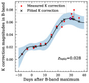
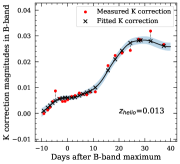
Figure 2: Examples of K-correction calculation for SN2016gcl (left) and SN2019vrq (right). The red data points are the K-correction values measured from mangled Hsiao’s template. The black line is the FPCA fit to the red data points. The shaded region is the error of the FPCA fit. And the black crosses are the adopted K-correction values derived from the fitted FPCA curve. By fitting a smooth curve to the measured K-correction, we can not only get the error estimates, but also the K-correction values of the epochs when colors are not available to which the spectra need to be mangled to match (one example is the purple diamond on the left panel).

To compare photometry of SNe at different redshifts, K-corrections are needed to account for the effect of the redshift on the observed magnitudes (Hamuy et al., 1993; Kim et al., 1996).

Before we calculate and apply the K-correction to the observed photometric light curves, the light curves are first corrected for extinction along the line-of-sight in the Milky Way (MW) using the MW dust map given by Schlegel et al. (1998), assuming the MW $R_{V}=3.1$ and a Fitzpatrick (1999) reddening law. Then the light curves are further corrected by removing the time dilation due to Hubble expansion. Corrected light curves are then fitted using the FPCA light curve fitting technique described above. The time of $B$-band maximum is then used to determine the rest-frame phase of the SN photometry to select the corresponding Hsiao et al. (2007) template spectrum to be used for K-corrections. In practice, the reddening is unknown before K-correction. The template is mangled using a smooth function to match the observed $B-V$ color when determining the $B$-band K-corrections, and $V-i^{\prime}/I/R$ when determining the $V$-band K-corrections to minimize extrapolation errors. The smooth function used to mangle the template spectra is the Fitzpatrick & Massa (1999) reddening law assuming $R_{V}=3.1$. The K-corrections are then measured by the difference in the synthetic magnitudes of the mangled spectrum at redshift of zero and the given redshift of the SN (shown as red data points in Figure 2). The filter-vague FPCA decomposition of He et al. (2018) shows that the light curves of SNe Ia can be decomposed into a single set of FPCA vectors independent of the filter bands employed. This implies that the K-correction itself can also be decomposed into the same FPCA basis. The measured K-correction magnitudes at different epochs are further fitted using the He et al. (2018) FPCA templates with the mean component taken out and the maximum epoch fixed by the previous FPCA fit using pycmpfit $\chi^{2}$ minimization. The final adopted values of the K-corrections (black cross in Figure 2) and their corresponding errors (shaded region in Figure 2) at desired epochs are then calculated from the fitted curve.

2.5 Host Reddening

Extinction can only make objects redder. Assuming that the intrinsic colors of SNe Ia are uniquely determined by the light curve width as measured by the $\Delta m_{15}(B)$ values, one can expect there to be a “blue edge” in the distribution of the observed colors when the observed colors are plotted together with the $\Delta m_{15}(B)$ (Fig. 3). With a large sample of SNe Ia, we may assume this blue edge to represent the intrinsic colors of SNe Ia for a given $\Delta m_{15}(B)$, and the reddening due to dust in the host galaxy $E(B-V)_{host}$ can be deduced by the difference between the observed colors and the this ridge line. Fig. 3 shows the MW- and K-corrected $B_{max}-V_{max}$ vs. $\Delta m_{15}(B)$. We estimate the position of the “blue edge” by fitting a second order polynomial ($B_{max}-V_{max}=A\times(\Delta m_{15}(B)-1.1)^{2}+C$ where A and C are parameters.) to the ridge line that divides the SN sample into two groups with the bluer group having 10 % of the total number of the SNe in the sample. To do so robustly, 500 bootstrapped samples are generated with replacement from the data set, leading to 500 estimates of the blue ridge lines. The median and standard deviation of these 500 ridge lines are used as the line of the intrinsic color and its corresponding uncertainties, respectively. Uncertainties of the host galaxy extinction are then estimated by the quadrature sum of uncertainties in $B_{max}-V_{max}$ and the uncertainties of the lower boundaries of the intrinsic colors. The equation for the final ridge line is

$$(B_{max}-V_{max})(mag)=0.188\times(\Delta m_{15}(B)(mag)-1.1)^{2}-0.021.$$

Figure 3: Observed $B_{max}-V_{max}$ (MW extinction and K-corrected) versus $\Delta m_{15}(B)$. Extinction can only cause $B_{max}-V_{max}$ to increase in value, thus the lower envelope (plotted as black solid line) can be used as an extinction free curve to correct for host extinction (subsection 2.5). 91T/99aa-like data points are plotted in green squares, and historical 91T/99aa-like data points are plotted in purple diamonds. Normal SNe Ia are plotted in grey triangles.

3 Spectra

Spectra of our 91T/99aa-like sample are plotted in Figure 9 at different epochs relative to the $B$ band maximum. For SN2018apo we do not have $B$-band photometry, so the maximum date was determined using $g$ band photometry. These spectra were collected from the Open Supernova Catalogue (Guillochon et al., 2017). The spectra are grouped into 5 groups each showing the data within 2 days of (a) $-$13 days, (b) $-$8 days, (c) $-$4 days, (d) 0 days, and (e) +6 days from $B$-band maximum for our 91T/99aa-like sample. The strength of the Si II $6355\pm 5\AA$ around maximum increases from top to bottom for each group. Spectra of SN1991T, SN1999aa, and the spectroscopically normal SN 2004eo at the relevant phases are plotted in bold lines together with each group for comparisons.

Not all 91T/99aa-like events classified by their spectra are slow decliners. The 91T/99aa-like objects with $\Delta m_{15}(B)>1.0$ mag are plotted in red in Figure 9. It is readily seen that some of the SNe with the shallowest Si II $\lambda\lambda$6355 lines are actually not slow decliners. The slowest decliners among 91T/99aa-like objects with $\Delta m_{15}(B)<0.8$ mag are plotted in dashed grey line. Although still showing shallower Si II lines, the spectra of 91T/99aa-like objects show all the major spectral features of normal SNe Ia at about 6 days after maximum. This suggests strongly that they share similar ejecta structures with spectroscopically normal SNe Ia and are likely originate from similar physical systems and processes.

3.1 Pseudo-equivalent widths

The true continuum in a SN Ia spectrum can not be formally determined, but the strength of an absorption line can be measured with respect to the flux at wavelengths shorter and longer than that of a given line. This is called the pseudo-equivalent width (pEW). It is defined as follows:

$$pEW\;=\;\sum_{i=1}^{N}\left(1-\frac{f(\lambda_{i})}{f_{c}(\lambda_{i})}\right)\;\;,$$ (4)

where $\lambda_{1}$ and $\lambda_{N}$ define the boundaries between which the pEW is calculated, $f(\lambda_{i})$ is the spectral flux at wavelength $\lambda_{i}$, and $f_{c}(\lambda_{i})$ is the pseudo continuum flux level defined by the line connecting the endpoints at $\lambda_{1}$ and $\lambda_{N}$.

To measure the pEW of the Si II $\lambda\lambda$6355 line, the endpoints are found by selecting the point with maximum flux of binned spectra (with a bin size of 40$\AA$) in the wavelength ranges [5820 $\AA$, 6000 $\AA$] and [6200 $\AA$, 6540 $\AA$] for the red side and blue side, respectively. The endpoints are further inspected by eye. We use a Monte Carlo method to calculate the errors of the pEW measurements. First we find the signal-to-noise ratio at each wavelength by dividing the original spectrum with a heavily smoothed spectrum (smoothed by the wavelet transformation method described by Wagers et al., 2010). Then the standard deviation of the signal-to-noise ratio at each pixel is found by the standard deviation of signal-to-noise ratios within 50 $\AA$. Next, we create a large number of simulated spectra with random noise generated using a Gaussian distribution with this calculated standard deviation. Finally, the pEW measurement is obtained for each of the simulated spectra, and the mean and the standard deviation of these pEW measurements give our final pEW value and its corresponding 1-$\sigma$ error.

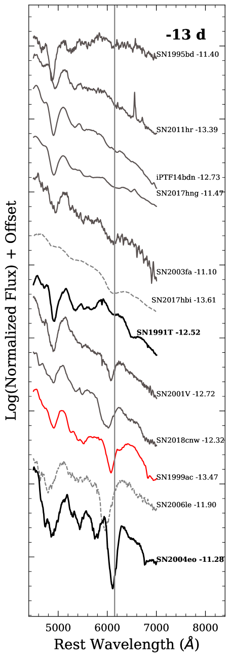
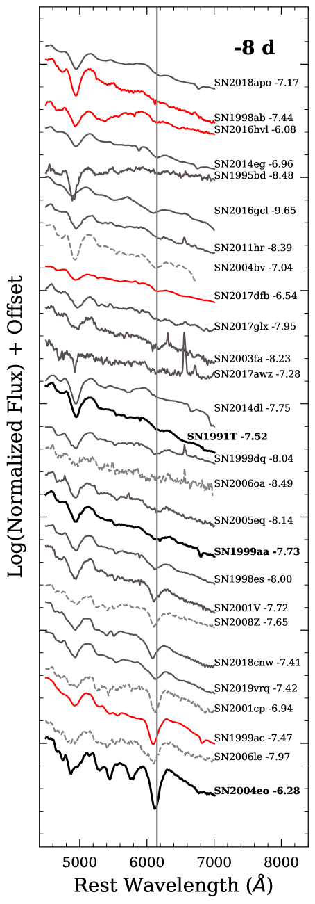
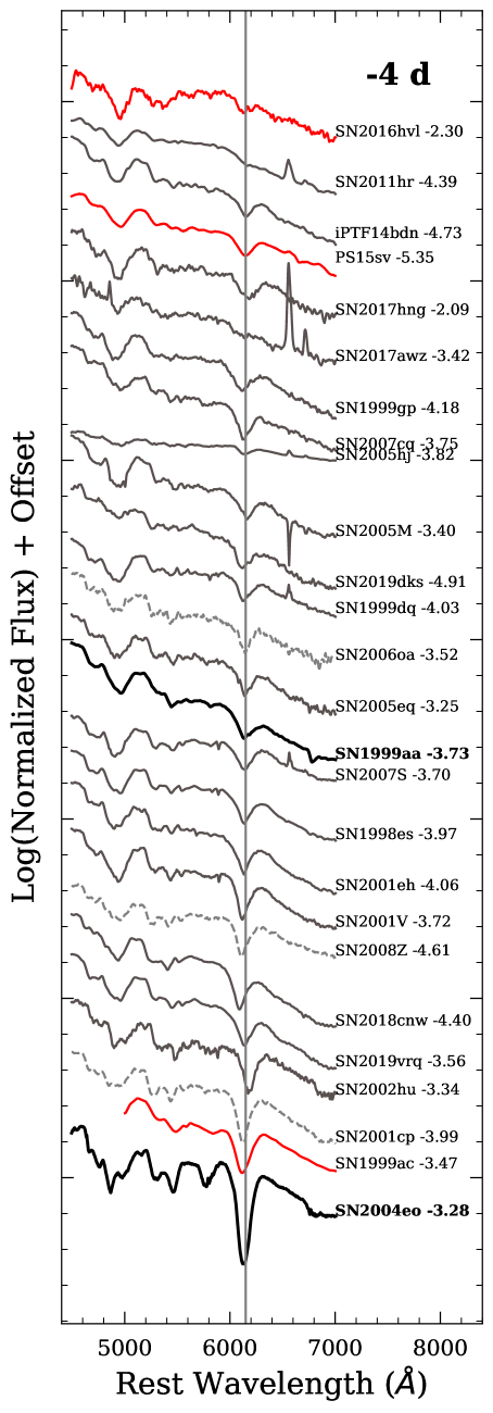
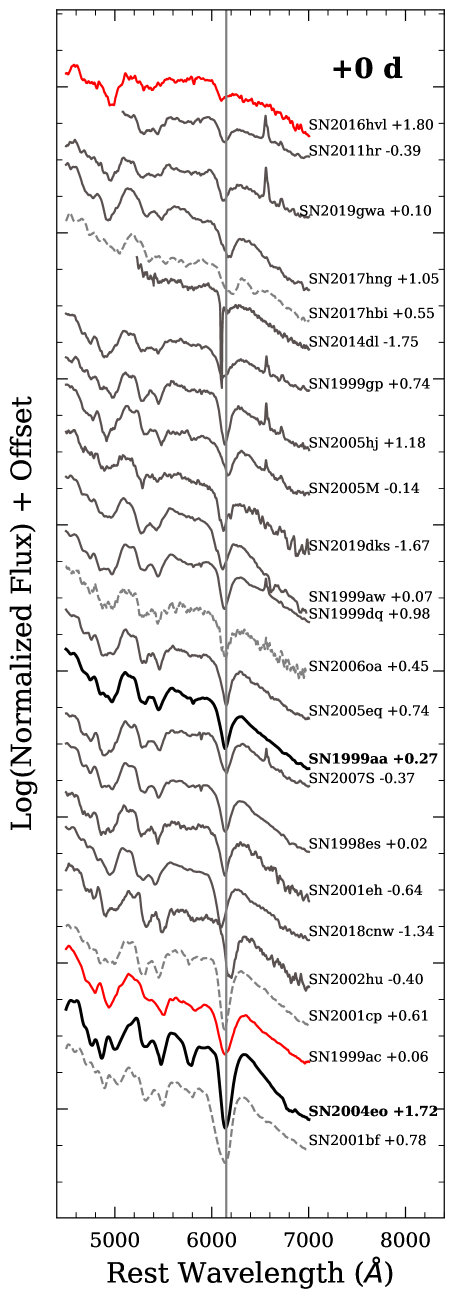
Figure 4: (a) Figure 5: (b) Figure 6: (c) Figure 7: (d) Figure 8: (e)

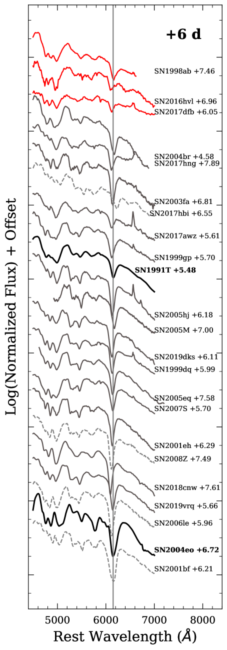
Figure 9: Spectra within 2 days of (a) $-$13 days; (b) $-$8 days; (c) $-$4 days; (d) 0 days; and (e) +6 days of our 91T/99aa-like sample. The Si II $6355\pm 5\AA$ around maximum increases from top to bottom for each panel. SN 1991T, SN 1999aa, and the typical normal Type Ia SN 2004eo are plotted in bold. 91T/99aa-like objects with $\Delta m_{15}(B)>1.0$ mag are plotted in red. And normal objects in our sample with $\Delta m_{15}(B)<0.8$ mag are also plotted in dashed grey lines. A vertical grey line at 6150 $\AA$ is also plotted to guide the eye.

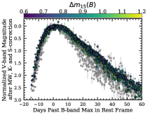
Figure 10: $B$- and $V$-band light curves for the SNe used in this paper. The light curves have been shifted vertically for better visualization. The grey data points are normal SNe Ia, while the data points of 91T/99aa-like SNe Ia are color coded by $\Delta m_{15}(B)$.

4 Standardization

The discovery of the accelerating expansion of the universe using SNe Ia was based on the discovery of the relationship between the SNe Ia peak luminosity magnitude and the light curve decline rate (Phillips, 1993) and the peak luminosity magnitude and color relationship found later (Hamuy et al., 1996c; Tripp, 1998), which make SNe Ia standardizable candles. 91T/99aa-like SNe Ia are inevitably over-represented in flux-limited surveys. Understanding the intrinsic properties of these SNe is therefore crucial to controlling the systematic errors when using SNe Ia to measure distances.

A Hubble diagram using SNe Ia can be used to constrain the cosmological acceleration parameters parameters, but it requires a high-redshift SNe Ia sample to be able to differentiate between different cosmology models (Goobar & Perlmutter, 1995). However, a nearby SNe Ia sample is also necessary to evaluate the precision of SNe Ia as standardizable candles, specifically, the standardizability of 91T/99aa-like objects in our case.

In this section, we evaluate the precision to which 91T/99aa-like SNe Ia may be used as standardizable candles. Recently, more sophisticated modeling and parameterization of SNe Ia are used for SNe Ia standardization, for example SALT2 (Guy et al., 2007, 2010; Betoule et al., 2014), SNEMO (Saunders et al., 2018), and SUGAR (Léget et al., 2020). Here we adopt the simple two-parameter parameterization using the decline rate $\Delta m_{15}(B)$ and host color excess $E(B-V)_{host}$ for standardization:

$$m_{B}^{*}\;=\;m_{B}(0)^{*}\;+\;b[\Delta m_{15}(B)-1.1]+R_{B}E(B-V)_{host}\;\;,$$ (5)

where $m_{B}^{*}=m_{B}-R_{B}E(B-V)_{gal}-K_{B}$ is the MW and K-corrected apparent peak magnitudes of SNe Ia in the $B$-band, $m_{B}(0)^{*}$ is the expected apparent peak magnitude of our fiducial SN Ia at redshift $z$, with $\Delta m_{15}(B)$ = 1.1 and $E(B-V)=0$. Here we adopt the approximation of $m_{B}(0)^{*}=5log_{10}(cz)+k$ as all SNe in our sample have $z\lesssim 0.1$. Thus, we immediately have $H_{0}=10^{0.2(M_{B}(0)+k+25)}$, where $M_{B}(0)$ is the absolute peak magnitude of a fiducial SN Ia. The global parameters are then ($b$, $R_{B}$, $k$) where $k$ is the intercept of the Hubble diagram. The Phillips luminosity-decline relationship (Phillips, 1993) is represented by the parameter $b$, the luminosity-color relationship is determined by $R_{B}$, and $k$ contains the information of Hubble constant at present, or equivalently, the absolute magnitude of the fiducial SN Ia.

In the analyses presented here, heliocentric redshifts were converted into the CMB frame using the velocity vector determined by Lineweaver (1997) to calculate luminosity distances. The uncertainty in the redshifts due to peculiar velocities is assumed to be $\sigma_{z}=0.001$ (300 km/s in velocity).

Parameters in Equation 5 are determined by fitting SNe in our sample with $z_{cmb}>0.01$ using $\chi^{2}$ minimization of

$$\chi^{2}=\sum_{i=1}^{N}\frac{(m_{Bcorr}^{*}-m_{B}(0)^{*})^{2}}{\sigma_{m_{Bcorr,i}^{*}}^{2}+\sigma_{intrinsic}^{2}+\sigma_{pec}^{2}}\;,$$ (6)

where $m_{Bcorr}^{*}=m_{B}^{*}-b\Delta(m_{15}(B)-1.1)-R_{B}E(B-V)$, $\sigma_{pec}$ accounts for peculiar velocity ($v_{pec}$ = 300 km s^-1),

$$\sigma_{m_{Bcorr}^{*}}^{2}=\sigma_{m_{B}^{*}}^{2}+b^{2}\sigma_{\Delta m_{15}(B)}^{2}+R_{B}^{2}\sigma_{E(B-V)}^{2}\;,$$ (7)

and $\sigma_{intrinsic}^{2}$ accounts for possible intrinsic scatter in SNe Ia, which is determined so that the final $\chi^{2}_{\nu}=1$.

Table 7: Parameters of 91T/99aa-like SNe Ia in our sample.

SN (subtype)	$z_{CMB}$	$pEW_{nearmax}(\text{Si II }\lambda 6355)$	$E(B-V)_{host}$	Hubble Residual	$t_{max}(B)$	$\Delta m_{15}(B)$	$m_{max}(B)$	SN (subtype)	PC1(B)	PC2(B)	$t_{max}(V)$	$\Delta m_{15}(V)$	$m_{max}(V)$	PC1(V)	PC2(V)
		($\AA$)		(mag)	(MJD)	(mag)	(mag)				(MJD)	(mag)	(mag)
LSQ15aae	0.0518	…	0.27 (0.04)	-0.35 (0.31)	57116.45 (0.35)	0.88 (0.05)	17.77 (0.03)		-0.28 (0.32)	-0.03 (0.20)	57118.78 (0.35)	0.58 (0.04)	17.51 (0.02)	-0.39 (0.24)	0.00 (0.12)
PS15sv (3)	0.0333	32.0	0.05 (0.04)	-0.26 (0.33)	57114.35 (0.85)	1.07 (0.05)	16.31 (0.04)		1.25 (0.51)	-0.35 (0.21)	57115.85 (0.32)	0.69 (0.03)	16.28 (0.02)	0.52 (0.19)	0.04 (0.08)
SN1991T (4)	0.0069	42.2	0.21 (0.02)	-2.00 (0.47)	48375.52 (0.18)	0.94 (0.01)	11.60 (0.01)		-0.13 (0.09)	-0.06 (0.04)	48378.19 (0.12)	0.62 (0.01)	11.41 (0.01)	-0.34 (0.07)	0.19 (0.04)
SN1995bd (2)	0.0144	20.1	0.44 (0.04)	-0.38 (0.35)	50085.74 (0.21)	0.85 (0.05)	15.51 (0.03)		-0.98 (0.31)	0.24 (0.13)	50087.50 (0.22)	0.69 (0.04)	15.08 (0.02)	-0.29 (0.23)	0.43 (0.11)
SN1998ab (0)	0.0279	4.5	0.10 (0.05)	-0.37 (0.34)	50913.82 (0.16)	1.09 (0.04)	16.00 (0.03)		1.48 (0.28)	-0.46 (0.09)	50915.94 (0.25)	0.62 (0.04)	15.92 (0.03)	0.12 (0.25)	-0.10 (0.11)
SN1998es (5)	0.0096	53.0	0.14 (0.01)	-0.01 (0.35)	51142.20 (0.04)	0.71 (0.01)	13.87 (0.01)		-0.78 (0.08)	-0.67 (0.04)	51144.30 (0.05)	0.52 (0.01)	13.72 (0.01)	-0.76 (0.05)	-0.10 (0.03)
SN1999aa (5)	0.0152	52.4	0.01 (0.01)	0.29 (0.32)	51231.73 (0.04)	0.73 (0.01)	14.76 (0.01)		-0.55 (0.05)	-0.74 (0.03)	51233.92 (0.05)	0.54 (0.01)	14.74 (0.00)	-0.51 (0.04)	-0.12 (0.02)
SN1999ac (8)	0.0098	80.4	0.06 (0.02)	0.01 (0.37)	51249.47 (0.03)	1.20 (0.01)	14.07 (0.01)		1.09 (0.05)	0.20 (0.03)	51252.63 (0.07)	0.65 (0.01)	14.03 (0.00)	0.41 (0.04)	-0.12 (0.03)
SN1999aw (4)	0.0392	48.7	0.12 (0.02)	-0.11 (0.29)	51253.93 (0.23)	0.68 (0.01)	16.72 (0.01)		-1.90 (0.11)	0.15 (0.04)	51255.63 (0.24)	0.57 (0.02)	16.59 (0.01)	-1.27 (0.10)	0.45 (0.07)

Table 8: Parameters of normal SNe Ia in our sample.

SN (subtype)	$z_{CMB}$	$pEW_{nearmax}(\text{Si II }\lambda 6355)$	$E(B-V)_{host}$	Hubble Residual	$t_{max}(B)$	$\Delta m_{15}(B)$	$m_{max}(B)$	SN (subtype)	PC1(B)	PC2(B)	$t_{max}(V)$	$\Delta m_{15}(V)$	$m_{max}(V)$	PC1(V)	PC2(V)
		($\AA$)		(mag)	(MJD)	(mag)	(mag)				(MJD)	(mag)	(mag)
SN1998dh (C)	0.0078	121.6	0.12 (0.02)	0.09 (0.25)	51029.19 (0.03)	1.23 (0.01)	13.88 (0.00)		2.01 (0.05)	-0.40 (0.03)	51031.57 (0.04)	0.69 (0.01)	13.77 (0.01)	0.90 (0.04)	-0.25 (0.02)
SN1998dm (6)	0.0060	68.4	0.33 (0.02)	1.07 (0.32)	51060.38 (0.07)	0.87 (0.01)	14.68 (0.01)		0.14 (0.10)	-0.61 (0.04)	51062.06 (0.05)	0.60 (0.01)	14.37 (0.01)	-0.08 (0.06)	-0.07 (0.02)
SN1999cp (9)	0.0099	99.6	0.04 (0.02)	0.10 (0.25)	51363.46 (0.04)	0.99 (0.01)	13.93 (0.00)		0.90 (0.06)	-0.60 (0.04)	51364.71 (0.05)	0.66 (0.01)	13.91 (0.00)	0.15 (0.05)	0.09 (0.03)
SN1999dk (C)	0.0140	126.4	0.12 (0.02)	-0.15 (0.18)	51414.78 (0.13)	1.09 (0.02)	14.79 (0.01)		1.48 (0.16)	-0.54 (0.09)	51416.88 (0.15)	0.68 (0.02)	14.69 (0.01)	0.63 (0.13)	-0.13 (0.06)
SN2000cn (B)	0.0227	118.6	0.17 (0.02)	-0.05 (0.12)	51707.17 (0.04)	1.63 (0.02)	16.53 (0.01)		4.78 (0.23)	-0.62 (0.15)	51709.58 (0.08)	0.96 (0.01)	16.33 (0.01)	3.79 (0.22)	-0.61 (0.11)
SN2000cw (B)	0.0288	111.4	0.11 (0.02)	0.11 (0.12)	51748.18 (0.19)	1.18 (0.03)	16.66 (0.01)		2.31 (0.46)	-0.64 (0.34)	51751.05 (0.22)	0.69 (0.02)	16.57 (0.01)	1.23 (0.34)	-0.45 (0.19)
SN2000dk (C)	0.0160	121.6	-0.01 (0.02)	0.05 (0.15)	51812.27 (0.06)	1.64 (0.02)	15.30 (0.01)		4.29 (0.15)	-0.22 (0.09)	51814.42 (0.06)	0.95 (0.01)	15.28 (0.01)	3.33 (0.09)	-0.44 (0.06)
SN2000dn (9)	0.0307	98.7	0.08 (0.04)	0.06 (0.15)	51824.74 (0.14)	1.06 (0.04)	16.55 (0.02)		1.32 (0.36)	-0.47 (0.25)	51827.22 (0.17)	0.69 (0.03)	16.49 (0.02)	0.94 (0.24)	-0.23 (0.14)
SN2000dr (C)	0.0180	124.9	0.08 (0.03)	-0.04 (0.16)	51834.31 (0.09)	1.84 (0.03)	15.94 (0.01)		5.00 (0.00)	0.27 (0.16)	51836.42 (0.14)	1.00 (0.02)	15.77 (0.01)	3.52 (0.19)	-0.32 (0.12)
SN2000fa (9)	0.0215	90.9	0.19 (0.02)	-0.05 (0.13)	51891.96 (0.14)	0.89 (0.02)	15.91 (0.01)		0.30 (0.13)	-0.59 (0.07)	51893.77 (0.22)	0.60 (0.01)	15.73 (0.01)	-0.03 (0.09)	-0.13 (0.05)

5 Results

5.1 Photometric properties of 91T/99aa-like SNe Ia

The $B$- and $V$-band light curves of the SNe used in this analysis are plotted together in Figure 10. Gray points are for normal SNe Ia while 91T/99aa-like objects are color coded by the value of $\Delta m_{15}(B)$. As expected, light curves of 91T/99aa-like SNe are typically broader compared to normal SNe Ia. This trend is more pronounced in the $V$-band.

Host galaxy extinction needs to be taken out if one wants to compare the intrinsic brightness of 91T/99aa-like SNe to normal SNe Ia. The extinction is commonly characterized by the total-to-selective extinction ratio $R_{V}=A_{V}/E(B-V)$, where $E(B-V)=A_{B}-A_{V}$. Previous studies of the host extinction from SNe Ia yielded diverse values of $R_{V}$ ranging from $R_{V}=1$ to $R_{V}=3.5$ (e.g. Tripp, 1998; Phillips et al., 1999; Conley et al., 2007; Hicken et al., 2009; Wang et al., 2009). For a rough comparison of the intrinsic luminosity distributions between 91T/99aa-like SNe and normal SNe Ia without any standardization, we take a moderate value of $R_{V(host)}=2$ with $E(B-V)_{host}$ calculated from subsection 2.5. In Figure 11 we plot the distribution of the decline rate parameter $\Delta m_{15}(B)$, and the extinction- and K-corrected absolute $B-$band magnitudes when assuming host $R_{V}=2$ for all 123 SNe Ia included in this work (SN2018apo is not included in this figure as we do not have SN2018apo B-band data.). The distance moduli are calculated using aforementioned assumed cosmology. The weighted mean and standard deviation of the full sample’s absolute peak $B$-band magnitude and $\Delta m_{15}(B)$ are listed in Table 9.

The spectroscopically peculiar 91T/99aa-like objects are $\sim$ 0.4 mag brighter than normal SNe Ia after applying K-corrections and correcting for Milky Way extinction and host galaxy extinction. Moreover, these overluminous events seem to have a more uniform peak luminosity and a more uniform distribution of values of the decline rate parameter $\Delta m_{15}(B)$, with a standard deviation of about 0.13 mag compared to 0.32 mag for normal SN Ia.

Table 9: Weighted means and standard deviations of absolute peak magnitudes and $\Delta m_{15}(B)$ in Figure 11.

SN subclass	$N_{SN}$	$\overline{M_{B}}$	$\sigma_{M_{B}}$	$\overline{\Delta m_{15}(B)}$	$\sigma_{\Delta m_{15}(B)}$
Normal	87	-19.30	0.47	1.09	0.32
91T/99aa-like	36	-19.70	0.32	0.82	0.13

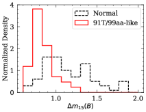
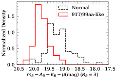
Figure 11: Left: Histogram of $\Delta m_{15}$ in $B$ band. Right: Histogram of absolute magnitudes at maximum in $B$ band assuming a constant $R_{B}=3$.

5.2 The Hubble diagram

We standardize our sample using the method described in section 4 in two cases: for one we assume 91T/99aa-like and normal SNe Ia share the same intrinsic scatter $\sigma_{int}$, and for the other we assume each group has a different intrinsic scatters $\sigma_{int}(\text{91T/99aa-like})$ and $\sigma_{int}(\text{normal})$ (so that for each group, $\chi^{2}_{\nu}\approx 1$ after fitting). Final fitting parameters for both cases are summarized in Table 10. And the Hubble residuals for the case with different intrinsic scatters are listed in Table 7 and Table 8. Below we focus on the case with different intrinsic scatters.

In Figure 12, we present the $B$ band residual Hubble diagram, and the histogram of Hubble residuals along with the fitted Gaussian ideogram . The weighted mean Hubble residual for normal SNe Ia and 91T/99aa-like SNe Ia with $z_{cmb}>0.01$ are 0.03 mag and -0.19 mag respectively, and the peak in Gaussian ideogram for normal SNe Ia and all 91T/99aa-like SNe Ia in our sample are 0.01 mag and -0.17 mag respectively, suggesting that even fully corrected, 91T/99aa-like SNe Ia still are $\sim 0.2$ mag brighter than normal SNe Ia (Reindl et al., 2005; Boone et al., 2021). Therefore careful classification of 91T/99aa-like SNe is needed to avoid possible pollution to the cosmological sample of SNe Ia, or to introduce an additional parameter to account for the Hubble residual offset in 91T/99aa-like and normal SNe.

The intrinsic scatter for 91T/99aa-like is $\sigma_{int}\text{(91T/99aa-like)}=0.28$ mag, more than that of normal SNe Ia ($\sigma_{int}\text{(normal)}=0.05$ mag). The weighted root mean square (wRMS) are $0.25\pm 0.03$ mag and $0.14\pm 0.02$ mag for 91T/99aa-like and normal SNe Ia respectively. It suggests that 91T/99aa-like SNe are also excellent relative distance indicators, though not as precise as normal SNe Ia, and can be used to delineate the Hubble flow to a precision of 12%. However, an additional parameter needs to be introduced to bring 91T/99aa-like SNe to the same standard value as normal SNe Ia. Note that for absolute distance determination, it requires independent estimates of nearby SN hosts (e.g. Riess et al., 2019), which is beyond the scope of this paper.

Table 10: Fitting parameters of Hubble diagram.

Condition on $\sigma_{int}$	b	$R_{B}$	k	$\sigma_{int}$		RMS ($z_{cmb}>0.01$)		wRMS ($z_{cmb}>0.01$)
				(mag)		(mag)		(mag)
				normal	91T/99aa-like	normal	91T/99aa-like	normal	91T/99aa-like
$\sigma_{int(normal)}=\sigma_{int(91T/99aa)}$	$0.88\pm 0.06$	$3.13\pm 0.17$	$-3.58\pm 0.03$	0.14	0.14	$0.18\pm 0.03$	$0.25\pm 0.03$	$0.16\pm 0.02$	$0.24\pm 0.03$
$\sigma_{int(normal)}\neq\sigma_{int(91T/99aa)}$	$0.81\pm 0.05$	$3.35\pm 0.15$	$-3.57\pm 0.02$	0.05	0.28	$0.17\pm 0.02$	$0.26\pm 0.03$	$0.14\pm 0.02$	$0.25\pm 0.03$

Note. — comments

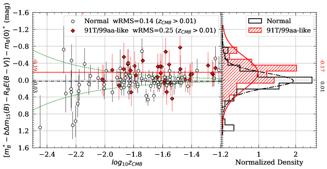
Figure 12: Hubble Diagram Residual (left) and residual histogram (right) in B band for 36 91T/99aa-like SNe Ia (in filled circles) and 87 normal SNe Ia (in open circles) when assuming these two groups have different intrinsic scatters (0.28 mag for 91T/99aa-like, and 0.05 mag for normal Iae). Left: The weighted mean Hubble residuals for 91T-like SNe Ia and normal SNe Ia are 0.03 mag and -0.18 mag, which are also plotted as horizontal lines on the plot (solid line for 91T-like SNe, dash dotted line for normal SNe Ia). Dashed line denotes the peculiar velocity effect with $v_{pec}=300km/s$. Right: Distribution of Hubble residuals. Gaussian ideograms of each group are also plotted (solid line for 91T/99aa-like, dash dotted line for normal SNe Ia). The peak of resulting Gaussian ideograms are 0.01 mag and -0.17 mag for normal SNe Ia and 91T/99aa-like SNe Ia respectively.

5.3 Si II $\lambda\lambda$6355 pEW

We used pEW measurements of the Si II $\lambda\lambda$6355 line from the spectra in our database that are closest to—and within 10 days from—$B$ band maximum as our Si II $\lambda\lambda$6355 pEW measurement around maximum. In total, we have such measurements of 79 normal SNe Ia and 35 91T/99aa-like SNe. Final pEW measurements are listed in Table 7 and Table 8. Hubble residuals versus $pEW_{max}$(Si II $\lambda\lambda$6355)are plotted in Figure 15.(See also M. M. Phillips 2023 for further discussion). As $pEW_{max}$(Si II $\lambda\lambda$6355) increases from 0 Å to 150 Å, Hubble residuals increase first and then stay nearly constant. Thus we fit a continuous broken line so that Hubble residual linearly increases with $pEW_{max}$(Si II $\lambda\lambda$6355) first, and stays constant beyond a $pEW_{max}$(Si II $\lambda\lambda$6355) value. The line is fitted using $\chi^{2}$ minimization (See section 15.3 in Press et al., 2007) with pycmpfit. The best fitted result is

$$\text{Hubble Residual (mag)}=\begin{cases}(0.009\pm 0.003)\times\text{ pEW}(\text{Si II }\lambda\lambda 6355)(\AA)-(0.482\pm 0.154),&\text{ pEW}(\text{Si II }\lambda\lambda 6355)<55.62\AA\\ 0.036,&\text{Otherwise.}\par\end{cases}$$ (8)

There does not seem to be a correlation between the Hubble residual and $\Delta m_{15}(B)$ as shown in the left panel in Figure 14. Thus the broken linear correlation between the Hubble residual and Si II $\lambda\lambda$6355 is unlikely due to the artifacts of standardizations. As shown in the right panel of Figure 14, the relation between $\Delta m_{15}(B)$ and $pEW_{max}$(Si II $\lambda\lambda$6355) is non-linear. Thus a linear correlation of $\Delta m_{15}(B)$ to Hubble residual cannot fully take out the dependency of Hubble residual on $pEW_{max}$(Si II $\lambda\lambda$6355).

For our sample of 113 objects with $\text{pEW}(\text{Si II }\lambda\lambda 6355)$ near maximum and B-band light curve data, after taking out the fitted linear relationship between $pEW_{max}$(Si II $\lambda\lambda$6355) and light curve shape- and color- corrected Hubble residual, the wRMS of the Hubble residuals of the 113 objects decreases from 0.17 mag to 0.14 mag (for 34 91T/99aa-like objects, wRMS decreases from 0.26 mag to 0.22 mag, and for 79 normal objects, wRMS decreases from 0.129 mag to 0.125 mag).

The Hubble residual offset in 91T/99aa-like and normal SNe Ia can then be explained by the positive linear correlation in between the Hubble residual and the pEW, as most SNe Ia have $pEW_{max}$(Si II $\lambda\lambda$6355)$<55.6\AA$, and 91T/99aa-like SNe are characterized by the shallow Si II lines.

We suggest a new sub-type classification scheme amongst SNe Ia as follows. The SNe Ia is subdivided using a hexadecimal number with 0 being the extreme SN1991T-like showing undetectable Si II $\lambda\lambda$6355 line, and F being the extreme case with the $pEW_{max}$(Si II $\lambda\lambda$6355) beyond 160 Å. In between these extreme cases, the sub-types are given by a hexadecimal number that is the integer part of $pEW_{max}$(Si II $\lambda\lambda$6355)/10. The sub-types of SNe in our sample are given in Table 7 and Table 8.

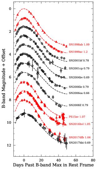
Figure 13: B-band light curves and fits of normal SNe Ia (in black circles) with $\Delta m_{15}(B)<0.8$ mag and 91T/99aa-like SNe (in red triangles) with $\Delta m_{15}(B)>1.0$ mag. $\Delta m_{15}(B)$ values are labeled next to each light curve.

In the right panel of Figure 14 we plot the $pEW_{max}$(Si II $\lambda\lambda$6355) vs $\Delta m_{15}(B)$. As can be seen from the figure, $\Delta m_{15}(B)$ does not always increase as $pEW_{max}$(Si II $\lambda\lambda$6355) increases. There are a few objects with normal decline rate yet have very shallow Si II lines, and objects with slow decline rate but moderate strength of Si II lines. To show that the effect is not some artifacts from fitting, the light curves of normal objects with $\Delta m_{15}(B)<0.8$ mag and 91T/99aa-like objects with $\Delta m_{15}(B)>1.0$ mag are shown in Figure 13, and their spectra are highlighted in Figure 9.

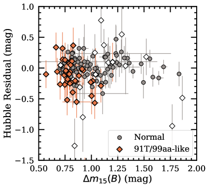
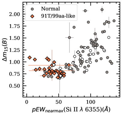
Figure 14: Left: Hubble residual vs. $\Delta m_{15}(B)$. Right: $\Delta m_{15}(B)$ vs. $pEW_{max}$(Si II $\lambda\lambda$6355).

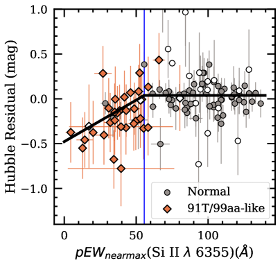
Figure 15: Hubble residual vs. $pEW_{max}$(Si II $\lambda\lambda$6355). Open circles indicate objects with $z_{cmb}<0.01$. Blue vertical line is where pEW=55.62$\AA$. Black line shows the best linear fit for objects with pEW $<$ 55.62 $\AA$ (Hubble residual (mag) = $0.009\times pEW_{max}\text{Si II}\lambda 6355(\AA)-0.482$), and the weighted mean (=0.036 mag) for objects with pEW $>$ 55.62 $\AA$.

6 Discussion and Conclusions

Spectroscopically confirmed peculiar SNe Ia such as overluminous 91T/99aa-like SNe Ia have generally been excluded from cosmological use of SNe Ia. However, those overluminous events will be over-represented in future flux-limited surveys. Furthermore, the spectral evolution of 91T/99aa-like objects resembles that of normal SNe Ia after maximum light, which makes keeping the homogeneity of the SNe Ia cosmological sample more difficult. Hence, it is crucial to understand the intrinsic properties of these over-luminous SNe Ia to avoid inevitable systematic errors in luminosity distances.

To address this problem, We obtained multi-epoch optical $BVg^{\prime}r^{\prime}i^{\prime}$ photometric observations of 16 91T/99aa-like SNe Ia taken by Las Cumbres Observatory in the redshift range $z=0.011-0.057$. This sample was analyzed together with 21 well sampled photometric observations of 91T/99aa-like SNe Ia as well as 87 photometrically well sampled normal SNe Ia from the literature. Our main conclusions are as follows:

1. When assuming host $R_{V}=2$, after correcting for K-correction, MW extinction and host extinction, the spectroscopically peculiar 91T/99aa-like objects are $\sim$0.4 mag brighter than the normal SNe Ia.

2. After fully corrected (see section 4), 91T/99aa-like objects are still $\sim$0.2 mag brighter than normal SNe Ia.

3. 91T/99aa-like objects themselves are excellent relative distance indicators and can be used to delineate galaxies in the Hubble flow to 12% in distance.

4. $\Delta m_{15}(B)$ does not always increases as $pEW_{max}$(Si II $\lambda\lambda$6355) increases. For $pEW_{max}$(Si II $\lambda\lambda$6355)$<55.6\AA$, light curves tend to decline faster with shallower Si II $\lambda\lambda$6355 .

5. After fully corrected, the Hubble residual still has a fairly strong linear correlation with $pEW_{max}$(Si II $\lambda\lambda$6355) for $pEW_{max}$(Si II $\lambda\lambda$6355)$<55.6\AA$ while the Hubble residual does not correlate with $\Delta m_{15}(B)$. This is due to the non-linear relation between $\Delta m_{15}(B)$ and $pEW_{max}$(Si II $\lambda\lambda$6355). So a linear correction of $\Delta m_{15}(B)$ cannot fully take out the dependence of the Hubble residual on $pEW_{max}$(Si II $\lambda\lambda$6355) if any.

The current study is based on the optical data. In the NIR, the systematic offset of the Hubble residuals between 91T/99aa-like and normal SNe may be different from the optical. A careful analyses for the NIR properties of 91T/99aa-like SNe is needed.

The spectral evolution of 91T/99aa-like SNe Ia argues that early spectral data are needed for their identification. This may cause the SN Ia samples to be contaminated by mis-identifications of 91T/99aa-like SNe if spectral data before optical maximum are missing. This would lead to large systematic biases in cosmological analyses if the fraction of 91T/99aa-like SNe Ia changes with redshift. High-mass but passive hosts are observed to produce SNe Ia over the full range of decline rates, whereas low-mass, star-forming hosts (which increase with redshift Noeske et al., 2007; Daddi et al., 2007; Elbaz et al., 2007) preferentially give rise to slower declining events like 91T/99aa-like SNe (Sullivan et al., 2010; Uddin et al., 2020). The fractional evolution of 91T/99aa-like SNe Ia will cause systematic errors of the SNe Ia Hubble residual to be as large as 0.2 mag in the extreme case at high redshifts where SNe Ia are dominated by 91T/99aa-like events. This will be very important on upcoming surveys like LSST/Rubin and WFIRST/Roman for which the projected uncertainties are smaller than the effects reported here.

Based on the post-maximum spectral similarities between 91T/99aa-like SNe Ia and the normal SNe Ia, it may be concluded that the 91T/99aa-like SNe Ia and normal SNe Ia could easily be confused with just photometric data. It is critical to identify them in future supernova surveys which aim at much higher precision than today in cosmological applications. The 0.2 mag correction between 91T/99aa-like SNe and normal SNe Ia also depends on the relative abundances of 91T/99aa-like objects at different $pEW_{max}$(Si II $\lambda\lambda$6355) since 91T/99aa-like objects with lower $pEW_{max}$(Si II $\lambda\lambda$6355) have brighter Hubble residuals. Therefore it will be necessary to construct a classification scheme of the 91T/99aa-like SNe. The correlation between the Hubble residual and pEW of Si II $\lambda\lambda$6355 line seen in Figure 15 suggests that the strength of the Si II $\lambda\lambda$6355 line can be employed to sub-classify SNe Ia. Instead of classifying SNe Ia with descriptive monikers such as 91T/99aa-like or shallow silicon, we suggest dividing the SNe Ia Types into sub-classes based on the values of $pEW_{max}$(Si II $\lambda\lambda$6355). The measured pEW values are typically in the range from 0 to 160 (see Figure 15); A single hexadecimal digit can be used to group them in intervals of 10, with the last class being inclusive of all SNe with $pEW_{max}$(Si II $\lambda\lambda$6355) larger than 160 Å. The sub-classification is natural as the presence of Si II is the basis for SN Ia classification. As the Si II line changes rapidly around maximum light, in the case where it is not easy to obtain spectra around maximum light, we recommend using the data-driven spectral modelling code introduced in Hu et al. (2022a), which is able to model the spectrum at maximum well given observed spectra at other phases.

Another systematic effect that is routinely addressed recently in cosmological sample is a $\sim$ 0.06 mag correction found from the empirical correlation in between SN Ia corrected Hubble residuals with host galaxy mass (the mass step; Kelly et al., 2010; Sullivan et al., 2010; Lampeitl et al., 2010; Gupta et al., 2011; Childress et al., 2013; Johansson et al., 2013). SNe Ia in high-mass, passive hosts appear to be brighter than those in low mass, star-forming hosts. It can be easily seen that 91T/99aa-like SNe Ia have a host mass step that is in the opposite direction since they are associated with active star formation (Hakobyan et al., 2020). Thus the fraction of 91T/99aa-like SNe Ia will affect the size of the mass step. These effects need to be carefully taken into account for future surveys to measure cosmological parameters with better control of systematics for future surveys. Our study suggests further that the shallow Si II line SNe Ia cannot be the source of the mass step effect, and that the mass step is caused by the SNe Ia with normal Si II line strength. However, for SNe at high redshifts, the fractional contribution of 91T/99aa-like events may become larger which will lead to a systematic effect that must be taken into account for precision cosmology measurements.

The correlation between luminosity and the pEW of the Si II 6355 line may also suggest that the group of 91T/99aa-like events consists of SNe with related physical origins. One such possibility is that they are similar events that differ in such effects as arising from geometric orientations and subtle physical processes at the explosion. The SNe with more complete nuclear burning which converts Si to Fe group elements show shallower Si II lines (see Figure 14, right panel). At the luminous end, with $\Delta m_{15}\lesssim 1$, the light curve shape is insensitive to these effects but the luminosity is correlated with the strength of the Si II 6355 line (see Figure 15). In the context of delayed detonation, this may be further related to the central density at ignition and the mass of the progenitors (Khokhlov, 1991; Khokhlov et al., 1993; Höflich et al., 1996; Hoeflich et al., 2017). Quantitative modeling of these physical processes is beyond the scope of this study. If geometric effect dominates the observed luminosity and Si II 6355 line strength correlation, Figure 15 suggests that the side with more advanced nuclear burning shows weaker Si II lines when faced with the observer. The geometry of SNe Ia has been probed by spectropolarimetry, and the degree of continuum polarization is consistently low ($\lesssim 0.2\%$). The level of Si II 6355 line polarization is around 0.5% in general (Wang & Wheeler, 2008; Cikota et al., 2019; Yang et al., 2020). There have been no published spectropolarimetry data that can place tight constraints on the geometric shapes of the 91T/99aa-like events, although recent data seem to indicate that they are very lowly polarized similar to other SNe Ia (Y. Yang, private communications). If geometric effect does play a role, spectroscopy during the late time nebular phase can also be of great diagnostic value. Interestingly, these observations are qualitatively consistent with the discovery that the SNe with larger light curve stretch values are both more luminous and less polarized (Wang et al., 2007; Cikota et al., 2019). The more complete burning effectively removes the asymmetries arising from the instabilities during the deflagration phase preceding the detonation.

References

- Altavilla et al. (2004) Altavilla, G., Fiorentino, G., Marconi, M., et al. 2004, MNRAS, 349, 1344, doi: 10.1111/j.1365-2966.2004.07616.x
- Baltay et al. (2021) Baltay, C., Grossman, L., Howard, R., et al. 2021, Publications of the Astronomical Society of the Pacific, 133, 44002, doi: 10.1088/1538-3873/abd417
- Benetti et al. (2005) Benetti, S., Cappellaro, E., Mazzali, P. A., et al. 2005, ApJ, 623, 1011, doi: 10.1086/428608
- Bertin et al. (2002) Bertin, E., Mellier, Y., Radovich, M., et al. 2002, in Astronomical Society of the Pacific Conference Series, Vol. 281, Astronomical Data Analysis Software and Systems XI, ed. D. A. Bohlender, D. Durand, & T. H. Handley, 228
- Bessell (1990) Bessell, M. S. 1990, PASP, 102, 1181, doi: 10.1086/132749
- Betoule et al. (2014) Betoule, M., Kessler, R., Guy, J., et al. 2014, A&A, 568, A22, doi: 10.1051/0004-6361/201423413
- Blondin et al. (2012) Blondin, S., Matheson, T., Kirshner, R. P., et al. 2012, AJ, 143, 126, doi: 10.1088/0004-6256/143/5/126
- Boone et al. (2021) Boone, K., Aldering, G., Antilogus, P., et al. 2021, ApJ, 912, 71, doi: 10.3847/1538-4357/abec3b
- Branch et al. (2006) Branch, D., Dang, L. C., Hall, N., et al. 2006, PASP, 118, 560, doi: 10.1086/502778
- Brown et al. (2014) Brown, P. J., Breeveld, A. A., Holland, S., Kuin, P., & Pritchard, T. 2014, Ap&SS, 354, 89, doi: 10.1007/s10509-014-2059-8
- Brown et al. (2013) Brown, T. M., Baliber, N., Bianco, F. B., et al. 2013, PASP, 125, 1031, doi: 10.1086/673168
- Burns et al. (2011) Burns, C. R., Stritzinger, M., Phillips, M. M., et al. 2011, AJ, 141, 19, doi: 10.1088/0004-6256/141/1/19
- Burrow et al. (2020) Burrow, A., Baron, E., Ashall, C., et al. 2020, ApJ, 901, 154, doi: 10.3847/1538-4357/abafa2
- Childress et al. (2013) Childress, M., Aldering, G., Antilogus, P., et al. 2013, ApJ, 770, 108, doi: 10.1088/0004-637X/770/2/108
- Cikota et al. (2019) Cikota, A., Patat, F., Wang, L., et al. 2019, MNRAS, 490, 578, doi: 10.1093/mnras/stz2322
- Conley et al. (2007) Conley, A., Carlberg, R. G., Guy, J., et al. 2007, ApJL, 664, L13, doi: 10.1086/520625
- Daddi et al. (2007) Daddi, E., Dickinson, M., Morrison, G., et al. 2007, ApJ, 670, 156, doi: 10.1086/521818
- DePoy et al. (2003) DePoy, D. L., Atwood, B., Belville, S. R., et al. 2003, in Society of Photo-Optical Instrumentation Engineers (SPIE) Conference Series, Vol. 4841, Instrument Design and Performance for Optical/Infrared Ground-based Telescopes, ed. M. Iye & A. F. M. Moorwood, 827–838, doi: 10.1117/12.459907
- Elbaz et al. (2007) Elbaz, D., Daddi, E., Le Borgne, D., et al. 2007, A&A, 468, 33, doi: 10.1051/0004-6361:20077525
- Filippenko et al. (1992a) Filippenko, A. V., Richmond, M. W., Matheson, T., et al. 1992a, ApJL, 384, L15, doi: 10.1086/186252
- Filippenko et al. (1992b) Filippenko, A. V., Richmond, M. W., Branch, D., et al. 1992b, AJ, 104, 1543, doi: 10.1086/116339
- Fitzpatrick (1999) Fitzpatrick, E. L. 1999, PASP, 111, 63, doi: 10.1086/316293
- Fitzpatrick & Massa (1999) Fitzpatrick, E. L., & Massa, D. 1999, ApJ, 525, 1011, doi: 10.1086/307944
- Foley et al. (2018) Foley, R. J., Scolnic, D., Rest, A., et al. 2018, MNRAS, 475, 193, doi: 10.1093/mnras/stx3136
- Freedman et al. (2001) Freedman, W. L., Madore, B. F., Gibson, B. K., et al. 2001, ApJ, 553, 47, doi: 10.1086/320638
- Fukugita et al. (1996) Fukugita, M., Ichikawa, T., Gunn, J. E., et al. 1996, AJ, 111, 1748, doi: 10.1086/117915
- Ganeshalingam et al. (2010) Ganeshalingam, M., Li, W., Filippenko, A. V., et al. 2010, The Astrophysical Journal Supplement Series, 190, 418, doi: 10.1088/0067-0049/190/2/418
- Garavini et al. (2004) Garavini, G., Folatelli, G., Goobar, A., et al. 2004, AJ, 128, 387, doi: 10.1086/421747
- Goldhaber et al. (2001) Goldhaber, G., Groom, D. E., Kim, A., et al. 2001, ApJ, 558, 359, doi: 10.1086/322460
- Goobar & Perlmutter (1995) Goobar, A., & Perlmutter, S. 1995, ApJ, 450, 14, doi: 10.1086/176113
- Guillochon et al. (2017) Guillochon, J., Parrent, J., Kelley, L. Z., & Margutti, R. 2017, ApJ, 835, 64, doi: 10.3847/1538-4357/835/1/64
- Gupta et al. (2011) Gupta, R. R., D’Andrea, C. B., Sako, M., et al. 2011, ApJ, 740, 92, doi: 10.1088/0004-637X/740/2/92
- Guy et al. (2007) Guy, J., Astier, P., Baumont, S., et al. 2007, A&A, 466, 11, doi: 10.1051/0004-6361:20066930
- Guy et al. (2010) Guy, J., Sullivan, M., Conley, A., et al. 2010, A&A, 523, A7, doi: 10.1051/0004-6361/201014468
- Hakobyan et al. (2020) Hakobyan, A. A., Barkhudaryan, L. V., Karapetyan, A. G., et al. 2020, MNRAS, 499, 1424, doi: 10.1093/mnras/staa2940
- Hamuy (2003) Hamuy, M. 2003, ApJ, 582, 905, doi: 10.1086/344689
- Hamuy et al. (1996a) Hamuy, M., Phillips, M. M., Suntzeff, N. B., et al. 1996a, AJ, 112, 2398, doi: 10.1086/118191
- Hamuy et al. (1996b) —. 1996b, AJ, 112, 2391, doi: 10.1086/118190
- Hamuy et al. (1996c) —. 1996c, AJ, 112, 2398, doi: 10.1086/118191
- Hamuy et al. (1993) Hamuy, M., Phillips, M. M., Wells, L. A., & Maza, J. 1993, PASP, 105, 787
- He et al. (2018) He, S., Wang, L., & Huang, J. Z. 2018, ApJ, 857, 110, doi: 10.3847/1538-4357/aab0a8
- Henden et al. (2016) Henden, A. A., Templeton, M., Terrell, D., et al. 2016, VizieR Online Data Catalog, 2336
- Hicken et al. (2009) Hicken, M., Challis, P., Jha, S., et al. 2009, The Astrophysical Journal, 700, 331, doi: 10.1088/0004-637x/700/1/331
- Hicken et al. (2012) Hicken, M., Challis, P., Kirshner, R. P., et al. 2012, The Astrophysical Journal Supplement Series, 200, 12, doi: 10.1088/0067-0049/200/2/12
- Hoeflich et al. (2017) Hoeflich, P., Hsiao, E. Y., Ashall, C., et al. 2017, ApJ, 846, 58, doi: 10.3847/1538-4357/aa84b2
- Höflich et al. (1996) Höflich, P., Khokhlov, A., Wheeler, J. C., et al. 1996, ApJL, 472, L81+, doi: 10.1086/310363
- Howell et al. (2006) Howell, D. A., Sullivan, M., Nugent, P. E., et al. 2006, Nature, 443, 308, doi: 10.1038/nature05103
- Hsiao et al. (2007) Hsiao, E. Y., Conley, A., Howell, D. A., et al. 2007, ApJ, 663, 1187, doi: 10.1086/518232
- Hu et al. (2022a) Hu, L., Chen, X., & Wang, L. 2022a, The Astrophysical Journal, 930, 70, doi: 10.3847/1538-4357/ac5c48
- Hu et al. (2022b) Hu, L., Wang, L., Chen, X., & Yang, J. 2022b, The Astrophysical Journal, 936, 157, doi: 10.3847/1538-4357/ac7394
- Iben Jr. & Tutukov (1984) Iben Jr., I., & Tutukov, A. V. 1984, ApJs, 54, 335, doi: 10.1086/190932
- Jha et al. (2006) Jha, S., Kirshner, R. P., Challis, P., et al. 2006, The Astronomical Journal, 131, 527, doi: 10.1086/497989
- Johansson et al. (2013) Johansson, J., Thomas, D., Pforr, J., et al. 2013, MNRAS, 435, 1680, doi: 10.1093/mnras/stt1408
- Jordi et al. (2006) Jordi, K., Grebel, E. K., & Ammon, K. 2006, A&A, 460, 339, doi: 10.1051/0004-6361:20066082
- Kelly et al. (2010) Kelly, P. L., Hicken, M., Burke, D. L., Mandel, K. S., & Kirshner, R. P. 2010, ApJ, 715, 743, doi: 10.1088/0004-637X/715/2/743
- Khokhlov et al. (1993) Khokhlov, A., Mueller, E., & Hoeflich, P. 1993, A&A, 270, 223
- Khokhlov (1991) Khokhlov, A. M. 1991, A&A, 245, 114
- Kim et al. (1996) Kim, A., Goobar, A., & Perlmutter, S. 1996, PASP, 108, 190, doi: 10.1086/133709
- Krisciunas et al. (2000) Krisciunas, K., Hastings, N. C., Loomis, K., et al. 2000, ApJ, 539, 658, doi: 10.1086/309263
- Krisciunas et al. (2003) Krisciunas, K., Suntzeff, N. B., Candia, P., et al. 2003, AJ, 125, 166, doi: 10.1086/345571
- Krisciunas et al. (2017) Krisciunas, K., Contreras, C., Burns, C. R., et al. 2017, The Astronomical Journal, 154, 211, doi: 10.3847/1538-3881/aa8df0
- Lampeitl et al. (2010) Lampeitl, H., Smith, M., Nichol, R. C., et al. 2010, ApJ, 722, 566, doi: 10.1088/0004-637X/722/1/566
- Léget et al. (2020) Léget, P. F., Gangler, E., Mondon, F., et al. 2020, A&A, 636, A46, doi: 10.1051/0004-6361/201834954
- Leibundgut et al. (1993) Leibundgut, B., Kirshner, R. P., Phillips, M. M., et al. 1993, AJ, 105, 301, doi: 10.1086/116427
- Li et al. (2001) Li, W., Filippenko, A. V., Treffers, R. R., et al. 2001, ApJ, 546, 734, doi: 10.1086/318299
- Li et al. (2003) Li, W., Filippenko, A. V., Chornock, R., et al. 2003, PASP, 115, 453
- Lineweaver (1997) Lineweaver, C. H. 1997, in Microwave Background Anisotropies, Vol. 16, 69–75
- Lira et al. (1998) Lira, P., Suntzeff, N. B., Phillips, M. M., et al. 1998, The Astronomical Journal, 115, 234, doi: 10.1086/300175
- McCully et al. (2018) McCully, C., Volgenau, N. H., Harbeck, D.-R., et al. 2018, in Software and Cyberinfrastructure for Astronomy V, ed. J. C. Guzman & J. Ibsen, Vol. 10707, International Society for Optics and Photonics (SPIE), 141–149, doi: 10.1117/12.2314340
- Noeske et al. (2007) Noeske, K. G., Weiner, B. J., Faber, S. M., et al. 2007, ApJ, 660, L43, doi: 10.1086/517926
- Perlmutter et al. (1999) Perlmutter, S., Aldering, G., Goldhaber, G., et al. 1999, ApJ, 517, 565, doi: 10.1086/307221
- Phillips (1993) Phillips, M. M. 1993, ApJL, 413, L105, doi: 10.1086/186970
- Phillips et al. (1999) Phillips, M. M., Lira, P., Suntzeff, N. B., et al. 1999, AJ, 118, 1766, doi: 10.1086/301032
- Phillips et al. (1992) Phillips, M. M., Wells, L. A., Suntzeff, N. B., et al. 1992, AJ, 103, 1632, doi: 10.1086/116177
- Phillips et al. (2019) Phillips, M. M., Contreras, C., Hsiao, E. Y., et al. 2019, PASP, 131, 14001, doi: 10.1088/1538-3873/aae8bd
- Press et al. (2007) Press, W. H., Teukolsky, S. A., Vetterling, W. T., & Flannery, B. P. 2007, Numerical Recipes 3rd Edition: The Art of Scientific Computing, 3rd edn. (Cambridge University Press). http://www.amazon.com/Numerical-Recipes-3rd-Scientific-Computing/dp/0521880688/ref=sr_1_1?ie=UTF8&s=books&qid=1280322496&sr=8-1
- Reindl et al. (2005) Reindl, B., Tammann, G. A., Sandage, A., & Saha, A. 2005, ApJ, 624, 532, doi: 10.1086/429218
- Riess et al. (2019) Riess, A. G., Casertano, S., Yuan, W., Macri, L. M., & Scolnic, D. 2019, ApJ, 876, 85, doi: 10.3847/1538-4357/ab1422
- Riess et al. (1996) Riess, A. G., Press, W. H., & Kirshner, R. P. 1996, ApJ, 473, 88, doi: 10.1086/178129
- Riess et al. (1998) Riess, A. G., Filippenko, A. V., Challis, P., et al. 1998, AJ, 116, 1009, doi: 10.1086/300499
- Riess et al. (1999) Riess, A. G., Kirshner, R. P., Schmidt, B. P., et al. 1999, AJ, 117, 707, doi: 10.1086/300738
- Riess et al. (2021) Riess, A. G., Yuan, W., Macri, L. M., et al. 2021, arXiv e-prints, arXiv:2112.04510
- Saunders et al. (2018) Saunders, C., Aldering, G., Antilogus, P., et al. 2018, ApJ, 869, 167, doi: 10.3847/1538-4357/aaec7e
- Scalzo et al. (2012) Scalzo, R., Aldering, G., Antilogus, P., et al. 2012, The Astrophysical Journal, 757, 12, doi: 10.1088/0004-637x/757/1/12
- Schlegel et al. (1998) Schlegel, D. J., Finkbeiner, D. P., & Davis, M. 1998, ApJ, 500, 525, doi: 10.1086/305772
- Silverman et al. (2012) Silverman, J. M., Foley, R. J., Filippenko, A. V., et al. 2012, MNRAS, 425, 1789, doi: 10.1111/j.1365-2966.2012.21270.x
- Smitka et al. (2015) Smitka, M. T., Brown, P. J., Suntzeff, N. B., et al. 2015, ApJ, 813, 30, doi: 10.1088/0004-637X/813/1/30
- Stahl et al. (2019) Stahl, B. E., Zheng, W., de Jaeger, T., et al. 2019, MNRAS, 490, 3882, doi: 10.1093/mnras/stz2742
- Stetson (1987) Stetson, P. B. 1987, PASP, 99, 191, doi: 10.1086/131977
- Stritzinger et al. (2002) Stritzinger, M., Hamuy, M., Suntzeff, N. B., et al. 2002, AJ, 124, 2100, doi: 10.1086/342544
- Strolger et al. (2002) Strolger, L. G., Smith, R. C., Suntzeff, N. B., et al. 2002, AJ, 124, 2905, doi: 10.1086/343058
- Sullivan et al. (2010) Sullivan, M., Conley, A., Howell, D. A., et al. 2010, MNRAS, 406, 782, doi: 10.1111/j.1365-2966.2010.16731.x
- Suntzeff et al. (1999) Suntzeff, N. B., Phillips, M. M., Covarrubias, R., et al. 1999, AJ, 117, 1175, doi: 10.1086/300771
- Taam (1980) Taam, R. E. 1980, ApJ, 237, 142, doi: 10.1086/157852
- Tripp (1998) Tripp, R. 1998, A&A, 331, 815
- Uddin et al. (2020) Uddin, S. A., Burns, C. R., Phillips, M. M., et al. 2020, ApJ, 901, 143, doi: 10.3847/1538-4357/abafb7
- Valenti et al. (2016) Valenti, S., Howell, D. A., Stritzinger, M. D., et al. 2016, MNRAS, 459, 3939, doi: 10.1093/mnras/stw870
- Wagers et al. (2010) Wagers, A., Wang, L., & Asztalos, S. 2010, 711, 711, doi: 10.1088/0004-637x/711/2/711
- Wang et al. (2007) Wang, L., Baade, D., & Patat, F. 2007, Science, 315, 212, doi: 10.1126/science.1121656
- Wang & Wheeler (2008) Wang, L., & Wheeler, J. C. 2008, Annual Review of Astronomy and Astrophysics, 46, 433, doi: 10.1146/annurev.astro.46.060407.145139
- Wang et al. (2009) Wang, X., Filippenko, A. V., Ganeshalingam, M., et al. 2009, ApJL, 699, L139, doi: 10.1088/0004-637X/699/2/L139
- Webbink (1984) Webbink, R. F. 1984, ApJ, 277, 355, doi: 10.1086/161701
- Whelan & Iben Jr. (1973) Whelan, J., & Iben Jr., I. 1973, ApJ, 186, 1007, doi: 10.1086/152565
- Woosley & Weaver (1994) Woosley, S. E., & Weaver, T. A. 1994, ApJ, 423, 371, doi: 10.1086/173813
- Yang et al. (2020) Yang, Y., Hoeflich, P., Baade, D., et al. 2020, ApJ, 902, 46, doi: 10.3847/1538-4357/aba759
- Zhang et al. (2016) Zhang, J.-J., Wang, X.-F., Sasdelli, M., et al. 2016, The Astrophysical Journal, 817, 114, doi: 10.3847/0004-637X/817/2/114