Fluctuations of conserved charges with finite size PNJL model

Abstract

Fluctuations of baryon, charge and strangeness have been investigated in Polyakov loop enhanced Nambu–Jona-Lasinio model. Multiple reflection expansion method has been incorporated to include the surface and curvature energy along with the system volume. The results of different fluctuations are then compared with the available experimental data from the heavy ion collision.

I Introduction

The strongly interacting matter have a rich phase structure at finite temperature and density. Few microseconds after the Big Bang our Universe might be in a quark and gluon plasma phase, which then expanded and cooled to form our present hadronic state. One of the fundamental goals of the heavy ion collision experiments at Relativistic Heavy Ion Collider (RHIC) at BNL and Super Proton Synchroton (SPS) at CERN, is to map the QCD phase diagram and estimate the critical end point (CEP), where the first order phase transition from hadronic state to quark gluon plasma (QGP) phase becomes continuous STAR ; STAR1 . Also choosing the correct experimental observables that will help to locate the critical point is equally important. In the heavy ion collision experiments, formation of QGP is followed by expansion and attainment of freeze out characterized by cessation of all chemical and kinetic interactions. The detected particles at the freeze out condition can lead to the location of the freeze out point. Thus to locate the critical point, experiments are being conducted to bring the freeze out point close to the critical point by varying the collision center of mass energy $\sqrt{s}$ STAR2_muB . Therefore, there is a need to select the suitable experimental observables such as fluctuations of the conserved quantities that are sensitive to the proximity of the freeze-out point. The fluctuations of an experimental observables are defined as the variance and higher non-Gaussian moments of the event-by-event distribution of the observable at each event in ensemble of many events. At the critical point fluctuations and therefore, long range correlations at all length scales arises; with a maximal value, $\xi\approx 1.5-3fm$, due to the finite size and time slowing down effects in the heavy ion collisions rajagopal2000 . Further more, the magnitude of fluctuations of the conserved quantities (net-baryon $(\Delta{B})$, net-strangeness $(\Delta{S})$ and net-charge $(\Delta{Q})$) and the correlation length ($\xi$) diverge at the critical point. Therefore, the non-monotonic behaviour of these fluctuations of the higher order moments of these conserved quantities could be the signature of the critical point rajagopal1998 .

The finite volume of the QGP matter formed in the heavy ion collision experiment depends on the center of mass energy and the colliding nuclei. To estimate the finite volume produce in the collisions, several efforts have been made by centrality measurements of HBT radii adamova . These measurements suggest that with the centrality the volume increases during freeze out and it is estimated to be $2000fm^{3}$ to $3000fm^{3}$. Theoretically the effects of finite volume have been addressed by many models such as non-interacting bag model elze , chiral perturbation theory luscher ; gasser , Nambu–Jona-Lasinio (NJL) model nambu ; kiriyama ; shao , linear sigma model braun ; braun1 and by the first principle study of pure gluon theory on space time lattices gopie ; bazavov . Specifically, in a $1+1$ dimensional NJL model the finite size effect of a dense baryonic matter has been described by the induction of a charged pion condensation phenomena. Recently, this has been extended to Polyakov loop Nambu–Jona-Lasinio (PNJL) model where it was observed that as the volume decreases, critical temperature for the crossover transition decreases. For lower volumes, CEP is shifted to a domain with higher chemical potential $(\mu)$ and lower temperature $(T)$ deb1 ; abhijit . It is quite evident that broadly both the Lattice calculations and QCD-based models indicate that the fluctuation of strongly interacting matter at zero density show significant volume dependence which might be relevant to study the formation of fireball in heavy-ion collisions.

In the earlier version of PNJL model, we have used finite volume contribution a boundary condition in the lower limit of the integral of thermodynamic potential $p_{min}=\pi/R=\lambda$, where $R$ is the lateral size of the finite volume system deb1 . But several simplifications have been made in this type of finite volume system. We have neglected the surface and curvature effects, the infinte sum has been considered as an integration over a continuous variation of momentum albeit with the lower cut-off. Also any modifications to the mean-field parameters due to finite size effects have not been considered. In order to improve our finite size study, we have considered the surface and curvature effects that bound the finite volume of PNJL system through multiple reflection expansion (MRE) method bloch ; madsen ; kiriyama ; grunfeld . Compared to previous finite volume calculations, MRE describes a sphere with proper boundary conditions rather than a cube, which is more natural to study the problem of QGP fireball in heavy ion collision.

Further, both the Lattice QCD results boyd ; engels ; fodor ; allton ; forcrand ; aoki ; megias and the QCD inspired models fukushima ; ratti ; pisarski ; fukushima1 ; hansen ; ciminale ; ghosh ; deb ; deb1 ; osipov ; kashiwa ; schaefer ; mustafa show that the net conserved quantum numbers ($B$, $Q$ and $S$) are related to the conserved number susceptibilities ($\chi_{x}=\langle(\delta N_{x})^{2}\rangle/VT$ where $x$ can be either $B$, $S$ or $Q$ and $V$ is the volume). Close to the critical point, models also predict that the distributions of the conserved quantum numbers to be non-Gaussian and susceptibilities to diverge. Higher non-Gaussian moments of these conserved quantities such as skewness, $S$ ($\sim\xi^{4.5}$), and kurtosis, ($\sim\xi^{7.0}$) are related to the susceptibilities and much more sensitive to the correlation length which can be very useful in the search of CEP. As these higher order moments are volume dependent, moment products, such as, $s\sigma=(\chi_{x}^{3}/\chi_{x}^{2})$ and $\kappa\sigma^{2}=\chi_{x}^{4}/\chi_{x}^{2}$ can be constructed to cancel out the system size dependency. Similarly, fluctuations have been also computed with respect to the quark chemical potential $(\mu)$ in the Polyakov loop coupled quark-meson (PQM) model schaefer and its renormalized group improved version, 2 flavor PNJL model with three-momentum cutoff regularization ejiri ; roessner . Fluctuations and the correlations of conserved charges have also been studied in higher flavor PNJL model deb ; deb1 ; abhijit ; upadhaya with or without finite volume effects as well as simplistic lattice QCD cheng . Recently, a realistic continuum limit calculation bazavov1 ; bazavov2 ; borsanyi for the lattice QCD data has been performed and the 3 flavor PNJL model parameters have been reconsidered saha . However, in order to understand the QCD phase diagram and find the critical end point one need to explore the finite density region. Current work will emphasis on the 3 flavor finite size finite density PNJL model with MRE formalism to study the susceptibilities of different conserved charges and compare them to both the recent experimental finding.

In the context of the above discussions, we organize the present work as follows. We describe the thermodynamic formulation of the 3-flavor finite size PNJL model with MRE formalism. Subsequently, the method to calculate the correlation of conserved charges in PNJL model has been elaborated. Then the variation of skewness $(s)$, kurtosis $(\kappa)$ of fluctuations of different conserved charges $(\chi)$ and higher moments with collision energy has been determined. Finally, we have discussed the possible location of critical end point (CEP) by studying the QCD phase diagram with temperature and finite baryon density.

II The PNJL model

We shall consider the 2+1 flavor PNJL model with six quark and eight quark interactions. In the PNJL model the gluon dynamics is described by the chiral point couplings between quarks (present in the NJL part) and a background gauge field representing Polyakov Loop dynamics. The Polyakov line is represented as,

$$L(\bar{x})={\cal P}{\rm exp}[i{\int_{0}}^{\beta}d\tau A_{4}{({\bar{x}},\tau)}]$$ (1)

where $A_{4}=iA_{0}$ is the temporal component of Eucledian gauge field $(\bar{A},A_{4})$, $\beta=\frac{1}{T}$, and $\cal P$ denotes path ordering. $L(\bar{x})$ transforms as a field with charge one under global Z(3) symmetry. The Polyakov loop is then given by $\Phi=(Tr_{c}L)/N_{c}$, and its conjugate by, ${\bar{\Phi}}=(Tr_{c}L^{\dagger})/N_{c}$. The gluon dynamics can be described as an effective theory of the Polyakov loops. Consequently, the Polyakov loop potential can be expressed as,

$$\frac{{\cal{U^{\prime}}}(\Phi[A],\bar{\Phi}[A],T)}{T^{4}}=\frac{{\cal U}(\Phi[A],\bar{\Phi}[A],T)}{{T^{4}}}-\kappa\ln(J[\Phi,{\bar{\Phi}}])$$ (2)

where $\cal{U(\phi)}$ is a Landau-Ginzburg type potential commensurate with the Z(3) global symmetry. Here we choose a form given in ratti ,

$$\frac{{\cal U}(\Phi,\bar{\Phi},T)}{{T^{4}}}=-\frac{{b_{2}}(T)}{2}{\bar{\Phi}}\Phi-\frac{b_{3}}{6}(\Phi^{3}+\bar{\Phi}^{3})+\frac{b_{4}}{4}{(\bar{\Phi}\Phi)}^{2},$$ (3)

where

$${b_{2}}(T)=a_{0}+{a_{1}}exp(-a2{\frac{T}{T_{0}}}){\frac{T_{0}}{T}}$$ (4)

$b_{3}$ and $b_{4}$ being constants. The second term in eqn.(2) is the Vandermonde term which replicates the effect of SU(3) Haar measure and is given by,

$$J[\Phi,{\bar{\Phi}}]=(27/24{\pi^{2}})\left[1-6\Phi{\bar{\Phi}}+\\ 4(\Phi^{3}+{\bar{\Phi}}^{3})-3{(\Phi{\bar{\Phi}})}^{2}\right]$$

The corresponding parameters were earlier obtained in the above mentioned literature by choosing suitable values by fitting a few physical quantities as function of temperature obtained in LQCD computations. The set of values chosen here are listed in the table 1 saha .

Interaction	$T_{0}(MeV)$	$a_{0}$	$a_{1}$	$a_{2}$	$b_{3}$	$b_{4}$	$\kappa$
6-quark	$175$	$6.75$	$-9.0$	$0.25$	$0.805$	$7.555$	$0.1$

Table 1: Parameters for the Polyakov loop potential of the model.

For the quarks we shall use the usual form of the NJL model except for the substitution of a covariant derivative containing a background temporal gauge field. Thus the 2+1 flavor the Lagrangian may be written as,

$$\begin{split}{\cal L}={\sum_{f=u,d,s}}{\bar{\psi}_{f}}\gamma_{\mu}iD^{\mu}{\psi_{f}}&-\sum_{f}m_{f}{\bar{\psi}_{f}}{\psi_{f}}+\sum_{f}\mu_{f}\gamma_{0}{\bar{\psi}_{f}}{\psi_{f}}+{{g_{S}}\over{2}}{\sum_{a=0,\ldots,8}}[({\bar{\psi}}\lambda^{a}{\psi})^{2}+({\bar{\psi}}i\gamma_{5}\lambda^{a}{\psi})^{2}]\\ &-{g_{D}}[det{\bar{\psi}_{f}}{P_{L}}{\psi_{f^{\prime}}}+det{\bar{\psi}_{f}}{P_{R}}{\psi_{f^{\prime}}}]\\ &-{\cal{U^{\prime}}}(\Phi[A],\bar{\Phi}[A],T)\end{split}$$

where $f$ denotes the flavors $u$, $d$ or $s$ respectively. The matrices $P_{L,R}=(1\pm\gamma_{5})/2$ are respectively the left-handed and right-handed chiral projectors, and the other terms have their usual meaning, described in details in Refs. ghosh ; deb ; deb1 . This NJL part of the theory is analogous to the BCS theory of superconductor, where the pairing of two electrons leads to the condensation causing a gap in the energy spectrum. Similarly in the chiral limit, NJL model exhibits dynamical breaking of ${SU(N_{f})}_{L}\times{SU(N_{f})_{R}}$ symmetry to $SU(N_{f})_{V}$ symmetry ($N_{f}$ being the number of flavors). As a result the composite operators ${\bar{\psi}_{f}}\psi_{f}$ generate nonzero vacuum expectation values. The quark condensate is given as,

$$\langle{\bar{\psi}_{f}}{\psi_{f}}\rangle=-i{N_{c}}{{{\cal L}t}_{y\rightarrow x^{+}}}(tr{S_{f}}(x-y)),$$ (5)

where trace is over color and spin states. The self-consistent gap equation for the constituent quark masses are,

$$M_{f}=m_{f}-g_{S}\sigma_{f}+g_{D}\sigma_{f+1}\sigma_{f+2}$$ (6)

where $\sigma_{f}=\langle{\bar{\psi}_{f}}\psi_{f}\rangle$ denotes chiral condensate of the quark with flavor $f$. Here if we consider $\sigma_{f}=\sigma_{u}$, then $\sigma_{f+1}=\sigma_{d}$ and $\sigma_{f+2}=\sigma_{s}$, The expression for $\sigma_{f}$ at zero temperature ($T=0$) and chemical potential ($\mu_{f}=0$) may be written as deb ,

$$\sigma_{f}=-\frac{3{M_{f}}}{{\pi}^{2}}{{\int}^{\Lambda}}\frac{p^{2}}{\sqrt{p^{2}+{M_{f}}^{2}}}dp,$$ (7)

$\Lambda$ being the three-momentum cut-off. This cut-off have been used to regulate the model because it contains couplings with finite dimensions which leads to the model to be non-renormalizable.

Due to the dynamical breaking of chiral symmetry, $N_{f}^{2}-1$ Goldstone bosons appear. These Goldstone bosons are the pions and kaons whose masses, decay widths from experimental observations are utilized to fix the NJL model parameters. The parameter values have been listed in table 2. Here we consider the $\Phi$, $\bar{\Phi}$ and $\sigma_{f}$ fields in the mean field approximation (MFA) where the mean field are obtained by simultaneously solving the respective saddle point equations.

Model	$m_{u}(MeV)$	$m_{s}(MeV)$	$\Lambda(MeV)$	$g_{S}\Lambda^{2}$	$g_{D}\Lambda^{5}$
With 6-quark	$5.5$	$134.76$	$631$	$3.67$	$9.33$

Table 2: Parameters of the Fermionic part of the model.

Now that the PNJL model is described for infinite volumes we discuss how we implement the finite size constraints through MRE formalism.

III Multiple Reflection Expansion

Multiple reflection expansion technique was first formulated by bloch in order to find out the distribution of eigenvalues of the equation $\bigtriangleup\phi+E\phi=0$ for an arbitrary volume and for boundary condition $\partial\phi/\partial n=\kappa\phi$ on the surface sufficiently smooth. This multiple reflection expansion formalism (MRE) takes into account the modification in the density of states resulting the system to be restricted in a finite domain bloch ; madsen ; kiriyama ; kiriyama1 ; grunfeld ; zhao . For the case of a finite spherical droplet the density of states reads,

$$\frac{dN_{i}}{dp}=6[\frac{p^{2}V}{2\pi^{2}}+f_{S}(\frac{m_{i}}{p})kS+f_{C}(\frac{m_{i}}{p})C+\ldots]=\frac{p^{2}\rho_{MRE}}{2\pi^{2}}$$ (8)

where area $S=\oint dS=4\pi R^{2}$ and curvature $C=\oint(\frac{1}{R_{1}}+\frac{1}{R_{2}})dS=8\pi R$ for a sphere. Curvature radii are denoted by $R_{1}$ and $R_{2}$. For a spherical system $R_{1}=R_{2}=R$. From 8 we can write

$$\rho_{i,MRE}(p,m_{i},R)=1+{\frac{6\pi^{2}}{pR}}f_{i,S}+{\frac{12\pi^{2}}{({pR})^{2}}}f_{i,C}$$ (9)

where the surface contribution to the density of states is

$$f_{i,S}=-{\frac{1}{8\pi}}(1-{\frac{2}{\pi}}arctan{\frac{p}{m_{i}}})$$ (10)

and the curvature contribution is given by Madsen’s ansatz madsen

$$f_{i,C}={\frac{1}{12\pi^{2}}}[1-{\frac{3p}{2m_{i}}}({\frac{\pi}{2}}-arctan{\frac{p}{m_{i}}})]$$ (11)

Using MRE formalism the density of states of the fireball can be reduced compared to the bulk one. For a range of small momenta it becomes negative. This non-physical negative values are removed by introducing an infrared cutoff in momentum space kiriyama . We have to perform the following replacements in order to obtain the thermodynamic quantities

$${\int_{0}^{\propto}}\ldots{\frac{d^{3}p}{{(2\pi)}^{3}}}\rightarrow{\int_{\lambda_{i,IR}}^{\propto}}\ldots\rho_{i,MRE}{\frac{d^{3}p}{{(2\pi)}^{3}}}$$ (12)

The IR cut-off $\lambda_{i,IR}$ is the largest solution of the equation $\rho_{i,MRE}(p,m_{i},R)=0$ with respect to the momentum p. In deb1 the finite volume effect was incorporated by introducing a lower momentum cutoff $\lambda$ which depends on system size $R$ only. But here we have introduced a lower momentum cutoff $\lambda_{IR}$ which is a function of mass. Thus for higher masses the available phase space will be more restricted and will have lesser contribution. Also in previous studies of finite system PNJL model, surface and curvature effects were neglected for simplicity. In the next section we will discuss the PNJL model considering the finite volume effect through the infrared cut-off and surface and curvature effect using the MRE technique. We have calculated the value of $\lambda_{IR}$ for different values of $R$ and $u$, $d$ and $s$ masses. Thus for $R=2fm$, the lower cut-off for different masses are $\lambda_{u,IR}=75.2$ and $\lambda_{s,IR}=131.0$ and for $R=4fm$, the lower cut-offs are $\lambda_{u,IR}=40.0$ and $\lambda_{s,IR}=75.1$. $u$ and $d$ quarks have same value for $\lambda_{IR}$.

IV Thermodynamic Potential

The thermodynamic potential for the multi-fermion interaction in MFA of the PNJL model with MRE contribution can be written as,

$$\Omega = {\cal{U^{\prime}}}[\Phi,\bar{\Phi},T]+2{g_{S}}{\sum_{f=u,d,s}}{{\sigma_{f}}^{2}}-{{g_{D}}\over 2}{\sigma_{u}}{\sigma_{d}}{\sigma_{s}}-6{\sum_{f}}{\int_{0}^{\Lambda}}{{d^{3}p}\over{(2\pi)}^{3}}\rho_{i,MRE}E_{pf}\Theta{(\Lambda-{|\mathchoice{\mbox{\boldmath$p$}}{\mbox{\boldmath$p$}}{\mbox{\boldmath$\scriptstyle p$}}{\mbox{\boldmath$\scriptscriptstyle p$}}|})}$$ (13)

$$- 2{\sum_{f}}T{\int_{0}^{\infty}}{{d^{3}p}\over{(2\pi)}^{3}}\rho_{i,MRE}[\ln\left[1+3(\Phi+{\bar{\Phi}}e^{-{(E_{pf}-\mu)\over T}})e^{-{(E_{pf}-\mu)\over T}}+e^{-3{(E_{pf}-\mu)\over T}}\right]$$

$$+ \ln\left[1+3({\bar{\Phi}}+{\Phi}e^{-{(E_{pf}+\mu)\over T}})e^{-{(E_{pf}+\mu)\over T}}+e^{-3{(E_{pf}+\mu)\over T}}\right]]$$

where $E_{pf}=\sqrt{p^{2}+M^{2}_{f}}$ is the single quasi-particle energy, $\sigma_{f}^{2}=(\sigma_{u}^{2}+\sigma_{d}^{2}+\sigma_{s}^{2})$ and $\sigma_{f}^{4}=(\sigma_{u}^{4}+\sigma_{d}^{4}+\sigma_{s}^{4})$. In the above integrals, the vacuum integral has a cutoff $\Lambda$ whereas the medium dependent integrals have been extended to infinity. In the present study we have two sets of parameter sets (a) PNJL-6-quark for $R=2fm$, (b) PNJL-6-quark for $R=4fm$.

IV.1 Taylor expansion of pressure

The freeze-out curve $T(\mu_{B})$ in the $T-\mu_{B}$ plane and the dependence of the baryon chemical potential on the center of mass energy in nucleus-nucleus collisions can be parametrized by cleymans

$$T(\mu_{B})=a-b\mu_{B}^{2}-c\mu_{B}^{4}$$ (14)

where $a=(0.166\pm 0.002)$ $GeV$, $b=(0.139\pm 0.016)$ ${GeV^{-1}}$, $c=(0.053\pm 0.021)$ $GeV^{-3}$ and

$$\mu_{B}(\sqrt{s}_{NN})=d/{(1+e\sqrt{s}_{NN})}$$ (15)

with $d$, $e$ given in Table 1 in karsch-strange . The ratio of baryon to strangeness chemical potential on the freeze-out curve shows a weak dependence on the collision energy

$${\mu_{S}\over\mu_{B}}\sim 0.164+0.018\sqrt{s}_{NN}$$ (16)

The pressure of the strongly interacting matter can be written as,

$$P(T,\mu_{B},\mu_{Q},\mu_{S})=-\Omega(T,\mu_{B},\mu_{Q},\mu_{S}),$$ (17)

where $T$ is the temperature, $\mu_{B}$ is the baryon (B) chemical potential, $\mu_{Q}$ is the charge (Q) chemical potential and $\mu_{S}$ is the strangeness (S) chemical potential. From the usual thermodynamic relations the first derivative of pressure with respect to quark chemical potential $\mu_{q}$ is the quark number density and the second derivative corresponds to the quark number susceptibility (QNS).

Minimizing the thermodynamic potential numerically with respect to the fields $\sigma_{u}$, $\sigma_{d}$, $\sigma_{s}$, $\Phi$ and $\bar{\Phi}$, the mean field value for pressure can be obtained using the equation (17) deb . The scaled pressure obtained in a given range of chemical potential at a particular temperature can be expressed in a Taylor series as,

$$\frac{p(T,\mu_{B},\mu_{Q},\mu_{S})}{T^{4}}=\sum_{n=i+j+k}c_{i,j,k}^{B,Q,S}(T)(\frac{\mu_{B}}{T})^{i}(\frac{\mu_{Q}}{T})^{j}(\frac{\mu_{S}}{T})^{k}$$ (18)

where,

$$c_{i,j,k}^{B,Q,S}(T)={\frac{1}{i!j!k!}\frac{\partial^{i}}{\partial(\frac{\mu_{B}}{T})^{i}}\frac{\partial^{j}}{\partial(\frac{\mu_{Q}}{T})^{j}}\frac{\partial^{k}{(P/T^{4})}}{\partial(\frac{\mu_{S}}{T})^{k}}}\Big{|}_{\mu_{q,Q,S}=0}$$ (19)

where $\mu_{B}$, $\mu_{Q}$, $\mu_{S}$ are related to the flavor chemical potentials $\mu_{u}$, $\mu_{d}$, $\mu_{s}$ as,

$$\mu_{u}=\frac{1}{3}\mu_{B}+\frac{2}{3}\mu_{Q},~{}~{}~{}\mu_{d}=\frac{1}{3}\mu_{B}-\frac{1}{3}\mu_{Q},~{}~{}~{}\mu_{s}=\frac{1}{3}\mu_{B}-\frac{1}{3}\mu_{Q}-\mu_{S}$$ (20)

In this work we evaluate the correlation coefficients up to fourth order which are generically given by;

$$c_{i,j}^{X,Y}=\dfrac{1}{i!j!}\dfrac{\partial^{i+j}\left(P/T^{4}\right)}{{\partial\left({\frac{\mu_{X}}{T}}\right)^{i}}{\partial\left({\frac{\mu_{Y}}{T}}\right)^{j}}}$$ (21)

where, X and Y each stands for B, Q and S with $X\neq Y$. To extract the Taylor coefficients, first the pressure is obtained as a function of different combinations of chemical potentials for each value of T and fitted to a polynomial about zero chemical potential using the gnu-plot fit program gnu . Stability of the fit has been checked by varying the ranges of fit and simultaneously keeping the values of least squares to $10^{-10}$ or even less. At low temperature fluctuations of a particular charge are dominated by lightest hadrons carrying that charge. The dominant contribution to $\chi^{2}_{B}$ at low temperatures comes from protons (lightest baryon), while $\chi^{2}_{S}$ receives leading contribution from kaons (lightest strange hadron) and $\chi^{2}_{Q}$ from pions (lightest charged hadron). Since, pion is lighter than proton and kaon, magnitude of $\chi^{2}_{Q}$ is more than that of $\chi^{2}_{B}$ and $\chi^{2}_{S}$.

IV.2 Results

The experimental results for volume independent cumulant ratios of net-proton, net-kaon and net-charge number distribution are presented for all BES energies ${\sqrt{s}_{NN}}=7.7,11.5,14.5,19.6,27,39,62.4$ and $200\text{GeV}$ for top central and peripheral collisions STAR-proton ; STAR-charge ; STAR-kaon . We have presented our results for finite size PNJL model including the MRE formalism for six-quark interactions to compare our results with experiment. The ratios of color charge fluctuations for different moments have been considered as they are independent of definitions of the interaction volume and also are more sensitive to produce correlation length.

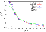
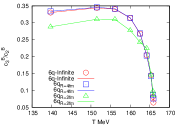
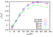
Figure 1: (Color online) Skewness for baryon fluctuation have been plotted with respect to collision centrality, baryon chemical potential and temperature. PNJL model with infinite volume has been denoted by red color, PNJL model with $R=4fm$ has been denoted by blue color and PNJL model with $R=2fm$ has been denoted by green color.

The correlation length and the magnitude of fluctuations are important quantity as they diverge at the critical end point. Because of the finite size and time effects, the correlation length takes a finite volume in the range $\sim 2-3fm$. Higher non-Gaussian moments such as skewness and kurtosis can provide much better handle in location of CEP as they are much more sensitive than variance to the correlation length. So the moment products have been constructed to cancel out volume dependence. In this figure panel 1, we have plotted the skewness of baryon fluctuation with respect to collision energy, temperature and baryon chemical potential for the PNJL model with infinite volume and also for the finite size with $R=2fm$ and $R=4fm$. The plots show a sharp rise near $\sqrt{s}=130GeV$, $\mu_{B}=36MeV$ and $T=165.8MeV$ for PNJL model with $R=2fm$ compared to other sets of the model. The sharp rise may be the indication of critical region. In figure 2 we have plotted the kurtosis for baryon fluctuation with respect to collision centrality, temperature and baryon chemical potentials. The kurtosis shows a minimum around $20-40GeV$ for collision centrality and a maximum around $40MeV$ for baryon chemical potential. Also it shows a sharp rise in temperature at $165MeV$. Both skewness and kurtosis of baryon fluctuations are in good agreement with the experimental result qualitatively STAR-proton .

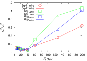
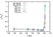
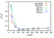
Figure 2: (Color online) Kurtosis for baryon fluctuation have been plotted with respect to collision centrality, baryon chemical potential and temperature. PNJL model with infinite volume has been denoted by red color, PNJL model with $R=4fm$ has been denoted by blue color and PNJL model with $R=2fm$ has been denoted by green color.

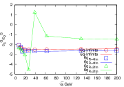
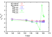
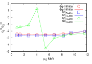
Figure 3: (Color online) Skewness for charge fluctuation have been plotted with respect to collision centrality, charge chemical potential and temperature. PNJL model with infinite volume has been denoted by red color, PNJL model with $R=4fm$ has been denoted by blue color and PNJL model with $R=2fm$ has been denoted by green color.

Figure 3 shows the skewness for charge fluctuation with respect to collision centrality, charge chemical potential and temperature. For $R=2fm$, the plots show a sharp rise around collision energy $20-40GeV$, temperature around $165MeV$ and chemical potential around $\mu_{Q}=4MeV$. The value of fluctuation is significantly large for $R=2fm$ than for $R=4fm$ and infinite volume. Figure 4 represents the kurtosis of charge fluctuation with respect to collision centrality, charge chemical potential and temperature. The kurtosis shows a minimum around $\sqrt{s}=20-40GeV$ for both finite and infinite volume. For temperature and charge chemical potential there is a sharp increase in fluctuation for both finite and infinte volume system. However the peaks are not in same position. It shifts to higher charge chemical potential and lower temperature for infinite volume system. For $R=2fm$ the peak is around $\mu_{Q}=5.5MeV$ and $T=163MeV$ and for infinite volume the peak is around $\mu_{Q}=8MeV$ and $T=155MeV$. Both the results for skewness and kurtosis are qualitatively similar to the experimental data STAR-charge .

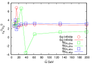
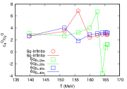
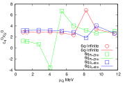
Figure 4: (Color online) Kurtosis for charge fluctuation have been plotted with respect to collision centrality, charge chemical potential and temperature. PNJL model with infinite volume has been denoted by red color, PNJL model with $R=4fm$ has been denoted by blue color and PNJL model with $R=2fm$ has been denoted by green color.

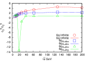
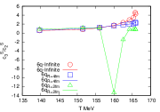
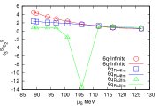
Figure 5: (Color online) Skewness for strangeness fluctuation have been plotted with respect to collision centrality, strangeness chemical potential and temperature. PNJL model with infinite volume has been denoted by red color, PNJL model with $R=4fm$ has been denoted by blue color and PNJL model with $R=2fm$ has been denoted by green color.

Figure (5) and (6) shows the variation of $C_{3}/C_{2_{S}}$ and $C_{4}/C_{2_{S}}$ fluctuations with respect to different collision energies, strangeness chemical potential and temperature for PNJL model. Skewness shows more fluctuation near $\sqrt{s}=20GeV$, $\mu_{S}=105MeV$ and $T=160MeV$. The fluctuation is more prominent for $R=2fm$. Kurtosis also shows similar kind of behaviour as skewness. In recent experimental data no significant deviation has been found with respect to the Poisson expectation value within statistical and systematic uncertainties for both the moments STAR-kaon . The results from the PNJL model are in good agreement with the experimental results. For the collision energy $\sqrt{s}<27\text{ GeV}$, there is an enhancement of fluctuation for PNJL model. Also in case of STAR results, there is an deviation from Poisson expectation value. Although the results for both skewness and kurtosis have qualitative similarities for PNJL model, the values have quantitative differences.

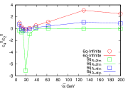
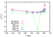
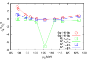
Figure 6: (Color online) Kurtosis for strangeness fluctuation have been plotted with respect to collision centrality, strangeness chemical potential and temperature. PNJL model with infinite volume has been denoted by red color, PNJL model with $R=4fm$ has been denoted by blue color and PNJL model with $R=2fm$ has been denoted by green color.

V summary

We have discussed properties of net baryon, charge and strangeness fluctuations in nuclear matter within finite size PNJL model. The ratio of fourth to second order moment and the third to the second order moment of fluctuations are considered as observables. All the correlations were obtained by fitting the pressure in a Taylor series expansion around the finite baryon, charge and strangeness chemical potentials. These chemical potentials are obtained from the freeze-out curve which depends on the collision energies in the BES scan at the heavy-ion collision experiment. The results are shown for PNJL model with 6 quark interactions and two finite volume systems with lateral size $R=2fm$ and $R=4fm$. We have considered the multiple reflection expansion method to include the surface and curvature effect of the fire ball along with the volume effect.

Skewness and kurtosis of baryon, charge and strangeness fluctuations in PNJL model have similar features along the collision energy of heavy ion experiments. As we increase the temperature both skewness and kurtosis value decreases quantitatively. For collision energy less than $27$ $GeV$, the value of kurtosis and skewness are higher. The recent experimental observations show small deviations for skewness and kurtosis for low collision energy. Similarly in PNJL model we have found an enhancement of fluctuations for low collision energy less than $27GeV$. Also, near the transition temperature the skewness ratio is very near to the Poisson expectation value.

The study of various equilibrium thermodynamic measurements of the correlators using PNJL model would be helpful in determining the finite temperature finite density behavior of the hadronic sector. comparison of PNJL results with the experimental value will ensure the understanding of the physics behind the critical region and to locate the critical point in the strongly interacting matter.

- (1) J. Adams et.al., Nucl. Phys. A 751 102–183 (2005).
- (2) M. M. Aggarwal et. al., Phys. Rev. C 82 024905 (2010).
- (3) Adronic et al., Nucl.Phys.A772:167 (2006).
- (4) B. Berdnikov and K. Rajagopal, Phys. Rev. D 61 105017 (2000).
- (5) M. Stephanov, K. Rajagopal and E. Shuryak, Phys. Rev. Lett. 81:4816–4819 (1998).
- (6) D. Adamova et. al., Phys. Rev. Lett. 90, 022301 (2003).
- (7) H.-T. Elze and W. Greiner, Phys. Lett. B 179, 385 (1986).
- (8) M. Luscher, Commun. Math. Phys. 104, 177 (1986).
- (9) J. Gasser and H. Leutwyler, Phys. Lett. B 188, 477 (1987).
- (10) Y. Nambu and G. Jona-Lasinio, Phys. Rev. 122, 345 (1961); 124, 246 (1961).
- (11) O. Kiriyama and A. Hosaka, Phys. Rev. D 67, 085010 (2003).
- (12) G. Shao, L. Chang, Y. Liu and X. Wang, Phys. Rev. D 73, 076003 (2006).
- (13) J. Braun, B. Klein and P. Piasecki, Eur. Phys. Jr. C 71, 1576 (2011).
- (14) J. Braun, B. Klein and B.-J. Schefer, Phys. Lett. B 713, 216 (2012).
- (15) A. Gopie and M. C. Ogilvie, Phys. Rev. D 59, 034009 (1999).
- (16) A. Bazavov and B. A. Berg, Phys. Rev. D 76, 014502 (2007).
- (17) A. Bhattacharyya, P. Deb, S. K. Ghosh, R. Ray, S. Sur, Phys.Rev. D 87 054009 (2013).
- (18) R. Balian and C. Bloch, Annals of Physics 60, 401, 1970.
- (19) J. Madsen, Phys. Rev. D 50, 3328 (1994).
- (20) O. Kiriyama, Phys. Rev. D 72, 054009 (2005).
- (21) A.G. Grunfeld and G. Lugones, Eur. Phys. J. C 78, 8, 640 (2018); G. Lugones and A. G. Grunfeld, Phys. Rev. C 95, 015804 (2017).
- (22) Y.P. Zhao, P.L. Yin, Z.h. Yu and H.S. Zong, Nucl. Phys. B. 952, 114919 (2020).
- (23) A. Bhattacharyya, R. Ray and S. Sur, Phys. rev. D 91 051501 (2005).
- (24) G. Boyd et. al., Nucl. Phys. B 469 419 (1996).
- (25) J. Engels et. al., Nucl. Phys. B 558 307 (1999).
- (26) Z. Fodor and S.D. Katz, Phys. Lett. B 534 87 (2002); Z. Fodor, S.D. Katz, and K.K. Szabo, Phys. Lett. B 568 73 (2003).
- (27) C.R. Allton, S. Ejiri, S.J. Hands, O. Kaczmarek, F. Karsch, E. Laermann, Ch. Schmidt, and L. Scorzato, Phys. Rev. D 66 074507 (2002); C.R. Allton, S. Ejiri, S.J. Hands, O. Kaczmarek, F.Karsch, E. Laermann, and Ch. Schmidt, Phys. Rev. D 68 014507 (2003); C.R. Allton, M. Doring, S. Ejiri, S.J. Hands, O. Kaczmarek, F. Karsch, E. Laermann, and K. Redlich, Phys. Rev. D 71 054508 (2005).
- (28) P. de Forcrand and O. Philipsen, Nucl. Phys. B642 290 (2002); B673 170 (2003).
- (29) Y. Aoki, Z. Fodor, S.D. katz, and K.K. Szabo, Phys. Lett.B 643 46 (2006); Y. Aoki, G. Endrodi, Z. Fodor, S.D. Katz, and K.K.Szabo, Nature (London) 443 675 (2006).
- (30) E. Megias, E. Ruiz Arriola, and L.L. Salcedo, Rom. Rep.Phys.58, 081 (2006); E. Megias, E.R. Arriola, and L.L. Salcedo, Proc. Sci., JHW2005 (2006) 025; E. Megias, E.R. Arriola, and L.L. Salcedo, Nucl. Phys. B, Proc. Suppl.186 256 (2009); E. Megias, E.R. Arriola, and L.L. Salcedo, Phys. Rev. D 81, 096009 (2010).
- (31) K. Fukushima, Phys. Lett. B 591 277 (2004).
- (32) C. Ratti, M.A. Thaler, and W. Weise, Phys. Rev. D 73 014019 (2006).
- (33) R.D. Pisarski, Phys. Rev. D 62 111501 (2000); A. Dumitru and R.D. Pisarski, Phys. Lett. B 504 282 (2001); 525 95 (2002); Phys. Rev. D 66 096003 (2002).
- (34) K. Fukushima, Phys. Rev. D 77 114028 (2008).
- (35) H. Hansen, W.M. Alberico, A. Beraudo, A. Molinari, M. Nardi, and C. Ratti, Phys. Rev. D 75 065004 (2007).
- (36) M. Ciminale, R. Gatto, N.D. Ippolito, G. Nardulli, and M. Ruggieri, Phys. Rev. D 77 054023 (2008).
- (37) S.K. Ghosh, T.K. Mukherjee, M.G. Mustafa, and R. Ray, Phys. Rev. D 73 114007 (2006); S.K. Ghosh, T.K. Mukherjee, M.G. Mustafa, and R. Ray, Phys. Rev. D 77 094024 (2008).
- (38) P. Deb, A. Bhattacharyya, S. Datta, and S.K. Ghosh,Phys. Rev. C 79 055208 (2009); A. Bhattacharyya, P. Deb, S. K.Ghosh, R. Ray, Phys. Rev. D 28 014021 (2010); A. Bhattacharyya, P. deb, A. Lahiri, R. Ray, Phys. Rev. D D 82 114028 (2010); A. Bhattacharyya, P. Deb, A. Lahiri, R. Ray, Phys. Rev. D 83 014011 (2011).
- (39) A.A. Osipov, B. Hiller, and J. da Providencia, Phys. Lett. B 634, 48 (2006); A.A. Osipov, B. Hiller, V. Bernard, and A.H. Blin, Ann. Phys. (N.Y.) 321, 2504 (2006); A.A. Osipov, B. Hiller, A.H. Blin, and J. da Providencia, Ann. Phys. (N.Y.) 322, 2021 (2007); B. Hiller, J. Moreira, A.A. Osipov, and A.H. Blin, Phys. Rev. D 81, 116005 (2010).
- (40) K. Kashiwa, H. Kouno, T. Sakagauchi, M. Matsuzaki, and M. Yahiro, Phys. Lett. B 647, 446 (2007), K. Kashiwa, H. Kouno, M. Matsuzaki, and M. Yahiro, Phys. Lett. B 662, 26 (2008).
- (41) B. J. Schaefer and J. Wambach, Phys. Rev. D 75, 085015 (2007), B.J. Schaefer, J.M. Pawlowski, and J. Wambach, Phys. Rev. D 76, 074023 (2007), B.J. Schaefer, M. Wagner, and J. Wambach, Phys. Rev. D 81, 074013 (2010), J. Wambach, B.J. Schaefer, and M. Wagner, Acta Phys. Polon. Supp. 3 , 691 (2010); V. Skokov, B. Friman, E. Nakano, K. Redlich, and B. J. Schaefer, Phys. Rev. D 82, 034029 (2010).
- (42) P. Chakraborty, M.G. Mustafa, and M.H. Thoma, Eur. Phys. J. C 23, 591 (2002); P. chakraborty, M. G. Mustafa, M. H. Thoma, Phys. Rev. D 68, 0855012 (2003); N. Haque, M. G. Mustafa, arXiv:1007.2076.
- (43) S. Ejiri, F. Karsch, and K. Redlich, Phys. Lett. B 633, 275 (2006).
- (44) S. Roessner, C. Ratti, and W. Weise, Phys. Rev. D 75, 034007 (2007); C. Sasaki, B. Friman, and K. Redlich, Phys. Rev. D 75, 074013 (2007); S. Mukherjee, M. G. Mustafa, and R. Ray, Phys. Rev. D 75, 094015 (2007).
- (45) A. Bhattacharyya, S. K. Ghosh, R. Ray, K. Saha and S. Upadhaya, Eur. Phys. Lett. 116 5 52001 (2016).
- (46) M. Cheng et. al., Phys. Rev. D 77, 014511 (2008); M. Cheng et. al., Phys. Rev. D 79, 074505 (2009).
- (47) A. Bazavov et. al., Phys. Rev. D 85 054503 (2012).
- (48) A. Bazavov et. al., Phys. Rev. D 90 094503 (2014).
- (49) S. Borsanyi et. al., Phys. Lett. B 730 99 (2014).
- (50) A. Bhattacharyya, S. K. Ghosh, S. Maity, S. Raha, R. Ray, K. Saha and S. Upadhaya, Phys. Rev. D 95 5 054005 (2017).
- (51) P. B. Munzinger, D. Magestro, K. Redlich and J. Stachel, Phys. Lett. B 518 41–46 (2001).
- (52) A. Andronic, P. B. Munzinger and J. Stachel, Phys. Lett. B 673 142–145 (2009).
- (53) J. Cleymans, H. Oeschler, K. Redlich and S. Wheaton, Phys. Rev.C 73034905 (2006).
- (54) F. Karsch and K. Redlich, Phys. Lett. B 695 136-142 (2011).
- (55) http://www.gnuplot.info/
- (56) C. S. Fischer and M. R. Pennington, Phys. Rev. D 73, 034029 (2006).
- (57) J. Luecker, C. S. Fischer and R Williams, Phys. Rev. D 81, 094005 (2010).
- (58) F. C. Khanna, A. P. C. Malbouisson, J. M. C. Malbouisson and A. E. Santana, Eur. Phys. Lett. 97, 11002 (2012).
- (59) S. Yasui and A. Hosaka, Phys. Rev. D 74, 054036 (2006).
- (60) L. M. Abreu, A. P. C. Malbouisson and J. M. C. Malbouisson, Phys. Rev. D 83, 025001 (2011); L. M. Abreu, A. P. C. Malbouisson and J. M. C. Malbouisson, Phys. Rev. D 84, 065036 (2011).
- (61) D. Ebert, T. G. Khunjua, K. G. Klimenko and V. Ch. Zhukovsky, Int. Jr. Mod. Phys. A 27, 1250162 (2012).
- (62) B. A. Berg and H. Wu, Phys. Rev. D 88, 074507 (2013).
- (63) L. Adamczyk et. al, Phys. Rev. Lett. 112, 032302 (2014).
- (64) L. Adamczyk et. al, Phys. Rev. Lett. 113, 092301 (2014).
- (65) L. Adamczyk et. al, Phys. Lett. B 785, 551-560 (2018).
- (66) J. Thader, Nucl. Phys. A 00, 1-4 (2016).
- (67) K. Fukushima, Phys. Rev. D 79, 074015 (2009).