ADMM based Distributed State Observer Design under Sparse Sensor Attacks

Vinaya Mary Prinse and Rachel Kalpana Kalaimani The authors are with the Department of Electrical Engineering, Indian Institute of Technology Madras, Chennai 600036 India (email: ee20s021@smail.iitm.ac.in, rachel@ee.iitm.ac.in).
Abstract

This paper considers the design of a distributed state-observer for discrete-time Linear Time Invariant (LTI) systems in the presence of sensor attacks. We assume there is a network of observer nodes, communicating with each other over an undirected graph, each with partial measurements of the output corrupted by some adversarial attack. We address the case of sparse attacks where the attacker targets a small subset of sensors. An algorithm based on Alternating Direction Method of Multipliers (ADMM) is developed which provides an update law for each observer which ensures convergence of each observer node to the actual state asymptotically.

Index Terms:
Distributed observers, cyber-physical systems, secure state estimation, sparse sensor attacks, ADMM.

I Introduction

Over the past few decades, a distributed approach is being adopted for large scale and complex Cyber-Physical Systems (CPSs) such as smart grids, industrial control systems, robotic systems etc. to enhance flexibility, robustness and computational performance. However, the susceptibility of these systems to attacks is a reality as highlighted in [1] and [2] and a few examples include the Ukrainian power grid hack[3], the worldwide Wannacry ransomware attack and the Stuxnet attack [4]. Hence, the security of CPSs is of primary concern.

We consider the problem of estimating the state of linear dynamical systems when few sensors are corrupted, called sparse sensor attacks. We adopt a distributed approach for an observer design and assume a network of observers where each observer has access to partial measurements of the output. Since each observer need not be observable, state estimation by the observers require communication with each other.

A centralized state observer for Linear Time Invariant (LTI) systems under sparse sensor attacks is proposed in [5] and [6] considers sparse actuator attacks also. Design of a distributed observer for state estimation without sensor attacks is discussed in [7] for discrete time LTI systems and in [8] for continuous time LTI systems.

While an observer is a dynamic process, which uses new measurements to update the current state value, a static approach is to just estimate the initial condition using a batch of measurements and then use the system dynamics to construct the current state. Now, additionally when there are sensor attacks, estimating the state using the above static approach is known as Secure State Estimation (SSE) problem in literature. When a distributed approach is used, the above problem is referred to as Distributed SSE (DSSE) where each agent estimates the initial state based on its own (limited) state measurements and the information from neighbours despite sparse sensor attacks. DSSE has been addressed in [9] and [10]. The latter has an additional sparsity assumption on the initial state. DSSE with secure preselectors is discussed in [11] but has a complicated parameter design as mentioned in [4].

A distributed observer for LTI systems with Byzantine attacks is studied in [12]. In Byzantine attacks, adversaries are allowed to send differing state estimates to different neighbors at the same instant of time, State estimation for this kind of adversaries is addressed for stronger assumptions on the network graph. We consider a simpler case, where the attacker tampers only a few measurements of the system and therefore require a comparatively weaker assumption of just the graph being connected.

A distributed observer design in case of sparse attacks is proposed in [13] for linear continuous time systems. This involves an attack indicator signal with exponential computational complexity. We propose a distributed observer design, for discrete time LTI systems, under sparse sensor attacks. The main contributions of our work are as follows:

  1. 1.

    Design a distributed observer when there are sparse sensor attacks. An algorithm based on Alternating Direction Method of Multipliers (ADMM) is used to update each observer.

  2. 2.

    The DSSE can be recovered as a special case of the above algorithm. We compare this with the DSSE algorithm in [10].

  3. 3.

    We also compare the centralized implementation of our algorithm with [5] which discusses a centralized state observer under sparse sensor attacks.

I-A Notation

,\mathbb{N,R} denote the set of natural and real numbers respectively. Γ¯¯Γ\bar{\Gamma} denotes complement of a set ΓΓ\Gamma. bTsuperscript𝑏𝑇b^{T} represents transpose of vector b𝑏b. Insubscript𝐼𝑛I_{n} is the identity matrix of dimension n𝑛n. For a vector yn𝑦superscript𝑛y\in\mathbb{R}^{n}, l0subscript𝑙0l_{0} norm of y𝑦y i.e. y0subscriptnorm𝑦0\|y\|_{0} refers to the number of nonzero components in y𝑦y and yrsubscriptnorm𝑦𝑟\|y\|_{r} represents r norm of y𝑦y. (x,y)𝑥𝑦(x,y) denotes the vector [xTyT]Tn1×n2superscriptdelimited-[]superscript𝑥𝑇superscript𝑦𝑇𝑇superscriptsubscript𝑛1superscriptsubscript𝑛2[x^{T}\hskip 5.16663pty^{T}]^{T}\subset\mathbb{R}^{n_{1}}\times\mathbb{R}^{n_{2}} where xn1𝑥superscriptsubscript𝑛1x\in\mathbb{R}^{n_{1}} and yn2𝑦superscriptsubscript𝑛2y\in\mathbb{R}^{n_{2}}.

|K|𝐾|K| represents cardinality of a set K𝐾K. A vector xn𝑥superscript𝑛x\in\mathbb{R}^{n} is said to be s𝑠s sparse when |supp(x)|s𝑠𝑢𝑝𝑝𝑥𝑠|supp(x)|\leq s. A block vector given by y=(y1,,yp)pτ𝑦subscript𝑦1subscript𝑦𝑝superscript𝑝𝜏y=(y_{1},...,y_{p})\in\mathbb{R}^{p\tau}, where y1,,ypτsubscript𝑦1subscript𝑦𝑝superscript𝜏y_{1},...,y_{p}\in\mathbb{R}^{\tau} are blocks, is block s𝑠s-sparse if at most s𝑠s blocks are nonzero. We use s𝑠s-sparse instead of the term block s𝑠s-sparse and 𝕊spτpτsuperscriptsubscript𝕊𝑠𝑝𝜏superscript𝑝𝜏\mathbb{S}_{s}^{p\tau}\subset\mathbb{R}^{p\tau} denotes the set of these vectors.

An undirected graph is represented by 𝒢=(𝒱,,𝒜)𝒢𝒱𝒜\mathcal{G}=(\mathcal{V,E,A}) where 𝒱={1,2,..,N}\mathcal{V}=\{1,2,..,N\} is the vertex set, 𝒱×𝒱𝒱𝒱\mathcal{E}\subset\mathcal{V}\times\mathcal{V} is the undirected edge set and 𝒜={aij}N×N𝒜subscriptsubscript𝑎𝑖𝑗𝑁𝑁\mathcal{A}=\{a_{ij}\}_{N\times N} is the adjacency matrix where aij=1subscript𝑎𝑖𝑗1a_{ij}=1 if (i,j)𝑖𝑗(i,j)\in\mathcal{E} i.e. it indicates that nodes i𝑖i and j𝑗j are connected, else aij=0subscript𝑎𝑖𝑗0a_{ij}=0. We will assume a graph without loops or multiple edges i.e. aii=0subscript𝑎𝑖𝑖0a_{ii}=0. The neighbourhood set of the i𝑖ith node is defined as i={j:(i,j)}subscript𝑖conditional-set𝑗𝑖𝑗\mathbb{N}_{i}=\{j:(i,j)\in\mathcal{E}\}. A graph is said to be connected if there exists a path to traverse between every pair of distinct nodes i𝑖i and j𝑗j in 𝒢𝒢\mathcal{G}.

Hereafter the paper organization is as follows. Section II formally states the problem objective. The main results of this paper are given in Section III which includes optimization problem reformulation followed by the distributed observer design and simulation results for DSSE and centralized observer implementations in addition. The paper is concluded in section IV.

II Problem Formulation

Consider the following discrete-time LTI system, whose measurements are corrupted.

x[t+1]𝑥delimited-[]𝑡1\displaystyle x[t+1] =\displaystyle= Ax[t]+Bu[t],𝐴𝑥delimited-[]𝑡𝐵𝑢delimited-[]𝑡\displaystyle Ax[t]+Bu[t],
y[t]𝑦delimited-[]𝑡\displaystyle y[t] =\displaystyle= Cx[t]+a[t],𝐶𝑥delimited-[]𝑡𝑎delimited-[]𝑡\displaystyle Cx[t]+a[t], (1)

where x[t]n𝑥delimited-[]𝑡superscript𝑛x[t]\in\mathbb{R}^{n} is the state vector, y[t]p𝑦delimited-[]𝑡superscript𝑝y[t]\in\mathbb{R}^{p} is the measurement vector and a[t]p𝑎delimited-[]𝑡superscript𝑝a[t]\in\mathbb{R}^{p} is the s𝑠s sparse attack vector assuming that at most s𝑠s sensors are attacked. The objective is to construct a distributed observer for the above system which estimates the system state and attack vector (thereby the set of corrupted sensors) at time t𝑡t by communication within the network.

It is well known that a sufficient condition which guarantees exact state estimation despite an s𝑠s sparse sensor attack is the 2s2𝑠2s-sparse observability condition [5]. A system is said to be s𝑠s-sparse observable if the system remains observable even after removing any s𝑠s sensors i.e. for every set Γ{1,..,p}\Gamma\subset\{1,..,p\} with |Γ|=sΓ𝑠|\Gamma|=s, the observability matrix of (A,CΓ¯)𝐴subscript𝐶¯Γ(A,C_{\bar{\Gamma}}) has full rank (CΓ¯subscript𝐶¯ΓC_{\bar{\Gamma}} indicates the matrix resulting on elimination of rows indexed by ΓΓ\Gamma from C𝐶C).

For the distributed framework, we assume that there are N𝑁N local observers (or agents) each with a set of sensors which measures a part of the output, yi[t]pisubscript𝑦𝑖delimited-[]𝑡superscriptsubscript𝑝𝑖y_{i}[t]\in\mathbb{R}^{p_{i}}, i=1Npi=psuperscriptsubscript𝑖1𝑁subscript𝑝𝑖𝑝\sum_{i=1}^{N}p_{i}=p. This measurement is corrupted by ai[t]pisubscript𝑎𝑖delimited-[]𝑡superscriptsubscript𝑝𝑖a_{i}[t]\in\mathbb{R}^{p_{i}}. The communication network is depicted by a graph, whose vertices represent the observers and edges represent the existence of a communication channel between two observers. Using the partial, corrupted measurement and additionally communicating with its neighbours, each observer should be able to estimate the state vector of the system in (II).

Next we list the assumptions on our system model:

Assumption 1
  1. 1.

    The graph representing the communication network of the distributed observers is connected.

  2. 2.

    The system (A,C)𝐴𝐶(A,C) is 2s2𝑠2s-sparse observable

  3. 3.

    The attack vector a[t]𝑎delimited-[]𝑡a[t] is s𝑠s sparse (provided s<p2𝑠𝑝2s<\frac{p}{2} [14])

The set of corrupted sensors is assumed to be fixed over time. However, it is important to note that the effect of the attack is propagated to the neighboring observers of a local observer receiving corrupted sensor measurements, through the communication network. Next we formally state our problem of designing a distributed observer under sensor attacks.

Problem 1

Consider a set of N𝑁N agents/observers, each with partial and corrupted measurements of the output, interacting with each other to estimate the state of the system in (II), satisfying conditions in Assumption 1. Let xi~[t]n~subscript𝑥𝑖delimited-[]𝑡superscript𝑛\tilde{x_{i}}[t]\in\mathbb{R}^{n} denote an estimate of the state that an observer i𝑖i has at time t𝑡t. Design an update law for each agent, that can be implemented in a distributed manner, such that the following holds:

limtxi~[t]x[t]0,i𝑡limnorm~subscript𝑥𝑖delimited-[]𝑡𝑥delimited-[]𝑡0for-all𝑖\underset{t\rightarrow\infty}{\mbox{lim}}\|\tilde{x_{i}}[t]-x[t]\|\rightarrow 0,~{}\forall~{}i

III Results

III-A Optimization Formulation

In [5], in order to obtain an observer, an optimization problem is formulated first and then recursively solved. We follow a similar approach to get a distributed observer. By collecting the sequence of last τ𝜏\tau observed outputs (τ,τnformulae-sequence𝜏𝜏𝑛\tau\in\mathbb{N},\tau\leq n) at time tτ𝑡𝜏t\geq\tau, a delayed version of the system state i.e. x[tτ+1]𝑥delimited-[]𝑡𝜏1x[t-\tau+1] can be reconstructed.

Let Ej[t]τsubscript𝐸𝑗delimited-[]𝑡superscript𝜏E_{j}[t]\in\mathbb{R}^{\tau} denote the vector of attack signals on the j𝑗jth sensor from time tτ+1𝑡𝜏1t-\tau+1 to t𝑡t, i.e. Ej[t]=(aj[tτ+1],,aj[t])subscript𝐸𝑗delimited-[]𝑡subscript𝑎𝑗delimited-[]𝑡𝜏1subscript𝑎𝑗delimited-[]𝑡E_{j}[t]=(a_{j}[t-\tau+1],...,a_{j}[t]). This vector is stacked for all sensors to obtain E[t]𝐸delimited-[]𝑡E[t] i.e. E[t]=(E1[t],,Ep[t])𝐸delimited-[]𝑡subscript𝐸1delimited-[]𝑡subscript𝐸𝑝delimited-[]𝑡E[t]=(E_{1}[t],...,E_{p}[t]). The attack signal on the j𝑗jth sensor, aj[t]subscript𝑎𝑗delimited-[]𝑡a_{j}[t], can be expressed as

aj[t]=yj[t]Cjx[t]subscript𝑎𝑗delimited-[]𝑡subscript𝑦𝑗delimited-[]𝑡subscript𝐶𝑗𝑥delimited-[]𝑡a_{j}[t]=y_{j}[t]-C_{j}x[t] (2)

Hence, if we have an estimate of x[tτ+1]𝑥delimited-[]𝑡𝜏1x[t-\tau+1], then using the above equation (2) and the system dynamics in (II), we can obtain an estimate of the state and attack vectors from time tτ+1𝑡𝜏1t-\tau+1 to t𝑡t.

Consider the vector z(t)𝑧𝑡z(t) defined as z[t]=(x[t],E[t])𝑧delimited-[]𝑡𝑥delimited-[]𝑡𝐸delimited-[]𝑡z[t]=(x[t],E[t]). Let Y¯(t)pτ¯𝑌𝑡superscript𝑝𝜏\bar{Y}(t)\in\mathbb{R}^{p\tau} denote the set of past τ𝜏\tau outputs collected for all the sensors i.e. Y¯[t]=(Y¯1[t],,Y¯p[t])¯𝑌delimited-[]𝑡subscript¯𝑌1delimited-[]𝑡subscript¯𝑌𝑝delimited-[]𝑡\bar{Y}[t]=(\bar{Y}_{1}[t],...,\bar{Y}_{p}[t]) where Y¯j[t]=(yj[tτ+1],,yj[t])subscript¯𝑌𝑗delimited-[]𝑡subscript𝑦𝑗delimited-[]𝑡𝜏1subscript𝑦𝑗delimited-[]𝑡\bar{Y}_{j}[t]=(y_{j}[t-\tau+1],...,y_{j}[t]). Then from [5], we obtain the dynamics of z(t)𝑧𝑡z(t) and a relation between Y¯(t)¯𝑌𝑡\bar{Y}(t) and z(t)𝑧𝑡z(t) as follows:

z[t]𝑧delimited-[]𝑡\displaystyle z[t] =\displaystyle= A¯z[t1]+Ny[t]¯𝐴𝑧delimited-[]𝑡1𝑁𝑦delimited-[]𝑡\displaystyle\bar{A}z[t-1]+Ny[t] (3)
Y¯[t]¯𝑌delimited-[]𝑡\displaystyle\bar{Y}[t] =\displaystyle= Qz[t]𝑄𝑧delimited-[]𝑡\displaystyle Qz[t] (4)

where A¯=[A00G1S0Gp0S]¯𝐴delimited-[]𝐴00subscript𝐺1𝑆0missing-subexpressionmissing-subexpressionsubscript𝐺𝑝0𝑆\bar{A}=\left[\begin{smallmatrix}A&0&\cdots{}&0\\ G_{1}&S&\cdots{}&0\\ \vdots{}&&\ddots{}&\\ G_{p}&0&\cdots{}&S\end{smallmatrix}\right], Q=[O1IpτOp]𝑄delimited-[]subscript𝑂1missing-subexpressionsubscript𝐼𝑝𝜏subscript𝑂𝑝missing-subexpression~{}Q=\left[\begin{smallmatrix}O_{1}&\\ \vdots{}&I_{p\tau}\\ O_{p}&\end{smallmatrix}\right]~{} and N=[0N1Np]𝑁delimited-[]0subscript𝑁1subscript𝑁𝑝~{}N=\left[\begin{smallmatrix}0\\ N_{1}\\ \vdots{}\\ N_{p}\end{smallmatrix}\right]. Here, Gj=[00CjAτ]subscript𝐺𝑗delimited-[]00subscript𝐶𝑗superscript𝐴𝜏G_{j}=\left[\begin{smallmatrix}0\\ \vdots{}\\ 0\\ -C_{j}A^{\tau}\end{smallmatrix}\right], S=[0100010001000]𝑆delimited-[]0100010missing-subexpressionmissing-subexpression001000S=\left[\begin{smallmatrix}0&1&\cdots{}&\cdots{}&0\\ 0&0&1&\cdots{}&0\\ \vdots{}&\vdots{}&&\ddots{}&\\ 0&0&\cdots{}&\cdots{}&1\\ 0&0&\cdots{}&\cdots{}&0\end{smallmatrix}\right] and Nj=[00bj]subscript𝑁𝑗delimited-[]00subscript𝑏𝑗N_{j}=\left[\begin{smallmatrix}0\\ \vdots{}\\ 0\\ b_{j}\end{smallmatrix}\right] where bjsubscript𝑏𝑗b_{j} represents the j𝑗jth standard basis vector and Oj=[CjT(CjA)T(CjAτ1)T]Tsubscript𝑂𝑗superscriptdelimited-[]superscriptsubscript𝐶𝑗𝑇superscriptsubscript𝐶𝑗𝐴𝑇superscriptsubscript𝐶𝑗superscript𝐴𝜏1𝑇𝑇O_{j}=\left[\begin{array}[]{cccc}C_{j}^{T}&(C_{j}A)^{T}&\ldots{}&(C_{j}A^{\tau-1})^{T}\end{array}\right]^{T}.

Since we are interested in an observer, for simplifying the analysis, we ignore the external input in the system dynamics. Let x~[t]~𝑥delimited-[]𝑡\tilde{x}[t] denote the estimate of x[tτ+1]𝑥delimited-[]𝑡𝜏1x[t-\tau+1] and E~[t]~𝐸delimited-[]𝑡\tilde{E}[t] denote the estimate of E[t]𝐸delimited-[]𝑡E[t]. Then estimate of z[t]𝑧delimited-[]𝑡z[t] denoted as z~[t]~𝑧delimited-[]𝑡\tilde{z}[t] is the vector (x~[t],E~[t])~𝑥delimited-[]𝑡~𝐸delimited-[]𝑡(\tilde{x}[t],\tilde{E}[t]).

In order to obtain the estimate z~(t)~𝑧𝑡\tilde{z}(t) at a given time t𝑡t, the following optimization problem is solved:

minz~n×𝕊spτ12Y¯[t]Qz~[t]22~𝑧superscript𝑛superscriptsubscript𝕊𝑠𝑝𝜏12superscriptsubscriptnorm¯𝑌delimited-[]𝑡𝑄~𝑧delimited-[]𝑡22\underset{\tilde{z}\in\mathbb{R}^{n}\times\mathbb{S}_{s}^{p\tau}}{\min}\frac{1}{2}\|\bar{Y}[t]-Q\tilde{z}[t]\|_{2}^{2} (5)

Note that E~~𝐸\tilde{E} part of the variable z~~𝑧\tilde{z} in the above optimization problem is constrained to be in 𝕊spτsuperscriptsubscript𝕊𝑠𝑝𝜏\mathbb{S}_{s}^{p\tau} due to the sparse structure of the attack vector. According to Theorem 3.2 in [5], for a 2s2𝑠2s-sparse observable system, this problem has a unique minimum, (x,E)superscript𝑥superscript𝐸(x^{*},E^{*}) in the set n×𝕊spτsuperscript𝑛superscriptsubscript𝕊𝑠𝑝𝜏\mathbb{R}^{n}\times\mathbb{S}_{s}^{p\tau}. Hence, this problem is reformulated as an l0subscript𝑙0l_{0} norm minimization problem for E~~𝐸\tilde{E}. The optimal solution, which is the most sparse E~~𝐸\tilde{E} will be the unique s𝑠s-sparse vector Esuperscript𝐸E^{*} in this case. Thus, the sparse nature of the attack vector is utilised to reformulate the above problem into the following l0subscript𝑙0l_{0} norm optimization problem A𝐴A:

A:minz~=(x~,E~)E~0s.t.Qz~=Y¯A:\underset{\tilde{z}=(\tilde{x},\tilde{E})}{\min}\|\tilde{E}\|_{0}\hskip 4.30554pts.t.\hskip 4.30554ptQ\tilde{z}=\bar{Y} (6)

Note that problem A𝐴A is not convex. Hence we consider the following convex relaxation of problem A𝐴A known as the basis pursuit problem:

B:minz~=(x~,E~)E~1s.t.Qz~=Y¯B:\underset{\tilde{z}=(\tilde{x},\tilde{E})}{\min}\|\tilde{E}\|_{1}\hskip 4.30554pts.t.\hskip 4.30554ptQ\tilde{z}=\bar{Y} (7)

The following lemma provides a condition when the two problems are equivalent. [14, Proposition 6] and [15, Proposition 3] discuss similar conditions and hence we skip the proof.

Lemma 1

Let (x~0,E~0)subscript~𝑥0subscript~𝐸0(\tilde{x}_{0},\tilde{E}_{0}) and (x~1,E~1)subscript~𝑥1subscript~𝐸1(\tilde{x}_{1},\tilde{E}_{1}) be the solutions to the optimization problems A𝐴A and B𝐵B respectively. Then for a 2s2𝑠2s-sparse observable system, the following are equivalent:

  1. 1.

    (x~1,E~1)=(x~0,E~0)subscript~𝑥1subscript~𝐸1subscript~𝑥0subscript~𝐸0(\tilde{x}_{1},\tilde{E}_{1})=(\tilde{x}_{0},\tilde{E}_{0})

  2. 2.

    For all Γ{1,,p}Γ1𝑝\Gamma\subset\{1,...,p\} with |Γ|=sΓ𝑠|\Gamma|=s, the following holds:

    iΓ|(Ox~)i|<iΓ¯|(Ox~)i|,x~n{0}formulae-sequencesubscript𝑖Γsubscript𝑂~𝑥𝑖subscript𝑖¯Γsubscript𝑂~𝑥𝑖for-all~𝑥superscript𝑛0\sum_{i\in\Gamma}|(O\tilde{x})_{i}|<\sum_{i\in\bar{\Gamma}}|(O\tilde{x})_{i}|,~{}\forall~{}\tilde{x}\in\mathbb{R}^{n}\char 92\relax\{0\} (8)

    where O=[O1TOpT]T𝑂superscriptdelimited-[]superscriptsubscript𝑂1𝑇superscriptsubscript𝑂𝑝𝑇𝑇O=[O_{1}^{T}~{}~{}\cdots{}~{}~{}O_{p}^{T}]^{T} is part of the Q𝑄Q in (4).

These results are utilised to reformulate the optimization problem in (5) into a basis pursuit problem in the following theorem.

Theorem 1

Let the discrete time LTI system defined in (II) be 2s2𝑠2s-sparse observable. Then the optimization problems in (5) and (7) are equivalent provided condition (8) holds Γ{1,,p}for-allΓ1𝑝\forall~{}\Gamma\subset\{1,...,p\} with |Γ|=sΓ𝑠|\Gamma|=s.

The proof is straightforward from the re-formulated optimization problem A in (6) and Lemma 1. \hfill\blacksquare

Problem B𝐵B needs to be formulated in a distributed set up in order to address our main objective of proposing a distributed observer. Each local observer in the network will have access to a part of the measurements of the system and collection of these measurements from time tτ+1𝑡𝜏1t-\tau+1 to t𝑡t gives Yi[t]subscript𝑌𝑖delimited-[]𝑡Y_{i}[t] for the i𝑖ith observer. Now an observer/agent i𝑖i can have an estimate of the state vector x[tτ+1]𝑥delimited-[]𝑡𝜏1x[t-\tau+1] and of the attack vector corresponding to the measurements received by them denoted by xi~[t]~subscript𝑥𝑖delimited-[]𝑡\tilde{x_{i}}[t] and 𝔼i~[t]~subscript𝔼𝑖delimited-[]𝑡\tilde{\mathbb{E}_{i}}[t] respectively. Similar to the output equation given in (4), the output equation for observer i𝑖i can be written as follows:

Yi[t]=[O1+j=1i1pjIpiτOpi+j=1i1pj][xi~[t]𝔼~i[t]]=Qizi~[t]subscript𝑌𝑖delimited-[]𝑡delimited-[]subscript𝑂1superscriptsubscript𝑗1𝑖1subscript𝑝𝑗missing-subexpressionsubscript𝐼subscript𝑝𝑖𝜏subscript𝑂subscript𝑝𝑖superscriptsubscript𝑗1𝑖1subscript𝑝𝑗missing-subexpressiondelimited-[]~subscript𝑥𝑖delimited-[]𝑡subscript~𝔼𝑖delimited-[]𝑡subscript𝑄𝑖~subscript𝑧𝑖delimited-[]𝑡\begin{split}Y_{i}[t]&=\left[\begin{array}[]{cc}O_{1+\sum_{j=1}^{i-1}p_{j}}&\\ \vdots{}&I_{p_{i}\tau}\\ O_{p_{i}+\sum_{j=1}^{i-1}p_{j}}&\end{array}\right]\left[\begin{array}[]{c}\tilde{x_{i}}[t]\\ \tilde{\mathbb{E}}_{i}[t]\end{array}\right]=Q_{i}\tilde{z_{i}}[t]\end{split} (9)

where 𝔼~i[t]subscript~𝔼𝑖delimited-[]𝑡\tilde{\mathbb{E}}_{i}[t] is a vector extracted from E~[t]~𝐸delimited-[]𝑡\tilde{E}[t] corresponding to the attack on observer i and Qisubscript𝑄𝑖Q_{i} refers to the matrix in the above equation. Each agent gets an estimate of the initial condition and attack vectors, zi~[t]=(xi~[t],𝔼i~[t])~subscript𝑧𝑖delimited-[]𝑡~subscript𝑥𝑖delimited-[]𝑡~subscript𝔼𝑖delimited-[]𝑡\tilde{z_{i}}[t]=(\tilde{x_{i}}[t],\tilde{\mathbb{E}_{i}}[t]), by a distributed approach. In this regard, an optimization problem that is equivalent to B𝐵B is formulated in the following Lemma.

Lemma 2

The optimization problem B𝐵B in (7) is equivalent to the following optimization problem:

minzi~=(xi~,𝔼~i),bi𝔼~11+𝔼~21++𝔼~N1~subscript𝑧𝑖~subscript𝑥𝑖subscript~𝔼𝑖subscript𝑏𝑖subscriptnormsubscript~𝔼11subscriptnormsubscript~𝔼21subscriptnormsubscript~𝔼𝑁1\displaystyle\underset{\tilde{z_{i}}=(\tilde{x_{i}},\tilde{\mathbb{E}}_{i}),b_{i}}{\min}\|\tilde{\mathbb{E}}_{1}\|_{1}+\|\tilde{\mathbb{E}}_{2}\|_{1}+...+\|\tilde{\mathbb{E}}_{N}\|_{1} (10)
s.t.Qizi~=Yii=1,,Nformulae-sequence𝑠𝑡subscript𝑄𝑖~subscript𝑧𝑖subscript𝑌𝑖for-all𝑖1𝑁\displaystyle s.t.\hskip 4.30554ptQ_{i}\tilde{z_{i}}=Y_{i}\hskip 4.30554pt\forall i=1,...,N
xi~=bj,(i,j)formulae-sequence~subscript𝑥𝑖subscript𝑏𝑗for-all𝑖𝑗\displaystyle\tilde{x_{i}}=b_{j},\hskip 4.30554pt\forall(i,j)\in\mathcal{E}
xi~=bi,i=1,,Nformulae-sequence~subscript𝑥𝑖subscript𝑏𝑖for-all𝑖1𝑁\displaystyle\tilde{x_{i}}=b_{i},\hskip 4.30554pt\forall i=1,...,N

where Qisubscript𝑄𝑖Q_{i} is defined in (9) and bisubscript𝑏𝑖b_{i} is an auxiliary variable.

Proof: In problem B𝐵B, the objective function E~1subscriptnorm~𝐸1\|\tilde{E}\|_{1} can be written as the sum of 𝔼~i1subscriptnormsubscript~𝔼𝑖1\|\tilde{\mathbb{E}}_{i}\|_{1}s by definition of one norm. The constraint Qz~=Y¯𝑄~𝑧¯𝑌Q\tilde{z}=\bar{Y}, is decomposed for each observer i𝑖i in (9). Consequently, each observer maintains its own estimate of the initial condition, xi~~subscript𝑥𝑖\tilde{x_{i}}. Next, to enforce consensus on the state estimates i.e. to achieve x1~==xN~~subscript𝑥1~subscript𝑥𝑁\tilde{x_{1}}=...=\tilde{x_{N}} in a distributed/parallel manner, we need to introduce auxiliary variables. We adopt the approach proposed in [16] which uses one auxiliary variable per node, say bisubscript𝑏𝑖b_{i}. Then the consensus constraint equations can be written as xi~=bj(i,j)~subscript𝑥𝑖subscript𝑏𝑗for-all𝑖𝑗\tilde{x_{i}}=b_{j}\hskip 4.30554pt\forall(i,j)\in\mathcal{E} and xi~=bii=1,,Nformulae-sequence~subscript𝑥𝑖subscript𝑏𝑖for-all𝑖1𝑁\tilde{x_{i}}=b_{i}\hskip 4.30554pt\forall i=1,...,N. Since the objective function and constraints are equivalent, the optimization problems given in (7) and (10) are equivalent. \hfill\blacksquare

III-B Distributed Observer

In this section, we first propose an ADMM based algorithm, that can be implemented in a distributed manner, to solve the optimization problem formulated in Lemma 2. Then for the observer, a suitable recursive implementation is proposed incorporating new measurements at each time.

Consider the augmented Lagrangian for the optimization problem given in (10) (by dualizing only the consensus constraints) :

ρ=i=1N(Ei~1+j𝒩iλijT(xi~bj)+ρ2j𝒩ixi~bj2+λiiT(xi~bi)+ρ2xi~bi2)subscript𝜌superscriptsubscript𝑖1𝑁subscriptdelimited-∥∥~subscript𝐸𝑖1subscript𝑗subscript𝒩𝑖superscriptsubscript𝜆𝑖𝑗𝑇~subscript𝑥𝑖subscript𝑏𝑗𝜌2subscript𝑗subscript𝒩𝑖superscriptdelimited-∥∥~subscript𝑥𝑖subscript𝑏𝑗2superscriptsubscript𝜆𝑖𝑖𝑇~subscript𝑥𝑖subscript𝑏𝑖𝜌2superscriptdelimited-∥∥~subscript𝑥𝑖subscript𝑏𝑖2\mathcal{L}_{\rho}=\sum_{i=1}^{N}(\|\tilde{E_{i}}\|_{1}+\sum_{j\in\mathcal{N}_{i}}\lambda_{ij}^{T}(\tilde{x_{i}}-b_{j})+\frac{\rho}{2}\sum_{j\in\mathcal{N}_{i}}\|\tilde{x_{i}}-b_{j}\|^{2}\\ +\lambda_{ii}^{T}(\tilde{x_{i}}-b_{i})+\frac{\rho}{2}\|\tilde{x_{i}}-b_{i}\|^{2})

where λij,λiisubscript𝜆𝑖𝑗subscript𝜆𝑖𝑖\lambda_{ij},\lambda_{ii} nabsentsuperscript𝑛\in\mathbb{R}^{n} are the Lagrange multipliers associated with the constraints xi~=bj~subscript𝑥𝑖subscript𝑏𝑗\tilde{x_{i}}=b_{j} and xi~=bi~subscript𝑥𝑖subscript𝑏𝑖\tilde{x_{i}}=b_{i} respectively. The primal and dual update steps for each agent are as follows:

zi~k=argminzi~=(xi~,Ei~)Ei~1+j𝒩i(λijk1+λiik1)Txi~+ρik2j𝒩iixi~bjk12s.t.Qizi~=Yiformulae-sequencesuperscript~subscript𝑧𝑖𝑘~subscript𝑧𝑖~subscript𝑥𝑖~subscript𝐸𝑖subscriptdelimited-∥∥~subscript𝐸𝑖1subscript𝑗subscript𝒩𝑖superscriptsuperscriptsubscript𝜆𝑖𝑗𝑘1superscriptsubscript𝜆𝑖𝑖𝑘1𝑇~subscript𝑥𝑖superscriptsubscript𝜌𝑖𝑘2subscript𝑗subscript𝒩𝑖𝑖superscriptdelimited-∥∥~subscript𝑥𝑖superscriptsubscript𝑏𝑗𝑘12𝑠𝑡subscript𝑄𝑖~subscript𝑧𝑖subscript𝑌𝑖\tilde{z_{i}}^{k}=\underset{\tilde{z_{i}}=(\tilde{x_{i}},\tilde{E_{i}})}{\arg\min}\|\tilde{E_{i}}\|_{1}+\sum_{j\in\mathcal{N}_{i}}(\lambda_{ij}^{k-1}+\lambda_{ii}^{k-1})^{T}\tilde{x_{i}}+\\ \frac{\rho_{i}^{k}}{2}\sum_{j\in\mathcal{N}_{i}\cup{i}}\|\tilde{x_{i}}-b_{j}^{k-1}\|^{2}\hskip 4.30554pts.t.\hskip 4.30554ptQ_{i}\tilde{z_{i}}=Y_{i}
bik=argminbij𝒩i(λijk1+λiik1)Tbi+ρik2j𝒩iixj~kbi2superscriptsubscript𝑏𝑖𝑘subscript𝑏𝑖subscript𝑗subscript𝒩𝑖superscriptsuperscriptsubscript𝜆𝑖𝑗𝑘1superscriptsubscript𝜆𝑖𝑖𝑘1𝑇subscript𝑏𝑖superscriptsubscript𝜌𝑖𝑘2subscript𝑗subscript𝒩𝑖𝑖superscriptnormsuperscript~subscript𝑥𝑗𝑘subscript𝑏𝑖2b_{i}^{k}=\underset{b_{i}}{\arg\min}\hskip 4.30554pt-\sum_{j\in\mathcal{N}_{i}}(\lambda_{ij}^{k-1}+\lambda_{ii}^{k-1})^{T}b_{i}+\frac{\rho_{i}^{k}}{2}\sum_{j\in\mathcal{N}_{i}\cup{i}}\|\tilde{x_{j}}^{k}-b_{i}\|^{2}
λijk=λijk1+ρik(xi~kbjk)(i,j)superscriptsubscript𝜆𝑖𝑗𝑘superscriptsubscript𝜆𝑖𝑗𝑘1superscriptsubscript𝜌𝑖𝑘superscript~subscript𝑥𝑖𝑘superscriptsubscript𝑏𝑗𝑘for-all𝑖𝑗\lambda_{ij}^{k}=\lambda_{ij}^{k-1}+\rho_{i}^{k}(\tilde{x_{i}}^{k}-b_{j}^{k})\hskip 4.30554pt\forall(i,j)\in\mathcal{E}
λiik=λiik1+ρik(xi~kbik)superscriptsubscript𝜆𝑖𝑖𝑘superscriptsubscript𝜆𝑖𝑖𝑘1superscriptsubscript𝜌𝑖𝑘superscript~subscript𝑥𝑖𝑘superscriptsubscript𝑏𝑖𝑘\lambda_{ii}^{k}=\lambda_{ii}^{k-1}+\rho_{i}^{k}(\tilde{x_{i}}^{k}-b_{i}^{k})

Note that both the primal and dual updates are in a distributed manner, where only the information from neighbouring agents are required for each update.

The primal and dual residuals of the i𝑖ith agent at the kthsuperscript𝑘𝑡k^{th} iteration i.e. riksuperscriptsubscript𝑟𝑖𝑘r_{i}^{k} and siksuperscriptsubscript𝑠𝑖𝑘s_{i}^{k} respectively, used to monitor the convergence of the algorithm, are defined as rik=xi~kbik2+j𝒩ixi~kbjk2superscriptsubscript𝑟𝑖𝑘subscriptnormsuperscript~subscript𝑥𝑖𝑘superscriptsubscript𝑏𝑖𝑘2subscript𝑗subscript𝒩𝑖subscriptnormsuperscript~subscript𝑥𝑖𝑘superscriptsubscript𝑏𝑗𝑘2r_{i}^{k}=\|\tilde{x_{i}}^{k}-b_{i}^{k}\|_{2}+\sum_{j\in\mathcal{N}_{i}}\|\tilde{x_{i}}^{k}-b_{j}^{k}\|_{2} and sik=ρbikbik12superscriptsubscript𝑠𝑖𝑘𝜌subscriptnormsuperscriptsubscript𝑏𝑖𝑘superscriptsubscript𝑏𝑖𝑘12s_{i}^{k}=\rho\|b_{i}^{k}-b_{i}^{k-1}\|_{2} respectively. For better convergence, the varying penalty parameter scheme described in [17] is followed:

ρik+1=νρikifrik2>μ1sik2=ρik/νifsik2>μ2rik2=ρikotherwiseformulae-sequenceformulae-sequencesuperscriptsubscript𝜌𝑖𝑘1𝜈superscriptsubscript𝜌𝑖𝑘𝑖𝑓subscriptdelimited-∥∥superscriptsubscript𝑟𝑖𝑘2subscript𝜇1subscriptdelimited-∥∥superscriptsubscript𝑠𝑖𝑘2superscriptsubscript𝜌𝑖𝑘𝜈𝑖𝑓subscriptdelimited-∥∥superscriptsubscript𝑠𝑖𝑘2subscript𝜇2subscriptdelimited-∥∥superscriptsubscript𝑟𝑖𝑘2superscriptsubscript𝜌𝑖𝑘𝑜𝑡𝑒𝑟𝑤𝑖𝑠𝑒\begin{split}\rho_{i}^{k+1}&=\nu\rho_{i}^{k}\hskip 10.76385ptif\hskip 6.45831pt\|r_{i}^{k}\|_{2}>\mu_{1}\|s_{i}^{k}\|_{2}\\ &=\rho_{i}^{k}/\nu\hskip 6.45831ptif\hskip 6.45831pt\|s_{i}^{k}\|_{2}>\mu_{2}\|r_{i}^{k}\|_{2}\\ &=\rho_{i}^{k}\hskip 17.22217ptotherwise\end{split}

where ν>1𝜈1\nu>1 and μ1,μ2>1subscript𝜇1subscript𝜇21\mu_{1},\mu_{2}>1 are parameters.

In order to process new measurements and use the state estimate computed at the previous time step, in the sense of an observer, a time update step based on the system dynamics in (3) is performed i.e.

z~Ti(t)=Ai¯zi~(t1)+Niyi¯(t)subscript~𝑧𝑇𝑖𝑡¯subscript𝐴𝑖~subscript𝑧𝑖𝑡1subscript𝑁𝑖¯subscript𝑦𝑖𝑡\tilde{z}_{Ti}(t)=\bar{A_{i}}\tilde{z_{i}}(t-1)+{N_{i}}\bar{y_{i}}(t)

where,

Ai¯=[A00G1+j=1i1pjS0Gpi+j=1i1pj0S],Ni=[0N1+j=1i1pjNpi+j=1i1pj]formulae-sequence¯subscript𝐴𝑖delimited-[]𝐴00subscript𝐺1superscriptsubscript𝑗1𝑖1subscript𝑝𝑗𝑆0missing-subexpressionmissing-subexpressionsubscript𝐺subscript𝑝𝑖superscriptsubscript𝑗1𝑖1subscript𝑝𝑗0𝑆subscript𝑁𝑖delimited-[]0subscript𝑁1superscriptsubscript𝑗1𝑖1subscript𝑝𝑗subscript𝑁subscript𝑝𝑖superscriptsubscript𝑗1𝑖1subscript𝑝𝑗\\ \bar{A_{i}}=\left[\begin{array}[]{cccc}A&0&\cdots{}&0\\ G_{{1+\sum_{j=1}^{i-1}p_{j}}}&S&\cdots{}&0\\ \vdots{}&&\ddots{}&\\ G_{p_{i}+\sum_{j=1}^{i-1}p_{j}}&0&\cdots{}&S\end{array}\right],{N_{i}}=\left[\begin{array}[]{c}0\\ N_{{1+\sum_{j=1}^{i-1}p_{j}}}\\ \vdots{}\\ N_{p_{i}+\sum_{j=1}^{i-1}p_{j}}\end{array}\right]\\

and yi¯(t)¯subscript𝑦𝑖𝑡\bar{y_{i}}(t) denotes the measurement vector at time t𝑡t for the i𝑖ith observer. With the updated measurements, the optimization problem is again solved to get a better estimate of the state. The above steps are made precise in Algorithm 1 where the time update step forms the outer loop and the inner loop solves an optimization problem at each step to get a better estimate of the state in comparison to the previous time step.

Algorithm 1 ADMM based Distributed Observer under Sparse Sensor attack
1:  Initialize τ>0𝜏0\tau>0 and collect measurements from time t0subscript𝑡0t_{0} to t0+τ1subscript𝑡0𝜏1t_{0}+\tau-1
2:  Initialize t=t0+τ𝑡subscript𝑡0𝜏t=t_{0}+\tau, λii0,λij0,ρi1,rit1,sit1superscriptsubscript𝜆𝑖𝑖0superscriptsubscript𝜆𝑖𝑗0superscriptsubscript𝜌𝑖1superscriptsubscript𝑟𝑖𝑡1superscriptsubscript𝑠𝑖𝑡1\lambda_{ii}^{0},\lambda_{ij}^{0},\rho_{i}^{1},r_{i}^{t-1},s_{i}^{t-1} and zi~(t1)~subscript𝑧𝑖𝑡1\tilde{z_{i}}(t-1) For each observer i𝑖i:
3:  while rit1αsuperscriptsubscript𝑟𝑖𝑡1𝛼r_{i}^{t-1}\geq\alpha or sit1βsuperscriptsubscript𝑠𝑖𝑡1𝛽s_{i}^{t-1}\geq\beta do
4:     Time Update:z~Ti(t)=Ai¯zi~(t1)+Niyi(t)subscript~𝑧𝑇𝑖𝑡¯subscript𝐴𝑖~subscript𝑧𝑖𝑡1subscript𝑁𝑖subscript𝑦𝑖𝑡\hskip 4.30554pt\tilde{z}_{Ti}(t)=\bar{A_{i}}\tilde{z_{i}}(t-1)+{N_{i}}{y_{i}}(t)
5:     Initialize k=1, bi0=x~Ti(t)superscriptsubscript𝑏𝑖0subscript~𝑥𝑇𝑖𝑡b_{i}^{0}=\tilde{x}_{Ti}(t), rit=rit1superscriptsubscript𝑟𝑖𝑡superscriptsubscript𝑟𝑖𝑡1r_{i}^{t}=r_{i}^{t-1}, sit=sit1superscriptsubscript𝑠𝑖𝑡superscriptsubscript𝑠𝑖𝑡1s_{i}^{t}=s_{i}^{t-1}
6:     while rit(1ν)rit1superscriptsubscript𝑟𝑖𝑡1𝜈superscriptsubscript𝑟𝑖𝑡1r_{i}^{t}\geq(1-\nu)r_{i}^{t-1} or sit(1ν)sit1superscriptsubscript𝑠𝑖𝑡1𝜈superscriptsubscript𝑠𝑖𝑡1s_{i}^{t}\geq(1-\nu)s_{i}^{t-1} do
7:        zi~k=argminzi~=(xi~,Ei~)Ei~1+j𝒩i(λijk1+λiik1)Txi~+ρik2j𝒩iixi~bjk122superscript~subscript𝑧𝑖𝑘~subscript𝑧𝑖~subscript𝑥𝑖~subscript𝐸𝑖subscriptnorm~subscript𝐸𝑖1limit-fromsubscript𝑗subscript𝒩𝑖superscriptsuperscriptsubscript𝜆𝑖𝑗𝑘1superscriptsubscript𝜆𝑖𝑖𝑘1𝑇~subscript𝑥𝑖superscriptsubscript𝜌𝑖𝑘2subscript𝑗subscript𝒩𝑖𝑖superscriptsubscriptnorm~subscript𝑥𝑖superscriptsubscript𝑏𝑗𝑘122\tilde{z_{i}}^{k}=\underset{\tilde{z_{i}}=(\tilde{x_{i}},\tilde{E_{i}})}{\arg\min}\|\tilde{E_{i}}\|_{1}+\sum_{j\in\mathcal{N}_{i}}(\lambda_{ij}^{k-1}+\lambda_{ii}^{k-1})^{T}\tilde{x_{i}}+\hskip 15.0694pt\frac{\rho_{i}^{k}}{2}\sum_{j\in\mathcal{N}_{i}\cup{i}}\|\tilde{x_{i}}-b_{j}^{k-1}\|_{2}^{2} s.t. Qizi~=Yi(t)subscript𝑄𝑖~subscript𝑧𝑖subscript𝑌𝑖𝑡Q_{i}\tilde{z_{i}}=Y_{i}(t)
8:        bik=argminbij𝒩i(λijk1+λiik1)Tbi+ρik2j𝒩iixj~kbi22superscriptsubscript𝑏𝑖𝑘subscript𝑏𝑖limit-fromsubscript𝑗subscript𝒩𝑖superscriptsuperscriptsubscript𝜆𝑖𝑗𝑘1superscriptsubscript𝜆𝑖𝑖𝑘1𝑇subscript𝑏𝑖superscriptsubscript𝜌𝑖𝑘2subscript𝑗subscript𝒩𝑖𝑖superscriptsubscriptnormsuperscript~subscript𝑥𝑗𝑘subscript𝑏𝑖22b_{i}^{k}=\underset{b_{i}}{\arg\min}\hskip 4.30554pt-\sum_{j\in\mathcal{N}_{i}}(\lambda_{ij}^{k-1}+\lambda_{ii}^{k-1})^{T}b_{i}+\hskip 15.0694pt\frac{\rho_{i}^{k}}{2}\sum_{j\in\mathcal{N}_{i}\cup{i}}\|\tilde{x_{j}}^{k}-b_{i}\|_{2}^{2}
9:        λijk=λijk1+ρik(xi~kbjk)(i,j)superscriptsubscript𝜆𝑖𝑗𝑘superscriptsubscript𝜆𝑖𝑗𝑘1superscriptsubscript𝜌𝑖𝑘superscript~subscript𝑥𝑖𝑘superscriptsubscript𝑏𝑗𝑘for-all𝑖𝑗\lambda_{ij}^{k}=\lambda_{ij}^{k-1}+\rho_{i}^{k}(\tilde{x_{i}}^{k}-b_{j}^{k})\hskip 4.30554pt\forall(i,j)\in\mathcal{E}
10:        λiik=λiik1+ρik(xi~kbik)superscriptsubscript𝜆𝑖𝑖𝑘superscriptsubscript𝜆𝑖𝑖𝑘1superscriptsubscript𝜌𝑖𝑘superscript~subscript𝑥𝑖𝑘superscriptsubscript𝑏𝑖𝑘\lambda_{ii}^{k}=\lambda_{ii}^{k-1}+\rho_{i}^{k}(\tilde{x_{i}}^{k}-b_{i}^{k})
11:        rit=j𝒩iixi~kbjk2superscriptsubscript𝑟𝑖𝑡subscript𝑗subscript𝒩𝑖𝑖subscriptnormsuperscript~subscript𝑥𝑖𝑘superscriptsubscript𝑏𝑗𝑘2r_{i}^{t}=\sum_{j\in\mathcal{N}_{i}\cup{i}}\|\tilde{x_{i}}^{k}-b_{j}^{k}\|_{2}
12:        sit=ρikbikbik12superscriptsubscript𝑠𝑖𝑡superscriptsubscript𝜌𝑖𝑘subscriptnormsuperscriptsubscript𝑏𝑖𝑘superscriptsubscript𝑏𝑖𝑘12s_{i}^{t}=\rho_{i}^{k}\|b_{i}^{k}-b_{i}^{k-1}\|_{2}
13:        if rit2>μ1sit2subscriptnormsuperscriptsubscript𝑟𝑖𝑡2subscript𝜇1subscriptnormsuperscriptsubscript𝑠𝑖𝑡2\|r_{i}^{t}\|_{2}>\mu_{1}\|s_{i}^{t}\|_{2} then
14:           ρik+1=νρiksuperscriptsubscript𝜌𝑖𝑘1𝜈superscriptsubscript𝜌𝑖𝑘\rho_{i}^{k+1}=\nu\rho_{i}^{k}
15:        else if sit2>μ2rit2subscriptnormsuperscriptsubscript𝑠𝑖𝑡2subscript𝜇2subscriptnormsuperscriptsubscript𝑟𝑖𝑡2\|s_{i}^{t}\|_{2}>\mu_{2}\|r_{i}^{t}\|_{2} then
16:           ρik+1=ρik/νsuperscriptsubscript𝜌𝑖𝑘1superscriptsubscript𝜌𝑖𝑘𝜈\rho_{i}^{k+1}=\rho_{i}^{k}/\nu
17:        else if no update rules are triggered then
18:           ρik+1=ρiksuperscriptsubscript𝜌𝑖𝑘1superscriptsubscript𝜌𝑖𝑘\rho_{i}^{k+1}=\rho_{i}^{k}
19:        end if
20:        k=k+1𝑘𝑘1k=k+1
21:     end while
22:     zi~(t)=zi~k1,ρi1=ρik,λii0=λiik1formulae-sequence~subscript𝑧𝑖𝑡superscript~subscript𝑧𝑖𝑘1formulae-sequencesuperscriptsubscript𝜌𝑖1superscriptsubscript𝜌𝑖𝑘superscriptsubscript𝜆𝑖𝑖0superscriptsubscript𝜆𝑖𝑖𝑘1\tilde{z_{i}}(t)=\tilde{z_{i}}^{k-1},\rho_{i}^{1}=\rho_{i}^{k},\lambda_{ii}^{0}=\lambda_{ii}^{k-1}, λij0=λijk1(i,j)superscriptsubscript𝜆𝑖𝑗0superscriptsubscript𝜆𝑖𝑗𝑘1for-all𝑖𝑗\lambda_{ij}^{0}=\lambda_{ij}^{k-1}~{}\forall~{}(i,j)\in\mathcal{E}
23:     t=t+1𝑡𝑡1t=t+1
24:  end while

Stopping criterion: According to [17], the primal and dual residuals converge to zero as ADMM proceeds and when the primal and dual residuals are small, the objective suboptimality also must be small. Hence, suitable tolerances are chosen for the primal and dual residuals to be used as stopping criteria for the algorithm.

Remark 1

At each time step, it is required to initialise the parameters λiisubscript𝜆𝑖𝑖\lambda_{ii}, λijsubscript𝜆𝑖𝑗\lambda_{ij}, bisubscript𝑏𝑖b_{i} and ρisubscript𝜌𝑖\rho_{i}. Since an optimization problem is solved at each time step to get better state estimates with updated measurements, we use the final values from the previous time step to initialize the parameters λiisubscript𝜆𝑖𝑖\lambda_{ii}, λijsubscript𝜆𝑖𝑗\lambda_{ij} and ρisubscript𝜌𝑖\rho_{i}. The parameter bisubscript𝑏𝑖b_{i} introduced for consensus of state variable among observers is initialized to x~Ti(t)subscript~𝑥𝑇𝑖𝑡\tilde{x}_{Ti}(t), the state estimate obtained after time update at the current time step.

Remark 2

Convergence of Algorithm 1 - Algorithm 1 recursively solves the optimization problem in (10) which is convex as both objective function and constraints are convex. We start with τ>0𝜏0\tau>0 measurements collected from time t=t0𝑡subscript𝑡0t=t_{0} to t=t0+τ1𝑡subscript𝑡0𝜏1t=t_{0}+\tau-1 and use them to construct the matrices in the optimization problem in (10). Solving this problem gives the initial condition x(t0)𝑥subscript𝑡0x(t_{0}) and the attack vectors from time t=t0𝑡subscript𝑡0t=t_{0} to t=t0+τ1𝑡subscript𝑡0𝜏1t=t_{0}+\tau-1. The primal and dual update steps in Section III-B are the steps of a standard ADMM algorithm which provide the optimal solution. This along with residual monitoring constitute the inner loop of Algorithm 1. Since the ADMM algorithm converges (Theorem 22 in [18]), the check condition in Step 6 of the algorithm would definitely be satisfied and hence the inner loop terminates. At each instance that the inner loop terminates, the time update (Step 4) is done. This update may increase disagreement among state values and cause the residual value to increase. Therefore the inner-loop, i.e. the ADMM algorithm, is performed again to reduce this increase in residual caused by the time-update. Since the check condition in Step 6 ensures that the residuals decrease across time, the outer loop terminates and the algorithm converges.
Refer to caption
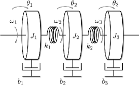
Figure 1: Three inertia system [10]

Example

The proposed Algorithm 1 is implemented for the three-inertia system shown in Figure 1 (considered in [9],[10],[19]) which is 444-sparse observable and has dynamics represented by the following continuous time state space equation:

x˙[t]=˙𝑥delimited-[]𝑡absent\displaystyle\dot{x}[t]= Acx[t]subscript𝐴𝑐𝑥delimited-[]𝑡\displaystyle A_{c}x[t]
y[t]=𝑦delimited-[]𝑡absent\displaystyle y[t]= Ccx[t]+a[t]subscript𝐶𝑐𝑥delimited-[]𝑡𝑎delimited-[]𝑡\displaystyle C_{c}x[t]+a[t] (11)

where

Ac=[010000k1J1b1J1k1J1000000100k1J20k1+k2J2b2J2k2J2000000100k2J30k2J3b2J3]subscript𝐴𝑐delimited-[]010000subscript𝑘1subscript𝐽1subscript𝑏1subscript𝐽1subscript𝑘1subscript𝐽1000000100subscript𝑘1subscript𝐽20subscript𝑘1subscript𝑘2subscript𝐽2subscript𝑏2subscript𝐽2subscript𝑘2subscript𝐽2000000100subscript𝑘2subscript𝐽30subscript𝑘2subscript𝐽3subscript𝑏2subscript𝐽3A_{c}=\left[\begin{array}[]{cccccc}\phantom{-}0&\phantom{-}1&\phantom{-}0&\phantom{-}0&\phantom{-}0&\phantom{-}0\\ -\frac{k_{1}}{J_{1}}&-\frac{b_{1}}{J_{1}}&\frac{k_{1}}{J_{1}}&\phantom{-}0&\phantom{-}0&\phantom{-}0\\ \phantom{-}0&\phantom{-}0&\phantom{-}0&\phantom{-}1&\phantom{-}0&\phantom{-}0\\ \phantom{-}\frac{k_{1}}{J_{2}}&\phantom{-}0&-\frac{k_{1}+k_{2}}{J_{2}}&-\frac{b_{2}}{J_{2}}&\phantom{-}\frac{k_{2}}{J_{2}}&\phantom{-}0\\ \phantom{-}0&\phantom{-}0&\phantom{-}0&\phantom{-}0&\phantom{-}0&\phantom{-}1\\ \phantom{-}0&\phantom{-}0&\phantom{-}\frac{k_{2}}{J_{3}}&\phantom{-}0&-\frac{k_{2}}{J_{3}}&-\frac{b_{2}}{J_{3}}\\ \end{array}\right]
Cc=[100000001000000010101000100010001010]=[C1C2C3]subscript𝐶𝑐delimited-[]100000001000missing-subexpressionmissing-subexpressionmissing-subexpressionmissing-subexpressionmissing-subexpressionmissing-subexpression000010101000missing-subexpressionmissing-subexpressionmissing-subexpressionmissing-subexpressionmissing-subexpressionmissing-subexpression100010001010delimited-[]subscript𝐶1subscript𝐶2subscript𝐶3C_{c}=\left[\begin{array}[]{cccccc}1&0&\phantom{-}0&0&\phantom{-}0&0\\ 0&0&\phantom{-}1&0&\phantom{-}0&0\\ \hline\cr 0&0&\phantom{-}0&0&\phantom{-}1&0\\ 1&0&-1&0&\phantom{-}0&0\\ \hline\cr 1&0&\phantom{-}0&0&-1&0\\ 0&0&\phantom{-}1&0&-1&0\end{array}\right]=\left[\begin{array}[]{c}C_{1}\\ C_{2}\\ C_{3}\end{array}\right]

where J1=0.01kgm2subscript𝐽10.01𝑘𝑔superscript𝑚2J_{1}=0.01\hskip 1.72218ptkgm^{2}, J2=0.02kgm2subscript𝐽20.02𝑘𝑔superscript𝑚2J_{2}=0.02\hskip 1.72218ptkgm^{2}, J3=0.03kgm2subscript𝐽30.03𝑘𝑔superscript𝑚2J_{3}=0.03\hskip 1.72218ptkgm^{2} are the inertias of drive motor, middle body and load respectively, K1=K2=1.4N/radsubscript𝐾1subscript𝐾21.4𝑁𝑟𝑎𝑑K_{1}=K_{2}=1.4\hskip 1.72218ptN/rad are the torsional stiffness of two shafts, B1=B2=B3=0.005N/(rad/s)subscript𝐵1subscript𝐵2subscript𝐵30.005𝑁𝑟𝑎𝑑𝑠B_{1}=B_{2}=B_{3}=0.005\hskip 1.72218ptN/(rad/s) are the mechanical damping of three inertias and x=[θ1,ω1,θ2,ω2,θ3,ω3]𝑥subscript𝜃1subscript𝜔1subscript𝜃2subscript𝜔2subscript𝜃3subscript𝜔3x=[\theta_{1},\omega_{1},\theta_{2},\omega_{2},\theta_{3},\omega_{3}] where θ1,θ2,θ3subscript𝜃1subscript𝜃2subscript𝜃3\theta_{1},\theta_{2},\theta_{3} are the absolute angular positions of three inertias, ω1,ω2,ω3subscript𝜔1subscript𝜔2subscript𝜔3\omega_{1},\omega_{2},\omega_{3} are the speeds of three inertias and the output measurements are the three angular positions and the three relative angular positions. To obtain a discrete-time model, the system in (III-B) is discretized with a sampling period of h=0.1s0.1𝑠h=0.1s. The undirected communication graph of the 3 local observers is connected and the adjacency matrix of this graph is 𝒜=[011100100]𝒜delimited-[]011100100\mathcal{A}=\left[\begin{smallmatrix}0&1&1\\ 1&0&0\\ 1&0&0\end{smallmatrix}\right]. The initial state of the system is taken as x[0]=[0,0,0,0,0.9644,0]T𝑥delimited-[]0superscript00000.96440𝑇x[0]=[0,0,0,0,0.9644,0]^{T}. The third and fourth sensors are attacked and the attack vectors are generated at random. We have τ=3𝜏3\tau=3 measurements collected at t=0,1,2𝑡012t=0,1,2 and the algorithm is initialised at t=3𝑡3t=3. Penalty parameter ρ𝜌\rho is initialised as 1 for all agents and ν,μ1,μ2𝜈subscript𝜇1subscript𝜇2\nu,\mu_{1},\mu_{2} are chosen as 10,2.5102.510,2.5 and 1.11.11.1 respectively. The stopping condition used is a tolerance of 0.1 for the primal and dual residuals.
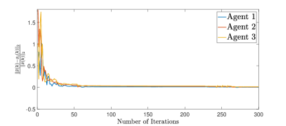
Refer to caption
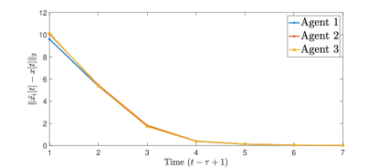
Figure 2: Evolution of the consensus error in the state estimates of all local observers across time
Refer to caption
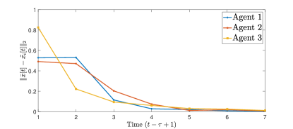
Figure 3: Evolution of error in the state estimate of all agents across time

The comparison of consensus error associated with all the local observers is shown in Figure 2 and the evolution of error in state estimate of all the observers across time is shown in Figure 3. In this case, the average number of inner loop iterations the observer algorithm takes in a time step is 40.

We next adapt Algorithm 1 for the DSSE problem and the design of a centralized observer with sensor attacks and compare the performance with the existing algorithms in literature.

III-B1 Case 1 - Implementation as Distributed Secure State Estimator

Algorithm 1 is modified to address the DSSE problem by executing the inner loop alone with loop guard as rikαsuperscriptsubscript𝑟𝑖𝑘𝛼r_{i}^{k}\leq\alpha, sikβsuperscriptsubscript𝑠𝑖𝑘𝛽s_{i}^{k}\leq\beta, for some small α,β𝛼𝛽\alpha,\beta, instead of rit(1ν)rit1superscriptsubscript𝑟𝑖𝑡1𝜈superscriptsubscript𝑟𝑖𝑡1r_{i}^{t}\leq(1-\nu)r_{i}^{t-1}, sit(1ν)sit1superscriptsubscript𝑠𝑖𝑡1𝜈superscriptsubscript𝑠𝑖𝑡1s_{i}^{t}\leq(1-\nu)s_{i}^{t-1} to solve the optimization problem given in (10) i.e. to estimate the initial state x[t0]𝑥delimited-[]subscript𝑡0x[t_{0}] using a batch of measurements collected from time t=t0𝑡subscript𝑡0t=t_{0} to t=t0+τ1𝑡subscript𝑡0𝜏1t=t_{0}+\tau-1.

Refer to caption
Figure 4: Evolution of consensus error in the agent state estimates in case of implementation as Distributed Secure State Estimator
Refer to caption
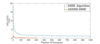
Figure 5: Comparison of the error in state estimate of agent 2

This idea is implemented and compared with the DSSE algorithm in [10] for the system considered earlier. Since the DSSE algorithm assumes a sparse initial state, the initial state for the system is taken as x[0]=[0,0.7196,0,0,0,0]T𝑥delimited-[]0superscript00.71960000𝑇x[0]=[0,0.7196,0,0,0,0]^{T} and the third and sixth sensors are attacked. Penalty parameter ρ𝜌\rho is initialised as 1 for all agents and ν,μ1,μ2𝜈subscript𝜇1subscript𝜇2\nu,\mu_{1},\mu_{2} are chosen as 10,2,2102210,2,2 respectively. Both the algorithms are run for 1000 iterations. Figure 4 shows the comparison of consensus error associated with all the agents for our ADMM-based algorithm and Figure 5 shows the error in state estimate of agent 2 for both the algorithms. We observe that our algorithm converges faster.

III-B2 Case 2 - Implementation as Centralized Observer

Since centralized observer under sparse sensor attacks exists in literature, we adapt our distributed observer in Algorithm 1 for the centralized case and compare its performance with the ETPL observer in [5].

Algorithm 2 ADMM based Centralized Observer
1:  Initialize τ>0𝜏0\tau>0 and collect measurements from time t0subscript𝑡0t_{0} to t0+τ1subscript𝑡0𝜏1t_{0}+\tau-1
2:  Initialize t=t0+τ𝑡subscript𝑡0𝜏t=t_{0}+\tau, λ0,ρ>0,rt1formulae-sequencesuperscript𝜆0𝜌0superscript𝑟𝑡1\lambda^{0},\rho>0,r^{t-1} and z~(t1)~𝑧𝑡1\tilde{z}(t-1)
3:  while rt1αsuperscript𝑟𝑡1𝛼r^{t-1}\geq\alpha do
4:     Time Update:z~T(t)=A¯z~(t1)+Ny(t)subscript~𝑧𝑇𝑡¯𝐴~𝑧𝑡1𝑁𝑦𝑡\hskip 4.30554pt\tilde{z}_{T}(t)=\bar{A}\tilde{z}(t-1)+{N}{y}(t)
5:     Initialize k=1𝑘1k=1, rt=rt1superscript𝑟𝑡superscript𝑟𝑡1r^{t}=r^{t-1}
6:     while rt(1ν)rt1superscript𝑟𝑡1𝜈superscript𝑟𝑡1r^{t}\geq(1-\nu)r^{t-1} do
7:        z~k=argminz~=(x~,E~)E~1+(λk1)T(Qz~Y¯)+ρ2Qz~Y¯22superscript~𝑧𝑘~𝑧~𝑥~𝐸subscriptnorm~𝐸1superscriptsuperscript𝜆𝑘1𝑇𝑄~𝑧¯𝑌𝜌2superscriptsubscriptnorm𝑄~𝑧¯𝑌22\tilde{z}^{k}=\underset{\tilde{z}=(\tilde{x},\tilde{E})}{\arg\min}\|\tilde{E}\|_{1}+(\lambda^{k-1})^{T}(Q\tilde{z}-\bar{Y})+\frac{\rho}{2}\|Q\tilde{z}-\bar{Y}\|_{2}^{2}
8:        λk=λk1+ρ(Qz~kY¯)superscript𝜆𝑘superscript𝜆𝑘1𝜌𝑄superscript~𝑧𝑘¯𝑌\lambda^{k}=\lambda^{k-1}+\rho(Q\tilde{z}^{k}-\bar{Y})
9:        rt=Qz~kY¯2superscript𝑟𝑡subscriptnorm𝑄superscript~𝑧𝑘¯𝑌2r^{t}=\|Q\tilde{z}^{k}-\bar{Y}\|_{2}
10:        k=k+1𝑘𝑘1k=k+1
11:     end while
12:     z~(t)=z~k1,λ0=λk1formulae-sequence~𝑧𝑡superscript~𝑧𝑘1superscript𝜆0superscript𝜆𝑘1\tilde{z}(t)=\tilde{z}^{k-1},\lambda^{0}=\lambda^{k-1}
13:     t=t+1𝑡𝑡1t=t+1
14:  end while

This is given as Algorithm 2.

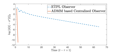
We consider the system in (III-B) with initial state x[0]=[0.5453,0.6888,0.1474,0.7776,0.3991,0.8983]T𝑥delimited-[]0superscript0.54530.68880.14740.77760.39910.8983𝑇x[0]=[0.5453,0.6888,0.1474,0.7776,0.3991,0.8983]^{T}. The third and fourth sensors are attacked. Penalty parameter ρ𝜌\rho is chosen as 1 for Algorithm 2. Figure 6 shows the evolution of the error in state estimate for both the algorithms. It can be observed that our algorithm converges significantly faster.
Refer to caption
Figure 6: Comparison of the evolution of error (in logarithmic scale) in the system state estimate of both the algorithms. The stopping condition used is a tolerance of 105superscript10510^{-5} for the primal residual.

IV Conclusion

In this paper, we addressed the problem of designing a distributed observer for the state estimation of a discrete time LTI system under sparse sensor attack. An algorithm based on ADMM was proposed, for the update of each local observer, by which a network of observers were able to asymptotically estimate the system state using each of their limited, corrupt measurements and by communication with their neighbours. The proposed algorithm was adapted to solve the DSSE problem and also design a centralized observer. The performance was compared with other algorithms in literature for a well-studied system. As future work, adoption of event triggering techniques to reduce the number of communications among agents and distributed observer design under attack for directed networks could be of interest.

References

  • [1] A. A. Cárdenas, S. Amin, and S. Sastry, “Research challenges for the security of control systems,” in Proceedings of the 3rd Conference on Hot Topics in Security, ser. HOTSEC’08.   USA: USENIX Association, 2008.
  • [2] M. J. Khojasteh, A. Khina, M. Franceschetti, and T. Javidi, “Learning-based attacks in cyber-physical systems,” IEEE Transactions on Control of Network Systems, 09 2020.
  • [3] T. Pultarova, “Cyber security - ukraine grid hack is wake-up call for network operators [news briefing],” Engineering & Technology, vol. 11, no. 1, pp. 12–13, 2016.
  • [4] W. Duo, M. Zhou, and A. Abusorrah, “A survey of cyber attacks on cyber physical systems: Recent advances and challenges,” IEEE/CAA Journal of Automatica Sinica, vol. 9, no. 5, pp. 784–800, 2022.
  • [5] Y. Shoukry and P. Tabuada, “Event-triggered state observers for sparse sensor noise/attacks,” IEEE Transactions on Automatic Control, vol. 61, no. 8, pp. 2079–2091, 2016.
  • [6] A.-Y. Lu and G.-H. Yang, “Secure luenberger-like observers for cyber–physical systems under sparse actuator and sensor attacks,” Automatica, vol. 98, pp. 124–129, 2018.
  • [7] A. Mitra and S. Sundaram, “Distributed observers for lti systems,” IEEE Transactions on Automatic Control, vol. 63, no. 11, pp. 3689–3704, 2018.
  • [8] W. Han, H. L. Trentelman, Z. Wang, and Y. Shen, “A simple approach to distributed observer design for linear systems,” IEEE Transactions on Automatic Control, vol. 64, no. 1, pp. 329–336, 2019.
  • [9] L. An and G.-H. Yang, “Distributed secure state estimation for cyber–physical systems under sensor attacks,” Automatica, vol. 107, pp. 526–538, 2019.
  • [10] T. Shinohara and T. Namerikawa, “Distributed secure state estimation with a priori sparsity information,” IET Control Theory and Applications, vol. 16, no. 11, pp. 1086–1097, Jul. 2022.
  • [11] W. Ao, Y. Song, and C. Wen, “Distributed secure state estimation and control for cpss under sensor attacks,” IEEE Transactions on Cybernetics, vol. 50, no. 1, pp. 259–269, 2020.
  • [12] A. Mitra and S. Sundaram, “Byzantine-resilient distributed observers for lti systems,” Autom., vol. 108, 2019.
  • [13] J. Kim, J. G. Lee, C. Lee, H. Shim, and J. H. Seo, “Local identification of sensor attack and distributed resilient state estimation for linear systems,” in 2018 IEEE Conference on Decision and Control (CDC), 2018, pp. 2056–2061.
  • [14] H. Fawzi, P. Tabuada, and S. Diggavi, “Secure state-estimation for dynamical systems under active adversaries,” in 2011 49th Annual Allerton Conference on Communication, Control, and Computing (Allerton), 2011, pp. 337–344.
  • [15] T. Shinohara, T. Namerikawa, and Z. Qu, “Resilient reinforcement in secure state estimation against sensor attacks with a priori information,” IEEE Transactions on Automatic Control, vol. 64, no. 12, pp. 5024–5038, 2019.
  • [16] H. Paul, J. Fliege, and A. Dekorsy, “In-network-processing: Distributed consensus-based linear estimation,” IEEE Communications Letters, vol. 17, no. 1, pp. 59–62, 2013.
  • [17] S. Boyd, N. Parikh, E. Chu, B. Peleato, J. Eckstein et al., “Distributed optimization and statistical learning via the alternating direction method of multipliers,” Foundations and Trends® in Machine learning, vol. 3, no. 1, pp. 1–122, 2011.
  • [18] G. Notarstefano, I. Notarnicola, and A. Camisa, Distributed Optimization for Smart Cyber-Physical Networks, 2019.
  • [19] G. Zhang and J. Furusho, “Vibration control of three-inertia system,” in IECON Proceedings (Industrial Electronics Conference), vol. 3, 1999, pp. 1045–1050.