Universal measurement-based quantum computation in a one-dimensional architecture
enabled by dual-unitary circuits

Abstract

A powerful tool emerging from the study of many-body quantum dynamics is that of dual-unitary circuits, which are unitary even when read ‘sideways’, i.e., along the spatial direction. Here, we show that this provides the ideal framework to understand and expand on the notion of measurement-based quantum computation (MBQC). In particular, applying a dual-unitary circuit to a many-body state followed by appropriate measurements effectively implements quantum computation in the spatial direction. We argue that this computation can be made deterministic by enforcing a Clifford condition, and is generically universal. Remarkably, all these requirements can already be satisfied by the dynamics of the paradigmatic kicked Ising chain at specific parameter choices. Specifically, after $k$ time-steps, equivalent to a depth-$k$ quantum circuit, we obtain a resource state for universal MBQC on $\sim 3k/4$ encoded logical qubits. This removes the usual requirement of going to two dimensions to achieve universality, thereby reducing the demands imposed on potential experimental platforms. Beyond the practical advantages, we also interpret this evolution as an infinite-order entangler for symmetry-protected topological chains, which gives a vast generalization of the celebrated cluster chain and shows that our protocol is robust to symmetry-respecting deformations.

Introduction.—Recent years have seen significant advances at the frontier of many-body quantum dynamics. A particularly fruitful approach has been to study time-evolution induced by quantum circuits, minimal models of dynamics in which degrees of freedom are updated by local unitary gates. Imposing structure on these gates lead to different classes of dynamics —including Clifford Gottesman (1997), matchgate Valiant (2002); Terhal and DiVincenzo (2002); Jozsa and Miyake (2008), and Haar random circuits Nahum et al. (2017, 2018); Khemani et al. (2018); Rakovszky et al. (2018); Sünderhauf et al. (2018); Chan et al. (2018); von Keyserlingk et al. (2018); Fisher et al. (2022)—which allow for the the efficient computation of physical quantities while still capturing different interesting regimes of behavior. A recent promising class is that of dual-unitary circuits Bertini et al. (2019); Akila et al. (2016); Gopalakrishnan and Lamacraft (2019); Bertini and Piroli (2020); Piroli et al. (2020); Suzuki et al. (2022); Kos et al. (2021); Claeys and Lamacraft (2021); Zhou and Harrow (2022), which are composed of gates that are not only unitary in the time-direction, as required by dynamics in closed quantum systems, but also unitary in the space-direction, upon exchanging the role of space and time. Despite this strong property, the class of dual-unitaries is broad and rich, capturing both integrable and chaotic systems Bertini et al. (2019); Claeys and Lamacraft (2021). The versatility of this approach has seen many applications, allowing one to exactly compute spatio-temporal correlation functions Bertini et al. (2019); Claeys and Lamacraft (2021), spectral statistics Bertini et al. (2018, 2021), and entanglement dynamics Piroli et al. (2020); Reid and Bertini (2021), thereby providing deep insights into phenomena like quantum chaos, information scrambling and thermalization.

Intriguingly, the idea of regarding one spatial direction as an effective time-direction along which a circuit runs appears already in an older topic, namely that of measurement-based quantum computation (MBQC) Raussendorf et al. (2003); Raussendorf and Wei (2012). Here, the idea is that by creating an entangled many-body ‘resource’ state using a finite-depth circuit and subsequently measuring the qubits, it is possible to effectively propagate quantum information through the spatial direction. The desired class of resource states is such that this spatial propagation is, indeed, unitary. Remarkably, there exist resource states in two spatial dimensions (2D) which are universal, meaning that this unitary evolution in the spatial direction can efficiently realize any quantum operation acting on any given number of encoded qubits Raussendorf and Briegel (2001). Decades of research has uncovered a plethora of such universal resources Gross and Eisert (2007); Brennen and Miyake (2008); Kwek et al. (2012); Wei (2018); Gachechiladze et al. (2019), including a fault-tolerant protocol in 3D Raussendorf et al. (2006), but the full classification of universal resource states is still ongoing Prakash and Wei (2015); Wang et al. (2017); Stephen et al. (2017); Miller and Miyake (2018); Stephen et al. (2019); Daniel et al. (2020); Herringer and Raussendorf (2022). Both computation and fault-tolerance in MBQC have been realized in proof-of-principle experiments Walther et al. (2005); Prevedel et al. (2007); Yao et al. (2012).

Here, we show how insights from dual-unitarity can shed new light on MBQC, both at a conceptual and practical level. Namely, reading a dual-unitary circuit in the time direction describes the preparation of the resource state, while reading it in the spatial direction directly reveals the logical circuit induced by appropriate measurement of the resource state, as pictured in Fig. 1. This provides an accessible alternative approach to MBQC beyond the traditional stabilizer Raussendorf et al. (2003), teleportation Childs et al. (2005), or matrix product state-based  Gross and Eisert (2007) formalisms, and highlights how resource states can emerge naturally under certain classes of quantum many-body dynamics. These results also elevate dual-unitarity from an abstract computational tool to a concept with direct practical application.

Figure 1: Graphical depiction of Eq. 4 for $k=N=4$. The red (blue) rounded box indicates one application of $T_{N}$ ($T_{k}$). In accordance with the convention of quantum circuits, the order of matrix multiplication in the right figure is from left to right.

While Refs. Ho and Choi, 2022; Claeys and Lamacraft, 2022; Ippoliti and Ho, 2022 explored how measurements can stochastically induce a universal gateset in the spatial direction of such circuits, performing scalable quantum computation requires deterministic control without post-selection of measurement outcomes. In this paper, we show that, by using dual-unitary circuits which are additionally chosen to be Clifford, it is possible to implement deterministic MBQC without sacrificing universality. Specifically, we show that a depth-$k$ dual-unitary circuit composed of repeated applications of uniform single-site and nearest-neighbour Ising entangling gates on a chain prepares a resource state for MBQC on $k$ encoded qubits. We then identify an unbounded sequence of $k$ for which the resulting unitary evolution that can be efficiently implemented via measurement is universal on at least $\sim 3k/4$ of the encoded qubits. The key practical advantage of our protocol is the removal of the need to go to 2D geometries for universal MBQC while still only requiring simple and uniform controls (as compared to, e.g., embedding a universal 2D state in 1D with a linear-depth circuit Suzuki et al. (2022)). This shortens the list of requirements for potential implementation in experimental platforms, and is particularly relevant to trapped ions Bruzewicz et al. (2019); Monroe et al. (2021), which harbor among the highest gate and measurement fidelities, and also the long coherence times required for the crucial feedforward technology Barrett et al. (2004); Chiaverini et al. (2004); Riebe et al. (2008); Ryan-Anderson et al. (2021), yet are typically restricted to a 1D geometry.

From another perspective, the dual-unitary circuits we consider can be viewed as “infinite-order” entanglers for symmetry-protected topological (SPT) orders Chen et al. (2013). That is, after $k$ time steps, the resulting state possesses 1D SPT order with complexity that increases unboundedly with $k$, as quantified by, e.g., the size of the degenerate edge modes. On one hand, this shows that certain dual-unitary circuits provide a new way to generate infinite families of SPT order, which have proven very useful to the study of SPT order in the past Fidkowski and Kitaev (2011); Lahtinen and Ardonne (2015); Verresen et al. (2017, 2018); Jones and Verresen (2019); Jones et al. (2021); Jones and Verresen (2021); Balabanov et al. (2021, 2022). On the other hand, this insight connects our results to the large literature on using SPT phases as resources for MBQC Prakash and Wei (2015); Wang et al. (2017); Stephen et al. (2017); Miller and Miyake (2018); Stephen et al. (2019); Daniel et al. (2020); Doherty and Bartlett (2009); Bartlett et al. (2010); Miyake (2010); Else et al. (2012a); Miller and Miyake (2015); Poulsen Nautrup and Wei (2015); Miller and Miyake (2016); Wei and Huang (2017); Raussendorf et al. (2019); Devakul and Williamson (2018). In particular, it allows us to directly apply previous results Else et al. (2012a); Stephen et al. (2017, 2019) to show that our MBQC schemes work not only using the fixed-point states generated by the dual-unitary evolution, but also any generic deformations thereof preserving certain symmetries.

Resource states from a dual-unitary circuit.— We consider $N$ qubits arranged on a line, denote Pauli operators as $X,Y,Z$, and write the eigenbasis of $Z$ as $|0\rangle,|1\rangle$. Dynamics are generated by the kicked Ising model, which is defined by the Floquet evolution $U_{F}=e^{-ih\sum_{i=1}^{N}Y_{i}}e^{-iH_{\text{Ising}}\tau}$ where $H_{\text{Ising}}=J\sum_{i=1}^{N-1}Z_{i}Z_{i+1}+g\sum_{i=1}^{N}Z_{i}$. We fix $\tau=1$ and $J,h=\pm\pi/4$, since the evolution generated by $U_{F}$ is dual unitary only for these parameters. The parameter $g$ is chosen such that the evolution is also Clifford, meaning that any product of Pauli operators is mapped to another product of Pauli operators under conjugation by $U_{F}$. This important property will allow us compensate for random measurement outcomes and achieve deterministic computation. This property holds for $g=0$ and $g=\pm\pi/4$, but we focus on the latter as the former corresponds to free-fermion evolution which generates efficiently simulable matchgate circuits and thus inhibits universal MBQC (see Appendix E). $U_{F}$ is then equivalent to the following quantum circuit (up to irrelevant phases and Pauli operators ):

$$T_{N}=\prod_{i=1}^{N}H_{i}S_{i}\prod_{i=1}^{N-1}CZ_{i,i+1},$$ (1)

where we define the gates $CZ=I-2|11\rangle\langle 11|$, $H=\frac{X+Z}{\sqrt{2}}$ and $S=\sqrt{Z}=\mathrm{diag}(1,i)$. We note that the single-qubit gate $HS$ cyclically permutes the three Pauli operators under conjugation.

The resource states $|\psi_{k}\rangle$ are defined by acting on an initial product state with the unitary circuit (or equivalently Floquet unitary) $k$ times,

$$|\psi_{k}\rangle=T_{N}^{k}\left(\bigotimes_{i=1}^{N}|+\rangle_{i}\right),$$ (2)

where $|\pm\rangle=\frac{|0\rangle\pm|1\rangle}{\sqrt{2}}$. These states are pictured in Fig. 1. Since $T_{N}$ is a Clifford circuit, the states $|\psi_{k}\rangle$ are stabilizers states that are uniquely defined by the equations $S^{(k)}_{i}|\psi_{k}\rangle=|\psi_{k}\rangle$, where

$$S^{(k)}_{i}=T_{N}^{k}X_{i}T_{N}^{k\dagger}.$$ (3)

Equivalently, $|\psi_{k}\rangle$ is the unique ground state of the gapped Hamiltonian $H_{k}=-\sum_{i}S^{(k)}_{i}$. For example, we have $S^{(1)}_{i}=X_{i-1}Y_{i}X_{i+1}$ (with modifications near the ends of the chain), so $|\psi_{1}\rangle$ is the 1D cluster state Raussendorf et al. (2003). The 1D cluster state is a prototypical resource for MQBC on a single encoded qubit, and also a simple example of 1D SPT order Son et al. (2012). We will show that, as $k$ is increased, the states $|\psi_{k}\rangle$ are resources for MBQC on $k$ encoded qubits, and have 1D SPT order with respect to a symmetry group that grows with $k$.

Now we will describe a protocol for MBQC using the states $|\psi_{k}\rangle$ as resource states. The equivalence of our measurement-based scheme to the traditional unitary gate-based model will follow directly from the dual-unitarity of $T_{N}^{k}$. In our protocol, each qubit in the chain is measured sequentially from left to right in a rotated basis in the $YZ$-plane, i.e., in a basis $\{|0^{\theta}\rangle,|1^{\theta}\rangle\}$ defined by an angle $\theta$ where $|s^{\theta}\rangle=e^{-i\theta X}|s\rangle$. The output of the quantum computation is determined by the probabilities of obtaining different measurement outcomes, which, according to the Born rule, are given by the inner products $|\langle s_{1}^{\theta_{1}},\dots,s_{N}^{\theta_{N}}|\psi_{k}\rangle|^{2}$ where each $s_{i}=0,1$. To determine these overlaps, we utilize the dual-unitary property of the circuit $T_{N}^{k}$. Namely, as shown in Fig. 1, we can read the circuit “sideways” to find,

$$\langle s_{1}^{\theta_{1}},\dots,s_{N}^{\theta_{N}}|\psi_{k}\rangle=\langle R|U(\theta_{N},s_{N})\dots U(\theta_{1},s_{1})|L\rangle$$ (4)

where we have defined the vectors $|L\rangle=\bigotimes_{i=1}^{k}|+\rangle_{i}$ and $|R\rangle=\bigotimes_{i=1}^{k}|0\rangle_{i}$ and the unitary operator $U(\theta,s)=T_{k}e^{i\theta Z_{1}}Z_{1}^{s}$ where $T_{k}$ is as defined in Eq. 1. This equivalence is demonstrated in greater detail in Appendix A. We see that, due to the dual-unitarity of $T_{N}^{k}$, the calculation of the inner product coming from the Born rule is equivalent to the output of a quantum computation occurring in a “virtual” Hilbert space consisting of $k$ qubits. The virtual qubits are initialized in a state $|L\rangle$, evolved by unitaries $U(\theta,s)$, and the projected onto a final state $|R\rangle$. The evolution during this process depends on the measurement bases defined by the angles $\theta_{i}$. Therefore, by choosing our measurement bases, we can enact different unitary evolutions on the virtual qubits. Thus, the dual-unitarity of the circuit representing the dynamics provides a natural perspective on how measurement of physical qubits translates into controllable unitary evolution of encoded qubits .

Currently, the evolution of the virtual qubits depends not only on the angles $\theta_{i}$ but also the measurement outcomes $s_{i}$, which are random. However, owing importantly to the Clifford nature of dynamics of $T_{k}$, this randomness can be straightforwardly accounted for by adjusting future measurement bases depending on past measurement outcomes (as is common to all schemes of MBQC), such that the overall evolution is deterministic. We describe this in detail in Appendix B, and for the rest of the main text we always assume the outcome $|0^{\theta}\rangle$ is obtained. In short, the effect of obtaining the “wrong” measurement outcome $|1^{\theta}\rangle$ is to insert the byproduct operator $Z_{1}$ at that step in the computation. To deal with this unwanted operator, we imagine pushing it through to the end of the circuit. Because $T_{k}$ is Clifford, $Z_{1}$ will remain a product of Pauli operators as it is pushed through each layer of the circuit, which therefore only has two controlled effects: First, depending on where the wrong outcome occurred, a subset of the rotation angles at later times will be flipped, $\theta_{i}\rightarrow-\theta_{i}$. This can be counteracted by flipping $\theta_{i}$ in the corresponding bases of future measurements. Second, once the byproduct operator is pushed to the end, it acts on $|R\rangle$ in such a way that $|R\rangle$ gets mapped onto a random product state in the $|0/1\rangle$-basis depending on the complete history of all measurement outcomes. Therefore, when accounting for the random measurement outcomes, repeating the protocol many times while recording the measurement statistics $|\langle s_{1}^{\theta_{1}},\dots,s_{N}^{\theta_{N}}|\psi_{k}\rangle|^{2}$ allows us to garner the measurement statistics $|\langle i_{1},\dots,i_{k}|\phi_{\mathrm{out}}\rangle|^{2}$ for all $|i_{j}\rangle=|0/1\rangle$ where $|\phi_{\mathrm{out}}\rangle=U(\theta_{N})\dots U(\theta_{1})|L\rangle$ with $U(\theta_{i})=T_{k}e^{i\theta_{i}Z_{1}}$ is the output state of the virtual computation. This constitutes a complete scheme of quantum computation, where we initialize a quantum register in a known state $|L\rangle$, perform deterministic unitary evolution on it, and read-out the final output state in a fixed basis.

Determining the set of gates.—What remains is to determine which unitary circuits can be implemented using products of the unitaries $U(\theta)$. To understand these circuits, we make the important observation that, since $T_{k}$ is unitary and Clifford, it has a finite period, meaning there is a smallest integer $p_{k}$ such that $T_{k}^{p_{k}}\propto I$. Now, consider breaking the computation into blocks of length $p_{k}$. The net effect of measuring all spins in one block is

$$\prod_{\ell=0}^{p_{k}-1}U(\theta_{\ell})=\prod_{\ell=0}^{p_{k}-1}T_{k}e^{i\theta_{\ell}Z_{1}}\propto\prod_{\ell=0}^{p_{k}-1}e^{i\theta_{\ell}O_{k}(\ell)},$$ (5)

where $O_{k}(\ell):=T_{k}^{\ell\dagger}Z_{1}T_{k}^{\ell}$. Therefore, the elementary gates in our scheme are $k$-qubit rotations generated by the operators $O_{k}(\ell)$, which are determined by the space-time evolution of $Z_{1}$ under conjugation by $T_{k}^{\dagger}$ a number $\ell$ times. Again, as $T_{k}$ is a Clifford circuit, these operators will all be $k$-qubit Pauli operators. The evolution is determined (up to a possible factor of $-1$) from the following local rules,

$$T_{k}^{\dagger}X_{i}T_{k}=Z_{i},\ T_{k}^{\dagger}Z_{i}T_{k}=\begin{cases}Y_{1}Z_{2}&i=1\\ Z_{i-1}Y_{i}Z_{i+1}&1<i<k\\ Z_{k-1}Y_{k}&i=k\end{cases}$$ (6)

The space-time evolution of Pauli operators starting with $Z_{1}$ subject to these rules generates a fractal pattern that is pictured in Fig. 2. Let $\mathcal{O}_{k}$ denote the set of all $O_{k}(\ell)$ for $\ell=0,\dots,p_{k}-1$. For a small angle $d\theta$, we have $e^{d\theta A}e^{d\theta B}e^{-d\theta A}e^{-d\theta B}\approx e^{(d\theta)^{2}[A,B]}$ where $[A,B]=AB-BA$ for $A,B\in\mathcal{O}_{k}$. Using this, we can perform any rotation of the form $R=e^{iA}$ where $A$ is an element of the Lie algebra $\mathcal{A}_{k}$ obtained by closing the set $\mathcal{O}_{k}$ under commutation. The set of such rotations is our set of implementable unitaries.

$k$	1	2	3	4	5	6	7
$p_{k}$	3	4	12	10	24	18	24
dim($\mathcal{A}_{k}$)	3	10	63	120	496	4095	8256
$\mathcal{A}_{k}$	$su(2^{k})$	$sp(2^{k})$	$su(2^{k})$	$so(2^{k})$	$so(2^{k})$	$su(2^{k})$	$sp(2^{k})$

Figure 2: Top: Depiction of the operators $O_{k}(\ell)$ up to a phase for $k=7,31$ with respective periods $p_{k}=24,96$. Each column indexed by $\ell$ represents one product of Pauli operators acting on the $k$ logical qubits which are indexed by $i=1,\dots,k$. The operator in one column is obtained from the previous via the local rules in Eq. 6. The solid and dashed red boxes indicate repeating structures used in the proof of computational universality. The string of $I$ and $Z$ at the top indicates the repeating pattern found in the symmetry of $|\psi_{k}\rangle$ for $k=7$, where $Z$ operators appear whenever there is an $X$ or $Y$ operator in the top row of the space-time operator evolution. Bottom: Numerically determined computational power for small $k$. The lower row lists Lie algebras with dimensions consistent with the numerical calculations, where $su(n)$, $so(n)$, and $sp(n)$ denote the algebras of special unitary, orthogonal, and symplectic matrices.

To determine this set, we must determine the Lie algebra $\mathcal{A}_{k}$. Ideally, we desire $\mathcal{A}_{k}=su(2^{k})$, i.e., $\mathcal{A}_{k}$ contains all $2^{2k}-1$ Pauli operators acting on $k$ qubits, which gives universal computation on all $k$ qubits. At first glance, this seems impossible, since the only operations we use are $Z$ rotations of the first qubit and the application of a fixed $T_{k}$ to all qubits, so it is not clear how to selectively control a generic target qubit. However, we find that the persistent application of $T_{k}$ allows us to convert temporal control into spatial control. A similar concept was used in Ref. Raussendorf, 2005. Indeed, looking at Fig. 2, we see that each operator $O_{k}(\ell)$ acts differently on different qubits. By judiciously combining these operators, we can selectively control other qubits.

As a first investigation into the form of $\mathcal{A}_{k}$, we numerically generate the operators in $\mathcal{O}_{k}$ for small $k$ and repeatedly take commutators until no new operators are found. Then, we look at the size of the resulting algebra and identify it with known Lie algebras. This is shown in Fig. 2 for $k\leq 7$. We see that, in each case, we get an algebra with a dimension that scales exponentially with the number of qubits, but we only get the full $su(2^{k})$ in certain cases. While the full algebra $\mathcal{A}_{k}$ appears to depend on $k$ in a complicated manner, we are able to prove the following result:

Theorem 1.

For every $k\geq 3$, let $m=\lfloor\frac{k+1}{4}\rfloor$. Then, the set of gates implementable in MBQC using the state $|\psi_{k}\rangle$ as a resource is universal on at least $3m$ qubits. That is, $su(2^{3m})\subset\mathcal{A}_{k}$. If we further have $k=2^{r}-1$ for some $r\geq 0$, then all elementary gates are guaranteed to be implemented with at most a linear overhead in $k$.

Therein, $\lfloor x\rfloor$ denotes the largest integer less than or equal to $x$. This is the main result of this work, as it means that the resource states $|\psi_{k}\rangle$ can be used for universal MBQC on $\sim 3k/4$ qubits. The proof of this result, given in Appendix C, uses the self-similar fractal nature of the space-time operator evolution depicted in Fig. 2. Namely, we make use of repeating structures in this evolution to extend results for small values of $k$, which we have established numerically, to arbitrarily large values of $k$. For the second part of the Theorem, we show that the period $p_{k}$—which essentially sets a clock speed for our computation since each elementary gate $e^{i\theta O_{k}(\ell)}$ can only be applied once per period—is linear in $k$ when $k=2^{r}-1$. We note that this Theorem is a lower bound on the computational power, meaning that the full gate set will in general be larger than what is given by the Theorem, as can be seen in the table in Fig. 2. Similarly, for $k\neq 2^{r}-1$, the period may be exponentially large in $k$. This puts a large overhead on our clock speed, but at the same time it extends our set of elementary gates $e^{i\theta O_{k}(\ell)}$, meaning we need to spend fewer resources generating higher-order commutators of the $O_{k}(\ell)$ to get arbitrary unitaries. Overall, beyond the minimal results guaranteed by our Theorem, the performance of the states $|\psi_{k}\rangle$ as MBQC resources will depend heavily on both $k$ and the quantum circuit one aims to simulate.

Computational phases of matter.—We have described a universal scheme of MBQC using the states $|\psi_{k}\rangle$ as resource states. It turns out that these states can also be interpreted as fixed-point states of certain 1D symmetry-protected topological (SPT) phases of matter, and that our MBQC scheme can be extended beyond fixed-point states of these phases. To describe the SPT order, we first need to identify the symmetries. For this, we notice that Eq. (4) essentially defines a matrix product state (MPS) representation of the wavefunction Cirac et al. (2021), from which the symmetries can straightforwardly determined (see Appendix D). From this analysis, we find that the symmetries each form a pattern of $Z$ and $I$ operators that repeat across the chain with a unit cell of size $p_{k}$. For example, the state $|{\psi}_{k=1}\rangle$ has symmetry $ZZIZZI\dots$ that repeats with a unit cell of size $p_{1}=3$. This operator and its translations generate a $\mathbb{Z}_{2}\times\mathbb{Z}_{2}$ symmetry. While this is distinct from the usual symmetry operators which one associates to the cluster chain Son et al. (2012), these generalized “cyclic” symmetries in 1D systems have been studied in Refs. Stephen et al., 2019; Sauerwein et al., 2019. The repeating pattern reflects the underlying space-time evolution of the operators $O_{k}(\ell)$, such that the symmetries are also deeply linked to the dual-unitary structure. More precisely, the symmetry group of $|\psi_{k}\rangle$ is generated by (translated versions of) an operator $u=\prod_{i=1}^{N}Z_{i}^{c_{i}}$ where $c_{i}=1$ if $T_{k}^{i\dagger}Z_{1}T_{k}^{i}$ acts as $X$ or $Y$ on the first logical qubit, and $c_{i}=0$ otherwise . That is, the symmetry follows the pattern of the first row of the space-time evolution of the operators $O_{k}(\ell)$, see Fig. 2 for the case $k=7$. The full symmetry group generated by $u$ and its translations is isomorphic to $\mathbb{Z}_{2}^{2k}$ (Appendix D).

The same MPS analysis also reveals the nature of the SPT order of the state $|\psi_{k}\rangle$ under the $\mathbb{Z}_{2}^{2k}$ symmetry. We find that the SPT order is “maximally non-trivial”, meaning that the protected zero-energy edge mode that is characteristic of the SPT order has dimension $2^{k}$, which is the maximal possible value for this symmetry group. Therefore, the complexity of the SPT order, measured by this degeneracy, grows exponentially with $k$. Because of this, the general results of Refs. Else et al., 2012a; Stephen et al., 2017, 2019 can be directly applied to our context to show that the MBQC protocol we have developed for the fixed-point states $|\psi_{k}\rangle$ works, with some modification, for any resource state coming from the same SPT phase. That is, given a state that is promised to be in the same SPT phase as one of our resource states, we can use that state to perform the same set of universal gates using only single-site measurements, even without knowing the microscopic details of the state beforehand. Therefore, the ability to perform universal MBQC is a property not only of the fine-tuned states $|\psi_{k}\rangle$, but also of the entire phases of matter in which they reside.

Discussion.—We have defined a protocol, enabled by dual-unitarity, to generate universal resource states for MBQC in a one-dimensional architecture using single-qubit gates and Ising interactions applied in a uniform fashion. We conclude with a discussion of some interesting features of our protocol. Our elementary gate set implemented by MBQC differs from the usual set of single-qubit rotations and nearest-neighbour two-qubit gates. In particular, entangling operations on a large fraction of the $k$ qubits can be performed in a single time step. Practically, this could lead to large savings in circuit depth for certain algorithms, as was the case in Ref. Gachechiladze et al., 2019 which used a different alternative resource state. This motivates searching for problems that are naturally suited to our gate set, and also for efficient ways to compile more common gate sets into ours, where the methods of Ref. Chen et al., 2022 should be particularly useful.

From a fundamental standpoint, our results show that the dual unitary circuit $T_{N}^{k}$ can also be interpreted as an “infinite-order” SPT entangler. Namely, consecutive applications of $T_{N}$ to an initial product state generates an infinite sequence of more and more complex 1D SPT orders when $N\rightarrow\infty$. This is in contrast to previously-studied SPT entanglers which have finite order, meaning the sequence of SPT orders repeats with finite period as a consequence of the fact that the set of SPT phases with a given symmetry group forms a finite group Chen et al. (2013). Our construction gets around this by virtue of the fact that the symmetry group also grows at each step. This suggests the existence of a relationship between dual-unitary circuits, infinite-order SPT entanglers, and resource states for MBQC. We give a second example of this relationship in Appendix E, which is defined by a circuit that is obtained from $T_{N}$ by replacing $HS\rightarrow H$, corresponding to another choice of parameters in the kicked Ising model. This circuit is also dual unitary, generates a infinite family of 1D SPT orders, and generates states that can be used for MBQC on $k$ encoded qubits. However, in this case, the set of gates implementable in MBQC grows only polynomially quickly in $k$, so it is not a universal resource. In fact, the circuit implemented by MBQC corresponds to a matchgate circuit, a consequence of the free-fermion character of the kicked Ising model at the chosen parameters, and therefore it is efficiently classically simulable. This behaviour is likely fine-tuned, and we give a more general study in Appendix F—where either $H$ or $HS$ is applied depending on the spatial location and time-step—which suggests the conjecture that generic dual-unitary Clifford circuits will generate resources for universal MBQC. We leave a deeper exploration into the relationships between these three concepts, as well as the induced classification of MBQC resource states, for future work.

Appendix A Details of the dual unitary evolution

In this section we give an explicit derivation of the equivalence between the two diagrams in Fig. 1. To do this, we write each as a tensor network, and then perform simple tensor manipulations to demonstrate the equivalence of the two networks. Such a diagrammatic approach was also utilized by Ref. Ho and Choi (2022) in their study of emergent state designs from partial measurements in the same circuit. The main building block of these tensor networks is the $\delta$-tensor, indicated by a bare intersection of lines,

$$\includegraphics[scale={0.55},valign={c},raise={0.0cm}]{delta_tensor.png}\,,$$ (7)

which enforces that all incoming indices take the same value in the $|0/1\rangle$ basis. The $\delta$-tensor transforms in the following simple way when one of the legs is contracted with the state $|+\rangle$,

$$\includegraphics[scale={0.275},valign={c},raise={0.0cm}]{delta_tensor_contracted.png}\,.$$ (8)

The $CZ$ gate can be related to the Hadamard gate as $\langle ij|CZ|ij\rangle=\sqrt{2}\langle i|H|j\rangle$. This allows us to decompose the $CZ$ gate in terms of $\delta$-tensors and $H$ as follows,

$$\includegraphics[scale={0.275},valign={c},raise={0.0cm}]{cz_h.png}\,.$$ (9)

Finally, we note that we can write $\langle s^{\theta}|=\langle 0|e^{i\theta X}X^{s}=\langle+|He^{i\theta Z}Z^{s}$. Then, it is straightforward to see that the left-hand (right-hand) side of Fig. 1 can be expressed in terms of the tensor network depicted on the left-hand (right-hand) side of Fig. 3. The equivalence of these two tensor networks is then shown using the rule given in Eq. 8, and the fact that $S$ and $e^{i\theta Z}Z^{s}$ can freely move between legs of a $\delta$-tensor since they are diagonal in the $|0/1\rangle$ basis. This completes the proof of Eq. 4.

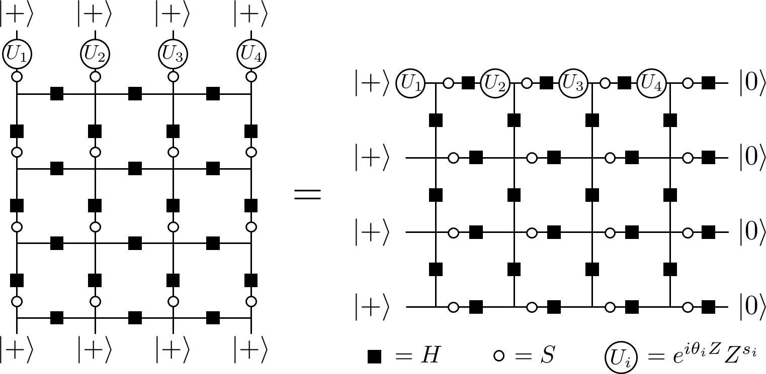
Figure 3: Tensor network representations of the left and right sides of Fig. 1.

Appendix B Propagation of byproduct operators

In the main text, we always assumed that a particular measurement outcome occurred for each measurement basis. In this section, we describe how to deal with the inherent randomness of measurement outcomes. In all cases described above, the effect of a “wrong” measurement outcome is to insert the operator $Z_{1}$ at that step of the computation. We show how to remove this by appropriately modifying the bases of all subsequent measurements, and discuss how this affects read-out at the end of computation.

A sequence of gates in our protocol is described by a sequence of angles $\theta_{i}$ defining the measurement bases. Suppose we obtain the desired outcome $|0^{\theta_{i}}\rangle$ for each measurement. The total evolution is then described by the equation,

$$\langle 0^{\theta_{1}},\dots,0^{\theta_{N}}|\psi_{k}\rangle=\langle R|U(\theta_{N})\dots U(\theta_{1})|L\rangle.$$ (10)

where $U(\theta)=T_{k}e^{i\theta Z_{1}}$. Now suppose we obtain the wrong outcome $|1^{\theta_{j}}\rangle$ at some site $j$, but obtain the desired outcome everywhere else. This inserts the operator $Z_{1}$ at the $j$-th step of computation,

$$\langle 0^{\theta_{1}},\dots,1^{\theta_{j}},\dots,0^{\theta_{N}}|\psi_{k}\rangle$$

$$=\langle R|U(\theta_{N})\dots U(\theta_{j})Z_{1}\dots U(\theta_{1})|L\rangle$$ (11)

$$=\langle R|T_{k}^{N-j+1}(Z_{1})\widetilde{U}(\theta_{N})\dots\widetilde{U}(\theta_{j+1})U(\theta_{j})\dots U(\theta_{1})|L\rangle$$

where we use the shorthand notation $T_{k}^{l}(\cdot)=T_{k}^{l}\cdot T_{k}^{l\dagger}$. In the second line, we have commuted the unwanted operator $Z_{1}$ to the end of the computation by writing $U(\theta_{i})\mapsto\widetilde{U}(\theta_{i})$ for all $j+1\leq i\leq N$ where,

$$\widetilde{U}(\theta_{i})=T_{k}^{i-j+1}(Z_{1})^{\dagger}U(\theta_{i})T_{k}^{i-j}(Z_{1}).$$ (12)

Now we observe that $U(\theta_{i})T_{k}^{i-j}(Z_{1})=T_{k}^{i-j+1}(Z_{1})U(\pm\theta_{i})$ where the sign is $-1$ only if $T^{i-j}(Z_{1})$ acts as $X$ or $Y$ on the first logical qubit, in which case it will anti-commute with $Z_{1}$, thereby flipping $e^{i\theta_{i}Z_{1}}\rightarrow e^{-i\theta_{i}Z_{1}}$. Then we have $\widetilde{U}(\theta_{i})=U(\pm\theta_{i})$. More precisely, let $\xi=(\xi^{X};\xi^{Z})$ be a $2k$-component binary vector such that Pauli operators are written as $V(\xi)=\bigotimes_{i=1}^{k}X_{i}^{\xi^{X}_{i}}Z_{i}^{\xi^{Z}_{i}}$, and define the matrices $t_{k}$ acting on these vectors by $V(t_{k}\xi):=T_{k}V(\xi)T_{k}^{\dagger}$. Then, we have,

$$\widetilde{U}(\theta_{i})=U((-1)^{(t^{i-j}\hat{Z_{1}})^{X}_{1}}\theta_{i}),$$ (13)

where $\hat{Z_{1}}=(0,\dots,0;1,0,\dots,0)$ is the vector representing the Pauli $Z_{1}$ and $(t_{k}^{i-j}\xi)^{X}_{1}$ denotes the first entry of the $X$-component of the vector $t_{k}^{i-j}\xi$.

Therefore, inserting the operator $Z_{1}$ at step $j$ has two effects. First, it flips the rotation angle of some future rotations in a pattern that is determined by $T_{k}$. This effect is counteracted by flipping the angle in the corresponding measurement basis, i.e. sharing a classical bit of information $(t_{k}^{i-j}\hat{Z_{1}})^{X}_{1}$ with all sites $i>j$ which says whether this measurement angle should be flipped or not. These bits are then updated every time a new measurement outcome is obtained. This modification of future measurement bases in terms of past measurement outcomes can also be interpreted as applying symmetry transformations to the chain after each measurement outcome Else et al. (2012b). These symmetries are described in Section D.

The second effect of inserting $Z_{1}$ is to modify the boundary vector $\langle R|\mapsto\langle R|T_{k}^{N-j+1}(Z_{1})$. This has a positive effect: since $\langle R|$ is initially in the state $\langle 0,\dots 0|$, this action will flip it (up to a sign) to another product state in the $Z$-basis that depends on $j$. In Appendix D, it is proven that the operators $T_{k}^{\ell}(Z_{1})$ generate all Pauli operators under multiplication. Therefore, for all product states in the $|0/1\rangle$ basis, there exists a sequence of measurement outcomes that will map $|R\rangle$ to that state. Because of this, repeating our computation many times allows us to estimate $\langle i_{1},\dots,i_{k}|\phi_{\mathrm{out}}\rangle$ for all $|i_{j}\rangle=|0/1\rangle$ where $|\phi_{\mathrm{out}}\rangle=U(\theta_{N})\dots U(\theta_{1})|L\rangle$.

Appendix C Proof of Theorem 1

Here we give the proof of Theorem 1 by explicitly constructing a universal gate set. The proof proceeds in a number of technical steps, but the main ideas come from Lemmas 1 and 2. Throughout this section, we let $\mathcal{P}_{k}$ denote the set of all Pauli operators on $k$ qubits, not including the identity operator. Given a set $S$ of Paulis, we let $\mathcal{A}_{S}$ denote the Lie algebra generated by $S$ under commutation. The first part of the Theorem applies to all values of $k$, but we first fix $k=4m-1$ with $m>0$ and explain how to extend to general $k$ at the end.

Lemma 1.

Consider a set of Pauli operators $\mathcal{S}$ whose elements have the form $P_{1}\otimes P_{2}$ where $P_{\alpha}\in\mathcal{P}_{k_{\alpha}}$ with $k_{\alpha}>2$. Suppose that (i) there is a set of operators $S_{1}=\{P_{i}\otimes I:i=1,\dots,M\}\subset\mathcal{S}$ which generate all operators $P\otimes I$ for $P\in\mathcal{P}_{k_{1}}$ under commutation and (ii) there is a set of operators $S_{2}=\{A_{i}\otimes B_{i}:i=1,\dots,M^{\prime}\}\subset\mathcal{S}$ such that $A_{i}\neq I$ and the operators $B_{i}$ generate all of $\mathcal{P}_{k_{2}}$ under multiplication. Then the Lie algebra $\mathcal{A}_{S}$ contains all of $\mathcal{P}_{k_{1}+k_{2}}$, i.e. $\mathcal{A}_{\mathcal{S}}=su(2^{k_{1}+k_{2}})$.

To use the above lemma, we will need to modify the operators $O_{k}(\ell)$ defined in the main text. Let us introduce the shorthand notation $O_{k}(-\ell)=O_{k}(p_{k}-\ell)$. Decompose these operators as $O_{k}(\ell)=\bigotimes_{i}O_{k}(\ell,i)$ where $O_{k}(\ell,i)$ is a Pauli operator acting on the $i$-th logical qubit and $i=1,\dots,k$ (the coordinates $\ell,i$ specify a column and row of the space-time evolution pictured in Fig. 2). Now define the following modified operators,

$$\widetilde{O}_{k}(\ell)=\begin{cases}\bigotimes_{i\notin 4\mathbb{N}}O_{k}(\ell,i)&\text{if }O_{k}(\ell,j)=I\text{ or }X\quad\forall j\in 4\mathbb{N}\\ 0&\text{else}\end{cases}$$ (14)

Therein, $4\mathbb{N}$ denotes all strictly positive multiples of 4. Let $\widetilde{\mathcal{O}}_{k}$ denote the set of all $\widetilde{O}_{k}(\ell)$. The purpose of defining this set of operators is as follows. Suppose that the state of the logical qubits is such that the qubits indexed by $i=4j$ for $j\in\mathbb{N}$ are in the state $|+\rangle$. Then $O_{k}(\ell)$ acts the same on this state as $\widetilde{O}_{k}(\ell)$ if the first case in Eq. 14 is fulfilled since $X|+\rangle=|+\rangle$. If the second case in Eq. 14 is fulfilled, then $\widetilde{O}_{k}(\ell)$ will change the state of at least one of the $4j$-th qubits. To prevent this from happening, we remove such operators from $\widetilde{\mathcal{O}}_{k}$ by setting them to 0. So, if we freeze every $4j$-th qubit in the state $|+\rangle$, we can treat $\widetilde{O}_{k}(\ell)$ as our effective generators of rotation. As an example, if $O_{k}(\ell)=Z_{3}X_{4}Z_{5}$, then $\widetilde{O}_{k}(\ell)=Z_{3}Z_{5}$.

Lemma 2.

For every $k=4m-1$, define a set of operators $\mathcal{S}_{k}\subset\widetilde{\mathcal{O}}_{k}$ as,

$$\mathcal{S}_{k}=\left\{\widetilde{O}_{k}(i):i\in\mathcal{I}_{k}\right\},$$ (15)

where,

$$\mathcal{I}_{k}=\left\{-1\right\}\cup\bigcup_{j=0}^{m-1}\{ 4j,4j+1,4j+2,$$ (16)

$$- 4j-2,-4j-3,-4j-4\}$$

Then $\mathcal{S}_{k}$ satisfies the conditions outlined in Lemma 1 with $k_{1}=3(m-1)$ and $k_{2}=3$, so $\mathcal{A}_{\mathcal{S}_{k}}=su(2^{3m})$.

In Fig. 2, the set $\mathcal{I}_{k}$ corresponds to the columns containing red boxes (along with $\ell=-1$).

Proof of Theorem 1. Combining Lemmas 1 and 2, we see that, if the logical qubits indexed by $4j$ for $j>0$ are initialized in the state $|+\rangle$, then we have a universal set of gates on the remaining $3(k+1)/4=3m$ logical qubits. Our initial state $|L\rangle$ satisfies this since all qubits start in the state $|+\rangle$. So we have shown that $su(2^{3m})\subset\mathcal{A}_{k}$ where $k=4m-1$. To extend this to all values of $k$, let $q$ be the largest number $4m-1$ that is less than or equal to $k$. Then, since $\widetilde{O}_{q}(\ell)\equiv\widetilde{O}_{k}(\ell)$ for $|\ell|\leq k$, where we use $\equiv$ to denote equivalence up to padding with identity operators, we can simply apply Lemma 2 with $k\rightarrow q$ to get $su(2^{3m})\subset\mathcal{A}_{k}$ where $m=\lfloor\frac{k+1}{4}\rfloor$.

To prove the second part of Theorem 1, we need to discuss efficiency. That is, we need to show that the universal gate set we have constructed can be implemented efficiently, meaning that the number of measurements needed to implement a desired gate scales efficiently in the number of qubits $k$. In conventional MBQC using a 2D cluster state as a resource, $N\sim kL$ measurements (and therefore $N$ physical qubits) are needed to simulate a circuit consisting of $L$ gates on $k$ logical qubits. Our protocol has two key differences. First, our set of elementary gates is not the usual set of single-qubit rotations plus a two-qubit gate, but rather the set of multi-qubit rotations generated by $O_{k}(\ell)$. However, the Solovoy-Kitaev theorem says that any universal gate set can efficiently simulate another Nielsen and Chuang (2002), so our unusual gate set does not give any significant overhead. A second difference is that we are restricted to performing the rotation generated by $O_{k}(\ell)$ only once per “clock cycle” of length $p_{k}$ for each $\ell$. In principle, if $p_{k}$ grew exponentially large in $k$ (which is the case for certain values of $k$), this restriction could mean that we cannot efficiently generate arbitrary gates. Luckily, we have the following Lemma,

Lemma 3.

For $k=2^{r}-1$, we have $p_{k}=3k+3$.

Therefore, $k$ can always be chosen such there is at most a linear overhead in the number of measurements and physical qubits as compared to usual MBQC. $\Box$

This linear overhead assumes that we perform only one rotation per clock cycle. In practice, it is likely that a given circuit can be compiled to our gate set in such a way that multiple rotations are performed per clock cycle, so this overhead will not saturate this linear bound.

Proof of Lemma 1. Let us introduce a function $\Lambda$ such that $\Lambda(P,Q)=1$ if the Pauli operators $P,Q$ commute and $\Lambda(P,Q)=-1$ if they anticommute. We note that $\Lambda$ is a bicharacter, meaning that $\Lambda(AB,C)=\Lambda(A,C)\Lambda(B,C)$ and similarly for the second input. Throughout this proof, we ignore all constant factors that may appear in front of Pauli operators, and write equality to mean equality up to a constant (for example, we may write $[X,Y]=Z$). Then, a commutator of two Pauli operators can be taken to be their product if they anticommute, and 0 if they commute. We prove the following statements to start:

First we show that, if $P_{1}\otimes Q_{1},P_{2}\otimes Q_{2}\in\mathcal{A}_{\mathcal{S}}$ with $P_{1},P_{2}\neq I$ and $Q_{1}\neq Q_{2}$, then there exists $P_{3}\neq I$ such that $P_{3}\otimes Q_{1}Q_{2}\in\mathcal{A}_{\mathcal{S}}$. Let $\Lambda(Q_{1},Q_{2})=s$ and identify a Pauli $P_{1}^{\prime}$ such that $P_{1}^{\prime}\neq P_{2}$ and $\Lambda(P_{1}^{\prime},P_{2})=-s$; such an operator $P_{1}^{\prime}$ always exists since $P_{2}$ always (anti)commutes with more than one other Pauli if $k_{1}>1$ ($P_{1}$ may already satisfy this, in which case the next step can be skipped). Now we want to show that $P_{1}^{\prime}\otimes Q_{1}\in\mathcal{A}_{\mathcal{S}}$. If $\Lambda(P_{1},P_{1}^{\prime})=-1$, then, since $P_{1}P_{1}^{\prime}\otimes I$ is in $S_{1}$ by assumption, we have $[[P_{1}\otimes Q_{1},P_{1}P_{1}^{\prime}\otimes I]=P_{1}^{\prime}\otimes Q_{1}\in\mathcal{A}_{\mathcal{S}}$. If $\Lambda(P_{1},P_{1}^{\prime})=1$, we can always find $P_{1}^{\prime\prime}$ such that $\Lambda(P_{1},P_{1}^{\prime\prime})=\Lambda(P_{1}^{\prime},P_{1}^{\prime\prime})=-1$. Then $P_{1}^{\prime\prime}\otimes I$ and $P_{1}P_{1}^{\prime}P_{1}^{\prime\prime}\otimes I$ are in $S_{1}$ by assumption, so $[[P_{1}\otimes Q_{1},[P_{1}P_{1}^{\prime}P_{1}^{\prime\prime}\otimes I],P_{1}^{\prime\prime}\otimes I]=P_{1}^{\prime}\otimes Q_{2}\in\mathcal{A}_{\mathcal{S}}$. Finally, since $\Lambda(P_{1}^{\prime}\otimes Q_{1},P_{2}\otimes Q_{2})=-1$ by construction, we have $[P_{1}^{\prime}\otimes Q_{1},P_{2}\otimes Q_{2}]=P_{1}^{\prime}P_{2}\otimes Q_{1}Q_{2}\in\mathcal{A}_{\mathcal{S}}$ and $P_{1}^{\prime}P_{2}\neq I$.

By assumption, the operators $B_{i}$ defined in the Lemma generate all of $\mathcal{P}_{k_{2}}$ via multiplication. Using the statement proven above, this means for all $Q\in\mathcal{P}_{k_{2}}$, there exists $P_{Q}\neq I$ such that $P_{Q}\otimes Q\in\mathcal{A}_{\mathcal{S}}$. By taking commutators of these elements with elements of $S_{1}$, any element of the form $P\otimes Q$ where $P,Q\neq I$ can be generated. Finally, we have $[P\otimes Q_{1},P\otimes Q_{2}]=I\otimes[Q_{1},Q_{2}]\in\mathcal{A}_{\mathcal{S}}$. Since every $Q\neq I$ can be written as $Q=Q_{1}Q_{2}$ for some $Q_{1},Q_{2}$ with $\Lambda(Q_{1},Q_{1})=-1$, we have $Q=[Q_{1},Q_{2}]$, so we generate all elements of the form $I\otimes Q$, which gives $\mathcal{A}_{\mathcal{S}}=\mathcal{P}_{k_{1}+k_{2}}=su(2^{k_{1}+k_{2}})$. $\Box$

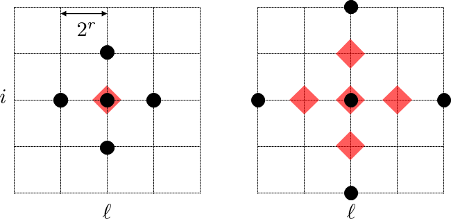
Figure 4: Illustration of the recurrence relation described by Eq. 18. On the left, we use black dots to represent the bits $a_{k}(\ell,i)$. The five marked bits, separated by a scale $2^{r}$, satisfy a relation which says they must sum to 0 mod 2, as stated in Eq. 17 for the case $r=0$. We use a diamond to indicate the center of this five-body relation. By summing five of these relations, with positions marked by the five diamonds, some of the bits involved in the relations cancel pairwise, and we retrieve the same recurrence relation over a distance $2^{r+1}$.

Proof of Lemma 2. Throughout this proof, we will make extensive use of the self-similar fractal nature of the space-time diagrams that describe the operators $O_{k}(\ell)$, as displayed in Fig. 2. To capture these patterns, we define the bits $a_{k}(\ell,i)$ and $b_{k}(\ell,i)$ such that $O_{k}(\ell,i)=Z_{i}^{a_{k}(\ell,i)}X_{i}^{b_{k}(\ell,i)}$, up to a phase. The following recurrence relation can be derived from Eq. 6,

$$a_{k}(\ell+1,i) \equiv a_{k}(\ell,i-1)+a_{k}(\ell,i)+a_{k}(\ell,i+1)$$ (17)

$$+a_{k}(\ell-1,i),\quad\text{for}\quad 1\leq i\leq k$$

where $\equiv$ denotes equivalence modulo 2. This relation is subject to periodic boundary conditions in the $\ell$-direction such that $a_{k}(-\ell,i)=a_{k}(p_{i}-\ell,i)$, and open boundaries in the $i$-direction such that $a_{k}(\ell,0)=a_{k}(\ell,k+1)=0$. The same relation holds for $b_{k}(\ell,i)$. Additionally, we have $b_{k}(\ell,i)=a_{k}(\ell+1,i)$. Concatenating these relations leads to a hierarchy of relations of the following form,

$$a_{k}(\ell+2^{r},i) \equiv a_{k}(\ell,i-2^{r})+a_{k}(\ell,i)+a_{k}(\ell,i+2^{r})$$ (18)

$$+a_{k}(\ell-2^{r},i),\quad\text{for}\quad 1\leq i\leq k$$

where $r\in\mathbb{N}$ is a number such that $2^{r}<k$. See Fig. 4 for a pictoral proof by induction of this equation. The boundary conditions satisfy $a_{k}(\ell,-i)=a_{k}(\ell,i-2)$ and $a_{k}(\ell,k+i)=a_{k}(\ell,k+2-i)$ for $1\leq i\leq k$. That is, the boundary conditions “reflect” indices outside of the range $1\leq i\leq k$ back into this range, as described for a similar scenario in Ref. Raussendorf, 2005 and discussed in more detail in the proof of Lemma 3. This recurrence relation captures the scale-invariance of the operator evolution.

As a first step, we need to understand the form of the operators $\widetilde{O}_{k}(\ell)$ which appear in the definition of $\mathcal{S}_{k}$. We can show that none of them are equal to 0, meaning that the corresponding operators $O_{k}(\ell)\in\mathcal{O}_{k}$ satisfy $O_{k}(\ell,j)=I\text{ or }X\quad\forall j\in 4\mathbb{N}$. This can be shown using Eq. 18 for $2^{r}=4$. Using this, and the initial conditions specified by our problem, we can show, for $m\in\mathbb{N}$,

$$O_{k}(\ell,4m)=\begin{cases}I\text{ or }X&\ell\in 4\mathbb{N}\\ I&\ell\in 4\mathbb{N}+1\\ I&\ell\in 4\mathbb{N}+2\\ I\text{ or }Z&\ell\in 4\mathbb{N}+3\\ \end{cases}.$$ (19)

Since $\mathcal{S}_{k}$ contains only operators with $\ell\notin 4\mathbb{N}+3$, this establishes the claim.

The rest of the proof proceeds by induction. We prove the Lemma for small $k$, and then we use the scale-invariance to extend this to arbitrarily large $k$. First, consider the base case of $k=7$, depicted in Fig. 2. The operators $\widetilde{O}_{7}(\ell)$ for $\ell=1,2,3,20,21,22,23$ generate all Paulis $P\otimes I$ where $P$ acts on the first three qubits (note that the operator $X_{4}$ contained in $O_{7}(20)$ is removed in the transition to $\widetilde{O}_{7}(20)$). This can be easily shown by numerically taking commutators until all 63 Paulis are generated. This gives the operators necessary to satisfy condition (i) of Lemma 1 with $k_{1}=3$ and $S_{1}=\{\widetilde{O}_{7}(\ell):\ell=1,2,3,20,21,22,23\}$. For the second condition of Lemma 1, write $\widetilde{O}_{7}(\ell)=A_{7}(\ell)\otimes B_{7}(\ell)$ where $A_{7}(\ell)=\bigotimes_{i=1}^{3}\widetilde{O}_{7}(\ell,i)$ and $B_{7}(\ell)=\bigotimes_{i=5}^{7}\widetilde{O}_{7}(\ell,i)$. We observe (again numerically) that the six operators $B_{7}(\ell)$ for $\ell=4,5,6,16,17,18$ generate all 63 Paulis acting on the last three qubits via multiplication (but not via commutation). This is a consequence of the repeating structures in the space-time evolution of the operators, shown by the red squares in Fig. 2. We also observe by eye that $A_{7}(\ell)\neq I$ for all $\ell$. Therefore, the set $S_{2}=\{\widetilde{O}_{7}(\ell):\ell=4,5,6,16,17,18\}$ satisfies condition (ii) of Lemma 1. This proves the Lemma for $k=7$.

Now, assume that we have proven the Lemma for some $k=4m-1$ with $m>2$, meaning we have shown that $\mathcal{S}_{k}$ satisfies the conditions of Lemma 1, such that $\mathcal{A}_{\mathcal{S}_{k}}=su(2^{3m})$. We want to show that $\mathcal{S}_{k+4}$ also satisfies the conditions of Lemma 1. Observe that $\widetilde{O}_{k+4}(\ell)\equiv\widetilde{O}_{k}(\ell)$ for all $\ell$ such that $|\ell|<k$, where we again use $\equiv$ to denote equivalence up to padding with identity operators. Then the set $S_{1}=\{\widetilde{O}_{k+4}(\ell):\ell=0,1,2,\dots,k-1,-1,-2,\dots,-k-1\}\equiv\mathcal{S}_{k}$ satisfies condition (i) of Lemma 1 with $k_{1}=3m$ by assumption.

To establish condition (ii) of Lemma 1, write $\widetilde{O}_{k+4}(\ell)=A_{k+4}(\ell)\otimes B_{k+4}(\ell)$ for $\ell=k+1,k+2,k+3,-k-3,-k-4,-k-5$ where $A_{k+4}(\ell)=\bigotimes_{i=1}^{k}\widetilde{O}_{k+4}(\ell,i)$ and $B_{k+4}(\ell)=\bigotimes_{i=k+2}^{k+4}\widetilde{O}_{k+4}(\ell,i)$. To understand the form of these operators, we use the recurrence relations. First, we have $O_{k}(\pm(\ell+4),i+4)=O_{k}(\pm\ell,i)$ for $\ell=0,\dots,k-4$ and $i=\ell,\dots,\ell+3$, as indicated by the solid red boxes in Fig. 2. This is because, for the specified values of $\ell$ and $i$, the relation for $2^{r}=4$ says that $a_{k}(\pm(\ell+4),i)=a_{k}(\pm\ell,i+4)$ (and similarly for $b_{j}(\ell,i)$) since all other terms in the relation are 0. Since we know from the proof for $k=7$ that the operators in the solid red boxes generate all operators acting on the corresponding three qubits under multiplication, we see that $B_{k+4}(\ell)$ satisfies this for qubits $i=k+2,k+3,k+4$. We now need to show that $A_{k+4}(\ell)\neq I$. This can be seen in Fig. 2 for $k=31$, and can again be shown using the recurrence relations in Eq. 18, this time for $2^{r}=8$. As above, the relations say that the operators in the dotted red boxes in Fig. 2 repeat for space-time steps of size 8. Since the operators contained in these dotted boxes are not the identity for small $k$, we have shown that $A_{k+4}(\ell)\neq I$. Therefore, the set $S_{2}=\{\widetilde{O}_{k+4}(\ell):\ell=k+1,k+2,k+3,-k-3,-k-4,-k-5\}$ satisfies condition (ii) of Lemma 1, and we have proven the Lemma. $\Box$

Proof of Lemma 3. This proof is very similar to that given in Ref. Stephen et al., 2019, but some modification is needed due to the open boundary conditions. To account for the open boundary conditions, we follow Ref. Raussendorf, 2005. Consider the circuit on an infinite chain $T_{\infty}=\lim_{k\rightarrow\infty}T_{k}$ with sites indexed by an integer $i\in\mathbb{Z}$. It is shown in Ref. Raussendorf, 2005 that the open boundaries effectively act as a mirror that reflects the information that is propagated out of the range $1\leq i\leq k$ back into that range. This reflection can be mimicked by adding “ghost images” of the operator evolution that start outside of this range, similar to the method of image charges from electrostatics. More precisely, the evolution on a finite chain is related to that on an infinite chain by the following equation,

$$T_{k}^{\dagger}Z_{i}T_{k}=T_{\infty}^{\dagger}\left[\prod_{n=-\infty}^{\infty}Z_{i+2n(k+1)}Z_{-i+2n(k+1)}\right]T_{\infty},$$ (20)

where operators on the right-hand side acting on qubits outside of the range $1\leq i\leq k$ are simply ignored. A similar condition holds for $T_{k}^{\dagger}X_{i}T_{k}$, and therefore for any product of Pauli operators.

We now transition to a more compact notation for describing the action of $T_{\infty}$, which is translationally invariant Schlingemann et al. (2008). As in Section B, let $\xi=(\xi^{X};\xi^{Z})$ be an infinite binary vector such that Pauli operators on the infinite chain are written, up to a phase, as $V(\xi)=\bigotimes_{i\in\mathbb{Z}}X_{i}^{\xi^{X}_{i}}Z_{i}^{\xi^{Z}_{i}}$. Now, we further condense this information by mapping the binary vector onto a polynomial vector as,

$$\begin{pmatrix}{\xi}^{X}\\ {\xi}^{Z}\end{pmatrix}\mapsto\begin{pmatrix}\sum_{i}(u^{i})^{\xi^{X}_{i}}\\ \sum_{i}(u^{i})^{\xi^{Z}_{i}}\end{pmatrix}.$$ (21)

where $u$ is a dummy variable. We denote both the binary and polynomial vectors as $\xi$. Then, we represent the $T_{\infty}$ as a $2\times 2$ matrix $t_{\infty}$ of polynomials by arranging

$$T_{\infty}(X_{0}) =Z_{0}=\begin{pmatrix}0\\ 1\end{pmatrix}:=t_{\infty}\begin{pmatrix}1\\ 0\end{pmatrix},$$ (22)

$$T_{\infty}(Z_{0}) =Z_{-1}Y_{0}Z_{1}=\begin{pmatrix}1\\ u+1+u^{-1}\end{pmatrix}:=t_{\infty}\begin{pmatrix}0\\ 1\end{pmatrix}$$

into columns of a matrix, giving,

$$t_{\infty}=\begin{pmatrix}0&1\\ 1&u+1+u^{-1}\end{pmatrix}.$$ (23)

Given a Pauli operator represented by a polynomial vector $\xi$, Eq. 20 tells us to look at the action of $t_{\infty}$ on the polynomial $\tilde{\xi}=q_{k}(u)(\xi+\bar{\xi})$ where $\bar{\xi}$ is obtained from $\xi$ by inverting every monomial $u^{i}\mapsto u^{-i}$ and $q_{k}(u)=\sum_{n=-\infty}^{\infty}u^{2n(k+1)}$. We want to show that, if $k=2^{r}-1$, then

$$t_{\infty}^{3k+3}\tilde{\xi}=(t_{\infty}^{3})^{2^{r}}\tilde{\xi}=\tilde{\xi}.$$ (24)

Translating back to operator notation, this result, combined with Eq. 20, would give $T_{k}^{3k+3}=I$.

Assume that $k=2^{r}-1$. To show that Eq. 24 is true, we use the Cayley-Hamilton theorem, which says that Gütschow et al. (2010),

$$(t_{\infty}^{3})^{2}=\mathrm{Tr}(t_{\infty}^{3})t_{\infty}^{3}+I.$$ (25)

Let us denote $\gamma=\mathrm{Tr}(t_{\infty}^{3})$. Another important result is that, for any polynomial $p(u)$, we have $p(u)^{2^{n}}\equiv p(u^{2^{n}})$ for any $n\in\mathbb{N}$. This holds because the coefficients of the polynomials are in $\mathbb{Z}_{2}$, so the cross terms cancel out each time $p(u)$ is squared. Combining this with Eq. 25, we have,

$$(t_{\infty}^{3})^{2^{r}} =((t_{\infty}^{3})^{2})^{2^{r-1}}=(\gamma t_{\infty}^{3}+I)^{2^{r-1}}$$ (26)

$$=\gamma^{2^{r-1}}(t_{\infty}^{3})^{2^{r-1}}+I.$$

It is straightforward to compute that,

$$\gamma=(u^{1}+1+u^{-1})(u^{2}+u^{-2}).$$ (27)

This gives,

$$\gamma^{2^{r-1}}q_{k}(u)=(u^{2^{r-1}}+1+u^{-2^{r-1}})(u^{2^{r}}+u^{-2^{r}})q_{k}(u).$$ (28)

As $q_{k}(u)=\sum_{n=-\infty}^{\infty}u^{n2^{r+1}}$, we have $(u^{2^{r}}+u^{-2^{r}})q_{k}(u)=0$ since the two terms are equal and the polynomials have $\mathbb{Z}_{2}$ coefficients. This means that when computing $(t_{\infty}^{3})^{2^{r}}\tilde{\xi}$, the first term in Eq. 26 is equal to zero, so we have $(t_{\infty}^{3})^{2^{r}}\tilde{\xi}=\tilde{\xi}$ as desired. This completes the proof. $\Box$

Appendix D SPT order in the resource states

In this section we derive the symmetries and SPT order of the states $|\psi_{k}\rangle$. To do this, we first define the states $|\widetilde{\psi}_{k}\rangle$ in the same way as $|\psi_{k}\rangle$ except with periodic boundary conditions, such that qubits 1 and $N$ interact with a $CZ$ each layer of the circuit. Let us assume for simplicity that the length $N$ is a multiple of the period $p_{k}$. The generalization of Eq. 4 for periodic boundary conditions, taking $\theta_{i}=0$ for all $i$, is,

$$\langle s_{1},\dots,s_{N}|\widetilde{\psi}_{k}\rangle=\mathrm{Tr}\left(A(s_{N})\dots A(s_{1})\right)$$ (29)

where $A(s)=U(0,s)=T_{k}Z_{1}^{s}$. This defines a translationally-invariant matrix product state (MPS) representation of the state $|\psi^{\prime}_{k}\rangle$ Cirac et al. (2021). As is generally the case for MPS, the symmetries of the state $|\widetilde{\psi}_{k}\rangle$ can be understood via the symmetries of the matrices $A(s)$. Using the binary vector notation for Pauli operators introduced in Section B, $A(s)$ satisfies the following relation,

$$V(t_{k}\xi)^{\dagger}A(s)V(\xi)=(-1)^{s\xi^{X}_{1}}A(s).$$ (30)

This relation can be concatenated $N$ times to derive a symmetry of the wavefunction,

$$\mathrm{Tr}\left(A(s_{N})\dots A(s_{1})\right)$$ (31)

$$=\left[\prod_{i=1}^{N}(-1)^{s_{i}(t_{k}^{i}\xi)^{X}_{1}}\right]\mathrm{Tr}\left(A(s_{N})\dots A(s_{1})\right)$$

which holds for any $\xi$, where $(t_{k}^{i}\xi)^{X}_{1}$ again denotes the first entry of the $X$-component of the vector $t_{k}^{i}\xi$. This translates to a symmetry $|\psi_{k}^{\prime}\rangle=u(\xi)|\psi_{k}^{\prime}\rangle$ where,

$$u(\xi)=\prod_{i=1}^{N}Z_{i}^{(t_{k}^{i}\xi)^{X}_{1}}$$ (32)

For example, the symmetry $u(\hat{Z_{1}})$, where $\hat{Z_{1}}=(0,\dots,0;1,0,\dots,0)$ is the vector representing the Pauli $Z_{1}$, is reflected in the top row of the space-time diagrams depicting the space-time evolution of the operators $O_{k}(\ell)$, see Fig. 2). At the end of this section, we prove that all $2^{2k}$ choices of $\xi$ lead to a different symmetry operator when $N$ is a multiple of $p_{k}$, so the representation $\xi\mapsto u(\xi)$ defines a $\mathbb{Z}_{2}^{2k}$ symmetry group of $|\widetilde{\psi}_{k}\rangle$. We also prove that this symmetry group can be fully generated by products of $u(\hat{Z_{1}})$ and its translations. Note that, if $N$ is not a multiple of $p_{k}$, the global symmetry group will be smaller, but the bulk symmetry, and therefore the SPT order, is not affected.

Having identified the symmetries of the resource states, we now ask whether they have non-trivial SPT order with respect to these symmetries. Our calculations used to derive the symmetry contain enough information to answer this question. Namely, Eq. 30 reveals that the representation of the symmetry acting on the virtual Hilbert space is $\xi\mapsto V(\xi)$. While the physical representation $\xi\mapsto u(\xi)$ is linear, meaning $u(\xi)u(\zeta)=u(\xi\oplus\zeta)$ where $\oplus$ denotes mod-2 addition, the virtual representation is projective with,

$$V(\xi)V(\zeta)=(-1)^{\xi^{T}\Lambda\zeta}V(\xi\oplus\zeta)$$ (33)

where $T$ denotes the transpose and $\Lambda=\begin{pmatrix}0&I_{k}\\ I_{k}&0\end{pmatrix}$ with $I_{k}$ the $k\times k$ identity matrix. The non-commutativity of the virtual representation of the symmetry implies the existence of non-trivial SPT order Pollmann et al. (2010); Chen et al. (2011); Schuch et al. (2011). In fact, this representation is a so-called maximally non-commutative representation, which is one where only the identity element commutes with all other elements Else et al. (2012a). Using the results of Else et al. (2012a), it is straightforward to show that this implies that the degeneracy of the zero-energy edge mode associated to the SPT phase is $\sqrt{|\mathbb{Z}_{2}^{2k}|}=2^{k}$, since this is the minimal dimension of irreducible representation satisfying Eq. 33. Maximally non-commutative phases are also exactly the phases to which the general results of Refs. Else et al., 2012a; Stephen et al., 2017, 2019 apply. Using these results, we can extend our MBQC protocol beyond the fixed-point states $|\psi_{k}\rangle$.

Finally, we prove two useful results about the symmetry representation $\xi\mapsto u(\xi)$ defined in Eq. 32. First we show that this is a faithful representation of $\mathbb{Z}_{2}^{2k}$. That is, if $u(\xi)=I$, then $\xi=0$. By definition, if $u(\xi)=I$, then $(t_{k}^{i}\xi)^{X}_{1}=0$ for all $i$. Since $T_{k}^{\dagger}X_{1}T_{k}=Z_{1}$, we have $(t_{k}^{i}\xi)^{X}_{1}=(t_{k}^{i+1}\xi)^{Z}_{1}$. So, if $(t_{k}^{i}\xi)^{X}_{1}=0$ for all $i$, then we also have $(t_{k}^{i}\xi)^{Z}_{1}=0$ for all $i$. So, in the operator evolution of $V(\xi)$ under $T_{k}$, the first row corresponding to $i=1$ remains empty (i.e. acted on by $I$) for all times. One can quickly convince oneself that, given the rules in Eq. 6, this is only possible if $\xi=0$. For example, if the first row is empty, then the second row must contain no $Z$ operators, since a $Z$ operator in the second row would spread to the first row in the next column, and therefore must also contain no $X$ operators. Progressing in this way, we conclude that every row must be empty, so $\xi=0$. Therefore, $u(\xi)=0$ implies $\xi=0$, so the representation is faithful.

Now, we prove that $u(\xi)$ can be expressed as a product of translations $u(\hat{Z_{1}})$ for all $\xi$. Translations of $u(\hat{Z_{1}})$ can be written as $u(t_{k}^{\ell}\hat{Z_{1}})$ for $\ell=0,\dots,p_{k}$. We want to prove that every vector $\xi$ can be expressed as a sum of the vectors $t_{k}^{\ell}\hat{Z_{1}}$. If this is true, then $u(\xi)$ is always a product of $u(t_{k}^{\ell}\hat{Z_{1}})$ for different $\ell$, since $u(\xi)u(\zeta)=u(\xi\oplus\zeta)$. The required condition is equivalent to the fact that the operators $O_{k}(\ell)\equiv T_{k}^{\ell\dagger}Z_{1}T_{k}^{\ell}$ generate the whole set of Pauli operators under multiplication. This is in turn equivalent to saying that the set $\{A(s_{1})\dots A(s_{L}):s_{1},\dots,s_{L}=0,1\}$ for $L=p_{k}$ spans the whole space of $2^{k}\times 2^{k}$ matrices, where $A(s)$ are the MPS tensors defined above. This property of an MPS is known as injectivity. Physically, an MPS has finite correlation length if and only if it admits an injective MPS representation Cirac et al. (2021). The states $|\psi^{\prime}_{k}\rangle$ certainly have finite correlation length, as they are generated from a product state with a quantum circuit, which implies that there exists an MPS representation of $|\psi^{\prime}_{k}\rangle$ given by some matrices $B(s)$ which satisfy injectivity. To prove that our matrices $A(s)$ are also injective, we first observe that $|\psi^{\prime}_{k}\rangle$ has a half-chain entanglement entropy of $S=k\log 2$, which is in fact a consequence of dual-unitarity Zhou and Harrow (2022). For an MPS defined by matrices of dimension $D$, the half-chain entanglement entropy is upper bounded by $\log D$. This means that $A(s)$, which has dimension $2^{k}$, has the minimal possible bond dimension. Therefore, by Proposition 20 of Ref. Molnar et al., 2018, there exists an invertible matrix such that $A(s_{1})\dots A(s_{n})=XB(s_{1})\dots B(s_{n})X^{-1}$ for large enough $n$, so the matrices $A(s)$ must also satisfy injectivity. This proves that $O_{k}(\ell)$ generate all Pauli operators under multiplication, which proves our desired result on $u(\xi)$.

Appendix E A non-universal dual-unitary Clifford circuit

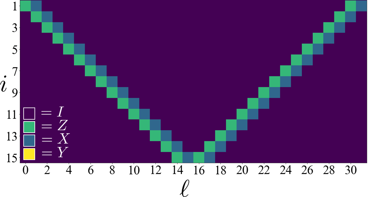
Figure 5: (a) The operator evolution inducted by ${T}^{\prime}_{k}$ which is obtained from $T_{k}$ by replacing $R\mapsto H$, with $k=15$. Each column represents an operator $O^{\prime}_{k}(\ell)$.

In this section we give an example of an alternate family of resource states which are also generated by a dual unitary circuit. They also share the feature that they are fixed-points of certain SPT phases. However, they differ in the fact that the set of implementable gates when using them as resource states for MBQC is not universal.

These states are defined as follows,

$$|\psi^{\prime}_{k}\rangle=T_{N}^{\prime k}\left(\bigotimes_{i=1}^{N}|+\rangle_{i}\right),$$ (34)

where,

$$T^{\prime}_{N}=\prod_{i=1}^{N}H_{i}\prod_{i=1}^{N-1}CZ_{i,i+1}.$$ (35)

These states differ from the states defined in the main text only by the substitution $HS\rightarrow H$. This corresponds to choosing $g=0$ in the kicked-Ising Hamiltonian. It is straightforward to show that most of the claims and constructions of the main text follow through with $T$ replaced by $T^{\prime}$. In particular, the circuit is still dual unitary such that viewing it sideways reveals a quantum computation in virtual space that is controlled by the measurement bases, where the set of unitary gates that can be performed are again rotations generated by operators of the form ${T^{\prime}_{k}}^{\dagger}Z_{1}T^{\prime}_{k}$.

The difference compared to the case presented in the main text is that these rotations no longer form a universal set. This is a consequence of the much simpler space-time evolution of the operators under conjugation by $T^{\prime}_{k}$, i.e. the operators $O^{\prime}_{k}(\ell)={T^{\prime}_{k}}^{\ell\dagger}Z_{1}{T^{\prime}_{k}}^{\ell}$, see Fig. 5. We see that $O^{\prime}_{k}(\ell)$ always has a basic form of a two-qubit operator (except at the boundaries) that is then translated along the virtual Hilbert space upon conjugation by $T^{\prime}_{k}$. This is a consequence of the fact that, if we regard $T^{\prime}_{k}$ as a Clifford quantum cellular automaton (CQCA), then it falls into the “glider” class as defined in Ref. Gütschow et al., 2010 (see also Ref. Stephen et al., 2019). This class of CQCA is defined by the existence of operators on which the CQCA acts as translation. On the other hand, if we regard $T_{k}$ as a CQCA, it falls into the “fractal” class Gütschow et al. (2010), which is less fine-tuned and has more complicated dynamics, as we can readily observe in our context.

As a consequence of the simple form of the operators $O^{\prime}_{k}(\ell)$, the algebra $\mathcal{A}^{\prime}_{k}$ that they generate under commutation is also simple. The size of this algebra turns out to grow quadratically in $k$, as we have $dim(\mathcal{A}_{k})=(k+1)(2k+1)$, which matches the dimension of $so(2(k+1))$. Such a polynomially growing algebra is not sufficient for universal MBQC (which requires the algebra to grow exponentially in $k$) Somma et al. (2006).

To see the non-universaility more explicitly, we show that the MBQC protocol using the state $|\psi^{\prime}_{k}\rangle$ can be efficiently simulated with a classical computer. Given the simple form of $O^{\prime}_{k}(\ell)$ displayed in Fig. 5, one can show that the elements of the algebra $\mathcal{A}^{\prime}_{k}$ each have a form that falls into one of three classes: $Y_{1}\dots Y_{i-1}U_{i}$, $U_{i}Y_{i+1}\dots Y_{k}$, or $U_{i}Y_{i+1}\dots Y_{j-1}V_{j}$ for $j\geq i$ where $U,V=X$ or $Z$. Let us modify the first two classes of operators by adding two new qubits at the ends of the chain, indexed by $i=0,k+1$, and defining corresponding operators, respectively, as $X_{0}Y_{1}\dots Y_{i-1}U_{i}$, $U_{i}Y_{i+1}\dots Y_{k}X_{k+1}$. Then, all three classes have the form $U_{i}Y_{i+1}\dots Y_{j-1}V_{j}$ where $0\leq i\leq j\leq k+1$. These operators correspond to quadratic fermionic operators after a Jordan-Wigner transformation. Therefore the expectation value,

$$\langle 0^{\theta_{1}},\dots,0^{\theta_{N}}|\psi^{\prime}_{k}\rangle=\langle R|e^{i\theta_{N}O^{\prime}_{k}(N)}\dots e^{i\theta_{1}O^{\prime}_{k}(1)}|L\rangle$$ (36)

where $|L\rangle$ is as defined before and $\langle R|$ can be any product state in the $Z$-basis, can be efficiently calculated using techniques from matchgate circuits (equivalently, fermionic linear optics) Valiant (2002); Terhal and DiVincenzo (2002); Jozsa and Miyake (2008). Therefore, the MBQC protocol can be efficiently classically simulated.

$k$	2	3	4	5	6	7
$p_{k}$	4	12	10	24	18	24
dim($\mathcal{A}_{k}$)	10	63	120	496	4095	8256
$\mathcal{A}_{k}$	$sp(2^{k})$	$su(2^{k})$	$so(2^{k})$	$so(2^{k})$	$su(2^{k})$	$sp(2^{k})$

(a) $\lambda_{i,t}=1$.

$k$	2	3	4	5	6	7
$p_{k}$	6	8	10	12	14	16
dim($\mathcal{A}_{k}$)	15	28	45	66	91	120
$\mathcal{A}_{k}$	$so(k^{\prime})$	$so(k^{\prime})$	$so(k^{\prime})$	$so(k^{\prime})$	$so(k^{\prime})$	$so(k^{\prime})$

(b) $\lambda_{i,t}=0$. $\left(k^{\prime}=2(k+1)\right)$

$k$	2	3	4	5	6	7
$p_{k}$	5	12	17	10	63	24
dim($\mathcal{A}_{k}$)	10	36	255	496	2016	8128
$\mathcal{A}_{k}$	$sp(2^{k})$	$sp(2^{k})$	$su(2^{k})$	$so(2^{k})$	$so(2^{k})$	$so(2^{k})$

(c) $\lambda_{i,t}=\delta({k-t\equiv 1}\mod 2$).

$k$	2	3	4	5	6	7
$p_{k}$	5	12	17	30	63	48
dim($\mathcal{A}_{k}$)	10	36	136	528	4095	8128
$\mathcal{A}_{k}$	$sp(2^{k})$	$sp(2^{k})$	$sp(2^{k})$	$sp(2^{k})$	$su(2^{k})$	$so(2^{k})$

(d) $\lambda_{i,t}=\delta({k-t\equiv 1}\mod 4$).

$k$	2	3	4	5	6	7
$p_{k}$	8	16	12	16	36	32
dim($\mathcal{A}_{k}$)	15	63	255	1023	4095	16383
$\mathcal{A}_{k}$	$su(2^{k})$	$su(2^{k})$	$su(2^{k})$	$su(2^{k})$	$su(2^{k})$	$su(2^{k})$

(e) $\lambda_{i,t}=\delta({i\equiv 1}\mod 2$).

$k$	2	3	4	5	6	7
$p_{k}$	16	8	40	32	56	16
dim($\mathcal{A}_{k}$)	15	28	255	1023	4095	16383
$\mathcal{A}_{k}$	$su(2^{k})$	$so(2^{k})$	$su(2^{k})$	$su(2^{k})$	$su(2^{k})$	$su(2^{k})$

(f) $\lambda_{i,t}=\delta({i\equiv 1}\mod 4$).

$k$	2	3	4	5	6	7
$p_{k}$	52	24	150	116	274	32
dim($\mathcal{A}_{k}$)	15	28	255	1023	4095	120
$\mathcal{A}_{k}$	$su(2^{k})$	$so(2^{k})$	$su(2^{k})$	$su(2^{k})$	$su(2^{k})$	$so(2(k+1))$

(g) $\lambda_{i,t}=\delta({i\equiv 1}\mod 16$).

$k$	2	3	4	5	6	7
$p_{k}$	12	8	20	12	28	16
dim($\mathcal{A}_{k}$)	15	21	255	528	4095	8128
$\mathcal{A}_{k}$	$su(2^{k})$	$sp(2k)$	$su(2^{k})$	$sp(2^{k})$	$su(2^{k})$	$so(2^{k})$

(h) $\lambda_{i,t}=\delta({i\equiv 1}\mod 2\text{ and }k-t\equiv 0\mod 2)$.

$k$	2	3	4	5	6	7
$p_{k}$	5	12	17	30	93	180
dim($\mathcal{A}_{k}$)	15	36	255	496	4095	8256
$\mathcal{A}_{k}$	$su(2^{k})$	$sp(2^{k})$	$su(2^{k})$	$so(2^{k})$	$su(2^{k})$	$sp(2^{k})$

(i) $\lambda_{i,t}=\delta(t=2)$.

$k$	2	3	4	5	6	7
$p_{k}$	5	7	9	11	13	15
dim($\mathcal{A}_{k}$)	10	21	36	55	78	105
$\mathcal{A}_{k}$	$sp(2k)$	$sp(2k)$	$sp(2k)$	$sp(2k)$	$sp(2k)$	$sp(2k)$

(j) $\lambda_{i,t}=\delta(t=1)$.

Figure 6: Numerical calculations of computational power at small $k$ for different choices of the matrix $\lambda_{i,t}$. The matrices are defined in terms of functions $\delta$ which return 1 if the contained expression is true and 0 otherwise. Tables 6(a) and 6(b) correspond to the cases considered in the main text and in Appendix E and are given for the sake of comparison. In table 6(b), we write $k^{\prime}=2(k+1)$ for compactness. Observe that all tables except 6(b) and 6(j) show that $\mathcal{A}_{k}$ appears to grow exponentially with $k$. In Table 6(g), the non-universality at $k=7$ is an artifact of a special relation between $k$ and the periodicity of $\lambda$; this case goes back to being universal at $k=8$.

Appendix F More examples of dual-unitary Clifford circuits

In this section, we investigate more examples of dual-unitary Clifford (DUC) circuits which increase the size of the unit cell for translation invariance in space or time. The goal of this study is to support the claim that the non-universality of the dual-unitary circuit studied in Appendix  E—as indicated by the polynomially-sized Lie algebra of generators of rotations—is fine-tuned, and that generic DUC circuits will have exponentially growing Lie algebras. To construct these examples, we consider the same basic gates $CZ$, $H$, and $HS$. At each time step, we apply $CZ$ to all nearest neighbours, followed by either $H$ or $HS$ on each qubit depending on both the spatial location of the qubit and the time step.

More precisely, we construct the following resource states,

$$|\psi_{k}(\lambda)\rangle=\left(\prod_{t=1}^{k}T_{N,t}(\lambda)\right)\left(\bigotimes_{i=1}^{N}|+\rangle_{i}\right)$$ (37)

where,

$$T_{N,t}(\lambda)=\prod_{i=1}^{N}H_{i}S_{i}^{\lambda_{i,t}}\prod_{i=1}^{N}CZ_{i,i+1}.$$ (38)

The matrix elements $\lambda_{i,t}=0,1$ determine whether or not $S$ acts on site $i$ at time-step $t$. For every choice of $\lambda$, the circuit defining $|\psi_{k}(\lambda)\rangle$ corresponds to a DUC circuit. In this notation, states $|\psi_{k}\rangle$ defined in the main text correspond to $\lambda_{i,t}=1$, while the states $|\psi^{\prime}_{k}\rangle$ defined in Appendix E correspond to $\lambda_{i,t}=0$.

We now numerically study a few examples of the above states. In order to be able to calculate a well-defined period of the virtual evolution, we enforce some periodicity on $\lambda_{i,t}$ in the time direction, but allowing a larger unit cell. For example, we could apply $S$ only on even number qubits, or only during even numbered time steps, and so on. The results are given in Table 6. We see that in all cases, except for the case studied in Appendix E and one other, the dimension of $\mathcal{A}_{k}$ appears to grow exponentially with $k$. For two of the universal cases, we also show the space-time evolution of the corresponding operators $O_{k}(\ell)$ in Fig. 7. We observe that these cases display complex structures that are in distinct contrast to the simple evolution of the non-universal case shown in Appendix E.

The second non-universal case 6(j) appears when $S$ is applied only on the first time step. This is equivalent to never applying $S$, and instead changing the initial state of the chain from $\bigotimes_{i=1}^{N}|+\rangle_{i}$ to $\bigotimes_{i=1}^{N}|y_{+}\rangle_{i}$ where $|y_{+}\rangle$ is the $+1$ eigenstate of $Y$. The computation that is induced in the spatial direction in this case is again matchgate circuit as in Appendix E. It is interesting to note that the family of states generated in this case corresponds to the family of spin chains studied in Ref. Verresen et al. (2017) which are Jordan-Wigner equivalent to free-fermion chains. We note that the non-universality of this case also appears to be fine tuned, as indeed applying $S$ only on the second time-step (instead of the first) as in Table 6(i) appears to give an exponentially growing algebra. This suggests that any small change in the dual-unitary circuit which drives it away from the matchgate case will lead to universality.

Finally, we note that the proof of universality (for the $\lambda_{i,t}=1$ case) given in Appendix C works by numerically proving universality for small $k$ and then taking advantage of scale invariance to prove universality for all $k$. Therefore, it is plausible that the universality at small $k$ shown for the examples in Table 6 can similarly be used to prove universality for all $k$.

Figure 7: Spacetime evolution of the $Z_{1}$ for the $k=63$ instance of the states defined by $\lambda_{i,t}$ as given in Table 6(g) (upper) and Table 6(d) (lower).