Abstract

Very-long-baseline interferometry (VLBI) is a challenging observational technique, which requires in-depth knowledge about radio telescope instrumentation, interferometry, and the handling of noisy data. The reduction of the raw data is mostly left to the scientists and demands the use of complex algorithms implemented in comprehensive software packages. The correct application of these algorithms necessitates a good understanding of the underlying techniques and physics that are at play. The verification of the processed data produced by the algorithms demands a thorough understanding of the underlying interferometric VLBI measurements. This review describes the latest techniques and algorithms that scientists should know about when analyzing VLBI data.

accepted for publication 10.3390/—— VLBI Science Applications Academic Editor: Received: date; Accepted: date; Published: date Software and techniques for VLBI data processing and analysis Michael Janssen¹*, Jack F. Radcliffe^2,3,4, Jan Wagner¹ Michael Janssen, Jack F. Radcliffe, Jan Wagner Correspondence: mjanssen@mpifr-bonn.mpg.de; Tel.: +49-228-525-431

1 Introduction

In recent years, several novel techniques and methods have been developed for the processing and analysis of very-long-baseline interferometry (VLBI) data, related primarily to the new needs and capabilities of novel VLBI instruments. For instance, the growing number of telescopes participating in large and global alliances of VLBI arrays (e.g., Gaylard et al., 2011; Deane, 2016; Matthews et al., 2018; Venturi et al., 2020; Barbosa et al., 2021), significant increases in bandwidths via improved gigabit per second (Gbps) recording rates (e.g., Whitney et al., 2013; Vertatschitsch et al., 2015), multi-frequency receiver capabilities (e.g., Han et al., 2008), advancements towards observing increasingly shorter wavelength emission to gain resolving power and counter self-absorption effects in the observed sources (e.g., Boccardi et al., 2017; Event Horizon Telescope Collaboration and et al., 2019), and prospects of the future next-generation Very Large Array (ngVLA, Selina et al., 2018; Murphy et al., 2018), VLBI capabilities of the Square Kilometre Array (SKA, Dewdney et al., 2009; Paragi et al., 2015), next-generation Event Horizon Telescope (ngEHT, Doeleman et al., 2019), as well as millimeter space VLBI observatories (e.g., Kardashev et al., 2014; Johnson et al., 2019; Fish et al., 2020; Gurvits et al., 2021).

Lately, the localization of a repeating fast radio burst (Marcote et al., 2017) and black hole images (Event Horizon Telescope Collaboration and et al., 2019; Event Horizon Telescope Collaboration and et al, 2022) have been continuum total intensity VLBI science highlights. More complex VLBI methods, which require a few additional steps, enable the study of magnetic field signatures through polarized synchrotron radiation, spectral line emission from astronomical masers, and wide fields of view combined with the VLBI resolving power.

With polarimetric VLBI (e.g., Gabuzda, 2018, 2020; Event Horizon Telescope Collaboration and et al, 2021a, b; Gabuzda, 2021), the role that magnetic fields play in the acceleration, collimation, and morphology of active galactic nuclei (AGN) jets can be studied across a wide range of scales. At the smallest scales, parameters of the central object responsible for producing the jet can be inferred to test for the presence of an event horizon, measure the spin of the compact object, and assess the role of the magnetic field in the jet launching.

Through spectral line VLBI (e.g., Habing, 1996; Momjian et al., 2003; Goddi et al., 2005; Hachisuka et al., 2006; Reid et al., 2009; Brunthaler et al., 2011; Goddi et al., 2011; Reid et al., 2013; Goddi et al., 2017; Moscadelli et al., 2019), maser emission from star forming regions, H I absorption, ejected circumstellar envelopes from giant stars, as well as gas in the vicinity of AGN that may be part of inflows or outflows can be mapped. Through Doppler shifts, the kinematics and physical conditions of the sources can be studied. Furthermore, angular-diameter distances to megamaser disk galaxies can be used for cosmology.

Wide-field VLBI (e.g., Garrett et al., 2001; Herrera Ruiz et al., 2017; Radcliffe et al., 2018; Spingola et al., 2018, 2019; Deller et al., 2019) enables powerful astrometric studies, the mapping of distances to pulsars in our galaxy, and the search for gravitationally lensed radio sources. Moreover, faint sources in the FOV can be detected, details in large extended structures such as AGN jet hotspots can be imaged when the instrument’s sensitivity is sufficient, and star formation radio emission can be distinguished from AGN activity in deep field studies.

Additionally, VLBI observations of spacecraft should be mentioned (e.g., Duev et al., 2012, and references therein). With a sufficiently stable and strong onboard radio emitter, spacecraft can be tracked with high accuracy, allowing for a wide range of planetary science applications, gravimetric studies, and tests of general relativity for example.

In this work, we review the typical sequence of VLBI processing steps and highlight the latest established open-source software packages and techniques. This information is targeted primarily at scientists who have obtained data from a VLBI observation and want to get an overview of the available tools for data processing and scientific analyses. We focus on the latest state-of-the-art algorithms and do not give a historical overview. We also do not discuss the scheduling of VLBI observations, which principal investigators (PIs) should do together with observatories and the help of the SCHED software. For a broad theoretical VLBI background, the reader is referred to Thompson et al. (2017). Definitions of technical terms used in this work that new VLBI users might be unfamiliar with are given in LABEL:tab:conventions.

VLBI measurements with the long baselines of the Low Frequency Array (LOFAR) are also possible, but require unique calibration strategies that are beyond the scope of this work. For example, due to the prevalence of direction-dependent effects, very low observing frequencies, and large data volumes. For details, the reader is referred to Morabito et al. (2022).

This review is structured as follows: Section 2 describes the correlation of VLBI data. Section 3 details the “signal stabilization”, which encompasses all data calibration steps needed before the data can be averaged in time and frequency. Section 4 outlines the amplitude gain corrections for telescopes that are needed for a flux density calibration in physical units. Section 5 explains how the sky brightness distribution of the observed source can be reconstructed from the calibrated data. Section 6 addresses how special science cases of polarization, spectral line, and wide-field VLBI are to be handled. Use-cases and algorithms for the synthetic generation of VLBI data are given in Section 7. A summary is presented in Section 8.

List of Abbreviations

AGN	Active galactic nuclei
ALMA	Atacama Large Millimeter/submillimeter Array
ASCII	American Standard Code for Information Interchange
ASIC	Application-specific integrated circuit
CLEAN	Imaging algorithm for an incomplete Fourier coverage
EHT	Event Horizon Telescope
EVN	European VLBI Network
EVPA	Electric vector polarization angle
EOP	Earth orientation parameter
FFT	Fast Fourier transform
FPGA	Field-programmable gate array
FOV	Field of view
FPT	Frequency-phase-transfer
Gbps	Gigabit per second
GMVA	Global mm-VLBI array
GPS	Global Positioning System
GPU	Graphics processing unit
GRMHD	General relativistic magnetohydrodynamics
HPC	High-performance computing
IDG	Image-domain gridder
IERS	International Earth Rotation and Reference Systems Service
JIVE	Joint Institute for Very Long Baseline Interferometry European Research Infrastructure
	Consortium
KVN	Korean VLBI Network
LCP	Left circularly polarized
LOFAR	Low Frequency Array
MAD	Magnetically arrested accretion disc
MERLIN	Multi-Element Radio Linked Interferometer Network
MFS	Multi-frequency synthesis
MPI	Message Passing Interface
MSC	Multi-scale CLEAN
MSSC	Multi-source self-calibration
MS-MFS	Multi-scale multi-frequency synthesis (combines MSC with MT-MFS)
MT-MFS	Multi-term multi-frequency synthesis
ngEHT	Next-generation Event Horizon Telescope
ngVLA	Next-generation Very Large Array
NRAO	National Radio Astronomy Observatory
RCP	Right circularly polarized
RML	Regularized maximum likelihood
PI	Principal investigator
PSF	Point spread function
RF	Radio frequency
RFI	Radio frequency interference
SANE	Standard and normal evolution accretion state
SEFD	System equivalent flux density
SFPR	Source frequency phase referencing
SKA	Square Kilometre Array
$S\,/\,N$	Signal-to-noise ratio
TCP	Transmission Control Protocol
TEC	Total electron content
UDP	User Datagram Protocol
UT	Universal Time
VERA	VLBI Exploration of Radio Astrometry
VGOS	VLBI Global Observing System
VLA	Very Large Array
VLBA	Very Long Baseline Array
VLBI	Very-long-baseline interferometry

Table 1: Basic terms, definitions, and concepts are listed here, which new VLBI users might be unfamiliar with or which might have slightly different meanings in other related works.

Name	Meaning
Telescope frontend	Equipment “directly attached to the front of a telescope”, used to detect and encode the sky signal. Receivers (e.g., bolometers) are frontend equipment.
Telescope backend	Equipment at the telescope that is used to process and store the signal from the frontend. Block Downconverters, which mix the sky signal down to a lower frequency range (heterodyning), analog-to-digital converters, which digitize the data, and data recorders, which store the digitized measurements on hard drives, are backend equipment.
Baseband data	The recorded data at a telescope that will be used for the correlation. More precisely, the filtered, down-converted, sampled, and quantized electric field measurements stored in the backends.
Signal stabilization	Described in Section 3: The collection of all post-correlation calibration measures, excluding the a priori flux density calibration (Section 4). The signal stabilization is often referred to as fringe-fitting, but it also involves additional steps, e.g., corrections for bandpass responses and corrections for atmospheric phase turbulence.
Delay	Residual post-correlation phase-slopes as a function of frequency (e.g., due to atmospheric path length differences). To be corrected in the signal stabilization step.
Rate	Residual post-correlation phase-slopes as a function of time (e.g., due to Doppler shifts) To be corrected in the signal stabilization step.
Fringe-fit FFT	The fast Fourier transform step of common fringe-fitting algorithms. Transforms the visibilities from time, frequency space into a rate, delay space, where the peaks are to be found. The height of the peaks corresponds to the strength of the signal.
Low $\nu$	An observing frequency below 20 GHz.
High $\nu$	An observing frequency above 20 GHz.
Allan deviation	A measure of frequency stability (Allan, 1966). An easy-to-follow derivation and description of the Allan deviation equation is given in Section 9.5.1 of Thompson et al. (2017).
VEX file	“VLBI EXperiment” file, which describes the VLBI setups and observing schedules in a standardized text format (https://vlbi.org/wp-content/uploads/2019/03/vex-definition-15b1.pdf).
FITS-IDI  file	“FITS Interferometry Data Interchange Convention” standardized file format for visibility and VLBI metadata built upon the upon the standard FITS format (https://fits.gsfc.nasa.gov/registry/fitsidi/AIPSMEM114.PDF).
ANTAB file	“Antenna table”, which contains station gain and system temperature information in a simple text file format (http://www.aips.nrao.edu/cgi-bin/ZXHLP2.PL?ANTAB).

2 Correlation

PIs are usually provided with correlated data, but it is instructive for scientists to understand the fundamentals of interferometric observations and upstream processing applied to their data.

There are two types of astronomical interferometers: Connected-element interferometers, and very long baseline interferometric networks that are used in astronomical and geodetic VLBI observations. Connected-element arrays can be “phased”, producing beamforming and phased-sum time domain signal output (e.g., Primiani et al. (2016); Matthews et al. (2018)). Such phased arrays can participate in VLBI, and are equivalent to a single large dish with a narrow beam.

For interferometry, the recorded baseband data (LABEL:tab:conventions) of all antennas are combined at a “correlator” computing system. In a connected-element interferometer, telescopes are connected over short (walkable) distances to a central correlator via RF-over-fiber or high speed network links, and share a common time and frequency standard. The short distances within an array permit very wide baseband signals (currently up to 64 GHz of bandwidth) from a large number of antennas (currently up to 10,000) to be transferred and processed at the array correlator in real time. The correlator usually employs hardware for the signal processing (FPGA, ASIC) due to power efficiency and operating cost considerations. With real-time correlation, the voluminous (often $>$ 10 Tbit/s aggregate) baseband data does not need to be stored. Only the final time averaged data products are kept.

VLBI networks consist of relatively few ($\lesssim$ 20) telescopes and, unlike in most connected-element arrays, they are often heterogeneous with different frequency tuning constraints, digital baseband bandwidths, baseband data formats, and no shared time and frequency standard. The large distances between telescopes located across the globe and in orbits around the Earth for space VLBI make real-time data transfer challenging.

Although there are recent VLBI hardware correlators, e.g., the 16-station x 8 Gbps Korean VLBI Network (KVN, Kim et al., 2004; Lee et al., 2011, 2014) and VLBI Exploration of Radio Astrometry (VERA, Kobayashi et al., 2003) correlator at the Korea-Japan Correlation Center (Lee et al., 2015), software correlators are currently more common. The flexible signal processing in software can better address possible complications that arise from the heterogenous set of telescopes. In addition, new observing modes are more rapidly implemented in software correlators.

2.1 Software Correlators

Two typical open source software VLBI correlators are DiFX Deller et al. (2007, 2011) and SFXC Keimpema et al. (2015). DiFX has a wide developer community and user base including the National Radio Astronomy Observatory (NRAO)/Very Long Baseline Array (VLBA, Napier et al., 1994), the Event Horizon Telescope (EHT, Event Horizon Telescope Collaboration and et al, 2019), and geodetic services. SFXC is more native to the European VLBI Network (EVN, see Porcas, 2010, and references therein) environment.

Being “embarrassingly parallel”, the correlation process is highly suited for cluster computing. Recently, graphics processing units (GPUs) are started to be used. One production GPU correlator is the 6-station x 16 Gbps near-realtime RasFX of the Quasar VLBI network Surkis et al. (2017); Shuygina et al. (2019). Other GPU-based VLBI correlators are under development or in a demonstrator stage, including an Extended-KVN GPU correlator and a possible correlator for VLBI space science Zhang et al. (2021). A GPU-accelerated version of DiFX is under development as well.

2.2 Station Clock Model

Typically, each VLBI telescope operates its own frequency standard, with an Allan deviation (Allan, 1966, LABEL:tab:conventions) of $<10^{-13}$ s/1 s and $<10^{-13}$ s/100 s to surpass atmospheric turbulence Rioja et al. (2012); Clivati et al. (2020). Receivers and backends are locked to the reference, and backends time-tag their digital baseband output data. An absolute time reference is provided by GPS, with an uncertainty of around $\pm 20$ ns due to ionospheric diurnal variation. Possibilities of sharing clock signals over long distances are currently being investigated (e.g., Krehlik et al., 2017; Clivati et al., 2020).

Without a shared clock signal, time-frequency transfer is emulated by a clock model that is applied at the correlator. The model consists of station clock offsets and drifts over time of the station frequency standards. Clock offsets are the differences measured between the backend data time-tag and the absolute Universal Time (UT). Drifts are measured via a continuous comparison against the GPS absolute time, usually fit to first order (linear drift) or sometimes to a higher order (acceleration) in space VLBI Likhachev et al. (2017).

Software correlators tend to be more flexible with their clock models than their hardware counterparts, handling offsets of several seconds at sub-microsecond granularity, and drifts of $10^{-9}$ s/1 s or larger.

2.3 Processing at the Correlator

The input for the correlator data processing are the baseband signals $E_{r}(t)$ from all telescopes. Appendix A describes how the recorded data are shipped to the correlation facility. Processing involves trivial computations at a high data rate. It produces time averaged mutual coherences between pairs of telescopes, analytically given by

$$\Gamma_{r_{1},r_{2}}{(u,v,\tau)}=\lim\limits_{T\to\infty}\frac{1}{2T}\int_{-T}^{T}E_{r_{1}}(t)E^{*}_{r_{2}}(t-\tau)\mathrm{d}t\;,$$ (1)

at $\tau\!=\!0$, over an integration time $T$, for telescopes at locations $r_{1}$ and $r_{2}$; see also Equation 15.1 in Thompson et al. (2017). Coherences between all telescope pairs and across their different spatial separations, or $(u,v)$-plane spatial frequencies, are called interferometric “visibilities” (cf. § 4.1 of Thompson et al. (2017)).

According to the van Cittert-Zernike theorem, these visibilities are the Fourier counterpart of the angular source brightness distribution, $I(l,m)$, related through

$$\Gamma_{r_{1},r_{2}}(u,v,0)=\iint I(l,m)\exp\left[-2\pi i(ul+vm)\right]\mathrm{d}l\mathrm{d}m\;;$$ (2)

see Equations 3.7 and 15.7 in Thompson et al. (2017). Here, the line-of-sight directions across the brightness distribution of the sky source are given by the unit vectors $(l,m,\sqrt{1-l^{2}-m^{2}})$. Visibility data produced by the correlator can thus be used for Fourier imaging – after a series of calibration steps described in later sections.

In practice the correlator determines $\Gamma_{r_{1},r_{2}}(u,v,n\Delta\tau)$ over a discrete range of time “delay lags”, $n\Delta\tau$, or equivalently in the spectral domain, spectral channels $N\Delta\nu$ across the baseband.

2.4 Correlator Delay Model

The correlator attempts to phase-align stations for maximum coherence to occur around $\tau=0$. This requires a delay model that includes the station clock models (Section 2.2), and several predicted geometric and propagation-path-related delays. These stem from observing geometry, Earth orientation, tidal/loading effects on station coordinates, tropospheric and ionospheric propagation, near-field wavefront and relativistic aberration effects, telescope orbit and orientation parameters for space VLBI, etc. The delay model can be produced with the common NASA GSFC Calc/Solve package or software specific to space VLBI or near objects (Gordon, 2004; Sekido and Fukushima, 2006; Likhachev et al., 2017).

Figure 1: VLBI observation and data processing. Per-telescope baseband and calibration data are collected during VLBI observations. Calibration data are bundled with the final visibility data release to the PI. Delay models for far-field VLBI are commonly derived via NASA GSFC CALC 9/10, for near-field VLBI via c5++ or others. Dashed boxes indicate optional processing, such as, pulsar processing, space VLBI antenna support, multi phase center for wide-field VLBI, spectral windowing (in SFXC) or custom channelization (zoom bands in DiFX). Correlation itself can run on hardware ranging from Raspberry PI, HPC clusters, to Cloud platforms.

The a priori delay model cannot predict all encountered delay components. Visibility data correlated with a wide enough delay range $n\Delta\tau$ and at sufficiently high temporal cadence allow unmodeled delay residuals, coming from random atmospheric turbulence for example, to be calibrated out via fringe-fitting (LABEL:tab:conventions) during post-processing (Section 3).

2.5 Correlator Parameters

Software correlators such as DiFX and SFXC are highly configurable and support various science and observing modes. Basic parameters are the PI-requested integration time and spectral resolution. Several additional data and settings flow into the correlator configuration, as illustrated in Figure 1.

In general, configuration files include a VEX file derived from the observing schedule, edited as necessary to describe the actual rather than nominal frequency setups and baseband data layouts each station used during the observation.

Depending on correlator features, additional parameters may include, e.g., 1) pulsar ephemeris data and binning/gating setups, 2) additional interferometric phase centers for wide-field VLBI within the telescopes’ primary beam, 3) settings for baseband spectral slicing or concatenation via DiFX “zoom” and “output” bands. These special band modes allow uniform-bandwidth visibility data records to be produced even for VLBI experiments where telescopes had incompatible frequency setups. 4) DiFX can also extract phase information of phase/pulse cal tone combs in the baseband data, if tones were injected during the observation. These combs are used for instrumental delay/phase calibration purposes, especially in geodetic VLBI. (5) At the VLBA, DiFX can extract on/off digital power levels of a synchronously switched calibration signal and produce continuous system temperature measurements (Section 4). (6) SFXC offers data windowing or weighted-overlap-add processing, which shape the frequency response of the spectral channels.

In networks, like the EVN and the VLBA, that observe frequently in standard modes and in a stable configuration, the preparatory steps and correlation can be largely automated and pipelined. In other instances and especially when there are technical changes at stations between sessions, or there is no automated collection of metadata (station clock models, actual tunings, updated coordinates, etc), the step of preparing initial correlator VEX and configuration files can involve extensive manual editing. For VLBI arrays that do not observe regularly with a consistent setup, multiple iterations of re-correlating plus data inspection on a small subset of scans are usually required, until one arrives at a final correlator configuration.

2.6 Correlator Output

After a correlation run (bottom of Figure 1) the output data are typically converted from a correlator-native format into the widely adopted FITS-IDI, Common Astronomy Software Applications (CASA) Measurement Set (MS), Haystack Observatory Postprocessing System (HOPS)/MkIV, or vgosDB NetCDF visibility data formats. Metadata or single-dish measurements (top of Figure 1) may further be attached to the visibility data-set as calibration tables. These may include system temperatures, antenna gain-elevation characteristics, weather data, flagging tables, and phase cal tones.

VLBI arrays typically observe in a circular polarization basis (through the use of quarter-waveplates), as the calibration of data from linear feeds is coupled to the different feed angle rotations at different antennas in a complicated way. If observations had some telescopes observing in linear rather than circular polarization, the visibilities will have a mixed polarization basis, which complicates the analysis of the data and is not supported by the FITS-IDI format. The VLBI Global Observing System (VGOS), some EVN, and also (sub)mm-VLBI observations that include the phased Atacama Large Millimeter/submillimeter Array (ALMA, Wootten and Thompson, 2009; Matthews et al., 2018) have to deal with this problem. Before release to the PI, the mixed polarization visibilities are converted into a purely circular basis with the PolConvert Martí-Vidal et al. (2016) program. The conversion requires telescope D-term and cross-polarization phase and gain characterization (Section 6.1). The ALMA Phasing Project quality-assurance (QA2) deliverables provide these parameters a priori for ALMA Goddi et al. (2019). Alternatively, parameters can be derived from the visibilities themselves, via a PolConvert calibration pass on unpolarized sources.

3 Signal stabilization

As described above, the correlator delay models are not perfect, which leads to residual delays and rates being present in the visibility data. Additionally, corrections for atmospheric phase fluctuations and instrumental bandpasses, where telescopes exhibit phase and amplitude variations over their frequency response, are usually not applied at the correlator. Post-correlation processing steps are therefore used to stabilize the source signal, ideally to remove all errors in the data down to the thermal noise. This allows us to average the data significantly in time and frequency, with limits set only by the structure and variability of the observed source in the presence of thermal noise only. In practice, the signal-to-noise ratio ($S\,/\,N$) of the data limits the degree to which data errors can be solved for. Without the signal stabilization steps, baseline-based errors will be frozen into the data due to phase decoherence, delay errors, and imperfect bandpass responses for example.

Instrumental errors such as amplitude and phase bandpasses, phase and delay offsets between analog frequency bands, and polarization imperfections of the receivers (Section 6.1), are stable or drift only slowly over the course of observations. VLBI scans on bright calibrators can thus be used to solve for these effects. Some telescopes inject and log phase/pulse cal signals into their signal chain (Section 2.5). These signals appear as weak periodic spectral lines (and should therefore not be used for spectral line observations) and can be used to estimate instrumental delay errors.

A common fringe-fitting method is to pick a reference station, transform the visibilities on baselines to that station into the delay-rate space with a fast Fourier transform (FFT), and to pick delay and rate estimates at the peak location in the two-dimensional FFT space Alef and Porcas (1986). The delay, rate, and phase is set to zero for the reference station and the FFT peaks are used as starting guesses for the station-based delays and rates of all other antennas. Additionally, the FFT $S\,/\,N$s (LABEL:tab:conventions) can serve as a threshold to distinguish between detections and non-detections. Finally, the data from all baselines on which the source is detected are used to refine the starting guesses and obtain final delay, rate, and phase solutions with a least-squares solver based on an assumed source model Schwab and Cotton (1983). The default assumption of a point source models usually does not lead to noticeable errors compared to the thermal noise (Event Horizon Telescope Collaboration and et al, 2019). Exceptions are highly sensitive arrays with a low thermal noise or geodesy experiments, where source structures might prevent reaching the required accuracy on the delays. If necessary, an iterative approach can be employed, where an image is first reconstructed (Section 5) using data calibrated with the assumption of a point source, that image is then used as source model to fringe-fit the data again, and the data with this improved calibration is then used to create a final image. Alternatively, it is possible, although computationally very expensive, to solve for the combined fringes and source structure using a Bayesian approach (Natarajan et al., 2020).

Unlike instrumental errors, the residual post-correlation delays, rates, and atmospheric phase fluctuations are source/direction-dependent. In cm-VLBI experiments, atmospheric errors are moderate and calibration solutions can be transferred from nearby calibrators to the science target. The closer the calibrator is to the science target, the better are the results; ideally both are within the same telescope primary beams. If the in-beam calibrator is weak, a “bi-gradient phase referencing” (Doi et al., 2006) can be employed, where a further away very bright source is used to detect a closer weak calibrator via phase-referencing, from which phase-referencing is then used to detect the very weak science target. Two col-linear aligned calibrators on opposite sides of a target source can be used for an improved correction of atmospheric errors (Fomalont and Kopeikin, 2002). With three or more calibrators, a two-dimensional phase screen of the atmosphere can be corrected for via two-dimensional interpolation of antenna phases using a “MultiView” technique (Rioja et al., 2017; Hyland et al., 2022). At high observing frequencies, dominant path delay uncertainties are caused by the troposphere. Akin to geodesy VLBI, “geodetic blocks” of $\sim$ 10 sources can be observed in short succession to accurately determine the zenith tropospheric delays at each telescope (Reid and Honma, 2014). Phase-referencing allows for astrometric measurements of the science target with respect to calibrator sources. At mm wavelengths, the science target itself has to be fringe-fitted and must therefore be bright enough to be detected within atmospheric coherence times or incoherent averaging has to be used (Rogers et al., 1995).

With multi-frequency receivers, it is possible to transfer phase solutions across bands to extend the coherence time at the higher frequencies and enable the detection of weaker sources. A simple frequency-phase-transfer (FPT) removes short-timescale tropospheric phase errors but does not allow for astrometric source registration. This technique can be combined with a phase-referencing between multiple targets as “source frequency phase referencing” ((SFPR), Rioja et al., 2008; Rioja and Dodson, 2011; Rioja et al., 2014, 2015). SFPR works at mm wavelengths, removes slowly varying residual ionospheric and instrumental effects not captured by the FPT, enables astrometry, and allows for longer on-source VLBI scans as well as longer telescope slewing times to calibrator sources that are further away, since the fast tropospheric phase errors have been removed by the FPT. Rioja and Dodson (2020) provide an outlook of high-precision astrometry measurements that will be enabled with future instruments and surveys.

The complex post-correlation data in its multi-dimensional polarization (correlation products), frequency, time, and baseline space has a considerable size and is challenging to handle. Particular difficulties can arise in heterogeneous VLBI arrays, where different stations may require different treatments, results may be dominated by the measurements (and potential systematics) of the most sensitive telescope(s), and varying station sensitivities may make a uniform data reduction difficult. For example, calibration solutions with a high time-and/or frequency resolution can be obtained for the sensitive telescopes, while large solution windows might be required to accumulate enough $S\,/\,N$ for the less sensitive telescopes, even when all baselines are used. For these considerations, array geometry also plays an important role; high $S\,/\,N$ data from the large scale emission of resolved sources can be obtained for smaller dishes if they have short baselines to more sensitive telescopes.

Errors in the data, which can typically be traced back to single antennas, are often not trivial to find; a variety of diagnostic tools and visualizations that make different cuts through the data are needed. Some – but typically not all – errors can be identified at the signal stabilization step. Appendix B provides an overview of how bad data can be identified and dealt with at the different data reduction stages. Calibration errors are easily baked into the data and can have substantial effects on the final scientific results. A typical order of VLBI calibration operations are shown in LABEL:fig:calibrationrFlow. Comprehensive and well-tested software suites are generally used for the primary calibration steps. The most common software packages are described below. Note that tools for the flux density calibration (Section 4), imaging (Section 5), as well as advanced calibration methods for polarimetry (Section 6.1), spectral lines (Section 6.2), and wide fields of view (Section 6.3) are implemented in several of these packages.

3.1 AIPS

The Astronomical Image Processing System (AIPS) (Greisen, 2003) is currently the most-widely used tool for the post-correlation calibration of VLBI data. The common visibility input data format that is produced by modern VLBI correlators is FITS-IDI. The calibrated output data are saved as UVFITS file to disk.

With AIPS, ionospheric corrections based on a priori maps of the global TEC can be applied to the data for an improved astrometry. Furthermore, the applied fringe corrections from the correlator can be improved with a posteriori determined IERS Earth Orientation Parameters. Finally, pulse cal signals can be used to calibrate instrumental effects.

Several hundred tasks are available within AIPS, covering all standard data calibration and analysis steps as well as advanced methods, such as computing the statistics on Allan Variances (ALVPR task), modeling of a gravitational lenses (GLENS), and optimizing configurations of telescope arrays (CONFI), to name a few examples.

The AIPS cookbook can serve as a detailed guide to typical VLBI data reduction pathways, where the needed AIPS tasks and their parameters are described for each step. Additionally, several generically useful VLBI tips and tricks are given.

3.1.1 ParselTongue

ParselTongue (Kettenis et al., 2006) is a Python interface for AIPS. It allows the user to run AIPS tasks, access calibration and visibility data, and to script their data processing. A ParselTongue pipeline is currently used for EVN pipelining operations.

3.2 CASA

The CASA software (McMullin et al., 2007, Emonts et al. in prep.) and its underlying suite of C++ “casacore” libraries are widely used for the processing of connected-element-interferometer radio data (e.g., from ALMA and the VLA) and also single-dish radio observations. (e.g., Thompson et al., 1980; Wootten and Thompson, 2009; Dewdney et al., 2009; van Haarlem et al., 2013). Initiated by the “BlackHoleCam” project (Goddi et al., 2017), CASA has been recently upgraded with VLBI capabilities, which are now supported and further developed by the Joint Institute for VLBI ERIC (JIVE) and NRAO (Van Bemmel et al., 2022). The input visibility can be in the native, locally stored MS format or FITS-IDI files, which will be loaded and converted to a MS. The final calibrated visibilities are stored together with the raw data in the MS and can also be exported as UVFITS files.

The CASA calibration framework is based on the Hamaker-Bregman-Sault measurement equation, a powerful mathematical framework for interferometric calibration problems, including direction-dependent effects (Hamaker et al., 1996; Smirnov, 2011a, b, c, d). Unlike AIPS, CASA stores the visibility data (in MS format) and calibration tables (in a MS-like format) separately on disk in the working directories.

The fringe-fitter and all standard CASA tasks can make use of a source model to improve calibration accuracy. The source model information is stored in the MS when the imaging is done within CASA (Section 5) or when an external FITS image is loaded. Ionospheric TEC corrections can also be done in CASA. Additionally, the fringe-fitter has the capability of solving for dispersive delays from the ionosphere.

Development plans for the short-term future include the handling of pulse cal data, an improved handling of irregularly spaced frequency channels when performing multi-band fringe-fitting, EOPs correction and a general accountability of the correlator model (Van Bemmel et al., 2022).

The next-generation CASA (ngCASA) project will improve the hardware scalability significantly, particularly the speed with which large data volumes from future instruments can be accessed and processed, by using off-the-shelf Python libraries like Dask (Rocklin, 2015) and xarray (Hoyer and Hamman, 2017).

3.2.1 rPICARD

CASA has a convenient toolkit for extensive visbility and calibration data access, which allows users to easily automate their data processing. This led to the development of a generic VLBI calibration pipeline, the Radboud PIpeline for the Calibration of high Angular Resolution Data (rPICARD), which is based on CASA (Janssen et al., 2018, 2019; Event Horizon Telescope Collaboration and et al, 2019). rPICARD employs flexible calibration strategies that work for any array and also synthetic VLBI data (Blecher et al., 2017; Natarajan et al., 2022).

rPICARD uses MPI for scalability and a custom robust scalar bandpass calibration method. The ionospheric dispersive delay and Faraday rotation correction is done with standard CASA tasks using TEC files from NASA’s Crustal Dynamics Data Information System. Fringe-fitting is done with the CASA Schwab-Cotton algorithm Schwab and Cotton (1983) and a simple single-source phase referencing method is implemented in rPICARD. Instrumental phase, delay, and bandpass effects are corrected by utilizing all scans on calibrator sources. For corrections of atmospheric phase turbulence at high observing frequencies, the fringe-fitting is done on a segmentation time, which is optimized based on the expected atmospheric coherence time at the observing frequency and the $S\,/\,N$ of the fringe detections. Figure 3 shows this two-step fringe-fitting approach, where fringe detections are first obtained over VLBI scan durations and residual atmospherically-induced errors are subsequently calibrated out on short segmentation times.

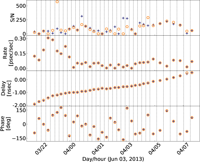
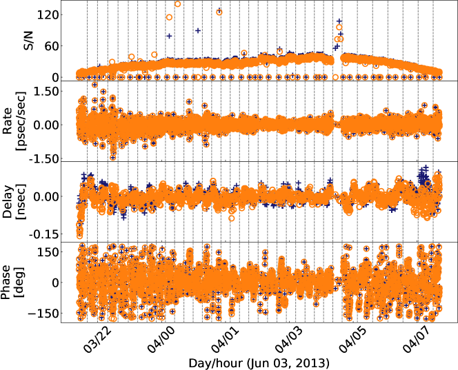
Figure 3: Example fringe solution diagnostics from rPICARD of M87 observed at 43 GHz with the VLBA (project code BW0106). Dashed lines show scan boundaries. Crosses and circles correspond to RCP and LCP, respectively. Top: Gross per-scan solutions. Bottom: Residual atmospheric corrections on adaptive segmentation timescales after the solutions from the top panel have been applied to the data.

Next to the aforementioned methods, which are implemented through standard CASA methods, rPICARD also has a few custom capabilities: 1) Exhaustive baseline searches to an arbitrary order are performed for non-detections to a primary reference antenna (Appendix D in Janssen et al., 2019). 2) The same rate solutions are applied to all polarization channels and a simple nearest-neighbor algorithm is used to re-reference all fringe solutions to a single antenna for the stability of polarized source signals. 3) Robust solutions for atmospheric opacities are derived with estimations of the atmospheric temperature from the ATM software (Pardo et al., 2001).

rPICARD can be obtained from a Bitbucket repository and for every version of the pipeline, Docker and Singularity containers are available (details are given in the README file of the pipeline repository).

3.2.2 VPIPE

The VLBI PIPEline (VPIPE) pipeline is an end-to-end CASA-based VLBI pipeline designed for mid-frequency ($\sim\mathrm{GHz}$) observations. It currently supports the EVN, VLBA and LBA networks. The pipeline employs similar steps to the rPICARD pipeline (§ 3.2.1) including TEC corrections, phase referencing via fringe fitting, and self-calibration.

Originally designed for the high data volumes associated with wide-field VLBI data (typically 10–50 TB), the pipeline utilises MPI-CASA and HPC parallelism provided by cluster scheduling software, such as SLURM and PBS Pro, for enhanced scalability. This allows the pipeline to process data quickly and efficiently, and permit the processing of “multiple phase centre observing” correlated data within short timescales (see § 6.3) (Deller et al., 2011). VPIPE is designed to be highly modular and supports containerization technologies, such as Singularity. This enables the user to easily add extra processing/analysis steps that uses custom scripts or software packages.

The pipeline incorporates advanced direction-dependent calibration steps needed for wide-field VLBI data. These include multi-source self-calibration (MSSC; see § 6.3), and primary beam correction schemes. This can be conducted in the $(u,v)$ or image plane. Correcting for these allows the pipeline to reduce noise levels, improve the dynamic range, increase the effective field-of-view, and ensure consistent flux density scales across the primary beam.

3.2.3 The e-MERLIN CASA Pipeline

The e-MERLIN CASA Pipeline (eMCP) is a Python pipeline that is designed for use with e-MERLIN data. It currently supports continuum and spectral line observations. The pipeline uses CASA-based VLBI tools, such as baseline and global fringe-fitting routines, to perform phase-referencing and self-calibration with parameters that are tailored for the e-MERLIN array and the observing frequency. The pipeline adopts other software tools such as AOFlagger (Offringa et al., 2012) and WSClean (Offringa et al., 2014) to address the challenging RFI environment and large image sizes often required.

Since 2019, eMCP has been incorporated as the official pipeline for the processing and delivery of e-MERLIN data to the users. As a result, it contains a suite of advanced quality assessment tools, displayed through a web-interface, that permit the user easily assess the quality of the calibration and images of the science targets.

3.2.4 JIVE EVN continuum Jupyter notebooks

EVN users are provided with a ParselTongue-based pipeline-calibrated version of their data by JIVE. Additionally, a CASA-based pipeline for EVN continuum is under development at JIVE, which will run in a Jupyter notebook (Keimpema et al., 2020; Van Bemmel et al., 2022) With this notebook, users will be able to start with a default set of parameters and steps used to calibrate EVN data, which can then be adjusted and refined to produce science-ready data.

3.3 EHT-HOPS

HOPS is a collection of basic VLBI functions like fringe-fitting, which are sufficient for the current needs of geodetic analyses (Whitney et al., 2004). However, HOPS is not as flexible as AIPS and CASA and lacks a few capabilities, which prevents a full scientific data analysis. The missing features will be implemented in an updated next-generation HOPS (ngHOPS) software package.

In the meantime, an “EHT-HOPS” (Blackburn et al., 2019; Event Horizon Telescope Collaboration and et al, 2019) pipeline has been designed, which augments HOPS with custom Python scripts to enable the full reduction of data from the EHT and Global mm-VLBI Array (GMVA) when ALMA is participating in the observations (Issaoun et al., 2019; Event Horizon Telescope Collaboration and et al, 2019). A least-squares solver is used to find station-based delay and rate solutions from the baseline-based estimates that HOPS can solve for Alef and Porcas (1986). High $S\,/\,N$ detections on bright calibrators are used to solve for bandpass effects. A piece-wise polynomial phase model is fitted directly to the visibilities to correct for atmospheric phase turbulence. To avoid over-fitting, phase corrections for each spectral window are obtained from a fit to all other spectral windows in the data. Relative complex gains between polarization channels are fitted to facilitate polarimetric analyses.

EHT-HOPS and rPICARD are used to produce science-ready data from the EHT (Event Horizon Telescope Collaboration and et al, 2019; Kim et al., 2020; Janssen et al., 2021; Event Horizon Telescope Collaboration and et al, 2022).

3.4 PIMA

PIMA (Petrov et al., 2011) is a specialized data reduction program, which can be used to accurately distinguish fringe detections from non-detections. PIMA is primarily employed for space VLBI experiments, because its fringe-fitter can solve for an acceleration (second-order rate) term. As space VLBI is beyond the scope of this work, we will not consider PIMA further.

4 Flux density calibration

After the signal stabilization, the correlation coefficients in units of thermal noise are normalized to unity autocorrelations and scaled corresponding to idealized analog correlation amplitudes. Ignoring baseline-dependent amplitude losses (such as de-correlation from data averaging), visibilities $\mathcal{V}_{ij}$ can be obtained in flux density units of Jansky (Jy) by calibrating the complex correlation coefficients $r_{ij}$ of the baseline connecting stations $i$ and $j$ with the a priori estimated system equivalent flux density (SEFD) sensitivities of our antennas,

$$\mathcal{V}_{ij}=\frac{1}{\eta_{Q}}\sqrt{\mathrm{SEFD}_{i}\mathrm{SEFD}_{j}e^{\tau_{i}+\tau_{j}}}r_{ij}\;.$$ (3)

Here, $\eta_{Q}$ is a correction factor for the digital quantization efficiency (Thompson et al., 2017); for 2-bit sampling, we have $\eta_{Q}\approx 0.88$. To correct for atmospheric attenuation of ground-based millimeter and submillimeter observations and thereby measure $\mathcal{V}_{ij}$ “above the atmosphere”, $e^{\tau}$ correction factors are applied. Here, $\tau_{i}$ is the mean atmospheric opacity along the line of sight signal path of antenna $i$.

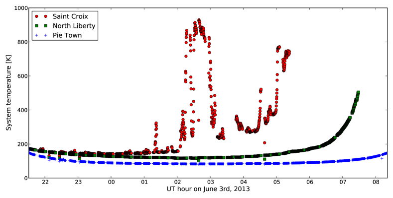
Figure 4: Example of effective (opacity-corrected) system temperatures measured by three VLBA antennas from observations of M87 at 43 GHz (project code BW0106). Pie Town system temperatures show slight increases at the beginning and end of the observing track, where the source is at a low elevation. The source sets at the end of the track for the North Liberty station, which causes an increases in system temperature. Bad weather is responsible for the highly variable system temperature measurements at Saint Croix.

The SEFDs are based on measured system temperatures $T_{\mathrm{sys}}$, the telescope gain $\mathcal{G}$ as a function of elevation, and the phasing efficiency $\eta_{\mathrm{ph}}$ for phased arrays: $\mathrm{SEFD}\propto\eta_{\mathrm{ph}}^{-1}\mathcal{G}^{-1}T_{\mathrm{sys}}$. Hot-load calibration scans measure the effective system temperature $T_{\mathrm{sys}}e^{\tau}$ directly and thereby immediately satisfy Equation 3 (Ulich and Haas, 1976). For noise-diode-based $T_{\mathrm{sys}}$ measurements, $\tau$ must be estimated after the fact. A common approach is to first approximate the system temperature as $T_{\mathrm{sys}}\simeq T_{\mathrm{rx}}+\left(1-e^{-\tau}\right)T_{\mathrm{atm}}$, where $T_{\mathrm{rx}}$ and $T_{\mathrm{atm}}$ are the two dominant noise terms, corresponding to receiver and atmospheric temperatures, respectively. Then, $T_{\mathrm{rx}}$ is estimated by extrapolating $T_{\mathrm{sys}}$ to zero airmass and an atmospheric model is used to estimate $T_{\mathrm{atm}}$ from weather parameters measured at the telescope. The $T_{\mathrm{sys}}$ measurements themselves can subsequently be used to estimate $\tau$ (Section 4.3 in Janssen et al., 2019). Examples of opacity-corrected system temperatures are shown in Figure 4.

The calibration metadata, gathered as a priori gain and system temperature information from all telescopes, are commonly stored in simple ASCII text files following the ANTAB format. Note that invalid entries are often marked with a value of $999$ or $-999$. Auxiliary weather information that might be needed to estimate $T_{\mathrm{atm}}$ for an opacity correction is usually attached to the visibility data format. Otherwise, it can be loaded from an ASCII text file (by AIPS and rPICARD as described in Janssen et al. (2019)).

4.1 Software implementations

AIPS, CASA/rPICARD, and EHT-HOPS post-processing scripts can be used to extract SEFDs from ANTAB tables and subsequently perform the a priori flux density calibration. AIPS reads external calibration information with the ANTAB task and creates SEFD calibration tables with APCAL, optionally with a simple fit for additional atmospheric opacity corrections. Here, the measured ambient temperature $T_{\mathrm{amb}}$ is used to estimate the sky temperature via $T_{\mathrm{atm}}=1.12T_{\mathrm{amb}}-50\,\mathrm{K}$. CASA and rPICARD use custom Python modules to load the ANTAB data if it is not already attached to the FITS-IDI files. The CASA task gencal is used to create SEFD calibration tables (separately for telescope gains and system temperatures). With a custom module, rPICARD can perform a robust atmospheric opacity correction for a user-specified selection of antennas. Here, the ATM code (Pardo et al., 2001) is used to find $T_{\mathrm{atm}}$. The EHT Analysis Toolkit provides post-processing scripts for the flux density calibration of EHT-HOPS data.

4.2 Advanced methods based on array redundancy and a priori source assumptions

• A network calibration (Blackburn et al., 2019; Event Horizon Telescope Collaboration and et al, 2019) can be employed if the unresolved flux density on large scales seen by short baselines in the VLBI array is known. The method only works for telescope sites that are close enough (almost co-located or in “walking distance”) to effectively form a zero-baseline interferometer. The flux density measurement used to calibrate the gains can be obtained from (quasi-)simultaneous single-dish or connected-element-interferometry observations and allows for an absolute amplitude calibration. A least-squares approach with all baselines to pairs of redundant sites are used to robustly constrain the gains of the two neighboring antennas. A convenient implementation of the network calibration method can found in the eht-imaging software (Section 5.1.5).

• Cross-track calibration (Pearson and Readhead, 1984) is based on the fact that redundant baselines anywhere in the $(u,v)$-space should measure the same source properties modulo intrinsic source variability. A threshold can be set for how close two baselines should be to be considered identical, given how “quickly” the source structure varies in the Fourier space. Baselines might cross within a small region or stay closely parallel for long $(u,v)$-tracks. Network calibration is a special case of the cross-track calibration, where a known total flux density can be used for an absolute gain calibration. Generally, we have no a priori knowledge about the resolved source structure at larger $(u,v)$-spacings. Here, the least-squares solver can be used for all redundant baselines to tighten the gains of the involved stations by constraining the amplitude ratio of crossing-track baselines to unity. In absence of accurate and independent flux density information, the product of the solved gains are enforced to be unity to only solve for relative gains without adjusting the total flux density. Within AIPS, the UVCRS task can be used as a diagnostic tool to identify anomalous gains of stations that are involved in crossing $(u,v)$-tracks. The only real cross-track calibration method implementation, that the authors are aware of, is the UVCROSS Caltech VLBI Analysis Program (Pearson, 1991).

• Second-moment source size calibration (Issaoun et al., 2019) can be employed under the assumption that the short baselines in the array sample a simple large-scale source structure such as a Gaussian. From the assumed large-scale image, model amplitudes can be computed and gains from the stations connected by short baselines can be obtained by self-calibration (Section 5). For a single baseline, a common application is to keep the gains fixed for the station which has the more accurate SEFD-based a priori flux density calibration. This method can be employed by all imaging software packages’ self-calibration routines. A convenient implementation can be found in eht-imaging.

5 Imaging and geometric model-fitting

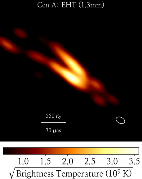
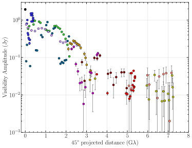
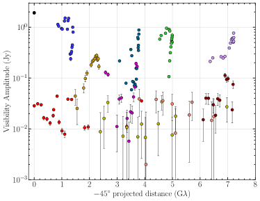
Figure 5: VLBI image reconstruction and underlying visibility amplitude data reproduced from Janssen et al. (2021). The results are from EHT observations of Centaurus A in 2017 at 228 GHz. The image shown in the left panel was reconstructed with the eht-imaging regularized maximum likelihood method. The right panel shows the visibility amplitudes as a function of $(u,v)$-distance projected along the jet direction (top) and perpendicular (bottom) to the jet direction.

When imaging VLBI data, one tries to reconstruct the sky brightness distribution that fits the data best and satisfies additional assumptions imposed to deal with the ill-posed imaging problem of incompletely sampled Fourier data from a sparse array. Strictly speaking, “imaging” refers to obtaining a pixel-based model (convolved with a resolving beam) through inverse modeling or forward modeling (Event Horizon Telescope Collaboration and et al, 2019). Inverse modeling techniques like the CLEAN algorithm (Högbom, 1974; Clark, 1980) gradually reconstruct a model in the image domain of the inverse Fourier transform of the visibilities. There are a couple of different CLEAN implementations in different software packages that are worth mentioning. The original Högbom CLEAN method (Högbom, 1974) uses iterations of delta image model components convolved with the point spread function (PSF) that are subtracted from the “dirty” image of the inverse Fourier transform. The process converges when the residual map consists only of noise. The collection of delta components form the final image model. When the residual image is added and the delta components are convolved with the VLBI resolving beam, the final image is obtained. Knowledge about interferometric images is needed to identify “false” sidelobe emission regions and to put boxes (“CLEAN windows”), which limit the locations in which CLEAN can put delta components: the emission peaks within the CLEAN windows. Clark (1980) invented a faster variant of the Högbom CLEAN for large images. Clark CLEAN operates in two cycles; the minor cycle works like the Högbom CLEAN, except that only the inner “beam patch” of the PSF is used. In major cycles, the collection of delta components are then subtracted with the full PSF. Multi-scale CLEAN (MSC, Cornwell, 2008) allows the use of extended Gaussian components for the model next to the delta components. This proved to be useful in accurately deconvolving extended / diffuse emission.

These techniques used to average the frequency bandwidth into a single channel to improve $S\,/\,N$. However, the development of multi-frequency synthesis (MFS, Conway et al., 1990; Sault and Wieringa, 1994; Likhachev, 2005) allowed the gridding of visibilities measured across multiple frequencies onto the same $(u,v)$ plane, thus improving the fidelity of the resultant image. With the widening bandwidths of modern instruments, the in-band source spectral indices limited the deconvolution accuracy when using MFS. To solve this, the multi-term multi-frequency synthesis (MT-MFS, Rau and Cornwell, 2011) algorithm models the frequency dependence of the source using a Taylor expansion. These various algorithms can be used in combination with each other depending on the observational configuration and source structures. For example, the Multi-scale multi-frequency synthesis (MS-MFS, Rau and Cornwell, 2011) combines MSC with MT-MFS.

Forward modeling techniques such as the maximum entropy method (Cornwell and Evans, 1985) fit the Fourier transform of an image to the visibility data. Additional assumptions can be incorporated as regularizers. Fitting of geometric forms such as two-dimensional Gaussian components are also done with the forward modeling approach in the visibility domain. Figure 5 shows an example VLBI image reconstruction together with the underlying visibility amplitude measurements. Projected along the jet direction, the visibility amplitudes are indicative of a smooth Gaussian-like structure. Perpendicular to the jet direction, bounding amplitudes are indicative of strong intensity gradients across the transverse jet profile.

While the VLBI scientific analysis is usually performed in the image domain, it is also possible to compare physics-based theoretical source models directly to the visibility measurements. The direct data-model comparison method will likely become more prominent in the future with the availability of increasingly advanced AGN jet models(e.g., see Mizuno, 2022, for a recent review) and machine learning methods (van der Gucht et al., 2020; Yao-Yu Lin et al., 2021). For the analysis of M87* and Sgr A* EHT observations, horizon-scale simulations (Event Horizon Telescope Collaboration and et al, 2019) are directly compared to the visibility data with (proprietary) software packages such as GENA (Fromm et al., 2019) and THEMIS (Broderick et al., 2020).

Specific combinations of the baseline-based visibilities can be formed as “closure quantities”, where station-based data errors drop out (Jennison, 1958; Blackburn et al., 2020; Broderick and Pesce, 2020; Thyagarajan et al., 2022). For example, the sum of baseline phases in a closed triangle form a robust closure phase. While uncorrected residual gain errors negatively impact reconstructed images when the full set of visibilities are utilized, with only closure quantities, one does not make use of the full information content of the data. All imaging software packages listed below (Section 5.1) are able to perform self-calibration, where, for sufficiently bright sources, within given solution intervals, per-station phase and/or amplitude gains can be found with a least-squares solver based on a comparison between the observed data and model visibilities. Typically, an initial self-calibration is performed based on a simple starting model or an initial image reconstruction where only closure quantities have been used. Subsequently, one can iteratively image and self-calibrate until the gain solutions are converged. This method of solving for the observed source structure together with calibration gains is referred to as “hybrid-mapping” (Readhead and Wilkinson, 1978; Cotton, 1979).

All imagers listed below can make use of the UVFITS visibility data format as input and produce FITS images as output. Full Stokes polarimetric imaging can be done with each imager. For details, the reader is referred to (Martí-Vidal et al., 2021, and Martí-Vidal et al., in prep.).

5.1 Software implementations

5.1.1 AIPS

The AIPS IMAGR task implements the Clark CLEAN method.

5.1.2 CASA

The CASA tclean task implements the Högbom, Clark, MSC, and MS/MT-MFS deconvolver options for CLEAN. Next to UVFITS input, the CASA imager works with its native MS visibility and metadata file format.

CASA is commonly used for spectral-line and wide-field observations, for which the corresponding special tclean features are described in Section 6.2 and Section 6.3, respectively.

5.1.3 Difmap

Difmap (Shepherd, 1997) is a widely used VLBI imaging and geometric model fitting software owing to its computational efficiency, intuitive user interface, and convenient data plotting plus flagging procedures. Difmap implements Högbom CLEAN.

5.1.4 WSClean

WSClean (Offringa et al., 2014) has been developed with the primary goal of computationally efficient wide-field imaging, for which the corresponding special software features are descried in Section 6.3. The latest version of the software can use the Clark CLEAN implementation and reconstruct MS-MFS images computationally more efficient than tclean (Offringa and Smirnov, 2017).

WSClean uses the MS file format. UVFITS input can easily be converted with the CASA importuvfits task.

5.1.5 eht-imaging

The eht-imaging software package (Chael et al., 2018, 2016) is a collection of Python modules for VLBI data analysis, with a focus on regularized maximum likelihood (RML) imaging. It includes routines for detailed mock data simulation, gain and polarimetric calibration of visibilities, image and data plotting and statistical analysis, and RML image reconstruction as well as geometric model fitting from visibilities and closure products (including full-Stokes and multi-frequency data).

5.1.6 SMILI

SMILI (Akiyama et al., 2017a, b) is a collection of sparse sampling RML forward modeling libraries, similar to eht-imaging. SMILI can be used through a Python interface.

5.1.7 UVMULTIFIT

UVMULTIFIT Martí-Vidal et al. (2014) is a flexible based geometric model fitting library that is integrated in the CASA ecosystem.

5.1.8 Comrade and DPI

The Julia-based (Bezanson et al., 2012) Comrade (Tiede et al., 2022) and Python-based Deep Probabilistic Imaging/Inference (DPI/$\alpha$-DPI, Sun et al., 2022a, b) frameworks are versatile geometric model fitting tools, which are used by the EHT (Event Horizon Telescope Collaboration and et al, 2022).

6 Advanced scientific applications

6.1 Polarization calibration

For polarization considerations, we consider the sky signal to be split into independent right-handed and left-handed circular polarizations (RCP and LCP, respectively). Such a signal split is commonly obtained in VLBI receiving systems by placing quarter-waveplates in front of linear polarization feeds. Advanced calibration methods, that have traditionally been developed for the inclusion of ALMA in VLBI experiments (Martí-Vidal et al., 2016), enable routine conversions of recorded linear polarization signals to circular ones during correlation (Section 2).

6.1.1 Additional polarization signal stabilization steps

The first step is to properly align the RCP and LCP signals. The geometric feed rotation angle evolution between the RCP and LCP data (commonly referred to as parallactic angle rotation) depends on a telescope’s focus and mount configuration (e.g., see Appendix C of Janssen et al., 2019) and is usually taken out when the data are fringe-fitted (Section 3). When all RCP and LCP fringe solutions are (re-)referenced to a common station in a stable system, a global cross-hand R-L delay will be present in the data. This is the instrumental delay between the RCP and LCP signal chains of the chosen reference station, that can be determined by fringe-fitting the RL and LR visibilities. The R-L phase is similarly affected by instrumental effects of the reference station. The true absolute R-L phase sets the orientation of the electric vector polarization angle (EVPA) of the polarized radio emission, which has to be bootstrapped from other (e.g., single-dish) observations.

If the fringe-fitting is done separately for RCP and LCP, the R-L alignment can be done as final calibration step. If polarizations are combined for the fringe-fitting, the alignment should be done as part of the instrumental calibration steps (LABEL:fig:calibrationrFlow).

6.1.2 Solving for polarization leakage effects

Subsequently, the mutual leakage of signals between the RCP and LCP signal paths at every station should be calibrated. If left uncorrected, these leakages or “$D$-terms” will impose small errors in total intensity data and add polarization signals that are purely instrumental (i.e., Stokes $\mathcal{Q}$ and $\mathcal{U}$ signals can occur for unpolarized sources). $D$-terms can have a frequency dependence, are usually stable in time, and small enough that the signal stabilization calibration does not have to be revised with leakage-corrected visibilities. Before leakages can be determined, a good image (Section 5) of the observed source is required. Firstly, to have gain errors removed by self-calibration and secondly, because solving for $D$-terms for resolved sources with complex polarization structures is not trivial (Martí-Vidal et al., 2021). For a thorough and recent overview of $D$-term calibration methods and software implementations, the reader is referred to (Martí-Vidal et al., 2021, and Martí-Vidal et al., in prep.).

6.1.3 Circular polarization

For Stokes $\mathcal{V}$ studies of VLBI data in a circular polarization basis, self-calibration solutions obtained from the RR and LL visibilities are needed to estimate the relative R/L amplitude gains of every antenna in the array. The problem is that an intrinsic Stokes $\mathcal{V}$ source polarization will confound the true residual R/L gains. A common remedy is to plan an observation where R/L gains from many observed sources based on Stokes $\mathcal{I}$ images can be obtained. Under the assumption that $\mathcal{V}=0$ on average for the sample, as there is no intrinsic preference for positive or negative intrinsic circular polarization, the mean R/L gains should be applied to the data (Homan and Wardle, 1999).

6.2 Spectral line observations

For telescopes equipped with spectrometers and a sufficient frequency resolution set at the correlator, emission and absorption features from spectral lines can be studied.

6.2.1 Spectral line signal stabilization

For spectral line observations, a few special considerations and adjustments of certain steps have to be taken into account for the signal stabilization (e.g., Goddi et al., 2004). Fringe-fit delay solutions and bandpass corrections should be obtained only on continuum sources. Depending on the reference frame used during correlation, Doppler shifts of spectral lines have to be corrected to keep the position of the line constant with respect to the correlated frequency channels after delays and the bandpass have been corrected. The center of the Earth is usually chosen as reference point during correlation and small corrections that are common for all antennas due to the Earth’s orbit around the Sun relative to the observed source are applied when shifting to the Local Standard of Rest. Such effects become increasingly relevant for longer observations. Fringe rates can be determined on the science target, selecting one or a few channels with strong line emission. Strong line emission can also be used for phase-referencing.

The AIPS and CASA fringe-fitting tasks are able to handle spectral line observations. The Doppler shifts can be corrected with the combined SETJY and CVEL tasks in AIPS and the mstransform task in CASA. The CASA imager is able to reconstruct spectral cubes (Section 5).

6.2.2 Template spectrum flux density calibration

Bright lines will show up in telescope’s auto-correlation spectra, exceeding the atmospheric noise. A template spectrum can be obtained from the measured bandpass-corrected total power response of the line from a sensitive antenna in the VLBI array. Amplitude gains in the form of time-dependent SEFDs can then be obtained without using system temperatures (Section 4) by fitting the total power spectral of all antennas to the template (Felli and Spencer, 1988, Lecture 12).

This calibration method is implemented in the AIPS task ACFIT.

6.2.3 Spectral line imaging

For spectral lines, the self-calibration is best performed with the peak line emission channel(s) image. Subsequently, spectral cube images can be made from the channels/velocities where line emission is present. If necessary, CASA tclean can perform Doppler tracking to keep the positions of spectral lines stable in the Kinematic Local Standard of Rest. For an example of a particularly extensive spectral line VLBI imaging work, the reader is referred to Matthews et al. (2010).

6.3 Wide-field VLBI

In wide-field VLBI experiments, multiple sources are observed within single pointing fields that cover the full or a signification fraction of the participating telescopes’ primary beams.

6.3.1 Wide-field correlation

For us to observe sources across the entire primary beam using VLBI, we require correlation to be conducted at a very high time (typically millisecond) and frequency ($\sim$kHz) resolutions in order to restrain smearing at the edge of the primary beam. However, the result is that a single large and often unwieldy data-set is produced which makes calibration, imaging and subsequent analysis difficult without significant computing resources. This method has been used for many of the early wide-field VLBI experiments (e.g., Chi et al., 2013) but the computational complexity and correlation resources to map the entire primary beam made wide-field VLBI observations an unattractive concept.

An alternative correlation method for wide-field VLBI was developed with the DiFX software correlator (Morgan et al., 2011) and has been implemented in the JIVE SFXC correlator (Keimpema et al., 2015). Named “multiple simultaneous phase centre observing”, this uses a two-step correlation approach. Firstly, an internal wide-field correlation produces data at the required time and frequency resolution to restrain smearing to acceptable levels at the edge of the primary beam. These data are copied and phase rotated to multiple positions across the primary beam FOV, which retains high precision astrometry as an internal geometric delay model within the correlator applies the required phase rotation. Each of these data-sets, which are centered at different positions, are then averaged to coarse time and frequency resolution, producing multiple pencil-beam data sets across the primary beam. These pencil-beams can be arranged to cover multiple sources discovered in accompanying low-resolution surveys or be mosaicked to cover a region of interest or even the whole primary beam FOV. The result from this mode of correlation is multiple small and manageable data-sets (often $\sim$GB-sized), one for each position.

6.3.2 Wide-field signal stabilization

Signal stabilization steps (Section 3) can be applied to wide-field observations as usual, by applying the calibration solutions to the data from all phase centers. Calibrator sources may be found within the phase centers as in-beam calibrators or from another area of the sky covered in a different pointing direction.

6.3.3 Wide-field imaging: primary beam correction, the $w$ term, and multi-source phase self calibration

When the beams of the participating telescopes are well determined, primary beam corrections can be employed across the FOV. For homogeneous arrays, such as the VLBA, the primary beam effectively adjusts the flux densities with distance from the pointing centre as each baseline sees the same apparent sky brightness distribution that is modified by the primary beam power envelope.

However, most VLBI arrays contain heterogeneous elements, meaning that the primary beam has significant effect even within the main lobe of the primary beam. This manifests in the data as a direction-dependent and antenna-independent gain error [see Radcliffe et. al. in prep.]. Corrections for this effect must be conducted in the $(u,v)$-plane and can be achieved in two ways. The first is to produce a direction-independent gain table with the corrections corresponding to the phase centre position (implemented through the task CLVLB in AIPS and internally within the VPIPE pipeline). This is computationally inexpensive, can account for the frequency and time dependence of the primary beam, and can be applied together with the phase-referencing corrections.

The second method is to correct during the gridding of the image reconstruction using the convolution of the complex conjugates of the primary beam voltage responses. This is more computationally complex but any residual errors are only dependent upon the accuracy of the primary beam models. Prototypes have been implemented in WSClean through the image-domain gridder (IDG) (van der Tol et al., 2018) through the application of a direction-dependent diagonal gain correction [see Radcliffe et al. in prep.].

This correction is applied together with corrections for a non-negligible $w$ term (Thompson et al., 2017) that causes increasingly larger errors in images with distance from the phase center due to sky curvature and non-coplanar baselines. Due to the $w$ term, the Fourier-transform between the visibilities and the sky brightness distribution is no longer two-dimensional. A full three-dimensional FFT would result in strong aliasing along the $w$ direction and a direct transform along $w$ is computationally too expensive for a cube that is mostly devoid of emission.

The $w$ term effects are typically corrected with one of the following methods:

• Faceting (Cornwell and Perley, 1992) performs a 2D Fourier-transform for a number of different phase centers across the FOV. The resultant pieces of image facets are small enough that the 2D FFT approximation works. The facets are stitched together and deconvolved.

• $w$-projection (Cornwell et al., 2008) uses the fact that the visibility $\mathcal{V}$ as a function of $w$ can be calculated from $\mathcal{V}$ at $w=0$ through a convolution operation: $\mathcal{V}(u,v,w)=\widetilde{G}(u,v,w)*\mathcal{V}(u,v,w=0)$. Here, $\widetilde{G}(u,v,w)$ is the Fourier transform of ${G}(u,v,w)=\exp\left[-2\pi iw\left(\sqrt{1-l^{2}-m^{2}}-1\right)\right]$. This method is faster than faceting because the visibilities need to be gridded only once.

• $w$-stacking (Offringa et al., 2014) uses a $w$-dependent grid which is FFT’ed for each gridded $w$ value and phase-shifted by ${G}^{-1}(u,v,w)$. For imaging, all grids are summed with appropriate scaling factors (see Offringa et al., 2014, for details). Compared to $w$-projection, $w$-stacking is faster when the visibility gridding is computationally more expensive than the FFT computations.

WSClean implements the $w$-stacking method and tclean implements the $w$-projection algorithm and can do faceting.

The phase stability of VLBI arrays is worse than connected short-baseline arrays due to the differing atmospheric paths between antenna and source. This means that self-calibration (Section 5) is essential in achieving low noise and high dynamic ranges. Self-calibration requires a source with sufficient S/N to estimate the gain corrections along the line-of-sight to the target field. However, for VLBI observations, its lack of sensitivity to large scale, diffuse emission means that the total flux available for self-calibration of a single source can be insufficient, restricting VLBI observations to those fields with in-beam, or nearby phase calibrators.

However, for wide-field VLBI, the targeting of multiple sources allows self-calibration to proceed, even when each individual target is faint, by using the combined flux density of the detected sources (Middelberg et al., 2013; Radcliffe et al., 2016). This technique, called “multi-source self-calibration”, images each source detected after phase referencing and divides the visibilities are divided by the model to produce a point source at the phase centre. These data sets are stacked in the $(u,v)$-plane and self-calibration solutions obtained using the combined S/N of all target sources. This technique is currently being developed into a fully directional-dependent technique through the derivation of self-calibration solutions along different line-of-sights across the primary beam [Harth et al. in prep.].

7 Synthetic data

Forward-modeling methods, where the $(u,v)$-coverage, thermal noise and simple telescope gain errors are taken into account to create simulated/fake visibility data based on a model sky brightness distribution, have been available for a while (e.g., the DTSIM AIPS task, simobserve in CASA, and MeqTrees (Noordam and Smirnov, 2010)). Recently, very accurate visibility simulations have been developed: The data simulation toolkit within eht-imaging and the SYnthetic Measurement creator for long Baseline Arrays (SYMBA) (Roelofs et al., 2020). Both methods make use of sophisticated data corruption models, are able to include the effects of interstellar scattering, can use arbitrary source models defined in text files or images from HDF5 and FITS data, and use the exact $(u,v)$-coverage from (observational) UVFITS input. SYMBA and eht-imaging are routinely used by the EHT to generating synthetic data for dedicated tests to answer specific scientific questions (e.g., about the robustness of specific features in reconstructed images), optimize calibration procedures, produce imaging parameter surveys, create test suites for software packages, and identify how to optimally upgrade VLBI arrays (e.g., Event Horizon Telescope Collaboration and et al., 2019; Event Horizon Telescope Collaboration and et al, 2019, 2019; Wielgus et al., 2020; Roelofs et al., 2021; Janssen et al., 2021).

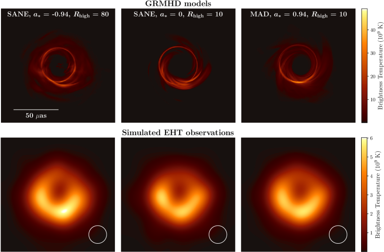
Figure 6: Synthetic EHT observations of M87*. Top: Ray-traced GRMHD simulations (Event Horizon Telescope Collaboration et al., 2019) from the EHT library with different black hole spins, electron temperature parameters, and magnetic field states (“MAD” versus “SANE”). Bottom: SYMBA synthetic observations corresponding to these models. Reproduced from Event Horizon Telescope Collaboration and et al. (2019).

The versatile eht-imaging package bootstraps data corruption effects from a calibrated UVFITS file of observational data and produces a UVFITS output. The CASA-based SYMBA software produces both UVFITS and MS output. Data corruptions effects are simulated from first principles with MeqSilhouette to emulate the correlator output in a real observation (Blecher et al., 2017; Natarajan et al., 2022). For example, physical parameters for atmospheric or antenna-pointing models can be adjusted and their effects studied. The suite of possible MeqSilhouette data corruption effects is continuously being expanded; Faraday rotation effects from the interstellar medium and atmospheric effects from the ionosphere will soon be added for example. SYMBA passes the MeqSilhouette output to rPICARD, which results in science-ready calibrated synthetic data akin to that from a real observation. Work is ongoing to convert SYMBA to simulate low frequency VLBI and enable feasability studies of new instruments such as SKA-VLBI.

The ability to simulate VLBI data based on known ground-truth models allow non-experts to better understand the fundamentals of VLBI data. For example, by looking at the amplitude and phase signatures of simple geometric models or by studying how specific calibration errors manifest themselves in the data. Examples of synthetic EHT observations based on state-of-the-art theoretical models are shown in Figure 6.

Next to the full forward-modeling software packages, there are also dedicated VLBI observing simulators, such as the Very long baseline interferometry Network SIMulator (VNSIM) (Zhao et al., 2019). These tools assist users and engineers with the design and scheduling of VLBI experiments, as well as the evaluation of the array performance under various conditions.

8 Summary

In this work we have presented current open-source VLBI methods and their implementations in various software. LABEL:tab:softwares provides and overview of the major software packages’ capabilities. Several of these packages can be easily obtained through the KERN repository (Molenaar and Smirnov, 2018) alongside many additional radio astronomical software libraries.

Table 2: Major VLBI software packages and their capabilities. AIPS and Difmap are still supported by their originators; requested features and bug fixes can be implemented. All other packages are actively being developed and supported by larger communities and institutions.

Name	Capabilities	Links and references
DiFX	Correlation	https://ascl.net/1102.024,   https://svn.atnf.csiro.au/difx,  Deller et al. (2007, 2011)
SFXC	Correlation	https://svn.astron.nl/sfxc,  Keimpema et al. (2015)
AIPS, ParselTongue	Signal stabilization, flux density calibration, imaging, synthetic data generation	https://ascl.net/9911.003,  https://ascl.net/1208.020, http://www.aips.nrao.edu,   https://www.jive.eu/jivewiki/doku.php?id=parseltongue:parseltongue,  (Greisen, 2003; Kettenis et al., 2006)
CASA  - VPIPE  - rPICARD	Signal stabilization, flux density calibration, imaging	https://ascl.net/1107.013,  https://casa.nrao.edu   https://github.com/jradcliffe5/VLBI_pipeline https://ascl.net/1905.015,   https://bitbucket.org/M_Janssen/picard,   https://hub.docker.com/r/mjanssen2308/casavlbi,   McMullin et al. (2007); Janssen et al. (2018, 2019)
(EHT-)HOPS	Signal stabilization, flux denisity calibration	https://www.haystack.mit.edu/tech/vlbi/hops.html, https://github.com/sao-eht/eat,  Whitney et al. (2004); Blackburn et al. (2019)
Difmap	Imaging, model fitting	https://ascl.net/1103.001,   ftp://ftp.astro.caltech.edu/pub/difmap/difmap.html,  (Shepherd, 1997)
eht-imaging	Imaging, model fitting, synthetic data generation	https://ascl.net/1904.004,   https://github.com/achael/eht-imaging,  (Chael et al., 2018, 2016)
SMILI	Imaging	https://ascl.net/1904.005,   https://github.com/astrosmili/smili,  (Akiyama et al., 2017a, b)
WSClean	Imaging	https://ascl.net/1408.023,   https://gitlab.com/aroffringa/wsclean,  (Offringa et al., 2014)
UV- MULTIFIT	Geometric model fitting	https://ascl.net/1402.017,   https://launchpad.net/uvmultifit,  (Martí-Vidal et al., 2014)
SYMBA	Synthetic data generation	https://bitbucket.org/M_Janssen/symba,  (Roelofs et al., 2020)

Appendix A Telescope baseband data transport to the VLBI correlator

Baseband data from all stations need to be available simultaneously for correlation. One option is real-time streaming to the VLBI correlator. This is an observing mode in e-MERLIN (Davies et al., 1980), e-EVN, and future VLBA after ongoing upgrades.

Real-time correlation is possible if the network paths from the VLBI telescopes (connected at typically 1G/10G/100G) to the correlator (typically 10G/100G) offer sufficient capacity and can maintain real-time rates reliably with an acceptably low data loss fraction. On paths that cross the Internet this can be challenging. A drawback is also that re-correlations with different settings are not possible, unless the baseband data are stored.

In most VLBI experiments the baseband data are captured at the telescopes onto a recorder such as FlexBuff, Mark 6, or Octadisk2. The recording media can be physically shipped by courier mail. The proprietary form factor of the media requires a corresponding playback unit at the correlator.

Alternatively, baseband data files can be transferred at slower pace over the Internet to the correlator. Popular high speed data transfer software for this purpose are JIVE jive5ab and etc/etd, Tsunami UDP transfer, and Globus GridFTP. Transfer with slower scp or rsync is also used as a fallback. In an “e-shipping” mode, the transferred data are stored on a cluster or cloud file system until later correlation. In contrast, real-time correlation of the transferred data is commonly referred to as “e-VLBI”.

Appendix B Data flagging

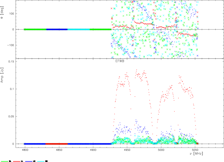
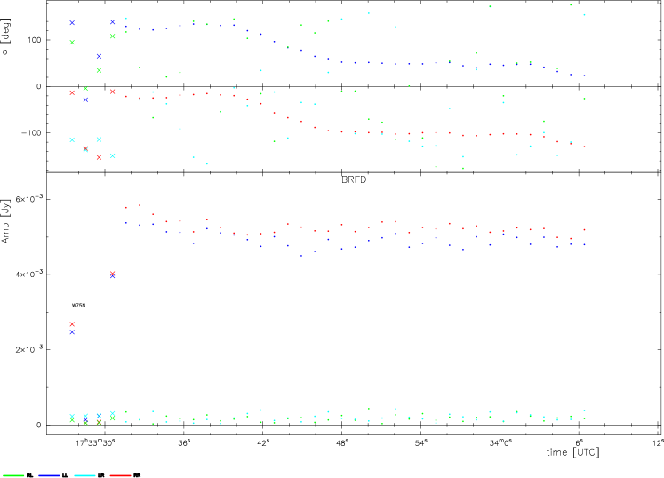
Figure 7: Examples of flagged bad data indicated with crosses. These plots are produced automatically with jiveplot by rPICARD and show visibility amplitudes and phases per baseline and per scan, color-coded by polarization. Top: Scan-averaged EVN data on the Effelsberg-Westerbork baseline. The Effelsberg RCP channel and first four spectral windows contain no signal and have been flagged. Bottom: Frequency-averaged VLBA data on the Brewster-Hancock baseline. Brewster has been a few seconds late on source, resulting in bad phases and amplitudes at the start of the scan.

The flagging (removal) of “bad data” is common practice in interferometry. With enough antennas in the array, one can be rather liberal with the data flagging. VLBI arrays, however, are often sparse. Care must be taken to distinguish bad data from correctable calibration errors and measurements with low $S\,/\,N$. Common uncorrectable problems are issues along the telescope data recoding path that may render data at specific frequency channels or polarizations unusable, telescopes that are late on source or experience severe weather, bandpass fall-offs (“frequency edge-channels”), and RFI. In the unaveraged data, baseline-based problems are rare and the flagging should be done on a per-antenna basis. There are some algorithms that can automatically identify some bad data, e.g., for RFI (Offringa et al., 2012), but to the authors’ knowledge there is no software that is fully sufficient for VLBI data. The VLBI data flagging therefore remains a subjective task.

Flags are usually applied at different data reduction stages. A priori flags based on telescope operator logs are made available to PIs. Low $S\,/\,N$ fringe non-detections render the underlying data flagged, but care must be taken here as the fringe-fitting segmentation time does not necessarily match the time ranges over which data issues are present. Partially affected data over VLBI scan durations should be removed before fringe-fitting. Finally, manifestations of bad data and calibration errors can easily be identified in image reconstructions as spurious features. Figure 7 shows two typical examples of bad data that should be flagged.

References yes

References

- Gaylard et al. (2011) Gaylard, M.J.; Bietenholz, M.F.; Combrinck, L.; Booth, R.S.; Buchner, S.J.; Fanaroff, B.L.; MacLeod, G.C.; Nicolson, G.D.; Quick, J.F.H.; Stronkhorst, P.; Venkatasubramani, T.L. An African VLBI Network of radio telescopes. Proceedings of SAIP2011, 2011, pp. 473–478, [arXiv:astro-ph.IM/1405.7214].
- Deane (2016) Deane, R. Extragalactic VLBI surveys in the MeerKAT era. MeerKAT Science: On the Pathway to the SKA, 2016, p. 17, [arXiv:astro-ph.IM/1709.03512].
- Matthews et al. (2018) Matthews, L.D.; Crew, G.B.; Doeleman, S.S.; et al. The ALMA Phasing System: A Beamforming Capability for Ultra-high-resolution Science at (Sub)Millimeter Wavelengths. PASP 2018, 130, 015002, [arXiv:astro-ph.IM/1711.06770].
- Venturi et al. (2020) Venturi, T.; Paragi, Z.; Lindqvist, M.; et al. VLBI20-30: a scientific roadmap for the next decade – The future of the European VLBI Network. arXiv e-prints 2020, p. arXiv:2007.02347, [arXiv:astro-ph.IM/2007.02347].
- Barbosa et al. (2021) Barbosa, D.; Coelho, B.; Antón, S.; Bergano, M.; Boekholt, T.; Correia, A.C.M.; Maia, D.; Pandeirada, J.; Ribeiro, V.; Adams, J.; Barraca, J.P.; Gomes, D.; Morgado, B. Radio astronomy and Space science in Azores: Enhancing the Atlantic VLBI infrastructure cluster. Advances in Space Research 2021, 68, 3064–3078, [arXiv:astro-ph.IM/2107.03437].
- Whitney et al. (2013) Whitney, A.R.; Beaudoin, C.J.; Cappallo, R.J.; Corey, B.E.; Crew, G.B.; Doeleman, S.S.; Lapsley, D.E.; Hinton, A.A.; McWhirter, S.R.; Niell, A.E.; Rogers, A.E.E.; Ruszczyk, C.A.; Smythe, D.L.; SooHoo, J.; Titus, M.A. Demonstration of a 16 Gbps Station-1 Broadband-RF VLBI System. PASP 2013, 125, 196.
- Vertatschitsch et al. (2015) Vertatschitsch, L.; Primiani, R.; Young, A.; Weintroub, J.; Crew, G.B.; McWhirter, S.R.; Beaudoin, C.; Doeleman, S.; Blackburn, L. R2DBE: A Wideband Digital Backend for the Event Horizon Telescope. PASP 2015, 127, 1226.
- Han et al. (2008) Han, S.T.; Lee, J.W.; Kang, J.; Je, D.H.; Chung, M.H.; Wi, S.O.; Sasao, T.; Wylde, R. Millimeter-wave Receiver Optics for Korean VLBI Network. International Journal of Infrared and Millimeter Waves 2008, 29, 69–78.
- Boccardi et al. (2017) Boccardi, B.; Krichbaum, T.P.; Ros, E.; Zensus, J.A. Radio observations of active galactic nuclei with mm-VLBI. A&A Rev. 2017, 25, 4, [arXiv:astro-ph.HE/1711.07548].
- Event Horizon Telescope Collaboration and et al. (2019) Event Horizon Telescope Collaboration.; et al.. First M87 Event Horizon Telescope Results. I. The Shadow of the Supermassive Black Hole. ApJ 2019, 875, L1, [arXiv:astro-ph.GA/1906.11238].
- Selina et al. (2018) Selina, R.J.; Murphy, E.J.; McKinnon, M.; Beasley, A.; Butler, B.; Carilli, C.; Clark, B.; Durand, S.; Erickson, A.; Grammer, W.; Hiriart, R.; Jackson, J.; Kent, B.; Mason, B.; Morgan, M.; Ojeda, O.Y.; Rosero, V.; Shillue, W.; Sturgis, S.; Urbain, D. The ngVLA Reference Design. Science with a Next Generation Very Large Array; Murphy, E., Ed., 2018, Vol. 517, Astronomical Society of the Pacific Conference Series, p. 15, [arXiv:astro-ph.IM/1810.08197].
- Murphy et al. (2018) Murphy, E.J.; Bolatto, A.; Chatterjee, S.; Casey, C.M.; Chomiuk, L.; Dale, D.; de Pater, I.; Dickinson, M.; Francesco, J.D.; Hallinan, G.; Isella, A.; Kohno, K.; Kulkarni, S.R.; Lang, C.; Lazio, T.J.W.; Leroy, A.K.; Loinard, L.; Maccarone, T.J.; Matthews, B.C.; Osten, R.A.; Reid, M.J.; Riechers, D.; Sakai, N.; Walter, F.; Wilner, D. The ngVLA Science Case and Associated Science Requirements. Science with a Next Generation Very Large Array; Murphy, E., Ed., 2018, Vol. 517, Astronomical Society of the Pacific Conference Series, p. 3, [arXiv:astro-ph.IM/1810.07524].
- Dewdney et al. (2009) Dewdney, P.E.; Hall, P.J.; Schilizzi, R.T.; Lazio, T.J.L.W. The Square Kilometre Array. IEEE Proceedings 2009, 97, 1482–1496.
- Paragi et al. (2015) Paragi, Z.; Godfrey, L.; Reynolds, C.; et al. Very Long Baseline Interferometry with the SKA. Advancing Astrophysics with the Square Kilometre Array (AASKA14), 2015, p. 143, [arXiv:astro-ph.IM/1412.5971].
- Doeleman et al. (2019) Doeleman, S.; Blackburn, L.; Dexter, J.; et al. Studying Black Holes on Horizon Scales with VLBI Ground Arrays. Bulletin of the American Astronomical Society, 2019, Vol. 51, p. 256, [arXiv:astro-ph.IM/1909.01411].
- Kardashev et al. (2014) Kardashev, N.S.; Novikov, I.D.; Lukash, V.N.; Pilipenko, S.V.; Mikheeva, E.V.; Bisikalo, D.V.; Wiebe, D.S.; Doroshkevich, A.G.; Zasov, A.V.; Zinchenko, I.I.; Ivanov, P.B.; Kostenko, V.I.; Larchenkova, T.I.; Likhachev, S.F.; Malov, I.F.; Malofeev, V.M.; Pozanenko, A.S.; Smirnov, A.V.; Sobolev, A.M.; Cherepashchuk, A.M.; Shchekinov, Y.A. Review of scientific topics for the Millimetron space observatory. Physics Uspekhi 2014, 57, 1199–1228, [arXiv:astro-ph.IM/1502.06071].
- Johnson et al. (2019) Johnson, M.; Haworth, K.; Pesce, D.W.; Palumbo, D.C.M.; Blackburn, L.; Akiyama, K.; Boroson, D.; Bouman, K.L.; Farah, J.R.; Fish, V.L.; Honma, M.; Kawashima, T.; Kino, M.; Raymond, A.; Silver, M.; Weintroub, J.; Wielgus, M.; Doeleman, S.S.; Kauffmann, J.; Keating, G.K.; Krichbaum, T.P.; Loinard, L.; Narayanan, G.; Doi, A.; James, D.J.; Marrone, D.P.; Mizuno, Y.; Nagai, H. Studying black holes on horizon scales with space-VLBI. Bulletin of the American Astronomical Society, 2019, Vol. 51, p. 235, [arXiv:astro-ph.IM/1909.01405].
- Fish et al. (2020) Fish, V.L.; Shea, M.; Akiyama, K. Imaging black holes and jets with a VLBI array including multiple space-based telescopes. Advances in Space Research 2020, 65, 821–830, [arXiv:astro-ph.IM/1903.09539].
- Gurvits et al. (2021) Gurvits, L.I.; Paragi, Z.; Casasola, V.; Conway, J.; Davelaar, J.; Falcke, H.; Fender, R.; Frey, S.; Fromm, C.M.; Miró, C.G.; Garrett, M.A.; Giroletti, M.; Goddi, C.; Gómez, J.L.; van der Gucht, J.; Guirado, J.C.; Haiman, Z.; Helmich, F.; Humphreys, E.; Impellizzeri, V.; Kramer, M.; Lindqvist, M.; Linz, H.; Liuzzo, E.; Lobanov, A.P.; Mizuno, Y.; Rezzolla, L.; Roelofs, F.; Ros, E.; Rygl, K.L.J.; Savolainen, T.; Schuster, K.; Venturi, T.; Wiedner, M.C.; Zensus, J.A. THEZA: TeraHertz Exploration and Zooming-in for Astrophysics. Experimental Astronomy 2021, 51, 559–594, [arXiv:astro-ph.IM/1908.10767].
- Marcote et al. (2017) Marcote, B.; Paragi, Z.; Hessels, J.W.T.; Keimpema, A.; van Langevelde, H.J.; Huang, Y.; Bassa, C.G.; Bogdanov, S.; Bower, G.C.; Burke-Spolaor, S.; Butler, B.J.; Campbell, R.M.; Chatterjee, S.; Cordes, J.M.; Demorest, P.; Garrett, M.A.; Ghosh, T.; Kaspi, V.M.; Law, C.J.; Lazio, T.J.W.; McLaughlin, M.A.; Ransom, S.M.; Salter, C.J.; Scholz, P.; Seymour, A.; Siemion, A.; Spitler, L.G.; Tendulkar, S.P.; Wharton, R.S. The Repeating Fast Radio Burst FRB 121102 as Seen on Milliarcsecond Angular Scales. ApJ 2017, 834, L8, [arXiv:astro-ph.HE/1701.01099].
- Event Horizon Telescope Collaboration and et al (2022) Event Horizon Telescope Collaboration.; et al. First Sagittarius A* Event Horizon Telescope Results. I. The Shadow of the Supermassive Black Hole in the Center of the Milky Way. ApJ 2022, 930, L12.
- Gabuzda (2018) Gabuzda, D. Evidence for Helical Magnetic Fields Associated with AGN Jets and the Action of a Cosmic Battery. Galaxies 2018, 7, 5.
- Gabuzda (2020) Gabuzda, D.C. Polarization VLBI observations of AGN jets now and into the future. Advances in Space Research 2020, 65, 731–738.
- Event Horizon Telescope Collaboration and et al (2021a) Event Horizon Telescope Collaboration.; et al. First M87 Event Horizon Telescope Results. VII. Polarization of the Ring. ApJ 2021, 910, L12, [arXiv:astro-ph.HE/2105.01169].
- Event Horizon Telescope Collaboration and et al (2021b) Event Horizon Telescope Collaboration.; et al. First M87 Event Horizon Telescope Results. VIII. Magnetic Field Structure near The Event Horizon. ApJ 2021, 910, L13, [arXiv:astro-ph.HE/2105.01173].
- Gabuzda (2021) Gabuzda, D.C. Inherent and Local Magnetic Field Structures in Jets from Active Galactic Nuclei. Galaxies 2021, 9, 58.
- Habing (1996) Habing, H.J. Circumstellar envelopes and Asymptotic Giant Branch stars. A&A Rev. 1996, 7, 97–207.
- Momjian et al. (2003) Momjian, E.; Romney, J.D.; Carilli, C.L.; Troland, T.H. Sensitive VLBI Continuum and H I Absorption Observations of NGC 7674: First Scientific Observations with the Combined Array VLBA, VLA, and Arecibo. ApJ 2003, 597, 809–822, [arXiv:astro-ph/astro-ph/0307399].
- Goddi et al. (2005) Goddi, C.; Moscadelli, L.; Alef, W.; Tarchi, A.; Brand, J.; Pani, M. Kinematics of H2O masers in high-mass star forming regions. A&A 2005, 432, 161–173, [arXiv:astro-ph/astro-ph/0411164].
- Hachisuka et al. (2006) Hachisuka, K.; Brunthaler, A.; Menten, K.M.; Reid, M.J.; Imai, H.; Hagiwara, Y.; Miyoshi, M.; Horiuchi, S.; Sasao, T. Water Maser Motions in W3(OH) and a Determination of Its Distance. ApJ 2006, 645, 337–344, [arXiv:astro-ph/astro-ph/0512226].
- Reid et al. (2009) Reid, M.J.; Braatz, J.A.; Condon, J.J.; Greenhill, L.J.; Henkel, C.; Lo, K.Y. The Megamaser Cosmology Project. I. Very Long Baseline Interferometric Observations of UGC 3789. ApJ 2009, 695, 287–291, [arXiv:astro-ph/0811.4345].
- Brunthaler et al. (2011) Brunthaler, A.; Reid, M.J.; Menten, K.M.; Zheng, X.W.; Bartkiewicz, A.; Choi, Y.K.; Dame, T.; Hachisuka, K.; Immer, K.; Moellenbrock, G.; Moscadelli, L.; Rygl, K.L.J.; Sanna, A.; Sato, M.; Wu, Y.; Xu, Y.; Zhang, B. The Bar and Spiral Structure Legacy (BeSSeL) survey: Mapping the Milky Way with VLBI astrometry. Astronomische Nachrichten 2011, 332, 461, [arXiv:astro-ph.GA/1102.5350].
- Goddi et al. (2011) Goddi, C.; Moscadelli, L.; Sanna, A. Infall and outflow within 400 AU from a high-mass protostar. 3D velocity fields from methanol and water masers in AFLG 5142. A&A 2011, 535, L8, [arXiv:astro-ph.GA/1110.1647].
- Reid et al. (2013) Reid, M.J.; Braatz, J.A.; Condon, J.J.; Lo, K.Y.; Kuo, C.Y.; Impellizzeri, C.M.V.; Henkel, C. The Megamaser Cosmology Project. IV. A Direct Measurement of the Hubble Constant from UGC 3789. ApJ 2013, 767, 154, [arXiv:astro-ph.CO/1207.7292].
- Goddi et al. (2017) Goddi, C.; Surcis, G.; Moscadelli, L.; Imai, H.; Vlemmings, W.H.T.; van Langevelde, H.J.; Sanna, A. Measuring magnetic fields from water masers in the synchrotron protostellar jet in W3(H2O). A&A 2017, 597, A43, [arXiv:astro-ph.GA/1608.02951].
- Moscadelli et al. (2019) Moscadelli, L.; Sanna, A.; Goddi, C.; Krishnan, V.; Massi, F.; Bacciotti, F. Protostellar Outflows at the EarliesT Stages (POETS). III. H2O masers tracing disk-winds and jets near luminous YSOs. A&A 2019, 631, A74, [arXiv:astro-ph.SR/1909.08374].
- Garrett et al. (2001) Garrett, M.A.; Muxlow, T.W.B.; Garrington, S.T.; Alef, W.; Alberdi, A.; van Langevelde, H.J.; Venturi, T.; Polatidis, A.G.; Kellermann, K.I.; Baan, W.A.; Kus, A.; Wilkinson, P.N.; Richards, A.M.S. AGN and starbursts at high redshift: High resolution EVN radio observations of the Hubble Deep Field. A&A 2001, 366, L5–L8, [arXiv:astro-ph/astro-ph/0102037].
- Herrera Ruiz et al. (2017) Herrera Ruiz, N.; Middelberg, E.; Deller, A.; Norris, R.P.; Best, P.N.; Brisken, W.; Schinnerer, E.; Smolčić, V.; Delvecchio, I.; Momjian, E.; Bomans, D.; Scoville, N.Z.; Carilli, C. The faint radio sky: VLBA observations of the COSMOS field. A&A 2017, 607, A132, [arXiv:astro-ph.GA/1707.07512].
- Radcliffe et al. (2018) Radcliffe, J.F.; Garrett, M.A.; Muxlow, T.W.B.; Beswick, R.J.; Barthel, P.D.; Deller, A.T.; Keimpema, A.; Campbell, R.M.; Wrigley, N. Nowhere to Hide: Radio-faint AGN in GOODS-N field. I. Initial catalogue and radio properties. A&A 2018, 619, A48, [arXiv:astro-ph.GA/1808.04296].
- Spingola et al. (2018) Spingola, C.; Mckean, J.P.; Deller, A.; Moldon, J. Gravitational lensing at milliarcsecond angular resolution with VLBI observations. 14th European VLBI Network Symposium & Users Meeting (EVN 2018), 2018, p. 33, [arXiv:astro-ph.GA/1902.07046].
- Spingola et al. (2019) Spingola, C.; McKean, J.P.; Lee, M.; Deller, A.; Moldon, J. A novel search for gravitationally lensed radio sources in wide-field VLBI imaging from the mJIVE-20 survey. MNRAS 2019, 483, 2125–2153, [arXiv:astro-ph.GA/1811.09152].
- Deller et al. (2019) Deller, A.T.; Goss, W.M.; Brisken, W.F.; Chatterjee, S.; Cordes, J.M.; Janssen, G.H.; Kovalev, Y.Y.; Lazio, T.J.W.; Petrov, L.; Stappers, B.W.; Lyne, A. Microarcsecond VLBI Pulsar Astrometry with PSR II. Parallax Distances for 57 Pulsars. ApJ 2019, 875, 100, [arXiv:astro-ph.IM/1808.09046].
- Duev et al. (2012) Duev, D.A.; Molera Calvés, G.; Pogrebenko, S.V.; Gurvits, L.I.; Cimó, G.; Bocanegra Bahamon, T. Spacecraft VLBI and Doppler tracking: algorithms and implementation. A&A 2012, 541, A43, [arXiv:astro-ph.IM/1203.4408].
- Thompson et al. (2017) Thompson, A.R.; Moran, J.M.; Swenson, Jr., G.W. Interferometry and Synthesis in Radio Astronomy, 3rd Edition; Springer International Publishing, 2017.
- Morabito et al. (2022) Morabito, L.K.; Jackson, N.J.; Mooney, S.; et al. Sub-arcsecond imaging with the International LOFAR Telescope. I. Foundational calibration strategy and pipeline. A&A 2022, 658, A1, [arXiv:astro-ph.IM/2108.07283].
- Allan (1966) Allan, D.W. Statistics of atomic frequency standards. IEEE Proceedings 1966, 54, 221–230.
- Primiani et al. (2016) Primiani, R.A.; Young, K.H.; Young, A.; Patel, N.; Wilson, R.W.; Vertatschitsch, L.; Chitwood, B.B.; Srinivasan, R.; MacMahon, D.; Weintroub, J. SWARM: A 32 GHz Correlator and VLBI Beamformer for the Submillimeter Array. Journal of Astronomical Instrumentation 2016, 5, 1641006–810, [arXiv:astro-ph.IM/1611.02596].
- Kim et al. (2004) Kim, H.G.; Han, S.T.; Sohn, B.W.; Oh, S.J.; Je, D.H.; Wi, S.O.; Song, M.G. Construction of the Korean VLBI Network (KVN). European VLBI Network on New Developments in VLBI Science and Technology, 2004, pp. 281–284, [arXiv:astro-ph/astro-ph/0412689].
- Lee et al. (2011) Lee, S.S.; Byun, D.Y.; Oh, C.S.; Han, S.T.; Je, D.H.; Kim, K.T.; Wi, S.O.; Cho, S.H.; Sohn, B.W.; Kim, J.; Lee, J.; Oh, S.J.; Song, M.G.; Kang, J.; Chung, M.H.; Lee, J.A.; Oh, J.; Bae, J.H.; Yun, S.Y.; Lee, J.W.; Kim, B.G.; Chung, H.; Roh, D.G.; Lee, C.H.; Kim, H.G.; Ryoung Kim, H.; Yeom, J.H.; Kurayama, T.; Jung, T.; Park, P.; Kim, M.J.; Yoon, D.H.; Kim, W.J. Single-Dish Performance of KVN 21 m Radio Telescopes: Simultaneous Observations at 22 and 43 GHz. PASP 2011, 123, 1398, [arXiv:astro-ph.IM/1110.3881].
- Lee et al. (2014) Lee, S.S.; Petrov, L.; Byun, D.Y.; Kim, J.; Jung, T.; Song, M.G.; Oh, C.S.; Roh, D.G.; Je, D.H.; Wi, S.O.; Sohn, B.W.; Oh, S.J.; Kim, K.T.; Yeom, J.H.; Chung, M.H.; Kang, J.; Han, S.T.; Lee, J.W.; Kim, B.G.; Chung, H.; Kim, H.G.; Ryoung Kim, H.; Kang, Y.W.; Cho, S.H. Early Science with the Korean VLBI Network: Evaluation of System Performance. AJ 2014, 147, 77.
- Kobayashi et al. (2003) Kobayashi, H.; Sasao, T.; Kawaguchi, N.; Manabe, S.; Omodaka, T.; Kameya, O.; Shibata, K.M.; Miyaji, T.; Honma, M.; Tamura, Y.; Hirota, T.; Kuji, S.; Horiai, K.; Sakai, S.; Sato, K.; Iwadate, K.; Kanya, Y.; Ujihara, H.; Jike, T.; Fujii, T.; Motiduki, N.; Oyama, T.; Kurayama, H.; Kamohara, R.; Suda, H.; Kasuga, T. VERA: A New VLBI Instrument Free from the Atmosphere. New technologies in VLBI; Minh, Y.C., Ed., 2003, Vol. 306, Astronomical Society of the Pacific Conference Series, p. 367.
- Lee et al. (2015) Lee, S.S.; Oh, C.S.; Roh, D.G.; Oh, S.J.; Kim, J.; Yeom, J.H.; Kim, H.R.; Jung, D.G.; Byun, D.Y.; Jung, T.; Kawaguchi, N.; Shibata, K.M.; Wajima, K. A New Hardware Correlator in Korea: Performance Evaluation Using KVN Observations. Journal of Korean Astronomical Society 2015, 48, 125–137, [arXiv:astro-ph.IM/1503.07972].
- Deller et al. (2007) Deller, A.T.; Tingay, S.J.; Bailes, M.; West, C. DiFX: A Software Correlator for Very Long Baseline Interferometry Using Multiprocessor Computing Environments. PASP 2007, 119, 318–336, [arXiv:astro-ph/astro-ph/0702141].
- Deller et al. (2011) Deller, A.T.; Brisken, W.F.; Phillips, C.J.; Morgan, J.; Alef, W.; Cappallo, R.; Middelberg, E.; Romney, J.; Rottmann, H.; Tingay, S.J.; Wayth, R. DiFX-2: A More Flexible, Efficient, Robust, and Powerful Software Correlator. PASP 2011, 123, 275, [arXiv:astro-ph.IM/1101.0885].
- Keimpema et al. (2015) Keimpema, A.; Kettenis, M.M.; Pogrebenko, S.V.; Campbell, R.M.; Cimó, G.; Duev, D.A.; Eldering, B.; Kruithof, N.; van Langevelde, H.J.; Marchal, D.; Molera Calvés, G.; Ozdemir, H.; Paragi, Z.; Pidopryhora, Y.; Szomoru, A.; Yang, J. The SFXC software correlator for very long baseline interferometry: algorithms and implementation. Experimental Astronomy 2015, 39, 259–279, [arXiv:astro-ph.IM/1502.00467].
- Napier et al. (1994) Napier, P.J.; Bagri, D.S.; Clark, B.G.; Rogers, A.E.E.; Romney, J.D.; Thompson, A.R.; Walker, R.C. The Very Long Baseline Array. IEEE Proceedings 1994, 82, 658–672.
- Event Horizon Telescope Collaboration and et al (2019) Event Horizon Telescope Collaboration.; et al. First M87 Event Horizon Telescope Results. II. Array and Instrumentation. ApJ 2019, 875, L2, [arXiv:astro-ph.IM/1906.11239].
- Porcas (2010) Porcas, R. A history of the EVN. 10th European VLBI Network Symposium and EVN Users Meeting: VLBI and the New Generation of Radio Arrays, 2010, Vol. 10, p. 11.
- Surkis et al. (2017) Surkis, I.; Ken, V.; Kurdubova, Y.; Mishina, N.; Mishin, V.; Shantyr, V.; Zhuravov, D.; Zimovsky, V. The RASFX VGOS GPU Based Software Correlator. Transactions of the Institute of Applied Astronomy RAS 2017, pp. 123–126.
- Shuygina et al. (2019) Shuygina, N.; Ivanov, D.; Ipatov, A.; Gayazov, I.; Marshalov, D.; Melnikov, A.; Kurdubov, S.; Vasilyev, M.; Ilin, G.; Skurikhina, E.; Surkis, I.; Mardyshkin, V.; Mikhailov, A.; Salnikov, A.; Vytnov, A.; Rakhimov, I.; Dyakov, A.; Olifirov, V. Russian VLBI network “Quasar”: Current status and outlook. Geodesy and Geodynamics 2019, 10, 150–156. From Space Geodesy to Astro-Geodynamics.
- Zhang et al. (2021) Zhang, F.; Zhao, C.; Han, S.; Ma, F.; Xiang, D. GPU-Based Parallel Implementation of VLBI Correlator for Deep Space Exploration System. Remote Sensing 2021, 13, 1226.
- Rioja et al. (2012) Rioja, M.; Dodson, R.; Asaki, Y.; Hartnett, J.; Tingay, S. The Impact of Frequency Standards on Coherence in VLBI at the Highest Frequencies. AJ 2012, 144, 121, [arXiv:astro-ph.IM/1209.3989].
- Clivati et al. (2020) Clivati, C.; Aiello, R.; Bianco, G.; Bortolotti, C.; De Natale, P.; Di Sarno, V.; Maddaloni, P.; Maccaferri, G.; Mura, A.; Negusini, M.; Levi, F.; Perini, F.; Ricci, R.; Roma, M.; Amato, L.S.; de Cumis, M.S.; Stagni, M.; Tuozzi, A.; Calonico, D. Common-clock very long baseline interferometry using a coherent optical fiber link. Optica 2020, 7, 1031–1037.
- Krehlik et al. (2017) Krehlik, P.; Buczek, Ł.; Kołodziej, J.; Lipiński, M.; Śliwczyński, Ł.; Nawrocki, J.; Nogaś, P.; Marecki, A.; Pazderski, E.; Ablewski, P.; Bober, M.; Ciuryło, R.; Cygan, A.; Lisak, D.; Masłowski, P.; Morzyński, P.; Zawada, M.; Campbell, R.M.; Pieczerak, J.; Binczewski, A.; Turza, K. Fibre-optic delivery of time and frequency to VLBI station. A&A 2017, 603, A48, [arXiv:astro-ph.IM/1703.09479].
- Likhachev et al. (2017) Likhachev, S.F.; Kostenko, V.I.; Girin, I.A.; Andrianov, A.S.; Rudnitskiy, A.G.; Zharov, V.E. Software Correlator for Radioastron Mission. Journal of Astronomical Instrumentation 2017, 6, 1750004–131, [arXiv:astro-ph.IM/1706.06320].
- Gordon (2004) Gordon, D. CALC: The Next Upgrade. IVS 2004 General Meeting Proceedings 2004, pp. 265–266.
- Sekido and Fukushima (2006) Sekido, M.; Fukushima, T. A VLBI Delay Model for Radio Sources at a Finite Distance. Journal of Geodesy 2006, 80, 137–149.
- Wootten and Thompson (2009) Wootten, A.; Thompson, A.R. The Atacama Large Millimeter/Submillimeter Array. IEEE Proceedings 2009, 97, 1463–1471, [arXiv:astro-ph.IM/0904.3739].
- Martí-Vidal et al. (2016) Martí-Vidal, I.; Roy, A.; Conway, J.; Zensus, A.J. Calibration of mixed-polarization interferometric observations. Tools for the reduction of interferometric data from elements with linear and circular polarization receivers. A&A 2016, 587, A143, [arXiv:astro-ph.IM/1601.04266].
- Goddi et al. (2019) Goddi, C.; Martí-Vidal, I.; Messias, H.; Crew, G.B.; Herrero-Illana, R.; Impellizzeri, V.; Rottmann, H.; Wagner, J.; Fomalont, E.; Matthews, L.D.; Petry, D.; Phillips, N.; Tilanus, R.; Villard, E.; Blackburn, L.; Janssen, M.; Wielgus, M. Calibration of ALMA as a Phased Array. ALMA Observations During the 2017 VLBI Campaign. PASP 2019, 131, 075003, [arXiv:astro-ph.IM/1901.09987].
- Alef and Porcas (1986) Alef, W.; Porcas, R.W. VLBI fringe-fitting with antenna-based residuals. A&A 1986, 168, 365–368.
- Schwab and Cotton (1983) Schwab, F.R.; Cotton, W.D. Global fringe search techniques for VLBI. AJ 1983, 88, 688–694.
- Event Horizon Telescope Collaboration and et al (2019) Event Horizon Telescope Collaboration.; et al. First M87 Event Horizon Telescope Results. III. Data Processing and Calibration. ApJ 2019, 875, L3, [arXiv:astro-ph.GA/1906.11240].
- Natarajan et al. (2020) Natarajan, I.; Deane, R.; van Bemmel, I.; van Langevelde, H.J.; Small, D.; Kettenis, M.; Paragi, Z.; Smirnov, O.; Szomoru, A. A probabilistic approach to phase calibration - I. Effects of source structure on fringe-fitting. MNRAS 2020, 496, 801–813, [arXiv:astro-ph.IM/2005.12655].
- Doi et al. (2006) Doi, A.; Fujisawa, K.; Habe, A.; Honma, M.; Kawaguchi, N.; Kobayashi, H.; Murata, Y.; Omodaka, T.; Sudou, H.; Takaba, H. Bigradient Phase Referencing. PASJ 2006, 58, 777–785, [arXiv:astro-ph/astro-ph/0604596].
- Fomalont and Kopeikin (2002) Fomalont, E.B.; Kopeikin, S. Phase Referencing Using Several Calibrator Sources. Proceedings of the 6th EVN Symposium, 2002, p. 53.
- Rioja et al. (2017) Rioja, M.J.; Dodson, R.; Orosz, G.; Imai, H.; Frey, S. MultiView High Precision VLBI Astrometry at Low Frequencies. AJ 2017, 153, 105, [arXiv:astro-ph.IM/1612.02554].
- Hyland et al. (2022) Hyland, L.J.; Reid, M.J.; Ellingsen, S.P.; Rioja, M.J.; Dodson, R.; Orosz, G.; Masson, C.R.; McCallum, J.M. Inverse Multiview. I. Multicalibrator Inverse Phase Referencing for Microarcsecond Very Long Baseline Interferometry Astrometry. ApJ 2022, 932, 52, [arXiv:astro-ph.IM/2205.00092].
- Reid and Honma (2014) Reid, M.; Honma, M. Microarcsecond Radio Astrometry. Annual Review of Astronomy and Astrophysics 2014, 52, 339–372, [https://doi.org/10.1146/annurev-astro-081913-040006].
- Rogers et al. (1995) Rogers, A.E.E.; Doeleman, S.S.; Moran, J.M. Fringe Detection Methods for Very Long Baseline Arrays. AJ 1995, 109, 1391.
- Rioja et al. (2008) Rioja, M.J.; Dodson, R.; Kamohara, R.; Colomer, F.; Bujarrabal, V.; Kobayashi, H. Relative Astrometry of the J = 1–>0, v = 1 and v = 2 SiO Masers toward R Leonis Minoris Using VERA. PASJ 2008, 60, 1031, [arXiv:astro-ph/0811.3820].
- Rioja and Dodson (2011) Rioja, M.; Dodson, R. High-precision Astrometric Millimeter Very Long Baseline Interferometry Using a New Method for Atmospheric Calibration. AJ 2011, 141, 114, [arXiv:astro-ph.IM/1101.2051].
- Rioja et al. (2014) Rioja, M.J.; Dodson, R.; Jung, T.; Sohn, B.W.; Byun, D.Y.; Agudo, I.; Cho, S.H.; Lee, S.S.; Kim, J.; Kim, K.T.; Oh, C.S.; Han, S.T.; Je, D.H.; Chung, M.H.; Wi, S.O.; Kang, J.; Lee, J.W.; Chung, H.; Ryoung Kim, H.; Kim, H.G.; Lee, C.H.; Roh, D.G.; Oh, S.J.; Yeom, J.H.; Song, M.G.; Kang, Y.W. Verification of the Astrometric Performance of the Korean VLBI Network, Using Comparative SFPR Studies with the VLBA at 14/7 mm. AJ 2014, 148, 84, [arXiv:astro-ph.IM/1407.4604].
- Rioja et al. (2015) Rioja, M.J.; Dodson, R.; Jung, T.; Sohn, B.W. The Power of Simultaneous Multifrequency Observations for mm-VLBI: Astrometry up to 130 GHz with the KVN. AJ 2015, 150, 202, [arXiv:astro-ph.IM/1509.02621].
- Rioja and Dodson (2020) Rioja, M.J.; Dodson, R. Precise radio astrometry and new developments for the next-generation of instruments. A&A Rev. 2020, 28, 6, [arXiv:astro-ph.IM/2010.02156].
- Greisen (2003) Greisen, E.W. AIPS, the VLA, and the VLBA. Information Handling in Astronomy - Historical Vistas; Heck, A., Ed., 2003, Vol. 285, Astrophysics and Space Science Library, p. 109.
- Kettenis et al. (2006) Kettenis, M.; van Langevelde, H.J.; Reynolds, C.; Cotton, B. ParselTongue: AIPS Talking Python. Astronomical Data Analysis Software and Systems XV; Gabriel, C.; Arviset, C.; Ponz, D.; Enrique, S., Eds., 2006, Vol. 351, Astronomical Society of the Pacific Conference Series, p. 497.
- McMullin et al. (2007) McMullin, J.P.; Waters, B.; Schiebel, D.; Young, W.; Golap, K. CASA Architecture and Applications. Astronomical Data Analysis Software and Systems XVI; Shaw, R.A.; Hill, F.; Bell, D.J., Eds., 2007, Vol. 376, Astronomical Society of the Pacific Conference Series, p. 127.
- Thompson et al. (1980) Thompson, A.R.; Clark, B.G.; Wade, C.M.; Napier, P.J. The Very Large Array. ApJS 1980, 44, 151–167.
- van Haarlem et al. (2013) van Haarlem, M.P.; Wise, M.W.; Gunst, A.W.; et al. LOFAR: The LOw-Frequency ARray. A&A 2013, 556, A2, [arXiv:astro-ph.IM/1305.3550].
- Goddi et al. (2017) Goddi, C.; Falcke, H.; Kramer, M.; et al.. BlackHoleCam: Fundamental physics of the galactic center. International Journal of Modern Physics D 2017, 26, 1730001–239, [arXiv:astro-ph.HE/1606.08879].
- Van Bemmel et al. (2022) Van Bemmel, I.M.; Kettenis, M.; Small, D.; Janssen, M.; Moellenbrock, G.A.; Petry, D.; Goddi, C.; Linford, J.D.; Rygl, K.L.J.; Liuzzo, E.; Marcote, B.; Bayandina, O.S.; Schweighart, N.; Verkouter, M.; Keimpema, A.; Szomoru, A.; van Langevelde, H.J. Accepted for publication by PASP 2022.
- Hamaker et al. (1996) Hamaker, J.P.; Bregman, J.D.; Sault, R.J. Understanding radio polarimetry. I. Mathematical foundations. A&AS 1996, 117, 137–147.
- Smirnov (2011a) Smirnov, O.M. Revisiting the radio interferometer measurement equation. I. A full-sky Jones formalism. A&A 2011, 527, A106, [arXiv:astro-ph.IM/1101.1764].
- Smirnov (2011b) Smirnov, O.M. Revisiting the radio interferometer measurement equation. II. Calibration and direction-dependent effects. A&A 2011, 527, A107, [arXiv:astro-ph.IM/1101.1765].
- Smirnov (2011c) Smirnov, O.M. Revisiting the radio interferometer measurement equation. III. Addressing direction-dependent effects in 21 cm WSRT observations of 3C 147. A&A 2011, 527, A108, [arXiv:astro-ph.IM/1101.1768].
- Smirnov (2011d) Smirnov, O.M. Revisiting the radio interferometer measurement equation. IV. A generalized tensor formalism. A&A 2011, 531, A159, [arXiv:astro-ph.IM/1106.0579].
- Rocklin (2015) Rocklin, M. Dask: Parallel Computation with Blocked algorithms and Task Scheduling. PROC. OF THE 14th PYTHON IN SCIENCE CONF. 2015, pp. 126–132.
- Hoyer and Hamman (2017) Hoyer, S.; Hamman, J. xarray: N-D labeled Arrays and Datasets in Python. Journal of Open Research Software 2017, 5, 10.
- Janssen et al. (2018) Janssen, M.; Goddi, C.; Falcke, H.; van Rossum, D.; van Bemmel, I.; Kettenis, M.; Small, D.; Marti-Vidal, I. RPICARD: A CASA-based Calibration Pipeline for VLBI Data. 14th European VLBI Network Symposium & Users Meeting (EVN 2018), 2018, p. 80.
- Janssen et al. (2019) Janssen, M.; Goddi, C.; van Bemmel, I.M.; Kettenis, M.; Small, D.; Liuzzo, E.; Rygl, K.; Martí-Vidal, I.; Blackburn, L.; Wielgus, M.; Falcke, H. rPICARD: A CASA-based calibration pipeline for VLBI data. Calibration and imaging of 7 mm VLBA observations of the AGN jet in M 87. A&A 2019, 626, A75, [arXiv:astro-ph.IM/1902.01749].
- Blecher et al. (2017) Blecher, T.; Deane, R.; Bernardi, G.; Smirnov, O. MEQSILHOUETTE: a mm-VLBI observation and signal corruption simulator. MNRAS 2017, 464, 143–151, [arXiv:astro-ph.HE/1608.04521].
- Natarajan et al. (2022) Natarajan, I.; Deane, R.; Martí-Vidal, I.; Roelofs, F.; Janssen, M.; Wielgus, M.; Blackburn, L.; Blecher, T.; Perkins, S.; Smirnov, O.; Davelaar, J.; Moscibrodzka, M.; Chael, A.; Bouman, K.L.; Kim, J.Y.; Bernardi, G.; van Bemmel, I.; Falcke, H.; Özel, F.; Psaltis, D. MeqSilhouette v2: spectrally resolved polarimetric synthetic data generation for the event horizon telescope. MNRAS 2022, 512, 490–504, [arXiv:astro-ph.IM/2202.11478].
- Pardo et al. (2001) Pardo, J.R.; Cernicharo, J.; Serabyn, E. Atmospheric transmission at microwaves (ATM): an improved model for millimeter/submillimeter applications. IEEE Transactions on Antennas and Propagation 2001, 49, 1683–1694.
- Offringa et al. (2012) Offringa, A.R.; van de Gronde, J.J.; Roerdink, J.B.T.M. A morphological algorithm for improving radio-frequency interference detection. A&A 2012, 539, A95, [arXiv:astro-ph.IM/1201.3364].
- Offringa et al. (2014) Offringa, A.R.; McKinley, B.; Hurley-Walker, N.; et al. WSCLEAN: an implementation of a fast, generic wide-field imager for radio astronomy. MNRAS 2014, 444, 606–619, [arXiv:astro-ph.IM/1407.1943].
- Keimpema et al. (2020) Keimpema, A.; Kettenis, M.; Small, D.; Dijkema, T.J.; Szomoru, A. Efficient Remote Interactive Pipelines Using CASA and Jupyter. Astronomical Data Analysis Software and Systems XXIX; Pizzo, R.; Deul, E.R.; Mol, J.D.; de Plaa, J.; Verkouter, H., Eds., 2020, Vol. 527, Astronomical Society of the Pacific Conference Series, p. 579.
- Whitney et al. (2004) Whitney, A.R.; Cappallo, R.; Aldrich, W.; Anderson, B.; Bos, A.; Casse, J.; Goodman, J.; Parsley, S.; Pogrebenko, S.; Schilizzi, R.; Smythe, D. Mark 4 VLBI correlator: Architecture and algorithms. Radio Science 2004, 39, RS1007.
- Blackburn et al. (2019) Blackburn, L.; Chan, C.k.; Crew, G.B.; Fish, V.L.; Issaoun, S.; Johnson, M.D.; Wielgus, M.; Akiyama, K.; Barrett, J.; Bouman, K.L.; Cappallo, R.; Chael, A.A.; Janssen, M.; Lonsdale, C.J.; Doeleman, S.S. EHT-HOPS Pipeline for Millimeter VLBI Data Reduction. ApJ 2019, 882, 23, [arXiv:astro-ph.IM/1903.08832].
- Issaoun et al. (2019) Issaoun, S.; Johnson, M.D.; Blackburn, L.; et al. The Size, Shape, and Scattering of Sagittarius A* at 86 GHz: First VLBI with ALMA. ApJ 2019, 871, 30, [arXiv:astro-ph.HE/1901.06226].
- Kim et al. (2020) Kim, J.Y.; Krichbaum, T.P.; Broderick, A.E.; et al. Event Horizon Telescope imaging of the archetypal blazar 3C 279 at an extreme 20 microarcsecond resolution. A&A 2020, 640, A69.
- Janssen et al. (2021) Janssen, M.; Falcke, H.; Kadler, M.; et al. Event Horizon Telescope observations of the jet launching and collimation in Centaurus A. Nature Astronomy 2021, 5, 1017–1028.
- Event Horizon Telescope Collaboration and et al (2022) Event Horizon Telescope Collaboration.; et al. First Sagittarius A* Event Horizon Telescope Results. II. EHT and Multiwavelength Observations, Data Processing, and Calibration. ApJ 2022, 930, L13.
- Petrov et al. (2011) Petrov, L.; Kovalev, Y.Y.; Fomalont, E.B.; Gordon, D. The Very Long Baseline Array Galactic Plane Survey—VGaPS. AJ 2011, 142, 35, [arXiv:astro-ph.CO/1101.1460].
- Ulich and Haas (1976) Ulich, B.L.; Haas, R.W. Absolute calibration of millimeter-wavelength spectral lines. ApJS 1976, 30, 247–258.
- Pearson and Readhead (1984) Pearson, T.J.; Readhead, A.C.S. Image Formation by Self-Calibration in Radio Astronomy. ARA&A 1984, 22, 97–130.
- Pearson (1991) Pearson, T.J. Caltech VLBI Analysis Programs, California Institute of Technology. Bulletin of the American Astronomical Society, 1991, Vol. 23, pp. 991–992.
- Issaoun et al. (2019) Issaoun, S.; Johnson, M.D.; Blackburn, L.; Mościbrodzka, M.; Chael, A.; Falcke, H. VLBI imaging of black holes via second moment regularization. A&A 2019, 629, A32, [arXiv:astro-ph.IM/1908.01296].
- Event Horizon Telescope Collaboration and et al (2019) Event Horizon Telescope Collaboration.; et al. First M87 Event Horizon Telescope Results. IV. Imaging the Central Supermassive Black Hole. ApJ 2019, 875, L4, [arXiv:astro-ph.GA/1906.11241].
- Högbom (1974) Högbom, J.A. Aperture Synthesis with a Non-Regular Distribution of Interferometer Baselines. A&AS 1974, 15, 417.
- Clark (1980) Clark, B.G. An efficient implementation of the algorithm ’CLEAN’. A&A 1980, 89, 377.
- Cornwell (2008) Cornwell, T.J. Multiscale CLEAN Deconvolution of Radio Synthesis Images. IEEE Journal of Selected Topics in Signal Processing 2008, 2, 793–801.
- Conway et al. (1990) Conway, J.E.; Cornwell, T.J.; Wilkinson, P.N. Multi-frequency synthesis : a new technique in radio interferometrie imaging. MNRAS 1990, 246, 490.
- Sault and Wieringa (1994) Sault, R.J.; Wieringa, M.H. Multi-frequency synthesis techniques in radio interferometric imaging. A&AS 1994, 108, 585–594.
- Likhachev (2005) Likhachev, S. Multi-Frequency Imaging for VLBI. Future Directions in High Resolution Astronomy; Romney, J.; Reid, M., Eds., 2005, Vol. 340, Astronomical Society of the Pacific Conference Series, p. 608.
- Rau and Cornwell (2011) Rau, U.; Cornwell, T.J. A multi-scale multi-frequency deconvolution algorithm for synthesis imaging in radio interferometry. A&A 2011, 532, A71, [arXiv:astro-ph.IM/1106.2745].
- Cornwell and Evans (1985) Cornwell, T.J.; Evans, K.F. A simple maximum entropy deconvolution algorithm. A&A 1985, 143, 77–83.
- Mizuno (2022) Mizuno, Y. GRMHD Simulations and Modeling for Jet Formation and Acceleration Region in AGNs. arXiv e-prints 2022, p. arXiv:2201.12608, [arXiv:astro-ph.HE/2201.12608].
- van der Gucht et al. (2020) van der Gucht, J.; Davelaar, J.; Hendriks, L.; Porth, O.; Olivares, H.; Mizuno, Y.; Fromm, C.M.; Falcke, H. Deep Horizon: A machine learning network that recovers accreting black hole parameters. A&A 2020, 636, A94, [arXiv:astro-ph.HE/1910.13236].
- Yao-Yu Lin et al. (2021) Yao-Yu Lin, J.; Pesce, D.W.; Wong, G.N.; Uppili Arasanipalai, A.; Prather, B.S.; Gammie, C.F. VLBInet: Radio Interferometry Data Classification for EHT with Neural Networks. arXiv e-prints 2021, p. arXiv:2110.07185, [arXiv:astro-ph.HE/2110.07185].
- Fromm et al. (2019) Fromm, C.M.; Younsi, Z.; Baczko, A.; Mizuno, Y.; Porth, O.; Perucho, M.; Olivares, H.; Nathanail, A.; Angelakis, E.; Ros, E.; Zensus, J.A.; Rezzolla, L. Using evolutionary algorithms to model relativistic jets. Application to NGC 1052. A&A 2019, 629, A4, [arXiv:astro-ph.HE/1904.00106].
- Broderick et al. (2020) Broderick, A.E.; Gold, R.; Karami, M.; et al. THEMIS: A Parameter Estimation Framework for the Event Horizon Telescope. ApJ 2020, 897, 139.
- Jennison (1958) Jennison, R.C. A phase sensitive interferometer technique for the measurement of the Fourier transforms of spatial brightness distributions of small angular extent. MNRAS 1958, 118, 276.
- Blackburn et al. (2020) Blackburn, L.; Pesce, D.W.; Johnson, M.D.; Wielgus, M.; Chael, A.A.; Christian, P.; Doeleman, S.S. Closure Statistics in Interferometric Data. ApJ 2020, 894, 31, [arXiv:astro-ph.IM/1910.02062].
- Broderick and Pesce (2020) Broderick, A.E.; Pesce, D.W. Closure Traces: Novel Calibration-insensitive Quantities for Radio Astronomy. ApJ 2020, 904, 126, [arXiv:astro-ph.IM/2010.00612].
- Thyagarajan et al. (2022) Thyagarajan, N.; Nityananda, R.; Samuel, J. Invariants in copolar interferometry: An Abelian gauge theory. Phys. Rev. D 2022, 105, 043019, [arXiv:astro-ph.IM/2108.11399].
- Readhead and Wilkinson (1978) Readhead, A.C.S.; Wilkinson, P.N. The mapping of compact radio sources from VLBI data. ApJ 1978, 223, 25–36.
- Cotton (1979) Cotton, W.D. A method of mapping compact structure in radio sources using VLBI observations. AJ 1979, 84, 1122–1128.
- Martí-Vidal et al. (2021) Martí-Vidal, I.; Mus, A.; Janssen, M.; de Vicente, P.; González, J. Polarization calibration techniques for the new-generation VLBI. A&A 2021, 646, A52, [arXiv:astro-ph.IM/2012.05581].
- Shepherd (1997) Shepherd, M.C. Difmap: an Interactive Program for Synthesis Imaging. Astronomical Data Analysis Software and Systems VI; Hunt, G.; Payne, H., Eds., 1997, Vol. 125, Astronomical Society of the Pacific Conference Series, p. 77.
- Offringa and Smirnov (2017) Offringa, A.R.; Smirnov, O. An optimized algorithm for multiscale wideband deconvolution of radio astronomical images. MNRAS 2017, 471, 301–316, [arXiv:astro-ph.IM/1706.06786].
- Chael et al. (2018) Chael, A.A.; Johnson, M.D.; Bouman, K.L.; Blackburn, L.L.; Akiyama, K.; Narayan, R. Interferometric Imaging Directly with Closure Phases and Closure Amplitudes. ApJ 2018, 857, 23, [arXiv:astro-ph.IM/1803.07088].
- Chael et al. (2016) Chael, A.A.; Johnson, M.D.; Narayan, R.; Doeleman, S.S.; Wardle, J.F.C.; Bouman, K.L. High-resolution Linear Polarimetric Imaging for the Event Horizon Telescope. ApJ 2016, 829, 11, [arXiv:astro-ph.IM/1605.06156].
- Akiyama et al. (2017a) Akiyama, K.; Ikeda, S.; Pleau, M.; Fish, V.L.; Tazaki, F.; Kuramochi, K.; Broderick, A.E.; Dexter, J.; Mościbrodzka, M.; Gowanlock, M.; Honma, M.; Doeleman, S.S. Superresolution Full-polarimetric Imaging for Radio Interferometry with Sparse Modeling. AJ 2017, 153, 159, [arXiv:astro-ph.IM/1702.00424].
- Akiyama et al. (2017b) Akiyama, K.; Kuramochi, K.; Ikeda, S.; Fish, V.L.; Tazaki, F.; Honma, M.; Doeleman, S.S.; Broderick, A.E.; Dexter, J.; Mościbrodzka, M.; Bouman, K.L.; Chael, A.A.; Zaizen, M. Imaging the Schwarzschild-radius-scale Structure of M87 with the Event Horizon Telescope Using Sparse Modeling. ApJ 2017, 838, 1, [arXiv:astro-ph.IM/1702.07361].
- Martí-Vidal et al. (2014) Martí-Vidal, I.; Vlemmings, W.H.T.; Muller, S.; Casey, S. UVMULTIFIT: A versatile tool for fitting astronomical radio interferometric data. A&A 2014, 563, A136, [arXiv:astro-ph.IM/1401.4984].
- Bezanson et al. (2012) Bezanson, J.; Karpinski, S.; Shah, V.B.; Edelman, A. Julia: A Fast Dynamic Language for Technical Computing. arXiv e-prints 2012, p. arXiv:1209.5145, [arXiv:cs.PL/1209.5145].
- Tiede et al. (2022) Tiede, P.; Broderick, A.E.; Palumbo, D.C.M. Variational Image Feature Extraction for the Event Horizon Telescope. ApJ 2022, 925, 122.
- Sun et al. (2022a) Sun, H.; Bouman, K.L.; Tiede, P.; Wang, J.J.; Blunt, S.; Mawet, D. -deep Probabilistic Inference (-DPI): Efficient Uncertainty Quantification from Exoplanet Astrometry to Black Hole Feature Extraction. ApJ 2022, 932, 99, [arXiv:astro-ph.IM/2201.08506].
- Sun et al. (2022b) Sun, H.; Bouman, K.L.; Tiede, P.; Wang, J.J.; Blunt, S.; Mawet, D. alpha-Deep Probabilistic Inference (alpha-DPI): efficient uncertainty quantification from exoplanet astrometry to black hole feature extraction. arXiv e-prints 2022, p. arXiv:2201.08506, [arXiv:astro-ph.IM/2201.08506].
- Event Horizon Telescope Collaboration and et al (2022) Event Horizon Telescope Collaboration.; et al. First Sagittarius A* Event Horizon Telescope Results. III. Imaging of the Galactic Center Supermassive Black Hole. ApJ 2022, 930, L14.
- Homan and Wardle (1999) Homan, D.C.; Wardle, J.F.C. Detection and Measurement of Parsec-Scale Circular Polarization in Four AGNS. AJ 1999, 118, 1942–1962, [arXiv:astro-ph/astro-ph/0007396].
- Goddi et al. (2004) Goddi, C.; Moscadelli, L.; Alef, W.; Brand, J. EVN observations of H2O masers towards the high-mass young stellar object in AFGL 5142. A&A 2004, 420, 929–936, [arXiv:astro-ph/astro-ph/0403408].
- Felli and Spencer (1988) Felli, M.; Spencer, R.E. Very Long Baseline Interferometry: Techniques and Applications: proceedings of the NATO Advanced Study Institute on VLBI; Kluwer Academic Publishers, 1988.
- Matthews et al. (2010) Matthews, L.D.; Greenhill, L.J.; Goddi, C.; Chandler, C.J.; Humphreys, E.M.L.; Kunz, M.W. A Feature Movie of SiO Emission 20-100 AU from the Massive Young Stellar Object Orion Source I. ApJ 2010, 708, 80–92, [arXiv:astro-ph.SR/0911.2473].
- Strom (2004) Strom, R. What is the primary beam response of an interferometer with unequal elements? European VLBI Network on New Developments in VLBI Science and Technology, 2004, pp. 273–274, [arXiv:astro-ph/astro-ph/0412687].
- Chi et al. (2013) Chi, S.; Barthel, P.D.; Garrett, M.A. Deep, wide-field, global VLBI observations of the Hubble deep field north (HDF-N) and flanking fields (HFF). A&A 2013, 550, A68, [arXiv:astro-ph.CO/1301.1253].
- Morgan et al. (2011) Morgan, J.S.; Mantovani, F.; Deller, A.T.; Brisken, W.; Alef, W.; Middelberg, E.; Nanni, M.; Tingay, S.J. VLBI imaging throughout the primary beam using accurate UV shifting. A&A 2011, 526, A140, [arXiv:astro-ph.IM/1302.6040].
- van der Tol et al. (2018) van der Tol, S.; Veenboer, B.; Offringa, A.R. Image Domain Gridding: a fast method for convolutional resampling of visibilities. A&A 2018, 616, A27, [arXiv:astro-ph.IM/1909.07226].
- Cornwell and Perley (1992) Cornwell, T.J.; Perley, R.A. Radio-interferometric imaging of very large fields. The problem of non-coplanar arrays. A&A 1992, 261, 353–364.
- Cornwell et al. (2008) Cornwell, T.J.; Golap, K.; Bhatnagar, S. The Noncoplanar Baselines Effect in Radio Interferometry: The W-Projection Algorithm. IEEE Journal of Selected Topics in Signal Processing 2008, 2, 647–657, [arXiv:astro-ph/0807.4161].
- Middelberg et al. (2013) Middelberg, E.; Deller, A.T.; Norris, R.P.; Fotopoulou, S.; Salvato, M.; Morgan, J.S.; Brisken, W.; Lutz, D.; Rovilos, E. Mosaiced wide-field VLBI observations of the Lockman Hole/XMM. A&A 2013, 551, A97, [arXiv:astro-ph.CO/1212.4605].
- Radcliffe et al. (2016) Radcliffe, J.F.; Garrett, M.A.; Beswick, R.J.; Muxlow, T.W.B.; Barthel, P.D.; Deller, A.T.; Middelberg, E. Multi-source self-calibration: Unveiling the microJy population of compact radio sources. A&A 2016, 587, A85, [arXiv:astro-ph.IM/1601.04452].
- Noordam and Smirnov (2010) Noordam, J.E.; Smirnov, O.M. The MeqTrees software system and its use for third-generation calibration of radio interferometers. A&A 2010, 524, A61, [arXiv:astro-ph.IM/1101.1745].
- Roelofs et al. (2020) Roelofs, F.; Janssen, M.; Natarajan, I.; et al. SYMBA: An end-to-end VLBI synthetic data generation pipeline. Simulating Event Horizon Telescope observations of M 87. A&A 2020, 636, A5, [arXiv:astro-ph.IM/2004.01161].
- Event Horizon Telescope Collaboration and et al (2019) Event Horizon Telescope Collaboration.; et al. First M87 Event Horizon Telescope Results. VI. The Shadow and Mass of the Central Black Hole. ApJ 2019, 875, L6, [arXiv:astro-ph.GA/1906.11243].
- Wielgus et al. (2020) Wielgus, M.; Akiyama, K.; Blackburn, L.; et al. Monitoring the Morphology of M87* in 2009-2017 with the Event Horizon Telescope. ApJ 2020, 901, 67, [arXiv:astro-ph.HE/2009.11842].
- Roelofs et al. (2021) Roelofs, F.; Fromm, C.M.; Mizuno, Y.; Davelaar, J.; Janssen, M.; Younsi, Z.; Rezzolla, L.; Falcke, H. Black hole parameter estimation with synthetic very long baseline interferometry data from the ground and from space. A&A 2021, 650, A56, [arXiv:astro-ph.HE/2103.16736].
- Janssen et al. (2021) Janssen, M.; Falcke, H.; Kadler, M.; Ros, E.; Wielgus, M.; Akiyama, K.; Baloković, M.; Blackburn, L.; Bouman, K.L.; Chael, A.; et al.. Event Horizon Telescope observations of the jet launching and collimation in Centaurus A. Nature Astronomy 2021, 5, 1017–1028, [arXiv:astro-ph.GA/2111.03356].
- Event Horizon Telescope Collaboration et al. (2019) Event Horizon Telescope Collaboration.; Akiyama, K.; Alberdi, A.; Alef, W.; Asada, K.; Azulay, R.; Baczko, A.K.; Ball, D.; Baloković, M.; Barrett, J.; et al.. First M87 Event Horizon Telescope Results. V. Physical Origin of the Asymmetric Ring. ApJ 2019, 875, L5, [arXiv:astro-ph.GA/1906.11242].
- Zhao et al. (2019) Zhao, Z.; An, T.; Lao, B. VLBI Network SIMulator: An Integrated Simulation Tool for Radio Astronomers. Journal of Korean Astronomical Society 2019, 52, 207–216, [arXiv:astro-ph.IM/1808.06726].
- Molenaar and Smirnov (2018) Molenaar, G.; Smirnov, O. Kern. Astronomy and Computing 2018, 24, 45, [arXiv:astro-ph.IM/1710.09145].
- Davies et al. (1980) Davies, J.G.; Anderson, B.; Morison, I. The Jodrell Bank radio-linked interferometer network. Nature 1980, 288, 64–66.