Quantum noise spectroscopy as an incoherent imaging problem

Abstract

I point out the mathematical correspondence between an incoherent imaging model proposed by my group in the study of quantum-inspired superresolution [Tsang, Nair, and Lu, Physical Review X 6, 031033 (2016)] and a noise spectroscopy model also proposed by us [Tsang and Nair, Physical Review A 86, 042115 (2012); Ng et al., Physical Review A 93, 042121 (2016)]. Both can be regarded as random displacement models, where the probability measure for the random displacement depends on unknown parameters. The spatial-mode demultiplexing (SPADE) method proposed for imaging is analogous to the spectral photon counting method proposed in Ng et al. (2016) for optical phase noise spectroscopy—Both methods are discrete-variable measurements that are superior to direct displacement measurements (direct imaging or homodyne detection) and can achieve the respective quantum limits. Inspired by SPADE, I propose a modification of spectral photon counting when the input field is squeezed—simply unsqueeze the output field before spectral photon counting. I show that this method is quantum-optimal and far superior to homodyne detection for both parameter estimation and detection, thus solving the open problems in Tsang and Nair (2012) and Ng et al. (2016).

I Introduction

Optical telescopes and gravitational-wave detectors are two of the most important technologies in modern physics and astronomy. This paper studies a remarkable connection between them from the perspective of quantum metrology. The key insight is that the photons from incoherent sources received by a telescope and an optomechanical system under a stochastic gravitational-wave background can both be modeled as quantum systems under random displacements, as depicted in Fig. 1. In both imaging and the sensing of stochastic gravitational-wave backgrounds, measurements are performed to estimate the probabilistic properties of the displacements, and the measurements for both problems turn out to share significant similarities in a statistical sense. My group has studied both problems Tsang et al. (2016); Tsang (2019a); Tsang and Nair (2012); Ng et al. (2016), but the connection has hitherto not been elaborated. Inspired by the connection, here I use the insights gained from our study of incoherent imaging to devise an optimal measurement for an optical random displacement model with squeezed light, thus solving the open problems in Refs. Tsang and Nair (2012); Ng et al. (2016). The optimal measurement is far superior to the standard homodyne detection in the same way quantum-inspired imaging methods can beat direct imaging. Beyond imaging, optomechanics, and gravitational-wave detection, the random displacement model is also relevant to magnetometers under fluctuating magnetic fields Budker and Romalis (2007) and microwave cavities driven by hypothetical dark-matter axions Backes et al. (2021), so the insights and results here should have wider implications.

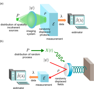
Figure 1: (a) A schematic of an incoherent imaging system, where the quantum state $\rho$ of each image-plane photon can be modeled as a randomly displaced object, with the distribution of the incoherent sources determining the probability measure $P$ for the displacement and the point-spread function of the imaging system determining the initial state $\ket{\psi}$ of the photon. (b) A schematic of an optomechanical sensor, where the quantum state $\rho$ of the optical fields before the measurement can also be modeled as a randomly displaced object, with a probability measure $P$ governing the displacement and the initial state of the optical fields determining $\ket{\psi}$. In both cases, a measurement is modeled by a positive operator-valued measure (POVM) $\mathcal{E}$, and an estimator $\check{\beta}(\lambda)$ of a parameter of $P$ can be constructed from the measurement outcome $\lambda$.

II Models

Consider first the incoherent imaging system depicted in Fig. 1(a). The one-photon density operator $\rho$ on the image plane can be modeled as Tsang et al. (2016); Tsang (2019a)

$$\rho =\int dP\ U_{X}\ket{\psi}\bra{\psi}U_{X}^{\dagger},$$ (1)

$$U_{X} =\prod_{m=1}^{M}\exp(-ik_{m}X_{m}),$$ (2)

where $M$ is the dimension of the object and image planes, $\ket{\psi}$, an element of the Hilbert space $\mathcal{H}=\mathcal{H}_{1}\otimes\dots\otimes\mathcal{H}_{M}$, models the diffraction-limited point-spread function of the imaging system, $k_{m}$ is a momentum operator on $\mathcal{H}_{m}$, $U_{X}$ is a unitary operator that models the photon displacement on the image plane due to a point source, and $X$ is a real classical $M$-dimensional random vector under the probability measure $P$, which models the object intensity function. Mathematically, Eq. (1) is a Bochner integral; both $dP$ and $X$ in Eq. (1) depend implicitly on $x\in S$ in terms of a probability space $(S,\Sigma,P)$ Holevo (2011).

The imaging problem can be framed as a quantum detection or estimation problem Tsang (2019a); Helstrom (1976), where $P$ belongs to a family of probability measures $\{P_{\theta}:\theta\in\Theta\}$ parametrized by a parameter $\theta$ in some parameter space $\Theta$ and a parameter of interest $\beta(\theta)$ is to be estimated via measurements of the optical fields. Studies in the area of quantum-inspired superresolution have shown that spatial-mode demultiplexing (SPADE) can offer a far superior performance over direct imaging and achieve the quantum limits in the resolution of two point sources Tsang et al. (2016); Lu et al. (2018), object-size estimation Tsang (2017); Dutton et al. (2019), and moment estimation Tsang (2017, 2018, 2019b); Zhou and Jiang (2019); Tsang (2019c, 2021, 2022). For the uninitiated, Appendices A and B offer a brief review of these results.

The incoherent imaging model turns out to be mathematically similar to a noise spectroscopy model also proposed by my group in Refs. Tsang and Nair (2012); Ng et al. (2016). The main difference is in the dimension $M$: imaging problems usually assume that $M$ is one or two, whereas Refs. Tsang and Nair (2012); Ng et al. (2016) assume that it is infinite. In the noise spectroscopy problem, $\rho$ is the state of a quantum dynamical system coupled to quantum fields, $\ket{\psi}$ is an element of an infinite-dimensional Hilbert space $\mathcal{H}$ that models the input state of the total system, $X(t)$ is a real classical random process with respect to a time variable $t$ that generalizes the $m$ in Eq. (2), and the unitary is

$$U_{X} =\mathcal{T}\exp[-i\int_{0}^{T}dtk(t)X(t)],$$ (3)

where $\mathcal{T}$ denotes time ordering, $T$ is the total observation time, and $k(t)$ is a Hermitian operator on $\mathcal{H}$ in an interaction picture Tsang (2013). $\ket{\psi}$ and $k(t)$ are assumed to be independent of $X$. Any sequential measurements concurrent with the displacement can be modeled as a final measurement via the principle of deferred measurement Tsang et al. (2011); Nielsen and Chuang (2011). Examples include an optical field under a random displacement or phase modulation, an optomechanical system under a stochastic force Aspelmeyer et al. (2014); Nimmrichter et al. (2014), a gravitational-wave detector under a stochastic background Christensen (2019), a spin ensemble under a stochastic magnetic field Budker and Romalis (2007), and a microwave cavity driven by dark-matter axions Backes et al. (2021). Figure 1(b) depicts an optomechanical system as an example.

References Tsang and Nair (2012); Ng et al. (2016) assume that $X(t)$ is a stationary zero-mean Gaussian random process, and its power spectral density $S_{X}(\omega|\theta)$ depends on the unknown parameter $\theta$. Reference Tsang and Nair (2012) assumes that $\Theta$ is binary with $S_{X}(\omega)=0$ for one of the hypotheses, such that the problem of interest is the detection of a random displacement, while Ref. Ng et al. (2016) assumes that $\Theta$ is a multidimensional Euclidean space, such that the problem is spectrum-parameter estimation. In other words, Refs. Tsang and Nair (2012); Ng et al. (2016) assume parametric models for the probability measure $P$, in the same way parametric models for $P$ are assumed for incoherent imaging.

III Spectrum-parameter estimation

The power spectral density, being a second-order statistic, is analogous to the second-order object moments in the context of imaging. Since SPADE can enhance the estimation of second-order moments Tsang (2017, 2018, 2019b); Zhou and Jiang (2019); Tsang (2019c, 2021, 2022), it is natural to ask if a similar enhancement can be found for noise spectroscopy. The answer is yes—Ref. Ng et al. (2016) considers an optical field under weak and random phase modulation and finds that spectral photon counting, a discrete-variable measurement analogous to SPADE, can be far superior to homodyne detection, a continuous-variable measurement analogous to direct imaging, when the input state $\ket{\psi}$ is a coherent state. Spectral photon counting is quantum-optimal and enjoys significant superiority over homodyne detection in the regime of low signal-to-noise ratios, just as SPADE is quantum-optimal and superior in the regime of subdiffraction object sizes for imaging.

In the following, I adopt a level of mathematical rigor typical of the physics and engineering literature Gardiner and Zoller (2000); Shapiro (2009) to arrive at results quickly, following Refs. Tsang and Nair (2012); Ng et al. (2016). To derive a quantum limit to noise spectroscopy, Ref. Ng et al. (2016) makes the following assumptions:

1. $X(t)$ is a zero-mean Gaussian process.

2. The processes $X(t)$ and

   $$\Delta k(t)\equiv k(t)-\bra{\psi}k(t)\ket{\psi}$$ (4)

   are stationary in the wide sense Van Trees (2001); Shumway and Stoffer (2017); Gardiner and Zoller (2000), such that

   $$C_{X}(\tau|\theta) \equiv\operatorname{\mathbb{E}}_{\theta}[X(t)X(t+\tau)],$$ (5)

   $$C_{k}(\tau) \equiv\bra{\psi}\Delta k(t)\circ\Delta k(t+\tau)\ket{\psi}$$ (6)

   are independent of $t$.

   ($\operatorname{\mathbb{E}}_{\theta}$ denotes the expectation with respect to $P_{\theta}$ and $A\circ B\equiv(AB+BA)/2$ denotes the Jordan product.)

3. The observation time $T$ is long enough to justify certain approximations regarding stationary processes Van Trees (2001); Shumway and Stoffer (2017).

Such assumptions are common in statistics Van Trees (2001); Shumway and Stoffer (2017) and have the virtue of giving simple closed-form results for the infinite-dimensional model. Assuming also that $\theta$ is a real scalar for simplicity, a quantum limit to the Fisher information $J$ for any measurement is Ng et al. (2016)

$$J \leq K\leq\tilde{K}\to T\int_{-\infty}^{\infty}\frac{d\omega}{2\pi}\frac{(\partial\ln S_{X})^{2}}{2+1/(S_{k}S_{X})},$$ (7)

$$S_{X}(\omega|\theta) \equiv\int_{-\infty}^{\infty}d\tau C_{X}(\tau|\theta)\exp(i\omega\tau),$$ (8)

$$S_{k}(\omega) \equiv\int_{-\infty}^{\infty}d\tau C_{k}(\tau)\exp(i\omega\tau),$$ (9)

where $K$ is the Helstrom information in terms of $\rho$ as a function of $\theta$ Helstrom (1976); Hayashi (2017), $\tilde{K}$ is a bound derived in Ref. Ng et al. (2016) using the extended convexity of $K$ Alipour and Rezakhani (2015), $\partial\equiv\partialderivative*{\theta}$, and $\to$ denotes the long-time limit. These information quantities determine the fundamental limits to the estimation of a parameter $\theta$ of the power spectral density $S_{X}(\omega|\theta)$ of the “noise” $X(t)$ in noise spectroscopy. For the uninitiated, Appendices A and C give a brief review of the basic concepts in quantum estimation theory.

Note that Eq. (7) is applicable to scenarios where the probe is initially entangled with an ancilla, as $\ket{\psi}$ can model the initial state of the probe plus the ancilla in a larger Hilbert space and $U_{X}$ can be an operator on the probe subspace only.

At the time of Ref. Ng et al. (2016), we were unable to find a quantum-optimal measurement when the input state is not a coherent state, but the correspondence with incoherent imaging offers a new insight. We know that SPADE can remain superior and optimal as long as its basis is adapted to $\ket{\psi}$ Tsang et al. (2016); Řeháček et al. (2017); Tsang (2018, 2021); Lu et al. (2018). This fact suggests that a discrete-variable measurement is still optimal for noise spectroscopy with a nonclassical state, as long as the measurement basis is adapted to the input state $\ket{\psi}$. If $\ket{\psi}$ is a squeezed state, it still has a Gaussian wavefunction and is analogous to a Gaussian point-spread function in imaging. The imaging correspondence then suggests that an optimal basis adapted to $\ket{\psi}$ is simply a squeezed version of an optimal basis adapted to the vacuum. A measurement in that basis can be implemented by unsqueezing the output field, analogous to an image magnification, before spectral photon counting.

I now show the optimality of the unsqueezing and spectral photon counting (USPC) method in detail. Let

$$k(t) =A^{\dagger}(t)A(t), \quantity[A(t),A^{\dagger}(t^{\prime})] =\delta(t-t^{\prime}),$$ (10)

where $A(t)$ is the annihilation operator for the slowly varying envelope of an optical field with carrier frequency $\Omega$ Gardiner and Zoller (2000); Shapiro (2009) and $k(t)$ is the photon-flux operator. $X$ is then a phase modulation on the optical field. Since $k(t)$ commutes with itself at different times, the time ordering in Eq. (3) is redundant. Assume also

$$\ket{\psi} =D(\alpha)V\ket{\textrm{vac}},$$ (11)

where $\ket{\textrm{vac}}$ is the vacuum state, $V$ is a unitary operator that models the squeezing, and $D(\alpha)$ is the displacement operator that gives a constant mean field $\bra{\psi}A(t)\ket{\psi}=\alpha$. $|\alpha|^{2}$ is the mean photon flux. With a high $|\alpha|$ and weak phase modulation, $D^{\dagger}k(t)D$ can be linearized as an intensity quadrature operator

$$D^{\dagger}k(t)D \approx|\alpha|^{2}+\kappa(t), \kappa(t) \equiv\alpha A^{\dagger}(t)+\alpha^{*}A(t),$$ (12)

and $D^{\dagger}U_{X}D$ becomes a displacement operator. This linearization turns the phase modulation into a displacement. The initial squeezing $V$ should squeeze the orthogonal phase quadrature

$$\eta(t) \equiv\frac{1}{2i|\alpha|^{2}}\quantity[\alpha A^{\dagger}(t)-\alpha^{*}A(t)]$$ (13)

and antisqueeze the intensity quadrature, such that

$$V^{\dagger}\eta V =h*\eta, V^{\dagger}\kappa V =g*\kappa,$$ (14)

where $h*\eta\equiv\int_{-\infty}^{\infty}dt^{\prime}h(t-t^{\prime})\eta(t^{\prime})$ denotes the convolution and the real Green functions $h(t)$ and $g(t)$ model the squeezing and the antisqueezing, respectively Gardiner and Zoller (2000). Their Fourier transforms are related by

$$|\tilde{h}(\omega)\tilde{g}(\omega)| =1,$$ (15)

where

$$\tilde{g}(\omega) \equiv\int_{-\infty}^{\infty}dtg(t)\exp(i\omega t),$$ (16)

and $\tilde{h}(\omega)$ is defined similarly.

After $U_{X}$, suppose that the mean field is nulled by $D^{\dagger}(\alpha)$ and then the squeezing is undone by a unitary $W$, which is the same as $V$ except that a negative sign is introduced to the parametric-amplifier Hamiltonian. In other words, the experimental setup for the unsqueezing can be the same as that for $V$, except that the phase of the pump beam should be shifted by $\pi$ if the parametric amplifier is implemented by three-wave mixing. The effect of $W$ on the quadratures can be modeled as

$$W^{\dagger}\eta W =g*\eta, W^{\dagger}\kappa W =h*\kappa.$$ (17)

Note that $W$ is not $V^{\dagger}$, as the Green functions would become anticausal and thus unphysical if $W$ were $V^{\dagger}$. Conditioned on $X$, the output state

$$\ket{\psi^{\prime}}=WD^{\dagger}U_{X}DV\ket{\textrm{vac}}$$ (18)

is a coherent state with mean field

$$\alpha^{\prime}(t) \equiv\bra{\psi^{\prime}}A(t)\ket{\psi^{\prime}}=-i\alpha g*X,$$ (19)

where the displacement in the phase quadrature is amplified by the unsqueezing. This model is also applicable to the dark port of a Michelson interferometer Caves (1981), where the squeezing $V$ and the unsqueezing $W$ should be applied to the input and output of the dark port, respectively, the displacements $D$ and $D^{\dagger}$ are naturally implemented by a strong beam at the other input port and the beam splitter in the interferometer, and $X$ is proportional to the relative phase between the two arms, as depicted by Fig. 2. Any radiation-pressure-induced noise is assumed to be negligible or eliminated Kimble et al. (2001); Tsang and Caves (2010).

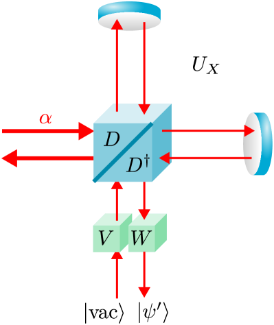
Figure 2: A Michelson implementation of the model given by Eqs. (11)–(19).

To facilitate the analysis of the subsequent step of spectral photon counting, I discretize frequency by assuming that $X(t)$ is given by the Fourier series

$$X(t) =\frac{1}{\sqrt{T}}\sum_{m=-\infty}^{\infty}\tilde{X}_{m}\exp(-i\omega_{m}t),\quad\omega_{m}\equiv\frac{2\pi m}{T},$$ (20)

$$\tilde{X}_{m} \equiv\frac{1}{\sqrt{T}}\int_{0}^{T}dtX(t)\exp(i\omega_{m}t).$$ (21)

Then the mean field of the output coherent state given by Eq. (19) can be expressed as

$$\alpha^{\prime}(t) =-\frac{i\alpha}{\sqrt{T}}\sum_{m=-\infty}^{\infty}\tilde{g}(\omega_{m})\tilde{X}_{m}\exp(-i\omega_{m}t).$$ (22)

Suppose that a spectrometer disperses the output field in terms of frequency modes defined by the annihilation operators

$$a_{m} \equiv\frac{1}{\sqrt{T}}\int_{0}^{T}dtA(t)\exp(i\omega_{m}t), m \in\mathbb{Z},$$ (23)

where $\omega_{m}$ is a sideband frequency relative to the carrier $\Omega$ Shapiro (1998). Each frequency mode is then in a coherent state with a displacement given by

$$\tilde{\alpha}_{m}\equiv\bra{\psi^{\prime}}a_{m}\ket{\psi^{\prime}}=\alpha\tilde{g}(\omega_{m})\tilde{X}_{m}.$$ (24)

Since $X(t)$ is real, $\tilde{X}_{-m}=\tilde{X}_{m}^{*}$. Assume that $\{\tilde{X}_{m}:m>0\}$ are independent zero-mean complex Gaussian random variables, each with variance

$$\operatorname{\mathbb{E}}_{\theta}(|\tilde{X}_{m}|^{2}) =S_{X}(\omega_{m}|\theta).$$ (25)

Assume also that $\tilde{X}_{0}$ is a zero-mean real Gaussian random variable that is independent of the rest. These assumptions allow the Fourier series given by Eq. (20) to approach any real stationary zero-mean Gaussian process in the long-time limit Shumway and Stoffer (2017). By summing the photon counts at each pair of sideband frequencies $-\omega_{m}$ and $\omega_{m}$, one obtains a set of photon counts that follow the Bose-Einstein distribution

$$f_{\theta}(n) =\prod_{m>0}\frac{1}{1+\bar{N}_{m}}\quantity(\frac{\bar{N}_{m}}{1+\bar{N}_{m}})^{n_{m}},$$ (26)

$$\bar{N}_{m}(\theta) =2\operatorname{\mathbb{E}}_{\theta}(|\tilde{\alpha}_{m}|^{2})=2|\alpha\tilde{g}(\omega_{m})|^{2}S_{X}(\omega_{m}|\theta).$$ (27)

The $m=0$ mode has a more complicated photon-count distribution that need not be considered, as there is a continuum of modes in the long-time limit and the information provided by one mode should be negligible. The Fisher information for USPC is hence

$$J_{\textrm{USPC}} \equiv\sum_{n}f_{\theta}(n)\quantity[\partial\ln f_{\theta}(n)]^{2}$$ (28)

$$=\sum_{m>0}\frac{(\partial\ln\bar{N}_{m})^{2}}{1+1/\bar{N}_{m}}$$ (29)

$$\to T\int_{-\infty}^{\infty}\frac{d\omega}{2\pi}\frac{(\partial\ln S_{X})^{2}}{2+1/(|\alpha\tilde{g}|^{2}S_{X})},$$ (30)

where the long-time limit gives $\sum_{m>0}\to T\int_{0}^{\infty}d\omega/(2\pi)$ and the integral $\int_{0}^{\infty}d\omega$ for an even integrand is rewritten as the double-sided integral $\int_{-\infty}^{\infty}d\omega/2$ for easier comparison with Eq. (7).

To compare this result with the quantum bound, note that the power spectral density of $\Delta k(t)$ with respect to $\ket{\psi}=DV\ket{\textrm{vac}}$ is the same as that of $\Delta k^{\prime}(t)$ with respect to $\ket{\textrm{vac}}$, where $k^{\prime}(t)\equiv V^{\dagger}D^{\dagger}k(t)DV$, and the antisqueezing of the intensity quadrature by $V$ leads to

$$S_{k}(\omega) =|\alpha\tilde{g}(\omega)|^{2}.$$ (31)

With this $S_{k}(\omega)$, the USPC information given by Eq. (30) matches the quantum bound $\tilde{K}$ given by Eq. (7) and is hence quantum-optimal.

For comparison, the Fisher information for homodyne detection of the phase quadrature $U_{X}^{\dagger}\eta U_{X}=\eta+X$ is Ng et al. (2016); Whittle (1953)

$$J_{\textrm{hom}} \to T\int_{-\infty}^{\infty}\frac{d\omega}{2\pi}\frac{(\partial\ln S_{X})^{2}}{2+4S_{\eta}/S_{X}+2(S_{\eta}/S_{X})^{2}},$$ (32)

where $\eta$ is assumed to be a stationary zero-mean Gaussian process with power spectral density $S_{\eta}$. For the squeezed $\ket{\psi}$,

$$S_{\eta}(\omega)=\frac{1}{4S_{k}(\omega)},$$ (33)

and $S_{\eta}S_{k}\geq 1/4$ in general Gardiner and Zoller (2000). Compared with the optimal information given by Eqs. (7) and (30), the homodyne information with a quantum-limited $S_{\eta}$ has an extra factor $2(S_{\eta}/S_{X})^{2}$ in the denominator, which is significant when the spectral signal-to-noise ratio (SNR) $S_{X}/S_{\eta}$ is low. To see their difference more clearly, assume

$$\frac{S_{X}}{S_{\eta}}=4S_{k}S_{X}\ll 1$$ (34)

and perform Taylor approximations of Eqs. (7), (30), and (32), which give

$$J_{\textrm{USPC}} \approx\tilde{K}\approx T\int_{-\infty}^{\infty}\frac{d\omega}{2\pi}S_{k}S_{X}(\partial\ln S_{X})^{2},$$ (35)

$$J_{\textrm{hom}} \approx 8T\int_{-\infty}^{\infty}\frac{d\omega}{2\pi}(S_{k}S_{X})^{2}(\partial\ln S_{X})^{2}.$$ (36)

$J_{\textrm{hom}}$ is much lower because of an extra factor of $8S_{k}S_{X}$ in the integrand.

For a simple example, suppose that $S_{X}(\omega|\theta)=\theta^{2}R(\omega)$, where $\theta$ is the magnitude of the displacement and $R(\omega)$ is a known spectrum. In other words, the shape of the noise spectrum is assumed to be known, and one is simply interested in estimating the height of $\sqrt{S_{X}(\omega|\theta)}$. Then

$$J_{\textrm{USPC}} \approx\tilde{K}\to T\int_{-\infty}^{\infty}\frac{d\omega}{2\pi}\frac{4}{2\theta^{2}+1/(S_{k}R)},$$ (37)

$$J_{\textrm{hom}} \to T\int_{-\infty}^{\infty}\frac{d\omega}{2\pi}\frac{4}{2\theta^{2}+1/(S_{k}R)+1/[8(\theta S_{k}R)^{2}]}.$$ (38)

As $\theta\to 0$, $J_{\textrm{hom}}$ scales quadratically with $\theta$ and vanishes, while $J_{\textrm{USPC}}$ tends to a positive constant. These behaviors are analogous to the phenomenon of Rayleigh’s curse for direct imaging and the superiority of SPADE in two-point resolution and object-size estimation Tsang et al. (2016); Tsang (2017); Dutton et al. (2019).

To be even more concrete, suppose that both $S_{k}(\omega)=|\alpha\tilde{g}(\omega)|^{2}$ and $R(\omega)$ are flat within the band $|\omega|\leq 2\pi B$ and $R(\omega)=0$ otherwise. Furthermore, assume an $R(0)$ so that $\theta^{2}$ is the spectral SNR. In other words, assume

$$S_{k}(\omega) =S_{k}(0)\textrm{ if }|\omega|\leq 2\pi B,$$ (39)

$$R(\omega) =\begin{cases}S_{\eta}(0)=1/[4S_{k}(0)],&|\omega|\leq 2\pi B,\\ 0,&\textrm{otherwise},\end{cases}$$ (40)

$$\theta^{2} =\frac{S_{X}(0|\theta)}{S_{\eta}(0)}=4S_{k}(0)S_{X}(0|\theta).$$ (41)

Then

$$J_{\textrm{USPC}} \to\frac{4BT}{\theta^{2}+2}, J_{\textrm{hom}} \to\frac{4BT}{\theta^{2}+2+1/\theta^{2}},$$ (42)

which are plotted in log-log scale in Fig. 3. Notice the difference in the scalings for $\theta\ll 1$ and the substantial widening gap.

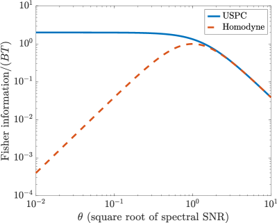
Figure 3: A comparison of USPC and homodyne detection in terms of their Fisher information given by Eqs. (42) as a function of $\theta$ in log-log scale. The Fisher information has been normalized with respect to the time-bandwidth product $BT$. $\theta$ has been normalized so that $\theta^{2}$ is the ratio of the displacement spectrum $S_{X}$ to the quantum-limited phase-quadrature spectrum $S_{\eta}=1/(4S_{k})$. Both axes are dimensionless.

In practice, the unknown parameter of the noise spectrum is, of course, often multidimensional or even the function $S_{X}$ itself with no simple parametric model. The results on multiparameter or semiparametric estimation in imaging offer encouragement that the superiority of USPC should still persist for those more complicated problems.

IV Stochastic-displacement detection

Consider now the detection problem studied in Ref. Tsang and Nair (2012). Let $\theta\in\Theta=\{0,1\}$, $P_{0}$ be the measure that gives the deterministic $X=0$ when the displacement is absent, $P_{1}$ be the measure for $X$ when the displacement is present, and $\rho_{\theta}$ be the quantum state as a function of $\theta$. Since $\rho_{0}=\ket{\psi}\bra{\psi}$ is pure in this problem, the Uhlmann fidelity is given by

$$F \equiv\tr\sqrt{\sqrt{\rho_{0}}\rho_{1}\sqrt{\rho_{0}}}=\sqrt{\bra{\psi}\rho_{1}\ket{\psi}},$$ (43)

while the quantum Chernoff exponent $\zeta$ Audenaert et al. (2008) is given by

$$\xi \leq\zeta\equiv-\ln\inf_{0\leq s\leq 1}\tr\quantity(\rho_{0}^{1-s}\rho_{1}^{s})=-2\ln F,$$ (44)

where $\xi$ is the classical Chernoff exponent for any measurement. $F$ and $\zeta$ can be used to set a variety of lower and upper bounds on the error probabilities under the Bayesian or Neyman-Pearson criterion; see Appendix D for a quick summary of the Bayesian theory.

Assuming (A1)–(A3) for $P_{1}$ and $\ket{\psi}$ and also

1. $\ket{\psi}$ is a Gaussian state,

2. $k(t)$ is a linear function of bosonic creation and annihilation operators, such that $U_{X}$ is a displacement operator,

we found that the quantum exponent is Tsang and Nair (2012)

$$\zeta \to\frac{T}{2}\int_{-\infty}^{\infty}\frac{d\omega}{2\pi}\ln\quantity(1+2S_{k}S_{X}).$$ (45)

We also considered in Ref. Tsang and Nair (2012) the performances of the Kennedy receiver and the homodyne detection for the optical model, but we were unable to find the exact optimal measurement at the time. Here I solve the open problem by showing that USPC is also optimal for the detection problem, in analogy with the optimality of SPADE for the binary-source detection problem Lu et al. (2018). Assuming again weak phase modulation, the USPC distribution given by Eqs. (26) and (27), and

$$S_{X}(\omega|0) =0, f_{0}(n) =\delta_{n0}, S_{X}(\omega|1) =S_{X}(\omega),$$ (46)

the Chernoff exponent is

$$\xi_{\textrm{USPC}} \equiv-\ln\inf_{0\leq s\leq 1}\sum_{n}\quantity[f_{0}(n)]^{1-s}\quantity[f_{1}(n)]^{s}$$ (47)

$$=\sum_{m>0}\ln\quantity[1+\bar{N}_{m}(1)]$$ (48)

$$\to\frac{T}{2}\int_{-\infty}^{\infty}\frac{d\omega}{2\pi}\ln\quantity(1+2|\alpha\tilde{g}|^{2}S_{X}).$$ (49)

With the $S_{k}$ given by Eq. (31), $\xi_{\textrm{USPC}}$ matches the quantum limit $\zeta$ given by Eq. (45).

For comparison, consider the classical Chernoff exponent for homodyne detection given by Tsang and Nair (2012); Shumway and Stoffer (2017)

$$\xi_{\textrm{hom}} \to\sup_{0\leq s\leq 1}\frac{T}{2}\int_{-\infty}^{\infty}\frac{d\omega}{2\pi}\ln\quantity[\frac{1+(1-s)S_{X}/S_{\eta}}{(1+S_{X}/S_{\eta})^{1-s}}].$$ (50)

The imaging correspondence suggests that there should be a significant gap between $\zeta$ and $\xi_{\textrm{hom}}$, although we did not realize it at the time of Ref. Tsang and Nair (2012). To demonstrate the gap now, assume again a low spectral SNR as per Eq. (34) and perform Taylor approximations of Eqs. (45), (49), and (50), which give

$$\xi_{\textrm{USPC}} \approx\zeta\approx T\int_{-\infty}^{\infty}\frac{d\omega}{2\pi}S_{k}S_{X},$$ (51)

$$\xi_{\textrm{hom}} \approx\sup_{s}\frac{s(1-s)T}{4}\int_{-\infty}^{\infty}\frac{d\omega}{2\pi}\quantity(\frac{S_{X}}{S_{\eta}})^{2}$$ (52)

$$=T\int_{-\infty}^{\infty}\frac{d\omega}{2\pi}\quantity(S_{k}S_{X})^{2}.$$ (53)

The optimal exponent is linear with respect to $S_{X}$, whereas the homodyne exponent is only quadratic. These scalings are analogous to the scalings of the optimal exponent and the direct-imaging exponent with respect to the source separation in the binary-source detection problem Lu et al. (2018).

For a more concrete example, assume the flat spectra given by Eqs. (39) and (40) and define

$$S_{X}(\omega) =\phi^{2}R(\omega),$$ (54)

so that the spectral SNR is now $\phi^{2}$, and $\phi$ plays the same role as $\theta$ in Fig. 3. Figure 4 plots the resulting Chernoff exponents given by Eqs. (49) and (50) against $\phi$ in log-log scale.

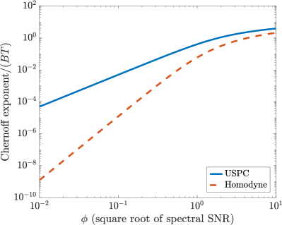
Figure 4: A comparison of USPC and homodyne detection in terms of their Chernoff exponents given by Eqs. (49) and (50), assuming the flat spectra given by Eqs. (39) and (40). The horizontal axis $\phi$ is the square root of the spectral SNR defined by Eq. (54). The Chernoff exponent has been normalized with respect to the time-bandwidth product $BT$. The plot is in log-log scale and both axes are dimensionless.

It is possible to study the error probabilities of the detection problem more precisely under the Neyman-Pearson criterion Tsang and Nair (2012); Hayashi (2017); Huang and Lupo (2021); Zanforlin et al. (2022), although the insights offered by such calculations should not deviate much from the ones reported here.

V Discussion

Since homodyne detection is the current standard measurement method in gravitational-wave detection Danilishin et al. (2019), the superior scalings of the USPC information quantities indicated by Eqs. (35), (36), (51), and (53) are important discoveries. They suggest that USPC can substantially enhance the detection and spectroscopy of stochastic gravitational-wave backgrounds when the spectral SNR is low, in the same way SPADE can enhance incoherent imaging. Considering that squeezed light is now being used in gravitational-wave detectors M. Tse et al. (2019), the unsqueezing step proposed here is important, as it optimizes the measurement for squeezed light beyond the coherent-state case considered in Refs. Tsang and Nair (2012); Ng et al. (2016) and allows the full potential of quantum-enhanced interferometry to be realized for noise spectroscopy.

A potential practical issue with the proposal is its assumption of quantum-limited squeezing and unsqueezing in both quadratures. Optical squeezers in current technology often introduce excess noise in the antisqueezed quadrature, which has little impact on the homodyne detection of the squeezed quadrature but may add significant noise to the photon counting step here. With two squeezers in the proposed setup, the issue of excess noise is even worse. In view of the amazing achievements of the experimentalists in LIGO and squeezing, however, one should never underestimate their skills, and the superiority of USPC should motivate the current and future generations to reach even greater heights in squeezing technology in order to achieve the promised improvement.

The correspondence between the incoherent imaging model and the random displacement model is used implicitly in Section 6 of Ref. Tsang (2017) and briefly mentioned in Ref. Tsang (2019b) but not elaborated there. References Gefen et al. (2019); Mouradian et al. (2021) point out the correspondence between incoherent imaging and noise spectroscopy more explicitly, although they assume a low dimension for the Hilbert space and somewhat different parametric models. A more recent outstanding work by Górecki, Riccardi, and Maccone Górecki et al. (2022) also notices the correspondence and also uses the convexity of the Helstrom information to derive a quantum bound for a random displacement model with one optical mode. They discovered independently that unsqueezing before photon counting is optimal for a squeezed input state and superior to homodyne detection. Another outstanding relevant work is Ref. Shi and Zhuang (2022) by Shi and Zhuang, who also discovered independently the optimality and superiority of unsqueezing and photon counting for a somewhat different random displacement model, which can be obtained by applying a rotating-wave approximation to the unitary given by Eq. (3) and imposing a thermal channel. References Gefen et al. (2019); Mouradian et al. (2021); Górecki et al. (2022); Shi and Zhuang (2022) all do not consider the detection problem and are not aware of the prior Refs. Tsang and Nair (2012); Ng et al. (2016).

As there exist many other results in quantum-inspired superresolution that have not yet been translated to noise spectroscopy, and vice versa, the correspondence between the two models should have a lot more to give.

Appendix A Quantum estimation theory

Let $\{\rho_{\theta}:\theta\in\Theta\}$ be a family of density operators. Given a parameter $\theta$ and after a measurement modeled by a positive operator-valued measure (POVM) $\mathcal{E}$, the probability measure $Q_{\theta}$ for the measurement outcome $\lambda$ being in a set $A$ is given by Holevo (2011)

$$Q_{\theta}(A) =\tr\mathcal{E}(A)\rho_{\theta},$$ (55)

where $\tr$ is the operator trace. Let the parameter of interest be a real scalar $\beta(\theta)$ and an estimator be $\check{\beta}(\lambda)$. The mean-square error is defined as

$$\operatorname{MSE}(\theta) \equiv\operatorname{\mathbb{E}}_{\theta}\left\{\left[\check{\beta}-\beta(\theta)\right]^{2}\right\}$$ (56)

$$=\int dQ_{\theta}(\lambda)\left[\check{\beta}(\lambda)-\beta(\theta)\right]^{2},$$ (57)

where $\operatorname{\mathbb{E}}_{\theta}$ denotes the expectation given $\theta$. Let $\theta$ be a real scalar and suppose that each $Q_{\theta}$ possesses a probability density $f_{\theta}(\lambda)$ with respect to a $\theta$-independent reference measure $\nu$. Assuming the local unbiased condition for the estimator given by

$$\operatorname{\mathbb{E}}_{\theta}\left(\check{\beta}\right) =\beta(\theta),$$ (58)

$$\int d\nu(\lambda)\check{\beta}(\lambda)\partial f_{\theta}(\lambda) =\operatorname{\mathbb{E}}_{\theta}\left(\check{\beta}\partial\ln f_{\theta}\right)=\partial\beta(\theta),$$ (59)

$$\partial \equiv\partialderivative{\theta},$$ (60)

the classical Cramér-Rao bound is

$$\operatorname{MSE}(\theta) \geq\frac{[\partial\beta(\theta)]^{2}}{J(\theta)}, J(\theta) \equiv\operatorname{\mathbb{E}}_{\theta}\left[\left(\partial\ln f_{\theta}\right)^{2}\right],$$ (61)

where $J(\theta)$ is called the Fisher information. The bound is also achievable with the maximum-likelihood estimator in an asymptotic sense and can be generalized for more relaxed conditions Van Trees (2001).

A quantum bound on $J$ for any POVM $\mathcal{E}$ is Hayashi (2017)

$$J(\theta) \leq K(\theta)\equiv\tr\rho_{\theta}L_{\theta}^{2},$$ (62)

where $K(\theta)$ is the Helstrom information Helstrom (1976), $L_{\theta}$ is a solution to

$$\partial\rho_{\theta} =\rho_{\theta}\circ L_{\theta},$$ (63)

and $\circ$ denotes the Jordan product of two operators defined as

$$A\circ B \equiv\frac{1}{2}\left(AB+BA\right).$$ (64)

Generalization of these results for a multidimensional parameter can be done by considering the matrix versions of the information quantities Hayashi (2017) or adopting the parametric-submodel approach Tsang et al. (2020); Gross and Caves (2020); Tsang (2021).

Appendix B Quantum-inspired superresolution

Consider the incoherent imaging model given by Eqs. (1) and (2) in one dimension ($M=1$). For the estimation of the separation between two point sources, the probability measure $P_{\theta}$ as a function of the separation $\theta\in\mathbb{R}$ can be modeled as

$$P_{\theta} =\frac{1}{2}\left(\delta_{-\theta/2}+\delta_{\theta/2}\right),$$ (65)

where

$$\delta_{x}(A) \equiv\begin{cases}1,&x\in A,\\ 0,&\textrm{otherwise}\end{cases}$$ (66)

is the Dirac measure for a unit point mass at position $x$. With direct imaging, which can be modeled as a measurement of the continuous photon position, the Fisher information $J(\theta)$ is roughly constant for large $\theta$ relative to Rayleigh’s criterion, but it decreases when $\theta$ becomes sub-Rayleigh and drops to zero when $\theta=0$. To distinguish this soft penalty to the Fisher information from the more heuristic Rayleigh’s criterion, Ref. Tsang et al. (2016) calls the penalty Rayleigh’s curse.

Unlike the direct-imaging Fisher information under Rayleigh’s curse, the Helstrom information $K(\theta)$ for this problem is constant regardless of $\theta$, meaning that the ultimate information in the photons is substantially higher than the direct-imaging information for sub-Rayleigh separations. Moreover, a measurement in the discrete Hermite-Gaussian basis called SPADE has a Fisher information that coincides with the Helstrom information for all $\theta$, meaning that SPADE is an optimal measurement and can be far superior to direct imaging for sub-Rayleigh separations Tsang et al. (2016).

A similar scenario plays out when one attempts to estimate the size of an object, for which the probability density of $P_{\theta}$ can be expressed as

$$\derivative{P_{\theta}}{X} =\frac{1}{\theta}w\quantity(\frac{X}{\theta})$$ (67)

in terms of a known function $w$ Tsang (2017); Dutton et al. (2019). For this problem, Rayleigh’s curse can also be observed in the direct-imaging information, while the Helstrom information and the SPADE information approach a nonzero constant for sub-Rayleigh separations.

References Tsang (2017, 2018, 2019b); Zhou and Jiang (2019); Tsang (2019c, 2021, 2022) study the moment estimation problem, assuming that $\theta=P$, $\Theta$ is the set of all probability meaures, while the parameter of interest is

$$\beta(P) =\int dP(X)b(X),$$ (68)

such as the second moment with $b(X)=X^{2}$. As the parameter space is now infinite-dimensional, the theory becomes much more formidable. Yet, with some effort, it can still be shown that SPADE enjoys a significant superiority over direct imaging for sub-Rayleigh object sizes and is close to quantum-optimal.

Appendix C Extended convexity

As the Helstrom information $K(\theta)$ is often difficult to compute, especially if the density operators are mixed, one may have to settle for looser bounds. If the density operator can be expressed as the mixture

$$\rho_{\theta} =\int dP_{\theta}(Z)\sigma_{\theta}(Z),$$ (69)

where $\sigma_{\theta}(Z)$ is a density operator conditioned on the random element $Z$, then a useful bound on $K(\theta)$ called the extended convexity is Alipour and Rezakhani (2015); Ng et al. (2016)

$$K(\theta)\leq\tilde{K}(\theta) \equiv\int dP_{\theta}(Z)K[\sigma_{\theta}(Z)]+J[P_{\theta}],$$ (70)

where $K[\sigma_{\theta}(Z)]$ is the Helstrom information in terms of $\sigma_{\theta}(Z)$ and $J[P_{\theta}]$ is the Fisher information in terms of $P_{\theta}$.

To offer some intuition about the use of the extended-convexity bound in Ref. Ng et al. (2016), consider the model given by Eqs. (1) and (2) in one dimension ($M=1$) for simplicity. Let

$$dP_{\theta} =\frac{1}{\sqrt{2\pi v_{X}(\theta)}}\exp[-\frac{X^{2}}{2v_{X}(\theta)}]dX,$$ (71)

such that the variance $v_{X}(\theta)$ of the displacement $X$ depends on the unknown parameter. A trick to derive a good bound is to change the random variable to $Z=X/\gamma(\theta)$ in terms of a judiciously chosen function $\gamma(\theta)$, such that

$$dP_{\theta} =\frac{\gamma(\theta)}{\sqrt{2\pi v_{X}(\theta)}}\exp[-\frac{\gamma(\theta)^{2}Z^{2}}{2v_{X}(\theta)}]dZ,$$ (72)

$$\sigma_{\theta}(Z) =U_{\gamma(\theta)Z}\ket{\psi}\bra{\psi}U_{\gamma(\theta)Z}^{\dagger}.$$ (73)

These expressions lead to

$$K[\sigma_{\theta}(Z)] =4v_{k}(\partial\gamma)^{2}Z^{2},$$ (74)

$$v_{k} \equiv\bra{\psi}k^{2}\ket{\psi}-(\bra{\psi}k\ket{\psi})^{2},$$ (75)

$$\int dP_{\theta}(Z)K[\sigma_{\theta}(Z)] =4v_{k}v_{X}(\partial\ln\gamma)^{2},$$ (76)

$$J[P_{\theta}] =\frac{1}{2}\left[\partial\ln\left(\frac{v_{X}}{\gamma^{2}}\right)\right]^{2},$$ (77)

$$\tilde{K}(\theta) =4v_{k}v_{X}(\partial\ln\gamma)^{2}$$

$$\quad+\frac{1}{2}\left(\partial\ln v_{X}-2\partial\ln\gamma\right)^{2},$$ (78)

where Eq. (76) assumes that $v_{k}$ and $\gamma$ do not depend on the random variable. Picking

$$\partial\ln\gamma=\frac{\partial\ln v_{X}}{2+4v_{k}v_{X}}$$ (79)

hence leads to

$$\tilde{K}(\theta) =\frac{(\partial\ln v_{X})^{2}}{2+1/(v_{k}v_{X})},$$ (80)

which resembles Eq. (7). The derivation of Eq. (7) in Ref. Ng et al. (2016) indeed follows a similar procedure.

If $P_{\theta}$ is not Gaussian, a bound may still be obtained by using the convexity of the Helstrom information; Section 6 of Ref. Tsang (2017) uses the convexity to derive a quantum limit to object-size estimation in the context of imaging and shows that SPADE can approach the limit. The trick is to change the variable in Eq. (67) to $Z=X/\theta$, leading to

$$\rho_{\theta} =\int dZw(Z)\sigma_{\theta}(Z), \sigma_{\theta}(Z) =U_{\theta Z}\ket{\psi}\bra{\psi}U_{\theta Z}^{\dagger}.$$ (81)

As $w(Z)$ no longer depends on $\theta$, Eq. (70) gives the convexity bound

$$\tilde{K}(\theta)=\int dZw(Z)K[\sigma_{\theta}(Z)]=4v_{k}\int dZw(Z)Z^{2},$$ (82)

which is independent of $\theta$. It turns out that SPADE can achieve this bound in the limit of $\theta\to 0$ Tsang (2017). Reference Górecki et al. (2022) has obtained similar results.

Appendix D Quantum detection theory

Assume two hypotheses $\Theta=\{0,1\}$. Let $A$ be the set of measurement outcomes with which one decides on $\theta=0$ and $A^{c}$ be the set with which one decides on $\theta=1$. Then the type-I and type-II error probabilities are, respectively,

$$Q_{0}(A^{c}) =\tr\mathcal{E}(A^{c})\rho_{0}, Q_{1}(A) =\tr\mathcal{E}(A)\rho_{1}.$$ (83)

Let $\pi_{\theta}$ be the prior probability of the hypothesis $\theta$. Then the average error probability is

$$P_{e} \equiv\pi_{0}Q_{0}(A^{c})+\pi_{1}Q_{1}(A).$$ (84)

Given a measurement, the classical detection problem is to choose a set $A$ that minimizes the error probabilities. In particular, $P_{e}$ can be minimized by a likelihood-ratio test Van Trees (2001). Denote this minimum $P_{e}$ by $P_{e,\textrm{min}}$ and assume $\pi_{0}=\pi_{1}=1/2$ for simplicity. A useful lower bound on $P_{e,\textrm{min}}$ is Kailath (1967)

$$P_{e} \geq P_{e,\textrm{min}}\geq\frac{1}{2}\left(1-\sqrt{1-B^{2}}\right),$$ (85)

where

$$B \equiv\int d\nu(\lambda)\sqrt{f_{0}(\lambda)f_{1}(\lambda)}$$ (86)

is the Bhattacharyya coefficient. Another useful bound is the Chernoff bound given by Van Trees (2001)

$$P_{e,\textrm{min}} \leq\frac{1}{2}\exp(-\xi),$$ (87)

$$\xi \equiv-\ln\inf_{0\leq s\leq 1}\int d\nu(\lambda)[f_{0}(\lambda)]^{1-s}[f_{1}(\lambda)]^{s}.$$ (88)

The error exponent $-\ln P_{e,\textrm{min}}$ approaches the Chernoff exponent $\xi$ in an asymptotic sense Levy (2008).

For any POVM $\mathcal{E}$, a quantum lower bound on $B$ is Hayashi (2017)

$$B \geq F\equiv\tr\sqrt{\sqrt{\rho_{0}}\rho_{1}\sqrt{\rho_{0}}},$$ (89)

where $F$ is the Uhlmann fidelity, while a quantum upper bound on $\xi$ is Audenaert et al. (2008)

$$\xi \leq\zeta\equiv-\ln\inf_{0\leq s\leq 1}\tr\quantity(\rho_{0}^{1-s}\rho_{1}^{s}).$$ (90)

References

- Tsang et al. (2016) Mankei Tsang, Ranjith Nair, and Xiao-Ming Lu, “Quantum theory of superresolution for two incoherent optical point sources,” Physical Review X 6, 031033 (2016).
- Tsang (2019a) Mankei Tsang, “Resolving starlight: a quantum perspective,” Contemporary Physics 60, 279–298 (2019a).
- Tsang and Nair (2012) Mankei Tsang and Ranjith Nair, “Fundamental quantum limits to waveform detection,” Physical Review A 86, 042115 (2012).
- Ng et al. (2016) Shilin Ng, Shan Zheng Ang, Trevor A. Wheatley, Hidehiro Yonezawa, Akira Furusawa, Elanor H. Huntington, and Mankei Tsang, “Spectrum analysis with quantum dynamical systems,” Physical Review A 93, 042121 (2016).
- Budker and Romalis (2007) Dmitry Budker and Michael Romalis, “Optical magnetometry,” Nature Physics 3, 227–234 (2007).
- Backes et al. (2021) K. M. Backes, D. A. Palken, S. Al Kenany, B. M. Brubaker, S. B. Cahn, A. Droster, Gene C. Hilton, Sumita Ghosh, H. Jackson, S. K. Lamoreaux, A. F. Leder, K. W. Lehnert, S. M. Lewis, M. Malnou, R. H. Maruyama, N. M. Rapidis, M. Simanovskaia, Sukhman Singh, D. H. Speller, I. Urdinaran, Leila R. Vale, E. C. van Assendelft, K. van Bibber, and H. Wang, “A quantum enhanced search for dark matter axions,” Nature 590, 238–242 (2021).
- Holevo (2011) Alexander S. Holevo, Probabilistic and Statistical Aspects of Quantum Theory (Scuola Normale Superiore Pisa, Pisa, Italy, 2011).
- Helstrom (1976) Carl W. Helstrom, Quantum Detection and Estimation Theory (Academic Press, New York, 1976).
- Lu et al. (2018) Xiao-Ming Lu, Hari Krovi, Ranjith Nair, Saikat Guha, and Jeffrey H. Shapiro, “Quantum-optimal detection of one-versus-two incoherent optical sources with arbitrary separation,” npj Quantum Information 4, 64 (2018).
- Tsang (2017) Mankei Tsang, “Subdiffraction incoherent optical imaging via spatial-mode demultiplexing,” New Journal of Physics 19, 023054 (2017).
- Dutton et al. (2019) Zachary Dutton, Ronan Kerviche, Amit Ashok, and Saikat Guha, “Attaining the quantum limit of superresolution in imaging an object’s length via predetection spatial-mode sorting,” Physical Review A 99, 033847 (2019).
- Tsang (2018) Mankei Tsang, “Subdiffraction incoherent optical imaging via spatial-mode demultiplexing: Semiclassical treatment,” Physical Review A 97, 023830 (2018).
- Tsang (2019b) Mankei Tsang, “Quantum limit to subdiffraction incoherent optical imaging,” Physical Review A 99, 012305 (2019b).
- Zhou and Jiang (2019) Sisi Zhou and Liang Jiang, “Modern description of Rayleigh’s criterion,” Physical Review A 99, 013808 (2019).
- Tsang (2019c) Mankei Tsang, “Semiparametric estimation for incoherent optical imaging,” Physical Review Research 1, 033006 (2019c).
- Tsang (2021) Mankei Tsang, “Quantum limit to subdiffraction incoherent optical imaging. II. A parametric-submodel approach,” Physical Review A 104, 052411 (2021).
- Tsang (2022) Mankei Tsang, “Efficient superoscillation measurement for incoherent optical imaging,” arXiv:2010.11084 (2022).
- Tsang (2013) Mankei Tsang, “Quantum metrology with open dynamical systems,” New Journal of Physics 15, 073005 (2013).
- Tsang et al. (2011) Mankei Tsang, Howard M. Wiseman, and Carlton M. Caves, “Fundamental Quantum Limit to Waveform Estimation,” Physical Review Letters 106, 090401 (2011).
- Nielsen and Chuang (2011) Michael A. Nielsen and Isaac L. Chuang, Quantum Computation and Quantum Information (Cambridge University Press, Cambridge, 2011).
- Aspelmeyer et al. (2014) Markus Aspelmeyer, Tobias J. Kippenberg, and Florian Marquardt, “Cavity optomechanics,” Rev. Mod. Phys. 86, 1391–1452 (2014).
- Nimmrichter et al. (2014) Stefan Nimmrichter, Klaus Hornberger, and Klemens Hammerer, “Optomechanical sensing of spontaneous wave-function collapse,” Physical Review Letters 113, 020405 (2014).
- Christensen (2019) Nelson Christensen, “Stochastic gravitational wave backgrounds,” Reports on Progress in Physics 82, 016903 (2019).
- Gardiner and Zoller (2000) Crispin W. Gardiner and Peter Zoller, Quantum Noise, 2nd ed. (Springer-Verlag, Berlin, 2000).
- Shapiro (2009) Jeffrey H. Shapiro, “The quantum theory of optical communications,” IEEE Journal of Selected Topics in Quantum Electronics 15, 1547–1569 (2009).
- Van Trees (2001) Harry L. Van Trees, Detection, Estimation, and Modulation Theory, Part I. (John Wiley & Sons, New York, 2001).
- Shumway and Stoffer (2017) Robert H. Shumway and David S. Stoffer, Time Series Analysis and Its Applications (Springer, Cham, Switzerland, 2017).
- Hayashi (2017) Masahito Hayashi, Quantum Information Theory: Mathematical Foundation, 2nd ed. (Springer, Berlin, 2017).
- Alipour and Rezakhani (2015) S. Alipour and A. T. Rezakhani, “Extended convexity of quantum Fisher information in quantum metrology,” Physical Review A 91, 042104 (2015).
- Řeháček et al. (2017) J. Řeháček, M. Paúr, B. Stoklasa, Z. Hradil, and L. L. Sánchez-Soto, “Optimal measurements for resolution beyond the Rayleigh limit,” Optics Letters 42, 231–234 (2017).
- Caves (1981) Carlton M. Caves, “Quantum-mechanical noise in an interferometer,” Physical Review D 23, 1693–1708 (1981).
- Kimble et al. (2001) H. J. Kimble, Yuri Levin, Andrey B. Matsko, Kip S. Thorne, and Sergey P. Vyatchanin, “Conversion of conventional gravitational-wave interferometers into quantum nondemolition interferometers by modifying their input and/or output optics,” Physical Review D 65, 022002 (2001).
- Tsang and Caves (2010) Mankei Tsang and Carlton M. Caves, “Coherent Quantum-Noise Cancellation for Optomechanical Sensors,” Physical Review Letters 105, 123601 (2010).
- Shapiro (1998) Jeffrey H. Shapiro, “Quantum measurement eigenkets for continuous-time direct detection,” Quantum and Semiclassical Optics: Journal of the European Optical Society Part B 10, 567 (1998).
- Whittle (1953) P. Whittle, “The analysis of multiple stationary time series,” Journal of the Royal Statistical Society. Series B (Methodological) 15, pp. 125–139 (1953).
- Audenaert et al. (2008) K.M.R. Audenaert, M. Nussbaum, A. Szkoła, and F. Verstraete, “Asymptotic error rates in quantum hypothesis testing,” Communications in Mathematical Physics 279, 251–283 (2008).
- Huang and Lupo (2021) Zixin Huang and Cosmo Lupo, “Quantum hypothesis testing for exoplanet detection,” Physical Review Letters 127, 130502 (2021).
- Zanforlin et al. (2022) Ugo Zanforlin, Cosmo Lupo, Peter W. R. Connolly, Pieter Kok, Gerald S. Buller, and Zixin Huang, “Optical quantum super-resolution imaging and hypothesis testing,” Nature Communications 13, 5373 (2022).
- Danilishin et al. (2019) Stefan L. Danilishin, Farid Ya. Khalili, and Haixing Miao, “Advanced quantum techniques for future gravitational-wave detectors,” Living Reviews in Relativity 22, 2 (2019).
- M. Tse et al. (2019) M. Tse et al., “Quantum-Enhanced Advanced LIGO Detectors in the Era of Gravitational-Wave Astronomy,” Physical Review Letters 123, 231107 (2019).
- Gefen et al. (2019) T. Gefen, A. Rotem, and A. Retzker, “Overcoming resolution limits with quantum sensing,” Nature Communications 10, 4992 (2019).
- Mouradian et al. (2021) Sara L. Mouradian, Neil Glikin, Eli Megidish, Kai-Isaak Ellers, and Hartmut Haeffner, “Quantum sensing of intermittent stochastic signals,” Physical Review A 103, 032419 (2021).
- Górecki et al. (2022) Wojciech Górecki, Alberto Riccardi, and Lorenzo Maccone, “Quantum metrology of noisy spreading channels,” ArXiv e-prints (2022), 10.48550/arXiv.2208.09386, 2208.09386 .
- Shi and Zhuang (2022) Haowei Shi and Quntao Zhuang, “Ultimate precision limit of noise sensing and dark matter search,” ArXiv e-prints (2022), 10.48550/arXiv.2208.13712, 2208.13712 .
- Tsang et al. (2020) Mankei Tsang, Francesco Albarelli, and Animesh Datta, “Quantum Semiparametric Estimation,” Physical Review X 10, 031023 (2020).
- Gross and Caves (2020) Jonathan Arthur Gross and Carlton M. Caves, “One from many: Estimating a function of many parameters,” Journal of Physics A: Mathematical and Theoretical 54, 014001 (2020).
- Kailath (1967) Thomas Kailath, “The divergence and Bhattacharyya distance measures in signal selection,” IEEE Transactions on Communication Technology 15, 52–60 (1967).
- Levy (2008) Bernard C. Levy, Principles of Signal Detection and Parameter Estimation (Springer, New York, 2008).