Bimanual crop manipulation for human-inspired robotic harvesting

Abstract

Most existing robotic harvesters utilize a unimanual approach; a single arm grasps the crop and detaches it, either via a detachment movement, or by cutting its stem with a specially designed gripper/cutter end-effector. However, such unimanual solutions cannot be applied for sensitive crops and cluttered environments like grapes and a vineyard where obstacles may occlude the stem and leave no space for the cutter’s placement. In such cases, the solution would require a bimanual robot in order to visually unveil the stem and manipulate the grasped crop to create cutting affordances which is similar to the practice used by humans. In this work, a dual-arm coordinated motion control methodology for reaching a stem pre-cut state is proposed. The camera equipped arm with the cutter is reaching the stem, unveiling it as much as possible, while the second arm is moving the grasped crop towards the surrounding free-space to facilitate its stem cutting. Lab experimentation on a mock-up vine setup with a plastic grape cluster evaluates the proposed methodology, involving two UR5e robotic arms and a RealSense D415 camera.

I Introduction

In the last decade, development of robotic technologies and their application in agricultural tasks are becoming a growing topic of interest [Marinoudi]. The rising of food supply demands, climate change, land degradation and arable land limitations have all pushed towards agricultural productivity growth becoming an important priority. Incorporating advanced, automated, agricultural technologies is bound to greatly benefit productivity and in turn economic development [Eberhardt], while at the same time facilitating and improving the difficult working conditions of farmers and agricultural workers [Fathallah]. In this context, an increasing amount of research work has been noticed during the last years [Fountas, Bac]. Various agricultural tasks are considered as potential applications of robotic solutions developed in literature e.g. yield estimation, phenotyping, pruning, as well as crop harvesting. Earlier solutions in crop harvesting involved the bulk concept (i.e. tree trunk/branch shaking), however the selective concept has been mostly adopted lately, since it entails considerably less danger of harming the crops. In selective harvesting, the robotic system firstly detects a specific harvest target and then harvests it.

A variety of integrated robotic solutions have been proposed towards this end [Ramin], with the majority of them utilizing one robotic manipulator (unimanual setup), responsible for monitoring the target crop via a mounted in-hand camera and harvesting it, i.e. grasping it and detaching it. In [Onishi], [Silwal] a detaching movement performed by the arm’s gripper e.g. pulling and twisting the grasped crop in order to cause the stem’s breaking and crop’s release. However, detaching movements are only applicable on rigid crops (e.g. apples) that can withstand such treatment without being damaged. Alternatively, various approaches utilize the grasped crops stem cutting and mainly involve: (a) a cutting tool embodied in the gripper that cuts the stem after the crop is grasped [sHayashi], [VanHenten]; (b) a specially designed cutter end-effector, responsible for simultaneously cutting and holding the crop by its stem [Feng], [Hayashi2]. In these works, harvesting of eggplants, cucumbers, tomatoes and strawberries is performed. Such unimanual solution may work after certain crop modification e.g. pruning or cultivation/farming methodologies specifically designed to be more ”friendly” towards automated/robotic harvesting such as the cucumber high-wire system [VanHenten] and the apple V-trellis system [Silwal]. However, in general, such unimanual solutions cannot be applied for sensitive and cluttered environments like a vineyard where poles, wires, flexible branches and leaves and even the crop itself partially occlude the stem, which can be further wrapped partially around a branch leaving no space for the cutter placement. In such cases the solution would require a bimanual robot in order to visually unveil the stem and manipulate the grasped crop to create cutting affordances. Notice that grape harvesting is performed bimanually by humans. In fact, a very common approach that humans apply during grape harvesting, is to grasp with one arm the crop, moving their head and body to be able to see the stem and manipulate the crop, if needed, in order to provide sufficient free room around the stem for the cutting tool held by their other arm (Fig. 1).

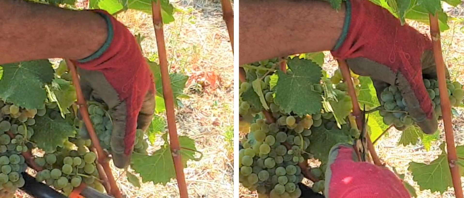
Figure 1: Bimanual human harvesting

There are few works in literature, proposing a dual-arm/bimanual solution [Zhao, Ling]. In [Zhao], a dual-arm tomato harvesting robot is designed, with two 3 degrees of freedom (DOF) SCARA manipulators (one prismatic and two revolute joints) and two different end-effectors (vacuum suction gripper and saw cutting tool). In [Ling], the same robotic solution is further developed, introducing autonomous ripe tomato detection in contrast to [Zhao] where human collaboration was required, evaluated in a simple environment with several potted tomatoes placed in rows. However, the limited manipulability of the arms due to few DOF and the very specific gripper’s design considering only rigid, spherical crops would render the above solution’s application very difficult in more challenging crops/environments, such as grapes/vineyards.

In this work, we consider a bimanual robot with one arm equipped with a crop specific gripper (grasping arm) and the other with a stem cutting tool and a camera mounted on its end-effector (camera arm). Our focus is on the core bimanual task of approaching while unveiling the stem by the camera arm, while manipulating the grasped crop with the other arm for generating cutting affordances. Reaching to grasp the crop and reaching the final cut pose to cut the stem from a precut pose are mainly unimanual operations, which can be addressed by methods already proposed in the literature, like grasp planning [Sahbani] and visual-servoing [Ringdahl].

II Problem Description

We consider a robot with two robotic arms: (a) the grasping arm of $N_{g}\in\mathbb{N}$ degrees of freedom (DOF) with $\mathbf{q}_{g}\in\mathbb{R}^{N_{g}}$ its joints vector, responsible for the stable grasping and manipulation of target crop; (b) the camera arm of $N_{c}\in\mathbb{N}$ DOF and joint vector $\mathbf{q}_{c}\in\mathbb{R}^{N_{c}}$ that monitors the whole scene via a mounted, in-hand, RGB-D camera equipped with a cutting tool. As an initial state for the robot we consider that the grasping arm has achieved grasping of the crop by its gripper and that a point-cloud of the overall scene is provided by the camera arm. We assume that an appropriate vision algorithm/methodology designed specifically for recognizing the stem is available. Notice that this assumption does not exclude the case of a stem being partially occluded or initially not recognized.

Let $\mathbf{T}_{c}\in SE(3)$ be the homogeneous transformation expressing the generalized pose of the camera’s frame $\{C\}$ (which is in our case placed at the camera arm’s tip) with respect to the world inertial frame $\{0\}$; it involves its position $\mathbf{p}_{c}(\mathbf{q}_{c})\in\mathbb{R}^{3}$ and its orientation $\mathbf{R}_{c}(\mathbf{q}_{c})\triangleq[\mathbf{x}_{c}\;\mathbf{y}_{c}\;\mathbf{z}_{c}]\in SO(3)$, that are both known via the camera arm’s kinematics. Additionally, let $\mathbf{T}_{g}\in SE(3)$ be the homogeneous transformation expressing the grasping arm’s tip/grasped crop frame $\{G\}$ with respect to $\{0\}$, involving position $\mathbf{p}_{g}(\mathbf{q}_{g})\in\mathbb{R}^{3}$ and orientation $\mathbf{R}_{g}(\mathbf{q}_{g})\triangleq[\mathbf{x}_{g}\;\mathbf{y}_{g}\;\mathbf{z}_{g}]\in SO(3)$, known via the grasping arm’s kinematics.

The core bimanual task of approaching and unveiling the stem with the camera arm and manipulating the grasped crop with the grasping arm, which is addressed in this work, is a bimanual asymmetric task where each arm’s controller has a different objective but their motion needs appropriate planning and coordination. In particular, the camera arm’s controller should operate in a clutter dynamical scene in which changes are not only induced by dynamic changes in the environment (e.g wind gusts can move the surrounding leaves) but also by the grasping arm’s manipulation of the crop. In the following two subsections each arm’s control objectives are presented.

II-A Camera arm control objectives

The camera arm is responsible for reaching a predefined region of interest (ROI) surrounding the crop and its stem and adopt a pose in this region that allows the stem to be unveiled as much as possible thus getting sufficiently close to it into a pre-cutting position. We can therefore distinguish two objectives that should be simultaneously satisfied by this controller, reaching and centering, and unveiling.

We model the ROI by a sphere and we call the associated stem, object of interest (OOI); let $\mathbf{p}_{r}\in\mathbb{R}^{3}$ be the center of ROI in the inertia frame with $r\in\mathbb{R}_{>0}$ its radius. The reaching and centering objective aims at moving the camera arm’s end-effector to any of the ROI points, while aligning the camera’s $Z$ axis with the vector pointing to the ROI center. The ROI center can be placed on a point on the stem if it is initially partially recognized or on the grape otherwise. As the camera moves closer and visual feedback provides better estimates of the point-cloud of the grape and its stem it is updated. To prevent discontinuities in the arm’s operation the center of ROI displacement is smoothed by a filter. The two objectives can be formulated as follows:

1. Reaching and centering:

   for reaching the following should hold true: $\|\mathbf{p}_{r}-\mathbf{p}_{c}\|\rightarrow\overline{r}\leq r$ for $t\rightarrow\infty$ and some scalar positive $\overline{r}$; regarding centering, the angle between $\mathbf{p}_{r}-\mathbf{p}_{c}$ and the camera’s view direction $\mathbf{z}_{c}$ defined as $\theta(\mathbf{p}_{c},\mathbf{p}_{r})\triangleq\text{cos}^{-1}\left(\frac{\mathbf{z}_{c}^{\intercal}(\mathbf{p}_{r}-\mathbf{p}_{c})}{\|\mathbf{p}_{r}-\mathbf{p}_{c}\|}\right)$ should satisfy $\theta(\mathbf{p}_{c},\mathbf{p}_{r})\rightarrow 0$ for $t\rightarrow\infty$.

2. Unveiling: maximize the visible part of the OOI, i.e. maximize the perceived number of points of the point-cloud that belong to the stem.

Notice that $\theta\rightarrow 0$ involved in the first objective maintains the ROI center at the center of the camera’s field of view, thus securing the best ROI and OOI viewpoint. Moreover, notice that $\theta$ cannot be more than $\nicefrac{{\pi}}{{2}}$, since the ROI center $\mathbf{p}_{r}$ is within the camera’s field of view, i.e. a pyramid.

Clearly, the reaching and centering objective is achieved by reaching any position in ROI which is associated with two specific orientation dof for centering. The unveiling objective (2) selects the position in ROI that visually unveils the OOI as much as possible. Hence, all the above objectives correspond to 5 dof with the rotation around the z camera axis denoting a task redundancy of 1 dof. The latter can be specified for properly rotating the cutter wrt the stem.

II-B Grasping Arm control objective

Regarding the grasping arm’s task, the goal is to maximize the free room around the stem to enable the placement of the cutter. This is achieved by manipulating the grasped grape so that the stem is stretched and moved towards a point in the free space that is most distant from any surrounding obstacle identified from the provided scene’s point-cloud. Let this point’s position be $\mathbf{p}_{gd}$. We assume that $\mathbf{f}\in\mathbb{R}^{3}$, the actual applied force vector at grasping arm’s tip, is measurable. Notice that the grape is an object hinged to the branch by its stem. We can estimate the stem basis from the point-cloud and let $\mathbf{n}_{c}\in\mathbb{R}^{3}$ be the direction from the stem basis to $\mathbf{p}_{gd}$. We can then formulate the control objective as a force position control objective along $\mathbf{n}_{c}$ and its orthogonal subspace respectively. Hence if $f_{d}\in\mathbb{R}$ is an appropriately selected force magnitude for stretching the stem sufficiently without damaging/tearing it, the grasping arm’s control objectives can be mathematically expressed as follows: $\mathbf{n}_{c}\mathbf{n}_{c}^{\intercal}\mathbf{f}\rightarrow\mathbf{n}_{c}f_{d}$ and $\mathbf{p}_{g}\rightarrow(\mathbf{I}_{3}-\mathbf{n}_{c}\mathbf{n}_{c}^{\intercal})\mathbf{p}_{gd}$.

Notice that we have decomposed the space of the grasping arm’s end-effector position based on the identified $\mathbf{p}_{gd}$ and thus both the position and force control action space can create motion until the final target is reached. Alternatively the space should be decomposed appropriately given the current position of the grape and its stem. As compared to the alternative decomposition solution, the adopted approach is computationally lighter and shown to be effective as we will demonstrate in the experimental part.

III Proposed Control Methodology

We consider a velocity controlled bimanual robot. Hence our control objective is to design a reference velocity control signal $\mathbf{V}_{r}=[\mathbf{V}_{c}^{\intercal}\ \ \mathbf{V}_{g}^{\intercal}]^{\intercal}\in\mathbb{R}^{12}$ involving the arm end-effector velocities $\mathbf{V}_{c},\ \mathbf{V}_{g}\in\mathbb{R}^{6}$ for the cutting and grasping arm respectively, which can then be mapped to the joint space via the robot’s extended Jacobian matrix $\mathbf{J}(\mathbf{q})=diag(\mathbf{J}_{c}(\mathbf{q}_{c}),\mathbf{J}_{g}(\mathbf{q}_{g}))\in\mathbb{R}^{12\times(N_{c}+N_{g})}$ involving the camera arm Jacobian $\mathbf{J}_{c}(\mathbf{q}_{c})\in\mathbb{R}^{N_{c}\times 6}$ and the grasping arm Jacobian $\mathbf{J}_{g}(\mathbf{q}_{g})\in\mathbb{R}^{N_{g}\times 6}$ as follows:

$$\dot{\mathbf{q}}=\mathbf{J}^{\dagger}(\mathbf{q})\mathbf{V}_{r}.$$ (1)

where $\mathbf{q}=[\mathbf{q}_{c}^{\intercal}\ \ \mathbf{q}_{g}^{\intercal}]^{\intercal}\in\mathbb{R}^{N_{c}+N_{g}}$ denotes the robot’s joint position, $\mathbf{J}^{\dagger}(\mathbf{q})$ is a pseudo inverse of the robot’s extended Jacobian matrix.

Designing $\mathbf{V}_{c}$ and $\mathbf{V}_{g}$ is heavily based upon the overall scene’s point-cloud set and its processing in order to estimate the required quantities involved in each control objective as well as to identify the point-cloud of the stem and the surrounding obstacles.

III-A Scene Point-cloud Process and calculations of control related critical point positions

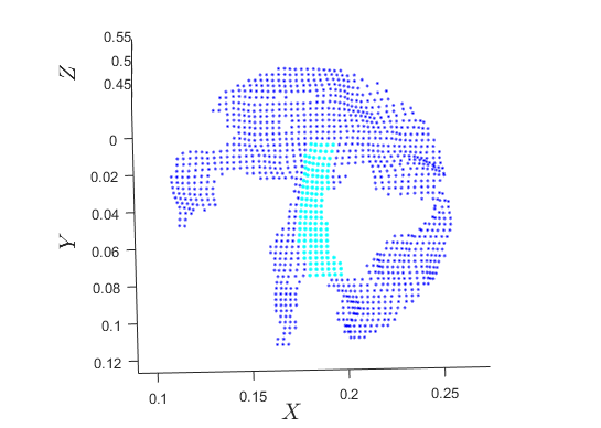
(a) Scene’s point-cloud $\mathcal{W}$. Obstacles subset $\mathcal{O}$: blue. Stem subset $\mathcal{S}$: cyan.

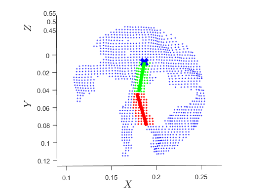
(b) Stem’s point-cloud clustering and line segment fitting: green and red. Stem’s base: blue x.

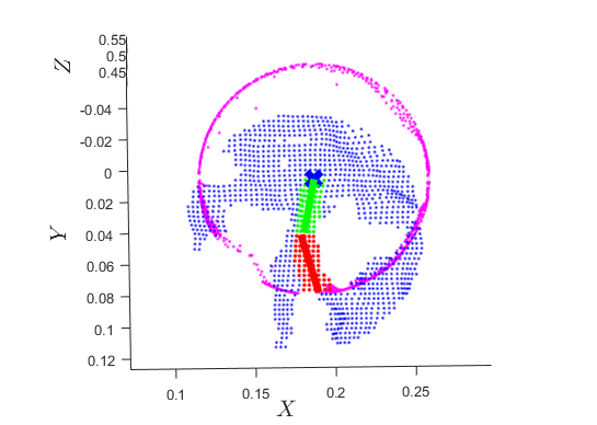
(c) Obstacles projection upon sphere subset $\mathcal{O}_{pr}$: purple.

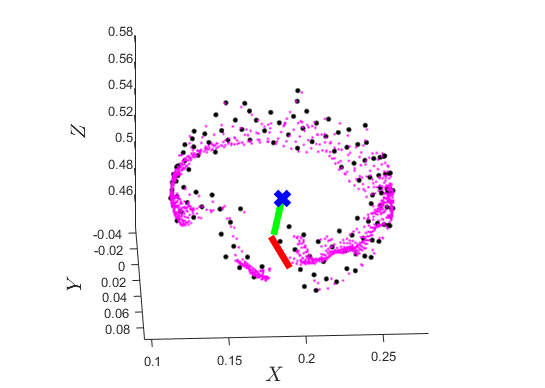
(d) Sphere surface sampling ($500$ samples). Near-obstacles sampled points: black. $\mathcal{O}$ and $\mathcal{S}$ omitted for clarity.

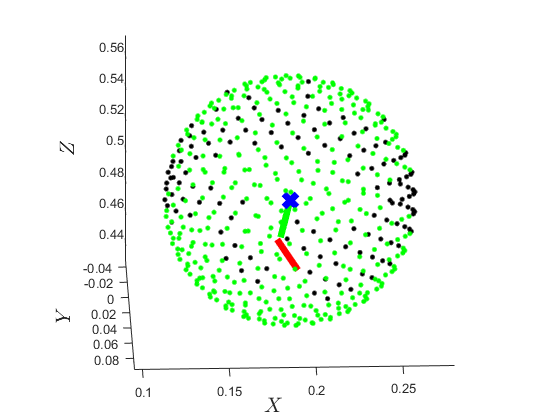
(e) Free-space sphere points: green. Near-obstacles sampled points: black. $\mathcal{O}_{pr}$ omitted for clarity.

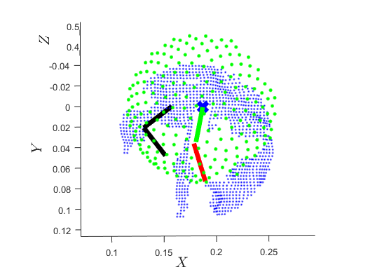
(f) Free-space hemisphere subset $\mathcal{F}$: green. Obstacles $\mathcal{O}$: blue. Plane fitted into $\mathcal{O}$: black lines. Near-obstacles sampled points omitted for clarity.

Figure 2: Point-cloud processing example from lab experimentation with a Real-Sense camera and a mock-up crop. Figures shown from camera’s viewpoint with $Z$ axis corresponding to the camera’s view direction.

Let $\mathcal{W}:\{\mathbf{p}_{w_{i}}\in\mathbb{R}^{3}\ ,\ i=1,...,n_{W}\}$ be the set of $n_{W}\in\mathbb{N}$ points of the point-cloud captured by the camera with $\mathbf{p}_{w_{i}}$ being their position vector expressed in the world frame (Fig. 2(a)). Let subset $\mathcal{S}\subseteq\mathcal{W}:\{\mathbf{p}_{s_{j}}\in\mathbb{R}^{3}\ ,\ j=1,...,n_{S}\}$ denote the detected stem’s point-cloud of $n_{S}\in\mathbb{N}$ points of position $\mathbf{p}_{s_{j}}$ (Fig. 2(a), cyan points). To identify the stem’s base $\mathbf{p}_{sb}\in\mathbb{R}^{3}$, we model the stem by connected linear segments to account for their bending capability. To this end we initially partition $\mathcal{S}$ into separate, consecutive point-cloud clusters, utilizing any of the existing clustering methodologies, e.g. the k-means clustering algorithm. Since crop stems are generally short (e.g. $5-7$ cm), two clusters are considered to be enough to adequately model the stem’s flexibility. We then identify which cluster is further and closer to the grasping arm, comparing the distance between the gripper and each cluster mean value and denote them as ”top” $\mathcal{T}:\{\mathbf{p}_{cl_{a}}\in\mathbb{R}^{3}\ ,\ a=1,...,n_{T}\}$ and ”bottom” $\mathcal{B}:\{\mathbf{p}_{cl_{b}}\in\mathbb{R}^{3}\ ,\ b=1,...,n_{B}\}$ cluster respectively where $\mathbf{p}_{cl_{a}},\ \mathbf{p}_{cl_{b}}$ and $n_{T},n_{B}$ are their respective points’ position vectors and number, with $\mathcal{T},\mathcal{B}\subseteq\mathcal{S}$ and $\mathcal{T}\neq\mathcal{B}$. Utilizing the Principal Component Analysis (PCA), a line segment is fitted into each cluster. Let $\mathbf{n}_{st},\ \mathbf{n}_{sb}\in\mathbb{R}^{3}$ be their direction vectors found by the corresponding major PCA eigenvectors. We can also find the line segments’ length $l_{t},\ l_{b}\in\mathbb{R}_{>0}$ for the top and bottom line respectively, and deduce an estimate of the whole stem’s length $l=l_{t}+l_{b}\in\mathbb{R}_{>0}$.

Point-cloud Subsets	Involved Points
$\text{whole scene}:\mathcal{W}$	$\mathbf{p}_{w_{i}}\in\mathbb{R}^{3}\ ,\ i=1,...,n_{W}$
$\text{stem}:\mathcal{S}\ ,\ \mathcal{S}\subseteq\mathcal{W}$	$\mathbf{p}_{s_{j}}\in\mathbb{R}^{3}\ ,\ j=1,...,n_{S}$
$\text{stem top}:\mathcal{T}\ ,\ \mathcal{T}\subseteq\mathcal{S}$	$\mathbf{p}_{cl_{a}}\in\mathbb{R}^{3}\ ,\ a=1,...,n_{T}$
$\text{stem bottom}:\mathcal{B}\neq\mathcal{T}\ ,\ \mathcal{B}\subseteq\mathcal{S}$	$\mathbf{p}_{cl_{b}}\in\mathbb{R}^{3}\ ,\ b=1,...,n_{B}$
$\text{obstacles}:\noindent\hbox{}$	pok∈R3,k=1,…,nO
proj. obstacles:${\begin{array}[c]{@{}l@{}}\mathcal{O}_{pr}\triangleq\textit{proj}(\mathcal{O})\\ \text{upon}\ \text{S}(\mathbf{p}_{sb},l)\end{array}$}$	projS(pok)∈R3,k=1,…,nO
free-space:F	pfm∈R3,m=1,…,nF