Hierarchical structure of fluctuation theorems for a driven system in contact with multiple heat reservoirs

Abstract

For driven open systems in contact with multiple heat reservoirs, we find the marginal distributions of work or heat do not satisfy any fluctuation theorem, but only the joint distribution of work and heat satisfies a family of fluctuation theorems. A hierarchical structure of these fluctuation theorems is discovered from microreversibility of the dynamics by adopting a step-by-step coarse-graining procedure in both classical and quantum regimes. Thus, we put all fluctuation theorems concerning work and heat into a unified framework. We also propose a general method to calculate the joint statistics of work and heat in the situation of multiple heat reservoirs via the Feynman-Kac equation. For a classical Brownian particle in contact with multiple heat reservoirs, we verify the validity of the fluctuation theorems for the joint distribution of work and heat.

I Introduction

Work and heat are two fundamental quantities in thermodynamics, and usually coexist in generic thermodynamic processes. In stochastic thermodynamics, the definitions of work and heat are extended from ensemble average quantities to trajectory functionals (Jarzynski, 1997a, b; Sekimoto, 1998). A remarkable achievement of the stochastic thermodynamics is the discovery of the fluctuation theorems, which reformulate various versions of the second law of thermodynamics from inequalities into equalities (Seifert, 2008; Esposito et al., 2009; Campisi et al., 2011; Sekimoto, 2010; Jarzynski, 2011; Seifert, 2012; Peliti and Pigolotti, 2021), for example, the Jarzynski equality for work (Jarzynski, 1997a, b), the exchange fluctuation theorem for heat (Jarzynski and Wójcik, 2004), and the fluctuation theorem for entropy production (Crooks, 1999; Seifert, 2005).

Despite the coexistence of work and heat in generic thermodynamic processes, on most occasions the fluctuation theorems of work and those of heat were studied separately in the past. Either the system is in contact with a single reservoir and meanwhile driven by an external agent, or the system is in contact with multiple heat reservoirs but without driving. For the first case, by defining the work as a trajectory functional in stochastic thermodynamics, the work statistics and the nonequilibrium work fluctuation theorems have been extensively studied in various classical systems (Jarzynski, 1997b; Sekimoto, 1998; Mazonka and Jarzynski, 1999; Jarzynski, 2000; Hummer and Szabo, 2001; van Zon and Cohen, 2003; Narayan and Dhar, 2004; Speck and Seifert, 2004; Kawai et al., 2007; Imparato et al., 2007; Maragakis et al., 2008; Sagawa and Ueda, 2010; Speck, 2011; Kwon et al., 2013; Saha and Mukherji, 2014; Holubec et al., 2015; Gong and Quan, 2015; Gong et al., 2016; Hoang et al., 2018; Pagare and Cherayil, 2019; Salazar, 2020; Taniguchi and Cohen, 2007, 2008; Imparato and Peliti, 2006; Then and Engel, 2008; Engel, 2009; Minh and Adib, 2009; Baiesi et al., 2006; Saha et al., 2011; Rana et al., 2014; Saha and Jayannavar, 2008; Li and Tu, 2019; Talkner et al., 2009; Jarzynski, 1997a; Nicolis and Decker, 2017). The nonequilibrium work fluctuation theorems were later extended to the quantum realm based on the two-point measurement definition of the quantum fluctuating work (Kurchan, 2000; Tasaki, 2000; Talkner et al., 2007; Deffner and Lutz, 2008; Andrieux and Gaspard, 2008; Esposito et al., 2009; Campisi et al., 2009, 2011; Hekking and Pekola, 2013; Liu, 2014; Funo and Quan, 2018a). The consistency of the two seemingly unrelated definitions is justified by the quantum-classical correspondence principle for the work statistics (Jarzynski et al., 2015; García-Mata et al., 2017; Brodier et al., 2020; Funo and Quan, 2018a; Zhu et al., 2016; Fei et al., 2018). A hierarchical structure of fluctuation theorems concerning work in the case of a single heat reservoir has been clarified (see the supplemental material of Ref. (Hoang et al., 2018)). For the second case, the heat statistics has been widely explored in various thermal transport models, where the system is usually in contact with multiple heat reservoirs (Saito and Dhar, 2007; Dubi and Di Ventra, 2011; Ren et al., 2010, 2012; Thingna et al., 2012; Wang et al., 2014; Fogedby and Imparato, 2014; Li et al., 2015; Kilgour et al., 2019; Aurell et al., 2020; Santos et al., 2020; Levy and Lostaglio, 2020; Gupta and Sivak, 2021). In the absence of external driving, the system finally reaches a nonequilibrium steady state, where the heat exchange satisfies the exchange fluctuation theorem (Jarzynski and Wójcik, 2004) and/or the Gallavotti-Cohen fluctuation theorem (Gallavotti and Cohen, 1995). The heat statistics has also been studied in relaxation processes in the case of a single heat reservoir but without driving (van Zon and Cohen, 2004; Fogedby and Imparato, 2009; Chatterjee and Cherayil, 2010; Gomez-Solano et al., 2011; Salazar and Lira, 2016; Funo and Quan, 2018b; Imparato et al., 2007; Denzler and Lutz, 2018; Salazar et al., 2019; Fogedby, 2020; Popovic et al., 2021; Pagare and Cherayil, 2019; Paraguassú et al., 2021; Chen et al., 2021; Crisanti et al., 2017). Besides the above two cases, there is the third case. That is, when the system is in contact with multiple heat reservoirs and meanwhile driven by an external agent. In this case, the fluctuation theorems concerning work and/or heat has been largely unexplored so far (but see Refs. (Murashita and Esposito, 2016; Pal et al., 2017; Lee and Park, 2018)).

In this article, we study fluctuation theorems of the third case. The system is weakly coupled to multiple heat reservoirs, and meanwhile is driven by an external agent. We find that in this case the marginal distributions of work or heat do not satisfy any fluctuation theorems. But only the joint distribution of work and heat satisfies a family of fluctuation theorems, which are derived in both classical and quantum regimes. We discover a hierarchical structure of fluctuation theorems for the joint distribution of work and heat from microreversibility (Campisi et al., 2011) of the dynamics by adopting a step-by-step coarse-graining procedure. Thus, we put all fluctuation theorems into a unified framework. This is an exhaustive list of all fluctuation theorems concerning work and heat for a driven system in contact with multiple heat reservoirs. Especially, the Jarzynski equality, the Crooks relation, the exchange fluctuation theorem, and the Clausius inequality can all be recovered under specific conditions. In addition, we also discover some new fluctuation theorems that have not been reported previously.

We also propose a general method to calculate the joint statistics of work and heat via the Feynman-Kac equation, and illustrate this method with a classical Brownian particle in contact with multiple heat reservoirs. For the breathing harmonic oscillator, analytical results of the joint statistics of work and heat are obtained in both the highly underdamped and the overdamped regimes, which recover the known results of work distribution in the highly underdamped and the overdamped regimes (Salazar, 2020; Kwon et al., 2013). Moreover, we can also calculate the joint statistics of work and heat in the generic underdamped regime, which has not been explored so far. The fluctuation theorems for the joint distribution of work and heat are verified through the characteristic function of work and heat.

This article is organized as follows. In Sec. II, we derive a family of fluctuation theorems organized in a hierarchy for the joint distribution of work and heat in the situation of multiple heat reservoirs. These fluctuation theorems can be grouped into three categories, the detailed ones (at the trajectory level), the differential ones (at the distribution level), and the integral ones. In Sec. III, we propose a general method to calculate the joint statistics of work and heat, and illustrate this method with a classical Brownian particle in contact with multiple heat reservoirs. The conclusion is given in Sec. IV.

II Fluctuation theorems of work and heat

As shown in Fig. 1, a system of interest described by the Hamiltonian $H_{S}(\gamma_{S}(t),\lambda(t))$ is in contact with $N$ different heat reservoirs described by the Hamiltonians $H_{\nu}(\gamma_{\nu}(t))$, $1\leq\nu\leq N$, where $\gamma_{S}(t)$ and $\gamma_{\nu}(t)$ denote phase-space points of the system and the $\nu$-th heat reservoir. The external driving $\lambda(t),\;0\leq t\leq\tau$ is only applied to the system. We suppose that we can establish or break the interaction between the system and any of the reservoirs as we choose (Jarzynski, 2000). The initial state of the total system is a product state $\rho_{\mathrm{tot}}^{\mathrm{i}}(\Gamma(0))=\rho_{S}^{\mathrm{i}}(\gamma_{S}(0))\otimes\pi_{1}(\gamma_{1}(0))\otimes...\otimes\pi_{N}(\gamma_{N}(0))$, where $\rho_{S}^{\mathrm{i}}(\gamma_{S}(0))$ is the initial distribution of the system, and $\pi_{\nu}(\gamma_{\nu}(0))=\exp[-\beta_{\nu}H_{\nu}(\gamma_{\nu}(0))]/Z_{\nu}(\beta_{\nu})$ is the canonical distributions of the $\nu$-th heat reservoir with the inverse temperatures $\beta_{\nu}$ and the partition functions $Z_{\nu}(\beta_{\nu})$.

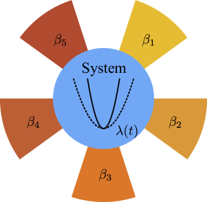
Figure 1: Schematic of an open system under external driving. The system (illustrated as a harmonic oscillator) is in contact with five heat reservoirs simultaneously or sequentially. The inverse temperatures of the heat reservoirs are $\beta_{\nu}$, $\nu=1,2,...,5$. The external driving is depicted by the change of the frequency $\lambda(t)$ of the harmonic potential.

For the classical dynamics, the state of the total system at time $t$ is represented by a point $\Gamma(t)$ in the phase space. An arbitrary trajectory is denoted as $\Gamma=(\gamma_{S},\gamma_{1},...,\gamma_{N})$, where $\gamma_{S}=(x_{S},p_{S})$ and $\gamma_{\nu}=(x_{\nu},p_{\nu})$ with the position $x$ and the momentum $p$ are the trajectories of the system and the $\nu$-th heat reservoir. For a specific external driving $\lambda(t)$, the deterministic trajectory $\Gamma_{\mathrm{d}}$ is fully determined by the initial condition $\Gamma(0)$ of the total system.

Through joint measurements of the internal energies of the system and the heat reservoirs at the beginning and the end (Talkner et al., 2009), the heat exchange with the $\nu$-th heat reservoir along the trajectory $\Gamma$ is given by

$$q_{\nu}(\Gamma)\coloneqq H_{\nu}(\gamma_{\nu}(0))-H_{\nu}(\gamma_{\nu}(\tau)),$$ (1)

and the trajectory work performed by the external driving according to the first law is

$$w(\Gamma)\coloneqq\int_{0}^{\tau}\dot{\lambda}\frac{\partial H_{S}}{\partial\lambda}dt.$$ (2)

We assume the interactions between the system and the heat reservoirs are weak and can be neglected in defining the work and the heat, and the first law holds at the trajectory level by definition (Sekimoto, 1998)

$$H_{S}(\gamma_{S}(\tau),\lambda(\tau))-H_{S}(\gamma_{S}(0),\lambda(0))=w(\Gamma)+\sum_{\nu}q_{\nu}(\Gamma).$$ (3)

In the following, we formulate the fluctuation theorems based on the classical deterministic dynamics. We remark that the following results can be parallel formulated in quantum systems weakly coupled to multiple heat reservoirs (see Appendix A).

II.1 Detailed fluctuation theorems

To formulate the most detailed fluctuation theorem, we define the conditional probability density $\mathcal{P}(\Gamma|\Gamma(0))$ in the trajectory space, where $\Gamma$ can be an arbitrary trajectory (not necessarily the deterministic trajectory $\Gamma_{\mathrm{d}}$ determined by the equation of motion). The deterministic evolution implies $\mathcal{P}(\Gamma|\Gamma(0))$ is nonzero only when $\Gamma=\Gamma_{\mathrm{d}}$. In the reverse process, the trajectory is represented by $\tilde{\Gamma}(t)=\Theta[\Gamma(\tau-t)]$ with the time-reversal operation $\Theta$; the position and the momentum are $\tilde{x}_{S(\nu)}(t)=\Theta[x_{S(\nu)}(\tau-t)]=x_{S(\nu)}(\tau-t)$ and $\tilde{p}_{S(\nu)}(t)=\Theta[p_{S(\nu)}(\tau-t)]=-p_{S(\nu)}(\tau-t)$; the Hamiltonians are $\tilde{H}_{S}(\tilde{\gamma}_{S}(t),\tilde{\lambda}(t))\coloneqq\Theta[H(\gamma_{S}(\tau-t),\lambda(\tau-t))]$ and $\tilde{H}_{\nu}(\tilde{\gamma}_{\nu}(t))\coloneqq\Theta[H(\gamma_{\nu}(\tau-t))]$. The control parameter is assumed to be even parity under the time-reversal operation, and in the reverse process it changes as $\tilde{\lambda}(t)=\lambda(\tau-t)$. As a consequence of microreversibility, the conditional probability density of the trajectory in the reverse process satisfies

$$\tilde{\mathcal{P}}(\tilde{\Gamma}|\tilde{\Gamma}(0))=\mathcal{P}(\Gamma|\Gamma(0)),$$ (4)

which can be regarded as the most detailed fluctuation theorem. Various fluctuation theorems at different levels can be derived from Eq. (4) by adopting a step-by-step coarse-graining procedure.

We also prepare the heat reservoirs in their equilibrium states at the initial time in the reverse processes $\tilde{\pi}_{\nu}(\tilde{\gamma}_{\nu}(0))=\Theta[\pi_{\nu}(\gamma_{\nu}(\tau))]$. For given initial value $\gamma_{\nu}(0)$ and final value $\gamma_{\nu}(\tau)$ of the reservoir trajectories, the conditional probability density of the system trajectory in the forward process is

$$\mathcal{P}_{S}(\gamma_{S};\{\gamma_{\nu}(\tau)\},\{\gamma_{\nu}(0)\}|\gamma_{S}(0))$$

$$\quad\coloneqq\sum_{\{\gamma_{\nu}\}}\mathcal{P}(\gamma_{S},\{\gamma_{\nu}\}|\gamma_{S}(0),\{\gamma_{\nu}(0)\})\prod_{\nu}\pi_{\nu}(\gamma_{\nu}(0)),$$ (5)

where $\mathcal{P}(\gamma_{S},\{\gamma_{\nu}\}|\gamma_{S}(0),\{\gamma_{\nu}(0)\})=\mathcal{P}(\Gamma|\Gamma(0))$, and the summation over the trajectory $\gamma_{\nu}$ of the heat reservoirs, as the path integral, is conditioned on the initial values $\gamma_{\nu}(0)$ and the final values $\gamma_{\nu}(\tau)$. It is similar to define $\mathcal{\tilde{P}}_{S}(\tilde{\gamma}_{S};\{\tilde{\gamma}_{\nu}(\tau)\},\{\tilde{\gamma}_{\nu}(0)\}|\tilde{\gamma}_{S}(0))$ for the reverse process. According to Eq. (4), $\mathcal{\tilde{P}}_{S}$ and $\mathcal{P}_{S}$ are both nonzero simultaneously. Then, we integrate over $\gamma_{\nu}(0)$ and $\gamma_{\nu}(\tau)$ and obtain the coarse-grained conditional probability density $\mathcal{P}_{S}(\gamma_{S};\{q_{\nu}\}|\gamma_{S}(0))\coloneqq\dotsint\prod_{\nu}\{d\gamma_{\nu}(0)d\gamma_{\nu}(\tau)\delta[q_{\nu}-H_{\nu}(\gamma_{\nu}(0))+H_{\nu}(\gamma_{\nu}(\tau))]\}\mathcal{P}_{S}(\gamma_{S};\{\gamma_{\nu}(0)\},\{\gamma_{\nu}(\tau)\}|\gamma_{S}(0))$. The ratio of the probability densities in the reverse and the forward processes is

$$\frac{\mathcal{\tilde{P}}_{S}(\tilde{\gamma}_{S};\{-q_{\nu}\}|\tilde{\gamma}_{S}(0))}{\mathcal{P}_{S}(\gamma_{S};\{q_{\nu}\}|\gamma_{S}(0))}=e^{\sum_{\nu}\beta_{\nu}q_{\nu}}.$$ (6)

Here, $q_{\nu}$ ($-q_{\nu}$) denotes the heat exchange with the $\nu$-th heat reservoir in the forward (reverse) process. Equation (6) can be regarded as the generalization of its single-reservoir version $\mathcal{\tilde{P}}_{S}(\tilde{\gamma}_{S};-q|\tilde{\gamma}_{S}(0))=\mathcal{P}_{S}(\gamma_{S};q|\gamma_{S}(0))\exp(\beta q)$ (Kurchan, 1998; Crooks, 2000; Jarzynski, 2000; Maes and Netočný, 2003; Maes, 2004; Seifert, 2005; Andrieux et al., 2007; Gomez-Marin et al., 2008; Parrondo et al., 2009; Crooks, 2011) to the situation of multiple heat reservoirs, and a coarse-grained version of Eq. (6) has been previously obtained in Ref. (Jarzynski, 2000) (see Eq. (23) therein).

Together with the initial distribution $\rho_{S}^{\mathrm{i}}(\gamma_{S}(0))$ of the system, we obtain the complete trajectory probability density $\mathcal{P}_{S}(\gamma_{S};\{q_{\nu}\})\coloneqq\mathcal{P}_{S}(\gamma_{S};\{q_{\nu}\}|\gamma_{S}(0))\rho_{S}^{\mathrm{i}}(\gamma_{S}(0))$ of observing the system trajectory $\gamma_{S}$ associated with the heat exchange $q_{\nu}$ with the $\nu$-th heat reservoir. The ratio of the complete trajectory probability densities is

$$\frac{\mathcal{\tilde{P}}_{S}(\tilde{\gamma}_{S};\{-q_{\nu}\})}{\mathcal{P}_{S}(\gamma_{S};\{q_{\nu}\})}=e^{\sum_{\nu}\beta_{\nu}q_{\nu}}\frac{\tilde{\rho}_{S}^{\mathrm{i}}(\tilde{\gamma}_{S}(0))}{\rho_{S}^{\mathrm{i}}(\gamma_{S}(0))},$$ (7)

The initial distributions $\rho_{S}^{\mathrm{i}}(\gamma_{S}(0))$ and $\tilde{\rho}_{S}^{\mathrm{i}}(\tilde{\gamma}_{S}(0))$ of the system can be arbitrarily chosen. By choosing the equilibrium states at the inverse temperature $\beta_{S}$ as the initial distributions $\rho_{S}^{\mathrm{i}}(\gamma_{S}(0))=\pi_{S}^{\mathrm{i}}(\gamma_{S}(0))$ and $\tilde{\rho}_{S}^{\mathrm{i}}(\tilde{\gamma}_{S}(0))=\tilde{\pi}_{S}^{\mathrm{i}}(\tilde{\gamma}_{S}(0))$, we can express the detailed fluctuation theorems concerning work and heat at the trajectory level

$$\frac{\mathcal{\tilde{P}}_{S}(\tilde{\gamma}_{S};\{-q_{\nu}\})}{\mathcal{P}_{S}(\gamma_{S};\{q_{\nu}\})} =e^{-\beta_{S}[w(\gamma_{S})-\Delta F_{S}]+\sum_{\nu}(\beta_{\nu}-\beta_{S})q_{\nu}},$$ (8)

where $\Delta F_{S}=-\ln[Z_{S}^{\mathrm{f}}(\beta_{S})/Z_{S}^{\mathrm{i}}(\beta_{S})]/\beta_{S}$ is the free energy difference of the system. In the classical regime, the work $w(\gamma_{S})$ is solely determined by the system trajectory. The detailed fluctuation theorems (6) and (8) are the fine-grained versions of the differential fluctuation theorems (Jarzynski, 2000; Maragakis et al., 2008).

II.2 Differential fluctuation theorems

By grouping the system trajectories $\gamma_{S}$ according to the work $w$, the initial and final values $\gamma_{S}(0)$ and $\gamma_{S}(\tau)$ of the phase-space points, we obtain the conditional joint distribution $P(w,\{q_{\nu}\},\gamma_{S}(\tau)|\gamma_{S}(0))\coloneqq\sum_{\gamma_{S}}\mathcal{P}_{S}(\gamma_{S};\{q_{\nu}\}|\gamma_{S}(0))\delta(w-\int_{0}^{\tau}\dot{\lambda}\partial_{\lambda}H_{S}dt)$. The same coarse-graining procedure is applied to the reverse process. The ratio of the conditional joint distributions of the reverse and the forward processes follows from Eq. (6) as

$$\frac{\tilde{P}(-w,\{-q_{\nu}\},\tilde{\gamma}_{S}(\tau)|\tilde{\gamma}_{S}(0))}{P(w,\{q_{\nu}\},\gamma_{S}(\tau)|\gamma_{S}(0))}=e^{\sum_{\nu}\beta_{\nu}q_{\nu}}.$$ (9)

Similarly, the complete joint distribution of $w$, $q_{\nu}$, $\gamma_{S}(\tau)$ and $\gamma_{S}(0)$ follows as $P(w,\{q_{\nu}\},\gamma_{S}(\tau),\gamma_{S}(0))\coloneqq\sum_{\gamma_{S}}\mathcal{P}_{S}(\gamma_{S};\{q_{\nu}\})\delta(w-\int_{0}^{\tau}\dot{\lambda}\partial_{\lambda}H_{S}dt)$. Please note that a coarse-grained version of Eq. (9) has been previously obtained in Ref. (Jarzynski, 2000) (see Eq. (4) therein). For initial equilibrium states of the system, the ratio of the complete joint distributions becomes

$$\frac{\tilde{P}(-w,\{-q_{\nu}\},\tilde{\gamma}_{S}(\tau),\tilde{\gamma}_{S}(0))}{P(w,\{q_{\nu}\},\gamma_{S}(\tau),\gamma_{S}(0))}=e^{-\beta_{S}[w-\Delta F_{S}]+\sum_{\nu}(\beta_{\nu}-\beta_{S})q_{\nu}}.$$ (10)

Equations (9) and (10) generalize the results in Refs. (Jarzynski, 2000) and (Maragakis et al., 2008) to the situation of multiple heat reservoirs, respectively. These two differential fluctuation theorems are the most detailed ones that can be verified in experiments (Hoang et al., 2018).

From the complete joint distribution $P(w,\{q_{\nu}\},\gamma_{S}(\tau),\gamma_{S}(0))$, we integrate over the initial and the final phase-space points and obtain the joint distribution of work and heat $P(w,\{q_{\nu}\})\coloneqq\iint d\gamma_{S}(\tau)d\gamma_{S}(0)P(w,\{q_{\nu}\},\gamma_{S}(\tau),\gamma_{S}(0))$. Since the right-hand side of Eq. (10) is independent of the phase-space points, the joint distributions of work and heat in the reverse and the forward processes satisfy a generalized Crooks relation

$$\frac{\tilde{P}(-w,\{-q_{\nu}\})}{P(w,\{q_{\nu}\})}=e^{-\beta_{S}[w-\Delta F_{S}]+\sum_{\nu}(\beta_{\nu}-\beta_{S})q_{\nu}},$$ (11)

We remark that Eq. (11) has been obtained previously in Refs. (Murashita and Esposito, 2016; Pal et al., 2017), and a simplified version for the case of a single heat reservoir has been obtained in Ref. (Talkner et al., 2009). But the fine-grained versions of Eq. (11), Eqs. (6)-(10) have not been reported so far.

By integrating over $\gamma_{S}(0)$, $w$ and $q$ in Eq. (10), we obtain a generalized Hummer-Szabo relation

$$\left.\left\langle e^{-\beta_{S}[w-\Delta F_{S}]+\sum_{\nu}(\beta_{\nu}-\beta_{S})q_{\nu}}\right\rangle\right|_{{}_{\gamma_{S}(\tau)}}=\frac{\tilde{\pi}_{S}^{\mathrm{i}}(\tilde{\gamma}_{S}(0))}{\rho_{S}^{\mathrm{f}}(\gamma_{S}(\tau))},$$ (12)

which generalizes the results in Ref. (Hummer and Szabo, 2001) to the situation of multiple heat reservoirs. Here, $\left.\left\langle\cdot\right\rangle\right|_{\gamma_{S}(\tau)}$ denotes the average being conditioned on the given final value $\gamma_{S}(\tau)$ of the system phase-space point, and the marginal distribution $\rho_{S}^{\mathrm{f}}(\gamma_{S}(\tau))$ is obtained by integrating over other variables in $P(w,\{q_{\nu}\},\gamma_{S}(\tau),\gamma_{S}(0))$.

By integrating over $\gamma_{S}(\tau)$, $w$ and $q$ in Eq. (10), we obtain a generalized Jarzynski equality for an initial $\delta$ distribution

$$\left.\left\langle e^{-\beta_{S}[w-\Delta F_{S}]+\sum_{\nu}(\beta_{\nu}-\beta_{S})q_{\nu}}\right\rangle\right|_{\gamma_{S}(0)}=\frac{\tilde{\rho}_{S}^{\mathrm{f}}(\tilde{\gamma}_{S}(\tau))}{\pi_{S}^{\mathrm{i}}(\gamma_{S}(0))}.$$ (13)

In Refs. (Kawai et al., 2007; Gong and Quan, 2015; Hoang et al., 2018), similar fluctuation theorems were obtained for a single heat reservoir. Here we generalize the results to the situation of multiple heat reservoirs. In Eqs. (12) and (13), $\rho_{S}^{\mathrm{f}}(\gamma_{S}(\tau))$ and $\tilde{\rho}_{S}^{\mathrm{f}}(\tilde{\gamma}_{S}(\tau))$ are the final nonequilibrium distributions in the forward and the reverse processes, respectively.

II.3 Integral fluctuation theorems

According to Eq. (7), we can obtain the integral fluctuation theorem

$$\left\langle e^{\sum_{\nu}\beta_{\nu}q_{\nu}}\frac{\tilde{\rho}_{S}^{\mathrm{i}}(\tilde{\gamma}_{S}(0))}{\rho_{S}^{\mathrm{i}}(\gamma_{S}(0))}\right\rangle=1.$$ (14)

This is a generalization of the unified integral fluctuation theorem (Seifert, 2008) to the situation of multiple heat reservoirs. In case the system is initially prepared in an equilibrium state at the inverse temperature $\beta_{S}$, we can express the integral fluctuation theorem of work and heat as

$$\left\langle e^{-\beta_{S}w+\sum_{\nu}(\beta_{\nu}-\beta_{S})q_{\nu}}\right\rangle=e^{-\beta_{S}\Delta F_{S}},$$ (15)

which can also be obtained from the above differential fluctuation theorems (10)-(13) by integrating over the rest variables (see Fig. 2). We would like to emphasize that previously it was believed that in order to construct a fluctuation theorem for a driven open system, e.g., the Jarzynski equality, the system is required to be initially prepared in an equilibrium state whose temperature is the same as that of the heat reservoir. But in Eq. (15), we loosen this constraint, i.e., the initial temperature of the system can be different from that (those) of the heat reservoir(s). Thus, we extend the Jarzynski equality to a broader domain.

If initially the system has the same inverse temperature as those of the heat reservoirs $\beta_{\nu}=\beta_{S}=\beta$ or the system is isolated from the heat reservoir after the initial preparation, the equality (15) is reduced to the Jarzynski equality $\left\langle\exp(-\beta w)\right\rangle=\exp(-\beta\Delta F_{S})$ (Jarzynski, 1997a). On the other hand, if there is no external driving, the equality (15) is reduced to the exchange fluctuation theorem of heat $\left\langle\exp[\sum_{\nu}(\beta_{\nu}-\beta_{S})q_{\nu}]\right\rangle=1$ (Jarzynski and Wójcik, 2004). From the above analysis we can see that Eq. (15) unifies the Jarzynski equality (Jarzynski, 1997a) and the exchange fluctuation theorem of heat (Jarzynski and Wójcik, 2004). From Jensen’s inequality, the Jarzynski equality and the exchange fluctuation theorem lead to the maximum work principle and Clausius’ statement of the second law (Blundell and Blundell, 2009), respectively (see Fig. 2).

As a self-consistent check, one can derive the Clausius inequality (Blundell and Blundell, 2009) from Eq. (15). From Jensen’s inequality, the integral fluctuation theorem (15) leads to a generalized Clausius inequality $-\beta_{S}\left(\left\langle w\right\rangle+\sum_{\nu}\left\langle q_{\nu}\right\rangle\right)+\sum_{\nu}\beta_{\nu}\left\langle q_{\nu}\right\rangle\leq-\beta_{S}\Delta F_{S}$. In an irreversible cycle considered by Clausius, the free energy difference is zero $\Delta F_{S}=0$ due to $\lambda(\tau)=\lambda(0)$, and the state of the system returns to its initial state at the end of the cycle, i.e., $\left\langle H_{S}(\gamma_{S}(\tau),\lambda(\tau))\right\rangle-\left\langle H_{S}(\gamma_{S}(0),\lambda(0))\right\rangle=\left\langle w\right\rangle+\sum_{\nu}\left\langle q_{\nu}\right\rangle=0$. Under these two constraints, the inequality obtained from the integral fluctuation theorem (15) is reduced to the Clausius inequality $\sum_{\nu}\beta_{\nu}\left\langle q_{\nu}\right\rangle\leq 0$.

We remark that a fluctuation theorem relevant to Eq. (15) expressed by the internal energy change has been experimentally verified quite recently (Gómez et al., 2021). Also, an integral fluctuation theorem for the joint distribution of work and heat was reported for the cyclic operation of heat engines (Sinitsyn, 2011; Campisi, 2014; Chen et al., 2022).

We also notice in Ref. (Jarzynski, 1999) an integral fluctuation theorem is obtained as

$$\left\langle e^{\beta_{S}H_{S}(\gamma_{S}(0),\lambda(0))-\beta_{S}^{\prime}H_{S}(\gamma_{S}(\tau),\lambda(\tau))+\sum_{\nu}\beta_{\nu}q_{\nu}}\right\rangle=\frac{Z_{S}^{\mathrm{f}}(\beta_{S}^{\prime})}{Z_{S}^{\mathrm{i}}(\beta_{S})},$$ (16)

which can be derived from Eq. (14) by choosing $\rho_{S}^{\mathrm{i}}(\gamma_{S}(0))$ and $\tilde{\rho}_{S}^{\mathrm{i}}(\tilde{\gamma}_{S}(0))$ as two equilibrium states with different inverse temperatures $\beta_{S}$ and $\beta_{S}^{\prime}$. Only by setting $\beta_{S}^{\prime}=\beta_{S}$, can the internal energy change in Eq. (16) be rewritten into the combination of work and heat.

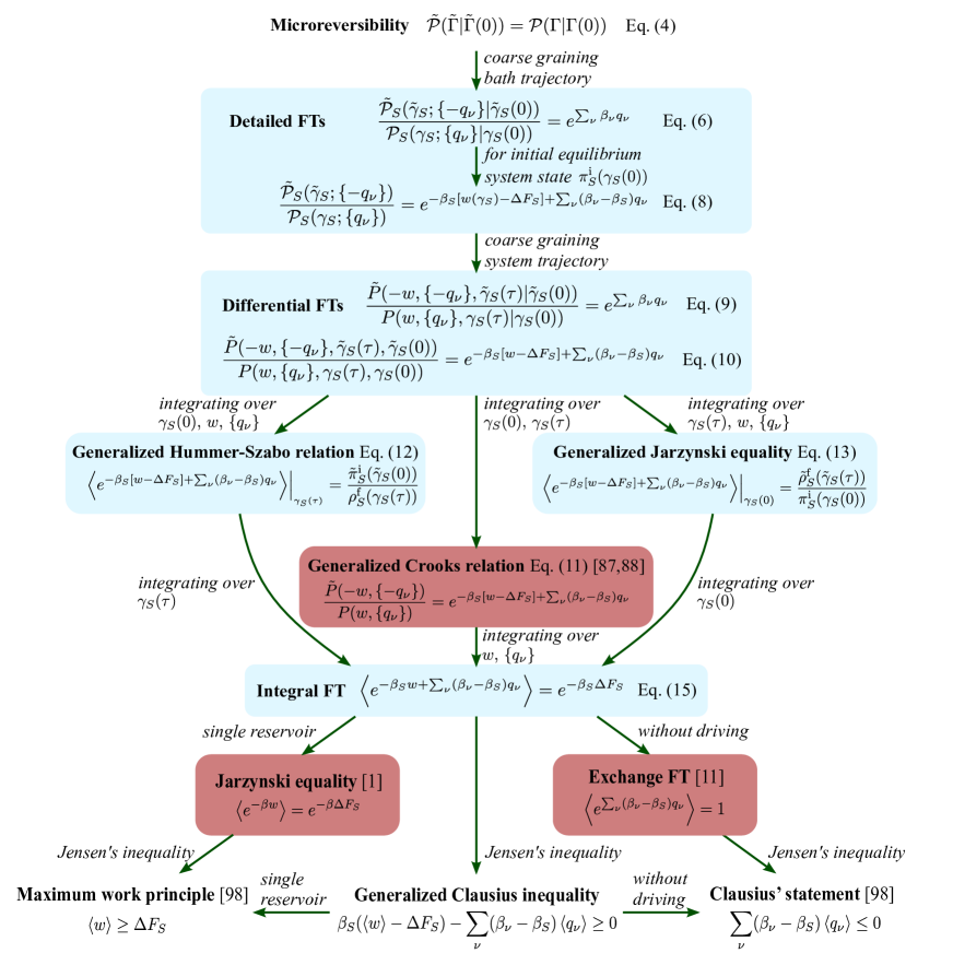
Figure 2: Hierarchical structure of fluctuation theorems (FTs) for a driven system in contact with multiple heat reservoirs. Fluctuation theorems at different levels can be derived from microreversibility (Campisi et al., 2011) of the dynamics by adopting a step-by-step coarse-graining procedure. The fluctuation theorems with red (dark) background have been obtained previously, but these with blue (light) background have not been reported so far. Please note that Eq. (11) has been previously obtained in Refs. (Murashita and Esposito, 2016; Pal et al., 2017), and coarse-grained versions of Eqs. (9) and (6) have been obtained in Ref. (Jarzynski, 2000) (see Eqs. (4) and (23) therein). A similar hierarchical structure of FTs for the work distribution in the situation of a single heat reservoir can be found in the supplemental material of Ref. (Hoang et al., 2018).

The hierarchical structure of fluctuation theorems are summarized in Fig. 2. Figure 2 is an exhaustive list of fluctuation theorems concerning work and heat for a driven system in contact with multiple heat reservoirs. All the fluctuation theorems at different levels can be derived from microreversibility (Campisi et al., 2011) of the dynamics [Eq. (4)] by adopting a step-by-step coarse-graining procedure. The arrows indicate that the fluctuation theorems in lower panels can be derived from those in upper panels after the coarse-graining procedure, but the reverse is not true. From Fig. 2, one can see how the previous known fluctuation theorems (with red (dark) background) and the new fluctuation theorems (with blue (light) background) discovered by us can be fitted into the hierarchical structure of fluctuation theorems. In Appendix A, we parallel formulate a similar hierarchical structure of fluctuation theorems of work and heat in the quantum regime. We remark that the detailed [see Eqs. (6) and (8)] and the differential fluctuation theorems [see Eqs. (9) and (10)] coincide in the quantum regime [see Eqs. (52) and (53)] since a quantum trajectory is defined in the two-point measurement scheme. Generally, several different fluctuation theorems can be ascribed to the fluctuation theorems for entropy production (Crooks, 1999; Seifert, 2005; Yang and Qian, 2020; Manzano et al., 2018; Rao and Esposito, 2018). In Appendix B, we formulate the hierarchical structure of fluctuation theorems for entropy production.

III Joint statistics of work and heat in the situation of multiple heat reservoirs

Recently, the joint distribution of thermodynamic quantities and their associated fluctuation theorems attract more and more attention (Jarzynski, 1999; Talkner et al., 2009; Sinitsyn, 2011; García-García et al., 2012; Campisi, 2014; Murashita and Esposito, 2016; Pal et al., 2017; Miller et al., 2021; Gómez et al., 2021; Denzler et al., 2021; Chen et al., 2022; Lee and Park, 2018). The joint distribution of work and heat is a quantity of significant importance to verify the above fluctuation theorems, but has not been calculated for a nonequilibrium driving process previously. In the following we study the calculation of the joint distribution function of work and heat.

We propose a general method to calculate the joint statistics of work and heat when the system is in contact with multiple heat reservoirs. We would like to emphasize that our method can recover the known results of the work distribution in the highly underdamped and the overdamped regimes (Salazar, 2020; Kwon et al., 2013). Moreover, we can calculate the joint statistics of work and heat in the generic underdamped regime. Our method is illustrated via a classical Brownian particle with mass $m$ moving in a time-dependent potential $\mathcal{U}(x,\lambda(t))$ with the control parameter $\lambda(t)$. We consider the Brownian particle is in contact with multiple heat reservoirs with the inverse temperatures $\beta_{\nu}$ and the friction coefficients $\kappa_{\nu}$. From the point of view of the probability distribution $\rho(x,p,t)$, the stochastic dynamics is described by the Kramers equation (Kramers, 1940)

$$\frac{\partial\rho}{\partial t}=\mathscr{L}\left[\rho\right]+\sum_{\nu}\mathscr{D}_{\nu}\left[\rho\right],$$ (17)

where $\mathscr{L}$ characterizes the deterministic evolution

$$\mathscr{L}\left[\rho\right]=-\frac{\partial}{\partial x}\left(\frac{p}{m}\rho\right)+\frac{\partial}{\partial p}\left(\frac{\partial\mathcal{U}}{\partial x}\rho\right),$$ (18)

and $\mathscr{D}_{\nu}$ characterizes the dissipation induced by the $\nu$-th heat reservoir

$$\mathscr{D}_{\nu}\left[\rho\right]=\frac{\partial}{\partial p}\left(\kappa_{\nu}p\rho+\frac{\kappa_{\nu}m}{\beta_{\nu}}\frac{\partial\rho}{\partial p}\right).$$ (19)

Even through we consider weak coupling between the system and the heat bath, the system-bath interaction can be strong in the classical Brownian motion model, especially in the overdamped situation. Our results are still valid for the classical Brownian motion model. The validity of the Kramers equation (17) is ensured by short bath correlation time, and $\mathcal{U}(x,\lambda(t))$ represents a renormalized potential that the system particle feels (Talkner and Hänggi, 2020). A consistent thermodynamic structure is restored by defining work and heat based on the renormalized system Hamiltonian $H_{S}(x,p,\lambda)=p^{2}/(2m)+\mathcal{U}(x,\lambda)$.

In the following, we study the joint statistics of work and heat for this specific model, and verify the generalized Crooks relation (11) and the integral fluctuation theorem (15).

III.1 Feynman-Kac equation for work and heat

In the classical Brownian motion model, both work and heat are random variables. With the joint distribution of work and heat $P(w,\{q_{\nu}\})$, the characteristic function of work and heat is defined as $\chi^{w,\{q_{\nu}\}}(s,\{u_{\nu}\})\coloneqq\left\langle\exp[i(sw+\sum_{\nu}u_{\nu}q_{\nu})]\right\rangle$. The characteristic function at time $\tau$ can be calculated through

$$\chi^{w,\{q_{\nu}\}}(s,\{u_{\nu}\})=\iint_{-\infty}^{\infty}\eta(x,p,\tau)dxdp,$$ (20)

where $\eta(x,p,t)$ is a distribution function in the phase space depending on the values of $s$ and $u_{\nu}$. The evolution of $\eta(x,p,t)$ is governed by the Feynman-Kac equation (also called the twisted Fokker-Planck equation) (Ren et al., 2012; Liu, 2014)

$$\frac{\partial\eta}{\partial t}=\mathscr{L}\left[\eta\right]+\sum_{\nu}e^{iu_{\nu}H_{S}}\mathscr{D}_{\nu}\left[e^{-iu_{\nu}H_{S}}\eta\right]+is\dot{\lambda}\frac{\partial\mathcal{U}}{\partial\lambda}\eta.$$ (21)

The initial condition is

$$\eta(x,p,0)=\rho(x,p,0)=\frac{e^{-\beta_{S}H_{S}(x,p,\lambda(0))}}{Z_{S}^{\mathrm{i}}(\beta_{S})},$$ (22)

with the partition function $Z_{S}^{\mathrm{i}}(\beta_{S})=\iint_{-\infty}^{\infty}\exp[-\beta_{S}H_{S}(x,p,\lambda(0))]dxdp$ at the initial time. Previously, the Feynman-Kac equation was used to calculate the work statistics and to prove the Jarzynski equality (Hummer and Szabo, 2001).

With the characteristic function, the integral fluctuation theorem (15) can be rewritten as

$$\chi^{w,\{q_{\nu}\}}(i\beta_{S},\{i(\beta_{S}-\beta_{\nu})\})=e^{-\beta_{S}\Delta F_{S}}.$$ (23)

Such an equality can be easily verified by noting that the solution to the Feynman-Kac equation (21) with $s=i\beta_{S}$ and $u_{\nu}=i(\beta_{S}-\beta_{\nu})$ is

$$\eta(x,p,t)=\frac{e^{-\beta_{S}H_{S}(x,p,\lambda(t))}}{Z_{S}^{\mathrm{i}}(\beta_{S})}.$$ (24)

We rewrite the generalized Crooks relation (11) in terms of the characteristic function as

$$\frac{\tilde{\chi}^{w,\{q_{\nu}\}}(-s,\{-u_{\nu}\})}{\chi^{w,\{q_{\nu}\}}(i\beta_{S}+s,\{i(\beta_{S}-\beta_{\nu})+u_{\nu}\})}=e^{\beta_{S}\Delta F_{S}},$$ (25)

where $\tilde{\chi}^{w,\{q_{\nu}\}}(s,\{u_{\nu}\})$ is the characteristic function in the reverse process. The equality (25) can also be proven from the Feynman-Kac equation (21), and the proof is given in Appendix C.

III.2 Example: breathing harmonic oscillator

As an example, we study the joint statistics of work and heat for a Brownian particle in a breathing harmonic potential $\mathcal{U}(x,\lambda(t))=m\lambda^{2}(t)x^{2}/2$, where the control parameter $\lambda(t)$ is the frequency. We consider the situation of a single heat reservoir with the inverse temperature $\beta$ and the friction coefficient $\kappa$. The system is initially prepared in an equilibrium state with the inverse temperature $\beta_{S}$. We would like to emphasize that the extension of the following calculation to multiple heat reservoirs is straightforward.

In this situation, we assume $\eta(x,p,t)$ in a quadratic form

$$\eta(x,p,t)=\frac{\beta_{S}\lambda(0)}{2\pi}e^{-\frac{a}{2}\frac{p^{2}}{m}-\frac{b}{2}m\lambda^{2}(t)x^{2}-c\lambda(t)xp-\Lambda}.$$ (26)

Substituting Eq. (26) into the Feynman-Kac equation (21), we obtain the following set of time-dependent ordinary differential equations

$$\dot{\Lambda} =-\kappa\left(1-\frac{a+iu}{\beta}\right),$$ (27)

$$\dot{a} =2\kappa(a+iu)\left(1-\frac{a+iu}{\beta}\right)-2\lambda(t)c,$$ (28)

$$\dot{b} =2c\left(\lambda(t)-\frac{\kappa}{\beta}c\right)-2\left(b+is\right)\frac{\dot{\lambda}(t)}{\lambda(t)},$$ (29)

$$\dot{c} =\lambda(t)(a-b)-2\frac{\kappa}{\beta}(a+iu)c+\left(\kappa-\frac{\dot{\lambda}(t)}{\lambda(t)}\right)c.$$ (30)

The initial conditions are $\Lambda(0)=0$, $a(0)=\beta_{S}$, $b(0)=\beta_{S}$ and $c(0)=0$ according to Eq. (22). The characteristic function of work and heat follows from Eq. (20) as

$$\chi^{w,q}(s,u) =\frac{\lambda(0)}{\lambda(\tau)}\frac{\beta_{S}e^{-\Lambda(\tau)}}{\sqrt{a(\tau)b(\tau)-c(\tau)^{2}}}.$$ (31)

In the highly underdamped regime $\kappa\ll\lambda(t)$, the dynamics and the work statistics can be calculated with the method of stochastic differential equation of energy (Salazar and Lira, 2016; Salazar, 2020; Chen et al., 2022). For the breathing harmonic oscillator in the highly underdamped regime, the kinetic energy and the potential energy are approximately equal $a\approx b$ (Virial theorem), and the correlation can be neglected $c\approx 0$. The differential Eqs. (27)-(30) can be reduced to

$$\dot{\Lambda} =-\kappa\left(1-\frac{a+iu}{\beta}\right),$$ (32)

$$\dot{a} =\kappa\left(a+iu\right)\left(1-\frac{a+iu}{\beta}\right)-\frac{\dot{\lambda}(t)}{\lambda(t)}\left(a+is\right),$$ (33)

and the characteristic function can be simplified into

$$\chi_{\mathrm{under}}^{w,q}(s,u) =\frac{\lambda(0)}{\lambda(\tau)}\frac{\beta_{S}e^{-\Lambda(\tau)}}{a(\tau)}.$$ (34)

As has been shown previously (Salazar, 2020; Chen et al., 2022), we can even obtain analytical results of the work statistics if we adopt the exponential protocol of the control parameter

$$\lambda(t)=\lambda(0)\exp(\alpha t),$$ (35)

where $\alpha$ is a constant determining the tuning rate of the control parameter. For this protocol, the analytical result of the characteristic function can be obtained as

$$\chi_{\mathrm{under}}^{w,q}(s,u)=\frac{\exp[(\kappa-\alpha)\tau/2]}{\cosh(\Omega\tau)+[\beta\Omega/(\beta_{S}\kappa)-(\alpha\beta-\kappa\beta+2i\kappa u)(\alpha\beta-\kappa\beta+2i\kappa u+2\kappa\beta_{S})/(4\beta\beta_{S}\kappa\Omega)]\sinh(\Omega\tau)},$$ (36)

where $\Omega=\sqrt{(\kappa-\alpha)^{2}/4-i\alpha\kappa(s-u)/\beta}$. The free energy difference is $\Delta F_{S}=\alpha\tau/\beta_{S}$. One can check that the analytical expression (36) satisfies the differential fluctuation theorem (25).

We can similarly consider the overdamped regime. In the overdamped regime $\kappa\gg\lambda(t)$, the relaxation timescales of momentum and position are separated. The relaxation timescale of the momentum is much less than that of the position, and their joint distribution is in a product form $\rho(x,p,t)=\rho_{M}(p)\cdot\hat{\rho}(x,t)$. The momentum distribution $\rho_{M}(p)=\sqrt{\beta/(2\pi m)}\exp[-\beta p^{2}/(2m)]$ is assumed to be the Maxwellian distribution, while the position distribution $\hat{\rho}(x,t)=\int_{-\infty}^{\infty}\rho(x,p,t)dp$ is effectively governed by the Smoluchowski equation $\partial_{t}\hat{\rho}=\hat{\mathscr{D}}[\hat{\rho}]$ due to the separation of the relaxation timescales (Smoluchowski, 1916; Bocquet, 1997; Pan et al., 2018). The dissipative operator is

$$\hat{\mathscr{D}}\left[\hat{\rho}\right]=\frac{1}{m\kappa}\frac{\partial}{\partial x}\left(\frac{\partial\mathcal{U}}{\partial x}\hat{\rho}+\frac{1}{\beta}\frac{\partial\hat{\rho}}{\partial x}\right).$$ (37)

Similar to Eq. (20), the characteristic function can be calculated through

$$\hat{\chi}_{\mathrm{over}}^{w,q}(s,u)=\int_{-\infty}^{\infty}\hat{\eta}(x,\tau)dx,$$ (38)

where the distribution function $\hat{\eta}(x,t)$ satisfies the Feynman-Kac equation

$$\frac{\partial\hat{\eta}}{\partial t}=e^{iu\mathcal{U}}\hat{\mathscr{D}}\left[e^{-iu\mathcal{U}}\hat{\eta}\right]+is\dot{\lambda}\frac{\partial\mathcal{U}}{\partial\lambda}\hat{\eta},$$ (39)

with the initial condition

$$\hat{\eta}(x,0)=\hat{\rho}(x,0)=\frac{e^{-\beta_{S}\mathcal{U}(x,\lambda(0))}}{\hat{Z}_{S}^{\mathrm{i}}(\beta_{S})}.$$ (40)

The normalized constant of the initial position distribution is $\hat{Z}_{S}^{\mathrm{i}}(\beta_{S})=\int_{-\infty}^{\infty}\exp[-\beta_{S}\mathcal{U}(x,\lambda(0))]dx$.

We assume the distribution function $\hat{\eta}$ in the quadratic form

$$\hat{\eta}(x,t)=\lambda(0)\sqrt{\frac{\beta_{S}m}{2\pi}}e^{-\frac{\hat{b}}{2}m\lambda^{2}(t)x^{2}-\hat{\Lambda}}.$$ (41)

The Feynman-Kac equation (39) leads to the differential equations

$$\dot{\hat{\Lambda}} =-\frac{\lambda^{2}(t)}{\kappa}\left(1-\frac{\hat{b}+iu}{\beta}\right),$$ (42)

$$\dot{\hat{b}} =2\frac{\lambda^{2}(t)}{\kappa}\left(\hat{b}+iu\right)\left(1-\frac{\hat{b}+iu}{\beta}\right)-2\frac{\dot{\lambda}(t)}{\lambda(t)}(\hat{b}+is).$$ (43)

The characteristic function is simplified into

$$\hat{\chi}_{\mathrm{over}}^{w,q}(s,u) =\frac{\lambda(0)}{\lambda(\tau)}\sqrt{\frac{\beta_{S}}{\hat{b}(\tau)}}e^{-\hat{\Lambda}(t)}.$$ (44)

It is worth mentioning that in the overdamped regime neglecting the momentum degree of freedom does not affect the work statistics (Pan et al., 2018), but indeed affects to the heats statistics (Murashita and Esposito, 2016; Chen et al., 2021; Paraguassú et al., 2022). To be consistent with Eq. (31), we supplement the contribution from the momentum degree of freedom (fast thermalization at the initial time) to the characteristic function

$$\chi_{\mathrm{over}}^{w,q}(s,u)=\frac{\hat{\chi}_{\mathrm{over}}^{w,q}(s,u)}{\sqrt{(1-\frac{iu}{\beta})(1+\frac{iu}{\beta_{S}})}}.$$ (45)

We will compare Eq. (45) with the exact result [Eq. (31)] in the overdamped regime in the next subsection.

Similar to the highly underdamped regime, we can even obtain analytical results of the characteristic function under some specific protocols of the control parameter. For example, we choose the protocol (Kwon et al., 2013)

$$\lambda(t)=\frac{\lambda(0)}{\sqrt{1+\epsilon t}},$$ (46)

where $\epsilon$ is a constant determining the tuning rate. The analytical result of the characteristic function can be obtained as

$$\chi_{\mathrm{over}}^{w,q}(s,u)=\frac{(1+\epsilon\tau)^{\frac{\delta+\epsilon}{4\epsilon}}/\sqrt{(1-\frac{iu}{\beta})(1+\frac{iu}{\beta_{S}})}}{\left\{\cosh[\frac{\theta}{\epsilon}\ln(1+\epsilon\tau)]+\sinh[\frac{\theta}{\epsilon}\ln(1+\epsilon\tau)]\left[\frac{\beta}{\beta_{S}}(\frac{\theta}{\delta}-\frac{(\delta+\epsilon)^{2}}{4\theta\delta})+(1+\frac{2iu}{\beta_{S}})\frac{\delta+\epsilon}{2\theta}-\frac{iu\delta}{\beta\theta}(1+\frac{iu}{\beta_{S}})\right]\right\}^{\frac{1}{2}}},$$ (47)

where $\delta=2\lambda^{2}(0)/\kappa$ and $\theta=\sqrt{i(s-u)\delta\epsilon/\beta+(\delta+\epsilon)^{2}/4}$. The free energy difference is $\Delta F_{S}=-[\ln(1+\epsilon\tau)]/(2\beta_{S})$. One can check that the analytical expression (47) satisfies the differential fluctuation theorem (25).

By setting $u=0$ in Eqs. (36) and (47), we recover the known results of the work distribution in the highly underdamped and the overdamped regimes (Salazar, 2020; Kwon et al., 2013). Actually, we can calculate the joint distribution of work and heat in the generic underdamped regime under an arbitrary protocol by numerically solving Eqs. (27)-(30). In that sense, our method substantially extends the range of applicability.

III.3 Joint distribution of work and heat

Previously, either the heat distribution or the work distribution has been calculated for various systems (Imparato et al., 2007; Chatterjee and Cherayil, 2010; Speck, 2011; Kwon et al., 2013; Gong et al., 2016; Denzler and Lutz, 2018; Fogedby and Imparato, 2009; Paraguassú et al., 2021; Saha and Mukherji, 2014), but the joint distribution of work and heat has not been calculated so far. For arbitrary protocols of the control parameter $\lambda(t)$, the results of the characteristic function $\chi^{w,q}(s,u)$ can be numerically calculated via Eqs. (27)-(30). As an example to show the effectiveness of our method, we calculate the joint distribution $P(w,q)$ of work and heat. The joint distribution $P(w,q)$ of work and heat is the inverse Fourier transform of the characteristic function $\chi^{w,q}(s,u)$.

We consider a compression process under the exponential protocol $\lambda(t)=\lambda(0)\exp(\alpha t)$ ($\alpha>0$) in the underdamped regime ($\kappa/\lambda(0)=1/10$) and an expansion process under the specific protocol $\lambda(t)=\lambda(0)/\sqrt{1+\epsilon t}$ ($\epsilon>0$) in the overdamped regime ($\kappa/\lambda(0)=10$). In the numerical calculation, we set the initial frequency $\lambda(0)=1$ and the inverse temperatures $\beta_{S}=\beta=1$, i.e., the system is initially in equilibrium with the heat reservoir. Both $\alpha$ and $\epsilon$ are set to be $0.05$ with the control time $\tau=20$.

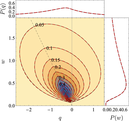
Figure 3: The joint distribution $P(w,q)$ and the marginal distributions $P(w)$ and $P(q)$ at the end $\tau=20$ of the underdamped compression process ($\kappa=0.1$, $\lambda(0)=1$, and $\alpha=0.05$). The black dashed line shows $w=q$. In both the contour map and the marginal distributions, the gray solid (red dashed) contours illustrate the numerical (analytical) results.

Figure 3 illustrates the joint distribution $P(w,q)$ (contour map) of work and heat as well as the marginal distributions, the work distribution $P(w)$ and the heat distribution $P(q)$, at the end $\tau=20$ of the compression process in the underdamped regime ($\kappa=0.1$, $\lambda(0)=1$, and $\alpha=0.05$). The joint distribution $P(w,q)$ is obtained via the two-dimensional discrete inverse Fourier transform of the characteristic function $\chi^{w,q}(s,u)$, where $s$ and $u$ range from $-400$ to $400$ with the interval $0.2$. The red dashed contours are obtained from the analytical expression (36) in the highly underdamped regime, and agree well with the gray solid contours obtained from the exact numerical results. In the marginal distributions, the approximate analytical results (red dashed curves) agree well with the exact numerical results (gray solid curves).

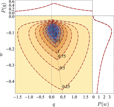
Figure 4: The joint distribution $P(w,q)$ and the marginal distributions $P(w)$ and $P(q)$ at the end $\tau=20$ of the overdamped expansion process ($\kappa=10$, $\lambda(0)=1$, and $\epsilon=0.05$).

Figure 4 illustrates the joint distribution $P(w,q)$ as well as the marginal distributions $P(w)$ and $P(q)$ of work and heat for the expansion process in the overdamped regime ($\kappa=10$, $\lambda(0)=1$, and $\epsilon=0.05$). The heat distribution $P(q)$ is more disperse than the work distribution $P(w)$. In the joint distribution, the agreement between the red dashed contours and the gray solid contours shows the overdamped approximation is perfect under the current parameters. Notice that we have included the contribution from the momentum degree of freedom to the heat statistics in Eq. (45). In the overdamped regime, the thermalization of momentum only contributes to the heat statistics but does not affect the work statistics.

IV Conclusion

In this article, we study the fluctuation theorems when a system is in contact with multiple heat reservoirs and meanwhile is driven by an external agent. In this circumstance, the marginal distributions of work or heat do not satisfy any fluctuation theorem. But only the joint distribution of work and heat satisfies a family of fluctuation theorems. We discover a hierarchical structure of fluctuation theorems for the joint distribution of work and heat in the situation of multiple heat reservoirs (see Fig. 2). This is an exhaustive list of fluctuation theorems concerning work and heat for a driven system in contact with multiple heat reservoirs. We demonstrate how these fluctuation theorems at different levels can be derived from microreversibility (Campisi et al., 2011) of the dynamics by adopting a step-by-step coarse-graining procedure. Thus, we put all fluctuation theorems into a unified framework. From Fig. 2, one can also see how the previously known fluctuation theorems and the new fluctuation theorems discovered by us can be fitted into the hierarchical structure of fluctuation theorems. The Jarzynski equality, the Crooks relation, the exchange fluctuation theorem, and the Clausius inequality can be recovered under specific conditions. The conventional statements of the second law follow from the integral fluctuation theorems by utilizing Jensen’s inequality.

We propose a general method to calculate the joint statistics of work and heat via the Feynman-Kac equation. The joint distribution of work and heat encodes more detailed information of the nonequilibrium driving processes compared to the marginal distributions of work or heat. We exemplify our method with a classical Brownian particle moving in a time-dependent potential, and obtain explicit results of the joint distribution of work and heat for the breathing harmonic oscillator. For the classical Brownian motion model, the system-bath interaction can be strong, and a consistent thermodynamic structure is restored by defining work and heat based on the renormalized system Hamiltonian (Talkner and Hänggi, 2020). In the highly underdamped and the overdamped regimes, we obtain analytical expressions of the characteristic function of work and heat under some specific protocols, and recover the known results of the work distribution (Salazar, 2020; Kwon et al., 2013). In addition, we can also calculate the joint statistics of work and heat in the generic underdamped regime, which has not been reported previously.

The general method can be further employed to study many other problems in stochastic thermodynamics, for example, to evaluate the work and the heat statistics in shortcuts to isothermality (Martínez et al., 2016; Li et al., 2017, 2022; Chen, 2022). Also, it is intriguing to study the joint statistics of work and heat for generic open quantum systems (Liu, 2014; Funo and Quan, 2018a; Salazar, 2020). Extension of our method to calculate the joint distribution of work and heat to driven open quantum systems is left for future exploration.

Appendix A Fluctuation theorems: Quantum setup

In the quantum setup, the Hamiltonians $H_{S}(\lambda(t))$ and $H_{\nu}$ are Hermitian operators. The initial state of the total system is represented by the density matrix $\rho_{\mathrm{tot}}^{\mathrm{i}}=\rho_{S}^{\mathrm{i}}\otimes\pi_{1}\otimes...\otimes\pi_{N}$ in the product form. We consider the initial distribution of the system is also a canonical distribution $\rho_{S}^{\mathrm{i}}=\pi_{S}^{\mathrm{i}}=\sum_{m}p_{S,m}^{\mathrm{i}}\left|m\right\rangle\left\langle m\right|$. The canonical distribution of the $\nu$-th heat reservoir $\pi_{\nu}=\sum_{n_{\nu}}p_{\nu,n_{\nu}}\left|n_{\nu}\right\rangle\left\langle n_{\nu}\right|$. Here, $\left|m\right\rangle$ ($\left|n_{\nu}\right\rangle$) is the eigenstate of the Hamiltonian of the system $H_{S}(\lambda(0))$ (the Hamiltonian of the $\nu$-th heat reservoir $H_{\nu}$), and $p_{S,m}^{\mathrm{i}}$ ($p_{\nu,n_{\nu}}$) is the equilibrium population. The evolution of the total system during the time interval $[0,\tau]$ is given by the unitary evolution $U_{\mathrm{tot}}=\mathrm{T}\exp(-\int_{0}^{\tau}iH_{\mathrm{tot}}(\lambda(t)))$ with the time-ordering operator $\mathrm{T}$ and the total Hamiltonian $H_{\mathrm{tot}}(\lambda(t))=H_{S}(\lambda(t))+\sum_{\nu}H_{\nu}+h_{\mathrm{int}}$. The interaction Hamiltonian $h_{\mathrm{int}}$ is weak and can be neglected when implementing the two-point measurements for work and heat.

We implement the joint measurements of energies over the system and the heat reservoirs at the beginning (end) with the outcomes $E_{S,m}^{\mathrm{i}}$ and $E_{\nu,n_{\nu}}$ ($E_{S,m^{\prime}}^{\mathrm{f}}$ and $E_{\nu,n_{\nu}^{\prime}}$), and obtain the trajectory of the transition $\Gamma=(m,\{n_{\nu}\}\rightarrow m^{\prime},\{n_{\nu}^{\prime}\})$. Here, $E_{S,m}^{\mathrm{i}}$ and $E_{S,m^{\prime}}^{\mathrm{f}}$ are the eigenenergies of the system Hamiltonians $H_{S}(\lambda(0))$ and $H_{S}(\lambda(\tau))$ at the initial and the final time, and $E_{\nu,n_{\nu}}$ is the eigenenergy of the Hamiltonian $H_{\nu}$ of the $\nu$-th heat reservoir. The transition probability is $\mathcal{P}(m^{\prime},\{n_{\nu}^{\prime}\}|m,\{n_{\nu}\})=\left|\left\langle m^{\prime},\{n_{\nu}^{\prime}\}\right|U_{\mathrm{tot}}\left|m,\{n_{\nu}\}\right\rangle\right|^{2}$, where $\left|m,\{n_{\nu}\}\right\rangle$ is the direct product of the eigenstates of the system and the heat reservoirs. The heat exchange with the $\nu$-th heat reservoir is defined by (Talkner et al., 2009)

$$q_{\nu}(\Gamma)\coloneqq E_{\nu,n_{\nu}}-E_{\nu,n_{\nu}^{\prime}}.$$ (48)

The work performed by the external driving, according to the first law, is (Talkner et al., 2009)

$$w(\Gamma)\coloneqq E_{S,m^{\prime}}^{\mathrm{f}}-E_{S,m}^{\mathrm{i}}+\sum_{\nu}(E_{\nu,n_{\nu}^{\prime}}-E_{\nu,n_{\nu}}).$$ (49)

In the quantum setup, microreversibility is guaranteed by the time-reversal invariance of the Hamiltonian

$$H_{\mathrm{tot}}(\lambda(t))\Theta=\Theta H_{\mathrm{tot}}(\lambda(t)),$$ (50)

where $\Theta$ is the quantum mechanical time-reversal (anti-unitary) operator (Andrieux and Gaspard, 2008; Campisi et al., 2011). For the reverse process, the Hamiltonians are associated with the forward ones as $\tilde{H}_{S}(\tilde{\lambda}(t))=\Theta H_{S}(\lambda(\tau-t))\Theta^{\dagger}$ and $\tilde{H}_{\nu}=\Theta H_{\nu}\Theta^{\dagger}$, where the control parameter is tuned as $\tilde{\lambda}(t)=\lambda(\tau-t)$. The initial canonical states are $\tilde{\pi}_{S}^{\mathrm{i}}=\Theta\pi_{S}^{\mathrm{f}}\Theta^{\dagger}=\sum{}_{m^{\prime}}p_{S,m^{\prime}}^{\mathrm{f}}\Theta\left|m^{\prime}\right\rangle\left\langle m^{\prime}\right|\Theta^{\dagger}$ and $\tilde{\pi}_{\nu}=\Theta\pi_{\nu}\Theta^{\dagger}=\sum_{n_{\nu}^{\prime}}p_{\nu,n_{\nu}^{\prime}}\Theta\left|n_{\nu}^{\prime}\right\rangle\left\langle n_{\nu}^{\prime}\right|\Theta^{\dagger}$. The corresponding evolution of the total system is $\tilde{U}_{\mathrm{tot}}=\mathrm{T}\exp(-\int_{0}^{\tau}i\tilde{H}_{\mathrm{tot}}(\tilde{\lambda}(t)))$. The probability of the transition from $\Theta\left|m^{\prime},\{n_{j}^{\prime}\}\right\rangle$ to $\Theta\left|m,\{n_{j}\}\right\rangle$ is $\tilde{\mathcal{P}}(m,\{n_{\nu}\}|m^{\prime},\{n_{\nu}^{\prime}\})=\left|\left\langle m,\{n_{\nu}\}\left|\Theta^{\dagger}\tilde{U}_{\mathrm{tot}}\Theta\right|m^{\prime},\{n_{\nu}^{\prime}\}\right\rangle\right|^{2}$. From Eq. (50), one can verify microreversibility of the evolution $\Theta^{\dagger}\tilde{U}_{\mathrm{tot}}\Theta=U_{\mathrm{tot}}^{\dagger}$. Thus, the transition probabilities of the forward and the reverse processes satisfy

$$\tilde{\mathcal{P}}(m,\{n_{\nu}\}|m^{\prime},\{n_{\nu}^{\prime}\})=\mathcal{P}(m^{\prime},\{n_{\nu}^{\prime}\}|m,\{n_{\nu}\}),$$ (51)

which is the quantum counterpart of Eq. (4).

We prepare the heat reservoirs in their equilibrium states in both the forward and the reverse processes. For the initial state $\left|m\right\rangle$ of the system, the conditional probability of observing the transition $\Gamma$ in the forward process is $\mathcal{P}(m^{\prime},\{n_{\nu}^{\prime}\},\{n_{\nu}\}|m)\coloneqq\mathcal{P}(m^{\prime},\{n_{\nu}^{\prime}\}|m,\{n_{\nu}\})\prod_{\nu}p_{\nu,n_{\nu}}$. We sum over the initial and the final states of the heat reservoirs $\mathcal{P}_{S}(m^{\prime},\{q_{\nu}\}|m)=\sum_{\{n_{\nu}\},\{n_{\nu}^{\prime}\}}\mathcal{P}(m^{\prime},\{n_{\nu}^{\prime}\},\{n_{\nu}\}|m)\delta(q_{\nu}-E_{\nu,n_{\nu}}+E_{\nu,n_{\nu}^{\prime}})$, and obtain

$$\frac{\tilde{\mathcal{P}}_{S}(m,\{-q_{\nu}\}|m^{\prime})}{\mathcal{P}_{S}(m^{\prime},\{q_{\nu}\}|m)}=e^{\sum_{\nu}\beta_{\nu}q_{\nu}}.$$ (52)

Here, $\tilde{\mathcal{P}}_{S}(m,\{-q_{\nu}\}|m^{\prime})$ is similarly defined in the reverse process with the initial state $\Theta\left|m^{\prime}\right\rangle$ of the system. Equation (52) is the quantum counterpart of Eq. (6) or Eq. (9).

Including the initial canonical distribution of the system, we obtain the probability $\mathcal{P}_{S}(m^{\prime},m,\{q_{\nu}\})=\mathcal{P}_{S}(m^{\prime},\{q_{\nu}\}|m)p_{S,m}^{\mathrm{i}}$ of observing the system jumping from $m$ to $m^{\prime}$ with the heat exchange $q_{\nu}$. The ratio of probabilities becomes

$$\frac{\tilde{\mathcal{P}}_{S}(m,m^{\prime},\{-q_{\nu}\})}{\mathcal{P}_{S}(m^{\prime},m,\{q_{\nu}\})}=e^{-\beta_{S}[w(\Gamma)-\Delta F_{S}]+\sum_{\nu}(\beta_{\nu}-\beta_{S})q_{\nu}}.$$ (53)

This is the quantum counterpart of Eq. (8) or Eq. (10). By summing over the initial and the final states of the system $P(w,\{q_{\nu}\})=\sum_{m,m^{\prime}}\mathcal{P}_{S}(m^{\prime},m,\{q_{\nu}\})\delta(w+\sum_{\nu}q_{\nu}-E_{S,m^{\prime}}^{\mathrm{f}}+E_{S,m}^{\mathrm{i}})$, it can be verified that the ratio $\tilde{P}(-w,\{-q_{\nu}\})/P(w,\{q_{\nu}\})$ also satisfies the generalized Crooks relation (11). It is straightforward to derive the quantum counterparts of the differential and the integral fluctuation theorems (12), (13) and (15).

Appendix B Fluctuation theorems for entropy production

Based on Eq. (7), we formulate fluctuation theorems for entropy production in a hierarchy. The entropy change, similar to work and heat, can also been defined along the trajectory (Seifert, 2005). The entropy change of the $\nu$-th heat reservoir is determined by the heat exchange $\Delta s_{\nu}=-\beta_{\nu}q_{\nu}$, when the heat exchange is much smaller than the internal energy of every heat reservoir. The entropy change of the system is related to the initial and final phase-space points

$$\Delta s_{S}=-\ln\tilde{\rho}_{S}^{\mathrm{i}}(\tilde{\gamma}_{S}(0))+\ln\rho_{S}^{\mathrm{i}}(\gamma_{S}(0)).$$ (54)

The initial distribution $\tilde{\rho}_{S}^{\mathrm{i}}$ in the reverse process can be chosen as the time-reversal of the final distribution in the forward process, i.e., $\tilde{\rho}_{S}^{\mathrm{i}}(\tilde{\gamma}_{S}(0))=\Theta[\rho_{S}^{\mathrm{f}}(\gamma_{S}(\tau))]$. The total entropy change is $\Delta s_{\mathrm{tot}}=\Delta s_{S}+\sum_{\nu}\Delta s_{\nu}$.

Then, the detailed fluctuation theorem (6) can be written as

$$\frac{\mathcal{\tilde{P}}_{S}(\tilde{\gamma}_{S};\{-\Delta s_{\nu}\}|\tilde{\gamma}_{S}(0))}{\mathcal{P}_{S}(\gamma_{S};\{\Delta s_{\nu}\}|\gamma_{S}(0))}=e^{-\sum_{\nu}\Delta s_{\nu}},$$ (55)

where the heat exchanges in the probability densities are replaced by the entropy changes of the heat reservoirs. Together with the initial distribution $\rho_{S}^{\mathrm{i}}(\gamma_{S}(0))$ of the system, we obtain the complete trajectory probability density $\mathcal{P}_{S}(\gamma_{S};\Delta s_{S},\{\Delta s_{\nu}\})=\mathcal{P}_{S}(\gamma_{S};\{\Delta s_{\nu}\}|\gamma_{S}(0))\rho_{S}^{\mathrm{i}}(\gamma_{S}(0))$, where the entropy change of the system is related to the initial and the final phase-space points [Eq. (54)]. Equation (7) can also be written as

$$\frac{\mathcal{\tilde{P}}_{S}(\tilde{\gamma}_{S};-\Delta s_{S},\{-\Delta s_{\nu}\})}{\mathcal{P}_{S}(\gamma_{S};\Delta s_{S},\{\Delta s_{\nu}\})}=e^{-\Delta s_{\mathrm{tot}}}.$$ (56)

Equations (55) and (56) are identical to Eqs. (6) and (7), but are formulated in terms of entropy changes.

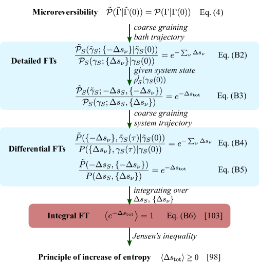
Figure 5: Hierarchical structure of fluctuation theorems for entropy production. Fluctuation theorems at different levels can be derived from microreversibility of the dynamics by adopting a step-by-step coarse-graining procedure. The fluctuation theorem with red (dark) background has been obtained previously, but these with blue (light) background have not been reported so far. To derive these fluctuation theorems, we have assumed the heat exchange is much smaller than the internal energy of every heat reservoir. Please note that Eq. (59) has been previously obtained in Ref. (Jarzynski, 1999) (see Eq. (26) therein), and a coarse-grained version of Eq. (57) has been previously obtained in Ref. (Jarzynski, 2000) (see Eq. (4) therein).

We group the system trajectories according to the entropy changes $\Delta s_{\nu}$ of the heat reservoirs, the initial and final values $\gamma_{S}(0)$ and $\gamma_{S}(\tau)$ of the phase-space points, and obtain the conditional joint distribution $P(\{\Delta s_{\nu}\},\gamma_{S}(\tau)|\gamma_{S}(0))\coloneqq\sum_{\gamma_{S}}\mathcal{P}_{S}(\gamma_{S};\{\Delta s_{\nu}\}|\gamma_{S}(0))$. The differential fluctuation theorem for the conditional joint distribution is obtained from Eq. (55) as

$$\frac{\tilde{P}(\{-\Delta s_{\nu}\},\tilde{\gamma}_{S}(\tau)|\tilde{\gamma}_{S}(0))}{P(\{\Delta s_{\nu}\},\gamma_{S}(\tau)|\gamma_{S}(0))}=e^{-\sum_{\nu}\Delta s_{\nu}}.$$ (57)

Please note that a coarse-grained version of Eq. (57) has been previously obtained in Ref. (Jarzynski, 2000) (see Eq. (4) therein). We can define the joint distribution of entropy changes as $P(\Delta s_{S},\{\Delta s_{\nu}\})\coloneqq\sum_{\gamma_{S}(0),\gamma_{S}(\tau)}P(\{\Delta s_{\nu}\},\gamma_{S}(\tau)|\gamma_{S}(0))\rho_{S}^{\mathrm{i}}(\gamma_{S}(0))\delta[\Delta s_{S}+\ln\rho_{S}^{\mathrm{f}}(\gamma_{S}(\tau))-\ln\rho_{S}^{\mathrm{i}}(\gamma_{S}(0))]$, and obtain the differential fluctuation theorem

$$\frac{\tilde{P}(-\Delta s_{S},\{-\Delta s_{\nu}\})}{P(\Delta s_{S},\{\Delta s_{\nu}\})}=e^{-\Delta s_{\mathrm{tot}}}.$$ (58)

By integrating over $\Delta s_{S}$ and $\Delta s_{\nu}$, it is straightforward to obtain the integral fluctuation theorem

$$\left\langle e^{-\Delta s_{\mathrm{tot}}}\right\rangle=1,$$ (59)

which has been previously obtained in Ref. (Jarzynski, 1999) (see Eq. (26) therein). From Jensen’s inequality, the integral fluctuation theorem (59) leads to the principle of increase of entropy, $\left\langle\Delta s_{\mathrm{tot}}\right\rangle\geq 0$ (Blundell and Blundell, 2009). We illustrate the hierarchical structure of fluctuation theorems for entropy production in Fig. 5.

Appendix C Proof of Eq. (25) based on Kramers equation

We rewrite Eq. (21) as

$$\frac{\partial\eta}{\partial t}=\mathscr{K}_{t}(s,\{u_{\nu}\})\left[\eta\right],$$ (60)

with the time-dependent operator

$$\mathscr{K}_{t}(s,\{u_{\nu}\})\left[\eta\right]=\mathscr{L}\left[\eta\right]+\sum_{\nu}e^{iu_{\nu}H_{S}}\mathscr{D}_{\nu}\left[e^{-iu_{\nu}H_{S}}\eta\right]+is\dot{\lambda}\frac{\partial\mathcal{U}}{\partial\lambda}\eta.$$ (61)

For $\chi^{w,\{q_{\nu}\}}(s+i\beta_{S},\{u_{\nu}+i(\beta_{S}-\beta_{\nu})\})$, the time-dependent operator becomes

$$\mathscr{K}_{t}(s+i\beta_{S},\{u_{\nu}+i(\beta_{S}-\beta_{\nu})\})\left[\eta\right]=\mathscr{L}\left[\eta\right]+\sum_{\nu}e^{\left(iu_{\nu}-\beta_{S}\right)H_{S}}\breve{\mathscr{D}}_{\nu}\left[e^{-\left(iu_{\nu}-\beta_{S}\right)H_{S}}\eta\right]+is\dot{\lambda}\frac{\partial\mathcal{U}}{\partial\lambda}\eta-\beta_{S}\dot{\lambda}\frac{\partial\mathcal{U}}{\partial\lambda}\eta,$$ (62)

where $\breve{\mathscr{D}}_{\nu}$ is defined as

$$\breve{\mathscr{D}}_{\nu}\left[\cdot\right]\coloneqq e^{\beta_{\nu}H_{S}}\mathscr{D}_{\nu}\left[e^{-\beta_{\nu}H_{S}}\cdot\right]=-\kappa_{\nu}p\frac{\partial(\cdot)}{\partial p}+\frac{\kappa_{\nu}m}{\beta_{\nu}}\frac{\partial^{2}(\cdot)}{\partial p^{2}}.$$ (63)

Let us define a new variable $\vartheta(x,p,t)\coloneqq\exp(\beta_{S}H_{S})\eta(x,p,t)$. We rewrite the differential equation (60) associated with the operator (62) as

$$\frac{\partial\vartheta}{\partial t}=\mathscr{L}\left[\vartheta\right]+\sum_{\nu}e^{iu_{\nu}H_{S}}\breve{\mathscr{D}}_{\nu}\left[e^{-iu_{\nu}H_{S}}\vartheta\right]+is\dot{\lambda}\frac{\partial\mathcal{U}}{\partial\lambda}\vartheta.$$ (64)

The initial condition is $\vartheta(x,p,0)=1/Z_{S}^{\mathrm{i}}(\beta_{S})$. At the final time $t=\tau$, the characteristic function can be rewritten as

$$\chi^{w,\{q_{\nu}\}}(s+i\beta_{S},\{u_{\nu}+i(\beta_{S}-\beta_{\nu})\})=\iint_{-\infty}^{\infty}e^{-\beta_{S}H_{S}^{\mathrm{f}}}\vartheta(x,p,\tau)dxdp,$$ (65)

where $\vartheta(x,p,t)$ is propagated according to Eq. (64), and the final Hamiltonian is $H_{S}^{\mathrm{f}}=H_{S}(x,p,\lambda(\tau))$. One can instead consider the corresponding propagation over $\exp(-\beta_{S}H_{S}^{\mathrm{f}})$. We rewrite $\vartheta(x,p,\tau)=\mathscr{U}_{\tau}[\vartheta(x,p,0)]$, which is propagated by the evolution operator $\mathscr{U}_{\tau}$ generated by Eq. (64). For the integral $\iint_{-\infty}^{\infty}\varphi(x,p,\tau)\mathscr{U}_{\tau}[\vartheta(x,p,0)]dxdp$, the conjugate evolution operator $\mathscr{U}_{\tau}^{\dagger}$ on $\varphi(x,p,\tau)$ satisfies

$$\iint_{-\infty}^{\infty}\varphi(x,p,\tau)\mathscr{U}_{\tau}[\vartheta(x,p,0)]dxdp=\iint_{-\infty}^{\infty}\mathscr{U}_{\tau}^{\dagger}(\varphi(x,p,\tau))\vartheta(x,p,0)dxdp.$$ (66)

In the following, we will show the right-hand side of Eq. (66) corresponds to the evolution in the reverse process, and thus prove Eq. (25).

The deterministic evolution satisfies

$$\iint_{-\infty}^{\infty}\varphi\mathscr{L}\left[\vartheta\right]dxdp =\iint_{-\infty}^{\infty}\left(\frac{p}{m}\vartheta\right)\frac{\partial\varphi}{\partial x}-\left(\frac{\partial\mathcal{U}}{\partial x}\vartheta\right)\frac{\partial\varphi}{\partial p}dxdp$$ (67)

$$=\iint_{-\infty}^{\infty}\mathscr{L}\left[\Theta(\varphi)\right]\Theta(\vartheta)dxdp.$$ (68)

The dissipation term satisfies

$$\iint_{-\infty}^{\infty}\varphi\breve{\mathscr{D}}_{\nu}\left[\vartheta\right]dxdp =\iint_{-\infty}^{\infty}\left[\kappa_{\nu}\frac{\partial(p\varphi)}{\partial p}+\frac{\kappa_{\nu}m}{\beta_{\nu}}\frac{\partial^{2}\varphi}{\partial p^{2}}\right]\vartheta dxdp$$ (69)

$$=\iint_{-\infty}^{\infty}\mathscr{D}_{\nu}\left[\varphi\right]\vartheta dxdp.$$ (70)

In the reverse process, the control parameter is tuned as $\tilde{\lambda}(t)=\lambda(\tau-t)$. The performed work is rewritten as

$$is\dot{\lambda}\frac{\partial\mathcal{U}}{\partial\lambda}=-is\dot{\tilde{\lambda}}\frac{\partial\mathcal{U}}{\partial\lambda}.$$ (71)

Both the distributions $\exp(-\beta_{S}H_{S})$ and $\vartheta(x,p,t)$ in the phase space are unchanged under the time-reversal operation, namely, $\Theta[\exp(-\beta_{S}H_{S})]=\exp(-\beta_{S}H_{S})$ and $\Theta[\vartheta(x,p,t)]=\vartheta(x,p,t)$. Combing Eqs. (68), (70) and (71), and the facts $\Theta[\vartheta]=\vartheta$ and $\Theta[\varphi]=\varphi$, we obtain the identity relation

$$\iint_{-\infty}^{\infty}\varphi\left(\mathscr{L}\left[\vartheta\right]+\sum_{\nu}e^{iu_{\nu}}\breve{\mathscr{D}}_{\nu}\left[e^{-iu_{\nu}}\vartheta\right]+is\dot{\lambda}\frac{\partial\mathcal{U}}{\partial\lambda}\vartheta\right)dxdp=\iint_{-\infty}^{\infty}\mathscr{\tilde{K}}_{\tau-t}(-s,\{-u_{\nu}\})\left[\varphi\right]\vartheta dxdp.$$ (72)

Therefore, the propagation over $\vartheta$ in Eq. (65) can be replaced by the propagation over $\exp(-\beta_{S}H_{S}^{\mathrm{f}})$ generated by $\mathscr{\tilde{K}}_{\tau-t}(-s,\{-u_{\nu}\})$ in the reverse process, i.e.

$$\iint_{-\infty}^{\infty}e^{-\beta_{S}H_{S}^{\mathrm{f}}}\vartheta(x,p,\tau)dxdp=\frac{Z_{S}^{\mathrm{f}}(\beta_{S})}{Z_{S}^{\mathrm{i}}(\beta_{S})}\iint_{-\infty}^{\infty}\tilde{\eta}(x,p,\tau)dxdp,$$ (73)

where $\tilde{\eta}(x,p,\tau)$ is associated with the characteristic function $\tilde{\chi}^{w,\{q_{\nu}\}}(-s,\{-u_{\nu}\})$ in the reverse process, and the initial condition is $\tilde{\eta}(x,p,\tau)=\exp(-\beta_{S}H_{S}^{\mathrm{f}})/Z_{S}^{\mathrm{f}}(\beta_{S})$. Thus, we prove Eq. (25) based on the Kramers equation.

References

- Jarzynski (1997a) C. Jarzynski, Nonequilibrium Equality for Free Energy Differences, Phys. Rev. Lett. 78, 2690 (1997a).
- Jarzynski (1997b) C. Jarzynski, Equilibrium free-energy differences from nonequilibrium measurements: A master-equation approach, Phys. Rev. E 56, 5018 (1997b).
- Sekimoto (1998) K. Sekimoto, Langevin Equation and Thermodynamics, Prog. Theor. Phys. Suppl. 130, 17 (1998).
- Seifert (2008) U. Seifert, Stochastic thermodynamics: Principles and perspectives, Eur. Phys. J. B 64, 423 (2008).
- Esposito et al. (2009) M. Esposito, U. Harbola, and S. Mukamel, Nonequilibrium fluctuations, fluctuation theorems, and counting statistics in quantum systems, Rev. Mod. Phys. 81, 1665 (2009).
- Campisi et al. (2011) M. Campisi, P. Hänggi, and P. Talkner, Colloquium: Quantum fluctuation relations: Foundations and applications, Rev. Mod. Phys. 83, 771 (2011).
- Sekimoto (2010) K. Sekimoto, Stochastic Energetics (Springer, Berlin, 2010).
- Jarzynski (2011) C. Jarzynski, Equalities and Inequalities: Irreversibility and the Second Law of Thermodynamics at the Nanoscale, Annu. Rev. Condens. Matter Phys. 2, 329 (2011).
- Seifert (2012) U. Seifert, Stochastic thermodynamics, fluctuation theorems and molecular machines, Rep. Prog. Phys. 75, 126001 (2012).
- Peliti and Pigolotti (2021) L. Peliti and S. Pigolotti, Stochastic Thermodynamics (Princeton University Press, Princeton, 2021).
- Jarzynski and Wójcik (2004) C. Jarzynski and D. K. Wójcik, Classical and Quantum Fluctuation Theorems for Heat Exchange, Phys. Rev. Lett. 92, 230602 (2004).
- Crooks (1999) G. E. Crooks, Entropy production fluctuation theorem and the nonequilibrium work relation for free energy differences, Phys. Rev. E 60, 2721 (1999).
- Seifert (2005) U. Seifert, Entropy Production along a Stochastic Trajectory and an Integral Fluctuation Theorem, Phys. Rev. Lett. 95, 040602 (2005).
- Mazonka and Jarzynski (1999) O. Mazonka and C. Jarzynski, Exactly solvable model illustrating far-from-equilibrium predictions, (1999), arXiv:cond-mat/9912121 [cond-mat.stat-mech] .
- Jarzynski (2000) C. Jarzynski, Hamiltonian Derivation of a Detailed Fluctuation Theorem, J. Stat. Phys. 98, 77 (2000).
- Hummer and Szabo (2001) G. Hummer and A. Szabo, Free energy reconstruction from nonequilibrium single-molecule pulling experiments, Proc. Natl. Acad. Sci. U. S. A. 98, 3658 (2001).
- van Zon and Cohen (2003) R. van Zon and E. G. D. Cohen, Stationary and transient work-fluctuation theorems for a dragged Brownian particle, Phys. Rev. E 67, 046102 (2003).
- Narayan and Dhar (2004) O. Narayan and A. Dhar, Reexamination of experimental tests of the fluctuation theorem, J. Phys. A: Math. Gen. 37, 63 (2004).
- Speck and Seifert (2004) T. Speck and U. Seifert, Distribution of work in isothermal nonequilibrium processes, Phys. Rev. E 70, 066112 (2004).
- Kawai et al. (2007) R. Kawai, J. M. R. Parrondo, and C. V. den Broeck, Dissipation: The Phase-Space Perspective, Phys. Rev. Lett. 98, 080602 (2007).
- Imparato et al. (2007) A. Imparato, L. Peliti, G. Pesce, G. Rusciano, and A. Sasso, Work and heat probability distribution of an optically driven Brownian particle: Theory and experiments, Phys. Rev. E 76, 050101(R) (2007).
- Maragakis et al. (2008) P. Maragakis, M. Spichty, and M. Karplus, A Differential Fluctuation Theorem, J. Phys. Chem. B 112, 6168 (2008).
- Sagawa and Ueda (2010) T. Sagawa and M. Ueda, Generalized Jarzynski Equality under Nonequilibrium Feedback Control, Phys. Rev. Lett. 104, 090602 (2010).
- Speck (2011) T. Speck, Work distribution for the driven harmonic oscillator with time-dependent strength: exact solution and slow driving, J. Phys. A: Math. Theor. 44, 305001 (2011).
- Kwon et al. (2013) C. Kwon, J. D. Noh, and H. Park, Work fluctuations in a time-dependent harmonic potential: Rigorous results beyond the overdamped limit, Phys. Rev. E 88, 062102 (2013).
- Saha and Mukherji (2014) B. Saha and S. Mukherji, Work and heat distributions for a Brownian particle subjected to an oscillatory drive, J. Stat. Mech.: Theory Exp. 2014, P08014 (2014).
- Holubec et al. (2015) V. Holubec, M. Dierl, M. Einax, P. Maass, P. Chvosta, and A. Ryabov, Asymptotics of work distribution for a Brownian particle in a time-dependent anharmonic potential, Phys. Scr. T165, 014024 (2015).
- Gong and Quan (2015) Z. Gong and H. T. Quan, Jarzynski equality, Crooks fluctuation theorem, and the fluctuation theorems of heat for arbitrary initial states, Phys. Rev. E 92, 012131 (2015).
- Gong et al. (2016) Z. Gong, Y. Lan, and H. T. Quan, Stochastic Thermodynamics of a Particle in a Box, Phys. Rev. Lett. 117, 180603 (2016).
- Hoang et al. (2018) T. M. Hoang, R. Pan, J. Ahn, J. Bang, H. T. Quan, and T. Li, Experimental Test of the Differential Fluctuation Theorem and a Generalized Jarzynski Equality for Arbitrary Initial States, Phys. Rev. Lett. 120, 080602 (2018).
- Pagare and Cherayil (2019) A. Pagare and B. J. Cherayil, Stochastic thermodynamics of a harmonically trapped colloid in linear mixed flow, Phys. Rev. E 100, 052124 (2019).
- Salazar (2020) D. S. P. Salazar, Work distribution in thermal processes, Phys. Rev. E 101, 030101(R) (2020).
- Taniguchi and Cohen (2007) T. Taniguchi and E. G. D. Cohen, Onsager-Machlup Theory for Nonequilibrium Steady States and Fluctuation Theorems, J. Stat. Phys. 126, 1 (2007).
- Taniguchi and Cohen (2008) T. Taniguchi and E. G. D. Cohen, Inertial Effects in Nonequilibrium Work Fluctuations by a Path Integral Approach, J. Stat. Phys. 130, 1 (2008).
- Imparato and Peliti (2006) A. Imparato and L. Peliti, Fluctuation relations for a driven Brownian particle, Phys. Rev. E 74, 026106 (2006).
- Then and Engel (2008) H. Then and A. Engel, Computing the optimal protocol for finite-time processes in stochastic thermodynamics, Phys. Rev. E 77, 041105 (2008).
- Engel (2009) A. Engel, Asymptotics of work distributions in nonequilibrium systems, Phys. Rev. E 80, 021120 (2009).
- Minh and Adib (2009) D. D. L. Minh and A. B. Adib, Path integral analysis of Jarzynski’s equality: Analytical results, Phys. Rev. E 79, 021122 (2009).
- Baiesi et al. (2006) M. Baiesi, T. Jacobs, C. Maes, and N. S. Skantzos, Fluctuation symmetries for work and heat, Phys. Rev. E 74, 021111 (2006).
- Saha et al. (2011) A. Saha, J. K. Bhattacharjee, and S. Chakraborty, Work probability distribution and tossing a biased coin, Phys. Rev. E 83, 011104 (2011).
- Rana et al. (2014) S. Rana, P. S. Pal, A. Saha, and A. M. Jayannavar, Single-particle stochastic heat engine, Phys. Rev. E 90, 042146 (2014).
- Saha and Jayannavar (2008) A. Saha and A. M. Jayannavar, Nonequilibrium work distributions for a trapped Brownian particle in a time-dependent magnetic field, Phys. Rev. E 77, 022105 (2008).
- Li and Tu (2019) G. Li and Z. C. Tu, Stochastic thermodynamics with odd controlling parameters, Phys. Rev. E 100, 012127 (2019).
- Talkner et al. (2009) P. Talkner, M. Campisi, and P. Hänggi, Fluctuation theorems in driven open quantum systems, J. Stat. Mech. Theory Exp. 2009, P02025 (2009).
- Nicolis and Decker (2017) G. Nicolis and Y. D. Decker, Stochastic Thermodynamics of Brownian Motion, Entropy 19, 434 (2017).
- Kurchan (2000) J. Kurchan, A quantum fluctuation theorem, (2000), arXiv:cond-mat/0007360 [cond-mat.stat-mech] .
- Tasaki (2000) H. Tasaki, Jarzynski relations for quantum systems and some applications, (2000), arXiv:cond-mat/0009244 [cond-mat.stat-mech] .
- Talkner et al. (2007) P. Talkner, E. Lutz, and P. Hänggi, Fluctuation theorems: Work is not an observable, Phys. Rev. E 75, 050102(R) (2007).
- Deffner and Lutz (2008) S. Deffner and E. Lutz, Nonequilibrium work distribution of a quantum harmonic oscillator, Phys. Rev. E 77, 021128 (2008).
- Andrieux and Gaspard (2008) D. Andrieux and P. Gaspard, Quantum Work Relations and Response Theory, Phys. Rev. Lett. 100, 230404 (2008).
- Campisi et al. (2009) M. Campisi, P. Talkner, and P. Hänggi, Fluctuation Theorem for Arbitrary Open Quantum Systems, Phys. Rev. Lett. 102, 210401 (2009).
- Hekking and Pekola (2013) F. W. J. Hekking and J. P. Pekola, Quantum Jump Approach for Work and Dissipation in a Two-Level System, Phys. Rev. Lett. 111, 093602 (2013).
- Liu (2014) F. Liu, Calculating work in adiabatic two-level quantum Markovian master equations: A characteristic function method, Phys. Rev. E 90, 032121 (2014).
- Funo and Quan (2018a) K. Funo and H. T. Quan, Path Integral Approach to Quantum Thermodynamics, Phys. Rev. Lett. 121, 040602 (2018a).
- Jarzynski et al. (2015) C. Jarzynski, H. T. Quan, and S. Rahav, Quantum-Classical Correspondence Principle for Work Distributions, Phys. Rev. X 5, 031038 (2015).
- García-Mata et al. (2017) I. García-Mata, A. J. Roncaglia, and D. A. Wisniacki, Quantum-to-classical transition in the work distribution for chaotic systems, Phys. Rev. E 95, 050102(R) (2017).
- Brodier et al. (2020) O. Brodier, K. Mallick, and A. M. O. de Almeida, Semiclassical work and quantum work identities in Weyl representation, J. Phys. A: Math. Theor. 53, 325001 (2020).
- Zhu et al. (2016) L. Zhu, Z. Gong, B. Wu, and H. T. Quan, Quantum-classical correspondence principle for work distributions in a chaotic system, Phys. Rev. E 93, 062108 (2016).
- Fei et al. (2018) Z. Fei, H. T. Quan, and F. Liu, Quantum corrections of work statistics in closed quantum systems, Phys. Rev. E 98, 012132 (2018).
- Saito and Dhar (2007) K. Saito and A. Dhar, Fluctuation Theorem in Quantum Heat Conduction, Phys. Rev. Lett. 99, 180601 (2007).
- Dubi and Di Ventra (2011) Y. Dubi and M. Di Ventra, Colloquium: Heat flow and thermoelectricity in atomic and molecular junctions, Rev. Mod. Phys. 83, 131 (2011).
- Ren et al. (2010) J. Ren, P. Hänggi, and B. Li, Berry-Phase-Induced Heat Pumping and Its Impact on the Fluctuation Theorem, Phys. Rev. Lett. 104, 170601 (2010).
- Ren et al. (2012) J. Ren, S. Liu, and B. Li, Geometric Heat Flux for Classical Thermal Transport in Interacting Open Systems, Phys. Rev. Lett. 108, 210603 (2012).
- Thingna et al. (2012) J. Thingna, J. L. García-Palacios, and J.-S. Wang, Steady-state thermal transport in anharmonic systems: Application to molecular junctions, Phys. Rev. B 85, 195452 (2012).
- Wang et al. (2014) J.-S. Wang, B. K. Agarwalla, H. Li, and J. Thingna, Nonequilibrium Green’s function method for quantum thermal transport, Front. Phys. 9, 673 (2014).
- Fogedby and Imparato (2014) H. C. Fogedby and A. Imparato, Heat fluctuations and fluctuation theorems in the case of multiple reservoirs, J. Stat. Mech.: Theory Exp. 2014, P11011 (2014).
- Li et al. (2015) S.-W. Li, C. Cai, and C. Sun, Steady quantum coherence in non-equilibrium environment, Ann. Phys. (NY) 360, 19 (2015).
- Kilgour et al. (2019) M. Kilgour, B. K. Agarwalla, and D. Segal, Path-integral methodology and simulations of quantum thermal transport: Full counting statistics approach, J. Chem. Phys. 150, 084111 (2019).
- Aurell et al. (2020) E. Aurell, B. Donvil, and K. Mallick, Large deviations and fluctuation theorem for the quantum heat current in the spin-boson model, Phys. Rev. E 101, 052116 (2020).
- Santos et al. (2020) J. Santos, A. Timpanaro, and G. Landi, Joint Fluctuation Theorems for Sequential Heat Exchange, Entropy 22, 763 (2020).
- Levy and Lostaglio (2020) A. Levy and M. Lostaglio, Quasiprobability Distribution for Heat Fluctuations in the Quantum Regime, PRX Quantum 1, 010309 (2020).
- Gupta and Sivak (2021) D. Gupta and D. A. Sivak, Heat fluctuations in a harmonic chain of active particles, Phys. Rev. E 104, 024605 (2021).
- Gallavotti and Cohen (1995) G. Gallavotti and E. G. D. Cohen, Dynamical ensembles in stationary states, J. Stat. Phys. 80, 931 (1995).
- van Zon and Cohen (2004) R. van Zon and E. G. D. Cohen, Extended heat-fluctuation theorems for a system with deterministic and stochastic forces, Phys. Rev. E 69, 056121 (2004).
- Fogedby and Imparato (2009) H. C. Fogedby and A. Imparato, Heat distribution function for motion in a general potential at low temperature, J. Phys. A: Math. Theor. 42, 475004 (2009).
- Chatterjee and Cherayil (2010) D. Chatterjee and B. J. Cherayil, Exact path-integral evaluation of the heat distribution function of a trapped Brownian oscillator, Phys. Rev. E 82, 051104 (2010).
- Gomez-Solano et al. (2011) J. R. Gomez-Solano, A. Petrosyan, and S. Ciliberto, Heat Fluctuations in a Nonequilibrium Bath, Phys. Rev. Lett. 106, 200602 (2011).
- Salazar and Lira (2016) D. S. P. Salazar and S. A. Lira, Exactly solvable nonequilibrium Langevin relaxation of a trapped nanoparticle, J. Phys. A: Math. Theor. 49, 465001 (2016).
- Funo and Quan (2018b) K. Funo and H. T. Quan, Path integral approach to heat in quantum thermodynamics, Phys. Rev. E 98, 012113 (2018b).
- Denzler and Lutz (2018) T. Denzler and E. Lutz, Heat distribution of a quantum harmonic oscillator, Phys. Rev. E 98, 052106 (2018).
- Salazar et al. (2019) D. S. P. Salazar, A. M. S. Macêdo, and G. L. Vasconcelos, Quantum heat distribution in thermal relaxation processes, Phys. Rev. E 99, 022133 (2019).
- Fogedby (2020) H. C. Fogedby, Heat fluctuations in equilibrium, J. Stat. Mech.: Theory Exp. 2020, 083208 (2020).
- Popovic et al. (2021) M. Popovic, M. T. Mitchison, A. Strathearn, B. W. Lovett, J. Goold, and P. R. Eastham, Quantum Heat Statistics with Time-Evolving Matrix Product Operators, PRX Quantum 2, 020338 (2021).
- Paraguassú et al. (2021) P. V. Paraguassú, R. Aquino, and W. A. M. Morgado, The heat distribution of the underdamped Langevin equation, (2021), arXiv:2102.09115 [cond-mat.stat-mech] .
- Chen et al. (2021) J.-F. Chen, T. Qiu, and H.-T. Quan, Quantum–Classical Correspondence Principle for Heat Distribution in Quantum Brownian Motion, Entropy 23, 1602 (2021).
- Crisanti et al. (2017) A. Crisanti, A. Sarracino, and M. Zannetti, Heat fluctuations of Brownian oscillators in nonstationary processes: Fluctuation theorem and condensation transition, Phys. Rev. E 95, 052138 (2017).
- Murashita and Esposito (2016) Y. Murashita and M. Esposito, Overdamped stochastic thermodynamics with multiple reservoirs, Phys. Rev. E 94, 062148 (2016).
- Pal et al. (2017) P. S. Pal, S. Lahiri, and A. M. Jayannavar, Transient exchange fluctuation theorems for heat using a Hamiltonian framework: Classical and quantum regimes, Phys. Rev. E 95, 042124 (2017).
- Lee and Park (2018) J. S. Lee and H. Park, Stochastic thermodynamics and hierarchy of fluctuation theorems with multiple reservoirs, New J. Phys. 20, 083010 (2018).
- Kurchan (1998) J. Kurchan, Fluctuation theorem for stochastic dynamics, J. Phys. A: Math. Gen. 31, 3719 (1998).
- Crooks (2000) G. E. Crooks, Path-ensemble averages in systems driven far from equilibrium, Phys. Rev. E 61, 2361 (2000).
- Maes and Netočný (2003) C. Maes and K. Netočný, Time-reversal and entropy, J. Stat. Phys. 110, 269 (2003).
- Maes (2004) C. Maes, in Poincaré Seminar 2003, Vol. 2 (Birkhäuser Basel, 2004) p. 29.
- Andrieux et al. (2007) D. Andrieux, P. Gaspard, S. Ciliberto, N. Garnier, S. Joubaud, and A. Petrosyan, Entropy Production and Time Asymmetry in Nonequilibrium Fluctuations, Phys. Rev. Lett. 98, 150601 (2007).
- Gomez-Marin et al. (2008) A. Gomez-Marin, J. M. R. Parrondo, and C. V. den Broeck, The “footprints” of irreversibility, Europhys. Lett. 82, 50002 (2008).
- Parrondo et al. (2009) J. M. R. Parrondo, C. V. den Broeck, and R. Kawai, Entropy production and the arrow of time, New J. Phys. 11, 073008 (2009).
- Crooks (2011) G. E. Crooks, On thermodynamic and microscopic reversibility, J. Stat. Mech.: Theory Exp. 2011, P07008 (2011).
- Blundell and Blundell (2009) S. J. Blundell and K. M. Blundell, Concepts in Thermal Physics (Oxford University Press, 2009).
- Gómez et al. (2021) S. H. Gómez, N. Staudenmaier, M. Campisi, and N. Fabbri, Experimental test of fluctuation relations for driven open quantum systems with an NV center, New J. Phys. 23, 065004 (2021).
- Sinitsyn (2011) N. A. Sinitsyn, Fluctuation relation for heat engines, J. Phys. A: Math. Theor. 44, 405001 (2011).
- Campisi (2014) M. Campisi, Fluctuation relation for quantum heat engines and refrigerators, J. Phys. A. 47, 245001 (2014).
- Chen et al. (2022) Y. H. Chen, J.-F. Chen, Z. Fei, and H. T. Quan, Microscopic theory of the Curzon-Ahlborn heat engine based on a Brownian particle, Phys. Rev. E 106, 024105 (2022).
- Jarzynski (1999) C. Jarzynski, Microscopic analysis of Clausius-Duhem processes, J. Stat. Phys. 96, 415 (1999).
- Yang and Qian (2020) Y.-J. Yang and H. Qian, Unified formalism for entropy production and fluctuation relations, Phys. Rev. E 101, 022129 (2020).
- Manzano et al. (2018) G. Manzano, J. M. Horowitz, and J. M. R. Parrondo, Quantum Fluctuation Theorems for Arbitrary Environments: Adiabatic and Nonadiabatic Entropy Production, Phys. Rev. X 8, 031037 (2018).
- Rao and Esposito (2018) R. Rao and M. Esposito, Detailed Fluctuation Theorems: A Unifying Perspective, Entropy 20, 635 (2018).
- García-García et al. (2012) R. García-García, V. Lecomte, A. B. Kolton, and D. Domínguez, Joint probability distributions and fluctuation theorems, J. Stat. Mech.: Theory Exp. 2012, P02009 (2012).
- Miller et al. (2021) H. J. D. Miller, M. H. Mohammady, M. Perarnau-Llobet, and G. Guarnieri, Joint statistics of work and entropy production along quantum trajectories, Phys. Rev. E 103, 052138 (2021).
- Denzler et al. (2021) T. Denzler, J. F. G. Santos, E. Lutz, and R. Serra, Nonequilibrium fluctuations of a quantum heat engine, (2021), arXiv:2104.13427 [quant-ph] .
- Kramers (1940) H. Kramers, Brownian motion in a field of force and the diffusion model of chemical reactions, Physica 7, 284 (1940).
- Talkner and Hänggi (2020) P. Talkner and P. Hänggi, Colloquium: Statistical mechanics and thermodynamics at strong coupling: Quantum and classical, Rev. Mod. Phys. 92, 041002 (2020).
- Smoluchowski (1916) M. V. Smoluchowski, Über Brownsche Molekularbewegung unter Einwirkung äußerer Kräfte und deren Zusammenhang mit der verallgemeinerten Diffusionsgleichung, Ann. Phys. (Berlin) 353, 1103 (1916).
- Bocquet (1997) L. Bocquet, High friction limit of the Kramers equation: The multiple time-scale approach, Am. J. Phys. 65, 140 (1997).
- Pan et al. (2018) R. Pan, T. M. Hoang, Z. Fei, T. Qiu, J. Ahn, T. Li, and H. T. Quan, Quantifying the validity and breakdown of the overdamped approximation in stochastic thermodynamics: Theory and experiment, Phys. Rev. E 98, 052105 (2018).
- Paraguassú et al. (2022) P. V. Paraguassú, R. Aquino, L. Defaveri, and W. A. M. Morgado, Effects of the kinetic energy in heat for overdamped systems, Phys. Rev. E 106, 044106 (2022).
- Martínez et al. (2016) I. A. Martínez, A. Petrosyan, D. Guéry-Odelin, E. Trizac, and S. Ciliberto, Engineered swift equilibration of a Brownian particle, Nat. Phys. 12, 843 (2016).
- Li et al. (2017) G. Li, H. T. Quan, and Z. C. Tu, Shortcuts to isothermality and nonequilibrium work relations, Phys. Rev. E 96, 012144 (2017).
- Li et al. (2022) G. Li, J.-F. Chen, C. P. Sun, and H. Dong, Geodesic Path for the Minimal Energy Cost in Shortcuts to Isothermality, Phys. Rev. Lett. 128, 230603 (2022).
- Chen (2022) J.-F. Chen, Optimizing Brownian heat engine with shortcut strategy, Phys. Rev. E 106, 054108 (2022).