The time evolution of bias

Abstract

We investigate the time evolution of bias of cosmic density fields. We perform numerical simulations of the evolution of the cosmic web for the conventional $\Lambda$ cold dark matter ($\Lambda$CDM) model. The simulations cover a wide range of box sizes $L=256-1024h^{-1}\,{\rm Mpc}$, and epochs from very early moments $z=30$ to the present moment $z=0$. We calculate spatial correlation functions of galaxies, $\xi(r)$, using dark matter particles of the biased $\Lambda$CDM simulation. We analyse how these functions describe biasing properties of the evolving cosmic web. We find that for all cosmic epochs the bias parameter, defined through the ratio of correlation functions of selected samples and matter, depends on two factors: the fraction of matter in voids and in the clustered population, and the luminosity (mass) of galaxy samples. Gravity cannot evacuate voids completely, thus there is always some unclustered matter in voids, thus the bias parameter of galaxies is always greater than unity, over the whole range of evolution epochs. We find that for all cosmic epochs bias parameter values form regular sequences, depending on galaxy luminosity (particle density limit), and decreasing with time.

1 Introduction

The relative distribution of galaxies and mass and its evolution in time is of increasing concern in cosmology. It is well known that galaxies do not trace exactly the mass. The difference in the distribution of mass and galaxies was noticed already by Jõeveer et al. (1978); Jõeveer & Einasto (1978), who found in the distribution of galaxies large almost empty voids, occupying about 98 per cent of the volume of the universe. Authors concluded that since gravity works slowly it is impossible to evacuate such large regions completely – there must be dark matter (DM) in voids. The presence of rarefied matter in voids was demonstrated by early numerical simulations of the evolution of the universe by Doroshkevich et al. (1980); Doroshkevich et al. (1982). The difference between distributions of matter and galaxies was explained by Zeldovich et al. (1982) as an indication of a treshold mechanism in galaxy formation – in low-density regions galaxies cannot form. This phenomenon was described quantitatively by Kaiser (1984), who suggested the term “biasing”. In this paper Kaiser (1984) used biasing to describe the difference in the distribution of galaxies and clusters of galaxies. Novadays this term denotes the relationship between distributions of galaxies of various luminosity (or mass) and that of the mass, including DM.

There exist a very large number of studies devoted to the biasing problem, for a recent review see Desjacques et al. (2018). Most of these studies discuss detailed properties of the distribution of galaxies and matter in the present epoch. There exist only a few studies of the time evolution of the bias. These studies are based either on the perturbation theory of the evolution of the cosmic web, as done by Fry (1996) and Tegmark & Peebles (1998), or on numerical simulation of the evolution of the density field (Dubois et al. (2021), Park et al. (2022)).

Usually the bias is defined through density fields of matter and galaxies: $b=\delta_{g}/\delta_{m}$, where $\delta_{g}=N_{\mathrm{gal}}/\overline{N}-1$ and $\delta_{m}=\rho_{m}/\overline{\rho}-1$ are density contrasts of galaxies and matter (Desjacques et al., 2018). However, as noted by Repp & Szapudi (2019a, b, 2020a, 2020b), this bias model leads to unphysical results, since in voids the galaxy density is zero and density contrast is negative, $\delta_{g}=-1$. To avoid this defect we define the bias function through correlation functions of galaxies and matter, $b^{2}=\xi_{g}/\xi_{m}$, as done in the pioneering work by Kaiser (1984).

So far in bias studies only a few cosmic epochs were considered. To understand the bias phenomenon in a broader cosmological context it is needed to find the relationship between matter and galaxies over a large interval of cosmic epochs. The goal of this study is to investigate the time evolution of bias in a large time interval using numerical simulations of the evolution of the cosmic density field. We assume that the $\Lambda$ cold dark matter ($\Lambda$CDM) model represents the actual universe accurately enough, and that it can be used to investigate the evolution of the structure of the real universe. To study the time evolution of bias we use a set of numerical simulations with number of particles $N_{\mathrm{part}}=512^{3}$ and simulation cube sizes $L_{0}=256,~{}512,~{}1024~{}h^{-1}\,{\rm Mpc}$. These simulations were used earlier by Einasto et al. (2019, 2020, 2021a, 2021b) to investigate various properties of the cosmic web.

The bias analysis with correlation functions can be done using three types of objects: simulation particles, simulated galaxies and real galaxies. The analysis by Einasto et al. (2019, 2020) has shown that all three types of objects yield for the bias function similar results. In the present paper we shall use simulation particles as test objects, this approach gives most accurate correlation functions for a wide interval of particle separations. As done by Einasto et al. (2019), we use a simple biased DM simulation model, and divide matter into a low-density population with no galaxy formation or a population of simulated galaxies below a certain mass limit, and a high-density population of clustered matter, associated with galaxies above the mass limit. For each simulation epoch we use (Eulerian) particle local densities, $\rho$, and label particles with this density value.

We apply a sharp particle-density limit, $\rho_{0}$, to select biased samples of particles. This method to select biased galaxy (particle) models was applied earlier among others by Jensen & Szalay (1986), Einasto et al. (1991), Szapudi & Szalay (1993), and Little & Weinberg (1994). This model to select particles for simulated galaxies is similar to the Ising model, discussed by Repp & Szapudi (2019b, a). Actually galaxy formation is a stochastic process, thus the matter density limit which divides unclustered and clustered matter is fuzzy (Dekel (1998), Dekel & Lahav (1999), Taruya et al. (1999); Taruya & Soda (1999), Tegmark & Bromley (1999)). However, a fuzzy density limit has little influence on properties of correlation functions or power spectra of biased and non-biased samples, as shown by Einasto et al. (2019). Biased model samples include particles with density labels, $\rho\geq\rho_{0}$. These samples are found from the full DM sample by excluding particles of density labels less than the limit $\rho_{0}$. In this way biased model samples mimic observed samples of galaxies, where there are no galaxies fainter than a certain luminosity limit. We use a series of particle-density limits $\rho_{0}$.

The paper is organised as follows. In the following Section we describe numerical simulations used in our study, the calculation of the density fields of simulated samples, and the method to find correlation functions. In Section 3 we describe the evolution of particle densities and of the density field. In Section 4 we describe the evolution of biasing properties of our simulated universe. Sections 5 and 6 present the discussion of results and conclusions.

Table 1: Parameters of simulations

Simulation	$L_{0}$	$\sigma_{8}$	$m_{p}$	$R_{0}$
(1)	(2)	(3)	(4)	(5)
L256	256	0.613	$0.993$	0.5
L512	512	0.641	$7.944$	1.0
L1024	1024	0.646	$63.55$	2.0

Columns give: (1) name of simulation; (2) box size in $h^{-1}\,{\rm Mpc}$; (3) $\sigma_{8}$ (4) mass of a particle in units of $10^{10}h^{-1}M_{\odot}$; and (5) effective smoothing scale $R_{0}$ in units of $h^{-1}\,{\rm Mpc}$.

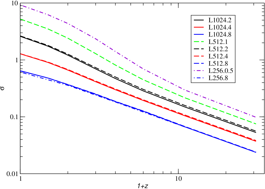
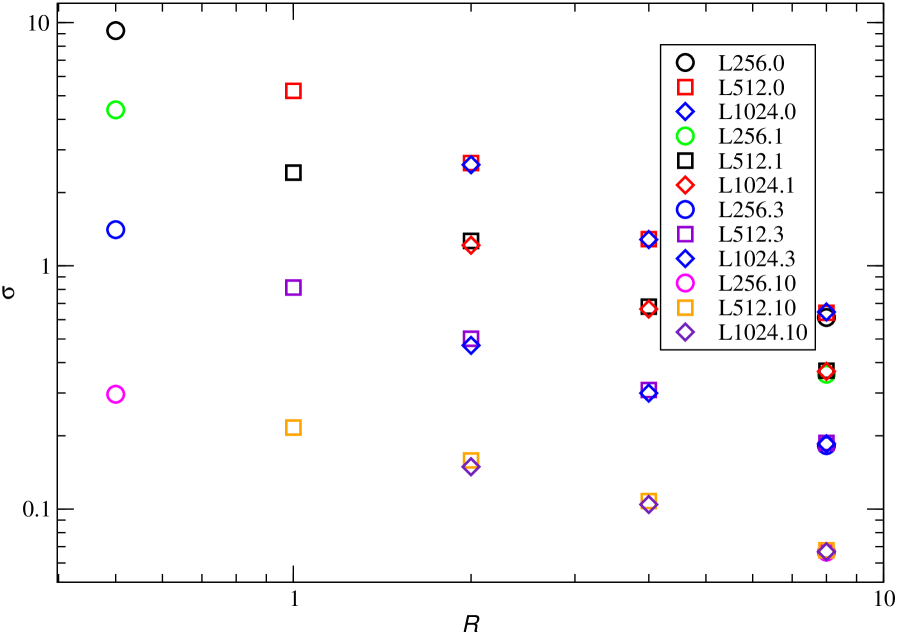
Figure 1: Left: Dependence of the dispersion $\sigma$ of models L256, L512, and L1024 on simulation epoch $z$. The second index in model name shows the smoothing scale $R$ in $h^{-1}\,{\rm Mpc}$. Line types are for models of different size: solid lines for L1024, dashed lines for L512, dotted and dot-dashed lines for L256; colours show smoothing scale: blue for $R=8~{}h^{-1}\,{\rm Mpc}$, red for $R=4~{}h^{-1}\,{\rm Mpc}$, black for $R=2~{}h^{-1}\,{\rm Mpc}$, green for $R=1~{}h^{-1}\,{\rm Mpc}$, and violet for $R=0.5~{}h^{-1}\,{\rm Mpc}$. Right: Dependence of the dispersion $\sigma$ on the smoothing length $R$ of the same models. Here the second index of the model name gives the redshift $z$. The upper sequence of symbols is for the present epoch $z=0$, lower sequences are for redshifts $z=1,~{}3,~{}10$, respectively.

2 Data and methods

In this Section we describe the calculation of simulations and the finding of particle density limited samples, which can be called also as simulated galaxy samples. Then we describe the calculation of density fields and the calculation of correlation and bias functions. We use the value of bias functions at separation $r_{6}=6$ and $r_{10}=10$ as bias parameters.

2.1 Calculation of simulations and biased model samples

We simulated the evolution of the cosmic web adopting a DM $\Lambda$CDM model. We use the GADGET code (Springel, 2005) with three different box sizes $L_{0}=256,~{}512,~{}1024~{}h^{-1}\,{\rm Mpc}$ with $N_{\mathrm{grid}}=512$, and number of particles $N_{\mathrm{part}}=512^{3}$. We call these simulations as L256, L512, and L1024 models. Cosmological parameters for all simulations are ($\Omega_{m},\Omega_{\Lambda},\Omega_{b},h,\sigma_{8},n_{s}$) =(0.28, 0.72, 0.044, 0.693, 0.84, 1.00). Initial conditions were generated using the COSMICS code by Bertschinger (1995), assuming Gaussian fluctuations. Simulations started at redshift $z=30$ using the Zeldovich approximation. We extracted density fields and particle coordinates for eight epochs, corresponding to redshifts $z=30,~{}10,~{}5,~{}3,~{}2,~{}1,~{}0.5,~{}0$. Table LABEL:Tab1 shows parameters of simulations.

For all simulation particles and all simulation epochs, we calculated the local density values at particle locations, $\rho$, using the positions of the 27 nearest particles, including the particle itself. Densities were expressed in units of the mean density of the whole simulation. The full $\Lambda$CDM model includes all particles. Following Einasto et al. (2019), we formed biased model samples that contained particles above a certain limit, $\rho\geq\rho_{0}$, in units of the mean density of the simulation. As shown by Einasto et al. (2019), this sharp density limit allows to find density fields of simulated galaxies, whose geometrical properties are close to the density fields of real galaxies. Thus biased model samples can be called also as simulated galaxy samples or as clustered samples, depending on the context. This method to select particles for simulated galaxies is similar to the Ising model, discussed by Repp & Szapudi (2019b, a). We use a series of particle-density limits $\rho_{0}$ for each simulation epoch. Biased samples are found from the full DM sample by excluding particles with density labels less than the limit $\rho_{0}$. In this way biased model samples mimic observed samples of galaxies, where there are no galaxies fainter than a certain luminosity limit.

The biased samples are denoted LXXX.$i$, where XXX denotes the size of the simulation box in $h^{-1}\,{\rm Mpc}$, and $i$ denotes the particle-density limit $\rho_{0}$. The full DM model includes all particles and corresponds to the particle-density limit $\rho_{0}=0$, therefore it is denoted as LXXX.00. The main data on the model samples are given in Table LABEL:Tab1.

2.2 Calculation of density fields

$N-$body simulations provides us with populations of DM particles in a box of size $L_{0}$ at redshift $z$. The density field was estimated using a filter of size $R_{t}$. The density field was normalised to the average matter density, providing us with the relative density $D(\mathbf{x})$,

$$D(\mathbf{x})=\frac{\rho(\mathbf{x})}{\overline{\rho}},$$ (1)

where $D(\mathbf{x})$ is the density at location $\mathbf{x}$, and ${\overline{\rho}}$ is the mean density. The second moment of the density contrast $\delta(\mathbf{x})=D(\mathbf{x})-1$ is the variance of the density field, $\sigma^{2}$. In the following we call $\sigma$ as the dispersion of the density field.

We determined smoothed density fields of simulations using a $B_{3}$ spline (see Martínez & Saar, 2002),

$$B_{3}(x)=\frac{1}{12}\left[|x-2|^{3}-4|x-1|^{3}+6|x|^{3}-4|x+1|^{3}+|x+2|^{3}\right].$$ (2)

The spline function is different from zero only in the interval $x\in[-2,2]$. To calculate the high-resolution density field we used the kernel of the scale, which is equal to the cell size of the simulation, $L_{0}/N_{\mathrm{grid}}$, where $L_{0}$ is the size of the simulation box and $N_{\mathrm{grid}}$ is the number of grid elements in one coordinate. The smoothing with index $i$ has a smoothing radius $R_{i}=L_{0}/N_{\mathrm{grid}}\times 2^{i}$. The effective scale of smoothing is equal to $2\times R_{i}$. Density fields extracted from simulations have effective smoothing scale $R_{0}=L_{0}/N_{\mathrm{grid}}$. We calculated density fields of models up to smoothing scale $R_{i}=8~{}h^{-1}\,{\rm Mpc}$. The $B_{3}$ kernel of radius $R_{B}=1~{}h^{-1}\,{\rm Mpc}$ corresponds to a Gaussian kernel with dispersion $R_{G}=0.6~{}h^{-1}\,{\rm Mpc}$. For details of the smoothing method see Appendix.A of Einasto et al. (2021a).

2.3 Calculation of the correlation and bias functions

The $\Lambda$CDM model samples contain all particles with local density labels $\rho\geq\rho_{0}$. To derive correlation functions of these samples, a conventional methods (Landy & Szalay, 1993) cannot be used because the number of particles is too large, up to $512^{3}$ in the full unbiased model. To determine the correlation functions we used the Szapudi et al. (2005) method. This method uses the FFT to calculate correlation functions and scales as $O(N\log N)$. The method is an implementation of the algorithm eSpICE, the Euclidean version of SpICE by Szapudi et al. (2001). To find the dependence of results on the size of the grid we calculated correlation functions with two sizes of the grid, $N_{\mathrm{grid}}=2048^{3}$ and $N_{\mathrm{grid}}=1024^{3}$. The finer grid allows to see better the shape of correlation functions and its derivatives on halo scales, the coarse grid allows to suppress wiggles of the correlation functions on large separations. For the finer grid correlation functions were found up to separations $r_{max}=204~{}h^{-1}\,{\rm Mpc}$ to $r_{max}=290~{}h^{-1}\,{\rm Mpc}$ with 308 logarithmic bins for models L256 to L1024. For the $N_{\mathrm{grid}}=1024^{3}$ grid we calculated correlation functions up to separation $r_{max}=64~{}h^{-1}\,{\rm Mpc}$, $r_{max}=127~{}h^{-1}\,{\rm Mpc}$ and $r_{max}=255~{}h^{-1}\,{\rm Mpc}$ for models L256, L512 and L1024, using 128 linear bins. The analysis of both sets of correlation and bias functions showed that wiggles of both functions found with the $N_{\mathrm{grid}}=2048^{3}$ grid are too large for reliable determination of bias parameters, thus in the following we use only results obtained with the $N_{\mathrm{grid}}=1024^{3}$ grid.

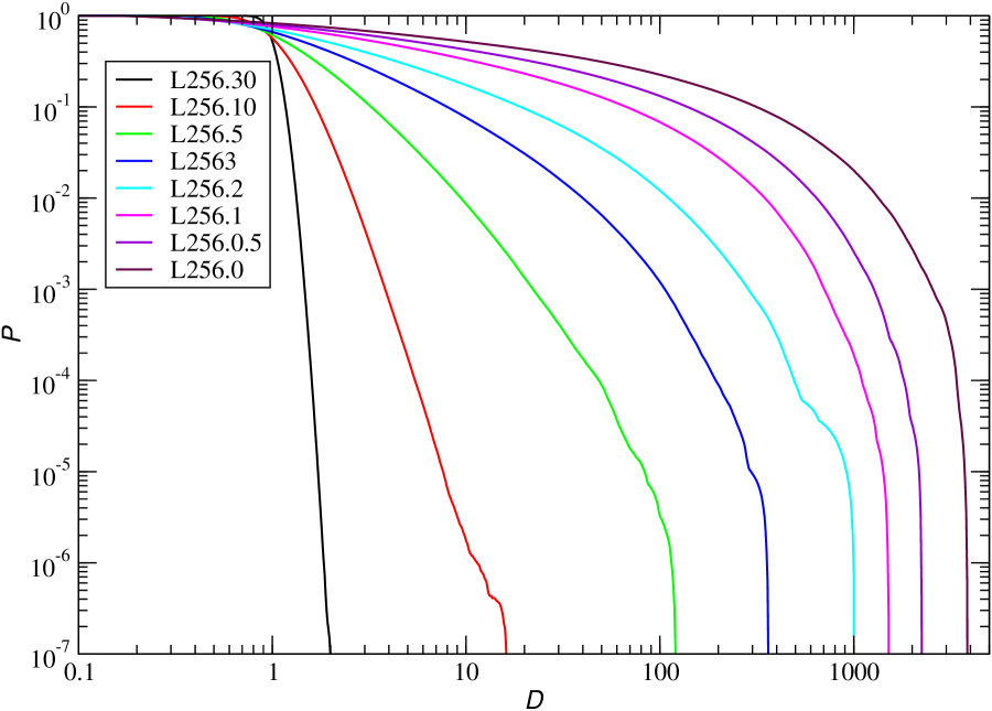
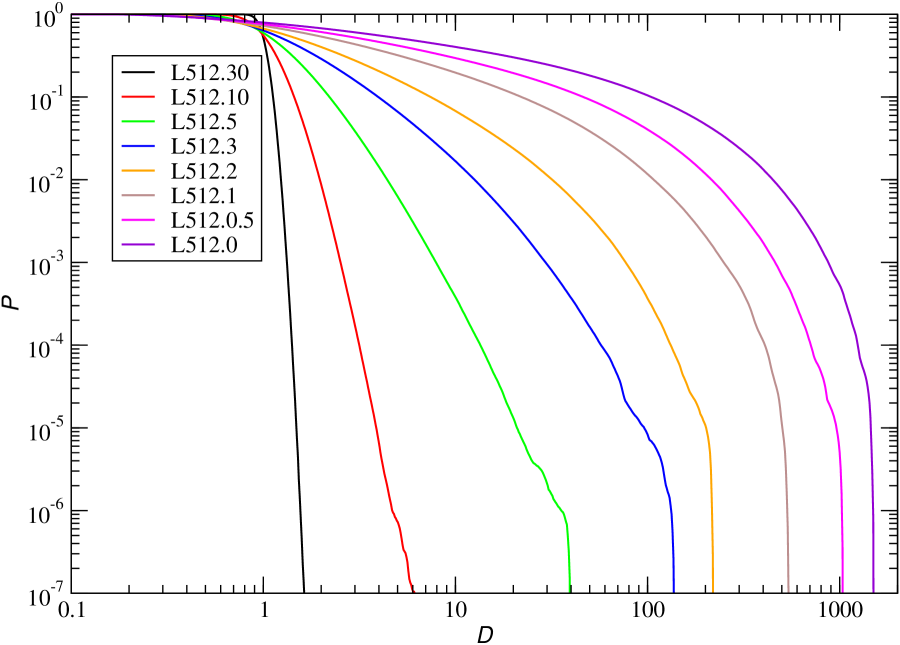
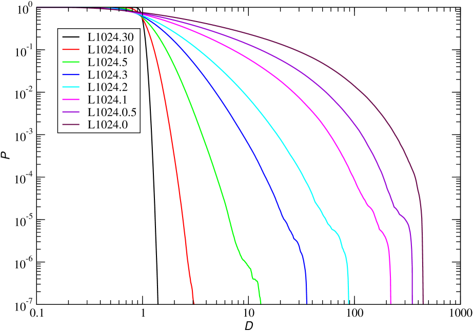
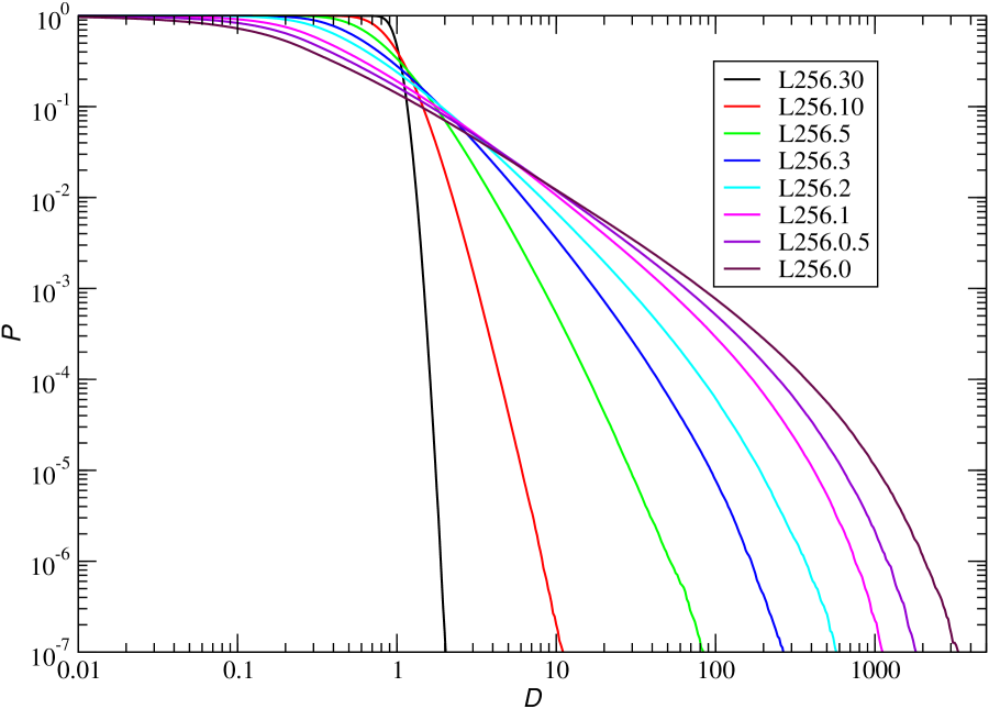
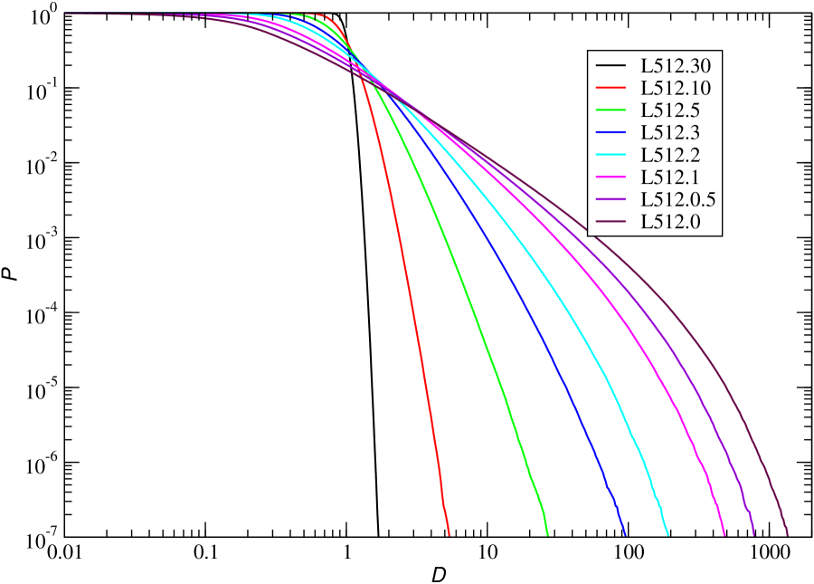
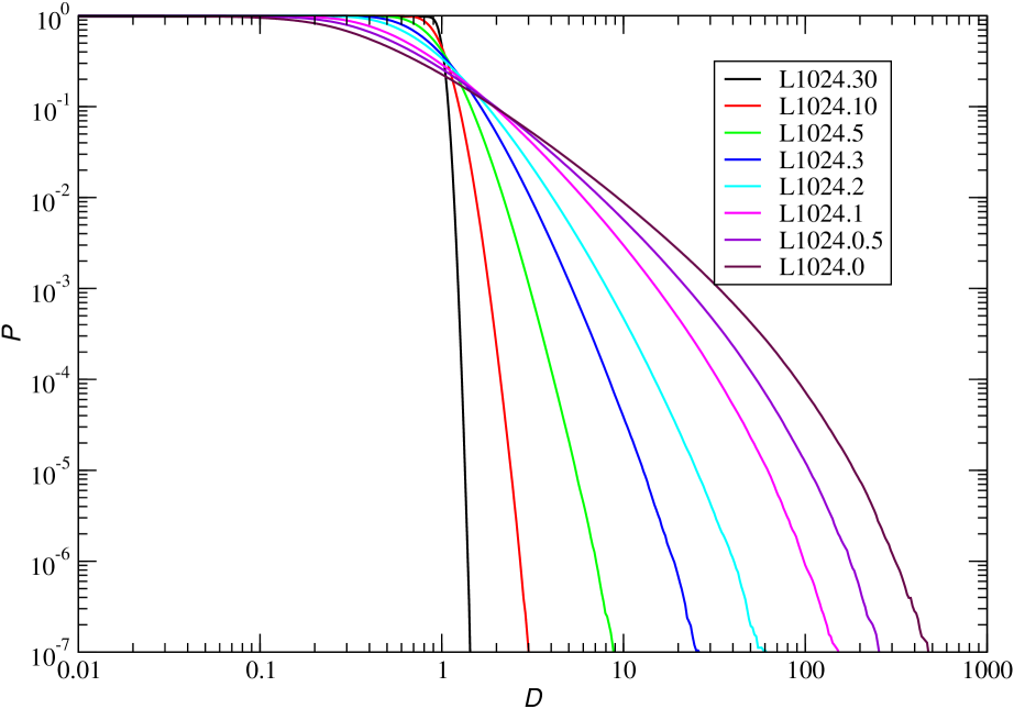
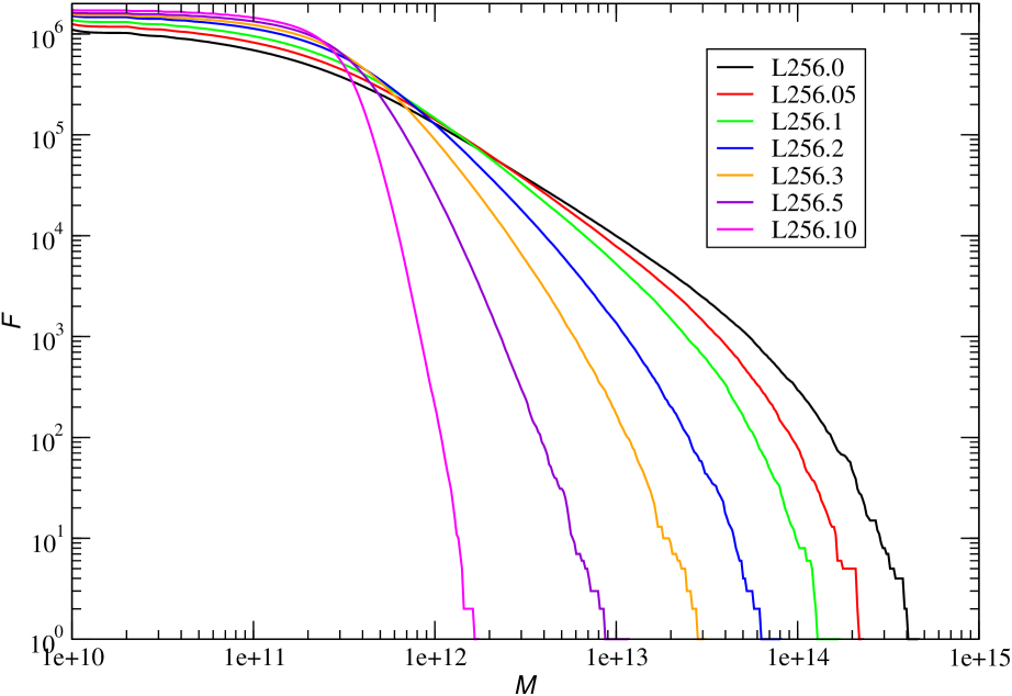
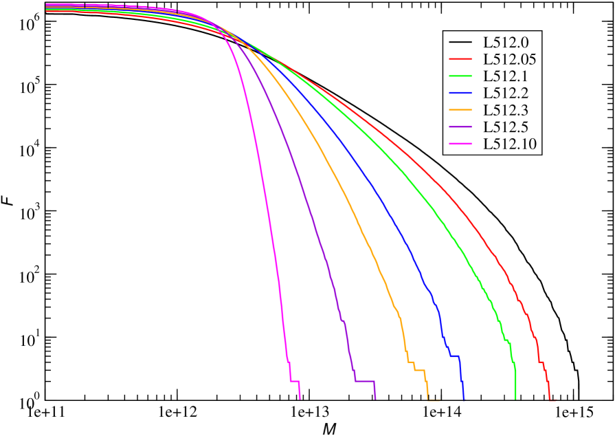
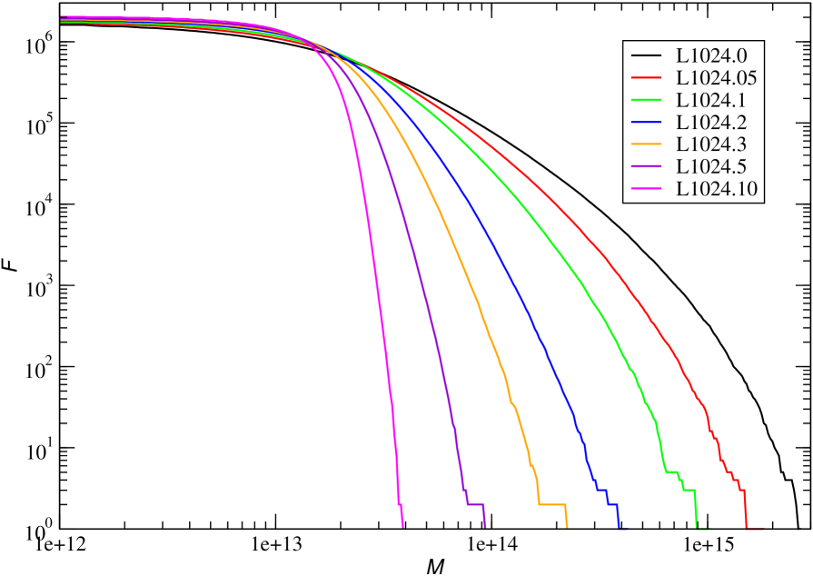
Figure 2: Upper panels: Evolution of cumulative local densities of particles. Middle panels: Evolution of cumulative densities of density fields of models. Lower panels: Evolution of cumulative numbers of model halos. Left, central and right panels are for models L256, L512 and L1024, respectively. In all panels the second index in the model name is redshift.

Traditionally the bias parameter $b$ is defined using density contrasts:

$$b=\delta_{g}/\delta_{m},$$ (3)

where $\delta_{g}$ and $\delta_{m}$ are density contrasts of galaxies and matter. This definition ignores the fact, that in voids the galaxy density is equal to zero, and the galaxy density contrast $\delta_{g}=-1$, which leads to unphysical results. To avoid this difficulty we define the bias through correlation functions of galaxies and matter, following the original definition by Kaiser (1984). Also we consider the bias not as a constant, but as a function of the separation $r$ of galaxies in the correlation function, $b(r)$.

We calculated the correlation functions $\xi(r)$ for all samples of $\Lambda$CDM models with a series of particle density limits. The ratio of correlations functions of samples with particle density limits $\rho_{0}>0$ to limit $\rho_{0}=0$ (which contains all particles) defines the bias function $b(r,\rho_{0})$:

$$b^{2}(r,\rho_{0})=\xi(r,\rho_{0})/\xi(r,0).$$ (4)

Bias depends on the luminosity of galaxies, in our case on the particle density threshold $\rho_{0}$, used in the calculation of correlation functions.

Bias functions have a plateau at $6\leq r\leq 20~{}h^{-1}\,{\rm Mpc}$, see Fig. 5 below. This feature is similar to the plateau around $k\approx 0.03$ $h$ Mpc^-1 of relative power spectra (Einasto et al., 2019). Following Einasto et al. (2020, 2021b) we use this plateau to measure the relative amplitude of the correlation function, i.e. of the bias function, as the bias parameter,

$$b(\rho_{0})=b(r_{0},\rho_{o}),$$ (5)

where $r_{0}$ is the value of the separation $r$ to measure the amplitude of the bias function. We calculated for all samples bias parameters for two values of the comoving separation: $r_{0}=r_{6}=6~{}h^{-1}\,{\rm Mpc}$, and $r_{0}=r_{10}=10~{}h^{-1}\,{\rm Mpc}$, as functions of the particle density limit, $\rho_{0}$. The comoving separation $r_{6}=6~{}h^{-1}\,{\rm Mpc}$ was used by Einasto et al. (2021b) to estimate bias parameters for the present epoch $z=0$. The present analyse suggested that for earlier epochs the value $r_{10}=10~{}h^{-1}\,{\rm Mpc}$ is preferable. At smaller distances, bias functions are influenced by the distribution of particles in halos, and at larger distances, the bias functions have wiggles, which makes difficult the comparison of samples with various particle density limits.

3 Evolution of particle densities and of the density field

In this Section we compare first the evolution of the variance of density perturbations. Thereafter we discuss the evolution of particle densities and density fields with the cosmic epoch $z$, and density distributions of biased model samples. Finally we describe the evolution of density field halos.

3.1 Evolution of the variance of density perturbations with cosmic epoch $z$

We found density fields of models L256, L512 and L1024 for all epochs for which we have computer outputs. Using these fields we calculated the second moment or variance $\sigma^{2}$ of density fields. It is useful to call $\sigma$ as the dispersion of the density field. The evolution of $\sigma$ for various smoothing parameter $R$ values is shown in left panel of Fig. 1. We see that the growth of the density dispersion with cosmic epoch is approximately linear in $\log(\sigma)$ – $\log(1+z)$ diagram for smoothing length $R=8~{}h^{-1}\,{\rm Mpc}$. For smaller smoothing lengths deviations from a linear growth in smaller redshift $z$ region are visible.

It is remarkable that the growth of $\sigma$ of different models but with identical smoothing length $R$ are very close. The dispersion $\sigma_{8}$ found with $R=8~{}h^{-1}\,{\rm Mpc}$ using the $B_{3}$-spline smoothing is given in Table LABEL:Tab1. For all models is is close to value $\sigma_{8}=0.64$. All models were calculated with initial dispersion parameter $\sigma_{8}=0.84$, which corresponds to the linear evolution of density perturbations. As we see, the actual value of $\sigma_{8}$ is slightly lower than the linearly extrapolated value. What is important for the use of our models is the fact, that actual density dispersions of all models for identical smoothing lengths are very close to each other.

Right panel of Fig. 1 presents the dependence of the growth of the dispersion of density fluctuations on smoothing length $R$ and redshift $z$. This dependence is also almost linear in logarithmic scale.

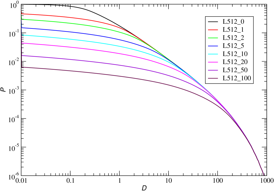
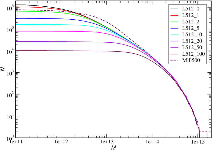
Figure 3: Left: Cumulative density distributions of biased L512 model samples, normalised to the total number of particles. Right: Cumulative numbers of density field halos of biased L512 model samples. Both distributions are given for various particle density limits $\rho_{0}$, indicated as symbol label. For comparison we show by dashed line in the right panel the cumulative distribution of halo mass of the Millennium simulation. All distributions are for the present epoch $z=0$.

3.2 Evolution of particle densities and density fields with cosmic epoch $z$

During the simulations of $\Lambda$CDM models we found for each particle the local density. This local density depends on the resolution of simulation, and has an effective smoothing length $R_{0}=L_{0}/N_{\mathrm{grid}}$ in units $h^{-1}\,{\rm Mpc}$, given in Table  LABEL:Tab1. This local density $\rho_{0}$ was used to select particles to form biased model samples, which correspond to simulated galaxy samples. We show in upper panels of Fig. 2 the evolution of cumulative local densities of particles with cosmic epoch $z$ for our models L256, L512 and L1024, normalised to the total number of particles. This Figure allows to see the range of possible density limits $\rho_{0}$ to select particles for simulated galaxy samples at particular epoch.

For comparison we show in middle panels of Fig. 2 the evolution of density fields with cosmic epoch of the same models. The comparison of upper and middle panels of Fig. 2 shows that distributions of particle densities are different from the distribution of densities of respective density fields – cumulative densities of particles are much higher than cumulative densities of density fields. This difference increases with cosmic epoch (decreasing $z$ value). The reason for these differences lies in the volume occupied by particles in high-density regions, which is much smaller than the fraction of these particles in the total sample of all particles.

Fig. 2 shows also that distributions of particle densities and density fields depend on the model size – upper limits of particle densities and density field values of the model L256 are higher than those of models L512 and L1024. This difference is due to various resolution of models – the effective smoothing length of the model L256 is $0.5~{}h^{-1}\,{\rm Mpc}$, of the model L512 it is $1~{}h^{-1}\,{\rm Mpc}$, and of the model L1024 it is $2~{}h^{-1}\,{\rm Mpc}$, as shown in Table LABEL:Tab1.

Fig.  2 shows that for the simulation L256 we can use particle density limits for biased samples, $\rho_{0}\leq 100$, only for epochs $z\leq 5$, since at epoch $z\geq 5$ there are no particles with $\rho\geq 100$. Thus for this simulation and epoch $z\geq 10$ we can use only particles with density limit $\rho_{0}\leq 10$. The range of possible density limits for simulations L512 and L1024 is smaller.

We show in the left panel of Fig. 3 cumulative densities of particles for biased samples of the simulation L512 for various particle density limit $\rho_{0}$ at the present epoch $z=0$. The upper curve presents the cumulative densities of particles of the whole unbiased model L512.00, following curves show distributions for biased models with particle density limits up to $\rho_{0}=100$. We see that at highest densities all curves coincide, and that curves for biased samples deviate from the unbiased model at densities, approximately equal to the limit $\rho_{0}$.

3.3 Evolution of halos of density fields

In this paper we used particle density limited samples to simulate galaxies. An alternative is to use density field halos. We calculated for all models and simulation epochs density field halos. Usually halos are formed using simulation particles. Another possibility is to use high-resolution density fields. We developed a simple halo finding algorithm, which finds peaks of density fields. Halos are formed by adding densities of surrounding 27 cells, including the central peak cell. This halo finding algorithm is very fast. The cumulative distribution of halos masses of all three models and simulation epochs is shown in bottom panels of Fig. 2. Cumulative halo mass functions of biased L512 models for the present epoch are shown in Fig. 3.

The comparison of upper and lower panels of Fig. 2 shows that cumulative distributions of local densities of particles and halos of various masses have some similarity for all simulation epochs. However, there exist differences, which are largest at low density and halo masse ranges. These difference are due to the fact that our halos do not contain subhalos – halos sum densities within the whole region $\pm 1$ cells around the central peak.

Density field halos can be found also using catalogs of simulated galaxies. To test this possibility we calculated density fields for Millennium simulation (Springel et al., 2005) galaxies by Croton et al. (2006). Fig. 3 shows by dashed line the cumulative distribution of masses of Millennium density field halos. Halos were found using the same procedure as for $\Lambda$CDM model halos. Millennium simulation has the box size $500~{}h^{-1}\,{\rm Mpc}$, very close to out L512 model, thus results are comparable. We see that in high-mass halo region distributions of our L512 model and Millennium simulation coincide. In small mass region our L512 model yields higher number of halos, since it uses all particles.

We see that the use of halos instead of particles can be applied to study the evolution of the bias parameter. However, in this case the whole analysis should be made using halos. The comparison of halo and particles distributions shows, that the use of all particles yields more detailed information on the internal structure of halos. For this reason we use for the detailed analysis only particle density selected biased model samples. As shown by Einasto et al. (2019), particle density limited samples and ordinary halo mass selected samples yield density fields, very similar to density fields of real luminosity limited SDSS samples.

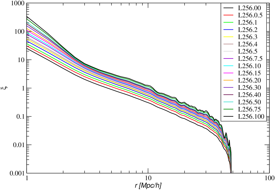
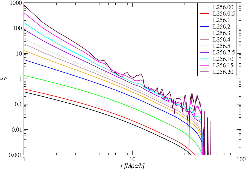
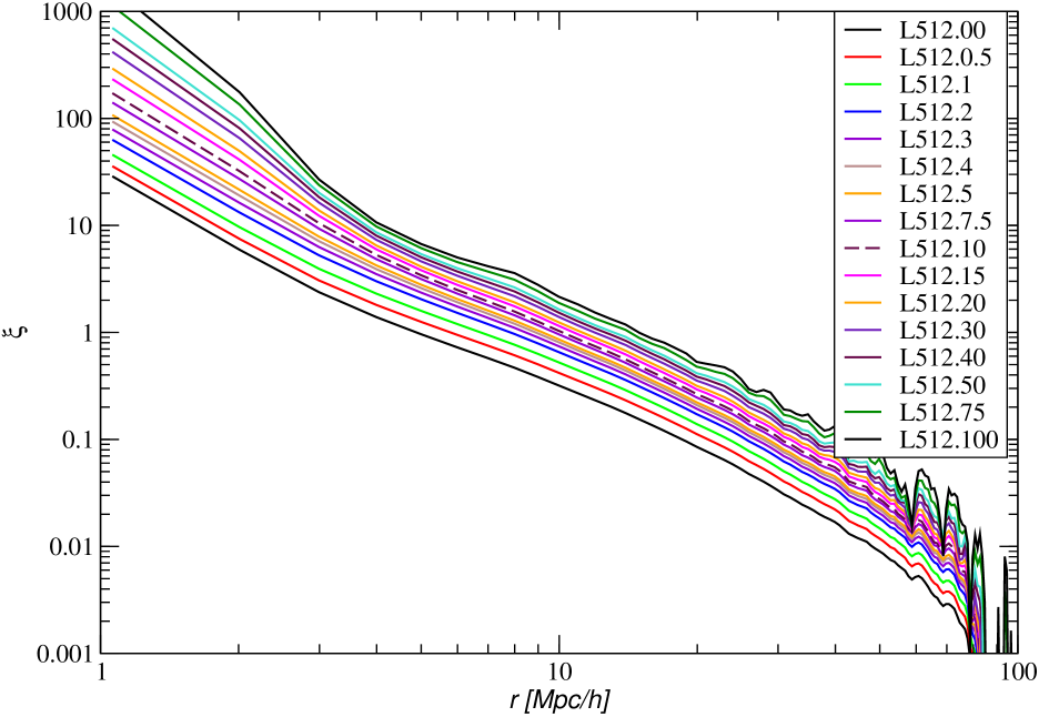
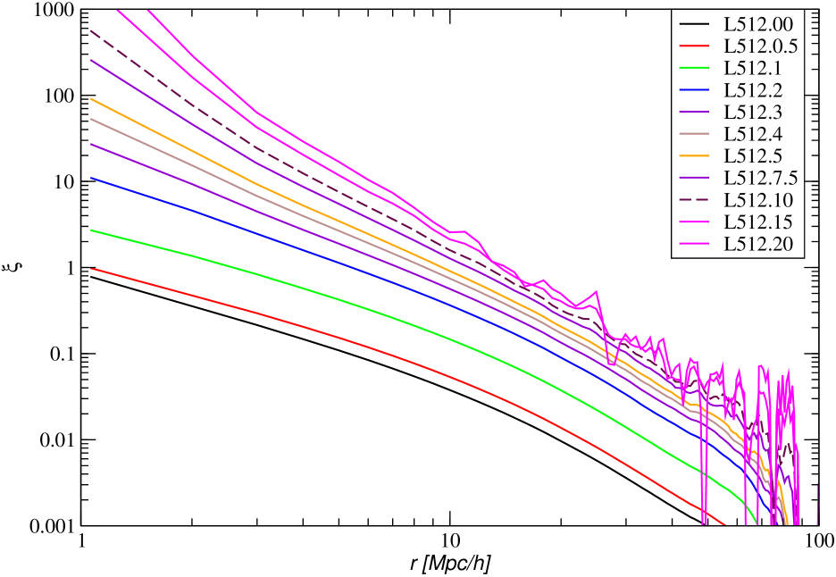
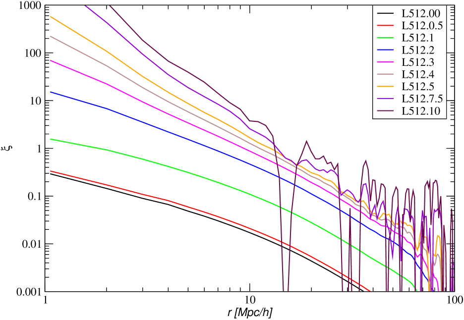
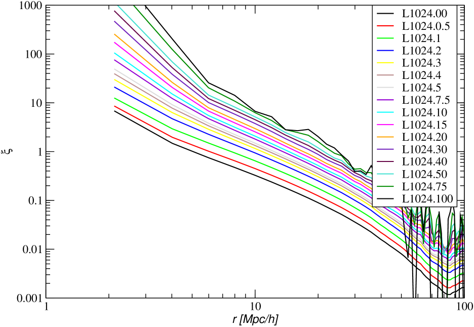
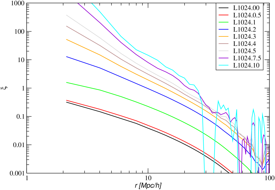
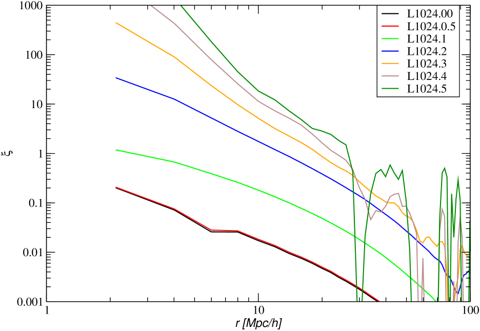
Figure 4: Correlation functions of galaxies, $\xi(r)$ for epochs $z=0,~{}3,~{}5$, shown respectively in the left, central and right panels. Upper panels are for the model L256, middle panels for the model L512, and lower panels for the L1024 model. Density limits $\rho_{0}$ are indicated as symbol labels.

4 Evolution of biasing properties of $\Lambda$CDM models

In this Section we consider the evolution of correlation and bias functions of biased (simulated galaxy) $\Lambda$CDM models. Next we describe the evolution of bias parameters with cosmic epoch. Bias parameters were derived for various particle density limits. In order to get bias parameters for comparable objects we calculated bias parameters for identical fractions of galaxies in samples. The Section ends with the error analysis.

4.1 Evolution of correlation functions of $\Lambda$CDM models

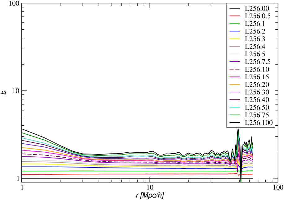
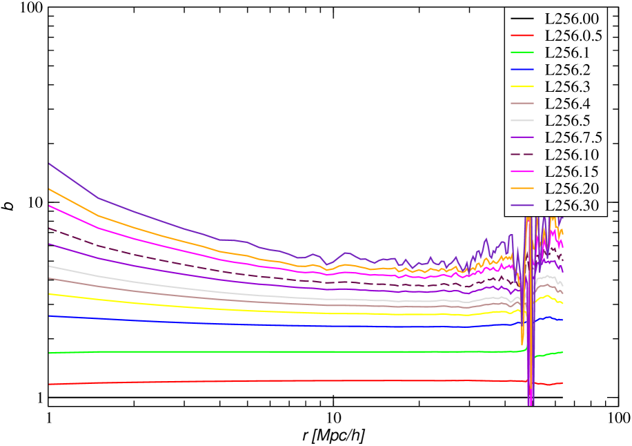
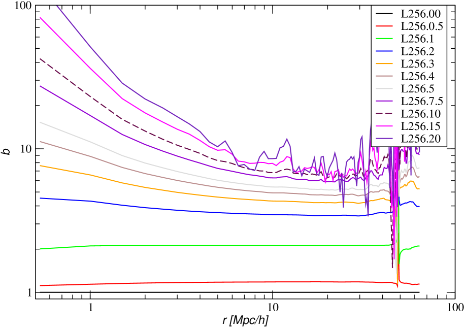
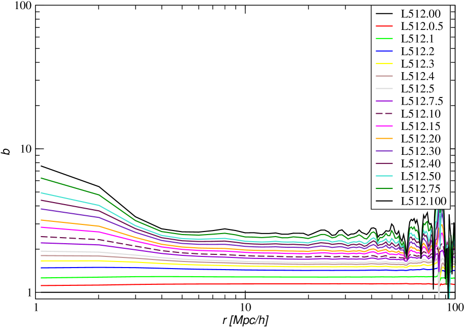
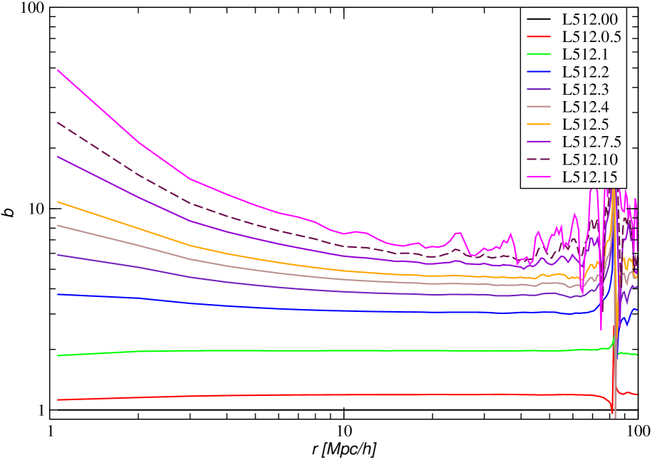
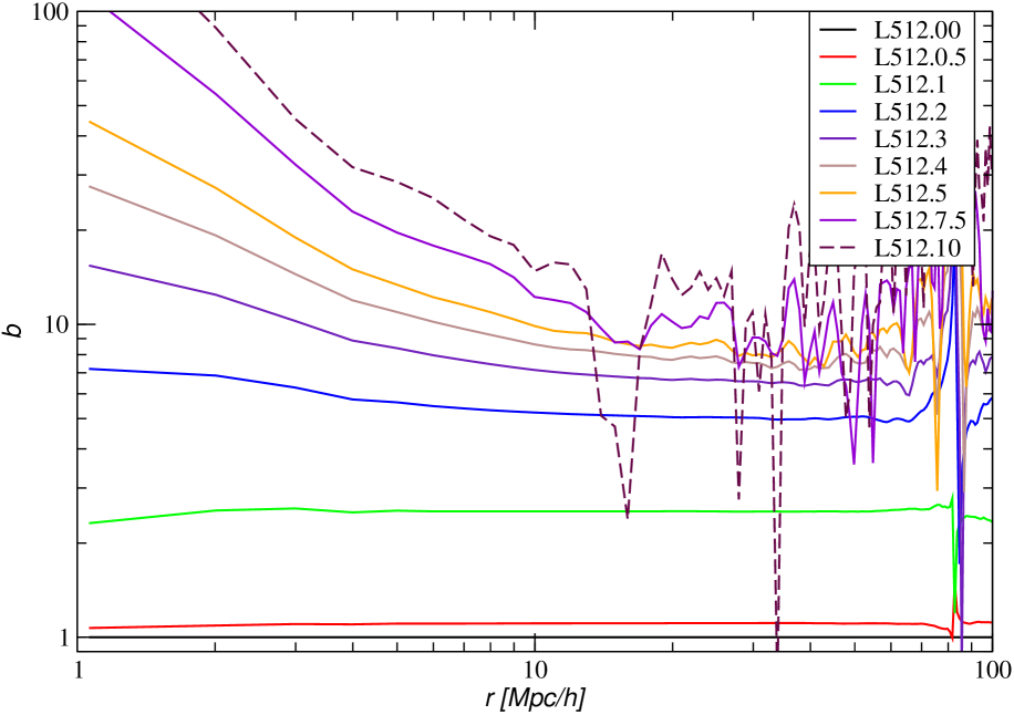
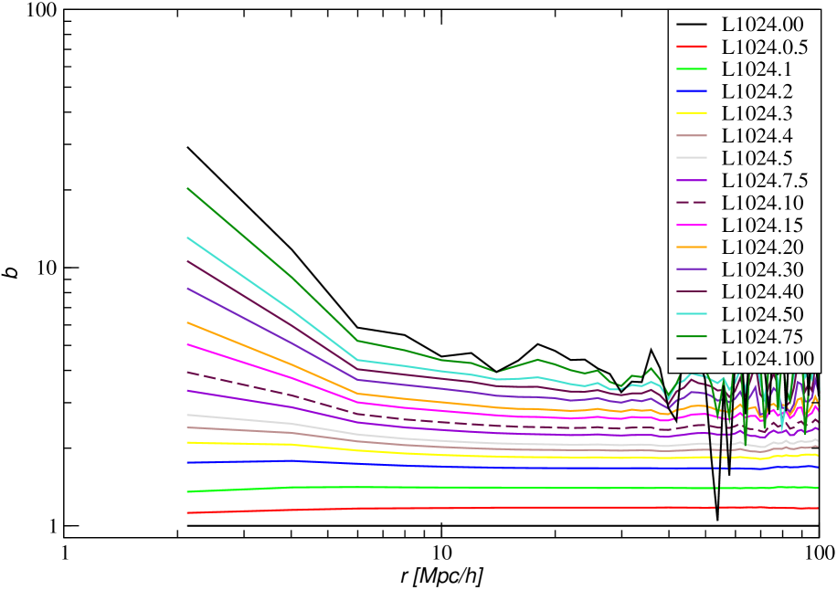
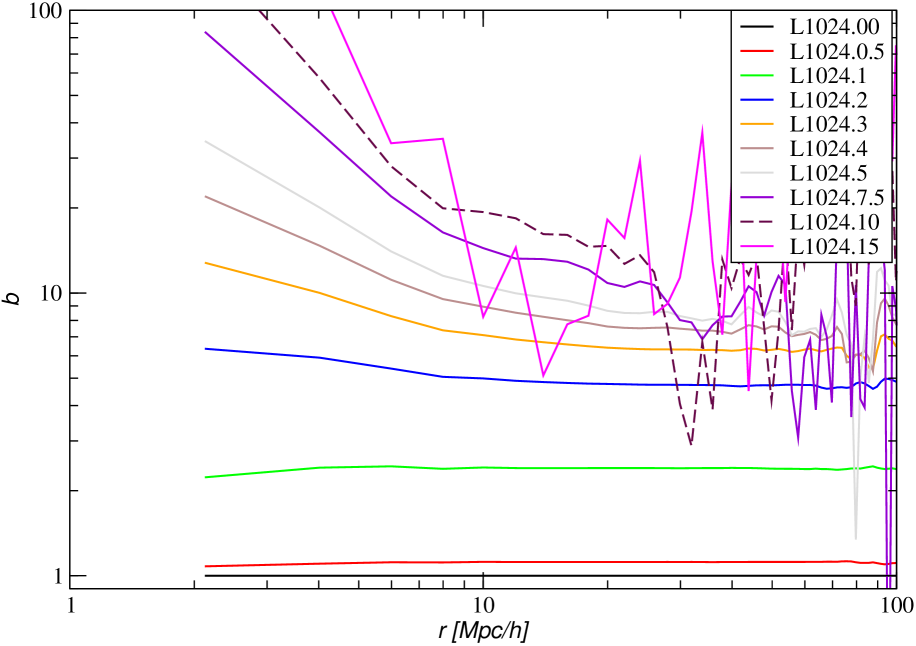
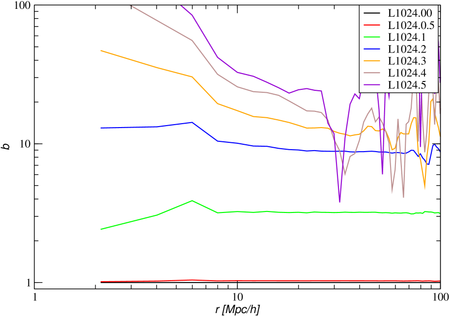
Figure 5: Bias functions, $b(r)$, as functions of the galaxy pair separation $r$ for epochs $z=0,~{}3,~{}5$, shown respectively in the left, central and right panels. Upper panels show bias of the model L256, middle panels of the model L512, and lower panels of the L1024 model. Density limits $\rho_{0}$ are indicated as symbol labels.

We show in Fig. 4 a series of correlation functions for various particle density limits $\rho_{0}$. Left, central and right panels are for epochs $z=0,~{}3,~{}5$, respectively,. Results for L256, L512 and L1024 models are in upper, middle and lower panels, all found with grid resolution $N_{\mathrm{grid}}=1024^{3}$. Here samples with density limit $\rho_{0}=0$ are the samples with all particles and represents the whole DM simulation. On smaller separations $r\leq 5~{}h^{-1}\,{\rm Mpc}$ correlation functions describe the distribution of particles in DM halos, for a discussion of this phenomenon see Einasto et al. (2020). For larger separations correlation functions describe fractal properties of the cosmic web. The fractal dimension function, $D(x)=3+\gamma(r)$, is defined through the logarithmic gradient of the correlation function, $\gamma(r)=d\log g(r)/d\log r$, where $g(r)=1+\xi(r)$, see Einasto et al. (2020).

Central and right panels of Fig. 4 present correlation functions for epochs $z=3,~{}5$ of simulations. The Figure shows that reliable correlation functions can be found for these epochs only in a limited range of particle density limits, $\rho_{0}$ up to $\rho_{0}\approx 30$. This limit is due to the sparsity of particles with density labels above these limits at respective redshifts, see Fig. 2 for the cumulative distribution of local densities of particles.

4.2 Evolution of bias functions of $\Lambda$CDM models

In Fig. 5 we present bias functions, Eq. (4), for epochs $z=0,~{}3,~{}5$. Upper, middle and lower panels present bias functions for simulations L256, L512 and L1024, respectively, found with grid resolution $N_{\mathrm{grid}}=1024^{3}$. As noted above, bias functions have a plateau at $r\geq 6~{}h^{-1}\,{\rm Mpc}$ for the present epoch $z=0$, see Fig. 5. We used this plateau to measure relative amplitudes of the correlation functions, which define bias parameters. In this separation range, bias functions change, therefore the location of the reference point influences our results. Following Einasto et al. (2021b) we used initially the separation $r_{0}=r_{6}=6~{}h^{-1}\,{\rm Mpc}$.

Higher amplitudes of bias functions at small separations are due to the influence of halos. The comparison of panels for different simulations shows that the influence of halos is limited to separation $r\approx 5~{}h^{-1}\,{\rm Mpc}$ for the present epoch $z=0$, and $r\approx 10~{}h^{-1}\,{\rm Mpc}$ for earlier epochs of the L256 simulation. For L512 and L1024 simulations the influence of halos is seen up to higher separations. To avoid the influence of halos we accepted in the final analysis a higher $r_{0}$ value to find bias parameters, $r_{0}=r_{10}=10~{}h^{-1}\,{\rm Mpc}$.

4.3 Evolution of bias parameters with cosmic epoch

Upper panels of Fig. 6 present the evolution of bias parameters with redshift $z$ for models L256, L512 and L1024, found for a series of particle density limits, $\rho_{0}$, shown as model name second index. Here we used grid resolution $N_{\mathrm{grid}}=1024^{3}$ and separation $r_{10}=10~{}h^{-1}\,{\rm Mpc}$. Fig. 5 shows that bias functions for particle density limits $\rho_{0}>5$ have wiggles already at the separation $r\approx 10~{}h^{-1}\,{\rm Mpc}$, used in the determination of bias parameters. These wiggles are due to decreasing number of particles at respective separations, and decrease bias parameter values for early epochs and high particle density limit $\rho_{0}$ of models L512 and L1024. However, in the further analysis with reduced bias parameters we do not use these regions of bias functions.

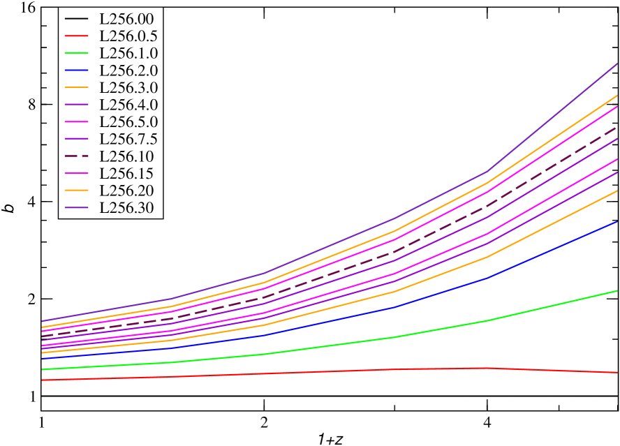
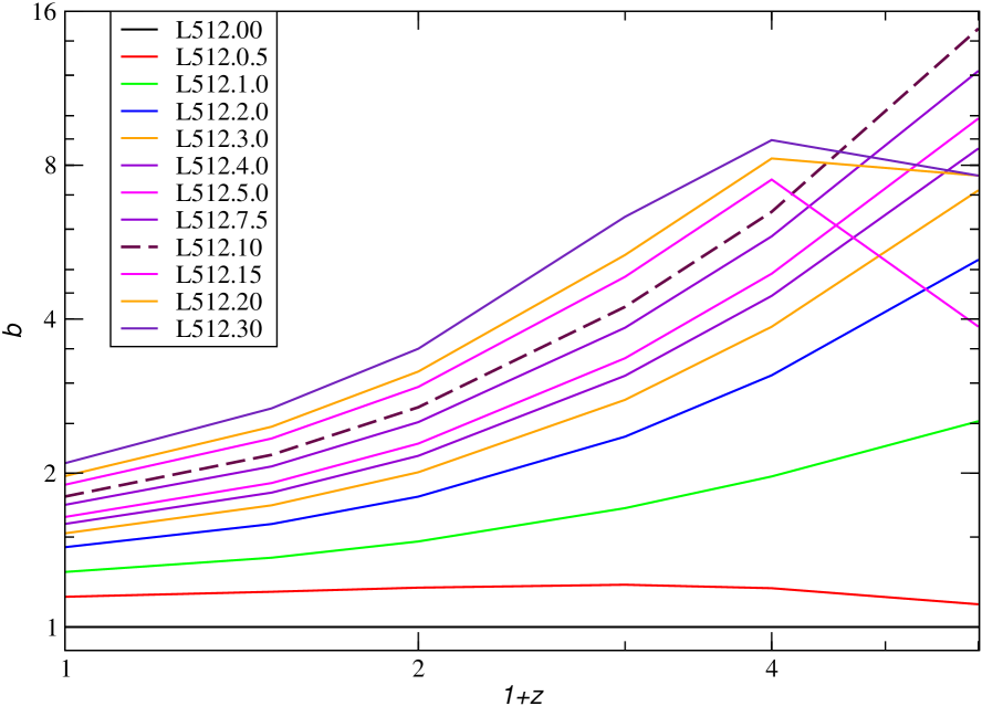
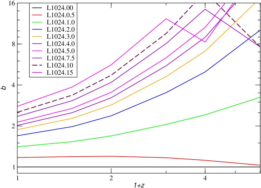
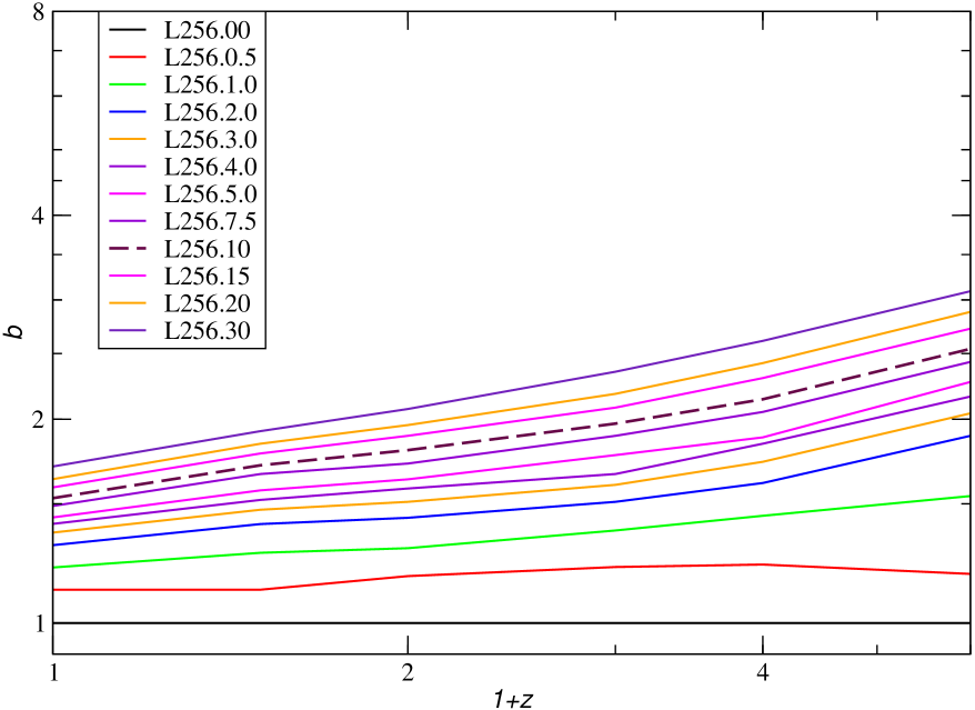
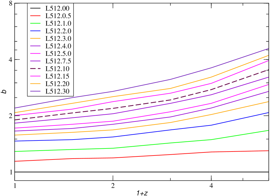
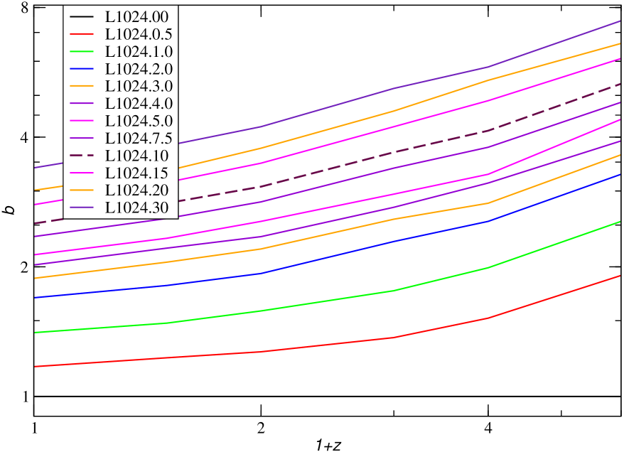
Figure 6: Top: Evolution of bias parameter values with epoch of simulations $z$, using fixed density limits $\rho_{0}$, indicated as symbol labels. Correlation and bias functions were found with resolution $N_{\mathrm{grid}}=1024^{3}$. Bottom: Evolution of bias parameters with epoch of simulations $z$. Bias parameters are calculated for identical fraction of particles, separately for different simulations and epochs. Density limits $\rho_{0}$ are indicated as symbol labels.

Lower panels of Fig.  6 and Tables 2 to 4 present bias parameters as functions of the cosmic epoch $z$, calculated for identical fraction of particles at all simulations and epochs, as described in the next subsection, and using separation $r_{0}=R_{10}=10~{}h^{-1}\,{\rm Mpc}$ to find bias parameters. As expected, the reduced bias parameter values are lower than values, found for fixed particle density levels. The comparison of bias parameters of models L256, L512 and L1024 shows, that bias parameters for models with larger simulation box sizes are higher than in the model of smaller size. We discuss this effect in more detail in the next Section.

Table 2: Bias parameters of L256 particle-density-limited models

Sample	$F(\rho_{0})$	$1/F$	$z=0$	$z=0.5$	$z=1$	$z=2$	$z=3$	$z=5$
(1)	(2)	(3)	(4)	(5)	(6)	(7)	(8)	(9)
L256.00	1.00000	1.0000	1.000	1.000	1.000	1.000	1.000	1.000
L256.05	0.89665	1.1153	1.120	1.147	1.173	1.21	1.220	1.182
L256.1	0.81224	1.2312	1.208	1.27	1.29	1.37	1.44	1.54
L256.2	0.71285	1.4028	1.303	1.40	1.43	1.51	1.61	1.89
L256.3	0.65022	1.5379	1.360	1.47	1.51	1.60	1.73	2.04
L256.4	0.60490	1.6532	1.401	1.52	1.58	1.66	1.84	2.16
L256.5	0.56995	1.7545	1.432	1.57	1.63	1.77	1.88	2.27
L256.7.5	0.50768	1.9697	1.489	1.66	1.72	1.89	2.05	2.43
L256.10	0.46503	2.1504	1.529	1.71	1.80	1.97	2.14	2.54
L256.15	0.40695	2.4573	1.586	1.78	1.89	2.08	2.30	2.72
L256.20	0.36648	2.7287	1.631	1.84	1.96	2.18	2.42	2.88
L256.30	0.30907	3.2355	1.703	1.92	2.07	2.35	2.61	3.09

The columns show the (1) sample name; (2) the fraction of particles $F(\rho_{0})$ at particle-density limit $\rho_{0}$; (3) $1/F(\rho_{0})$: (4) - (9) the bias parameters, calculated for epochs $z=0,~{}0.5,~{}1,~{}2,~{}3,~{}5$.

Table 3: Bias parameters of L512 particle-density-limited models

Sample	$F(\rho_{0})$	$1/F(\rho_{0})$	$z=0$	$z=0.5$	$z=1$	$z=2$	$z=3$	$z=5$
(1)	(2)	(3)	(4)	(5)	(6)	(7)	(8)	(9)
L512.00	1.00000	1.000	1.000	1.00	1.00	1.00	1.00	1.00
L512.0.5	0.89972	1.112	1.141	1.18	1.19	1.24	1.28	1.30
L512.1	0.79682	1.255	1.288	1.32	1.34	1.43	1.49	1.67
L512.2	0.67842	1.474	1.464	1.49	1.54	1.68	1.78	2.08
L512.3	0.60629	1.649	1.576	1.63	1.68	1.84	2.03	2.38
L512.4	0.55536	1.801	1.656	1.71	1.80	1.97	2.20	2.70
L512.5	0.51659	1.936	1.718	1.80	1.87	2.10	2.33	2.94
L512.7.5	0.44900	2.227	1.826	1.95	2.05	2.33	2.59	3.22
L512.10	0.40359	2.478	1.900	2.07	2.19	2.43	2.76	3.53
L512.15	0.34314	2.914	2.006	2.17	2.38	2.64	2.98	3.95
L512.20	0.30235	3.307	2.078	2.33	2.53	2.80	3.22	4.21
L512.30	0.24726	4.044	2.199	2.50	2.70	3.13	3.61	4.58

The columns show the (1) sample name; (2) the fraction of particles $F_{0}$ at particle-density limit $\rho_{0}$; (3) parameter $b_{c}=1/F_{0}$; (4) - (9) the bias parameters, calculated for epochs $z=0,~{}0.5,~{}1,~{}2,~{}3,~{}5$.

Table 4: Bias parameters of L1024 particle-density-limited models

Sample	$F(\rho_{0})$	$1/F(\rho_{0})$	$z=0$	$z=0.5$	$z=1$	$z=2$	$z=3$	$z=5$
(1)	(2)	(3)	(4)	(5)	(6)	(7)	(8)	(9)
L1024.00	1.00000	1.000	1.000	1.00	1.00	1.00	1.00	1.00
L1024.0.5	0.90150	1.109	1.173	1.23	1.27	1.37	1.52	1.91
L1024.1	0.75359	1.327	1.407	1.48	1.58	1.76	1.99	2.55
L1024.2	0.58092	1.721	1.695	1.81	1.93	2.29	2.55	3.28
L1024.3	0.48154	2.077	1.881	2.05	2.20	2.58	2.81	3.64
L1024.4	0.41490	2.410	2.020	2.21	2.35	2.75	3.13	3.92
L1024.5	0.36639	2.729	2.133	2.33	2.55	2.95	3.28	4.40
L1024.7.5	0.28614	3.495	2.351	2.59	2.83	3.39	3.79	4.82
L1024.10	0.23579	4.241	2.521	2.81	3.07	3.69	4.14	5.32
L1024.15	0.16869	5.928	2.788	3.14	3.48	4.23	4.86	6.09
L1024.20	0.13631	7.336	3.010	3.34	3.77	4.60	5.42	6.60
L1024.30	0.09132	10.951	3.394	3.82	4.23	5.19	5.82	7.45

The columns show the (1) sample name; (2) the fraction of particles $F_{0}$ at particle-density limit $\rho_{0}$; (3) parameter $b_{c}=1/F_{0}$; (4) - (9) the bias parameters, calculated for epochs $z=0,~{}0.5,~{}1,~{}2,~{}3,~{}5$.

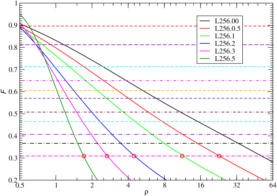
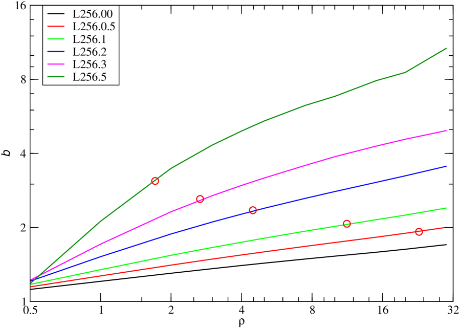
Figure 7: Left: Particle density distribution of model L256 for epochs $z=0,~{}0.5,~{}1,~{}2,~{}3,~{}5,~{}10$. Horisontal lines show cumulative density levels used in calculation of bias values. Right: Bias values for various particle density levels $\rho_{0}$ of the model L256 for the same epochs.

4.4 Reduction of bias parameters to identical fraction of galaxies

In the first stage of our study we used identical particle density limits $\rho_{0}$ to select biased samples of particles for all simulation epochs. However, particle densities evolve with time, and identical particle density limits correspond at different epochs to different objects. To get bias parameters for objects of comparable properties it is needed to bring bias values to a comparable system. To do this we used identical fraction of particles, separately for each model and simulation epoch.

This reduction was made in a two step procedure. First we found the cumulative distribution of the fraction of particles $F(\rho_{0})=N(\rho_{0})/N(0)$ as function of $\rho_{0}$, as done in Fig. 3. Left panel of Fig. 7 shows these distributions for the simulation L256 and epochs $z=0,~{}0.5,~{}1,~{}2,~{}3,~{}5$. Horisontal dashed lines show fraction levels, used in the model L256 at present epoch $z=0$ to select particles for biased sample populations for particle density limits $\rho_{0}=0.5$ to $\rho_{0}=30$. These fractions are given in Table 2 for the L256 simulation, and in Tables 3 and 4 for L512 and L1024 simulations. Using these $F(\rho_{0})$ values we found by interpolation for each evolution epoch $z$ and the fraction $F(\rho_{0})$ the particle density $\rho_{0}$, which at given epoch corresponds to the same population, defined by the respective fraction. For the L256.30 sample and simulation epochs $z=0.5,~{}1.0,~{}2.0,~{}3.0,~{}5.0$ particle density $\rho_{0}$ values, corresponding to $F(\rho_{0})=0.30907$, are shown as red circles.

In the second step we used $\rho_{0}$ values, obtained in the first step at the same fraction of particles $F(\rho_{0})$, to find bias $b$ values for corresponding epochs, using the $b(\rho_{0})$ diagram, shown in the right panel of Fig. 7. Again points in the $b(\rho_{0})$ diagram, corresponding to the L256.30 sample, are shown as red circles. In both panels points corresponding to identical epochs are plotted with curves of identical colour. This interpolation procedure was applied to found reduced bias values for simulations L256, L512 and L1024, given in Tables 2, 3 and 4 by two decimal digits.

This procedure does not take into account the increase of masses of galaxies with time. Actually masses of halos and galaxies increase with time (Chiang et al., 2013). However, this increase is rather modest (Park et al., 2022), and will not change our results considerably, see the Discussion.

4.5 Error analysis

The number of particles in simulations is very high ($512^{3}$), thus random errors of correlation and bias functions are very small, as found by Einasto et al. (2021b). Only at early epochs the number of particles for high $\rho_{0}$ values is small and errors are large, as seen from Figs. 4 and 5. However, these regions of bias function are not used for further analysis with reduced $\rho_{0}$ values. In the $b(\rho_{0})$ diagram in the right panel of Fig. 7 red coloured points are for samples with particle density limit $\rho_{0}=30$. All points for samples with lower particle density limit are situated at lower reduced $\rho_{0}$ levels, where random errors are small. Thus essential errors of our analysis are systematic differences, due to variable simulation bos sizes and respective resolutions in calculation of correlation functions.

Basic data for our analysis are particle samples and density fields, determined by the distribution of particles. To check our simulations for possible errors we analysed in Section 3 density fields of simulations for various box sizes, $L_{0}$, smoothing scales $R$, and simulation epochs $z$. Results of this analyse are shown in Fig. 1. We see that the dispersion $\sigma$ varies with box size $L_{0}$, smoothing scale $R$, and simulation epoch $z$ as expected. Thus variations in these parameters yield simulations with good internal consistency. Thus the influence of largest modes of density perturbations is small.

Essential results of our analysis are presented in Tables 2 – 4, and in lower panels of Fig. 6. This Figure shows, first of all, that bias curves for increasing particle density selection level $\rho_{0}$ form very regular sequences. This suggests that errors in reducing bias parameters to identical fractions of particles cannot be large. However, there exist differences in bias parameters, as found for different box sizes – at all evolutionary epochs $b$ values for larger box sizes are larger. These differences characterise the possible range of uncertainty in bias parameters. We discuss this effect in more detail in the next Section.

5 Discussion

Here we compare our data with results by other studies. Thereafter we discuss the influence of a low-density homogeneous population in voids. The Section ends with the discussion of our results for the bias parameter.

5.1 Comparison with earlier studies

We begin the comparison with the analysis by Fry & Gaztanaga (1994), who derived galaxy correlation functions of samples of increasing depth, using CfA, Southern Sky Redshift Survey (SSRS) and IRAS redshift catalogs. Authors found that the correlation length $r$ of CfA samples increases with sample depth, $z_{lim}=5000$ km/s to $z_{lim}=9000$ km/s, from $r=3.7~{}h^{-1}\,{\rm Mpc}$ to $r=5.8~{}h^{-1}\,{\rm Mpc}$ in real space, and from $r=4.5~{}h^{-1}\,{\rm Mpc}$ to $r=6.8~{}h^{-1}\,{\rm Mpc}$ in redshift space. A similar growth is observed in SSRS and IRAS samples. These data confirm results by Einasto et al. (1986), Einasto & Einasto (1989) and Einasto et al. (1989) and Einasto et al. (1994), who explained this increase as the approach to a representative sample of the universe with increasing fraction of void volumes in samples, see the next subsection.

Fry (1996) investigated th evolution of bias, using a model in which galaxies are formed at a fixed time and follow motions, determined by the gravitational potential. The bias parameter decreases from $b=2.5$ at expansion factor $a=2$ to $b=1.15$ at $a=20$. Fry concluded that bias must have been larger in the past.

Tegmark & Peebles (1998) investigated the time evolution of bias using perturbation theory, and adopting a time dependent galaxy formation model. Result for the bias parameter depend on the galaxy formation model. Between redshifts $z=5$ and $z=0$ the bias parameter decreases in most models from $b\approx 2.5$ to $b\approx 1.2$. For all models in a far future the bias parameter approaches to unity.

Now we compare our results with observational data on bias values for high-redshift objects. Adelberger et al. (1998) estimated correlation functions for Lyman-break galaxies at redshift $z\sim 3$. Comparison with models depends on cosmological parameters accepted, for $\Omega_{m}=0.3$ and flat cosmogony authors obtained $b=4.0\pm 0.7$. This value is similar to our data for high luminosity (high particle threshold limit $\rho_{0}$) samples.

Song et al. (2021) used Dark Energy Spectroscopy Instrument to study galaxy clustering at redshift up to $z=1.6$ in several redshift slices. Authors found that with increasing redshift from $z=0.5$ to $z=1.1$ the linear bias parameter of Luminous Red Galaxies increases from $b_{1}=2.22$ to $b_{1}=2.94$, and from $b_{1}=1.10$ to $b_{1}=1.45$ for Emission Line Galaxies.

A study by Miyatake et al. (2022) used CMB lensing signals of 1.5 million galaxies at $z\sim 4$ to estimate $\sigma_{8}$ and bias $b$ parameters. Result are given in their Fig. 2 as cosmological constraints for these parameters. For $\Omega_{m}=0.3$ the lensing+clustering constraint suggests $\sigma_{8}(z=0)=0.5$ in good agreement with our calculation, presented in Table LABEL:Tab1. For this $\sigma_{8}$ authors found bias parameter $b\approx 6$, similar to our samples with high particle density limit $\rho_{0}$.

Park et al. (2022) investigated the formation and morphology of the first galaxies in the cosmic morning, $10\geq z\geq 4$, using Horizon Run cosmological simulations with gravity, hydrodynamics and various astrophysics. Among other results authors calculated correlation functions of simulated galaxies in redshift range $z=5-7$, see Fig. 11 by Park et al. (2022). Using data given in this Figure we found bias parameter values $b=10,~{}7,~{}6$ for redshifts $z=7,~{}6,~{}5$, respectively. These data by Park et al. (2022) were found for simulated galaxies with stellar masses $M_{\star}\geq 2\times 10^{9}~{}M_{\odot}$. Our Tables 2 – 4 suggest that these bias values are approximately equivalent to bias of our samples with particle density limit $\rho_{0}\approx 30$.

5.2 Two populations of matter

Differences in the distribution of matter and galaxies were noticed already in the early stage of the study of cosmic web. Quantitatively these differences can be described by differences of correlation lengths in regions containing various amounts of voids in galaxy and simulation samples. In the present study we use $\Lambda$CDM simulations and a wide range of cosmic epochs, starting from $z=30$, and characterise biasing properties by the amplitude of the bias functions – ratios of correlation functions of galaxies and matter. We use samples of particles with various local densities, which characterise objects of different nature. As suggested by White & Rees (1978) and Zeldovich et al. (1982) and confirmed by hydrodynamical models by Cen & Ostriker (1992, 2000), galaxies form only in DM halos and not in under-dense regions in voids. Thus the matter is divided into two components, the clustered matter in galaxies and clusters of galaxies, containing DM and visible galaxies, and the unclustered matter in low density regions, consisting of DM and rarefied baryonic gas, but no stars.

These two populations have very different spatial distribution. The clustered population with galaxies occupies small isolated regions, the rest of the volume in voids is much larger, about 95% of the whole volume of the SDSS sample, for details see Fig. 2 and discussion in Einasto et al. (2018). The amplitude of the relative correlation function, measured by the bias parameter $b$, is sensitive to the fraction of matter in the clustered population and in the unclustered matter in voids, for a discussion see the next Subsection.

Due to differences in spatial distribution, clustered and unclustered populations have different influence to the biasing parameter $b$. The unclustered matter in low density regions rises the bias parameter from $b=1$ for the whole matter to $b\approx 1.5$ at the present epoch, which corresponds to particle density limit $\rho_{0}\approx 3$. As shown by Einasto et al. (2019), this limit separates the unclustered and clustered populations at the level of faintest galaxies. Further increase of bias parameter is due to the inclusion to the sample brighter galaxies.

5.3 The influence of a homogeneous population

The dependence of the bias parameter on the fraction of particles in the clustered population was suggested by Saar (1983), and studied in more detail by Einasto et al. (1986), Einasto & Saar (1987), Gramann & Einasto (1992), Einasto et al. (1994) and Einasto et al. (1999). This factor is crucial to understand our results, thus we give here two simple toy models to explain the idea.

The natural estimator to determine the two-point spatial correlation function is

$$1+\xi(r)={DD(r)\over RR(r)},$$ (6)

where $DD(r)$ and $RR(r)$ are normalised counts of galaxy-galaxy and random-random pairs at separation $r$. Consider a volume of size $V_{0}$, containing galaxies and systems of galaxies like supercluster central regions. Denote counts of galaxy-galaxy and random-random pairs as $DD_{0}(r)$ and $RR_{0}(r)$. Now surround this volume with empty space with no galaxies, and denote the total volume of this sample as $V_{1}$. Galaxy-galaxy counts in the new volume are identical to counts in the original volume, $DD_{1}(r)=DD_{0}(r)$. Random-random counts at separation $r$, $RR_{1}(r)$ are, however lower, since the random sample is diluted over a larger volume $V_{1}$. This rises the amplitude of the correlation function $1+\xi(r)$, the rise is proportional to the ratio of volumes, $V_{0}/V_{1}$. To illustrate this effect we calculated correlation functions for two samples, one for a sample with galaxies of size $100~{}h^{-1}\,{\rm Mpc}$, and the other where this sample is located in a cube of size $200~{}h^{-1}\,{\rm Mpc}$, containing outside the inner cube no galaxies. The bias function is given by the ratio of correlation functions of both samples, $1+\xi(r)=RR_{0}(r)/RR_{1}(r)$. This bias function is shown in Fig. 8. As we see, over most of the $r$ range it is proportional to square root of the ratio of volumes, $V_{1}/V_{0}$.

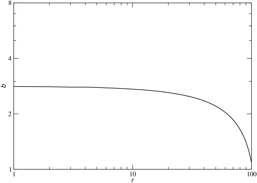
Figure 8: Bias function, found from the ratio of correlation functions $1+\xi(r)=RR_{0}(r)/RR_{1}(r)$.

The second model was suggested by Einasto et al. (1999), we give here a summary of the discussion.

Consider an idealized density field, which consists of a fluctuating clustered component and a background of constant density, so that

$$D_{m}({\bf x})=D_{g}({\bf x})+D_{s}({\bf x});$$ (7)

here subscript $m$ is for all matter, $g$ is for galaxies (the clustered component), and $s$ for the smooth component. The density contrast of the matter is

$$\delta_{m}={D_{m}-\overline{D}_{m}\over\overline{D}_{m}};$$ (8)

or, applying (7),

$$\delta_{m}={D_{g}+D_{s}-(\overline{D}_{g}+\overline{D}_{s})\over\overline{D}_{g}+\overline{D}_{s}}.$$ (9)

Since $D_{s}=\overline{D}_{s}$, we get

$$\delta_{m}={D_{g}-\overline{D}_{g}\over\overline{D}_{m}}=\delta_{g}{\overline{D}_{g}\over\overline{D}_{m}}.$$ (10)

In the last equation $\overline{D}_{g}/\overline{D}_{m}$ is the fraction of matter in the clustered population, $F_{c}$; and we get

$$\delta_{m}=\delta_{g}F_{c}.$$ (11)

According to traditional definition, Eq. (3), $\delta_{g}/\delta_{m}=b$, and we get for the bias factor

$$b={1\over F_{c}}.$$ (12)

Equations (11) and (12) show that the subtraction of a homogeneous population from the whole matter population increases the amplitude of the correlation function (power spectrum) of the remaining clustered population. In this approximation biasing is linear and does not depend on scale. These equations have a simple interpretation. If we subtract from the density field a constant density background but otherwise preserve density fluctuations, then amplitudes of absolute density fluctuations remain the same, but amplitudes of relative fluctuations with respect to the mean density increase by a factor which is determined by the ratio of mean densities.

Calculations made in the present analysis show that the approximate equation (12) is valid for low particle density threshold $\rho_{0}\leq 1$. For larger $\rho_{0}$ values equation (12) predicts too high values for the bias parameter $b$. The reason for this deviation is the difference of the density distribution in voids, which cannot be considered as constant, as assumed in the Eq.  (12).

In this way we see that the amplitude of the correlation function measures the emptiness of samples of galaxies, quantified by the fraction of particles in voids and in the clustered population.

To check how accurately the relation (12) helds we calculated ratios $1/F_{c}$ for the present epoch $z=0$ for all $\rho_{0}$ values, results are given in Tables 2 to 4. We see that in all simulations bias parameter values for particle density threshold $\rho_{0}\leq 3$ are rather close to values, found from the relation (12). This is expected, since bias functions $b(r)$ are almost constant for $\rho_{0}\leq 3$, see Fig. 5, i.e. correlation functions have a similar shape and differ only by the amplitude, which defines the bias parameter. For higher $\rho_{0}$ values differences in shapes of correlation functions influence amplitudes of bias functions, and the relation (12) is not valid.

5.4 Evolution of the bias parameter

Basic results of our study are presented in Tables 2, 3 and 4, and in Figs. 5 and 6. The essential impression from Fig. 5 is that bias is not a constant, as assumed in the classical theory (see Eq. (3)), but a function of the separation, $b(r)$. The function has two regions – at small separations it describes the distribution of particles (galaxies) in halos, at large separations it describes the spatial distribution of halos (systems of galaxies). The transition between these regions is determined by the scale of halos (groups and clusters of galaxies), which depends on the evolutionary epoch. Halos are essentially virialised systems with approximately constant physical sizes. Our calculations are done in comoving coordinates, thus in comoving coordinates halos were larger in the past, as shown independently by Chiang et al. (2013)

Fig.  5 demonstrates that for all cosmic epochs bias functions $b(r)$ form regular sequences, depending on galaxy luminosity (particle density limit $\rho_{0}$). With increasing $\rho_{0}$ bias functions $b(r,\rho_{0})$ increase. This is the dependence, first described by Kaiser (1984). Now we have this relationship for a large range of cosmic epochs $z$.

On scales not influenced by halos bias functions have approximately constant amplitudes, which define bias parameters. Fig. 6 shows that bias parameter values $b(z)$ as functions of the cosmic epoch, $b(z)$. Our data show that the bias parameter $b$ was higher in earlier cosmic epochs. In this way our analysis confirms earlier results, discussed above, but in a larger range of evolutionary epochs of the universe. Physical reason for the increase of $b$ with epoch $z$ is simple – in earlier epochs the fraction of matter in voids was larger. During the evolution diffuse matter (DM and rarefied baryonic gas) flows out of voids, as shown among others by Courtois et al. (2017) and Rizzi et al. (2017).

Data presented in lower panels of Fig.  6 show that bias parameter $b$ values for different particle density thresholds $\rho_{0}$ depend on simulation box sizes: bias parameters $b$ are highest for the simulation L1024, and lowest for the L256 simulation. The reason for the dependence on simulation box size is not clear. In all cases correlation functions were calculated using particles without additional smoothing, and bias parameters were reduced to identical fractions of particles in the clustered population.

As discussed above, low $\rho_{0}$ levels correspond to particles in low-density regions and voids. The particle density threshold $\rho_{0}$ level which corresponds to faintest galaxies is known only approximately. A better defined limit is the one, corresponding to $L_{\star}$ and Luminous Red Giant galaxies. As shown by Einasto et al. (2019) for the L512 simulation and the present epoch, $L\geq L_{\star}$ galaxies have the same spatial distribution than DM particles with density threshold $\rho_{0}\geq 10$ in mean density units, see Fig. 10 by Einasto et al. (2019). Correlation and bias functions for this level are drawn in Figs. 5 and 6 with dashed lines.

As shown in 6 and given in Tables 2, 3 and 4, reduced bias parameters $b(10)$ are different in simulations of various size. To find connections for L256 and L1024 simulations, a similar approach can be applied, but this is outside the scope of the present study.

One reason for differences in bias parameters for different epochs is the constant level of the fraction of particles in high-density regions, used in the determination of the bias parameter. Actually groups and clusters of galaxies grow with time by merging and infall of gas and dark matter via filaments, which causes changes of fractions of particles in high-density regions. To reduce our data to similar populations of galaxy systems, we should take into account the growth of systems. However, as shown by Park et al. (2022), the growth of masses (luminosities) of galaxies has little effect on the biasing parameter.

To conclude the discussion, we emphasise the role of different populations in shaping bias functions and parameters. The unclustered matter, consisting of DM particles and diffuse baryonic matter, and filling about 95% of the volume of the universe, is responsible in forming bias functions and parameters up to particle threshold levels $\rho_{0}\leq 3$. Beyond this limit, $\rho_{0}>3$, particle density limited samples of DM simulations represent luminosity limited samples of galaxies of various luminosity. This is the region initially discussed by Kaiser (1984), and recently studied by Norberg et al. (2001), Lahav et al. (2002), Verde et al. (2002), Tegmark et al. (2004) and Zehavi et al. (2011). These studies describe well the relative dependence of the bias parameter on the luminosity, in good agreement with relative dependence of the bias parameter in our DM simulations. However, these studies were not able to reduce bias parameters of galaxies to that of the matter. The reason for this difference could be the insensitivity of methods, applied to find bias parameters, to the smoothly distributed background of unclustered matter. In contrast, the study by Park et al. (2022) allowed to take into account both populations, and to find bias parameters of simulated galaxies in respect to matter.

6 Conclusions

In this paper we studied the evolution of the bias parameter using numerical simulations of the evolution of the cosmic web. Our study is based on three assumptions: (i) – the $\Lambda$CDM model represents real universe; (ii) – particle density selected samples represent galaxy samples; and (iii) – sharp density threshold limit $\rho_{0}$ allows to select biased galaxy (particle) samples. The novelty of our approach lies in the use of numerical simulations in a large range of evolutionary epochs, which allowed to take into account the influence of both populations – the smoothly distributed unclustered matter with no visible galaxies, and the clustered matter with visible galaxies. We used several $\Lambda$CDM simulations and a wide range of evolution epochs and particle density threshold levels to find bias properties in a large range of cosmological parameter space.

Our basic results can be summarised as follows.

1. Bias is a function of particle separation $r$ and particle density selection level $\rho_{0}$, $b(r,\rho_{0})$. On small separations, $r\leq 10~{}h^{-1}\,{\rm Mpc}$, correlation and bias functions describe the distribution of particles (galaxies) in halos (clusters), on larger separations the distribution of halos (clusters).

2. For all cosmic epochs the bias parameter depends on two factors: the fraction of matter in the clustered population, and the particle density (galaxy luminosity) limit of samples. Gravity cannot evacuate voids completely, thus there is always some unclustered matter in voids, and the bias parameter of galaxies is always greater than unity, over the whole range of evolution epochs.

3. For all cosmic epochs bias parameter values form regular sequences, depending on galaxy luminosity (particle density limit), and decreasing with time.

The present study allowed to find bias parameters in a much wider parameter space in time and galaxy luminosity than made in earlier studies. However, we consider the bias parameter for characteristic luminosity $L_{\star}$ as a preliminary one, since simulations in cubes of different size, L256 and L1024, give different results, $b_{\star}=1.5$ and $b_{\star}=2.5$, respectively. Do find a better value of the characteristic bias parameter for the present epoch, $b_{\star}$, and its evolution, a study is needed, which uses simulated galaxies at various epochs.

References

- Adelberger et al. (1998) Adelberger K. L., Steidel C. C., Giavalisco M., Dickinson M., Pettini M., Kellogg M., 1998, ApJ, 505, 18
- Bertschinger (1995) Bertschinger E., 1995, ArXiv:astro-ph/9506070,
- Cen & Ostriker (1992) Cen R., Ostriker J. P., 1992, ApJL, 399, L113
- Cen & Ostriker (2000) Cen R., Ostriker J. P., 2000, ApJ, 538, 83
- Chiang et al. (2013) Chiang Y.-K., Overzier R., Gebhardt K., 2013, ApJ, 779, 127
- Courtois et al. (2017) Courtois H. M., Tully R. B., Hoffman Y., Pomarède D., Graziani R., Dupuy A., 2017, ApJL, 847, L6
- Croton et al. (2006) Croton D. J., et al., 2006, MNRAS, 365, 11
- Dekel (1998) Dekel A., 1998, in Colombi S., Mellier Y., Raban B., eds, Vol. 14, Wide Field Surveys in Cosmology. p. 47 (arXiv:astro-ph/9809291)
- Dekel & Lahav (1999) Dekel A., Lahav O., 1999, ApJ, 520, 24
- Desjacques et al. (2018) Desjacques V., Jeong D., Schmidt F., 2018, Phys. Rep., 733, 1
- Doroshkevich et al. (1980) Doroshkevich A. G., Kotok E. V., Poliudov A. N., Shandarin S. F., Sigov I. S., Novikov I. D., 1980, MNRAS, 192, 321
- Doroshkevich et al. (1982) Doroshkevich A. G., Shandarin S. F., Zeldovich I. B., 1982, Comments on Astrophysics, 9, 265
- Dubois et al. (2021) Dubois Y., et al., 2021, A&A, 651, A109
- Einasto & Einasto (1989) Einasto M., Einasto J., 1989, Tartu Astr. Obs. Teated, 95, 21
- Einasto & Saar (1987) Einasto J., Saar E., 1987, in Hewitt A., Burbidge G., Fang L. Z., eds, IAU Symposium Vol. 124, Observational Cosmology. pp 349–358
- Einasto et al. (1986) Einasto J., Saar E., Klypin A. A., 1986, MNRAS, 219, 457
- Einasto et al. (1989) Einasto J., Einasto M., Gramann M., 1989, MNRAS, 238, 155
- Einasto et al. (1991) Einasto J., Einasto M., Gramann M., Saar E., 1991, MNRAS, 248, 593
- Einasto et al. (1994) Einasto J., Saar E., Einasto M., Freudling W., Gramann M., 1994, ApJ, 429, 465
- Einasto et al. (1999) Einasto J., Einasto M., Tago E., Müller V., Knebe A., Cen R., Starobinsky A. A., Atrio-Barandela F., 1999, ApJ, 519, 456
- Einasto et al. (2018) Einasto J., Suhhonenko I., Liivamägi L. J., Einasto M., 2018, A&A, 616, A141
- Einasto et al. (2019) Einasto J., Liivamägi L. J., Suhhonenko I., Einasto M., 2019, A&A, 630, A62
- Einasto et al. (2020) Einasto J., Hütsi G., Kuutma T., Einasto M., 2020, A&A, 640, A47
- Einasto et al. (2021a) Einasto J., Klypin A., Hütsi G., Liivamägi L.-J., Einasto M., 2021a, A&A, 652, A94
- Einasto et al. (2021b) Einasto J., Hütsi G., Einasto M., 2021b, A&A, 652, A152
- Fry (1996) Fry J. N., 1996, ApJL, 461, L65
- Fry & Gaztanaga (1994) Fry J. N., Gaztanaga E., 1994, ApJ, 425, 1
- Gramann & Einasto (1992) Gramann M., Einasto J., 1992, MNRAS, 254, 453
- Jõeveer & Einasto (1978) Jõeveer M., Einasto J., 1978, in Longair M. S., Einasto J., eds, IAU Symposium Vol. 79, Large Scale Structures in the Universe. pp 241–250
- Jõeveer et al. (1978) Jõeveer M., Einasto J., Tago E., 1978, MNRAS, 185, 357
- Jensen & Szalay (1986) Jensen L. G., Szalay A. S., 1986, ApJL, 305, L5
- Kaiser (1984) Kaiser N., 1984, ApJL, 284, L9
- Lahav et al. (2002) Lahav O., et al., 2002, MNRAS, 333, 961
- Landy & Szalay (1993) Landy S. D., Szalay A. S., 1993, ApJ, 412, 64
- Little & Weinberg (1994) Little B., Weinberg D. H., 1994, MNRAS, 267, 605
- Martínez & Saar (2002) Martínez V. J., Saar E., 2002, Statistics of the Galaxy Distribution. Chapman & Hall/CRC
- Miyatake et al. (2022) Miyatake H., et al., 2022, Phys. Rev. Lett., 129, 061301
- Norberg et al. (2001) Norberg P., et al., 2001, MNRAS, 328, 64
- Park et al. (2022) Park C., et al., 2022, arXiv e-prints, p. arXiv:2202.11925
- Repp & Szapudi (2019a) Repp A., Szapudi I., 2019a, arXiv e-prints, p. arXiv:1904.05048
- Repp & Szapudi (2019b) Repp A., Szapudi I., 2019b, arXiv e-prints, p. arXiv:1912.05557
- Repp & Szapudi (2020a) Repp A., Szapudi I., 2020a, MNRAS, 493, 3449
- Repp & Szapudi (2020b) Repp A., Szapudi I., 2020b, MNRAS, 498, L125
- Rizzi et al. (2017) Rizzi L., Tully R. B., Shaya E. J., Kourkchi E., Karachentsev I. D., 2017, ApJ, 835, 78
- Saar (1983) Saar E., 1983, (private communication)
- Song et al. (2021) Song Y.-S., Zheng Y., Taruya A., 2021, Phys. Rev. D, 104, 043528
- Springel (2005) Springel V., 2005, MNRAS, 364, 1105
- Springel et al. (2005) Springel V., et al., 2005, Nature, 435, 629
- Szapudi & Szalay (1993) Szapudi I., Szalay A. S., 1993, ApJ, 414, 493
- Szapudi et al. (2001) Szapudi I., Prunet S., Pogosyan D., Szalay A. S., Bond J. R., 2001, ApJL, 548, L115
- Szapudi et al. (2005) Szapudi I., Pan J., Prunet S., Budavári T., 2005, ApJL, 631, L1
- Taruya & Soda (1999) Taruya A., Soda J., 1999, ApJ, 522, 46
- Taruya et al. (1999) Taruya A., Koyama K., Soda J., 1999, ApJ, 510, 541
- Tegmark & Bromley (1999) Tegmark M., Bromley B. C., 1999, ApJL, 518, L69
- Tegmark & Peebles (1998) Tegmark M., Peebles P. J. E., 1998, ApJL, 500, L79
- Tegmark et al. (2004) Tegmark M., et al., 2004, ApJ, 606, 702
- Verde et al. (2002) Verde L., et al., 2002, MNRAS, 335, 432
- White & Rees (1978) White S. D. M., Rees M. J., 1978, MNRAS, 183, 341
- Zehavi et al. (2011) Zehavi I., et al., 2011, ApJ, 736, 59
- Zeldovich et al. (1982) Zeldovich Y. B., Einasto J., Shandarin S. F., 1982, Nature, 300, 407